occasional papers no.8 iul11 - bnro.ro · the presence of norms, in certain conditions, the...

OOccccaassiioonnaall PPaappeerrss

NNoo.. 88

September 2010

ISSN 1583-3836

N o t e

The opinions expressed in this paper are those of the author and do not necessarily

reflect the views of the National Bank of Romania, nor do they engage it in any way.

The Economics Department carried out the technical co-ordination of the paper.

Reproduction of the publication is forbidden. Data may be used only by indicating

the source.

TTHHRREEEE UUNNEEMMPPLLOOYYMMEENNTT MMEEAASSUURREESS RREELLEEVVAANNTT

TTOO MMOONNEETTAARRYY PPOOLLIICCYY

Lucian Croitoru*

* The National Bank of Romania, the Romanian Centre for Economic Policies, the Faculty of International

Economic Relations.

I would like to thank Oana Aristide and Mihai Copaciu for their useful comments on earlier drafts

of this paper. I appreciate the useful comments I received also from Mugur Isărescu, Moisă Altăr, Surica Rosentuler, Ella Kallai, Flaviu Mihăiescu, Anca Gherman, Amalia Fugaru, Laurian Lungu and Valentin Lazea.

The opinions expressed in this paper are those of the author and do not necessarily reflect the views of the National Bank of Romania or of the Romanian Center for Economic Policies.

Abstract

The paper describes a Neo-Keynesian model, with a standard specification for the utility function and nominal rigidities, in which monopolistic firms have norms and the bargaining power in the wage setting process is variable. Due to the norms, the firms hire workers in excess of the number of employees required by technology. They are efficiency reserves of the firms. We present the implications for the inflation-unemployment trade-off.

We proceed in two steps. First, we leave aside the nominal rigidities. The model implies a negative relation between the real wage and the unemployment rate. Besides the natural rate of unemployment, two other unemployment rates are relevant for the decisions. We show that, in the presence of norms, in certain conditions, the bargaining power determines the temporary shift to an alternative wage setting mechanism (AWSM), which eliminates the efficiency reserves. This consists in the simultaneous increase of the real wage and the unemployment rate. The paper presents these conditions.

Finally, we introduce nominal rigidities in the form of sticky prices and we derive a negative relation between inflation and unemployment rate. We show that, in the presence of norms, the response of unemployment rate to a change in the monetary policy stance is relatively large. In the case of AWSM, unemployment rate increases without a fall in inflation rate. The monetary policy can only temporarily realign the unemployment rate to the level seen before the use of efficiency reserves at the cost of higher inflation rate.

Cuprins

1. Introduction ..................................................................................................... 9

2. The model .......................................................................................................11

2.1. Assumptions ............................................................................................11

2.2. Wage setting ............................................................................................16

2.2.1. Bargaining power and unemployment rate ..................................17

2.2.2. The workers’ and employers’ surplus ..........................................19

2.3. Equilibrium with flexible prices ..............................................................21

2.3.1. Aggregate demand and supply equations on the labor market .....21

2.3.2. The natural rate of unemployment and minu ................................23

3. The power of bargaining and the temporary alternative wage setting mechanism ..........................................................................................24

3.1. The bargaining power and the unemployment gap..................................24

3.2. The positive correlation between the real wage and unemployment rate ...........................................................................25

4. Unemployment rate and inflation ...................................................................28

5. Conclusions ....................................................................................................30

References ..........................................................................................................32

National Bank of Romania Occasional Papers, September 2010

9

1. Introduction

The conduct of monetary policy is guided by several fundamental principles, two of which refer to money neutrality. One of the two principles, which is attributed to Friedman (1968) and Phelps (1968), shows that, in the long run, there is no trade-off between inflation and unemployment, as money is neutral. The second principle states that monetary policy can exploit the negative relation between inflation and unemployment in the short term. The standard Neo-Keynesian model (NK), which plays an essential role in the conduct of monetary policy, incorporates these principles but does not include adjustments in the unemployment rate (Blanchard, 2008). Recently, Blanchard and Gali (2008) have expanded the model by introducing the labor market with frictions and sticky wages. This change allows for characterizing the effects of productivity shocks on inflation and employment and the manner in which they depend on monetary policy and the nature of frictions.

This paper extends the NK model by introducing the labor market in which: (i) part of the employees has key qualifications for the branch in which the firm operates, and the other part performs auxiliary activities; (ii) only the workers with key qualifications have wage bargaining power; (iii) the wage bargaining power of employees and firms is variable; and (iv) the firms have norms regarding the adequate number of auxiliary workers. Due to these norms, there are persons performing auxiliary activities in excess of the number required by technology. They are efficiency reserves of the firms. By adding nominal rigidities, we derive a negative relation between inflation and unemployment. The establishment or removal of norms influences this relation through the shocks in employment and labor productivity. In certain conditions and only temporarily, the relation does not work, and unemployment rate increases without a fall in inflation rate. Moreover, we discuss what monetary policy should do in this case.

The paper is organized as follows:

Section 2 presents the model, leaving aside the nominal rigidities in price and wage setting. The firms establish the norms when aggregate demand is high enough for the unemployment rate, tu ,

to drop below a relevant level, noru . Norms and efficiency reserves can be removed by the fall in

aggregate demand so that nort uu or by a supply shock. The presence or the absence of norms

induces an unemployment rate which is lower or higher for the same level of production. Consequently, the response of unemployment rate to a certain change in production is larger if the norms are present as compared to the situation in which they are not. The magnitude of the response changes cyclically, whenever demand fluctuations lead to a decline or an increase in the unemployment rate below or above the level noru .

Bargaining power depends on the aggregate demand and can be expressed in terms of the unemployment rate. In the presence of norms the employees have maximum bargaining power at low unemployment rate, minu . If there were no norms, the unemployment rate would be 1

minu ,

which is higher than minu with the efficiency reserves. The firm has maximum bargaining power

National Bank of Romania Occasional Papers, September 2010

10

at an unemployment rate that is sufficiently high, normax uu 1. Thus, the demand change

determines the transfer of the bargaining power between workers and firms within the interval maxmin u,u if the norms are present, or within the interval maxmin uu ,1 otherwise. The natural rate

of unemployment ( *u ) lies within these intervals.

The equation for the labor force demand results from the price setting process in an economy with monopolistic competition. The labor supply equation results from a Nash wage bargaining process. The resulting wage is the notional wage. Both processes depend on the real wage. The supply equation shows that the real notional wage increases when unemployment rate falls2. The equilibrium wage is established when unemployment is at its natural level and ensures the concurrent maximization of unitary surpluses of both firms and employees.

Section 3 shows that, in the presence of norms, if *uut and *u is sufficiently close to minu , one

can switch to a temporary alternative wage setting mechanism. This occurs if workers decide to use their bargaining power in order to increase the real wage beyond the notional level and the firm responds by dismissing excess workers in order to preserve its unit labor surplus. The information asymmetry and inflation expectations could favor this decision. Thus, the real wage, labor productivity and unemployment rate rise simultaneously, leaving the marginal cost gap and the unemployment gap unchanged. This is equivalent to the increase in the natural unemployment rate.

Section 4 introduces sticky prices in the model. On this basis we derive the Neo-Keynesian relation between current inflation, anticipated inflation and the anticipated real marginal cost gap, which, in this model, depends on the unemployment rate. We show that the norms influence the effects of monetary policy on this relation. Moreover, we show that the temporary alternative wage setting mechanism leads to an increase in unemployment rate without a fall in inflation. According to the two fundamental principles, monetary policy can realign the unemployment rate to the level seen before dismissing excess workers only temporarily and at the cost of higher inflation. Section 5 presents the conclusions.

1 The cyclical movement of the unemployment rate response to a given change in production is no longer valid if

normax uu . 2 The results of empirical studies dealing with the relation between wages and unemployment rate are mixed.

Blanchflower and Oswald (1994) have shown that there is a strong correlation between wages and unemployment in the USA. By contrast, Blanchard and Katz (1997) have shown, by analyzing regressions for the states of the USA, that there is a correlation between nominal wages and unemployment, but that the unemployment dependency is low and wages are more dependent on their previous levels.

National Bank of Romania Occasional Papers, July 2011

11

2. The model

2.1. Assumptions

Preferences

The representative household is made up of a continuum of members normalized to 1. The proportion of the representative household members which are employed by firms is L , whereas leisure or unemployment is Lu 1 . The preferences of the representative household are defined over a composite consumption good tC and leisure. Each member of the household

maximizes the expected present value of utility:

11

11

0

itit

i

it

LCE

(1),

where is the coefficient of relative risk aversion of households and is the inverse of the

wage elasticity of labor supply.

The composite consumption good tC is defined as:

11

0

1

djcC jtt ,

where is the price elasticity of demand and satisfies the condition 1 .

The representative household decides to purchase that combination of individual goods that minimizes the cost of the chosen quantity of the composite good. The cost minimization problem is

1

0 jtjtjtc

djcpmin

provided that

tjt Cdjc

1

1

0

1

,

where jtp is the price of the good j . Solving this problem, one can obtain the demand jc for

each consumption good j .


12

ttttj ppCc / (2).

In equation (2), p stands for the economy-wide average price level, whereas p is the average

production price of a firm. The ratio tt pp / gives the negative slope of the demand for the

firm’s products.

The aggregated budgetary constraint of the consumer is:

ttttttttt pBrLpWpBC 111 (3),

where tW is the economy-wide average nominal wage, tB is the nominal value of the bonds

owned by consumers and tr is the interest rate. Relations (1) and (3) give the inter-temporal

optimality condition which establishes the marginal rate of substitution between leisure and consumption:

tttt pWCL (4).

Technology

Each monopolistically competitive firm produces a differentiated final good j . All firms have

access to an identical technology, which is assumed to vary exogenously over time. Given this technology, each firm requires a number of employees with key qualifications for its own market niche ( npL ) and a number of workers who are auxiliary to the production process ( sbL ). The

unemployment rates npu and sbu match these two categories of workers. The total number of employees is given by

t

sb

t

np

t

P LLL . Accordingly, the unemployment rate is t

sb

t

np

t

P uuu .

Due to technology, the ratio between the auxiliary workers and the ones with key qualifications ( pc ) is constant:

t

nppt

sb LcL (5).

Thus, t

PL can be written as:

t

nppt

P

t

P LcuL 11 , with 0pc (6),

and the production ( tY ), equal to consumption tC , is directly proportional to the number of

employees t

npL :

t

nppxeft LcY 1 (7),

where xef is labor productivity, which we assume to be constant.


13

Norms

When the economic perspectives are favorable, during the upturn of the business cycle, the firms establish norms (as described by Akerlof, 2007) regarding the adequate number of auxiliary workers3. The norms regarding the auxiliary workers are established when aggregate demand is high enough to trigger a decrease in the unemployment rate below the relevant noru . It is worth

mentioning that sbnor

npnornor uuu .

Due to the norms, the actual number of auxiliary workers is systematically larger than t

sbL . This

causes the unemployment rate in the presence of norms, t

Ru , to be lower than t

Pu with excess

workers, xefu :

xefPR uuu (8).

Equation (8) shows that the adoption or elimination of norms induces a shock in the unemployment rate equal to xefu . Being in excess, the workers xefu do not influence the level of production, but only the labor productivity, representing efficiency reserves of the firms. Moreover, xefu can be interpreted as the “comfort rate” enjoyed by both employees and government4.

Because of the norms, firms and workers perceive the total number of employees t

R

t

R uL 1 as

being normal. Being rational agents, the firms seek to avoid having employees in excess of t

RL 5.

Firms regard the excess workers xefu as efficiency reserves in two cases: (i) when demand falls sufficiently so that nort uu or (ii) if they face a supply shock ( z ) that forces them to dismiss

excess workers, or, in other words, to use the efficiency reserves. A supply shock can change the

3 Norms are established in relation with workers performing routine activities and not with those with key

qualifications for the branch in which the firm operates because the relation between the former and technology is less strict. For example, a software firm can function with 50 programmers, each using a computer. Technology requires two hardware engineers to solve the problems that arise when using the computers. Yet, the firm and workers can agree that it is safer to hire four hardware engineers. Obviously, the effort is greater when using only two engineers.

4 If the firm did not hire excess workers, they would receive unemployment benefits smaller than their wages, thus increasing government expenditures. Because 1 uL , the ratio xefxef uuLu .

5 In addition to the result induced by norms, the firm can also hire excess workers if it anticipates a significant increase in demand. Hiring personnel is difficult when demand increases at relatively high rates. Firms build up personnel “reserves” from both categories in order to be prepared to respond to the increase in demand. But these reserves are temporary. They run out as demand increases and firms use the personnel reserves to produce more. Thus, they are not efficiency reserves of firms. It is reasonable to assume that at the natural rate of unemployment or at a smaller rate, the firm has used up these personnel reserves. We agree with John Vickers (1995), who found a trade-off between the costs of having slacks and the cost of risk. If the future payment is related to a performance ratio, it would be best for a manager to act inefficiently now in order to maintain the potential for achieving future gains with average efforts. In our view, there is no contradiction between this approach and the neoclassical theory.


14

way in which a firm perceives the number of employees if it has the power to ‘disclose’ the efficiency reserves. In our view, a shock has this power if it reduces the remaining unit labor surplus. Such a shock forces the firm to use the efficiency reserves in order to preserve the surplus or to minimize its reduction.

In order to provide a formal description and keep it simple, we concede that xefu is a constant fraction ( xefc ) of the minimum number of auxiliary workers hired after establishing the norms

( tsbnortxeft

xef uzcu )1( , where sbnort

sbt

sbnor uuu ). Thus, if np

nort

np uu and 0z ,

then 0xefc . If 1z or npnort

np uu , then there are no norms and 0xefc . Considering equation

(5), we can write

tnpnortxefpt

xef uzccu )1( if npnort

np uu (9),

where npnort

npt

npnor uuu , and z is equal to 1 if there is a negative supply shock that forces the

firm to use its efficiency reserves and is equal to 0 otherwise.

Equations (8) and (9) show that the unemployment rate depends not only on t

npL (which in turn

depends on demand), as also shown by equation (6), but also on z and xefc , which reflects the

presence or absence of norms and efficiency reserves. If 1z or nort uu (namely, in the

absence of norms), given the level of production, the number of workers is set by technology. If 0z and nort uu (namely, in the presence of norms), the number of workers with key

qualifications is set by technology and the number of the effective auxiliary workers is the combined result of both technology and norms.

Using the previous notations, the general form of the production function is

t

xef

t

npptt uLcuL )1()1( if 0z , np

nort

np uu and 0t

npu (10),

tY t

nppxeftxeftxef LcuL )1()1( if 1z and np

nort

np uu and 0t

npu (11),

1 tY if 11t

t

xeft uuu and 0

t

npu (12),

where the constant is labor productivity in the presence of norms.

Equation (10) specifies the firms’ production function when there are efficiency reserves and equation (11) specifies the production function of the firm when there are no efficiency reserves6. Both equations show that the production of the firm is directly proportional with the

6 This definition is compatible with the idea that labor productivity is constant as long as the firm does not change its

technology, but it can grow by using efficiency reserves.


15

number of employees. Equation (12) shows that using the efficiency reserves leaves production unchanged.

The alternation between equations (10) and (11) is determined by the cyclical evolution of demand and by supply shocks which require the use of efficiency reserves. Once adopted, the norms operate as long as np

nort

np uu and are not eliminated by a shock ( 0z ). If 0z and

demand increases or decreases within limits that preserve the validity of the inequality npnort

np uu , the production function is given by equation (10). We assume that this occurs for i

consecutive periods ( 1i is an integer), after which demand decreases sufficiently for npnort

np uu and norms are eliminated. If for l periods ( 1l is an integer) demand increases or

decreases so that npnort

np uu , the production function is given by equation (11). Norms are

reestablished after l periods, when demand increases again high enough so that npnort

np uu and

the cycle repeats itself.

A supply shock that eliminates norms and the efficiency reserves at moment t , when npnort

np uu ,

remains in the memory of firms for i consecutive periods (here 1i shows the number of consecutive periods in which np

nort

np uu after the shock). Thus, if 1z and demand increases or

falls within limits that preserve the validity of the inequality npnort

np uu for i consecutive

periods, production is given by equation (11). If after i consecutive periods, employment falls for l consecutive periods, so that np

nort

np uu , production is also given by equation (11). Norms

are reestablished once demand increases enough for npnort

np uu , so that the production function is

again given by equation (10).

The cyclical evolution of demand combined with the norms, along with the supply shocks that reduce the firm’s employee surpluses, produce shocks in the unemployment rate and labor productivity. A change in demand that determines the increase in unemployment rate from the level nort uu 1 to the level nort uu or the other way around, from nort uu 1 to nort uu , is

reflected by the relation

t

xef

t

npptt uucuu 11 (13),

where t

xefu is the size of the shock determined by the adoption or elimination of norms.

The change in the unemployment rate in response to a change in demand (captured by t

npu )

after the adoption of norms is7

7 This is obtained by adding to the differential of equation (6) with respect to

t

npL the efficiency reserves in equation

(9) and taking into consideration that tt uL and t

np

t

np uL .


16

t

npxefpptt ucccuu 11 if 0z and np

nort

np uu (14),

where 1

t

np

t

np

t

np uuu , and after eliminating (or before adopting) them is

t

npptt ucuu 11 if np

nort

np uu (15).

Equations (14) and (15) show that the decrease (increase) in demand triggers relatively large increases (decreases) in unemployment rate if employment is above the level for which norms are adopted as compared to the situation in which employment is equal to or falls below this level.

In the case of a supply shock that leads to an instantaneous elimination of efficiency reserves, but leaves the level of production unchanged, the unemployment rate after the shock (when there are no efficiency reserves left,

t

Pt uu ) and the unemployment rate at the moment of the shock

(when efficiency reserves still existed, t

Rt uu 1 ) satisfy the equation:

11 t

xeftt uuu (16).

Equation (16) shows the increase in unemployment rate due exclusively to using efficiency reserves.

At the moment t when norms are removed (including due to shocks), labor productivity increases up to the constant level xef in order to satisfy the relation:

ttxeftt uu I 11 11 , if 11

t

xeftt uuu (17).

Given the efficiency reserves and the wage level, the firms set prices to get a maximum profit. Once the prices are set by each firm, the demand for the products of a firm is given by equation (2). Knowing that, at equilibrium, demand is equal to production, then the level of production is implicitly determined.

2.2. Wage setting

The wage is set through a Nash-type bilateral bargaining between each firm and its workers, in the absence of any rigidity concerning the decrease in nominal wage. This is the notional wage. The notional wage is the generalized Nash solution when firms and workers bargain over wages, but not employment.

The real notional wage is set at that level that maximizes both the remaining unit labor surplus of the firm ( -1 a

fS ) and the remaining surplus of the employee ( aeS ). Thus, the level of the real

notional wage in a Nash bargaining is obtained from the condition


17

ae

af SS Max -1 (18),

where a stands for the employees’ bargaining power, which can range between 0 and 1.

Accordingly, a1 is the firms’ bargaining power. In condition (18), the remaining surpluses of firms and employees, respectively, as well as the bargaining power, need to be defined. We begin by defining the bargaining power as a function of unemployment rate.

2.2.1. Bargaining power and unemployment rate

Usually, in macroeconomic models, all employees have a constant bargaining power. In this model we assume that only workers with key qualifications for the branch in which the firm operates have bargaining power, while the auxiliary workers do not have bargaining power8.

If only the workers with key qualifications have bargaining power, we can admit that the variation in the bargaining power depends on

t

np

t

np uL , similarly to production. Since

t

npu appears as a response to the change in the aggregate demand, then, the variation in the

bargaining power depends on the fluctuations in aggregate demand, similarly to production.

The higher the aggregate demand given the labor productivity, the stronger the labor force demand and the bargaining power of employees. The latter is at a maximum ( 1a ) if

t

npu is

equal to or below a critical value npau 1 ( np

at

np uu 1 , where 01 npau ). Conversely, the bargaining

power of the employees is at a minimum ( 0a ) if aggregate demand is low enough for the unemployment rate of the workers with key qualifications to be equal to or higher than the critical value np

nornpa uu 0 ( np

anpnort

np uuu 00 and npa

npa uu 010 ). Wage bargaining occurs

within the interval npa

npa uu 01, .

Within this interval, the distance at moment t of the workers’ bargaining power from the maximum ( ta1 ) is a function of the distance of

t

npu from npau 1 , so that

tnpat

npat

npt uuua 111 (19),

where npat

npt

npa uuu 11 , and is a positive coefficient showing the intensity of the relation

between a and tnpau 1 . The restriction 1,0a yields that 1,01 t

npau , namely the length of

the bargaining interval is 110 npa

npa uu .

8 The assumption is backed by the “competitive approach” of wage setting in the labor market. According to this

approach, some of the unemployment is simply a consequence of the diminished opportunities in the labor market for some workers relative to their reservation wage. “Especially in the lower part of the qualification distribution, the employees have an extremely small bargaining power or even null due to the fact that they can be easily replaced.” (Blanchard, 1997, p. 54).


18

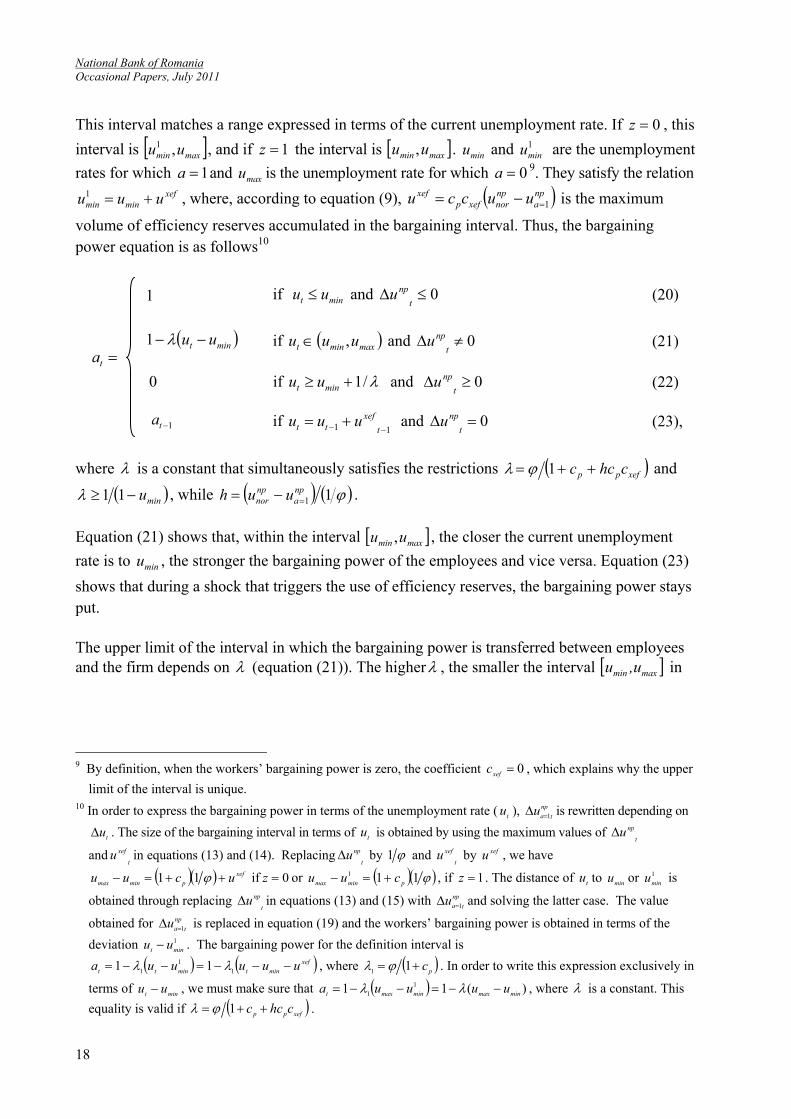
ta

This interval matches a range expressed in terms of the current unemployment rate. If 0z , this

interval is maxmin uu ,1 , and if 1z the interval is maxmin uu , . minu and 1minu are the unemployment

rates for which 1a and maxu is the unemployment rate for which 0a 9. They satisfy the relation xef

minmin uuu 1 , where, according to equation (9), npa

npnorxefp

xef uuccu 1 is the maximum

volume of efficiency reserves accumulated in the bargaining interval. Thus, the bargaining power equation is as follows10

1 if mint uu and 0t

npu (20),

mint uu 1 if maxmint uuu , and 0t

npu (21),

1ta if 11

t

xeftt uuu and 0

t

npu (23),

where is a constant that simultaneously satisfies the restrictions xefpp chcc 1 and

minu 11 , while 11npa

npnor uuh .

Equation (21) shows that, within the interval maxmin uu , , the closer the current unemployment

rate is to minu , the stronger the bargaining power of the employees and vice versa. Equation (23)

shows that during a shock that triggers the use of efficiency reserves, the bargaining power stays put.

The upper limit of the interval in which the bargaining power is transferred between employees and the firm depends on (equation (21)). The higher , the smaller the interval maxmin u,u in

9 By definition, when the workers’ bargaining power is zero, the coefficient 0xefc , which explains why the upper

limit of the interval is unique. 10 In order to express the bargaining power in terms of the unemployment rate ( tu ),

t

np

au 1 is rewritten depending on

tu . The size of the bargaining interval in terms of tu is obtained by using the maximum values of t

npu

andt

xefu in equations (13) and (14). Replacingt

npu by 1 and t

xefu by xefu , we have

xef

pminmax ucuu 11 if 0z or 111

pminmax cuu , if 1z . The distance of tu to minu or 1

minu is

obtained through replacing t

npu in equations (13) and (15) with t

npau 1 and solving the latter case. The value

obtained for t

npau 1 is replaced in equation (19) and the workers’ bargaining power is obtained in terms of the

deviation 1

mint uu . The bargaining power for the definition interval is

xef

mintmintt uuuuua 1

1

1 11 , where pc 11 . In order to write this expression exclusively in

terms of mint uu , we must make sure that )(11 1

1 minmaxminmaxt uuuua , where is a constant. This

equality is valid if xefpp chcc 1 .

0 if /1 mint uu and 0t

npu (22),


19

which the bargaining power influences the wage setting11. The employees and the firm have equal bargaining power when 2maxmint uuu .

The equation of the bargaining power is consistent with the idea that on a depressed labor market, the bargaining power of employees is small, because finding a job can prove difficult. This is reflected in the setting of a relatively low negotiated wage. Conversely, in a very strong labor market, the bargaining power of employees is high and the negotiated wage exceeds significantly the reservation wage.

2.2.2. The workers’ and employers’ surplus

Assuming that 0z , npnor

npat

np uuu ,1 and that the firm’s core business does not allow for

alternative uses of the capital, the remaining nominal unit labor surplus is 12

tstmintttttf WLufpLDpS 1 (24),

where tsW is the nominal wage received by the worker, f is a constant that represents the

weight of the fixed costs of production13 in the total production corresponding to the unemployment rate minu .

11 In turn, the lower , the higher pc and xefc . Thus, the larger the efficiency reserves, the wider the interval of the

unemployment rates for which a and mint uu are determined.

12 A similar definition is presented by Akerlof, Dickens and Perry (1996), in which tfS is defined in terms of *u .

To keep the equations simple, we decided to definetfS in relation to minu .

13 We could exclude f from the definition of the firm’s surplus, but we considered necessary to keep it, as in the

case of certain products like software, medicines, etc., the fixed costs hold a larger share in total costs than the marginal ones, so that the price reflects more the mark-up rather than the marginal costs.


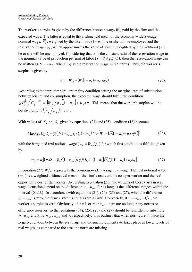
20

The worker’s surplus is given by the difference between wage tsW paid by the firm and the

expected wage. The latter is equal to the arithmetical mean of the economy-wide average nominal wage, tW , weighted by the likelihood ( tu1 ) he or she will be employed and the

reservation wage, tS , which approximates the value of leisure, weighted by the likelihood ( tu )

he or she will be unemployed. Considering that s is the constant ratio of the reservation wage to the nominal value of production per unit of labor ( LYpSs tt , then the reservation wage can

be written as tt psS , where s is the reservation wage in real terms. Thus, the worker’s

surplus is given by:

tttttste psuuWWS 1 (25).

According to the intra-temporal optimality condition setting the marginal rate of substitution between leisure and consumption, the expected wage should fulfill the condition

st

ut

ut

pt

Wt

Ct

L 1 . This means that the worker’s surplus will be

positive only if st

pt

W .

With values of fS and eS given by equations (24) and (25), condition (18) becomes

ta

ttttsta

ttmintttt psuuWWWLufpLDp 1 1Max t-1s (26),

with the bargained real notional wage ( ttsst pWw ) for which this condition is fulfilled given

by:

111 mins suupWaLpufpDpaw tttttttttttt (27).

In equation (27) pW represents the economy-wide average real wage. The real notional wage

( tsw ) is a weighted arithmetical mean of the firm’s real variable cost per worker and the real

opportunity cost of the worker. According to equation (21), the weights of these costs in real wage formation depend on the difference mint uu for as long as the difference ranges within the

interval /,10 . In accordance with equations (21), (24), (25) and (27), when the difference

mint uu is zero, the firm’s surplus equals zero as well. Conversely, if 1 mint uu , the

worker’s surplus is zero. Obviously, if 1z or nort uu , there are no longer any norms or

efficiency reserves, so that equations (24), (25), (26) and (27) should be rewritten to substitute , minu and by xef , 1

minu and 1 respectively. This outlines that when norms are in place the

negative relation between the real wage and the unemployment rate takes place at lower levels of

real wages, as compared to the case the norm are missing.


21

2.3. Equilibrium with flexible prices

For a representative firm, the labor market equilibrium is reached at the intersection point of supply and demand equations. The demand equation derives from the firm’s behavior in setting prices, while the supply equation is determined by the wage-setting mechanism. Both processes depend on real wages. Further in this section we will write the demand and supply equations and will introduce the concept of natural rate of unemployment.

2.3.1. Aggregate demand and supply equations on the labor market

Assuming further that 0z and npnor

npat

np uuu ,1 , a firm that produces final goods will set the

price p in order to maximize the difference

ββ /1/Max tttttttt ppCWppCp (28),

where 1tW is the nominal marginal cost of the firm. If prices are flexible, all the firms will

choose the same price, so that the difference in equation (28) is at its highest level for a constant value of the real wage tdtt wpW 14 equal to

μηββηw td 1 (29),

where 1 represents the best gross margin that a firm could add to the nominal

marginal cost.

Equation (29) represents the labor demand equation and it shows how the prices response to changes in wages. The equation describes the wage that is consistent with the willingness of the firm to hire, given the general conditions regarding commodity prices, the tax system, the interest rates, etc. Equation (29) is consistent with the fact that real wages are neutral to the business cycle. The constant value of the real wage results from both the constant elasticity of the demand equation (2) and the assumption that labor productivity is constant. An increase in labor productivity or demand elasticity relative to prices triggers the rise in tdw . From the

definition of nominal marginal cost it results that μηw td 1 is the real marginal cost of the

firm.

14 Equation (29) can be derived by making the distinction between the firms producing final goods, facing

monopolistic competition, and the firms producing intermediary goods, facing perfect competition. Profit maximization by the firms producing intermediary goods is conditional on the equality between real marginal labor income and real marginal cost: wPPI , where IP is the price of the intermediary good and P is the

price index associated with C . Profit maximization by the firms producing final goods requires that IPP .

By replacing the value of in the previous equation, we obtain equation (29).


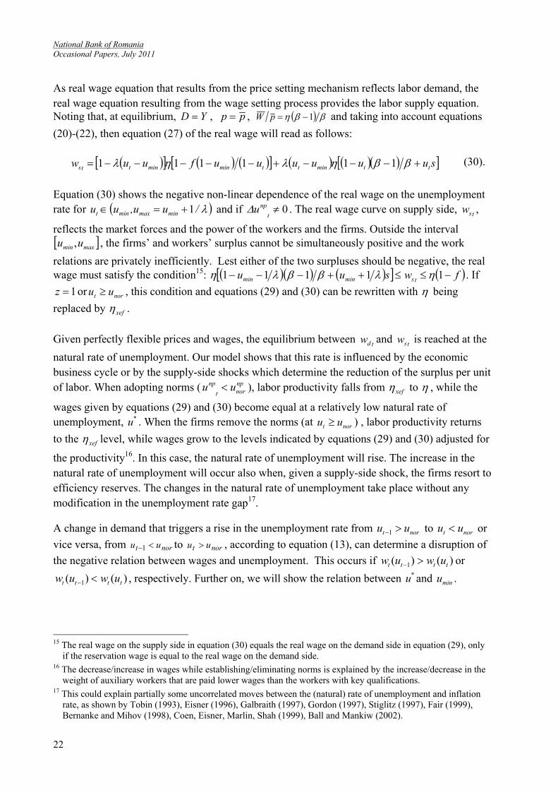
22

As real wage equation that results from the price setting mechanism reflects labor demand, the real wage equation resulting from the wage setting process provides the labor supply equation. Noting that, at equilibrium, YD , pp , 1 pW and taking into account equations

(20)-(22), then equation (27) of the real wage will read as follows:

suuuuuufuuw ttminttminmintts 111111 (30).

Equation (30) shows the negative non-linear dependence of the real wage on the unemployment rate for /uu,uu minmaxmint 1 and if 0

t

npu . The real wage curve on supply side, tsw ,

reflects the market forces and the power of the workers and the firms. Outside the interval maxmin uu , , the firms’ and workers’ surplus cannot be simultaneously positive and the work

relations are privately inefficiently. Lest either of the two surpluses should be negative, the real wage must satisfy the condition15: fwsuu tsminmin 11111 . If

1z or nort uu , this condition and equations (29) and (30) can be rewritten with being

replaced by xef .

Given perfectly flexible prices and wages, the equilibrium between tdw and tsw is reached at the

natural rate of unemployment. Our model shows that this rate is influenced by the economic business cycle or by the supply-side shocks which determine the reduction of the surplus per unit of labor. When adopting norms ( np

nort

np uu ), labor productivity falls from xef to , while the

wages given by equations (29) and (30) become equal at a relatively low natural rate of unemployment, *u . When the firms remove the norms (at nort uu ) , labor productivity returns

to the xef level, while wages grow to the levels indicated by equations (29) and (30) adjusted for

the productivity16. In this case, the natural rate of unemployment will rise. The increase in the natural rate of unemployment will occur also when, given a supply-side shock, the firms resort to efficiency reserves. The changes in the natural rate of unemployment take place without any modification in the unemployment rate gap17.

A change in demand that triggers a rise in the unemployment rate from nort uu 1 to nort uu or

vice versa, from nort uu 1 to nort uu , according to equation (13), can determine a disruption of

the negative relation between wages and unemployment. This occurs if )()( 1 tttt uwuw or

)()( 1 tttt uwuw , respectively. Further on, we will show the relation between *u and minu .

15 The real wage on the supply side in equation (30) equals the real wage on the demand side in equation (29), only

if the reservation wage is equal to the real wage on the demand side. 16 The decrease/increase in wages while establishing/eliminating norms is explained by the increase/decrease in the

weight of auxiliary workers that are paid lower wages than the workers with key qualifications. 17 This could explain partially some uncorrelated moves between the (natural) rate of unemployment and inflation

rate, as shown by Tobin (1993), Eisner (1996), Galbraith (1997), Gordon (1997), Stiglitz (1997), Fair (1999), Bernanke and Mihov (1998), Coen, Eisner, Marlin, Shah (1999), Ball and Mankiw (2002).


23

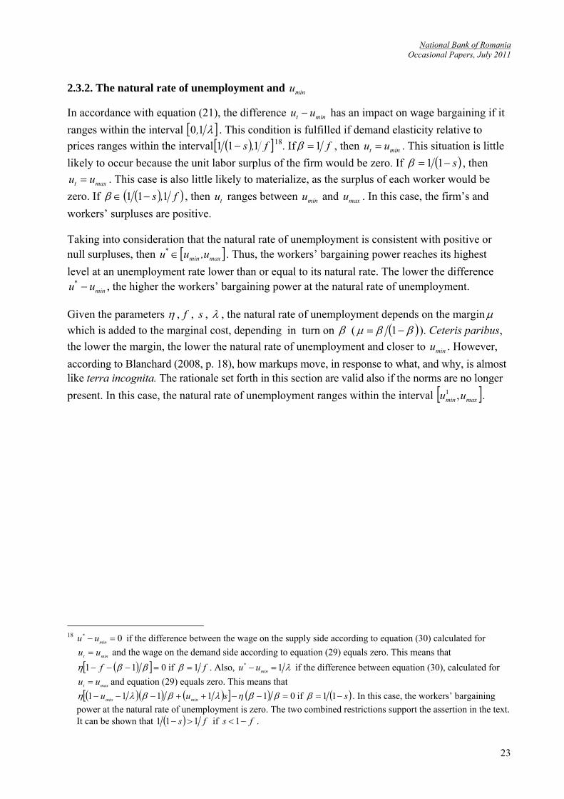
2.3.2. The natural rate of unemployment and minu

In accordance with equation (21), the difference mint uu has an impact on wage bargaining if it

ranges within the interval 10, . This condition is fulfilled if demand elasticity relative to

prices ranges within the interval f,s 111 18. If f1 , then mint uu . This situation is little

likely to occur because the unit labor surplus of the firm would be zero. If s 11 , then

maxt uu . This case is also little likely to materialize, as the surplus of each worker would be

zero. If f,s 111 , then tu ranges between minu and maxu . In this case, the firm’s and

workers’ surpluses are positive.

Taking into consideration that the natural rate of unemployment is consistent with positive or null surpluses, then maxmin

* u,uu . Thus, the workers’ bargaining power reaches its highest

level at an unemployment rate lower than or equal to its natural rate. The lower the difference

min* uu , the higher the workers’ bargaining power at the natural rate of unemployment.

Given the parameters , f , s , , the natural rate of unemployment depends on the margin

which is added to the marginal cost, depending in turn on ( 1 ). Ceteris paribus,

the lower the margin, the lower the natural rate of unemployment and closer to minu . However,

according to Blanchard (2008, p. 18), how markups move, in response to what, and why, is almost like terra incognita. The rationale set forth in this section are valid also if the norms are no longer

present. In this case, the natural rate of unemployment ranges within the interval maxmin uu ,1 .

18 0* minuu if the difference between the wage on the supply side according to equation (30) calculated for

mint uu and the wage on the demand side according to equation (29) equals zero. This means that

011 f if f1 . Also, 1* minuu if the difference between equation (30), calculated for

maxt uu and equation (29) equals zero. This means that

011111 suu minmin if s 11 . In this case, the workers’ bargaining

power at the natural rate of unemployment is zero. The two combined restrictions support the assertion in the text. It can be shown that fs 111 if fs 1 .


24

3. The power of bargaining and the temporary alternative wage setting mechanism

The presence of a surplus associated with the existing work relations means that any path of the real wage that allows for 0teS and 0

tfS for any t is compatible with the equilibrium

(Hall, 2005 and Blanchard and Gali, 2008). Nash negotiation generates one of these trajectories.

In this section we show that if the workers’ bargaining power is significantly higher than that of the firm, Nash negotiation can be temporarily replaced by an alternative wage setting mechanism (AWSM). This temporary mechanism leads to the simultaneous growth of real wage and unemployment rate. We first show under what conditions workers can use their bargaining power in order to increase the real wage above its notional level. Afterwards, we continue by analyzing what is the wage growth rate acceptable for a firm in order to preserve its surplus.

3.1. The bargaining power and the unemployment gap

One reason for which workers would want to use the bargaining power to increase real wage above its notional level could be the information asymmetry (Acemoglu, 1995). If workers have imperfect information regarding the total surplus associated with the employment relation, they could demand excessive increases of their wages. Another reason could be the inflation expectations following a loosening of monetary policy or fiscal policy stance to alter the proportion of surplus reallocation.

There are two conditions to be simultaneously satisfied in order for the workers to use their bargaining power for demanding a real wage above the notional value. The first condition is that the effective unemployment rate must be equal to or lower than the natural rate of unemployment ( *

t uu ). If this condition is not fulfilled, there is available labor force willing to work for a

wage equal to the notional level. If *t uu , then there is no more available labor force willing to

work for the notional wage. Thus, workers gain the power to demand wage increases above the notional level, being able to give up Nash negotiation.

The other condition is that the workers’ bargaining power must be higher than that of the firm ( 2maxmint uuu ) and the effective rate of unemployment must be sufficiently close to minu .

This condition is fulfilled if, given the parameters minu , f , s and (the latter depending on ,

pc and xefc ), the markup is sufficiently low, reflecting the firms’ small market power.

Formalizing, this condition would mean that xt uu , where 2maxminminx uu,uu is the

maximum value of tu at which workers can impose wages above the notional level.

The previous condition means also that *u must be close enough to minu . The two unemployment rates are sufficiently close if the markup is sufficiently low, reflecting the firms’ small market

power. If 2maxmin* uuu , *u could be higher than, lower than or equal to xu . By combining


25

the two conditions, it results that the workers’ bargaining power can be used for wage increases above the notional level if xt uu and x

* uu or if *t uu and x

* uu .

The case where x*

t uuu shows clearly that the real wage could rise above the notional level

due to the workers’ high bargaining power, although there is no excess demand. Obviously, in the case of an inflationary gap of unemployment rate ( x

*t uuu or *uuu xt ), the

probability of the high bargaining power to be used for increasing real wages above the notional level is even higher.

The cases described above are essential as far as this paper is concerned. They allow us to show the microeconomic rationale of shifting to AWSM, which leads to the simultaneous increase of the real wage and unemployment rate. Further on, we show this rationale.

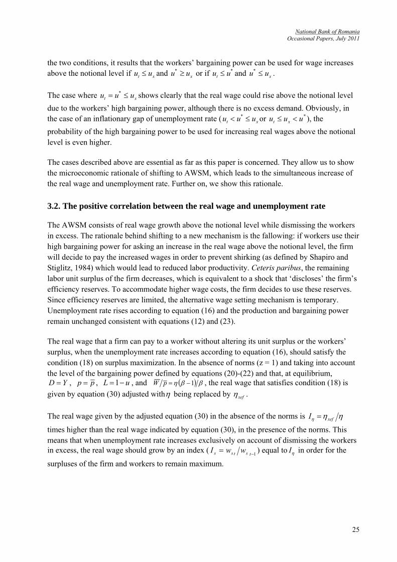
3.2. The positive correlation between the real wage and unemployment rate

The AWSM consists of real wage growth above the notional level while dismissing the workers in excess. The rationale behind shifting to a new mechanism is the fallowing: if workers use their high bargaining power for asking an increase in the real wage above the notional level, the firm will decide to pay the increased wages in order to prevent shirking (as defined by Shapiro and Stiglitz, 1984) which would lead to reduced labor productivity. Ceteris paribus, the remaining labor unit surplus of the firm decreases, which is equivalent to a shock that ‘discloses’ the firm’s efficiency reserves. To accommodate higher wage costs, the firm decides to use these reserves. Since efficiency reserves are limited, the alternative wage setting mechanism is temporary. Unemployment rate rises according to equation (16) and the production and bargaining power remain unchanged consistent with equations (12) and (23).

The real wage that a firm can pay to a worker without altering its unit surplus or the workers’ surplus, when the unemployment rate increases according to equation (16), should satisfy the condition (18) on surplus maximization. In the absence of norms (z = 1) and taking into account the level of the bargaining power defined by equations (20)-(22) and that, at equilibrium,

YD , pp , uL 1 , and 1 pW , the real wage that satisfies condition (18) is

given by equation (30) adjusted with being replaced by xef .

The real wage given by the adjusted equation (30) in the absence of the norms is xefI

times higher than the real wage indicated by equation (30), in the presence of the norms. This means that when unemployment rate increases exclusively on account of dismissing the workers in excess, the real wage should grow by an index (

1

tstss wwI ) equal to I in order for the

surpluses of the firm and workers to remain maximum.


26


27


28

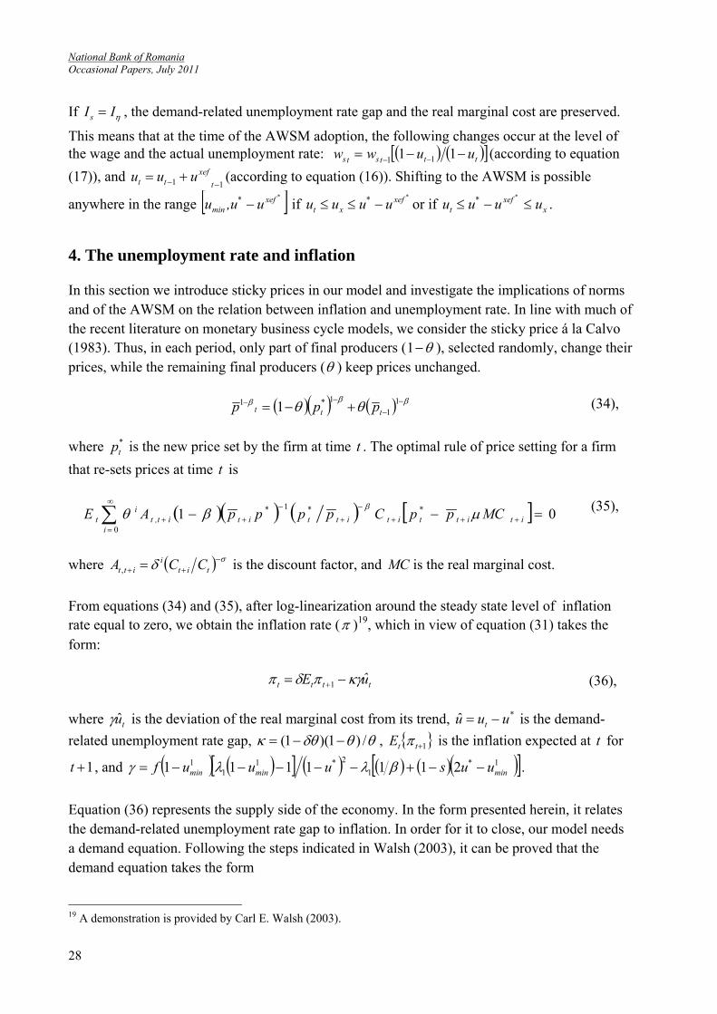
If IIs , the demand-related unemployment rate gap and the real marginal cost are preserved.

This means that at the time of the AWSM adoption, the following changes occur at the level of the wage and the actual unemployment rate: tttsts uuww 11 11 (according to equation

(17)), and 11

t

xeftt uuu (according to equation (16)). Shifting to the AWSM is possible

anywhere in the range *xef*min uu,u if

*xef*xt uuuu or if x

xef*t uuuu

*

.

4. The unemployment rate and inflation

In this section we introduce sticky prices in our model and investigate the implications of norms and of the AWSM on the relation between inflation and unemployment rate. In line with much of the recent literature on monetary business cycle models, we consider the sticky price á la Calvo (1983). Thus, in each period, only part of final producers ( 1 ), selected randomly, change their prices, while the remaining final producers ( ) keep prices unchanged.

11

1*1 1 ttt ppp (34),

where *tp is the new price set by the firm at time t . The optimal rule of price setting for a firm

that re-sets prices at time t is

011

0

itit

*titit

*t

*it

iit,t

it MCppCppppAE

(35),

where tit

iitt CCA , is the discount factor, and MC is the real marginal cost.

From equations (34) and (35), after log-linearization around the steady state level of inflation rate equal to zero, we obtain the inflation rate ( )19, which in view of equation (31) takes the form:

tttt uE 1 (36),

where tu is the deviation of the real marginal cost from its trend, *ˆ uuu t is the demand-

related unemployment rate gap, /)1)(1( , 1ttE is the inflation expected at t for

1t , and 11

211

1 2111111 min**

minmin uusuuuf .

Equation (36) represents the supply side of the economy. In the form presented herein, it relates the demand-related unemployment rate gap to inflation. In order for it to close, our model needs a demand equation. Following the steps indicated in Walsh (2003), it can be proved that the demand equation takes the form

19 A demonstration is provided by Carl E. Walsh (2003).


29

adjustment of inflation is relatively large and has an opposite sign if employment is relatively high when maxnort uuu . The response of the unemployment rate is lower for low levels of

employment, when nort uu (equation (15)). Depending on the size of the response, adjustments

in unemployment gap in equation (34) are larger or lower respectively. This can be an explanation for the counterintuitive fact that, sometimes (Fair, 1999), for relatively high levels of employment the Philips curve is relatively flatter.

To show the implications of AWSM on the correlation between inflation rate and unemployment, rate we assume the economy is functioning at the natural rate of unemployment. Adopting AWSM means that the effective rate of unemployment and the natural rate of unemployment grow at the same time by the same amount as described in equation (16). Equation (34) allows us to show that the evolution of the inflation rate depends on the causes behind AWSM adoption.

If the cause is represented by the information asymmetry, inflation rate will remain unchanged. However, an easing of the monetary policy stance in order to bring the unemployment rate back to the level prior to AWSM adoption generates a negative gap which in turn determines the increase in inflation. As it is unsustainable at the new level, the unemployment rate returns to its natural level in the medium term. Finally, the economy is functioning at relatively high wages, inflation and unemployment rates. The wage and the unemployment rate remain relatively high until the conditions for adopting the norms are satisfied again.

However, if the cause is the anticipation of an easing of the monetary policy stance, inflation expectations emerge and the inflation rate increases due to the component 1ttE in equation

(34). Thus, the anticipation of an easing of the monetary policy stance which leads to AWSM adoption triggers the simultaneous growth of unemployment and inflation. The real interest rate falls, causing aggregate demand to increase and unemployment rate to decrease.

If the easing of the monetary policy stance offsets completely the growth of the unemployment rate implied by AWSM, then the combined effect is a higher inflation. This result is in line with the results presented in the papers by Kidland and Prescott (1977), Baro and Gordon (1983) and others. If the easing of the monetary policy stance is not completely reversing the increase in the unemployment rate implied by AWSM, then both inflation and unemployment will grow. In other words, a looser monetary policy stance may result in the simultaneous growth of the inflation rate and the unemployment rate if AWSM is adopted following the expectations of an easing of the monetary policy stance.

It is reasonable to assume that the firms that change prices ( 1 ) choose to pass the wage growth on prices. In this case, the use of efficiency reserves is a gradual process. In a first stage, only the firms that do not change prices ( ) will adopt AWSM. Thus, inflation and unemployment will rise simultaneously. In the following stages, the firms that did not use the


30

efficiency reserves will want to use them insofar as their competitors that had already done that are going to increase prices. This pushes unemployment rate higher. However, because the firms that change prices are selected at random, it remains uncertain if inflation and unemployment increase simultaneously in the following adjustment stages.

5. Conclusions

The model presented in this paper shows that if the firms set norms that entail hiring auxiliary workers in excess and the workers’ bargaining power depends on the unemployment rate, then the negative relation between inflation and the unemployment rate can be temporarily interrupted. In the presence of norms, labor productivity, the unemployment rate and the real wage are relatively low. Besides the natural rate of unemployment, there are also other levels of the unemployment rate that are relevant to monetary policy decisions.

The unemployment rate noru below which the norms are set is relevant to the changes in labor

productivity and to the effects of a shift in the monetary policy stance on the unemployment rate. When the unemployment rate falls below noru , firms establish norms that entail excess workers,

which causes a shock that reduces the unemployment rate irrespective of the changes in aggregate demand. Thus, there is a negative shock on labor productivity. Conversely, when the unemployment rate becomes equal to (or higher than) noru , the firms remove the norms no longer

entailing workers in excess, while the unemployment rate becomes exclusively reliant on the changes in aggregate demand. Thus, there is a positive shock on labor productivity. Monetary policy aiming to achieve a certain inflation adjustment causes higher changes in the unemployment rate in the presence of the norms ( nort uu ) as compared to the opposite situation.

The unemployment rate at which the bargaining power of workers is maximum, minu , may be

relevant to the relation between inflation and unemployment and to the monetary policy. Thus, it is relevant when the effective rate of unemployment is equal to (or lower than) the natural rate of unemployment and sufficiently close to minu . Ceteris paribus, the lower the natural rate of

unemployment, and thus closer to minu , the lower the markup that monopolistic firms add to the

marginal cost.

When these conditions are fulfilled, the workers, using their high bargaining power, can force the firm to shift from Nash negotiation of wages to a temporary alternative wage setting mechanism (AWSM). This mechanism consist in wage increases above the notional level (the workers have the power to impose this), while removing the norms and dismissing the workers in excess. AWSM preserves the proportion to which the surplus associated with work relation is shared between the firm and the workers and leads to a temporary interruption of the negative relation between the inflation rate and the unemployment rate. Compared to the situation seen before the firms’ using the efficiency reserves, the wage, the inflation rate, unemployment rate and labor productivity are relatively high until the condition for adopting the norms is satisfied again.


31

The reason behind the AWSM adoption is relevant to the relation between inflation and unemployment. In order to show this, we assume the economy is functioning at the natural rate of unemployment. If the adoption of AWSM is caused by the fact that workers have imperfect information regarding the level of the surplus associated with work relations, the unemployment rate will increase without any change in inflation or the unemployment rate gap. However, if AWSM adoption is determined by the workers’ expectation of the monetary policy stance loosening, inflation and unemployment will increase simultaneously, while the unemployment gap will remain unchanged.

After dismissing the workers in excess, the relation between inflation and unemployment turns negative again. In the short term, an easing of the monetary policy stance focusing on lowering the unemployment rate to the level seen before resorting to the efficiency reserves increases the unemployment gap and, thus, the inflation rate. As the unemployment rate is unsustainable at this level, it returns in the medium term to its natural level.

The monetary policy should not seek to counterbalance the increase in unemployment implied by giving up norms due to the fall in demand or to AWSM adoption. However, in practice, it is difficult to identify those changes in the unemployment rate and the labor productivity that reflect the above mentioned causes.

The norms and the AWSM can explain in part why the relation between inflation and the unemployment rate is mysterious, as defined by Mankiw (2000). They support the idea that the relation between inflation and unemployment is influenced by the interaction between monetary policy and the labor market. On the one hand, the labor market influences the monetary policy effects on the relation between inflation rate and unemployment rate. In our model this fact is due to norms. On the other hand, the expectations regarding the changes to the monetary policy stance influence the labor market. In our model, this aspect determines the adoption of AWSM, which leads to the simultaneous growth of inflation and unemployment.


32

References

Acemoglu, Daron Asymmetric Information Bargaining and Unemployment Fluctuations,

International Economic Review, 1995 Akerlof, A. George The Missing Motivation in Macroeconomics, American Economic

Association, Chicago, (January 6), 2007 Akerlof, A. George, Dickens, T. William, Perry, L. George

The Macroeconomics of Low Inflation, Brooking Papers on Economic Activity, Vol. 1996, No. 1, p. 1-76, 1996

Ball, Laurence, Mankiw, N. Gregory

The NAIRU in Theory and Practice, The Journal of Economic Perspectives, Vol. 16, No. 4 (Autumn), p. 115-136, 2002

Baro, J. Robert, Gordon, David

Rules, Discretion and Reputation, in a Model of Monetary Policy, Journal of Monetary Economics, Vol. 12, No. 1 (July), p. 101-121, 1983

Bernanke, Ben, Mihov, Ilian

The Liquidity Effect and Long-Run Neutrality, NBER, Working Paper 6608 (June), 1998

Blanchflower, David, Oswald, Andrew

The Wage Curve, Cambridge, Mass. and London: Massachusetts Institute of Technology Press (Quote by Blanchard and Katz, 1997), 1994

Blanchard, Olivier, Katz, F. Laurence

What We Know and Do Not Know About the Natural Rate of Unemployment, The Journal of Economic Perspectives, Vol. 11, No. 1 (Winter), p. 51-72, 1997

Blanchard, Olivier Is There a Core of Usable Macroeconomics?, The American

Economic Review, Vol. 87, No. 2, Papers and Proceedings of the Hundred and Fourth Annual Meeting of the American Economic Association (May), p. 244-246, 1997

Blanchard, Olivier, Gali, Jordi

Labour Markets and Monetary Policy: A New Keynesian Model with Unemployment, Working Paper 13897, National Bureau of Economic Research, Cambridge (March), 2008

Blanchard, Olivier The State of Macro, Working Paper 14259, National Bureau of

Economic Research, Cambridge (August), 2008 Calvo, A. Guillermo Staggered Prices in a Utility-Maximizing Framework, Journal of

Monetary Economics, Vol. 12(3), (September), p. 383-398, 1983 Coen, M. Robert, Eisner, Robert, Marlin, J. Tepper, Shah, N. Suken

The NAIRU and Wages in Local Labour Markets, The American Economic Review, Vol. 89, No. 2, Papers and Proceedings of the One Hundred Eleventh Annual Meeting of the American Economic Association (May), p. 52-57, 1999


33

Eisner, Robert A New View of the NAIRU, mimeo, Northwestern University, June 4,

1996 presented to the 7th World Economic Congress, Tokyo, August 1995; in Davidson, P., and Kregel, J., eds., “Improving the Global Economy: Keynesianism and the Growth of Output and Employment”. Cheltingham, UK, and Brookfield: Eduard Elgar, October 1997 (Quote by Galbraith, 1997)

Fair, C. Ray Does the NAIRU Have the Right Dynamics?, The American Economic

Review, Vol. 89, No. 2, Papers and Proceedings of the One Hundred Eleventh Annual Meeting of the American Economic Association (May), p. 58-62, 1999

Friedman, Milton The Role of Monetary Policy, The American Economic Review, Vol. 58,

No. 1 (March), p. 1-17, 1968 Galbraith, K. James Time to Ditch the NAIRU, The Journal of Economic Perspectives,

Vol. 11, No. 1 (Winter), p. 93-108, 1997 Gordon, J. Robert The Time-Varying NAIRU and its Implications for Economic Policy,

The Journal of Economic Perspectives, Vol. 11, No. 1 (Winter), p. 11-32, 1997

Hall, E. Robert Employment Fluctuations with Equilibrium Wage Stickiness, American

Economic Review, Vol. 95, No. 1, p. 50-64, 2005 Kydland, E. Finn, Prescott, C. Edward

Rules Rather than Discretion: The Inconsistency of Optimal Plans, Journal of Political Economy, Vol. 85. No. 3 (June), p. 473-92, 1977

Mankiw, N. Gregory The Inexorable and Mysterious Trade-off between Inflation and

Unemployment, NBER Working Paper 788, 2000 Phelps, S. Edmund Money-Wage Dynamics and Labour-Market Equilibrium, The Journal

of Political Economy, Vol. 76, No. 4, Part 2: Issues in Monetary Research, 1967 (July-August), p. 678-711, 1968

Shapiro, Carl, Stiglitz, Joseph

Equilibrium Unemployment as a Discipline Device, în American Economic Review, Vol. 74, (June), p. 433-44, 1984

Stiglitz, Joseph Reflections on the Natural Rate Hypothesis, The Journal of Economic

Perspectives, Vol. 11, No. 1 (Winter), p. 3-10, 1997 Tobin, James Price Flexibility and Output Stability: An Old Keynesian View,

The Journal of Economic Perspectives, Vol. 7, No. 1 (Winter), p. 45-65, 1993

Vickers, John Concepts of Competition, Oxford University Press, Vol. 47 (1), (January)

p. 1-23,1995 Walsh, E. Carl Monetary Theory and Policy, MIT Press, p. 230-237, 2003

occasional papers no.8 iul11 - bnro.ro · the presence of norms, in certain conditions, the...

Documents