occasional paper series - european central bank · occasional paper series . business investment in...

Occasional Paper Series Business investment in EU countries

WGEM Team on Investment

No 215 / October 2018

Disclaimer: This paper should not be reported as representing the views of the European Central Bank (ECB). The views expressed are those of the authors and do not necessarily reflect those of the ECB.

Working Group on Econometric Modelling

ECB Occasional Paper Series No 215 / October 2018

1

Contents

Abstract 2

Executive summary 3

1 Introduction 6

2 Is investment low? 8

3 Drivers of investment 13

3.1 Evidence from VARs with recursive identification 13

3.2 What role does uncertainty play for investment? 18

3.3 Importance of credit supply shocks – results from VARs with sign restrictions 24

3.4 Other (secular) developments in investment 36

4 The role of public investment 43

4.1 Motivation 43

4.2 Small open economies 45

4.3 Single-country and broad-based expansions 51

4.4 Discussion 57

5 Capital misallocation: some stylised facts and determinants 60

5.1 Measurement of within-sector capital misallocation 60

5.2 Developments in capital misallocation 62

5.3 Determinants of capital misallocation 66

5.4 Policy implications 71

6 Summary and conclusions 72

References 76

Methodological annex 91

A Accelerator model 91

B Bayesian VAR model with recursive (Cholesky) identification 92

C Measurement of input misallocation 94

D Determinants of input misallocation 98


2

Abstract

The article analyses recent developments in business investment for a large group of EU countries, using a broad set of analytical tools and data sources. We find that the assessment of whether or not investment is currently low varies across benchmarks and countries. At the euro area level and for most countries, the level of business investment is broadly in line with the level of overall activity. However rates of capital stock growth have slowed down since the crisis. The main cyclical determinants of investment developments in the euro area include foreign and domestic demand, uncertainty and financial conditions. Uncertainty seems to have played a negative role during the financial and sovereign debt crises; however, given its low levels more recently, it has not acted as a drag on business investment overall during the recovery. Credit constraints appear to have hindered investment during the twin crises, especially in stressed countries. Aside from cyclical developments, important secular factors – relating to demographics, the changing nature and location of production, and the business environment – have influenced investment. Another factor that may have amplified the decline in private investment, particularly in countries that were hit hardest by the sovereign debt crisis, is the low level of public investment. This is because when public investment enhances the productivity of the private sector, there may be positive spillovers from the former to the latter, including across countries. Finally, intra-sector capital misallocation, measured as the within-sector dispersion across firms in the marginal revenue product of capital, has been increasing in Europe since 2002, which may in turn have exerted a significant drag on total factor productivity dynamics, and hence on aggregate output growth.

Keywords: business investment, uncertainty, monetary policy, capital misallocation.

JEL codes: E32, E52, E62, D24, D61.


3

Executive summary

Many analysts and international institutions have judged the performance of investment since the global financial crisis to be disappointing. To prepare well-grounded macroeconomic projections and (monetary) policy proposals, it is important: to understand whether investment has indeed been weak and what the drivers behind this have been; to assess the effectiveness of different monetary policy measures and how these may interact with other (e.g. fiscal) policies; and to identify different sources of uncertainty in the context of a continuously evolving economic environment. This paper aims to provide a wide range of perspectives on investment, using a broad set of analytical tools and data sources, for a large group of EU countries, focusing on the most recent developments and policy-relevant research questions.

The various sections of the paper address the following four questions: First, has investment been low since the financial crisis? Second, what factors can (help) explain investment developments? Third, what is the role of public investment, and how does it interact with monetary policy? Fourth, has capital been allocated efficiently across firms in Europe, and what policies may contribute to reducing capital misallocation?

The focus of the analysis is on private non-residential (“business”) investment, as one of the key drivers of the productive capacity of the economy.

The main findings of the study are as follows:

The assessment of whether investment is low or not varies across benchmarks and countries. Business investment in the euro area has only recently approached pre-crisis levels, and in some countries it remains well below those levels. For the euro area as a whole, and for most individual countries, the level of business investment is broadly in line with the level of overall activity, according to the historical relationship between these two variables. There are, however, some countries with substantial persistent gaps (according to this metric). Even though for many countries investment has performed in line with other expenditure components, rates of capital stock growth show declining dynamism following the crisis, raising the prospect of persistently low growth in the future. These developments may to some extent reflect expected trends in demographics and the excess installed capacity still to be fully absorbed in some countries and sectors. An important consideration relates to under-measurement of investment, as intangible assets are only partially covered in official statistics.

The main cyclical determinants of investment developments in the euro area include foreign and domestic demand, uncertainty and financial conditions. In the light of the slowdown in global trade following the financial crisis, euro area foreign demand appears to have led to less dynamic business investment during 2013-16. Uncertainty seems to have played a negative role during the financial and sovereign debt crises; however, given its low levels more recently, it has not acted as a drag on business investment overall during the recovery. Credit constraints, including in


4

relation to firms’ financial health, appear to have hindered investment during the twin crises, especially in stressed countries. The negative impact of those constraints appears to have largely subsided more recently, and low real interest rates have been also supportive, suggesting that the extensive set of monetary policy measures has helped investment activity. There is some heterogeneity across countries and firms as to the relative importance of the various drivers, highlighting the value of more granular analysis. Importantly, there are sizeable uncertainties in quantifying the contribution of different factors, including but not limited to measurement and identification. A rich modelling toolbox and broad set of perspectives are therefore useful when assessing investment developments.

Aside from cyclical developments and demographics, other important secular factors – relating to the changing nature and location of production and to the business environment – have influenced investment. The productive structure of the economy has been shifting towards the services sector and advanced technological applications, accompanied by a marked increase in expenditure on intellectual property products. This brings with it potential changes in financing needs, higher capital replacement requirements and, more generally, changes in the relationship between investment and its determinants. The effects of the gradual globalisation of production and of the increasing importance of foreign direct investment on domestic investment are not necessarily adverse. Finally, the importance of the business environment and of the regulatory and institutional framework in stimulating investment has been highlighted by numerous studies, underlying the need for continued reform implementation efforts.

Another factor that may have amplified the decline in private investment, particularly in countries that were hit hardest by the sovereign debt crisis, is the low level of public investment. If public investment enhances the productivity of the private sector, there are positive spillovers from the former to the latter, although the magnitude of the effect depends on how public investment is financed. Budget-neutral financing by redirection of public spending from consumption to investment appears most appropriate, especially at times of limited fiscal space. An expansion in public investment in a large country can have positive effects on private investment in small economies that are its trading partners, if monetary policy is accommodative. The effect of public investment expansions can be significantly enhanced by broader-based actions if several countries increase their expenditure. In this case, the usual crowding-out effects on private investment stemming from the implementation of a standard monetary policy rule are attenuated (if the expanding country is large enough). Expansionary effects are stronger if the monetary authority credibly implements forward guidance (committing to keeping rates unchanged for a period, irrespective of the macroeconomic developments) or implements quantitative easing. However, the impact on GDP and other demand components is reduced if public investment is not productive or if there are significant delays in its execution.

Aside from the volume of capital stock, total factor productivity is a key determinant of economic growth. This in turn is affected by how efficiently capital is allocated across firms. Intra-sector capital misallocation, measured as the within-sector dispersion across firms in their marginal revenue product of capital, has


5

been increasing in Europe since 2002, with only temporary reductions recorded in some countries in the early years of the crisis. An analysis of the potential determinants of capital misallocation (demand, demand uncertainty, credit constraints and regulation) points to a significant role for policy in enhancing the efficient allocation of capital, via reforms in product and financial markets. It also highlights the (unresolved) ongoing debate over the role of the cost and supply of credit in driving allocative inefficiency.


6

1 Introduction

Many analysts and international institutions have identified the performance of investment since the global financial crisis as disappointing; see, for example, Banerjee et al. (2015), ECB (2017), EIB (2017), European Commission (2017), IMF (2015), OECD (2015) and World Bank (2017).1 Against the background of perceived general weakness in investment, marked heterogeneity across countries, assets and sectors has also been observed. These studies focus on different country compositions and use different subcomponents of investment (e.g. total, private, public or private non-residential investment) and a different selection of metrics or benchmarks to assess investment activity. While there is consensus on the most likely determinants of investment developments – typically (expected) demand, uncertainty and financing conditions/constraints – their relative importance often varies across studies. In addition, some important questions often remain unaddressed, such as the relationship between public and private investment and the issue of efficient allocation of capital across companies.

To prepare well-grounded macroeconomic projections and (monetary) policy proposals, it is important: to understand whether investment has indeed been weak and what the drivers behind this have been; to assess the effectiveness of different monetary policy measures and how they may interact with other (e.g. fiscal) policies; and to identify different sources of uncertainty within a continuously evolving economic environment.

This paper aims to provide a wide range of perspectives on investment for a large group of EU countries, focusing on the most recent developments and policy research questions. In particular, we consider:

• a wide range of benchmarks for assessing investment activity;

• different analytical tools, comprising time series and structural (DSGE) models and different identification strategies;

• both macro and micro (firm-level) evidence;

• both cyclical and secular drivers of investment;

• spillovers from public to private investment in a number of scenarios;

• the level of capital stock and its allocation across firms, with the latter being an important driver of total factor productivity.

Given the scope of the analysis, different dimensions of policies are discussed, including monetary, fiscal and structural aspects. We also review the recent literature

1 Other related studies of investment developments in the euro area (countries) include Balta (2015),

Banco de España (2016), Barkbu et al. (2015), Butzen et al. (2016), Deutsche Bundesbank (2016), Lewis et al. (2014) and Vermeulen (2016).


7

and relate our results to this. Including both aggregate euro area and individual-country perspectives is important, as the former can mask diverse trends and country-specific drivers. Quantitative analysis mainly focuses on the medium-term (cyclical) drivers; the discussion of long-term drivers is more descriptive and refers to other studies.

The individual sections of the paper aim to address the following questions.

• Has investment been low since the global financial crisis? (Section 2)

• What factors can (help) explain investment developments? (Section 3)

• What is the role of public investment, and how does it interact with monetary policy? (Section 4)

• Is capital allocated efficiently across firms in Europe, and what policies can contribute to reducing capital misallocation? (Section 5)

Section 6 provides a summary and conclusions. The Annex contains some details of the modelling approaches adopted.

The focus of the analysis is on private non-residential (“business”) investment as one of the key drivers of the productive capacity of the economy. Compared with business investment, residential and public investment often exhibit different behaviour over the business cycle, can be driven by different determinants and can be affected by different types of policies. There is also more controversy over the “productivity” of these types of investment. We discuss the role of public investment to the extent that it can affect private investment; a detailed analysis of developments in residential2 and public investment is beyond the scope of this paper.

It should be stressed that, in contrast to the United States, for example, there are no official data on business investment for most EU countries. The analysis is based on the estimates of the private non-residential part of investment derived by the national central banks (NCBs) of the European System of Central Banks (ESCB).3 The data vintage is May 2017, and the last data point is taken to be Q4 2016.4 In addition to the aggregate euro area, the following EU countries are comprised in the analysis: Denmark, Germany, Ireland, Greece, Spain, France, Croatia, Italy, Cyprus, Latvia, Netherlands, Portugal, Slovakia, Finland.

Some comparisons with the United States are also undertaken. 2 Regarding residential investment, see, for example, De Bandt et al. (2010) for a comprehensive study

and Andrews et al. (2011) for an assessment of policies. 3 Given the limited data availability for most of the countries, the business investment series used in this

paper is obtained as a residual, i.e. by subtracting public and residential investment from the total. The data for the euro area as a whole are derived via aggregation of country data; at the outset the sample was constructed based on a subset of available country data. For Cyprus and Ireland, the data have been further modified to account for special factors and outliers (most notably related to the activities of special-purpose entities in the case of Cyprus, and of large multinationals in the case of Ireland). For Spain, non-construction investment is used (i.e. the series contains machinery and equipment and weapons systems, intellectual property products and cultivated biological resources, for which the public-related investment content is estimated at between 10% and 15%). For Croatia, only data on total investment are available.

4 Note that some data revisions may have occurred since May 2017. In Germany, for instance, investment activity was significantly revised upwards, in particular for 2015 and 2016.


8

2 Is investment low?

The assessment of whether investment is high or low depends on the chosen benchmark. A number of different benchmarks have been considered in various studies, including past average growth rates, pre-crisis levels, past recoveries, developments in other expenditure components, investment-to-output ratios and (conditional) fit of time series models. This section considers some of these benchmarks for the euro area as a whole and for the individual countries, and also discusses their caveats.

One commonly used approach when assessing current investment expenditure is the comparison with pre-crisis levels. Chart 1 compares the business investment (and GDP) levels in 2016 with those in 2007 for the euro area and the countries under study.5 Even if more resilient than residential or public investment, business investment in the euro area only approached its 2007 levels in 2016, eight years after the onset of the financial crisis. By comparison, the level of business investment in the United States in 2016 was more than 10% higher than in 2007. However, the United States did not suffer a double dip recession and is currently at a more “mature” stage in the business cycle. A second observation is that the picture is very heterogeneous across countries. In some countries, business investment is still well below its 2007 level, particularly in some of the (previously) stressed countries. In a few others, it has surpassed its pre-crisis level. An important caveat of such a comparison is that the pre-crisis level might not be an appropriate benchmark, as there may have been some over-investment in some countries and sectors prior to the crisis (most notably in the construction sector).6

In general, a low level of investment may simply reflect the weakness in overall economic activity, as a result of the financial and sovereign debt crises.7 Compared with pre-crisis levels, GDP has recovered faster than investment in most countries (see Chart 1). However, this appears to be a typical pattern of the business cycle. Specifically, the investment-to-GDP ratio tends to be procyclical: investment falls more strongly during recessions than overall activity and recovers (relative to activity) when the cycle becomes more mature. At the end of 2016, the investment-to-GDP ratio (in real terms) in the euro area was above its historical average (it exceeded the average

5 In the cross-country comparisons, euro area countries are ordered according to their euro area GDP in

2016, followed by the non-euro area EU countries and the United States. 6 Another popular benchmark is the comparison of the developments in the level of investment in the

current and previous recoveries (e.g. Vermeulen, 2016). For business investment in the euro area, the conclusion is sensitive to the choice of normalisation (at the peak versus at the trough of the cycle) and whether or not the financial and sovereign debt crises are treated as a single episode.

7 For example, Vermeulen (2016) argues that the recovery in investment has been stronger than the recovery in consumption.


9

at the beginning of 2015), but still below the values recorded in previous upswings in the economic cycle.8

Chart 1 Real business investment and GDP in 2016

(percentage relative to 2007)

Sources: US Bureau of Economic Analysis, ECB and NCBs of the ESCB, NSIs and own calculations. Notes: Non-construction investment is reported for Spain; total investment is reported for Croatia. For Ireland, the comparison uses 2014 (instead of 2016), as in the following years investment and GDP levels were strongly affected by the activity of a few multinational enterprises. Data for Cyprus have been cleaned of some special factors.

We use a standard accelerator model to better assess whether the recovery in business investment has been in line with that of aggregate economic activity, according to the historical relationship between these two variables. The model relates the level of investment to distributed lags of changes in GDP (both rescaled by potential output).9 Chart 2 compares the fit of the model (conditional on GDP) with actual investment in 2016 for the euro area and the countries under study. Actual investment in the euro area was somewhat below the model fit in 2016, although the difference is within the historical variation. For many countries the differences are not significant. For others, however, the gaps are sizeable (significantly so in the cases of Italy, Portugal and Latvia).10

8 The picture is somewhat less “positive” when looking at the investment-to-GDP ratio in nominal terms,

due to the decline in the relative prices of investment goods. We focus on variables in real terms throughout the analysis. However, it should be kept in mind that using real ratios based on chained linked values is problematic due to lack of additivity (the sum of ratios does not equal one and the ratio cannot be interpreted as a share, see Whelan, 2000). Close to the base year, the problem is small, but it could be sizeable further back in the past.

9 We largely follow the implementation of Clark (1979) but estimated in a Bayesian framework, see the Annex for details.

10 For some countries, the uncertainty around the fit is very large. This often relates to the short estimation sample or the volatility of the series. For some countries the results are also sensitive to the estimation sample. When taking averages over the 2015-16 period, the results are qualitatively similar to those for 2016 only.

-50%

-40%

-30%

-20%

-10%

0%

10%

20%

30%

Euroarea

DE FR IT ES* NL IE* FI GR PT SK LV CY* DK HR* US

Business investmentGDP


10

Chart 2 Real business investment and accelerator model fit in 2016

(percentage deviation of outcome from model fit)

Sources: BEA, CBO, ECB and NCBs of the ESCB, NSIs and own calculations. Notes: Negative (positive) values mean that investment is x% lower (higher) than the model fit. ‘High’ and ‘Low’ values are based on 95% and 5% quantiles of the distribution of the model fit. Non-construction investment is used for Spain; total investment is used for Croatia. Data for Ireland and Cyprus have been cleaned of some special factors.

Several studies have included further variables in the accelerator (or similar) model to shed light on other possible drivers of investment during the crisis (see, for example, Banerjee et al., 2015; Barkbu et al., 2015; Bussière et al., 2015; Butzen et al., 2015; Fay et al., 2017; OECD, 2015). Such extensions typically include measures of financing conditions, uncertainty, foreign demand or the regulatory environment. We look in more detail at the role of various drivers via the lens of vector autoregression (VAR) models in the next section.

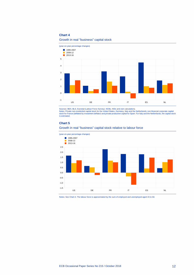
While the evidence above shows that, overall, business investment has been in line with the level of economic activity in the euro area and many of the individual countries, it does not address two important concerns. First, the analysis was based on gross (as opposed to net) investment. As shown in Chart 3, depreciation rates have been increasing for some assets11 and, in parallel, assets with higher depreciation rates have been gaining in significance (notably ICT equipment and intangible assets; see also the discussion in Section 3.4). As a result, more replacement investment might be needed than was the case in the past (see also, for example, OECD, 2015 and Posada et al., 2014). Second, if we assess investment developments solely through those in overall activity we might “miss” a low growth equilibrium (both investment and activity growing at low rates). For these reasons it is important to also look at changes in capital stock. Chart 4 compares the growth rates of real “business” capital stock over different periods for the five largest euro area countries and the United States.12 The capital stock growth rate has been slowing considerably compared with pre-crisis trends in all the countries, although some acceleration can

11 The chart is based on data for the United States, as consumption of fixed capital per asset (in real terms)

is not available for the euro area and many countries. For countries for which data are available, similar patterns can be observed as in the US case.

12 Capital stock is for the private non-residential sector for the United States, Germany, Italy and the Netherlands; NFC capital is used for France and private productive capital for Spain.

-80%

-60%

-40%

-20%

0%

20%

40%

Euroarea


MedianHighLow


11

be observed in recent years in the United States, Germany and the Netherlands.13 It has been argued that part of the slowdown in capital accumulation can be linked to adverse demographic developments (see, for example, Lewis et al., 2014 and Deutsche Bundesbank, 2017). When looking at the growth rates for capital stock relative to those for the labour force, the picture is rather mixed (Chart 5). The trends look less adverse in the United States, Spain and the Netherlands (capital stock accumulation has been slowing “in line” with the labour force), but not in Germany or in Italy. Arguably this does not take into account the forward-looking aspect. We discuss the role of demographics in more detail in Section 3.4. It has been also argued that the slower post-crisis build-up of capital partly reflects the remaining capital overhang, which is only gradually reduced by strengthening output combined with subdued net investment.

Chart 3 Depreciation rates for different types of assets in the United States

(percentage per annum, in real terms)

Source: BEA. Note: For a given asset type, the depreciation rate is derived as consumption of fixed capital in a given year over the level of capital stock in the previous year (total economy, billions of chained 2009 dollars).

13 ECB (2016a), based on the data for total capital stock, shows a sizeable slowdown in the pace of capital

deepening in the euro area during the latest recovery.

0%

5%

10%

15%

20%

25%

30%

1971 1976 1981 1986 1991 1996 2001 2006 2011 2016

Private non-residentialStructures

EquipmentIntellectual property products


12

Chart 4 Growth in real “business” capital stock

(year-on-year percentage changes)

Sources: BEA, BLS, Eurostat (Labour Force Survey), NCBs, NSIs and own calculations. Notes: Private non-residential capital stock for the United States, Germany, Italy and the Netherlands; non-financial corporate capital stock for France (deflated by investment deflator) and private productive capital for Spain. For Italy and the Netherlands, the capital stock is estimated.

Chart 5 Growth in real “business” capital stock relative to labour force

(year-on-year percentage changes)

Notes: See Chart 4. The labour force is approximated by the sum of employed and unemployed aged 15 to 64.

-1

0

1

2

3

4

5

US DE FR IT ES NL

1995-20072008-122013-16

-1.5

-1.0

-0.5

0.0

0.5

1.0

1.5

2.0

2.5

US DE FR IT ES NL

1995-20072008-122013-16


13

3 Drivers of investment

3.1 Evidence from VARs with recursive identification

This section focuses on identifying the drivers of business investment through the lens of standard VAR models. Throughout the analysis, we adopt a Bayesian estimation approach with standard priors in the spirit of the Minnesota prior of Litterman (1986). This allows a sufficient number of variables and lags to be included in the models without the risk of overfitting, while not imposing informative restrictions on the relationships between the variables. Further, we adopt a recursive (Cholesky) identification scheme (see the Annex for details of the VARs used in this section).

Regarding the dataset composition, we initially consider a wide range of factors that are frequently cited as important for business investment, including foreign and domestic demand, profitability, financial factors, uncertainty and indicators relating to monetary policy (see, for example, Barkbu et al., 2015; Butzen et al., 2015; Deutsche Bundesbank, 2016; OECD, 2015; and ECB, 2016). Subsequently, we select the variables for the VARs based on the results for Granger causal priority of Jarociński and Maćkowiak (2016)14 and on the analysis of impulse response functions (in terms of sign and significance).

Table 1 presents a summary of the results on the Granger causal priority for the euro area and the five largest countries.15 For each factor we report the average probability (across countries) that business investment is not Granger causally prior to that factor, as well as the rank of that factor (in descending order of probability). The variables with the highest probabilities, and therefore the strongest justification for inclusion in the VAR according to this metric, are share prices, foreign developments, profits and consumption.16 At the other end of the spectrum, financial constraints, capacity utilisation and confidence have low probabilities that investment is not Granger causally prior to them.

14 The Granger causal priority concept of Jarociński and Maćkowiak (2016) is a (Bayesian) generalisation

of the Granger causality concept, which takes into account indirect effects between variables and is therefore suitable in a multivariate context. In particular, if variable X is Granger causally prior to variable Y, under certain conditions, impulse response functions for X will remain the same if we exclude Y from the VAR. Consequently, for a variable of interest X (in our case, investment) and a candidate variable Y, the authors recommend looking at the probabilities that X is not Granger causally prior to Y and include Ys with high probability values or high ranks according to those probability values.

15 We are grateful to Marek Jarocinski for sharing the Matlab code underlying the methodology. 16 Tobin’s Q is the price-to-book ratio of non-financial corporations. The measures of confidence, capacity

utilisation and financial constraints are based on the surveys of the European Commission. Confidence is approximated by the Economic Sentiment Index. Capacity utilisation covers only the industrial sector and is therefore only a partial measure. The financial constraints measure is based on the question of the limits to production and is likewise an imperfect measure. In general, it is difficult to find a harmonised measure of financial constraints of sufficient length. See below for explanations of the remaining variables.


14

Table 1 Granger causal priority

(probability and rank)

Average probability Average rank

Share prices 1.0 1

Exports 1.0 4

Profits 1.0 5

Foreign demand 0.9 4

Private consumption 0.8 7

Tobin's Q 0.7 6

Credit 0.7 8

Uncertainty 0.6 6

Lending rates 0.3 9

Confidence 0.3 8

Capacity util. 0.3 10

Financial constraints 0.0 11

Sources: Bloomberg, Datastream, Consensus Economics, ECB and NCBs of the ESCB, European Commission, Eurostat, Gieseck and Largent (2016), NSIs and own calculations. Notes: Based on the tests proposed by Jarociński and Maćkowiak (2016). The reported probability refers to investment not being Granger causally prior to a given variable. If the probability is close to 1, the variable should be included in the VAR for investment. The ranks are according to those probabilities. The averages are computed from the results for the euro area and the largest five countries.

Given these results and further analysis of the impulse response functions (not reported), we include the following variables in the VAR: foreign demand, exports, uncertainty,17 private consumption, profits,18 credit impulse,19 business investment, lending rates and share prices.20 This is the “broadest” harmonised dataset composition, adopted for the euro area and several countries. For some countries certain variables from this list are excluded as they are not relevant, not of good quality or not available. All variables are in real terms,21 and trending variables are expressed as quarterly or annual growth rates, depending on the volatility of the data in a given country. Including exports in addition to the foreign demand variable (and “after” the 17 We are grateful to Arne Gieseck for sharing his extensive database of uncertainty indicators, some of

which are described in ECB (2016b) and Gieseck and Largent (2016). The measure used in this section is an average of: policy uncertainty (Baker et al., 2016, www.policyuncertainty.com); average forecast dispersion and conditional variance from Consensus Economics forecasts; composite index of systemic stress (CISS, see Holló et al., 2012); and average conditional variance from a wide range of financial and macro indicators. Specifically, “financial” uncertainty is computed as the average of exchange rate, stock market and government bond yield volatility, and “macro” is based on the volatility of several macroeconomic variables. For some countries, only a subset of the indicators is available (and included in the average). Individual measures have been standardised prior to taking the averages. Chart 8 in the next section plots the various measures for the euro area, where “Policy” refers to the European indicator.

18 Measured as the gross operating surplus. 19 Credit impulse is calculated according the following formula: 𝐶𝐶𝐶𝐶𝑡𝑡 = 𝐶𝐶𝑡𝑡 − 𝐶𝐶𝑡𝑡−1

𝐺𝐺𝐺𝐺𝐺𝐺𝑡𝑡� − 𝐶𝐶𝑡𝑡−4 − 𝐶𝐶𝑡𝑡−5𝐺𝐺𝐺𝐺𝐺𝐺𝑡𝑡−4� ,

where C refers to bank loans to non-financial corporations; see for example, Hubrich et al. (2013). Other transformations based on credit did not yield satisfactory results in terms of the impulse response functions.

20 The variables enter the recursive VAR in this order. It means that “higher”-placed variables do not respond contemporaneously to those placed “lower” (e.g. foreign demand does not respond contemporaneously to shocks to any other variable). The ordering is partially based on the idea of slow and fast-moving variables but can be criticised as arbitrary. We therefore undertake some robustness checks, focusing on the role of uncertainty, in the following section.

21 For the lending rates we take the difference over long-term inflation expectations from the Consensus Economics survey or, if not available, over rates of change in the HICP or GDP deflator. Share prices are deflated by the GDP deflator.


15

latter variable, see also footnote 20) is aimed at capturing the impact of changes in export market shares or, more generally, in (external) price and non-price competitiveness. Price competitiveness notably reflects movements in the exchange rate, which is not directly included in the VAR. The developments in non-price competitiveness might have been also important in some countries, especially given structural reform and rebalancing efforts and ensuing gains in export market shares.22 Variables relating to fiscal policy are not included in the VARs; we discuss the role of fiscal policy later, in Section 4.23

To understand the relative importance of various factors in explaining investment developments across countries, we look at the forecast error variance decompositions (FEVD).24 Chart 6 reports the FEVDs for the forecast horizon of two years (the FEVDs do not add up to unity, as the contributions of shocks to investment are not shown). Several observations can be made. Foreign developments are important for investment: foreign demand shocks explain a sizeable fraction of variance across countries. Also, developments in exports (market shares) are important in many countries. Uncertainty and consumption shocks make sizeable contributions for a majority of countries. Turning to the financial and monetary policy factors, credit impulse shock seems to play a somewhat smaller role through the lens of the VAR. The contribution to the forecast variance for many countries is relatively small, and for some countries the impulse responses are not significant or have a counter-intuitive sign. For some countries, the contributions are nonetheless sizeable. It should be noted that the recursive identification scheme might not be the best suited to looking at the role of credit shocks, and we return to this issue in Section 3.3. Real lending rates provide a significant contribution, at least for the largest countries.25 Finally, developments in share prices make a contribution that is significant in most cases, but modest overall. For the United States, we can observe broadly similar patterns as for the euro area, with a somewhat smaller contribution by changes in exports (market shares).

22 Impulse responses to the shocks associated with exports are positive and significant for many countries. 23 A VAR version with public consumption included produced negative and insignificant impulse responses

of investment to the shock associated with that variable for the euro area. 24 For the remaining exercises in this section and some exercises in Section 3.2, we use the BEAR toolbox

(Dieppe et al., 2016). 25 For small countries, data on inflation expectations are not available, making obtaining ex ante real

lending rates problematic. On a more general note, a stable significant link between investment and interest rates (cost of capital) is often difficult to establish empirically. The lack of sensitivity of investment decisions to interest rates is also supported by survey evidence (see, for example, Sharpe and Suarez, 2014 and Cunliffe, 2017), which indicates, among other things, that required rates of return on new investment projects do not adjust in response to changes in the cost of funding.


16

Chart 6 Forecast error variance decomposition (FEVD) for real business investment (H = 2Y)

(percentage points)

Notes: See sources to Table 1. Based on VARs with the following variables: foreign demand, exports, uncertainty, private consumption, gross operating surplus, credit impulse, business investment, lending rates, share prices (in this order in a recursive identification scheme, all variables in real terms). For some countries a subset of these variables has been used (as impulse response functions were not significant or had a counter-intuitive sign). Uncertainty is an average of different measures available (policy, consensus forecast, SSI, financial and macro volatility). The VARs have been estimated with Bayesian methods with Minnesota-type priors. FEVDs are for a horizon of two years. Investment data for Spain refer to non-construction investment, and for Croatia to total investment. Data for Ireland and Cyprus have been cleaned of some special factors.

One potential issue is that uncertainty and financial variables tend to be correlated (see also, for example, Forbes, 2016 and Carney, 2017), and the relative importance of contributions of shocks associated with these variables could be sensitive to identifying assumptions. This is important from a policy perspective, as different policy actions would be needed to address adverse financial conditions versus uncertainties (regarding policies or future macroeconomic developments). More generally, the quantification of the impact of uncertainty is challenging due to measurement and identification issues. We return to this problem in more detail in the next section.

Finally, the comparison between the FEVDs for the horizon of one quarter (not shown) and those for longer horizons shows the high importance of short-term “idiosyncratic” fluctuations in investment (not related to developments in other variables), which, however, die off relatively quickly. This is also visible in the impulse responses to investment shocks, which quickly go to zero (see the Annex). In other words, business investment is a relatively volatile variable, often driven by short-lived fluctuations (and measurement errors).

Turning to the question of how the various factors have shaped the developments in investment in recent years, Chart 7 reports the historical decomposition for the euro area in 2008-16. As expected, foreign factors are important drivers of investment, with a large negative impact during the financial crisis, reflecting the worldwide collapse in trade. The subsequent recovery in trade lent support to investment in the euro area. However, foreign demand made a negative contribution during 2013-16, which was partly offset by gains in export market shares. The former probably reflects the lower growth in post-crisis global trade compared with the pre-crisis pace, which led to a deceleration in euro area foreign demand. It should be noted that the relationship between trade and investment or GDP might be changing, reflecting geographical

0.0

0.1

0.2

0.3

0.4

0.5

0.6

0.7

0.8

Euroarea


Foreign demandExportsUncertaintyPrivate consumption

ProfitsCreditLending ratesShare prices


17

composition shifts of activity (towards less trade-intensive economies) or trends in trade liberalisation and in the expansion of global value chains, among others.26 Analysis of the impact of new trade patterns on investment is beyond the scope of this paper, and we deem it an interesting question for future research.27

Chart 7 Historical decomposition of real business investment in the euro area, recursive identification

(percentage points)

Notes: See sources to Table 1. The decompositions abstract from initial conditions and deterministic components. For the VAR specification see notes to Chart 6.

Turning to domestic factors, uncertainty exerted sizeable negative impact on investment between 2008 and 2012, reflecting the repercussions of the financial and sovereign debt crises. Interestingly, as uncertainty eased from its high levels, its impact turned positive in 2013 and neutral more recently. Consumption had a negative impact until 2015. Finally, while lending rates appear to have depressed investment during the financial crisis, the subsequent easing of monetary policy and the associated decreases in interest rates have supported investment more recently.28

These findings are broadly in line with those found in other studies on the euro area (countries). In particular, the importance of uncertainty for investment is in line with recent empirical evidence provided by ECB (2016b), Gieseck and Largent (2016) and Meinen and Roehe (2017). Furthermore, based on a panel estimation for 22 countries, 26 IRC Trade Task Force (2016) argues that these factors explain a large share of the sizeable drop in the

income elasticity of trade observed after the global financial crisis. Focusing on the euro area, foreign demand has indeed decelerated relative to GDP (or investment), but exports have been more resilient, indicating the supportive role of competitiveness gains and expanding export markets. See also Section 3.4 for the discussion of the role of GVCs and FDIs.

27 Important issues that should be considered in such an analysis include potential time variation and reverse causality in the demand/trade relationship and in particular the role of competitiveness. Regarding the reverse causality, given the high import content of investment and the large size of the euro area economy, it cannot be excluded that weak investment in the euro area could have a negative impact on exports (and consequently also on imports) of its trading partners. It is also possible that investment, particularly in innovative technologies leading to the creation of new products, could boost market shares.

28 We get a similar picture when we replace real lending rates by real short-term interest rates.

-12

-9

-6

-3

0

3

2008 2009 2010 2011 2012 2013 2014 2015 2016

Foreign demandExportsUncertaintyPrivate consumptionProfits

CreditInvestmentLending ratesShare prices


18

Bussière et al. (2015) argue that expected demand and uncertainty are important drivers, whereas the contribution of capital cost is modest. The results in Deutsche Bundesbank (2016) for the four largest countries in the euro area point to an important role for demand and supply shocks and a somewhat smaller role for uncertainty shocks (with the exception of Italy). ECB (2016a) identifies a role for demand, uncertainty, profits and lending rates. Barkbu et al. (2015), based on the accelerator model framework, find an important role for uncertainty, corporate leverage and financial constraints in stressed countries. Balta (2015), based on conditional forecasts from VAR models, links the weakness in investment to overall activity, interest rates, credit and uncertainty.

One important caveat in relation to the above analysis, which also potentially explains the differences in the relative importance of various factors in the studies just mentioned, is that the results could be sensitive to the chosen modelling framework and identification scheme. In the following sections, we look at several alternatives, with the focus on the role of uncertainty and credit, and highlight the associated uncertainties. We also provide an alternative interpretation through the lens of a DSGE model for Portugal in Box 1. Finally, we complement the macro evidence on the role of financial conditions with the evidence based on firm-level data in Box 2.

The developments at the aggregate euro area level may mask important country-specific drivers. These are discussed in more detail for Portugal and Spain in the boxes. Other country-specific themes include high dependence on foreign developments for small and open economies, adverse effects on investment of severe credit/financial constraints in stressed countries, deleveraging, the importance of the degree of absorption of EU funds in net recipient Member States,29 demographic developments in rapidly aging economies and recent fiscal measures targeted at supporting investment.

3.2 What role does uncertainty play for investment?

The analysis above indicates a sizeable role for uncertainty as a driver of investment. Indeed, uncertainty is frequently named as one potential factor behind the large drop in economic activity during the financial crisis in 2008-09 and the subsequent sluggish recovery. While there are various theoretical mechanisms linking investment activity and uncertainty, empirical researchers investigating this relationship face several challenges. In this section we briefly discuss the theoretical mechanisms and focus on some empirical challenges, including the measurement of uncertainty and the identification of uncertainty shocks.

29 Even though the EU funds do not constitute the major part of investment, investment decisions in both

the public and private sectors might have been based on their availability in net recipient Member States. The sluggish transition to the new EU structural funds programming period 2014-20 and the related weak absorption of project financing due to delayed drafting and adoption of the relevant legislative acts was one of the reasons for low investment activity in most central and eastern European countries in 2016. Of the countries studied in this paper, this was particularly the case for Latvia.


19

Starting with theoretical considerations, an often-cited channel that links uncertainty and real activity relates to the irreversibility of investment. More precisely, in line with Bernanke (1983) and Pindyck (1991), Bloom (2009) shows that irreversibility in investment can lead to “wait-and-see” behaviour, where firms wait to invest until uncertainty has resolved.30 More recently, studies such as Christiano et al. (2014) and Gilchrist et al. (2014) argue that, in particular, the interplay between uncertainty shocks and financial frictions can cause uncertainty to have powerful effects on real activity. Moreover, Basu and Bundick (2017) discuss the role of precautionary savings and precautionary labour supply as transmission channels for uncertainty shocks to real activity. Glover and Levine (2015) further argue that the design of managerial compensation can help explain a negative relationship between uncertainty and investment.

One major empirical challenge relates to the absence of an objective measure of uncertainty. Numerous proxies for uncertainty have therefore recently been proposed in the economic literature. Relatively well-known examples include (implied) stock market volatility (Bloom, 2009), counts of newspaper articles containing words such as “economics” and “uncertainty” to measure economic policy uncertainty (Baker et al., 2016), and disagreement between the forecasts of professional forecasters.31 More recently, Jurado et al. (2015; henceforth JLN) note that it is not always obvious that uncertainty measures derived from the volatility or dispersion of economic indicators are indeed linked to the typical theoretical notion of uncertainty – for instance, because some of the variability may actually be expected by market participants.32 Moreover, they argue that many existing indicators rely on a very limited information set. Therefore, they develop an uncertainty proxy that is based on the unforecastable component of a broad set of economic variables. This indicator is derived from the conditional volatility of the purely unpredictable components of the future values of various time series. Note that the average indicator used in the previous section partly addresses the JLN critique, as it combines information from several existing uncertainty indicators, including indicators of financial and macroeconomic uncertainty that are based on broader sets of financial and macroeconomic variables respectively.

Chart 8 plots some of the aforementioned indicators for the euro area.33 The chart suggests an important degree of co-movement between most of the uncertainty proxies. With the exception of economic policy uncertainty, all indicators peaked during the financial crisis and indicated heightened uncertainty during the sovereign debt crisis, while more recently they have tended to be below their long-term

30 Recently, it has been shown that this transmission channel can be considerably dampened in general

equilibrium setups (Bachmann and Bayer, 2013). 31 See, for example, ECB (2016b) for a detailed discussion of various measures and an extensive literature

review. 32 Theoretically, uncertainty is usually defined as the conditional volatility of a disturbance that is

unforecastable from the perspective of economic agents given the available information set. 33 “Average” refers to the uncertainty indicator used in the previous section; the subsequent four measures

are the components of the average, see footnote 17 for details. “JLN” is the average of country-specific measures for France, Germany, Italy, Spain and the Netherlands (updated JLN indicators for France, Germany, Italy and Spain were sourced from Meinen and Roehe, 2017, while the measure was newly calculated for the Netherlands). Another popular measure of uncertainty, which is not considered here, is based on the relationship between a forecast error for a macroeconomic variable and its unconditional distribution (see Rossi and Sekhposyan, 2017).


20

averages, signalling fairly low levels of uncertainty. By contrast, the policy uncertainty indicator was not particularly high during the financial crisis but rose substantially in 2016.

Chart 8 Uncertainty measures, euro area – quarterly data

(standardised indicators)

Notes: See sources to Table 1. Average refers to an average of different uncertainty measures, as explained in footnote 17. The subsequent four measures are the components of the average. JLN is the measure proposed by Jurado et al. (2015). The euro area is constructed from the corresponding indicators for the five largest countries (see Meinen and Roehe, 2016 for details of the latter).

To assess the sensitivity of the estimated importance of uncertainty shocks depending on the proxy used, we estimate structural VAR models for the euro area, using similar model specifications as in the previous section. Chart 9 presents FEVDs computed from the estimated models. The results suggest that the role of uncertainty indeed depends on the choice of uncertainty proxy. In particular, uncertainty shocks derived from the JLN measure and the average indicator applied in the previous section are relevant drivers of investment activity, accounting for close to 20% and 15% respectively of the variation after two years. The role of shocks derived from economic policy uncertainty or financial and macro uncertainty indicators are more muted, while that derived from consensus forecasts appears minor.

-2

-1

0

1

2

3

4

5

1995 1996 1997 1998 1999 2000 2001 2002 2003 2004 2005 2006 2007 2008 2009 2010 2011 2012 2013 2014 2015 2016

AveragePolicyFinancial

ConsensusMacroJLN


21

Chart 9 Contribution of uncertainty to FEVD, different uncertainty measures (H = 2Y) – quarterly data

(percentage points)

Notes: See sources to Table 1. Based on VARs specified as described in Section 3.1; see the notes to Chart 6, with different uncertainty measures (see footnote 17 and the notes to Chart 8).

Besides the measurement of uncertainty, an important empirical challenge is how to identify the sources of variation that originate from uncertainty (the uncertainty shocks). One difficulty is that proxies for uncertainty and financial factors tend to be correlated, suggesting that it is not straightforward to disentangle the two types of shocks and potentially controversial assumptions might be needed. Another difficulty related to the recursive scheme applied above is that, as some researchers argue, the identification of uncertainty shocks is problematic with quarterly data, since timing restrictions become too strong (e.g. Born et al., 2017).34

Charts 10 and 11 illustrate both of these issues. Chart 10 compares the results based on the specifications in the previous section with those when changing the relative ordering of the (average) uncertainty indicator in the VAR by placing it after the share price index.35 The results do indeed show that the estimated effects of uncertainty and financial factors crucially depend on their relative ordering in the VAR. This is generally confirmed when using monthly data in Chart 11, since the effects of uncertainty tend to be more muted if we place the uncertainty proxies after the share price index.36 However, Chart 11 also reveals that the degree of sensitivity largely depends on the uncertainty measure chosen. In particular, the results suggest that the uncertainty proxy relating to the financial market is especially sensitive in this regard. Chart 11, furthermore, confirms that uncertainty shocks derived from the JLN indicator are 34 Note that most of the empirical literature on uncertainty employs more granular data – at least monthly –

when relying on short-run restrictions for identification. 35 In contrast to the baseline model used in the main analysis, where the lending rate and the share price

index are ordered last in the VAR, in the alternative model both variables are ordered before the uncertainty proxy.

36 As far as possible, the monthly VARs contain the variables used in the quarterly models. These variables are real exports, a real lending rate (based on one-year-ahead inflation expectations), a (deflated) share price index, real production of consumer goods and a measure of monthly investment activity. The investment variable is private non-residential gross fixed capital formation (as used in the quarterly VAR), disaggregated to the higher frequency based on monthly production of capital goods.

0.00

0.05

0.10

0.15

0.20

0.25

Average Policy Financial Consensus Macro JLN


22

relevant drivers of investment activity, while those related to economic policy uncertainty are of subordinate importance only.

Chart 10 FEVD with different relative ordering, euro area (H = 2Y) – quarterly data

(percentage points)

Notes: See sources to Table 1. Based on VARs specified as described in Section 3.1, see the notes to Chart 6. Order 1 refers to that benchmark specification. In order 2, lending rates and share prices are ordered before uncertainty.

Chart 11 Contribution of uncertainty to FEVD, different uncertainty measures (H = 2Y) – monthly data

(percentage points)

Notes: See sources to Table 1. Based on VARs with the following monthly variables: real exports, a real lending rate (based on one-year-ahead inflation expectations), a (deflated) share price index, real production of consumer goods and a measure of monthly investment activity. The investment variable is private non-residential gross fixed capital formation (as used in the quarterly VAR), disaggregated to the higher frequency based on monthly production of capital goods. See the notes to Chart 10 for explanations on the ordering.

Even though the sensitivity of the estimation results is considerably smaller in the case of the JLN indicator,37 it remains challenging to separately identify both shocks based

37 See Jurado et al. (2015) for corresponding evidence for the United States and Meinen and Roehe (2017)

for evidence regarding France, Germany, Italy and Spain.

0.0

0.2

0.4

0.6

0.8

Ordering 1 Ordering 2

Foreign demandExportsUncertaintyPrivate consumption

ProfitsCreditLending ratesShare prices

0.00

0.05

0.10

0.15

Policy Financial JLN

Ordering 1Ordering 2


23

on short-run restrictions (recursive identification), especially when working with quarterly data. Therefore, alternative identification schemes have recently been suggested in the literature. For instance, Caldara et al. (2016) propose a penalty function approach in order to identify uncertainty and financial shocks in a VAR framework. They find that in this setup, too, uncertainty shocks can account for a relevant portion of the drop in US activity during the financial crisis. Moreover, using a sign restriction approach, Furlanetto et al. (2017) find that uncertainty shocks are a non-negligible driver of US investment activity, even when accounting for other financial and real economic shocks.

It is worth noting that indicators with visible effects on investment activity currently tend to signal low levels of uncertainty, suggesting that uncertainty has not been a major obstacle to investment of late. This conjecture squares well with the latest empirical and theoretical findings, which imply that uncertainty shocks negatively impact real activity, especially when they coincide with a tightening of financial conditions (see, for example, Caldara et al., 2016 and Alfaro et al., 2016), since the latter is also not currently observed in most euro area countries.

Overall, we can conclude that uncertainty negatively impacted investment activity in the euro area during the financial crisis and the subsequent sovereign debt crisis, but precisely quantifying this effect appears challenging due to measurement and modelling issues. This assessment is consistent with findings by Forbes (2016) for the UK: she also emphasises difficulties relating to the measurement of uncertainty and the quantification of its impact on real activity.

The literature on uncertainty shocks continues to evolve rapidly; a number of recent contributions address aspects that are beyond the scope of this analysis. For instance, Ludvigson et al. (2015) propose an identification scheme that distinguishes between financial and macroeconomic uncertainty and conclude that the former type of uncertainty appears to be an exogenous driver of business cycle fluctuations, while the latter tends to endogenously respond to them. Barrero et al. (2017) present some evidence to suggest that uncertainty has a short and a long-run component and that these types of uncertainty have different effects on economic activity. Creal and Wu (2017) identify the effects of uncertainty specifically relating to monetary policy. Mumtaz and Theodoridis (2017) propose distinguishing between global and country-specific uncertainty and find that the former has gained in importance over time. Mumtaz and Surico (2018) distinguish between different types of policy uncertainty: in relation to public spending, tax changes, public debt and monetary policy; they find that only the first two have large impact on real activity. Finally, empirical work by Caggiano et al. (2017) suggests that negative uncertainty shocks have larger real effects in the presence of the zero lower bound, and Alfaro et al. (2016) show (theoretically and empirically) how financial frictions amplify the impact of uncertainty shocks on investment, leading to particularly damaging effects during financial crises. Some of these aspects appear to be promising avenues for future research, especially in the euro area context.

Analysis of the effect of firm-level uncertainty on companies’ investment, which is the focus of a rich stream of the literature, is beyond the scope of this paper. Leahy and Whited (1996) use a measure of uncertainty derived from the variance of the firm’s


24

daily stock market return of a sample of US manufacturing firms and find that it has a significant negative effect on individual investment. This uncertainty measure is also used in a widely cited study by Bloom et al. (2007). Using a survey of Italian firms, Guiso and Parigi (1999) show that uncertainty around future demand (which is recorded at the micro level using information on the subjective distributions of expected future turnover) weakens firms’ investment plans, the more so the more irreversible investment expenditure is. This is confirmed in a panel data study based on the same survey over several years (Bontempi et al., 2010), where the subjective min-max range of the expected growth rate of turnover is the proxy for firm-level uncertainty. Fuss and Vermeulen (2008) use monthly data on Belgian firms’ expectations about their own future demand and price changes to build sectoral uncertainty measures and also find that demand uncertainty reduces both investment plans and investment realisation. More recently, Bachmann et al. (2013) employ survey expectations data to construct proxies for business-level uncertainty from German IFO data and data from the US Philadelphia Fed’s Business Outlook Survey; they show that changes in the dispersion of the distribution of either ex post forecast errors (in German data) or forecast dispersion (US data) affect the aggregate level of investment.

3.3 Importance of credit supply shocks – results from VARs with sign restrictions

In the results discussed in Section 3.1, the credit shocks did not feature a prominent role in many countries. The recursive identification adopted in that section might not, however, be best suited to the task.38 Time variation in the strength of the effects could also be a concern. In this section, we therefore investigate the role of loan supply shocks using VARs with sign restrictions that allow for time variation in coefficients and stochastic volatility as in Gambetti and Musso (2016).39 In particular, we investigate the contribution of loan supply shocks to the variability in real business investment growth, the scope of cross-country heterogeneity and the evidence of time variation in impulse responses to loan supply shocks. We conduct the exercise for the euro area and the five largest euro area economies (Germany, France, Italy, Spain and the Netherlands).

Since the onset of the global financial crisis, numerous empirical and theoretical macroeconomic studies have focused on the role of credit markets in explaining business cycle fluctuations. Whereas some of these papers explain the role of credit markets in transmitting various shocks to the real economy, the most recent ones assess the role of credit market frictions as a potential source of economic shocks. According to these papers, there is extensive evidence that shocks originating in the

38 For example, Mumtaz et al. (2015) argue that identification based on recursive schemes suffers from a

number of biases and that schemes based on sign and quantity restrictions and on external instruments are more effective in recovering credit supply shocks.

39 With some abuse of terminology, we use the terms “credit” and “loans” interchangeably, and in the exercises we approximate the former by loans to non-financial corporations.


25

credit market, in particular shocks relating to credit availability, adversely affected economic activity during and after the crisis.

One strand of the literature uses estimated DSGE models to explain the transmission of various shocks originating in the banking sector to the real economy. Most such research does indeed confirm the importance of credit supply and demand shocks as important sources of business cycle fluctuations in the euro area, including but not limited to Gerali et al. (2010), Quint and Rabanal (2014) and Christiano et al. (2010).

The vast majority of empirical studies are based on structural VAR models identified by sign and zero restrictions as suitable tools for modelling the impact of credit shocks, in particular credit supply shocks, on macroeconomic variables. Due to the importance of the banking sector for private sector financing in Europe, these empirical studies are mainly focused on EU countries. They often focus on overall economic activity and find a sizeable role for credit in driving developments here. Peersman (2011) was one of the first attempts to identify bank lending supply shocks together with other macro and financial shocks by using sign restrictions and focusing exclusively on the euro area aggregate. This paper confirms that both loan supply and demand factors may significantly affect real activity. More recently, Altavilla et al. (2015) find that loan supply shocks can explain part of the drop in GDP during the financial crisis. Hristov et al. (2012) estimate a panel VAR for 11 euro area countries40 and also find that credit supply shocks were one of the main driving forces behind credit dynamics and real GDP during the financial crisis period; however, the magnitude and timing of the effect are fairly heterogeneous across euro area countries. Gambetti and Musso (2016) allow for time variation in the VAR and find that the role of credit supply shocks has increased during the last several years, in particular during the financial crisis. Finally, Eickmeier and Ng (2015) estimate a global VAR model and find strong international spillover effects of US loan supply shocks.

In assessing the effect of loan supply shocks on investment activity, most studies rely on disaggregated micro (firm-level) data. These micro studies strongly support the view that credit supply factors are important for investment activity, particularly during crisis periods, as for instance shown in Amador and Nagengast (2016), Balfoussia and Gibson (2016), Cingano et al. (2016), Gaiotti (2013) and García-Posada (2018), among others. Buca and Vermeulen (2015), for example, confirm the importance of credit market conditions for investment activity on a sector level. Catherine et al. (2017) argue that it is difficult to assess whether the effects found at the micro level are economically significant at the aggregate level. At the same time, exogenous sources of variation in financing capacity (uncorrelated with investment opportunities) are not easy to identify at the macro level. They propose combining quantitative evidence at the micro level with a macro general equilibrium model and find that collateral

40 There are various approaches to identification in the literature. For example, Hristov et al. (2012) identify

credit supply shocks by restricting the signs of loan volumes, real GDP, bank lending rates and money market rates. Moccero et al. (2014) construct a “financial conditions index” and include it in an otherwise standard monetary VAR. By building on this work, as well as on Ciccarelli et al. (2015), Altavilla et al. (2015) construct a loan supply indicator based on the euro area bank lending survey and include it as an instrument in a VAR model. Barnett and Thomas (2014) also propose a scheme based on sign and zero restrictions and distinguish between credit supply shocks and corporate bond and equity markets shocks, to account for the possibility of bank financing being partly substituted by market financing.


26

constraints have large effects on output in the United States. The effects are mainly driven by lower levels of capital, but also partly by misallocation (see also Section 5). This section focuses on the evidence at macro level. Analysis at micro level is undertaken in Box 2 and in Section 5.

We follow the approach of Gambetti and Musso (2016), who use a time-varying parameter VAR with stochastic volatility and identify loan supply (and other) shocks by sign restrictions.41 The main difference is the use of real business investment instead of real GDP. The other four variables of the VAR (inflation, lending to non-financial corporations, lending rate, policy rate) remain the same.42 Since the growth rates of real (business) investment and real GDP are typically highly and positively correlated, we stick to the identification restrictions of Gambetti and Musso (2016) to identify the structural shocks. In particular, we identify four structural shocks – aggregate demand, aggregate supply, monetary policy and loan supply – via sign restrictions as indicated in Table 2. A positive loan supply shock is assumed to have a positive effect on real business investment, inflation, short-term interest rates and loan volumes, while it negatively affects the bank lending rate. This identification pattern is consistent with banks exogenously deciding to expand the available supply of loans to the private sector, by increasing loan volumes and/or cutting lending rates. The resulting increase in economic activity leads to rising price pressures, which in turn lead the central bank to raise short-term interest rates.

Table 2 Identification restrictions

Shock Real business

investment Inflation Short-term

interest rate Lending rate Loan volumes

Aggregate supply (AS) + - no restriction no restriction no restriction

Aggregate demand (AD) + + + + no restriction

Monetary policy (MP) + + - no restriction no restriction

Loan supply (LS) + + + - +

Notes: Sign imposed on the impulse response on impact of all variables for the case of an expansionary shock (i.e. shock causing an increase in real GDP).

The historical shock decomposition for the euro area based on the above identification restrictions (see Chart 12) suggests that loan supply shocks have played a significant role for real investment growth since 2008. The results for the largest euro area economies (not shown) point to sizeable country heterogeneity, in line with the studies

41 We are grateful to Alberto Musso for sharing the codes and data with us. 42 The volume and price variables are log-differenced, while the interest rates (in percent) are not

transformed.


27

mentioned above.43 Notably, the evidence points to no (or even a positive) role for credit supply shocks in recent years for most countries.

Chart 12 Historical decomposition of real business investment growth in the euro area, identification with sign restrictions

(percentage points)

Sources: ECB and national central banks of the ESCB, Eurostat and own calculations. Notes: The historical decomposition is computed at each point in time using the estimated coefficients and volatilities corresponding to those points in time. The VAR is as specified in Gambetti and Musso (2016); the variables and the identifying restrictions are described in Table 2.

Chart 13 provides evidence on time variation in the (median) impulse responses of real business investment growth to loan supply shocks.44 In all of the five large euro area countries there is a clear increase in the short-run impact of loan supply shocks on real business investment after 2010, most likely related to the sovereign debt crisis and increased overall uncertainty. This increase can also be observed at the euro area level. In case of Italy, the impact of loan supply shocks also showed an increase during the first phase of the 2008 financial crisis. After 2012-13, the short-run impacts of loan supply shocks on business investment started to diminish, coinciding with the introduction of non-standard monetary policy measures by the Eurosystem. The latter might have contributed to diminishing the impact of loan supply shocks via decreasing the uncertainty around the future stance of monetary policy (outright monetary transactions (OMTs), forward guidance), reducing financial fragmentation (targeted longer-term refinancing operations, TLTROs) and cutting the term premium (asset purchases).

43 For example, the role of these shocks was negligible in Germany in this period. By contrast, the

contribution of loan supply shocks was greatest in Italy, especially during the sovereign debt crisis. Busetti et al. (2016) and Giordano et al. (2018) also find an important role for financial/credit constraints in depressing investment in Italy in the years following the financial crisis. Focusing on more recent developments in Spain, Arce et al. (2017) argue that the ECB’s corporate sector purchase programme resulted in higher bond issuance and lower demand for loans from large corporations, which led to reallocation of credit to smaller firms. This in turn led the latter to increase their investment. García-Posada and Marchetti (2016) find that very long-term refinancing operations (VLTROs) had a moderately sized positive effect on the supply of bank credit to Spanish SMEs.

44 The effect of the loan supply shock is normalised in such a way that it always leads to a 50 basis point reduction in the mean response of the lending rate upon impact.

-20

-16

-12

-8

-4

0

4

8

2008 2009 2010 2011 2012 2013 2014 2015 2016

Contr AS shocksContr LS shocksContr AD shocks

Contr MP shocksContr other shocks


28

Chart 13 Time variation in the response of real business investment growth to loan supply shocks

Euro area Germany

France Italy

Spain Netherlands

Notes: See sources to Chart 12. Time-varying 20-quarter median impulse responses. The horizontal axes indicate the point in time to which the response corresponds (2000 to 2016) and the horizon of the response (0 to 20).

Box 1 Portuguese investment post-2008 – a narrative from an estimated DSGE model

As a complement to the narrative based on the VARs in Section 3.1, this box offers a perspective on investment developments in Portugal based on PESSOA – an estimated medium-scale DSGE model for a small open economy in a monetary union. PESSOA features a multi-sectoral production structure, non-Ricardian characteristics, imperfect market competition and a number of nominal and

-0.5

20

0

0.5

15 2020

1

1.5

201510

2

2.5

20105

20050 2000

-2

20

-1

0

15 2020

1

2

201510

3

4

20105

20050 2000

-1

20

0

1

15 2020

2

2015

3

10

4

20105

20050 2000

-1

20

0

1

15 2020

2

3

201510

4

5

20105

20050 2000

-2

20

0

2

15 2020

4

6

201510

8

10

20105

20050 2000

-2

20

0

15 2020

2

2015

4

10

6

20105

20050 2000


29

real rigidities. In addition, PESSOA embodies a financial accelerator mechanism after Bernanke et al. (1999), under which financial shocks are transmitted and propagated to the real economy.45 This latter feature makes the model a comprehensive tool for shedding some light on investment movements and the corresponding financial drivers.

Model description

The economy is composed of ten types of agents: households, labour unions, capital goods producers, entrepreneurs, domestic banks, intermediate goods producers (manufacturers), final goods producers (distributors), the government, foreign agents (from the rest of the monetary union) and the central bank. Agents’ interactions are summarised in Chart A. Households evolve according to an overlapping-generations scheme. Two types of households coexist: asset holders and hand-to-mouth. All households are remunerated for labour services rented to labour unions and may receive transfers from both the government and abroad. In addition, asset holders earn interest on bond holdings and receive dividends. Labour unions hire labour services and sell them to manufacturers. Manufacturers combine capital with labour services to produce an intermediate good, which is subsequently sold to distributors. Distributors combine domestic intermediate goods with imported goods to produce four types of differentiated final goods: consumption goods, investment goods, government consumption goods and export goods. The rest of the world corresponds to the rest of the monetary union. The domestic interest rate can only deviate from the reference rate set out by the central bank by an exogenous nationwide risk premium.

Capital goods producers choose the optimal intertemporal profile of investment and are the exclusive producers of capital. At the end of each period, entrepreneurs buy the new capital stock from capital goods producers, and lease it, partially or entirely, to manufacturers, for use in the production process. They do not have access to sufficient internal funds to finance desired capital purchases, but can cover the funding gap by borrowing from banks. Each entrepreneur faces an idiosyncratic shock that changes the value of the capital stock after the balance sheet composition has been decided, creating a risky environment. Firms facing a low realisation of the risk shock have a large loss of value and are forced to declare bankruptcy. As such, an increase in risk implies a greater proportion of firms declaring bankruptcy, with negative impacts on capital demand. As in Bernanke et al. (1999), the higher the leverage position of firms (defined as bank loans over net worth), the higher the funding cost and the tougher financial frictions become.

45 All model details can be found in Júlio and Maria (2017). The implementation and estimation of DSGE

models has assumed an important role at a number of policy-making institutions, such as Sveriges Riksbank (Adolfson et al., 2008), Suomen Pankki – Finlands Bank (Kilponen et al., 2016), the Deutsche Bundesbank (Gadatsch et al., 2015), the European Central Bank (Christoffel et al., 2008), the Banco Central do Brasil (de Castro et al., 2015) and the European Commission (Ratto et al., 2009), to name but a few. Financial frictions are explored in the studies by Christiano et al. (2011, 2014) and Christiano et al. (2015), for instance. These studies conclude that financial shocks have been a key source of business cycle fluctuations, particularly towards the later period, and constitute recent influential work on the field.


30

Chart A A bird’s eye view of PESSOA

Source: Júlio and Maria (2017). Notes: C stands for consumption goods, I for investment goods, G for government consumption goods, X for export goods and M for import goods. The financial accelerator mechanism comprises capital goods producers, entrepreneurs and banks. Solid lines for the domestic and foreign economies identify input suppliers, e.g. households supply labour to labour unions; dotted lines identify customers, e.g. households buy consumption goods from the C – Distributor.

Historical decomposition of investment

Chart B depicts the historical decomposition of investment46 using five categories, namely “Preferences and technology”, “Domestic markups”, “Government”, “External factors” and “Financial frictions”.47

“Preferences and technology” includes shocks that affect directly households’ consumption/labour supply decisions and shocks affecting the production of intermediate or final goods. “Domestic markups” includes shocks that explain price fluctuations other than those arising from the inner workings of the model. “Government” consists mainly of fiscal shocks on the various tax rates and public consumption. “External factors” includes foreign markups, foreign demand and a measure for the euro area interest rate, output and inflation.48 “Financial frictions” are composed of a net worth

46 Here, investment is a private sector concept and includes business (as well as changes in stocks) and

residential investment (quarterly national accounts definition at constant prices). Public investment is considered in the government sector and added to public consumption.

47 See Júlio and Maria (2017) for details, calibration options, prior and posterior distribution analysis and a more detailed description of the allocation of the different shocks to the five categories.

48 This differs from what is considered in the VAR section, where external factors are captured by foreign demand and exports.


31

destroying shock, the firm-level risk shock and a nationwide risk shock. The forthcoming description is focused on the recent period, from the 2008 worldwide financial turmoil onwards.

Chart B Historical decomposition of real private investment in Portugal

(year-on-year percentage changes and percentage points)

Source: Júlio and Maria (2017). Notes: The model was estimated with quarter-on-quarter changes in all demand components, including private investment. These series were demeaned, which allows us to suppress exogenous trend growth differences. See the text for a description of the categories.

Financial factors played a key role in the 2009-13 low-investment period, mostly reflecting the increase in risk, above all at the firm level and to a lesser extent at the nationwide level. Technology factors also represent an important contribution to low investment growth, particularly in the 2009 and 2012-13 downturns, when investment declined by between 10% and 20% in year-on-year terms (against steady-state levels). To a large extent, this movement reflects a worldwide technology collapse, i.e. a decline in the common growth trend. In the opposite direction, foreign factors (in particular the decrease in interest rates) and markup factors (representing a compression of profit margins) prevented an even greater fall in investment, contributing positively to investment growth during this period.49 Fiscal factors have been highly volatile since 2009, presenting negative contributions in 2009 (attributable to capital taxation), positive contributions in 2010 (reflecting fiscal relief) and negative contributions again until 2014 (reflecting the harsh fiscal adjustment that followed the sovereign debt crisis).

Investment growth recovered from the double-dip recession in 2014-16, benefiting above all from the reversal of the contributions from financial factors and technology. On the financial side, the recent deleveraging process in the Portuguese economy triggered credit spread tightening, benefiting investment. Markup factors contributed negatively, reflecting the expansion in profit margins after the recent compression. In the opposite direction, the positive contribution from fiscal factors mostly mirrored implicit movements in capital taxation.

49 The 2009 collapse in worldwide trade contributed negatively to investment in that year, but the

concomitant decrease in interest rates outweighed its effects, leading to a positive contribution from external factors.

-30

-20

-10

0

10

20

30

1999 2000 2001 2002 2003 2004 2005 2006 2007 2008 2009 2010 2011 2012 2013 2014 2015 2016

InvestmentPreferences and technologyMarkups

GovernmentExternalFinancial frictions


32

Box 2 Financing corporate investment in a deleveraging scenario – Spain’s experience

Business, and in particular machinery and equipment, investment has shown remarkable dynamism in Spain since the economy began to recover in the second half of 2013. The marked buoyancy of this aggregate has been particularly significant given the deleveraging process under way among Spanish non-financial corporations (NFCs). This performance also contrasts with that observed elsewhere in the euro area, where the recovery in gross fixed capital formation has been weaker and more sluggish, despite the moderate increase in debt held by euro area NFCs (see Chart A). This raises the question of how Spanish firms financed this recovery in fixed capital formation. This box looks at the aggregate and firm-level data and shows that the widely differing realities within the business sector, together with the availability of non-debt sources of finance, can explain this apparent paradox.50

Starting with the analysis at the aggregate level, it emerges that firms’ internally generated funds have been the main source of financing for productive investment in recent years. Rising gross value added (GVA), the containment of staff expenses and lower borrowing costs have enabled a marked increase in the gross saving of NFCs, which reached a historical peak in 2016 (as 32% of GVA) (see Chart B). In fact, gross saving in the sector has overtaken fixed capital investment in recent years, giving rise to a net lending capacity in the sector as a whole. By contrast, recourse to external financing has been close to zero in net terms at the aggregate level throughout the current recovery.51 This was the result of positive flows of own funds (and specifically those related to unlisted shares and other equity), which broadly offset the negative debt flows.

Chart A Investment in machinery and equipment and NFC debt

(index, 2012Q1=100)

Sources: Banco de España, ECB, Eurostat and INE.

50 This box summarises some of the results available in Banco de España (2017a). 51 With the exception of 2016, when it was equivalent to 5.7% of the sector’s GVA.

70

80

90

100

110

120

130

2012 2013 2014 2015 2016

NFC debt – euro areaInvestment – euro area

NFC debt – SpainInvestment – Spain


33

Chart B Investment and financial flows

(percentage of NFC GVA)

Sources: Banco de España, ECB, Eurostat and INE. Note: (a) Flows compared with sectors other than NFCs.

Current developments stand in stark contrast to those observed during the 1993-96 recovery. The flow of own funds stood at 6.3% of the sector’s GVA between 2013 and 2016, which was almost 3 percentage points more than during the previous recovery. Whereas the flow of interest-bearing finance raised by firms has been negative in recent years (progressively rising to close to zero in 2016), during the previous recovery debt flows averaged close to 2% of corporations’ GVA.

However, firm-level data52 suggest that these aggregate figures conceal widely varying investment and finance patterns within the corporate sector. Two broad groups of firms emerge. A growing proportion of firms maintained or expanded their productive capacity during the recent recovery (see left-hand panel of Chart C), and the average size of their investments also increased.53 To fund these investments, these firms made use of both internal and external financing.54 Another segment of the corporate sector remained subject to decapitalisation processes (i.e. the level of investment by firms in this group did not keep pace with capital depreciation), showing gross investment volumes that continued to decline until 2014 and did not recover until 2015 (see right-hand panel of Chart C). In parallel, they also lowered debt levels, a reduction that was backed by an increase in their own funds, by means of capital increases (especially in the case of large firms) and internal savings. It is also observed that, overall, firms with negative net investment increased their holdings of financial assets during the recovery, suggesting that this group of firms may include companies whose decapitalisation was more in response to insufficient or uncertain profitability prospects than to a shortage of funds. It appears that the deleveraging of NFCs at the aggregate level in recent years has therefore been compatible with the reallocation of financing flows among firms.

52 We use the Integrated Central Balance Sheet Data Office Survey (CBI, in its Spanish abbreviation),

which contains annual microeconomic data on around 600,000 firms. 53 The share of firms with positive or zero net investment increased from 19% in 2012 to 25% in 2015. 54 Looking at net flows of external financing to NFCs across countries, EIB (2016) finds positive flows in

core countries and negative flows in vulnerable countries following the financial crisis.

80

60

40

20

0

20

40

60

80

1999 2000 2001 2002 2003 2004 2005 2006 2007 2008 2009 2010 2011 2012 2013 2014 2015 2016

Res

ourc

esU

ses

Financial investment (a)Gross fixed capital formationInternal financing (gross saving)

New shares and other equity (a)Financial debtOther


34

Chart C Assets and liabilities of NFCs

(annual flows, percentage of GVA)

Sources: Banco de España, ECB, Eurostat and INE. Note: Net investment is understood to be the flow of gross fixed capital formation (tangible and intangible) net of capital consumption.

Recourse to debt financing by firms with positive net investment appears to have been favoured by their healthier financial and economic position relative to other firms: on average, these companies had lower levels of indebtedness and a smaller debt burden, higher productivity and more buoyant sales. This is confirmed by an econometric analysis using a linear probability model. The estimated probability of a firm having positive net investment depends positively on the growth of its sales, its productivity and its profitability in the previous year, and negatively on its debt burden and level of indebtedness (also in the previous year). In addition, the contractionary impact that indebtedness has on the probability of a firm recording net investment higher than or equal to zero has intensified following the crisis (see Table A).55

The evidence on the importance of financial health on firms’ investment decisions has been also found in studies of other euro area countries. Focusing on more recent contributions,56 Farinha and Prego (2013) analyse investment decisions by Portuguese firms and find a positive relationship between a firm’s investment rate and its profitability, and a negative relationship between the former and the servicing debt burden, the cost of capital and the firm’s indebtedness. They also find that firms’ financial standing became more relevant during the period of the sovereign debt crisis and for smaller firms.57 De Winter et al. (2017) find that highly leveraged Dutch companies have invested less and that there are also marked differences between large and small firms (in particular, large businesses have invested much more than smaller businesses since the crisis). Tarassow (2017), using a nonlinear panel threshold model for a panel of small and medium-sized German firms, establishes that the effect of the cash flow rate on the investment rate depends to a large extent on the level of the firm’s indebtedness. Gebauer et al. (2017) undertake a joint analysis of the impact of leverage on investment in Italy, Spain, Greece, Portugal and Slovenia. They also find non-linearities in the relationship and

55 See Herranz and Martínez Carrascal (2017) for a more detailed analysis for the Spanish firms. 56 For earlier (international) evidence, see, for example, Aivazian et al. (2005), Bond et al. (2003), Martínez

Carrascal and Ferrando (2008) and Lang et al. (1996). 57 See also Amador and Nagengast (2016), who focus on the impact of credit supply shocks and find larger

effects (on investment) for smaller firms and those with no alternative financing sources.

-60

-40

-20

0

20

40

60

80

-30

-20

-10

0

10

20

30

40

2008 2009 2010 2011 2012 2013 2014 2015

Res

ourc

esU

ses

Firms as percentage of total (right-hand scale)Net trade credit (assets - liabilities)Financial debtInternal financing

New shares and other equityFinancial investmentOther net flows (assets - liabilities)Gross fixed capital formation

With positive or zero net investment

-60

-40

-20

0

20

40

60

80

-30

-20

-10

0

10

20

30

40

2008 2009 2010 2011 2012 2013 2014 2015

With negative net investment

Res

ourc

esU

ses


35

stronger effects during the crisis and for smaller firms.58 By contrast, Kuchler (2015) shows that credit constraints did not have a substantial effect on business investment in Denmark.

Looking at the supply side of credit in more detail, businesses’ access to bank financing has clearly improved in Spain, as is reflected in, for example, the Survey on Access to Finance of Enterprises (SAFE).59 This improvement has resulted in a larger share of firms maintaining or increasing their outstanding balance of bank credit. In 2016, this proportion stood at 43%, 8 percentage points above its low point in 2012, although below the peak of almost 52% observed in the years of strongest credit growth.

Importantly, a more efficient allocation of credit than in the pre-crisis years has been observed, and supply-side factors seem to have played a role in explaining this change. Funds tend to head towards more productive firms and those with a sounder economic and financial position, while before the crisis credit allocation showed a much weaker link with firms’ financial position. Using firm-level data for loan applications from the Central Credit Register to estimate linear probability models that link firms’ likelihood of obtaining a loan to their attributes, it has been found that since the crisis banks have discriminated more between firms on the basis of their characteristics, and loan approvals have depended more strongly than in the past on having a solid financial position. This has encouraged a reallocation of credit towards companies with higher credit quality.60 As a result, firms with a sounder financial position have experienced a stronger recovery in their access to credit in recent years (see Chart D).

Looking ahead, whereas deleveraging needs have receded substantially across the euro area since the financial crisis, there is evidence that a degree of corporate debt overhang remains in some countries. The future impact of deleveraging pressures on investment is, however, subject to an ongoing debate.

Table A Determinants of the probability of a firm having net investment higher than or equal to zero

Sources: Banco de España, ECB, Eurostat, INE and own calculations. Notes: Marginal impacts obtained by estimating a linear probability model using the fixed effect method, with standard errors corrected and clustered at firm level. The estimation is made using data from the Integrated Central Balance Sheet Data Office Survey and controls for year, firm sector and size. Profitability is defined as the ratio between a firm’s gross operating profit and its average volume of assets in the period considered; debt burden, as the ratio of interest payments on financing received to gross income (sum of gross operating profit and financial revenue); and indebtedness, as the debt-to-assets ratio.

58 Rodriguez Palenzuela et al. (2016) also find heterogeneities in investment patterns between SMEs and

large firms, in particular that bank debt matters only for SMEs and the effect is non-linear (threshold effects). SIR (2013) provides further evidence.

59 Firms classified as credit-constrained (according to the survey answers) tend to have substantially lower investment rates than unconstrained firms; see, for example, ECB (2016a).

60 This is observed both when banks with which firms had a previous credit relationship are considered and when these banks are excluded. For further details, see Blanco and Jiménez (2018).

Impact on the probability of zero or positive net investment. Estimated coefficients:

2005-2007 2008-2013 2014-2015

Profitabilityit–1 0.030*** -0.006 0.024***

Debt burdenit–1 -0.009*** -0.012*** -0.009***

Indebtednessit–1 -0.038*** -0.065*** -0.058***

Sales growthit–1 0.041*** 0.032*** 0.032***

Total factor productivityit–1 0.035*** 0.010*** 0.041***

Firms 379,134 534,943 293,894

Observations 739,276 1,612,670 401,993


36

Chart D Probability of obtaining credit from any bank

(percentages)

Sources: Banco de España, ECB, Eurostat, INE and own calculations. Notes: Estimated probabilities based on a linear probability model where age, size, indebtedness, financial burden, previous doubtful loans and number of previous relationships with other banks are included as explanatory variables. In the estimations, coefficients are allowed to differ by three sub-periods (the expansionary phase prior to the crisis (2005 Q1 to 2008 Q1); the crisis period (2008 Q2 to 2013 Q3); and the recovery stage (2013 Q4 to 2016 Q2)).To calculate the probabilities for the median firm, the median values of all variables are considered; the probability for a financially strong firm captures the estimated probability for a firm for which the value of the 10th percentile of the distribution of the interest burden and of the debt ratio is taken. For a financially weak firm, it captures the estimated probability for a firm for which indebtedness and debt burden are set equal to the value of the 90th percentile of the distribution of these variables.

3.4 Other (secular) developments in investment

It is important to stress that “business” investment is not a homogenous and time-invariant concept. As the character of production and its location are continuously evolving, this has implications for the composition of investment and its relationship with the determinants.

One important trend, which has been observed across advanced economies, has been the shift from manufacturing to services. Some have argued that since manufacturing tends to be more capital-intensive, such a shift would imply less need for investment (see, for example, OECD, 2015). However, the evidence on capital intensity across manufacturing and services is not clear-cut: in some countries and periods, the investment intensity of services has not been lower than that of manufacturing (see Chart 14).61 A shift share analysis conducted in European Commission (2017) shows that the size of the industry/services reallocation effect has in any case been small in most of the countries. However, another important implication of these developments is the potential reallocation of investment expenditure across different asset classes.

61 One explanation could be that some companies operating in the services sector might actually be renting

equipment or buildings to manufacturers.

50

60

70

80

2005 2006 2007 2008 2009 2010 2011 2012 2013 2014 2015 2016

Medium firmFinancially strong firmFinancially weak firm


37

Chart 14 Investment rates across sectors

(percentage of sector GVA, in real terms)

Source: Eurostat. Notes: Market services exclude public administration, defence, education, human health and social work activities, arts, entertainment and recreation, other service activities, activities of household and extra-territorial organisations and bodies. The average is for 1995-2015.

Chart 15 illustrates the changes in the relative importance of investment in different assets (ratios of investment expenditure on a given asset relative to total value added). Notably, the proportion of investment directed to intellectual property products has been increasing. At the same time, investment in structures has been declining in importance. Another observation is that expenditure on intellectual property products tends to be less cyclical than, for example, expenditure on equipment.62 These patterns are very similar across countries (including the United States).

62 López-García et al. (2012), based on Spanish firm-level data, find evidence that in the absence of credit

constraints R&D activity is countercyclical. They argue that this is because the opportunity costs of such activity (in terms of forgone output) are at their lowest during recessions. However, this is not the case for credit-constrained firms; see Aghion et al. (2012). Adler et al. (2017) show that during the financial crisis firms in countries with weaker credit conditions appear to have reduced their investment rate in intangible assets more than those in countries with easier access to credit.

0.00

0.05

0.10

0.15

0.20

0.25

0.30

0.35

DE FR IT ES NL

Industry, aveMarket services, ave

Industry, 2015Market services, 2015


38

Chart 15 Investment rates across assets

(percentage of total GVA, in real terms)

Source: Eurostat. Note: IPP refers to intellectual property products.

Intellectual property products belong to a wider class of assets, typically referred to as intangible assets. Those are only partly covered in the national accounts, raising the issue of under-measurement of investment (and capital stock). National accounts statistics include expenditure on R&D, software and databases, mineral exploration and artistic originals but exclude that on designs or economic competencies (e.g. brand-building, training and organisational improvements), among others. However, the latter can be also considered assets, as they have a “durable” impact. According to the estimates in European Commission (2017), if the wider definition of intangible assets were adopted, the GVA of the non-residential business sector would increase on average by 6% and intangibles would constitute around half of all non-residential business sector investment expenditure. Further, Corrado et al. (2016) estimate the implications for capital deepening and total factor productivity growth of

0%

2%

4%

6%

8%

10%

12%

14%

16%

18%

0%

1%

2%

3%

4%

5%

6%

7%

8%

9%

1970 1975 1980 1985 1990 1995 2000 2005 2010 2015

United States

Private non-residential (right-hand scale)EquipmentStructuresIPP

1%

2%

3%

4%

5%

6%

7%

8%

9%

10%

1995 2000 2005 2010 2015

Equipment

Euro areaDEFR

ITESNL

2%

3%

4%

5%

6%

7%

8%

9%

10%

11%

1995 2000 2005 2010 2015

Structures

Euro areaDEFR

ITESNL

0%

1%

2%

3%

4%

5%

6%

7%

8%

9%

1995 2000 2005 2010 2015

IPP

Euro areaDEFR

ITESNL


39

extending the asset boundary to those assets and show stronger capital deepening when the wider set of intangible assets is considered.63

Intangible assets have a number of features that make them distinct from tangible assets. In particular, they have higher rates of depreciation (see, for example, Corrado et al., 2016), are more difficult to collateralise (and thus more dependent on internal funding)64 and are a more uncertain “type” of investment (see European Commission, 2017 and Thum-Thysen et al., 2017 for a discussion). The implication of these observations is that there might be time variation in the relationships between investment and its determinants, in particular with demand, uncertainty, profits,65 credit or financial conditions. This is an interesting avenue for future research, which is beyond the scope of this paper.

As mentioned in Section 2, demographic developments could be an important driver of investment. A number of studies have recently pointed to the impact of the demographic trends on a possible structural decline in demand for investment and on the increase in the supply of savings, along the lines of the “secular stagnation” literature (Summers, 2014 and Eggertsson and Mehrotra, 2014). Among them, Aksoy et al. (2016) use a panel VAR for 21 OECD economies to estimate the effects of changes in the demographic structure on medium-term trends in GDP and other macroeconomic variables. They find that an increase in the share of the dependent population (0-19 and 70+ years old) generally has a negative impact on real output and investment and leads to a statistically significant decrease in real interest rates. Gagnon et al. (2016) calibrate to the US economy an overlapping-generations model with a wide demographic structure (that includes changes in population, family composition, life expectancy and labour market activity). They find that the observed demographic trends depress the return on capital, cause aggregate investment to decline and are among the explanations for the weak business investment recovery in the wake of the Great Recession. For the euro area member countries, Ferrero et al. (2017) estimate a panel VAR model and show that, had the dependency ratios not increased between 2006 and 2015, real investment growth would have been 1 percentage point above its actual average annual rate. Before 2006, when dependency ratios did not increase in about half of the euro area economies, the impact is much smaller. Looking ahead, comparing the forecasts for the 2016-25 decade based either on the (rather adverse) demographic projections by the European Commission or on a counterfactual scenario with no increase in the dependency ratios, they find that under the former scenario investment growth could be slightly more than 1 percentage point lower (per year) than under the counterfactual. Deutsche Bundesbank (2017) derives a growth theory-based reference value for the business investment-to-output ratio. The analysis points out that demographic change can play a significant role for the investment-to-output ratio in a neoclassical growth equilibrium through its impact on changes in, for instance, the

63 Both studies rely on the INTAN-Invest dataset. 64 For example, SIR (2013) shows that the leverage ratio increases with the proportion of tangible assets.

See also Morikawa (2015), Garcia-Macia (2017) and EIB (2017). 65 For example, Falato et al. (2013) argue that the rise in intangible capital is a fundamental driver behind

the steady increase in US corporate cash holdings over the last decades.


40

labour factor and labour-augmenting technological progress. Overall, the analyses suggest that the expected worsening in supply-side conditions and structural adjustments to demographically lower trend growth may act as a drag on business investment, as parts of the installed capital stock may become obsolete.

Conversely, capital and labour might not necessarily be complementary, and in order to counteract the adverse demographic trends one could shift to more capital-intensive (and less labour-intensive) production, which would then require more investment (see, for example, Butzen et al., 2016). Goodhart and Pradhan (2017) argue that aging will cause the cost of labour to rise and the (relative) cost of capital to fall, and companies will respond by raising the capital/labour ratio. Karabarbounis and Neiman (2014) show evidence that the decrease in the relative price of investment goods, due mainly to ICT advances, has induced firms to shift away from labour and towards capital in many advanced economies, especially in the United States.

Another important secular trend has been the gradual globalisation of production. This can be observed in the increasing participation in global value chains (GVCs) (Chart 16) and the rising importance of foreign direct investment (Chart 17).

Chart 16 Inverse value added to export (VAX) ratio, euro area

(percentage of gross exports)

Sources: Johnson and Noguera (2016) and WIOD 2016. Notes: The VAX ratio is the domestic value added in exports over total exports. The inverse of the ratio shows an increase in GVC participation, i.e. a decline in domestic value added. The Johnson and Noguera series have been linked with data from the WIOD.

55%

60%

65%

70%

75%

80%

85%

90%1970 1975 1980 1985 1990 1995 2000 2005 2010


41

Chart 17 Foreign direct investment

(percentage of GDP)

Sources: IMF International Financial Statistics and Balance of Payments databases, World Bank International Debt Statistics, and World Bank and OECD GDP estimates. Notes: Foreign direct investment refers to direct investment equity flows into an economy. It is the sum of equity capital, reinvestment of earnings and other capital. Direct investment is a category of cross-border investment associated with a resident in one economy having control of or a significant degree of influence on the management of an enterprise that is resident in another economy. Ownership of 10% or more of the ordinary shares of voting stock is the criterion for determining the existence of a direct investment relationship. This series shows net outflows of investment from the reporting economy to the rest of the world and is divided by GDP.

The increased foreign activity of multinational enterprises (MNEs) has raised the concern that domestic investment in euro area countries may be subdued owing to the shift of production and employment abroad. There is currently no academic consensus as to whether foreign direct investment crowds out domestic investment or, rather, complements it.66 The majority of previous empirical studies rely on country-level or sector data and do not provide clear evidence on whether domestic investment and FDI are substitutes or complements (e.g. Hejazi and Pauly, 2003; Desai et al., 2005; Herzer and Schrooten, 2008; Arndt et al., 2010). Firm-level evidence points to a positive relationship between foreign and domestic investment for US firms (Desai et al., 2009), although owing to data limitations, the determinants of this relationship remain unclear. In a more recent paper, Goldbach et al. (2017) base their analysis on a rich micro dataset of German firms and use extensive margin variation combined with propensity score matching techniques to isolate the effect of foreign direct investment on domestic firm activity. Their results indicate that establishing a new foreign affiliate is associated with an immediate positive effect of about €450,000 of additional domestic investment, while intensive margin elasticities lie in the range of 0.13 to 0.23 depending on the measure of foreign investment activity. Additional analyses indicate that the main channel through which the positive relationship can be explained is first and foremost related to tax planning and profit shifting, as well as to improved access abroad to financing capital. In contrast, efficiency gains deriving from production offshoring do not appear to play a role.

One important determinant of investment that has attracted particular attention in recent years has been the role of business environment, as determined by, for

66 See also OECD (2015) for a discussion.

0

2

4

6

8

10

12

1970 1975 1980 1985 1990 1995 2000 2005 2010 2015

Net inflowsNet outflows


42

example, product and labour market regulation, quality of public administration and judicial or tax systems (see, for example, ECB, 2016, for a discussion). Several studies have argued that such structural features affect investment levels in a significant manner. Alesina et al. (2005) and OECD (2015) argue that anti-competitive product market regulation has an adverse impact on capital accumulation and investment.67 ECB (2016a) finds that the factors summarised in the World Bank’s Doing Business indicator are significant drivers of investment growth and that a weak business environment is particularly detrimental in crisis times. European Commission (2017) finds that the regulatory framework appears to be even more relevant for intangible assets (compared with tangibles). Aside from domestic investment, there is evidence that the business environment also significantly affects FDI inflows (see, for example, Dellis et al., 2017 and OECD, 2015). Finally, as argued in Section 5, regulation is also a determinant of capital misallocation.

67 See also Egert (2017) for a more detailed discussion of potential non-linearities and interactions.


43

4 The role of public investment

4.1 Motivation

During the sovereign debt crisis, government investment68 declined as a percentage of GDP, especially in those countries hit hardest by the crisis (see Chart 18).69 In the EU, gross investment by the general government, as a share of GDP, reached a 20-year low in 2016 (EIB, 2017). An average contraction in nominal gross public investment in the euro area of almost 20% between 2009 and 2014 implies that in some countries there was even a reduction in the public capital stock (DNB, 2015). Importantly, this was typically not the case for government consumption (Chart 19), which tends to be a more stable expense component in nominal terms. As a result, the share of government investment also decreased relative to government consumption, meaning that the structure of government spending moved on average towards consumption and away from investment (see also EIB, 2017).

Chart 18 Government investment

(percentage of GDP); x-axis: Average 1995-2007; y-axis: Average 2012-2016

Source: ECB.

68 For simplicity, we use the terms “government” and “public” interchangeably throughout the analysis. It

should be noted, however, that in the European System of Accounts (ESA 2010), the latter concept is wider than the former, as the public sector is defined as comprising the general government and public corporations.

69 It should be noted that government investment in some of these countries had been significantly higher (as a percentage of GDP) than the euro area average, see de Jong et al. (2017).

Euro area

DE

FR

IT

ES

NL

IE

FI

GR

PT

SKLV

CY

DKHR

1

2

3

4

5

6

7

1 2 3 4 5 6 7


44

Chart 19 Government consumption

(percentage of GDP); x-axis: Average 1995-2007; y-axis: Average 2012-2016

Source: ECB.

Government spending increases are typically associated with crowding out of private investment. However, as Baxter and King (1993) have shown, this does not necessarily apply to government investment. Recently, several empirical and theoretical studies have argued that, unlike government consumption, government investment could crowd in private investment (see, for instance, Leeper et al., 2010, or Abiad et al., 2015). Moreover, according to some contributions, an increase in public investment in infrastructure can improve both aggregate supply and demand (OECD, 2015) and can lead to higher growth and cohesion in the EU (EIB, 2017). Mazzucato and Semieniuk (2017) also argue that public policy and investment have an important market “shaping and creating” role when it comes to risky long-term investment in innovation. One of the mechanisms they mention is the crowding in of private investment by influencing business expectations about future growth opportunities. Conversely, Warner (2014) finds that big infrastructure spending programmes in low-income countries have a very loose association with short-term accelerations in output growth and no long-term impact. Based on a number of case studies, the governance of the investment projects appears to be a key factor for adding productive capital to the economy.

Where public investment is productive, it can have positive spillovers to private investment, as it lowers the marginal costs of the private sector and leads to improvements in competitiveness. The effect depends on the contribution of public capital to private output, but for plausible values of this contribution the results indicate that low private investment may indeed be caused in part by low public investment.70 Hence, it has been argued (IMF, 2014) that a long period of low public investment might have depressed private investment following the sovereign debt crisis and that conversely, especially if starting from low levels of public investment, increasing public investment might stimulate private investment in future. 70 Empirical estimates of the contribution of public capital to private output vary; here we use values close to

the bias-corrected estimate of Bom and Ligthart (2014), see below.

Euro area

DE

FR

ITES

NL

IE

FI

GR

PT

SK

LVCY

DK

HR

14

16

18

20

22

24

26

28

14 16 18 20 22 24 26 28


45

This section investigates the linkages discussed in the literature using two DSGE models. The first is a global DSGE model, the Eurosystem EAGLE, augmented with a more detailed public spending module that distinguishes public consumption and investment spending and allows for both to have import content (see Clancy et al., 2016). This framework builds on the work by Leeper et al. (2010) and Coenen et al. (2012) and is particularly useful for studying small open economies in a monetary union. The second model is a three-country large-scale New Keynesian model, which includes two euro area regions (“home” and “rest of the euro area”) and the “rest of the world” region (Burlon et al., 2017). The model is akin to the EAGLE and can be used to simulate public investment expansions in the home country only or broader-based expansions at the euro area level (both home and rest of the euro area). Crucially for the issue under discussion, in both models public capital enters the production function of domestic goods jointly with private capital and labour, enhancing the productivity of the latter factors. Other than that, public capital does not provide any return. Firms take public capital as a given when choosing their optimal demand for private capital and labour.

4.2 Small open economies

In this subsection we focus on small open economies and investigate the effects on private investment of a public investment increase. We follow Clancy et al. (2016) and consider two small open economies with very different trade linkages: Ireland, which trades mainly with regions outside the euro area, and Slovenia, which trades mainly with the euro area. The reason why we focus on these two economies is that they can be considered two extremes of the spectrum, as they have very different structures not only for trade, but also for price and wage rigidities (see Clancy et al., 2016 for the discussion). Most other (small) countries of the euro area lie somewhere within this spectrum. The analysis therefore has a broader relevance.

In the experiments, we set the elasticity of private output with respect to public capital at 0.083, which is the estimate obtained by Bom and Ligthart (2014), based on a wide range of studies and controlling for several biases.

We consider the following three scenarios for public investment and its effect on private investment:

Debt-financed increase in public investment

The purpose of this experiment is to analyse the effect of a debt-financed increase in public investment on private investment in a small open economy that belongs to a monetary union. The key feature of this setup is that monetary policy does not react, or barely reacts, to developments in a small monetary union member. This implies that nominal interest rates for such a country remain (almost) constant for all practical purposes (barring changes in risk premia).


46

Following Clancy et al. (2016), we simulate a temporary (but persistent) increase in public investment by 1 percentage point of GDP. The results are reported in Charts 20 and 21 below. A unilateral increase in public investment leads to a gradual increase in private investment. The reason is that public investment increases public capital, which contributes to private output and therefore to the productivity of private capital. This has similar effects to a supply shock (as discussed, for instance, in Abiad et al., 2015) over the medium run and therefore crowds in private investment. Short-run effects on private investment depend on the strength of domestic expansion caused by public spending. If prices are more flexible (as they are in Ireland), domestic expansion is smaller on impact. Because the initial stimulus is weaker, private investment increases with a lag. With stronger price rigidities, the domestic demand stimulus is stronger and private investment increases immediately (as is the case in Slovenia).71

The price of such policies, however, is the increase in public debt. This can clearly be seen in Charts 20 and 21. Such policies are therefore not suitable when fiscal space is limited or during periods of heightened sovereign credit risk. Because of this, we consider budget-neutral policies in the next exercise.

Chart 20 Debt-financed increase in public investment in Ireland

(percentage deviations from steady state)

Source: Own calculations. Note: Debt as a ratio to GDP.

71 The relative price effects of different degrees of nominal rigidities are more complex. Output increases

more strongly in Ireland than in Slovenia, despite lower price rigidities, because wages in Ireland are somewhat more flexible and because non-tradable goods prices in Slovenia are more rigid than prices of tradable goods (and more rigid than in Ireland). First, because an increase in government investment is similar to a productivity shock, real wages decrease slightly and somewhat higher wage flexibility in Ireland causes wages to decrease more than in Slovenia, which counters the negative effects of the price increases on external demand. Second, because prices of non-tradable goods in Slovenia increase by less than prices of tradables, demand reorients towards non-tradables. To meet the demand, capital and labour initially move from the tradable to the non-tradable sector in Slovenia, which increases marginal costs in the tradable sector and reduces its contribution to output. Moreover, the tradable sector is more capital-intensive in Slovenia than in Ireland. The movement of capital from the tradable sector has to be compensated for (in anticipation of medium-run marginal cost decreases, and hence competitiveness increases), which stimulates private investment even in the short run.

-0.2

0.0

0.2

0.4

0.6

0.8

1.0

1.2

1.4

1.6

1.8

0 4 8 12 16 20 24 28 32 36

OutputPrivate investmentPublic debt


47

Chart 21 Debt-financed increase in public investment in Slovenia


Note: See Chart 20.

A budget-neutral increase in public investment, financed by the decrease in public consumption

To investigate whether government can change the composition of its expenditure to stimulate private investment in a budget-neutral way, we consider the following government expenditure reorientation: The government increases public investment that is productive, i.e. investment that increases public capital, which contributes to the productivity of the private sector.72 A typical example would be investment in infrastructure. At the same time, in order to keep public spending contained, the government decreases consumption by the same amount by which it has increased investment.73 We assume that both changes amount to 1 percentage point of ex ante GDP, meaning that the operation is self-financed, i.e. ex ante budget-neutral (public investment increases by 1 percentage point of GDP and this increase is financed by reducing public consumption by 1 percentage point of GDP). The results are shown in Charts 22 and 23.74

72 Consistently with the previous exercise, the contribution of public capital to private output is set to 0.083. 73 We assume that government consumption that is reduced is wasteful, i.e. there are no complementarities

with private consumption. Note, however, that the share of non-Ricardian consumers in the model is 0.25, which implies that the reduction in government consumption has negative effects that are larger than when non-Ricardian consumers are not present.

74 The immediate negative effects of lower government consumption are partly offset by the positive effects of higher government investment, which mitigates the short-run negative effects even during downturns. Even if in practice it may be politically more feasible to reduce government investment and increase (in relative terms) government consumption (see also EIB, 2017), this does not necessarily imply that doing so would be the correct response from an economic perspective.

-0.2

0.0

0.2

0.4

0.6

0.8

1.0

1.2

1.4

1.6

1.8

0 4 8 12 16 20 24 28 32 36



48

Chart 22 Public expenditure reorientation – Ireland


Source: Own calculations. Notes: Ex ante budget-neutral increase in public investment. Debt as a ratio to GDP.

Chart 23 Public expenditure reorientation – Slovenia


Note: See Chart 22.

There are two main differences compared with the case where public investment expenditure is debt-financed. First, the initial stimulus is weaker, because both actions tend to offset the short-term demand effects of public spending. Second, because public spending reorientation is ex ante neutral, and because ex post output increases, public debt ratio falls. As the medium and long-run benefits of the increase in public capital are preserved, this leads to an immediate increase in private investment. Therefore, the reorientation of public spending from consumption towards (productive) investment stimulates private investment, without causing pressure on

-0.4

-0.3

-0.2

-0.1

0.0

0.1

0.2

0.3

0.4

0.5

0.6

0 4 8 12 16 20 24 28 32 36


-0.4

-0.3

-0.2

-0.1

0.0

0.1

0.2

0.3

0.4

0.5

0.6

0 4 8 12 16 20 24 28 32 36



49

public finances.75 Note that when the recent crisis struck, most governments did exactly the opposite (see Charts 18 and 19). This could go some way towards explaining why we have seen persistent declines in private investment in some countries since the onset of the crisis.

Spillovers from increased foreign public spending and their effects on domestic private investment when monetary policy follows forward guidance

One possibility for stimulating private investment is that countries that have sufficient fiscal space engage in policies that help private investment not only in their own economies, but also abroad. Typically, fiscal policy spillovers are considered small, but we show that this may not be the case when fiscal policies interact with forward guidance. In this section we conduct the following experiment. We assume that the rest of the euro area increases public investment expenditure by 1 percentage point of GDP (ex ante) and that this increase is debt-financed. The ECB exercises forward guidance and credibly announces that it will keep interest rates unchanged for a period of two years, irrespective of increases in economic activity and prices, and will revert to the Taylor rule afterwards. The results are shown in Charts 24 and 25.

Chart 24 Public investment increase in the rest of the euro area – effects on Ireland

(percentage deviation from steady state)

Source: Own calculations. Notes: Increase in public investment in the rest of the euro area, with forward guidance. Debt as a ratio to GDP.

75 It can be shown that this is the case even when the public capital contribution to private output is

substantially lower, e.g. 0.04 (as for instance in Leeper et al., 2010). The results also carry through if there are time-to-build delays and if the import content of investment is higher than the import content of consumption (which is the case in the simulation for both countries). See Clancy et al. (2016) for details on import content.

-2.0

-1.5

-1.0

-0.5

0.0

0.5

1.0

1.5

2.0

0 4 8 12 16 20 24 28 32 36



50

Chart 25 Public investment increase in the rest of the euro area – effects on Slovenia

(percentage deviation from steady state)

Note: See Chart 24.

Credible forward guidance makes a crucial difference for fiscal policy spillovers in the monetary union. Without forward guidance, the central bank in the monetary union would follow the Taylor rule and increase interest rates in response to fiscal stimulus. This means that if there is a part of the monetary union that does not conduct fiscal stimulus, this part would benefit from increased export demand from other parts, but it would suffer from higher interest rates in the monetary union. Because the interest rate channel is usually very strong, this typically offsets the positive spillovers from higher foreign demand in full. With forward guidance, the interest rate channel is temporarily suspended, and with it also its negative effects. Moreover, the stimulus in the remainder of the euro area is stronger when interest rates are unchanged and therefore export demand increases by more. In the medium and long run, higher public investment in the rest of the euro area increases public capital, and with it the productivity of private capital and therefore output. These effects are quite persistent.76

The increase in public investment in the rest of the euro area in the presence of forward guidance is not the only stimulus. Because the euro area is large, such stimulus has more widespread effects. In a global model like EAGLE this leads to a (small) increase in interest rates in the United States and in the rest of the world. As interest rates in the euro area remain temporarily fixed, this causes the nominal exchange rate to depreciate, which provides an additional short-run stimulus. This is particularly applicable for economies that trade with regions outside the euro area (Ireland, see Chart 24). This further increases foreign demand and leads to higher private investment.77 Note that this increase in private investment is achieved in both

76 Public capital is a stock variable, and given the 10% annual depreciation rate it depreciates slowly. This

implies that even temporary increases in government investment have very persistent effects. 77 This is why there is a relatively strong increase in output in Ireland even though Ireland trades relatively

less with the euro area than Slovenia does.

-2.0

-1.5

-1.0

-0.5

0.0

0.5

1.0

1.5

2.0

0 4 8 12 16 20 24 28 32 36



51

countries without increasing public debt as a percentage of GDP (in fact, the public debt ratio falls sharply in Charts 24 and 25).78

4.3 Single-country and broad-based expansions

In this subsection, we analyse the effects of public investment expansions in a single country (which could be sizeable relative to the euro area) and of broad-based expansions at the euro area level. Aside from the forward guidance considered in the previous section, we also include a scenario involving quantitative easing. In addition, we explore, as a robustness check, a scenario where public investment expansion is financed by increases in distortionary taxation and public capital accumulation is inefficient.

The model (Burlon et al., 2017) is New Keynesian and features differentiated (country-specific) fiscal policies with, on the expenditure side, lump-sum transfers, public consumption and public investment in infrastructure, and, on the revenue side, distortionary taxes on labour income, capital income and consumption. A fiscal rule adjusts the lump-sum transfers to achieve the desired debt target.

Similarly to Chen et al. (2012), in each euro area region (home and rest of the euro area) there are two types of households: “restricted” and “unrestricted”. The former can invest only in the domestic long-term sovereign bond market and in physical capital, while the latter also have access to the short-term private bond markets. By depriving restricted households of the possibility of arbitraging between short and long-term bonds, this friction allows real effects for a set of interventions by the monetary authority.79 The latter, in turn, can resort to both standard (i.e. the short-term interest rate is set according to a Taylor rule that reacts to euro area-wide inflation and output growth) and non-standard monetary policies, including forward guidance and quantitative easing (QE). In particular, purchases of long-term government bonds reduce long-term interest rates and therefore induce restricted households to increase consumption and investment via intertemporal substitution effects.

A number of real and nominal frictions, including adjustment costs and habits (in line with Christoffel et al., 2008 and Gomes et al., 2010) imply that shocks have delayed effects on the relevant variables. The model also allows for “time-to-build” assumptions on public investment, in order to represent the plausible delay associated with the public projects, which include the necessary administrative procedures for planning and executing the contracts. These are not implemented in the baseline simulations, but are discussed later in the sensitivity analyses.

Given these features, a list of scenarios can be simulated and discussed:

78 It can be shown that the increase in government consumption in the rest of the euro area in the presence

of forward guidance has similar results, although shorter-lived. 79 This is akin to having preferred habitat investors; empirical evidence on preferred habitat theory in the

euro area is discussed in Blattner and Joyce (2016) and Altavilla et al. (2015).


52

Debt-financed increase in public investment in a single country

The home country, which in all cases is made to represent about 15% of the euro area GDP, increases public investment by 1% of the pre-shock steady-state GDP, financed by issuing public debt. The increase is for a period of five years, after which public investment smoothly declines towards the initial values. The monetary authority follows a standard policy; the fiscal rule starts to kick in only after the fifth year. In this case, the rest of the euro area does not increase public expenditure. The results are that home GDP expands: in the short run consumption is broadly stable while private investment decreases slightly, as it benefits from higher capital marginal productivity but is hampered by the increase in long-term interest rates; in the long run they both increase. Public deficit in the home country grows, and the debt-to-GDP ratio increases gradually and then remains persistently above the initial level, implying that the stimulus is not self-financing (Chart 26).80

80 If the fiscal authority cannot credibly commit to the stabilisation of public finances (fiscal rule) or if

non-fundamental shocks can shift demand for sovereign bonds, the sovereign risk premia may well rise in response to the announcement of a large fiscal stimulus programme, especially in countries with a high initial level of public debt. Considerably higher long-term interest rates connected with higher risk premia could then undo the expansionary effect of a debt-financed fiscal stimulus.


53

Chart 26 Public deficit and debt in home country, home country expansion

(percentage deviations from baseline)

Source: Burlon et al. (2017). Notes: Yellow line: standard policy rule; blue line: forward guidance. Debt and deficit as a ratio to GDP.

If the monetary authority uses forward guidance and chooses to keep interest rates constant for the first eight quarters (a more accommodative policy than the standard one), the effects on output are very slightly more expansionary in both the home country and the rest of the area. The latter effect increases with the implied GDP share of the home country.

Broad-based expansion in public investment

The public investment expansion takes place both in the home and the rest of the euro area economies. The effects on home GDP are stronger, thanks to the foreign demand coming from the enhanced consumption and investment in the rest of the euro area. The public debt-to-GDP ratio decreases on impact, but later deteriorates as the output boost fades; in the long term it again remains persistently higher than the baseline. If the monetary authority uses forward guidance, defined as in the previous paragraph, however, the larger and longer-lasting effect on output improves public finances in the long term as well: the public debt-to-GDP ratio is still below the baseline ten years after

-0.5

0.0

0.5

1.0

1.5

0 5 10 15 20 25 30 35

Public deficit

-2.5

0.0

2.5

5.0

0 5 10 15 20 25 30 35

Total (ST + LT) public debt


54

the shock (Chart 27). Results for the rest of the euro area region are qualitatively and quantitatively similar to those for the home country.

Chart 27 Public deficit and debt in home country, broad-based expansion


Note: See Chart 26.

Under this scenario, the expansionary effects on output are weaker but public finance conditions improve (with a somewhat stronger reduction in the public debt-to-GDP ratio) if, instead of being debt-financed, the expansion of public investment is financed with distortionary taxation on consumption and on capital and labour income. The taxes are imposed in the first five years in both regions, and the lump-sum-based fiscal rule subsequently kicks in as before. The more favourable case under which monetary authority implements forward guidance is considered.

Broad-based expansion and QE

Finally, a case under which the monetary authority implements QE (i.e. it purchases long-term domestic sovereign bonds in the secondary markets, directly affecting long-term interest rates) is considered, together with forward guidance. Owing to the imperfect substitutability between short and long-term bonds, effects are generally

-5.0

-2.5

0.0

2.5

5.0

0 5 10 15 20 25 30 35


-1.0

-0.5

0.0

0.5

1.0

0 5 10 15 20 25 30 35

Public deficit


55

more expansionary (Chart 28), and the debt-to-GDP ratio decreases in the medium and long term more than in the baseline scenario that only considers forward guidance (where public investment is financed by debt in the first years; Chart 29).

Chart 28 GDP and private investment in home country, broad-based expansion and non-standard MP


Source: Burlon et al. (2017). Notes: Blue line: forward guidance; yellow line: forward guidance and QE. Debt and deficit as a ratio to GDP.

0

1

2

3

4

0 5 10 15 20 25 30 35

GDP

0

3

5

8

10

0 5 10 15 20 25 30 35

Private investment


56

Chart 29 Public deficit and debt in home country, broad-based expansion and non-standard MP


Note: See Chart 28.

Two sensitivity analyses complement the scenarios: 1) no effects of public capital on private capital productivity (i.e. “bridge-to-nowhere” public investments, as opposed to, say, public investment helping the energy transition); 2) investment increases public capital with a delay (i.e. time-to-build considerations, as opposed to immediate increments in public capital stock). Impacts on GDP and demand components are reduced in both cases. The first result highlights the importance of the assumption that public investment is productivity-enhancing in the private sector. The second result is coherent with the finding in Bouakez et al. (2017) that, in normal times, a longer time to build decreases the multiplier associated with public spending.81 However, Bouakez et al. (2017) also point out that if the economy hits a zero lower bound (ZLB) on nominal interest rates, a longer time to build could have more expansionary effects (compared with shorter implementation delays). This is because in their model there is an inflationary effect of an increase in public spending which, given the ZLB, implies a decrease in the real interest rate, which further increases aggregate demand. With a

81 In general, time-to-build considerations make public investment ill-suited to counter-cyclical impacts,

being instead more useful for medium to long-term growth strategies.

-1.0

-0.5

0.0

0.5

1.0

0 5 10 15 20 25 30 35

Public deficit

-10

-5

0

5

10

0 5 10 15 20 25 30 35



57

shorter time to build, this effect is largely attenuated by the disinflationary (supply-side) effects of higher public capital. But when the time-to-build horizon increases, this second effect is delayed and the decrease in real interest rates is also prolonged. In turn, this means that the positive effects on demand are larger.

4.4 Discussion

Productivity of public investment is one of the important parameters that affect the results reported above. The outcomes of the empirical studies on the subject vary. One of the first estimates, by Aschauer (1989), is that the elasticity of private output with respect to public investment in infrastructure in the United States is 0.39. The analysis for small open economies in this paper relies on the results of a recent meta-regression by Bom and Ligthart (2014), based on 76 papers and controlling for several biases. They find the short-run elasticity of the production function to public capital to be 0.083.82 Note that this is closer to the upper range of elasticities considered by Leeper et al. (2010) or Clancy et al. (2016), which implies that the estimates there – which are qualitatively consistent with the estimates reported here – are on the conservative side. In the single-country versus broader-based expansion exercise, the elasticity of output to public capital is set at 0.1, in line with other recent works (Elekdag and Muir, 2014; de Jong et al., 2017b) and again with the empirical evidence in Bom and Ligthart (2014). The evidence collected by de Jong et al. (2017a) indicates that the effects of public capital shocks on output growth are very heterogeneous across the OECD countries. In a study focused on Europe, de Jong et al. (2017b) provide VAR-based estimates of the impacts on output of an increase in the public capital stock in 12 EU countries and find that it enhances productivity in most of these economies. They do not find conclusive evidence that these effects on output are currently larger than before the financial and sovereign debt crises, even though public capital declined substantially in a number of countries. On the question of what type of public investment could be productive at the moment, recent analyses suggest, among other things: transport and digital infrastructure; intangibles, particularly skills; and climate change mitigation (see, for example, EIB, 2017).83

The role of monetary policy is limited when small open economies within the euro area increase public investment unilaterally, because the ECB reacts only to area-level changes in inflation and output. In this sense, monetary policy does not counter a unilateral expansion in public investment by raising interest rates. However, monetary policy plays an important role for spillovers from public investment from large countries to small ones. If monetary policy follows forward guidance after a large euro area country increases public investment, then this provides a stimulus to domestic demand in that country, as real interest rates decrease due to the increase in inflation. Because small countries are open and tend to export a large share to other Member 82 The average output elasticity of public capital after correcting for publication bias is 0.106. 83 EIB’s findings are based on surveys of municipalities and firms. The former indicates room for

improvement also in terms of governance and prioritisation. The latter survey indicates “lack of staff with the right skills” as the most important obstacle to corporate investment in Europe. Note that in the case of public investment in human capital, the corresponding productivity would probably be higher than is assumed in the simulations in this section.


58

States, strong economic expansion in a large euro area country implies a strong increase in foreign demand for a small open economy, which stimulates exports, GDP and ultimately private investment. If, on the other hand, monetary policy reacts to an expansion in a large euro area country, this both dampens the expansion in that country and increases interest rates for a small country. In this case, the increase in foreign demand is not strong enough to counter the interest rate increase, and private investment in the small country falls. Where expansions take place in larger countries, the effects on output benefit from forward guidance (are larger than with standard monetary policy rules); however, debt-financed public investment is not self-financing. Broad-based expansions involving the whole of the euro area, however, imply stronger increases in GDP. In that case, depending on a number of parameters, including the degree of efficiency and the speed of the public expenses, if the monetary authority implements forward guidance, the larger and longer-lasting effect on output could also improve the public finances. Owing especially to frictions in households’ access to financial markets, effects are generally more expansionary if the monetary authority implements QE.

Arce et al. (2016) also find that in the absence of monetary tightening (in a liquidity trap) there are positive spillovers (to the “periphery”) of fiscal expansion (in “core” countries). Furthermore, they show that there are positive synergies between country-specific policies, such as fiscal expansions or supply-side structural reforms, and forward guidance, as these policies tend to reinforce each other.84

Given the budgetary rules on fiscal balances agreed upon at the EU level, it is important to consider the financing of public investment spending. In particular, budget-neutral schemes might be preferable in countries where fiscal space is limited. The exercises above considered financing by issuing debt and budget-neutral (in the short run) cases with distortionary taxes or decreases in public consumption. De Jong et al. (2017b) analyse several different modes of financing an increase in government investment expenditure in Germany:85 by debt, labour taxes, consumption taxes or a decrease in public consumption spending. In all three latter cases they find that such financing reduces both the public deficit-to-GDP ratio and the public debt-to-GDP ratio over the medium run. Moreover, a public investment increase crowds in private investment over the medium run in all cases (even when it is financed by debt).

Exploring other dimensions of the fiscal policy, and in particular changes in corporate taxation of investment (see, for example, Bond and Xing, 2015 and Bricongne et al., 2017) or other fiscal incentives to private investment (such as the extra fiscal depreciation implemented recently in France and Italy) is beyond the scope of this section. These measures also include the Investment Plan for Europe (the “Juncker Plan”), which aims to mobilise private investment in projects deemed relevant for the

84 The structural reforms considered in that paper involve measures that are aimed at reducing price and

wage setters’ monopolistic rents. See also Banco de España (2017b) and Alloza et al. (2018) on the issue of fiscal spillovers.

85 According to de Jong et al. (2017b), the simulations should be considered illustrative for the economic channels involved, rather than country-specific. With regard to Germany, the quality of the infrastructure may be considered high by international comparison (see, for example, the Logistics Performance Index of the World Bank or the Global Competitiveness Index of the World Economic Forum) and, therefore, the contribution to the supply side may remain relatively limited.


59

EU by providing financial guarantees and technical support (see EIB, 2016 and European Commission, 2017 for an initial assessment of these policies).


60

5 Capital misallocation: some stylised facts and determinants

Investment, or capital accumulation, is a key determinant of aggregate growth. Total factor productivity (TFP) growth has, however, become the main engine of development in advanced economies, in turn depending on technology and organisational improvements within individual firms. Owing to the vast heterogeneity of enterprises’ performance even within narrowly defined sectors (Bartelsman and Dhrymes, 1998; Syverson, 2011; ECB, 2017), aggregate TFP growth also depends on how efficiently production factors are allocated across firms, i.e. on allocative efficiency. In other terms, not only the level of capital, and therefore its accumulation, is important for aggregate growth, but also how it is allocated across firms. Indeed, although estimates are conditional on the period considered and on the degree of sectoral disaggregation employed, in mature economies within-sector allocative efficiency can explain up to half of aggregate TFP growth, the rest being explained by individual firms’ productivity growth and by productivity gains stemming from the across-sector reallocation of production inputs.86 The flip side of the coin is that the presence of within-sector input misallocation of labour and of capital can significantly impair an economy’s aggregate economic performance.

Using the latest vintage of the CompNet database and employing a frequently used measure of allocative inefficiency in the recent empirical literature, this section will first describe developments in capital misallocation in eight EU countries and eight macro sectors in the period 2002-13. It will then provide a reduced-form empirical analysis of the possible determinants of these dynamics in a subset of four large euro area countries for which all necessary data are available.87

5.1 Measurement of within-sector capital misallocation

This section adopts the measure of within-sector input misallocation developed in Hsieh and Klenow (2009; 2013), hereafter referred to as “HK”. Under this framework, firms active in a given sector incur the same marginal cost of inputs but differ in their physical TFP and in the output and capital distortions they face. Intuitively, in the absence of these frictions, the marginal revenue productivity of capital (MRPK) should be the same across firms operating within a given sector, since the marginal cost of capital they incur is assumed to be the same across enterprises. A similar reasoning applies to the marginal revenue productivity of labour (MRPL). This allocative equilibrium is static in that any shock that creates wedges in the marginal revenue product of an input across firms triggers an instantaneous reallocation of the

86 These figures are based on selected studies and are computed on US firm-level manufacturing data,

averaged over different time spans (see, in particular, Baily et al., 1992, Foster et al., 2006 and Petrin et al., 2011).

87 This section updates the evidence first published in Gamberoni et al. (2016).


61

production factor from the least to the most productive firms, such that the remuneration of the input is again equalised across all firms. However, if the dispersion in MRPK or MRPL across firms persists, this could be attributed, at least in part, to firm-specific constraints impeding the efficient flow of resources across production units. The extent of input misallocation is therefore higher the greater the within-sector dispersion of MRPK(L) across firms.

To compute this dispersion, a Cobb-Douglas production function is estimated over the analysis period by pooling all firms operating in a given country and 2-digit sector using the method described in Wooldridge (2009). Full details are provided in the Annex. The firm-level marginal productivity of each input is then computed as the product of the respective input coefficient and the average productivity of the input. The within-sector standard deviation of MRPK and MRPL is then computed and aggregated to the 1-digit sector level used in this section, by taking the median dispersion across all 2-digit sectors.

A critical assumption of the HK model is that firms active in a given sector incur the same marginal cost of inputs. It is therefore crucial in any analysis employing the HK indicator of misallocation to consider sectors that are as narrowly defined as possible, in order to minimise the possible distortions stemming from deviations from this assumption in the data. One must also be aware that distortions may not be the only explanation behind the observed non-zero dispersion in MRPK(L). Indeed, the HK model is based on restrictive assumptions on the market structure and on firms’ production technology (Haltiwanger et al., 2016). MRPK(L) dispersion could be the result of enterprises setting firm-specific, as opposed to sector-wide, constant markups (Peters, 2013) or of increasing returns to scale (Bartelsman et al., 2013). Furthermore, a limitation of the HK framework stems from the fact that it is a static model which does not account for firm dynamics. Indeed, some degree of dispersion across firms is “normal” during periods of rapid technological change, where experimentation is frequent. Moreover, Asker et al. (2014) show that in a dynamic setting with capital adjustment costs the within-sector dispersion in MRPK can largely be explained by changes in the volatility of productivity across sectors, suggesting that the role of distortions may be negligible. In other terms, resource allocation may seem inefficient in a static sense even in an undistorted economy, but actually be efficient in a dynamic sense. In addition to these technological frictions, David et al. (2016) suggest that imperfect information gives rise to other adjustment costs, and thus to input misallocation.88 Finally, from a technical standpoint, the HK model only captures within-sector misallocation and not any possible across-sector misallocation because of its simplifying assumption on the presence of only one homogeneous final goods industry, where the production function of the final goods sector is a Cobb-Douglas aggregator of various differentiated intermediate inputs. Alternative measures of input misallocation to the HK indicator, together with their advantages and shortcomings, are discussed in the Annex.

88 We partially tackle this adjustment cost critique both when constructing the HK indicators of input

misallocation and when analysing the determinants of input misallocation, as discussed below.


62

5.2 Developments in capital misallocation

Using the most recent vintage of CompNet data (5th vintage), which covers the period 2002-13, we can track developments in capital misallocation over time in eight EU countries and eight 1-digit sectors for which data are available. The sample used is the “20e” sample, referring to firms with 20 or more employees. This is selected as being the only population-weighted dataset in CompNet at present, and therefore ensuring better cross-country comparability.

The first finding is that in most EU countries capital misallocation has registered an upward trend since the early 2000s, against much flatter dynamics of labour misallocation (Chart 30).89 There are no significant differences in developments between euro and non-euro area countries, and Slovakia is the only country for which capital misallocation has decreased over the period considered.90

In some countries, capital misallocation decreased in 2008-09, signalling a “cleansing effect” of the Great Recession. A similar effect was found in other country-specific studies which use the HK measure of input misallocation, in particular in Japan in 2010 (Fujii and Nozawa, 2013), Portugal in 2009 (Dias et al., 2016) and Italy in various years – depending on the sector – mainly in industry (Calligaris et al., 2016). However, according to CompNet data, which present more up-to-date estimates than the studies cited, this efficiency-enhancing process appears to have been temporary, with capital misallocation stabilising or even subsequently returning to its medium-run upward trend in multiple countries and sectors. A similarly temporary cleansing effect has been found for a panel of European countries based on firm-level Amadeus data, documented in Banerjee and Coricelli (2017).91

This instead does not seem to be the case for labour, for which the “cleansing effect” appears to have been more pronounced and longer-lived, as will be documented in the econometric analysis in Section 5.3 and also as recorded when misallocation is measured by alternative indicators to the HK measure. Indeed, measures based on the labour productivity “OP gap” by Olley and Pakes (1996), discussed in the Annex, have pointed to an increase in the allocative efficiency of labour (that is, a drop in labour misallocation) in recent years, for example in Italy (Linarello and Petrella, 2016) and in Spain (Banco de España, 2015), consistent with the evidence in the right hand-side panel of Chart 30. However, given that firm-level data for the last few years 89 Ideally, one would like to map capital misallocation to TFP growth, in order to account for the TFP losses

it implies. However, conducting this accounting exercise would require actual firm-level data, needed to measure the contribution of both within-firm and across-firm productivity to TFP. Unfortunately, this is not possible using CompNet data. Existing studies on selected euro area countries have shown that in recent years TFP could have been up to 50% higher had capital misallocation been erased (see, for example, García-Santana et al., 2016 and Calligaris et al., 2016). This implies that the rise in capital misallocation we observe may have significantly dampened aggregate TFP growth.

90 Although results for single countries would deserve a much more thorough investigation, ideally based on actual firm-level data, which are not available in the CompNet database, it is noteworthy that IMF (2002) found evidence of vast credit misallocation in Slovakia in the 1990s, which was then significantly reduced after 1999 by the restructuring of the banking sector. This finding is consistent with the downward trend in capital misallocation we observe for this country in the subsequent decade.

91 The size and persistence of the Great Recession’s “cleansing effect” has also been analysed in the empirical literature based on US data. Indeed, Foster, Grim and Haltiwanger (2016) find that the reallocation that occurred in the recent recessionary phase was less productivity-enhancing than those in prior recessions.


63

are incomplete and potentially subject to revisions, a more accurate analysis of the crisis and post-crisis period, and therefore of the significance of the “cleansing effect”, will follow the release of the next vintages of CompNet data.92

Chart 30 Input misallocation in selected European countries, by country

(2002=1; dispersion in MRPK and in MRPL)

Source: Authors’ calculations on 5th vintage CompNet data, 20e sample, weighted averages of 1-digit sector-level indicators, where the weights are sectoral shares of total real value added and the sectors are those reported in Chart 31.

The second stylised fact is that the documented upward trend in capital misallocation has mainly been driven by services, as opposed to industrial sectors (Chart 31). Conversely, labour misallocation has increased more in manufacturing than in all other sectors, although only mildly so.93

92 CompNet data for 2014 will be available in the course of 2018. 93 These results are also confirmed when aggregating the raw 2-digit misallocation indicators up to the

1-digit sector (charts available upon request).

0.6

0.8

1.0

1.2

1.4

1.6

1.8

2.0

2002 2003 2004 2005 2006 2007 2008 2009 2010 2011 2012 2013

BelgiumCroatiaDenmarkFinland

FranceItalySlovakiaSpain

Capital

0.9

1.0

1.1

1.2

1.3

2002 2003 2004 2005 2006 2007 2008 2009 2010 2011 2012 2013

Labour


64

Chart 31 Input misallocation in selected European countries, by sector

(2002=1; dispersion in MRPK and in MRPL)

Source: Authors’ calculations on 5th vintage CompNet data, 20e sample, simple averages of 1-digit sector-level indicators across the countries included in Chart 30.

These results are consistent with the existing empirical evidence. A significant upward trend in capital misallocation has also been found in other recent studies using the HK indicator (Gopinath et al. 2015 for Spain, Portugal and Italy; García-Santana et al. 2016 for Spain; Calligaris et al. 2016 for Italy), although these do not benefit from the large country and/or sector coverage displayed in this section. Focusing on countries not discussed here, Dias et al. (2014) find that input misallocation in Portugal increased during the 1996-2011 period, particularly in services. Evidence of rising capital misallocation has also been found in other advanced non-European countries, such as Japan (Fujii and Nozawa, 2013) and the United States (Hsieh and Klenow, 2009).

However, the analysis in this section warrants great caution: there are many, mainly data-related, caveats that must be borne in mind. One issue with using firm-level or micro-aggregated databases is the limited timeliness of the underlying data, which does not allow very recent trends to be assessed (in addition to the preliminary nature of the latest data points, as discussed earlier). Adler et al. (2017) find that in 2014

0.8

1.0

1.2

1.4

1.6

1.8

2.0

2002 2003 2004 2005 2006 2007 2008 2009 2010 2011 2012 2013

ManufacturingConstructionAccommodation and foodAdministrative and support services

Information and communicationProfessional, scientific and technical activitiesWholesale and retail tradeTransportation and storage

Capital

0.8

0.9

1.0

1.1

1.2

1.3

2002 2003 2004 2005 2006 2007 2008 2009 2010 2011 2012 2013

Labour


65

average capital misallocation continued to be on the rise in a panel of advanced economies, yet this averaged result masked significant country and sector heterogeneity. Similarly, using ORBIS data, EIB (2017) finds that in the same year capital misallocation continued to increase on average in the EU, against a decline in labour misallocation. To our knowledge no other studies have provided more up-to-date estimates of capital misallocation measured according to the HK indicator.

Second, one could argue that the “20e” sample used for this analysis does not capture any productivity-enhancing reallocation process concerning micro firms, which may have been significant, especially in the recent crisis years, in countries with highly fragmented production, such as Italy (Linarello and Petrella, 2016; Istat, 2017). Indeed, in most euro area countries for which good-quality data for the full sample of firms are available in the CompNet database, the rise in misallocation is less pronounced in the full sample than in the “20e” sample, although the two are not strictly comparable (charts available upon request). This would suggest that the latter sample, used in this section, may slightly over-estimate capital misallocation dynamics, especially in countries with many micro firms. This is indeed the case for Italy, where Linarello and Petrella (2016) find evidence of increasing allocative efficiency in the 2005-13 period, when referring to the universe of firms.

Third, one could worry that computing productivity dispersion at the 2-digit level is not accurate enough and does not correspond to the “narrowly defined” sectors to which Hsieh and Klenow (2009) refer. As discussed in Bartelsman and Wolf (2017), researchers face an important trade-off in empirical productivity research. On the one hand, one must assume some degree of homogeneity in production function coefficients to be able to estimate them using statistical methods. This implies pooling sectors, since the narrowest industries do not have a sufficient number of observations, which is the strategy adopted by CompNet as discussed in the Annex. On the other hand, possible differences in firm-level production technology that are not controlled for in the estimation process may affect coefficients and hence dispersion results. Bartelsman and Wolf (2017), however, show that US productivity dispersion results, drawn from 4-digit industries, are quite comparable to European estimates calculated for 2-digit industries, when similar estimation methodologies are applied. This suggests that a less fine sectoral disaggregation is not a huge issue.

Fourth, one could argue that higher misallocation in services may be due to the larger measurement error in output, and therefore in productivity, for services than for industry. However, in this section we consider only the dynamics, not the levels, of input misallocation. This potential bias would affect our results only if the accuracy of measurement of productivity in services changed significantly over the period considered here. Moreover, CompNet data do not cover services sectors such as education, healthcare or finance, for which measurement issues are more pronounced. Finally, based on a 3-digit NACE sector classification, Dias et al. (2016) confirm that the bulk of services sectors in Portugal have systematically recorded higher input misallocation than the bulk of manufacturing sectors, regardless of the different degrees of difficulty in measuring output across such narrowly defined and heterogeneous services sectors. It is hard to believe that this highly consistent pattern


66

seen in services sectors relative to manufacturing industries is entirely explained by measurement issues.94

Finally, this section focuses on within-sector capital misallocation. Recent papers, however, have also referred to the role of input misallocation across sectors, within and across countries, in exerting a drag on aggregate growth. For the technical reasons described in Section 5.1, the HK indicator cannot capture this type of misallocation. Borio et al. (2015) find that credit booms have tended to undermine productivity growth by inducing labour reallocations towards lower productivity-growth sectors, such as construction, in a panel of 20 advanced economies over the past 40 years. Cecchetti and Kharroubi (2015) show that by disproportionately benefiting high-collateral/low-productivity projects, an exogenous increase in the size of the financial sector reduces productivity growth. On this point, however, Davis and Haltiwanger (1990) report that, across a range of studies, only about 10% of resource reallocation in mature economies, such as the EU Member States under analysis here, reflects shifts of employment across industries. This suggests that within-sector reallocation, on which we focus in this section, is the most relevant factor for aggregate productivity; García-Santana et al. (2016) find similar results for Spain specifically. The reallocation of production factors between sectors was instead particularly important in previous historical periods, when inputs flowed from the less productive agriculture sector to the more productive manufacturing sector (Broadberry et al., 2013; Giordano et al., 2017). Similarly, across-sector reallocation (and misallocation) is currently still relevant for emerging economies, as documented, for example, in McMillan and Rodrik (2011) and Di Stefano and Marconi (2016).

5.3 Determinants of capital misallocation

The existing empirical literature has pinpointed various possible drivers of within-sector input misallocation. First, structural factors such as product market regulation are found to play a part. In the presence of high barriers to entry, unproductive firms are able to survive and therefore retain productive resources, which consequently do not flow to the most efficient firms in a given sector (Schiantarelli, 2008; Restuccia and Rogerson, 2013; Andrews and Cingano, 2014).

Business cycle conditions may also affect input misallocation and, to the extent that they capture shocks to firms’ demand, they are also a way to control for demand variables and therefore take account of the interpretation of the observed dispersion in MRPK described by Asker et al. (2014), as discussed in Section 5.1. Slackness in demand could result in an improved reallocation of resources because the probability of exiting or downsizing is larger for less productive firms as their profitability declines (Davis and Haltiwanger, 1990; Caballero and Hammour, 1994; Mortensen and

94 More generally, there is now a consensus that, although measurement issues could explain some of the

overall productivity slowdown that is affecting most advanced economies, the negative trend remains even when controlling for measurement biases (see, for example, Syverson, 2016 and Aghion et al., 2017), suggesting that the phenomenon is indeed not simply a statistical artefact.


67

Pissarides, 1994). Conversely, higher demand during expansions may allow even inefficient firms to thrive.

Heightened demand uncertainty can also affect input allocation (Bloom et al., 2014). In the absence of uncertainty, unproductive firms contract and productive firms expand. But when uncertainty is high, firms reduce expansion and contraction, adopting a wait-and-see strategy so as to gather more information on the external environment. They therefore shut off much of this productivity-enhancing reallocation. Riley et al. (2015) report low risk appetite and high uncertainty as significant factors explaining the lack of external restructuring among the largest (and possibly the most productive) firms in the United Kingdom during the Great Recession. Moreover, higher uncertainty tends to reduce the productivity growth of firms that are relatively more dependent on external finance – generally small firms – independently of their level of productivity. This results in a more inefficient input allocation (Ghosal and Loungani, 2000; Choi et al., 2016). Finally, using US data, Schaal (2015), Guglielminetti (2016) and Barrero et al. (2017) show that uncertainty can significantly dampen employment, although its effect on within-sector labour misallocation is not explored.

Finally, credit conditions may explain developments in input misallocation, especially in the recent recessionary phase, although the sign of their effect is ambiguous. Difficult access to external finance for certain types of firms (e.g. young or small firms which have no credit history or insufficient guarantees; but also large firms with larger scales of operation and larger financing needs) can lead to input misallocation, as highly productive but financially vulnerable enterprises may be forced to exit the market (Gilchrist et al., 2015). Conversely, loose credit standards due to weak screening of borrowers could lead to the expansion of unproductive firms, and therefore also bring about input misallocation. Caballero et al. (2008) show that in the 1990s large Japanese banks often engaged in lending to otherwise insolvent borrowers (i.e. “zombie lending”). This produced more depressed job creation and destruction, and lower productivity in the industries affected. Using Korean, Colombian and Chinese data, Midrigan and Xu (2014) find, however, that it is difficult to attribute the bulk of the documented large TFP losses from within-sector input misallocation to financial frictions, given that the most efficient firms accumulate internal funds over time and grow out of their financing constraints. Turning to European countries, Gopinath et al. (2015) build a model in which the net worth of firms determines their access to bank credit. After interest rates fell due to the adoption of the euro, firms in Spain and in Italy with high net worth, which were not necessarily the most productive, gained access to the capital markets and were able to expand investment. In the view of Gopinath et al. (2015) this was the main reason behind the rise in capital misallocation, observed only in these countries. Finally, Schivardi et al. (2017) show that “zombie firms” have been present in Italy in recent years and have been supported by weak banks, but that they have had a negligible overall impact on the growth rate of healthy firms and on input misallocation in the real economy, in line with the results of Midrigan and Xu (2014).

A panel regression analysis on CompNet and other cross-country data allows the main drivers of the year-on-year dynamics in input misallocation in four large euro area countries (Belgium, France, Italy and Spain, for which the necessary data on all


68

variables are available) in the 2002-13 period to be singled out.95 The empirical specification is the following:

(1) ∆𝑣𝑣𝑣𝑣𝑣𝑣(𝑀𝑀𝑀𝑀𝐺𝐺𝐶𝐶)𝑡𝑡,𝑖𝑖,𝑗𝑗

= 𝛽𝛽0 + 𝛽𝛽1𝑣𝑣𝑣𝑣𝑣𝑣(𝑀𝑀𝑀𝑀𝐺𝐺𝐶𝐶)2002,𝑖𝑖,𝑗𝑗 + 𝛽𝛽2∆𝑣𝑣𝑟𝑟𝑣𝑣𝑟𝑟 𝑡𝑡𝑡𝑡𝑣𝑣𝑡𝑡𝑡𝑡𝑣𝑣𝑟𝑟𝑣𝑣𝑡𝑡,𝑖𝑖,𝑗𝑗+ 𝛽𝛽3 𝑡𝑡𝑡𝑡𝑢𝑢𝑟𝑟𝑣𝑣𝑡𝑡𝑣𝑣𝑢𝑢𝑡𝑡𝑡𝑡𝑢𝑢𝑡𝑡−1,𝑖𝑖,𝑗𝑗 + 𝛽𝛽4∆𝑢𝑢𝑣𝑣𝑟𝑟𝑐𝑐𝑢𝑢𝑡𝑡𝑢𝑢𝑡𝑡𝑐𝑐𝑡𝑡𝑡𝑡,𝑖𝑖,𝑗𝑗 + 𝛽𝛽5 ∆𝐺𝐺𝑀𝑀𝑀𝑀𝑡𝑡,𝑖𝑖,𝑗𝑗 + 𝛽𝛽6𝑢𝑢𝑣𝑣𝑢𝑢𝑐𝑐𝑢𝑢𝑐𝑐 + 𝛾𝛾𝑗𝑗 + 𝜃𝜃𝑖𝑖 + 𝜀𝜀𝑡𝑡,𝑖𝑖,𝑗𝑗

where MRPI is either MRPK or MRPL, crisis is a dummy variable taking value 1 from 2008 onwards and 0 otherwise, γj and θi are country and sector fixed effects respectively, ∆ denotes changes in t/t-1 and all other explanatory variables speak for themselves. The inclusion of the initial level of misallocation is justified by the vast growth literature (see, for example, Barro and Sala-i-Martin, 2004) and is discussed at length in Giordano and López-García (2018), to which we refer. The indicators employed to measure the possible determinants of misallocation discussed in Section 3.1, computed at a 1-digit sector level, are described in Table A in the Annex.

The results of standard fixed effects regression are reported in Table 3.96 In this section only baseline regressions are reported and only some robustness checks are discussed, in the interest of brevity. We refer to Gamberoni et al. (2016) for a further set of robustness checks. It is unsurprising that capital and labour misallocation are found to be driven by different sets of determinants, since their observed dynamics are quite different (Chart 30).

95 Compared with the analysis in Gamberoni et al. (2016), the time span is thus expanded by one year

(three years in the case of Belgium), and the panel does not cover Germany, for which only updated data for manufacturing are currently available (see Giordano and López-Garcia 2017 for a thorough discussion of the new data for Germany in the CompNet database).

96 In particular, the number of observations is equal to 290, owing to some gaps in the cost of credit and demand uncertainty series employed here. Regressions were also conducted with year and country-year fixed effects in place of the crisis dummy. Given the small number of observations in our sample, however, this specification turned out to be too demanding. All baseline results presented here were confirmed, except for the cost of credit and PMR variables, which lost statistical significance at conventional levels of confidence, although retaining the same sign as the baseline findings.


69

Table 3 Possible factors underlying capital and labour misallocation dynamics

Changes in MRPK dispersion Changes in MRPL dispersion

(1) (2) (1) (2)

Dispersion in MRPI in 2002 (ln)

-0.111***

0.02

-0.112***

0.02

-0.089**

0.03

-0.088**

0.03

Changes in real turnover (t/t-1)

0.086**

0.03

0.090**

0.03

0.015

0.04

0.018

0.04

Crisis dummy

0.000

0.01

-0.004

0.02

-0.027***

0.00

-0.030***

0.01

Changes in cost of credit (t/t-1)

0.005**

0.00

0.005**

0.00

0.001

0.00

0.001

0.00

Demand uncertainty (t-1) 0.283** 0.290** 0.043 0.048

0.09 0.10 0.04 0.04

Changes in PMR (t/t-1)

0.241

0.25

0.154+

0.09

Constant

-0.163**

0.05

-0.160**

0.05

-0.007

0.02

-0.006

0.02

Adjusted R-squared

N

0.014

290

0.016

290

0.077

290

0.087

290

+ p<0.19, * p<0.10, ** p<0.05, *** p<0.01

Notes: Estimates are obtained via pooled ordinary least squares (OLS). Clustered standard errors at the sector level are reported in small font. Country and sector fixed effects are included but not reported. See Table A in the Annex for the data description.

Among the cyclical determinants, real turnover growth – a proxy for the demand that firms face – is positively correlated with growth in MRPK dispersion. This is consistent with the idea that misallocation increases during booms and decreases during busts (see also similar results in García-Santana et al., 2016 for Spain and in Bartelsman et al., 2018 for six euro area countries). In addition to this effect, the crisis years are associated with an improvement in the allocative efficiency of labour, although not of capital, which would confirm the weaker descriptive evidence of the “cleansing effect” for capital than for labour discussed in Section 5.2.

Heightened demand uncertainty (described in the Annex), is also found to foster an increase in misallocation for capital, although not labour. One possible explanation is that, relative to labour, capital presents higher adjustment costs and greater irreversibility. It appears that in the presence of uncertainty, high and low-productivity firms do not seem to adjust their workforces to different extents, but do tend to do so for capital: less-productive, and possibly less risk-averse, firms are more willing to incur fixed investment costs in order to survive in the market.

Moreover, a rise in the cost of credit is found to positively correlate with capital (but again not labour) misallocation growth. This result has been found, for example, in cases when banks, in a context of credit rationing, tend to lend to firms with more collateral (i.e. tangible fixed assets) rather than to the more efficient firms in the sector (which may, for example, have invested more in intangible assets). EIB (2016) also finds that credit frictions, measured as high leverage or external financial dependence and as a low coverage ratio, reduce the pace of efficiency-enhancing reallocation as measured by the “OP gap”, an alternative measure of allocative efficiency, discussed


70

in the Annex. The fact that higher credit constraints lead to greater misallocation of capital, but not of labour, is consistent with findings in Buera et al. (2015), according to which a sudden drop in credit availability leads to a reallocation of capital from productive but financially constrained firms to unconstrained firms. However, the economic significance of the cost-of-credit variable, derived from its estimated elasticity, is quite small, in line with the aforementioned findings in Midrigan and Xu (2014) and Schivardi et al. (2017). This suggests that financial determinants cannot explain the bulk of the observed rise in capital misallocation.

These results run counter to those in Gopinath et al. (2015), according to which capital misallocation in Spain increased in the pre-crisis period as a result of cheap credit. Cette et al. (2016) further generalise this result, by suggesting that the collapse in real interest rates in southern Europe linked to the adoption of the euro and the subsequent increase in non-financial corporate debt led to the increase in capital misallocation observed (only) in these countries. The results presented herein would suggest that the narrative is significantly more nuanced. First, the descriptive evidence provided in Chart 30 shows that the upward trend in capital misallocation was recorded both by euro area and non-euro area countries,97 and within the euro area by both the “southern” and the “northern” euro area countries as defined by Cette et al. (2016). Second, the model developed by Gopinath et al. (2016) is unable to explain the observed continuation of the upward trend in capital misallocation in the crisis and post-crisis years, also found by these scholars using actual firm-level data. The difference between the results presented here and those in Gopinath et al. (2015) is probably due to the fact that, in addition to manufacturing, our analysis here also considers services sectors and a wider range of countries.

Finally, product market regulation (PMR) enters the labour misallocation dynamics regressions significantly (albeit marginally) and with a positive sign, suggesting that stricter regulation fosters misallocation growth, at least of labour. An issue with including regulatory indicators in any regression is that they have little time and cross-section variation. By replacing standard errors clustered at the sector level, reported in Table 3, with simply robust standard errors, PMR enters also the capital misallocation regression significantly and positively. Interestingly, regressions also show that, in the case of capital, an interaction term between the crisis and the indicator of PMR is statistically significant and positive (including when employing clustered standard errors). This suggests that the deregulation conducted since 2008 in the countries under analysis contributed to dampening capital misallocation dynamics in those years. In other terms, had PMR not been loosened after the outbreak of the global financial crisis, all else being equal, growth in input misallocation would have been even higher than that observed.98 Also, the analysis in 97 Admittedly, however, the currencies of the two non-euro area countries for which data are available are

pegged to the euro. 98 A related issue is the degree of intensity and/or effectiveness of competition authorities’ actions in

achieving a level playing field across firms and in favouring competition within sectors. To our knowledge, no cross-country comparable indicator is available over time to measure this aspect and therefore to allow its link with input misallocation dynamics to be investigated. However, for the countries discussed in this section, an OECD indicator developed for 2013 referring to selected transport and communication services (alongside utilities) ranks Spain and Belgium in the lowest quartile of OECD countries for the “scope of action” of their competition authorities, with France just above the median and Italy in the upper quartile, although still with significant scope for improvement here (Koske et al., 2016).


71

EIB (2017) finds that excessive labour market regulation (along with higher energy costs and difficult access to finance) is associated with higher resource misallocation.

5.4 Policy implications

The analysis discussed here suggests that, in order to reduce capital misallocation, measures aimed at removing barriers to the flow of production inputs from the least to the most productive firms are warranted. Examples of allocative efficiency-enhancing measures, also discussed in ECB (2017), include: lowering the entry barriers for firms and promoting the creation of innovative start-ups; enhancing bankruptcy regulations that facilitate the exit of unproductive firms; removing obstacles that prevent firms from reaching their optimal size (e.g. by redesigning size-contingent regulations that set disincentives above a given employee threshold); and making further progress on establishing a fully fledged EU internal market for services. They also imply increasing the opportunities for small and medium-sized enterprises to access capital markets (e.g. by promoting equity financing and venture capital markets) and enhancing banks’ selection and monitoring procedures so as to reduce forbearance and cut lending to “zombie firms”.


72

6 Summary and conclusions

Returning to the questions posed in the introduction to the paper, the findings can be summarised as follows:

Has investment been low following the financial crisis?

The answer is not straightforward: it depends on the benchmark chosen and varies across countries, highlighting the need for a broad range of perspectives when assessing investment performance. In the euro area, business investment has only recently approached pre-crisis levels, eight years after the financial crisis began. When compared against the performance of aggregate economic activity (GDP), the dynamics of business investment disappointed only slightly at the euro area level. At the country level, the picture is very heterogeneous. Business investment developments in most countries were broadly in line with overall activity, according to the historical relationship between these two variables, although some countries showed substantial persistent gaps. Even if investment performed in line with other expenditure components for many countries, rates of capital stock growth show less dynamism following the crisis, including by comparison with growth in the labour force. This raises the possibility of persistently low growth in the future. In some countries this might to some extent reflect expected demographic developments, as, according to several studies, recent demographic trends have depressed investment in many countries. Slow capital accumulation might also be the consequence of the excess installed capacity yet to be fully absorbed in some countries and sectors. The issue of how to measure investment (see below) may also be relevant in this context.

What factors can (help) explain investment developments?

The main cyclical determinants of investment developments in the euro area include foreign and domestic demand, uncertainty and financial conditions. In the light of the slowdown in global trade following the financial crisis, euro area foreign demand appears to have led to less dynamic business investment during 2013-16. This was only partly offset by gains in export market share in some countries, reflecting favourable developments in competitiveness. Uncertainty seems to have played a negative role during the financial and sovereign debt crises; however, given its low levels more recently it has not acted as a drag on business investment overall during the recovery. Financial factors, such as the availability of credit, real interest rates and share prices, also tend to affect investment in a significant manner. In particular, credit supply constraints appear to have hindered investment during the twin crises, especially in stressed countries. The negative impact of those constraints appears to have largely subsided more recently, and low interest rates have been also supportive, suggesting that the extensive set of monetary policy measures adopted by the Eurosystem has helped investment activity. There is some heterogeneity across


73

countries in the relative importance of various factors, depending on country-specific features. For example, the role of foreign demand is often related to the degree of openness. The importance of credit constraints might depend on the funding structure of the corporate sector or the size of pre-crisis imbalances.

Micro data evidence tends to support the view that firms’ financial health, in particular the level of debt, played an important role for investment decisions during the crises in stressed countries. It also points to sizeable heterogeneity in investment performance across firms, e.g. according to their size or to their level of leverage. Such cross-country and cross-firm heterogeneities highlight the value of more granular analysis.

An important finding in this context is that the relative importance of investment determinants is at times strongly dependent on specific identification and modelling choices. In particular, the extent to which uncertainty is relevant for investment is not straightforward to pin down. The size of the effect depends non-negligibly on the particular measure considered or on the identifying assumptions. What is more, it is not straightforward to distinguish the impact of uncertainty from the impact of (levels of) financial variables, particularly share prices. The size of the effect of credit supply shocks also varies across identification methods. Given such model uncertainties, a rich modelling toolbox is useful when quantifying investment drivers, in order to assess the robustness of the results.

Aside from cyclical developments and demographics, there have been some other important secular factors that have influenced investment. First, the productive structure of the economy has been changing, with a marked shift towards the services sector and advanced technological applications. Consequently, the nature of investment has also been changing, with a marked decline in the relative importance of structures and an increase in expenditure on intellectual property products. This has implications for the analysis of investment, as different types of assets have different cyclical properties and might require different types of financing (as they can be collateralised to different extents). This would necessarily imply time variation in the relationship between investment and its determinants. In addition, intellectual property products belong to a wider group of intangible assets, and the latter are only partially included in the official statistics, raising the issue of under-measurement of investment and indicating the value of complementary data sources. Second, it has been suggested that the gradual globalisation of production and the increasing importance of foreign direct investment might have adverse effects on domestic investment in advanced economies as production is shifted abroad. Some recent evidence, however, finds positive effects. Third, numerous studies highlight the importance of the business environment and the regulatory and institutional framework in stimulating investment, which underlines the need for continued effort in reform implementation, especially in the light of the slowdown observed recently in this area.


74

What is the role of public investment, and how does it interact with monetary policy?

During the sovereign debt crisis, government investment decreased as a share of GDP and as a share of government spending, particularly in countries that were hit hardest by the crisis. This may have amplified the decline in private investment in those countries. If public investment enhances the productivity of the private sector, then there are positive spillovers from the former to the latter, although the magnitude of the effect depends on factors including how public investment is financed. Budget-neutral financing by reorientation of public spending from consumption to investment appears most appropriate, particularly at times of limited fiscal space. An expansion in public investment in a large country can have positive effects on private investment in small economies that are its trading partners, if monetary policy is accommodative. The effect of public investment expansions could be significantly enhanced by broader-based actions if multiple countries increase their expenditure. In this case, the usual crowding-out effects on private investment deriving from the implementation of a standard monetary policy rule (provided the expanding country is sizeable enough) are diminished. Expansionary effects are stronger if the monetary authority credibly implements forward guidance (committing to keeping rates unchanged for a period irrespective of the macroeconomic developments) or implements QE. However, the impact on GDP and other demand components is reduced if public investment is not productive or if there are significant delays in its execution.

Is capital allocated efficiently across firms in Europe, and what policies may contribute to reducing capital misallocation?

Using micro-aggregated firm-level information provided by the CompNet database and according to the popular indicator first put forward by Hsieh and Klenow (2009), many European countries for which data are available appear to have suffered from significant, and rising, within-sector capital misallocation across firms since the 2000s. Allocative inefficiencies may in turn exert a significant drag on TFP dynamics, and therefore on aggregate output growth. Rising capital misallocation is particularly evident in the services sectors. Of the potential determinants, over the 2002-13 period considered, heightened demand uncertainty and tight credit conditions are found to have produced increased capital misallocation, whereas the – albeit mild – product market deregulation implemented, especially after the outbreak of the global financial crisis, contributed to partially dampening these dynamics. These results point to a significant role for policy in enhancing the efficient allocation of capital via reforms in product and financial markets.

The paper leaves open various interesting questions for further analysis and research. The following list is non-exhaustive.

1. What are the various channels by which uncertainty affects investment? Which of these could be influenced by what policies, and how?


75

2. How can the role of uncertainty be (empirically) disentangled from that of financing conditions (or other factors)?

3. What is the impact of the recent changes in trade dynamics, and how are firms/how should firms be adjusting to it?

4. What does the changing nature of investment imply for the relationships with its determinants, particularly with regard to financing?

5. What are the implications of demographics for investment?

6. How can capital misallocation be measured more precisely, and on a cross-country basis, given that productivity dispersion can capture other factors (such as adjustment costs), which do not necessarily imply misallocation?


76

References

Abiad, A., Furceri, D. and Topalova, P. (2015), “The macroeconomic effects of public investment: Evidence from advanced economies”, International Monetary Fund Working Paper, No 15-95.

Ackerberg, D.A., Caves, K. and Frazer, G. (2015), “Identification properties of recent production function estimates”, Econometrica, Vol. 83, pp. 2411-2451.

Adler, G., Duval, R.A., Furceri, D., Kılıç Çelik, S., Koloskova, K. and Poplawski-Ribeiro, M. (2017), “Gone with the Headwinds; Global Productivity”, IMF Staff Discussion Notes 17/04, International Monetary Fund.

Adolfson, M., Laséen S., Lindé J. and Villani, M. (2008), “Evaluating an estimated new Keynesian small open economy model.” Journal of Economic Dynamics and Control, Vol. 32(8), pp. 2690-2721.

Aghion, P.G., Askenazy, P., Berman, N., Cette, G. and Eymard, L. (2012), “Credit Constraints and the Cyclicality of R&D Investment: Evidence from France”, Journal of the European Economic Association, Vol. 10 (5), pp. 1001-1024.

Aghion, P., Bergeaud, A., Boppart, T., Klenow, P. and Li, H. (2017), Missing growth from creative destruction, mimeo.

Aivazian, V.A., Ge, Y. and Qiu, J. (2005), “The impact of leverage on firm investment: Canadian evidence”, Journal of Corporate Finance, Vol. 11, pp. 277-291.

Aksoy, Y., Basso, H.S., Grasl, T. and Smith, R.P. (2016), “Demographic structure and macroeconomic trends”, CESIFO Working Paper, No 5872.

Alesina, A., Ardagna, S., Nicoletti, G. and Schiantarelli, F. (2005), “Regulation and Investment”, Journal of the European Economic Association, Vol. 3, pp. 1-35.

Alfaro, I., Bloom, N. and Lin, X. (2016), The Finance Uncertainty Multiplier, Stanford mimeo.

Alloza, M., Burriel, P. and Pérez, J. (2018), “Fiscal Policies in the Euro Area: Revisiting the Size of Spillovers”, Working Paper, No 1820, Banco de España.

Altavilla, C., Carboni, G. and Motto, R. (2015), “Asset purchase programmes and financial markets: lessons from the euro area”, Working Paper Series, No 1864, European Central Bank.

Altavilla, C., Darracq Pariès, M. and Nicoletti, G. (2015), “Loan supply, credit markets and the euro area financial crisis”, Working Paper Series, No 1861, European Central Bank.

Amador, J. and Nagengast, A.J. (2016), “The effect of bank shocks on firm-level and aggregate investment”, Working Paper Series, No 1914, European Central Bank.


77

Andrews, D., Caldera Sánchez, A. and Johansson, Å. (2011), “Housing Markets and Structural Policies in OECD Countries”, OECD Economics Department Working Papers, No 836, OECD Publishing, Paris.

Andrews, D. and Cingano, F. (2014), “Public policy and resource allocation: evidence from firms in OECD countries”, Economic Policy, Vol. 29(78), pp. 253-296.

Arce, Ó., Gimeno, R. and Mayordomo, S. (2017), “Making room for the needy: the credit-reallocation effects of the ECB’s corporate QE”, Working Paper, No 1743, Banco de España.

Arce, Ó., Hurtado, S. and Thomas, C. (2016), “Policy Spillovers and Synergies in a Monetary Union”, International Journal of Central Banking, Vol. 12(3), pp. 219-277.

Arndt, C., Buch, C. and Schnitzer, M. (2010), “FDI and investment: An industry-level view”, B.E. Journal of Economic Analysis & Policy, Vol. 10 (1), pp. 1-22.

Aschauer, D.A. (1989), “Is public expenditure productive?” Journal of Monetary Economics, Vol. 23.2, pp. 177-200.

Asker, J., Collard-Wexler, A. and De Loecker, J. (2014), “Dynamic inputs and resource (mis)allocation”, Journal of Political Economy, Vol. 122(5), pp. 1013-1063.

Bachmann, R. and Bayer, C. (2013), “‘Wait-and-see’ business cycles?”, Journal of Monetary Economics, Vol. 60 (6), pp. 704-719.

Bachmann, R., Elstner, S. and Sims, E.R. (2013), “Uncertainty and economic activity: evidence from business survey data”, American Economic Journal: Macroeconomics, Vol. 5(2), pp. 217-249.

Baily, M., Hulten, C. and Campbell, D. (1992), “Productivity dynamics in manufacturing plants”, Brooking Papers on Economic Activity, Microeconomics, pp. 187-267.

Baker, S.R., Bloom, N. and Davis, S.J. (2016), “Measuring economic policy uncertainty”, Quarterly Journal of Economics, Vol. 131 (4), pp. 1593-1636.

Balfoussia, H. and Gibson, H.D. (2016), “Firm investment and financial conditions in the euro area: evidence from firm-level data”, Working Papers, No 208, Bank of Greece.

Balta, N. (2015), “Investment dynamics in the euro area since the crisis”, Quarterly Report on the Euro Area (QREA), Directorate General Economic and Financial Affairs (DG ECFIN), European Commission, Vol. 14(1), March, pp. 35-43.

Banco de España (2015), “Growth and reallocation of resources in the Spanish economy”, Annual Report 2014, Chapter 3

Banco de España (2016), “The weakness of business investment in the advanced economies”, Economic Bulletin, January.

Banco de España (2017a), “Financing and investment decisions of Spanish non-financial corporations”, Annual Report 2016, Chapter 2

https://www.bde.es/f/webbde/SES/Secciones/Publicaciones/PublicacionesAnuales/InformesAnuales/14/Files/cap3e.pdf


https://www.bde.es/bde/en/secciones/informes/Publicaciones_an/Informe_anual/

https://www.bde.es/bde/en/secciones/informes/Publicaciones_an/Informe_anual/


78

Banco de España (2017b), “Fiscal policy in the euro area”, Annual Report 2016, Chapter 4

Banerjee, B. and Coricelli, F. (2017), “Misallocation in Europe during the global financial crisis: Some stylised facts”, in Banerjee, B. and Coricelli, F. (eds), Crisis, Credit and Resource Misallocation: Evidence from Europe during the Great Recession, CEPR, London.

Banerjee, R.N., Kearns, J. and Lombardi, M.J. (2015), “(Why) Is investment weak?”, BIS Quarterly Review, Bank for International Settlements, March.

Barkbu B., Berkmen, S.P., Lukyantsau, P., Saksonovs, S. and Schoelermann, H. (2015), “Investment in the Euro Area: Why Has It Been Weak?”, IMF Working Paper, No 15/32, February.

Barnett, A. and Thomas, R. (2014), “Has weak lending and activity in the United Kingdom been driven by credit supply shocks?”, The Manchester School, Vol. 82 (S1), pp. 60-89.

Barrero, J.M., Bloom, N. and Wright, I. (2017), “Short and long run uncertainty”, NBER Working Paper, No 23676.

Barro, R.J. and Sala-i-Martin, X. (2004), Economic Growth (2nd edition, The MIT Press, Cambridge, Massachusetts.

Bartelsman, E.J. and Dhrymes, P.J. (1998), “Productivity dynamics: US manufacturing plants, 1972-1986”, Journal of Productivity Analysis, Vol. 9(1), pp. 5-34.

Bartelsman, E.J., Haltiwanger, J. and Scarpetta, S. (2013), “Cross-country differences in productivity: The role of allocation and selection”, The American Economic Review, Vol. 103(1), pp. 305-334.

Bartelsman, E.J., López-García, P. and Presidente, G. (2018), Factor reallocation in Europe, ECB mimeo.

Bartelsman E.J. and Wolf, Z. (2017), “Measuring productivity dispersion”, Tinbergen Institute Discussion Paper, No 033/VI.

Basu, S. and Bundick, B. (2017), “Uncertainty shocks in a model of effective demand”, Econometrica, Vol. 85 (3).

Baxter, M. and King, R.G. (1993), “Fiscal policy in general equilibrium”, The American Economic Review, pp. 315-334.

Becker, R.A. and Haltiwanger, J. (2006), “Micro and macro data integration: The case of capital,” in A new architecture for the US national accounts, University of Chicago Press, Chicago.

Bernanke, B.S. (1983), “Irreversibility, uncertainty, and cyclical investment”, Quarterly Journal of Economics, Vol. 98 (1), pp. 85-106.



79

Bernanke, B.S., Gertler, M. and Gilchrist, S. (1999), “The financial accelerator in a quantitative business cycle framework”, Handbook of macroeconomics, Vol. 1, pp. 1341-1393.

Blanco, R. and Jiménez, N. (2018), “Credit allocation along the business cycle: evidence from the latest boom bust credit cycle in Spain”, Working Paper, No 1826, Banco de España.

Blattner, T. and Joyce, M. (2016), “Net debt supply shocks in the euro area and the implications for QE”, Working Paper Series, No 1957, European Central Bank.

Bloom, N. (2009), “The impact of uncertainty shocks”, Econometrica Vol. 77 (3), pp. 623-685.

Bloom, N. (2014), “Fluctuations in uncertainty”, The Journal of Economic Perspectives, Vol. 28(2), pp. 153-175.

Bloom, N., Bond, S. and Van Reenen, J. (2007), “Uncertainty and investment dynamics”, Review of Economic Studies, Vol. 74, pp. 391-415.

Bom, P.R.D. and Ligthart, J.E. (2014), “What have we learned from three decades of research on the productivity of public capital?”, Journal of Economic Surveys, Vol. 28.5, pp. 889-916.

Bond, S.R., Elston, J.A., Mairesse, J. and Mulkay, B. (2003), “Financial Factors and Investment in Belgium, France, Germany, and the United Kingdom: A Comparison Using Company Panel Data”, The Review of Economics and Statistics, Vol. 85 (1), pp. 153-165.

Bond S. and Xing, J. (2015), “Corporate taxation and capital accumulation: Evidence from sectoral panel data for 14 OECD countries”, Journal of Public Economics, Vol. 130:C, pp. 15-31.

Bontempi, M.E., Golinelli, R. and Parigi, G. (2010), “Why demand uncertainty curbs investment: evidence from a panel of Italian manufacturing firms”, Journal of Macroeconomics, Vol. 32(1), pp. 218-238.

Borio, C., Kharroubi, E., Upper, C. and Zampolli, F. (2015), “Labour reallocation and productivity dynamics: financial causes, real consequences”, BIS Working Paper, No 534.

Born, B., Breuer, S. and Elstner, S. (2017), “Uncertainty and the Great Recession”, Centre for Economic Policy Research Discussion Paper, No DP12083.

Bouakez, H., Guillard, M. and Roulleau-Pasdeloup, J. (2017), “Public investment, time to build, and the zero lower bound”, Review of Economic Dynamics, Vol. 23, pp. 60-79.

Bricongne J.-C., Granelli, L. and Hoffmann, S. (2017), “Fiscal Measures and Corporate Investment in France”, European Commission Discussion Paper, No 068.


80

Broadberry, S.N., Giordano, C. and Zollino, F. (2013), “Productivity”, The Oxford Handbook of the Italian Economy since Unification, Oxford University Press, New York.

Buera, F.J., Jaef, R.N.F. and Shin, Y. (2015), “Anatomy of a credit crunch: from capital to labor markets”, Review of Economic Dynamics, Vol. 18(1), pp. 101-117.

Burlon, L., Locarno, A., Notarpietro A. and Pisani, M. (2017), “Public investment and monetary policy stance in the euro area”, Working Paper, No 1150, Banca d’Italia, December.

Busetti, F., Giordano, C. and Zevi, G. (2016), “Drivers of Italy’s Investment Slump During the Double Recession”, Italian Economic Journal, Vol. 2(2), pp. 143-165.

Bussière, M., Ferrara, L. and Milovich, J. (2015), “Explaining the Recent Slump in Investment: The Role of Expected Demand and Uncertainty”, Working Papers, No 571, Banque de France.

Butzen, P., Cheliout, S., De Prest, E., Ide, S. and Melyn, W. (2016), “Why is investment in the euro area continuing to show only weak recovery?”, Economic Review, Issue ii, National Bank of Belgium, pp. 81-98.

Caballero, R. and Hammour, M. (1994), “The cleansing effect of recessions”, American Economic Review, Vol. 84(5), pp. 1350-1368.

Caballero, R.J., Hoshi, T. and Kashyap, A.K. (2008), “Zombie lending and depressed restructuring in Japan”, The American Economic Review, Vol. 98(5), pp. 1943-1977.

Caggiano, G., Castelnuovo, E. and Pellegrino, G. (2017), “Estimating the real effects of uncertainty shocks at the zero lower bound”, European Economic Review, Vol. 100, pp. 257-272.

Caldara, D., Fuentes-Albero, C., Gilchrist, S. and Zakrajšek, E. (2016), “The macroeconomic impact of financial and uncertainty shocks”, European Economic Review, Vol. 88 (C), pp. 185-207.

Calligaris, S., Del Gatto, M., Hassan, F., Ottaviano, G.I.P. and Schivardi, F. (2016), “Italy’s productivity conundrum. A study on resource misallocation in Italy”, European Commission Discussion Papers, No 30.

Carney, M. (2017), “Investment and growth in advanced economies”, speech at the ECB Forum on Central Banking, Sintra, 28 June.

Catherine, S., Chaney, T., Huang, Z., Sraer, D. and Thesmar, D. (2017), Aggregate Effects of Collateral Constraints, Working Paper.

Cecchetti, S.G. and Kharroubi, E. (2015), “Why Does Financial Sector Growth Crowd Out Real Economic Growth?”, BIS Working Paper, No 490.

Cette, G., Fernald, J. and Mojon, B. (2016), “The pre-Great Recession slowdown in productivity”, European Economic Review, Vol. 88, pp. 3-20.


81

Chen, H., Curdia, V. and Ferrero, A. (2012), “The macroeconomic effects of large-scale asset purchase programmes”, The Economic Journal, Vol. 122, pp. 289-315.

Choi, S., Furceri, D., Huang, Y. and Loungani, M.P. (2016), “Aggregate Uncertainty and Sectoral Productivity Growth: The Role of Credit Constraints”, IMF Working Papers, No 174.

Christiano, L.J., Eichenbaum, M.S. and Trabandt, M. (2015), “Understanding the Great Recession”, American Economic Journal: Macroeconomics, Vol. 7(1), pp. 110-167.

Christiano, L.J., Motto, R. and Rostagno, M. (2010), “Financial factors in economic fluctuations”, Working Paper Series, No 1192, European Central Bank.

Christiano, L.J., Motto, R. and Rostagno, M. (2014), “Risk shocks”, American Economic Review, Vol. 104 (1), pp. 27-65.

Christiano, L.J., Trabandt, M. and Walentin, K. (2011), “Introducing financial frictions and unemployment into a small open economy model”, Journal of Economic Dynamics and Control, Vol. 35(12), pp. 1999-2041.

Christoffel, K., Coenen, G. and Warne, A. (2008), “The new area-wide model of the euro area: a micro-founded open-economy model for forecasting and policy analysis”, Working Paper Series, No 944, European Central Bank.

Ciccarelli, M., Maddaloni, A. and Peydró, J.-L. (2015), “Trusting the bankers: a new look at the credit channel of monetary policy”, Review of Economic Dynamics, Vol. 18(4), October, pp. 979-1002.

Cingano, F., Manaresi, F. and Sette, E. (2016), “Does Credit Crunch Investment Down? New Evidence on the Real Effects of the Bank-Lending Channel”, The Review of Financial Studies, Vol. 29:10, pp. 2737-2773.

Clancy, D., Jacquinot, P. and Lozej, M. (2016), “Government expenditure composition and fiscal policy spillovers in small open economies within a monetary union”, Journal of Macroeconomics, Vol. 48, pp. 305-326.

Clark, P.K. (1979), “Investment in the 1970s: Theory, Performance, and Prediction”, Brookings Papers on Economic Activity, Vol. 1:1979, pp. 73-124.

Coenen, G., Straub, R. and Trabandt, M. (2012), “Fiscal policy and the great recession in the euro area”, The American Economic Review, Vol. 102.3, pp. 71-76.

Collard-Wexler, A. and Loecker, J. De (2016), “Production Function Estimation with Measurement Error in Inputs”, NBER Working Papers, No 22437.

Corrado, C., Haskel, J., Jona-Lasinio, C. and Iommi, M. (2016), “Intangible investment in the EU and US before and since the Great Recession and its contribution to productivity growth”, EIB Working Papers, No 2016/08.


82

Creal, D.D. and Wu, J.C. (2017), “Monetary policy uncertainty and economic fluctuations”, International Economic Review, Vol. 58, pp. 1317-1354.

Cunliffe, J. (2017), Are firms underinvesting – and if so why?, speech given at Greater Birmingham Chamber of Commerce.

David, J.M., Hopenhayn, H.A. and Venkateswaran, V. (2016), “Information, Misallocation and Aggregate Productivity”, The Quarterly Journal of Economics, Vol. 131(2), pp. 943-1005.

Davis, S.J. and Haltiwanger, J. (1990), “Gross job creation and destruction: Microeconomic evidence and macroeconomic implications”, NBER Macroeconomics Annual, Vol. 5, pp. 123-168.

De Bandt, O., Knetsch, T., Penalosa, J. and Zollino, F. (eds.) (2010), Housing Markets in Europe, Springer Verlag.

de Castro, M R., Gouvea, S., Minella, A., dos Santos, R. and Souza-Sobrinho, N. (2015), “SAMBA: Stochastic Analytical Model with a Bayesian Approach”, Brazilian Review of Econometrics, 35(2), pp. 103-170.

de Jong, J., Ferdinandusse, M. and Funda, J. (2017a), “Public capital in the 21st century: As productive as ever?”, DNB Working Papers 542, De Nederlandsche Bank, Research Department.

de Jong, J., Ferdinandusse, M., Funda J., and Vetlov, I. (2017b), “The effect of public investment in Europe: a model-based assessment”, Working Paper Series, No 2021, European Central Bank.

Decker, R.A., Haltiwanger, J., Jarmin, R.S. and Miranda, J. (2017), “Declining Dynamism, Allocative Efficiency, and the Productivity Slowdown”, Board of Governors of the Federal Reserve System Finance and Economics Discussion Series, 2017-019.

Dellis, K., Sondermann, D. and Vansteenkiste, I. (2017), “Determinants of FDI inflows in advanced economies: Does the quality of economic structures matter?”, Working Paper Series, No 2066, European Central Bank.

Desai, M.A., Foley, C.F. and Hines, J. (2005), “Foreign direct investment and the domestic capital stock”, American Economic Review, Vol. 95 (2), pp. 33-38.

Desai, M.A., Foley, C.F. and Hines, J. (2009), “Domestic effects of the foreign activities of US multinationals”, American Economic Journal: Economic Policy, Vol. 1 (1), pp. 181-203.

Deutsche Bundesbank (2016), “Investment in the euro area”, Monthly Report, January.

Deutsche Bundesbank (2017), “A reference value for business investment in Germany”, Monthly Report, April, pp. 44-46.


83

de Winter, J.M., Volkerink, M.D. and Eijking, C.H.M. (2018), “Bedrijfsinvesteringen sinds crisis sterker beïnvloed door schuldpositie bedrijf (Business investment more strongly affected by firm leverage since onset of financial crisis)”, Economische Statistische Berichten

Dias, D.A., Marques, C.R. and Richmond, C. (2016), “A Tale of Two Sectors: Why is Misallocation Higher in Services than in Manufacturing?”, IMF Working Papers, No 220.

Di Stefano, E. and Marconi, D. (2016), “Structural transformation and allocation efficiency in China and India”, Banca d’Italia Working Papers, No 1093.

Dias, D.A., Marques, C.R. and Richmond, C. (2016), “Misallocation and productivity in the lead up to the Eurozone crisis”, Journal of Macroeconomics, Vol. 49, pp. 46-70.

Dieppe, A., van Roye, B. and Legrand, R. (2016), “The BEAR toolbox,” Working Paper Series, No 1934, European Central Bank.

DNB (2015), “Public capital stock declining in many euro area countries”, DNB Bulletin, 27 August, De Nederlandsche Bank.

ECB (2016a), “Business investment developments in the euro area since the crisis”, Economic Bulletin, Issue 7, European Central Bank.

ECB (2016b), “The impact of uncertainty on activity in the euro area”, Economic Bulletin, Issue 8, European Central Bank.

ECB (2017), “Firm heterogeneity and competitiveness in the European Union”, Economic Bulletin, Issue 2, European Central Bank.

Egert, B. (2017), “Regulation, Institutions and Aggregate Investment: New Evidence from OECD Countries”, CESifo Working Paper, No 6415.

Eggertsson, G.B. and Mehrotra, N. (2014), “A model of secular stagnation”, in Teulings, C. and Baldwin, R. (eds.), Secular Stagnation: Facts, Causes, and Cures, Centre for Economic Policy Research.

EIB (2016), Investment and Investment Finance in Europe 2016, European Investment Bank.

EIB (2017), Investment Report 2017/2018, European Investment Bank.

Eickmeier, S. and Ng, T. (2015), “How do US credit supply shocks propagate internationally? A GVAR approach”, European Economic Review, Vol. 74, pp. 128-145.

European Commission (2017), “Investment in the EU Member States, An Analysis of Drivers and Barriers”, European Economy Institutional Paper, No 062.

Falato, A., Kadyrzhanova, D. and Sim, J.W. (2013), “Rising intangible capital, shrinking debt capacity, and the US corporate savings glut”, Finance and Economics Discussion Series, No 2013-67, Board of Governors of the Federal Reserve System.

https://esb.nu/esb/20036211/bedrijfsinvesteringen-sinds-crisis-sterker-beinvloed-door-schuldpositie-bedrijf




84

Farinha, L. and Prego, P. (2013), “Investment Decisions and Financial Standing of Portuguese Firms – Recent Evidence”, Economic Bulletin and Financial Stability Report Articles, Banco de Portugal.

Fay, R., Guénette, J.-D., Leduc, M. and Morel, L. (2017), “Why Is Global Business Investment So Weak? Some Insights from Advanced Economies”, Bank of Canada Review, Vol. 2017 (Spring), Bank of Canada, pp. 56-67.

Ferrero, G.,M. Gross and Neri, S. (2017), “On secular stagnation and low interest rates: demography matters”, Working Paper Series, No 2088, European Central Bank.

Fontagné, L. and Santoni, G. (2015), “Firm Level Allocative Inefficiency: Evidence from France”, CEPII Working Paper.

Forbes, K. (2016), “Uncertainty about uncertainty”, speech at the J.P. Morgan Cazenove Best of British Conference, London, 23 November.

Foster, L., Grim, C. and Haltiwanger, J. (2016), “Reallocation in the Great Recession: Cleansing or Not”, Journal of Labor Economics, Vol. 34(S1, part 2).

Foster, L., Haltiwanger, J. and Krizan, C.J. (2006), “Market selection, reallocation, and restructuring in the US retail trade sector in the 1990s”, Review of Economics and Statistics, Vol. 88(4), pp. 748-758.

Fujii, D. and Nozawa, Y. (2013), “Misallocation of Capital during Japan’s Lost Two Decades”, DBJ Discussion Paper, No 1304.

Furlanetto, F., Ravazzolo, F. and Sarferaz, S. (2017), “Identification of financial factors in economic fluctuations”, Economic Journal.

Fuss, C. and Vermeulen, P. (2008), “Firms’ investment decisions in response to demand and price uncertainty”, Applied Economics, Vol. 40(18), pp. 2337-2351.

Gadatsch, N., Hauzenberger, K. and Stähler, N. (2015), “German and the rest of euro area fiscal policy during the crisis”, Tech. rep., Discussion Paper, Deutsche Bundesbank.

Gagnon, E.B., Johannsen, K. and Lopez-Salido, D. (2016). “Understanding the New Normal: The Role of Demographics”, Finance and Economics Discussion Series, No 2016-080, Federal Reserve Board.

Gaiotti, E. (2013), “Credit availability and investment: lessons from the ‘great recession’”, European Economic Review, Vol. 59, pp. 212-227.

Gamberoni, E., Giordano, C. and López-García, P. (2016), “Capital and labour (mis)allocation in the euro area: some stylized facts and determinants”, Bank of Italy Occasional Papers, No 349.

Gambetti, L. and Musso, A. (2016), “Loan supply shocks and the business cycle”, Journal of Applied Econometrics, Vol. 32, pp. 764-782.


85

Garcia-Macia, D. (2017), “The Financing of Ideas and the Great Deviation”, IMF Working Paper, WP/17/176.

García-Posada, M. (2018), “Credit Constraints, Firm Investment and Growth: Evidence from Survey Data”, Working Paper Series, No 2126, European Central Bank.

García-Posada, M. and Marchetti, M. (2016), “The bank lending channel of unconventional monetary policy: The impact of the VLTROs on credit supply in Spain”, Economic Modelling, Vol. 58, Issue C, pp. 427-441.

García-Santana, M., Moral-Benito, E., Pijoan-Mas, J. and Ramos, R. (2016), “Growing Like Spain: 1995-2007”, CEPR Discussion Paper, No 11144.

Gebauer, S., Setzer, R. and Westphal, A. (2017), “Corporate debt and investment: a firm level analysis for stressed euro area countries”, Working Paper Series, No 2101, European Central Bank.

Gerali, A., Neri, S., Sessa, L. and Signoretti, F.M. (2010), “Credit and Banking in a DSGE Model of the Euro Area”, Journal of Money, Credit and Banking, Vol. 42(s1), pp. 107-141.

Ghosal, V. and Loungani, P. (2000), “The differential impact of uncertainty on investment in small and large businesses”, Review of Economics and Statistics, Vol. 82(2), pp. 338-343.

Gieseck, A. and Largent, Y. (2016), “The impact of macroeconomic uncertainty on activity in the euro area”, Review of Economics, Vol. 67 (1), pp. 25-52.

Gilchrist, S., Schoenle, R., Sim, J. and Zakrajšek, E. (2017), “Inflation dynamics during the financial crisis”, The American Economic Review, Vol. 107(3), pp. 785-823.

Gilchrist, S., Sim, J.W. and Zakrajšek, E. (2014), “Uncertainty, financial frictions, and investment dynamics”, NBER Working Paper, No 20038.

Giordano, C. and López-García, P. (2017), The new micro-aggregated CompNet database: progress report, ECB mimeo, April.

Giordano, C. and López-García, P. (2018), “Is corruption efficiency-enhancing? A case study of the Central and Eastern European region”, European Journal of Comparative Economics,Vol. 15(1), pp. 119-164.

Giordano, C., Marinucci, M. and Silvestrini, A. (2018), “ The macro determinants of firms’ and households’ investment: Evidence from Italy”, Economic Modelling, forthcoming.

Giordano, C., Toniolo, G. and Zollino, F. (2017). “Long-run trends in Italian productivity”, Banca d’Italia Occasional Papers, No 406.

Glover, B. and Levine, O. (2015), “Uncertainty, investment, and managerial incentives”, Journal of Monetary Economics, Vol. 69, pp. 121-137.


86

Goldbach, S., Nagengast, A J., Steinmüller, E. and Wamser, G. (2017), “The effect of investing abroad on investment at home: On the role of technology, tax savings, and internal capital markets”, Bundesbank Discussion Paper, No 14/2017.

Gomes, S., Jacquinot, P. and Pisani, M. (2010), “The EAGLE. A Model for Policy Analysis of Macroeconomic Interdependence in the Euro Area”, Working Paper Series, No 1195, European Central Bank.

Goodhart, C. and Pradhan, M. (2017), “Demographics Will Reverse Three Multi-Decade Global Trends”, BIS Working Paper, No 656.

Gopinath, G., Kalemli-Ozcan, S., Karabarbounis, L. and Villegas-Sanchez, C. (2015), “Capital allocation and productivity in South Europe”, NBER Working Papers, No 21453.

Griliches, Z. and Mairesse, J. (1995), “Production Functions: The Search for Identification”, NBER Working Papers, No 5067.

Guglielminetti, E. (2016), “The labor market channel of macroeconomic uncertainty”, Banca d’Italia Working Papers, No 1068.

Guiso, L. and Parigi, G. (1999), “Investment and Demand Uncertainty”, Quarterly Journal of Economics, Vol. 114, No 1, pp. 185-227.

Haltiwanger, J., Kulick, R. and Syverson, C. (2016), Misallocation Measures: Glowing Like the Metal on the Edge of a Knife, mimeo.

Haltiwanger, J., Scarpetta, S. and Schweiger, H. (2014), “Cross country differences in job reallocation: the role of industry, firm size and regulations”, Labour Economics, Vol. 26, pp. 11-25.

Hejazi, W. and Pauly, P. (2003), “Motivations for FDI and domestic capital formation”, Journal of International Business Studies, Vol. 34 (3), pp. 282-289.

Herranz, F. and Martínez Carrascal, C. (2017), “The impact of firms’ financial position on fixed investment and employment. An analysis for Spain”, Working Paper, No 1714, Banco de España.

Herzer, D. and Schrooten, M. (2008), “Outward FDI and domestic investment in two industrialized countries”, Economics Letters, Vol. 99 (1), pp. 139-143.

Holló, D., Kremer, M. and Lo Duca, M. (2012), “CISS – a composite indicator of systemic stress in the financial system”, Working Paper Series, No 1426, European Central Bank.

Hristov, N., Hülsewig, O. and Wollmershäuser, T. (2012), “Loan Supply Shocks during the Financial Crisis: Evidence for the Euro Area”, Journal of International Money and Finance, Vol. 31 (3), pp. 569-592.

Hsieh, C.T. and Klenow, P.J. (2009), “Misallocation and manufacturing TFP in China and India”, The Quarterly Journal of Economics, Vol. 124(4), pp. 1403-1448.


87

Hsieh, C.T. and Klenow, P.J. (2013), Misallocation and manufacturing TFP in China and India: Correction appendix, Stanford University mimeo.

Hubrich K. et al. (2013), “Financial shocks and the macroeconomy, heterogeneity and non-linearities”, Occasional Paper Series, No 143, European Central Bank.

IMF (2002), Slovak Republic: Selected Issues and Statistical Appendix, International Monetary Fund.

IMF (2014), “Is It Time for an Infrastructure Push? The Macroeconomic Effects of Public Investment”, World Economic Outlook, Chapter 3, International Monetary Fund, October.

IMF (2015), “Private Investment: What’s the Holdup?”, World Economic Outlook, Chapter 4, International Monetary Fund, April, pp. 111-143.

IRC Trade Task Force (2016), “Understanding the weakness in global trade, what is the new normal?”, Occasional Paper Series, No 178, European Central Bank.

Istat (2017), Rapporto Annuale 2017, Istat, Rome.

Jarociński, M. and Maćkowiak, B. (2017), “Granger Causal Priority and Choice of Variables in Vector Autoregressions”, The Review of Economics and Statistics, MIT Press, Vol. 99(2), May, pp. 319-329.

Johnson, R.C. and Noguera, G. (2016), “A Portrait of Trade in Value Added over Four Decades”, NBER Working Papers, No 22974, National Bureau of Economic Research, Inc.

Júlio, P. and Maria, J. (2017), “The Portuguese post-2008 period: a narrative from an estimated DSGE model”, Working Paper, No 15, Banco de Portugal.

Jurado, K., Ludvigson, S.C. and Ng, S. (2015), “Measuring uncertainty”, American Economic Review, Vol. 105 (3), pp. 1177-1216.

Karabarbounis, L. and Neiman, B. (2014). “The global decline of the labor share”, The Quarterly Journal of Economics, Vol. 129(1), pp. 61-103.

Kehrig, M. (2011), “The Cyclicality of Productivity Dispersion”, US Census Bureau Center for Economic Studies Working Papers, No 15.

Kilponen, J., Orjasniemi, S., Ripatti, A. and Verona, F. (2016), “The AINO 2.0 model”, Bank of Finland Research Discussion Papers, Vol. 16-2016.

Koske, I., Naru, F., Beiter, P. and Wanner, I. (2016), “Regulatory management practices in OECD countries”, OECD Economics Department Working Papers, No 1296.

Kuchler, A. (2015), “Firm leverage and investment during the crisis”, Working Paper, No 96, Danmarks Nationalbank.


88

Lang, L., Ofek, E. and Sulz, R.M. (1996), “Leverage, investment, and firm growth”, Journal of Financial Economics, Vol. 40, pp. 3-29.

Leahy, J.V. and Whited, T.M. (1996), “The effect of uncertainty on investment: Some stylized facts”, Journal of Money, Credit, and Banking, Vol. 28, pp. 64-83.

Leeper, E.M., Walker, T.B. and Yang, S-C.S. (2010), “Government investment and fiscal stimulus”, Journal of Monetary Economics, Vol. 57.8, pp. 1000-1012.

León-Ledesma, M. (2016), “Potential Growth, Misallocation, and Institutional Obstacles: Firm-Level Evidence”, ADB Economics Working Papers, No 480.

Levinsohn, J.A. and Petrin, A.K. (2003), “Estimating Production Functions Using Inputs to Control for Unobservables”, Review of Economic Studies, Vol. 70(2), pp. 317-341.

Lewis, C., Pain, N., Strasky, J. and Menkyna, F. (2014), “Investment Gaps after the Crisis”, OECD Economics Department Working Papers, No 1168, OECD Publishing.

Linarello, A. and Petrella, A. (2016), “Productivity and reallocation: evidence from the universe of Italian firms”, Banca d’Italia Occasional Papers, No 353.

Litterman, R.B. (1986), “Forecasting with Bayesian Vector Autoregressions – Five Years of Experience”, Journal of Business & Economic Statistics, Vol. 4(1), American Statistical Association, January, pp. 25-38.

López-García, P., di Mauro, F. and the CompNet Task Force (2014), “Assessing European competitiveness: the new CompNet micro-based database”, Working Paper Series, No 1764, European Central Bank.

López-García, P., Montero, J.M. and Moral-Benito, E. (2012), “Business cycles and investment in intangibles: evidence from Spanish firms”, Working Paper, No 1219, Banco de España.

Ludvigson, S.C., Ma, S. and Ng, S. (2015), “Uncertainty and business cycles: exogenous impulse or endogenous response?”, NBER Working Paper, No 21803.

Martínez Carrascal, C. and Ferrando, A. (2008), “The impact of financial position on investment: an analysis for non-financial corporations in the euro area”, Working Paper Series, No 943, European Central Bank.

Mazzucato, M. and Semieniuk, G. (2017), “Public financing of innovation: new questions”, Oxford Review of Economic Policy, Vol. 33(1), pp. 24-48.

McMillan, M.S. and Rodrik, D. (2011), “Globalization, structural change and productivity growth”, NBER Working Papers, No 17143.

Meinen, P. and Roehe, O. (2017), “On measuring uncertainty and its impact on investment: Cross-country evidence from the euro area”, European Economic Review, Vol. 92, pp. 161-179.


89

Melitz, M.J. (2003), “The impact of trade on intra‐industry reallocations and aggregate industry productivity”, Econometrica, Vol. 71(6), pp. 1695-1725.

Midrigan, V. and Xu, D.Y. (2014), “Finance and misallocation: Evidence from plant-level data”, The American Economic Review, Vol. 104(2), pp. 422-458.

Moccero, D., Darracq Pariès, M. and Maurin, L. (2014), “Financial Conditions Index and Identification of Credit Supply Shocks for the Euro Area”, International Finance, Vol. 17 (3), pp. 297-321.

Morikawa, M. (2015), “Financial Constraints on Intangible Investments: Evidence from Japanese Firms”, in Bounfour, A. and Miyagawa, T. (eds), Intangibles, Market Failure and Innovation Performance, Springer, Cham, Switzerland.

Mortensen, D.T. and Pissarides, C.A. (1994), “Job creation and job destruction in the theory of unemployment”, The Review of Economic Studies, Vol. 61(3), pp. 397-415.

Mumtaz H., Pinter, G. and Theodoridis, K. (2015), “What do VARs Tell Us about the Impact of a Credit Supply Shock?”, Working Papers, No 739, Queen Mary University of London, School of Economics and Finance.

Mumtaz, H. and Surico, P. (2018), “Policy uncertainty and aggregate fluctuations”, Journal of Applied Econometrics.

Mumtaz, H. and Theodoridis, K. (2017), “Common and country specific economic uncertainty”, Journal of International Economics, Vol. 105, pp. 205-216.

OECD (2015), “Lifting investment for higher sustainable growth”, OECD Economic Outlook, Vol. 1, pp. 205-279.

Olley, S. and Pakes, A. (1996), “The dynamics of productivity in the telecommunications equipment industry”, Econometrica, Vol. 64, pp. 1263-1297.

Peersman, G. (2011), “Bank Lending Shocks and the Euro Area Business Cycle”, Ghent University Working Paper, No 766.

Peters, M. (2013), “Heterogeneous mark-ups, growth and endogenous misallocation”, LSE Working Paper.

Petrin, A. and Sivadasan, J. (2013), “Estimating lost output from allocative inefficiency, with an application to Chile and firing costs”, Review of Economics and Statistics, Vol. 95(1), pp. 286-301.

Petrin, A., White, K. and Reiter, J. (2011), “The Impact of Plant-level Resource Reallocations and Technical Progress on US Macroeconomic Growth”, Review of Economic Dynamics, Vol. 14(1), pp. 3-26.

Pindyck, R.S. (1991), “Irreversibility, uncertainty, and investment”, Journal of Economic Literature, Vol. 29 (3), pp. 1110-1148.


90

Posada, D., Urtasun, A. and González Mínguez, J. (2014), “Un análisis del comportamiento reciente de la inversión en equipo y de sus determinantes”, Boletín Económico, Issue JUN, No 03, Banco de España.

Quint, D. and Rabanal, P. (2014), “Monetary and Macroprudential Policy in an Estimated DSGE Model of the Euro Area”, International Journal of Central Banking, Vol. 10(2), June, pp. 169-236.

Rajan, R. G. and Zingales L. (1998), “Financial Dependence and Growth” The American Economic Review, Vol. 88, No. 3 (Jun., 1998), pp. 559-586

Ratto, M., Roeger, W. and in’t Veld, J. (2009), “QUEST III: An estimated open-economy DSGE model of the euro area with fiscal and monetary policy”, Economic Modelling, Vol. 26(1), pp. 222-233.

Restuccia, D. and Rogerson, R. (2013), “Misallocation and productivity”, Review of Economic Dynamics, Vol. 16(1), pp. 1-10.

Riley, R., Rosazza-Bondibene, C. and Young, G. (2015), “The UK productivity puzzle 2008-13: evidence from British businesses”, Bank of England Staff Working Paper, No 531.

Rodriguez Palenzuela, D., Dees S. (eds) and the Saving and Investment Task Force (2016), “Savings and investment behaviour in the euro area”, Occasional Paper Series, No 167, European Central Bank.

Rossi B. and Sekhposyan, T. (2017). “Macroeconomic Uncertainty Indices for the Euro Area and its Individual Member Countries”, Empirical Economics, Vol. 53(1), pp. 41-62.

Schaal, E. (2015), Uncertainty and unemployment, New York University mimeo.

Schiantarelli, F. (2008), “Product Market Regulation and Macroeconomic Performance: A Review of Cross-Country Evidence”, Boston College Working Paper in Economics, No 623.

Schivardi, F., Sette, E. and Tabellini, G. (2017), “Credit Misallocation During the European Financial Crisis”, Working Paper, No 1139, Banca d’Italia, September.

Sharpe, S.A. and Suarez, G.A. (2014), “The insensitivity of investment to interest rates: Evidence from a survey of CFOs”, Finance and Economics Discussion Series, No 2014-02, Federal Reserve Board.


91

Methodological annex

A Accelerator model

An accelerator model is a simple model that can be used to assess whether the level of business investment is in line with that of aggregate demand (or other investment determinants). The starting point of the model is derived from the usual perpetual inventory expression (after rearranging):

𝐶𝐶𝑡𝑡 = Δ𝐾𝐾𝑡𝑡 + 𝛿𝛿𝐾𝐾𝑡𝑡−1

where 𝐶𝐶𝑡𝑡 denotes investment and 𝐾𝐾𝑡𝑡 denotes the capital stock.

Furthermore, it is assumed that the capital stock depends linearly on the distributed lags of the “desired” level of capital stock, which in turn is a linear function of GDP (with an intercept). Plugging in these assumptions and dividing by a “de-trending” variable (the capital stock) results in an “accelerator model”, which links the (“de-trended”) level of investment to the distributed lags of (“de-trended”) changes in GDP:

𝐶𝐶𝑡𝑡𝐾𝐾𝑡𝑡−1

=𝛼𝛼𝐾𝐾𝑡𝑡−1

+ �𝛽𝛽𝑖𝑖Δ𝑌𝑌𝑡𝑡−𝑖𝑖𝐾𝐾𝑡𝑡−1

+ 𝛿𝛿 + 𝜀𝜀𝑡𝑡

𝑝𝑝

𝑖𝑖=1

The inclusion of many lags can be associated with, for example, the idea of implementation lags or adjustment costs of investment. The lagged capital stock has typically been used as the “de-trending” variable. However, given the difficulties in obtaining data on real sectoral net fixed assets in the euro area, in the main exercises both left and right-hand-side variables are de-trended by potential output (the equation above is estimated with 𝐾𝐾𝑡𝑡 denoting the potential output). Twelve lags of changes in real GDP are included.99

The model parameters have been estimated for the period 1995-2016 or for the longest possible sample in the case of countries for which data going back to 1995 are not available.

In order to assess the uncertainty around the fit, a Bayesian estimation approach is adopted. It is assumed that 𝜀𝜀𝑡𝑡~𝑁𝑁(0,𝜎𝜎2) and the following priors are chosen:

𝛼𝛼~𝑁𝑁(0, 106), 𝛿𝛿~𝑁𝑁(0, 106),𝛽𝛽𝑖𝑖~𝑁𝑁(0, 0.22),𝜎𝜎2~𝐶𝐶𝐺𝐺(2, 22).

In particular, the priors are diffuse for the “intercept”-type variables following the Minnesota tradition. The fit is computed simulating from the posterior distribution of the parameters and conditional on the parameters from the distribution of the residuals. 10,000 samples are generated.

99 The regressors are standardised, and the dependent variable is rescaled by its standard deviation.


92

To assess the stability of the parameters, the investment fit based on the parameters estimated for 1995-2009 and 1995-2012 has been compared with the fit obtained with the parameters estimated over the entire sample. There is some sensitivity to the estimation sample for the euro area and several countries. In particular, the fit based on the most recent sample is lower than that based on shorter samples (results available upon request).

B Bayesian VAR model with recursive (Cholesky) identification

The Bayesian VAR model is specified as follows:

𝑌𝑌𝑡𝑡 = 𝑢𝑢 + 𝐵𝐵1𝑌𝑌𝑡𝑡−1 + 𝐵𝐵2𝑌𝑌𝑡𝑡−2 + 𝐵𝐵3𝑌𝑌𝑡𝑡−3 + 𝐵𝐵4𝑌𝑌𝑡𝑡−4 + 𝑡𝑡𝑡𝑡

The following variables are included in 𝑌𝑌𝑡𝑡: foreign demand, exports, uncertainty, private consumption, profits, credit impulse, business investment, lending rates and share prices. All variables are in real terms, and trending variables are expressed as quarterly growth rates; see Section 3.1 for details.

The estimation sample is Q2 1995-Q4 2016 or over the longest possible sample for countries for which data going back to 1995 are not available. The priors are normal-inverse Wishart. The prior means are set to 0.5 for the diagonal elements of 𝐵𝐵1 and to 0 for the remaining elements. The scale of the prior covariance matrices of 𝐵𝐵𝑖𝑖 is based on univariate autoregressive (AR) models. The hyperparameter governing the overall tightness of the prior for 𝐵𝐵𝑖𝑖 is set to 0.2, and for c the prior is diffuse. For smaller countries, foreign demand is assumed to be block-exogenous.100 The identification is Cholesky, i.e. under the assumption that variable 𝑢𝑢 does not respond contemporaneously to the shock in equation (variable) 𝑢𝑢 + 1.

Chart B.1 below reports, for the euro area, the impulse response functions of business investment to a (one-standard deviation) shock in each equation, at a 0.68 credibility level. The signs of the responses are as expected. Notably, the response to the credit impulse shock is significant only on impact (and the contribution to variance decomposition is small; see Section 3.1). The effects of shocks to uncertainty, consumption, lending rates and share prices persist for between one and two years. For the remaining shocks, the effects are shorter-lived. In particular, the response of investment to its own shock dies off after one quarter.

100 Specifically, in the BEAR the settings are 𝜆𝜆1 = 0.2, 𝜆𝜆3 = 1, 𝜆𝜆4 = 100 and 𝜆𝜆5 = 0.001; see the User

Guide or the Technical Guide for the BEAR toolbox for details of those hyperparameters.


93

Chart B.1 Impulse response functions of business investment to shocks

(deviation from the mean in response to a one-standard-deviation shock)

Notes: See Chart 7. The credibility level is 0.68.

-0.4

-0.2

0.0

0.2

0.4

0.6

0.8

1 5 9 13 17

Upper boundMedianLower bound

To foreign demand shocks

-0.2

-0.1

0.0

0.1

0.2

0.3

0.4

0.5

1 5 9 13 17

To export (market share) shocks

-0.5

-0.4

-0.3

-0.2

-0.1

0.0

0.1

0.2

0.3

1 5 9 13 17

To uncertrainty shocks

-0.2

-0.1

0.0

0.1

0.2

0.3

0.4

1 5 9 13 17

To consumption shocks

-0.2

-0.1

0.0

0.1

0.2

0.3

0.4

1 5 9 13 17

To GOS shocks

-0.2

-0.1

0.0

0.1

0.2

1 5 9 13 17

To credit impulse shocks

-0.4

-0.2

0.0

0.2

0.4

0.6

0.8

1.0

1 5 9 13 17

To investment shocks

-0.3

-0.2

-0.1

0.0

0.1

1 5 9 13 17

To real lending rate shocks

-0.1

0.0

0.1

0.2

0.3

1 5 9 13 17

To real share price shocks


94

C Measurement of input misallocation

Details of the estimation of input misallocation in the CompNet database

In order to compute the dispersion in marginal productivity of both capital and labour as a proxy for input misallocation, a Cobb-Douglas production function is estimated over the analysis period by pooling all firms operating in a given country and 2-digit industry (defined according to NACE rev. 2). In more detail, consider the following Cobb-Douglas production function:

(A1) 𝑌𝑌𝑖𝑖𝑡𝑡 = 𝐴𝐴𝑖𝑖𝑡𝑡𝐾𝐾𝑖𝑖𝑡𝑡𝛽𝛽𝑘𝑘𝐿𝐿𝑖𝑖𝑡𝑡

𝛽𝛽𝐿𝐿

where 𝑌𝑌𝑖𝑖𝑡𝑡 is the value added of firm 𝑢𝑢 at time 𝑡𝑡, 𝐾𝐾𝑖𝑖𝑡𝑡 and 𝐿𝐿𝑖𝑖𝑡𝑡 are, respectively, the capital and labour inputs employed by firm 𝑢𝑢 at time 𝑡𝑡, 𝛽𝛽𝑘𝑘 and 𝛽𝛽𝐿𝐿 are sector-specific capital and labour shares, and 𝐴𝐴𝑖𝑖𝑡𝑡 is the Hicksian neutral efficiency level of firm 𝑢𝑢.

Whereas value added and the two production factors are observed, 𝐴𝐴𝑖𝑖𝑡𝑡 is unobservable. In algebraic terms, equation (A1) expressed in logs becomes:

(A2) 𝑢𝑢𝑖𝑖𝑡𝑡 = 𝛽𝛽0 + 𝛽𝛽𝑘𝑘𝑘𝑘𝑖𝑖𝑡𝑡 + 𝛽𝛽𝐿𝐿𝑟𝑟𝑖𝑖𝑡𝑡 + 𝜔𝜔𝑖𝑖𝑡𝑡 + 𝑡𝑡𝑖𝑖𝑡𝑡

where lower-case letters indicate variables in logs and where 𝑣𝑣𝑖𝑖𝑡𝑡 = 𝛽𝛽0 + 𝜔𝜔𝑖𝑖𝑡𝑡 + 𝑡𝑡𝑖𝑖𝑡𝑡 with 𝛽𝛽0 representing the mean-efficient level across firms and over time, and 𝜔𝜔𝑖𝑖𝑡𝑡 + 𝑡𝑡𝑖𝑖𝑡𝑡 is a firm-specific deviation from that mean. The second component of 𝑣𝑣𝑖𝑖𝑡𝑡 refers to an unobserved firm-level time-variant productivity level, known by the firm, and the third component is an i.i.d. error term representing unexpected (by the firm) shocks, and is therefore independent of the rest of the explanatory variables. Equation (A2) can be consistently estimated by OLS only if a firm’s variable input choices are independent of unobserved shocks, including firm-level productivity. This is very unlikely since productivity is observed by the firm and therefore it will influence the choice of the optimal bundle of inputs leading to a “simultaneity bias”.

One of the first solutions provided for resolving this problem, also known as a “proxy method”, was introduced by Olley and Pakes (1996), who suggested the use of firm-level observed input choices as instruments for unobserved productivity. The method assumes a monotonic and increasing relationship between the proxy and productivity; on condition that productivity is the only unobserved state variable, firm-level variation in the proxy can be interpreted as a reflection of the variation in productivity shocks. Olley and Pakes (1996) proposed investment as a proxy. However, due to the lumpiness of investment, meaning that periods of positive investment are followed by inactive periods, Levinsohn and Petrin (2003) noted that the strict monotonicity of the investment function, with respect to productivity, broke down given the many zeroes reported by firms in their balance sheets. They therefore suggested proxying productivity with demand for material inputs or energy, i.e. 𝑚𝑚𝑖𝑖𝑡𝑡 =h(𝑘𝑘𝑖𝑖𝑡𝑡,𝜔𝜔𝑖𝑖𝑡𝑡), which can be claimed to be strictly increasing in productivity and, therefore, can be inverted out of the function. There are indeed few missing or zero observations for these variables at the firm level and, if adjusting intermediate inputs is less costly than adjusting capital, this proxy is more likely to be more responsive to productivity shocks than investment. Ackerberg et al. (2015), however, argue that the optimal


95

labour allocation is also a function of productivity, and therefore labour elasticity is not identified in the first step. They thus put forward a two-step approach. Wooldridge (2009) proposes circumventing the identification problem by estimating all the coefficients in a single step under a General Method of Moments framework and using earlier outcomes of both labour and variable inputs as proxies. In addition to being robust to the Ackerberg et al. (2015) critique, this method delivers more efficient estimators. This procedure is employed in the CompNet database.

As described in López-García et al. (2015), in the CompNet database and in the production function, real value added is estimated as the nominal value of turnover (net of VAT) minus the value of purchased intermediate inputs, deflated by the 2-digit sector value added (VA) deflator from national accounts, while the real stock of capital is defined as the book value of fixed tangible assets deflated with the GDP deflator and labour as the full-time-equivalent average number of employees in year 𝑡𝑡. For production function estimations, capital is frequently measured using direct information on the value of capital recorded in firms’ balance sheets. However, capital is registered in acquisition (historical accounting) values that, therefore, reflect neither the level of capital used in current production nor its market valuation. An alternative method is the perpetual investment method (PIM), which requires data on investment and on depreciation (see Becker and Haltiwanger, 2006 for an overview). However, this approach too has severe limitations. First, it requires an initial stock of capital which coincides with the date on which production actually started – this is not necessarily reported. Second, investment price deflators are generally computed at the sector (not firm) level. This is an issue, since the asset mix can differ considerably across firms within the same sector. Third, depreciation rates are assumed not to vary across firms and capital stock vintages, which again creates measurement error in capital. When estimating production functions with firm fixed effects, capital coefficients often turn out to be extremely low, and sometimes even negative (Griliches and Mairesse, 1998). The CompNet dataset employed here adopts the first approach to measuring capital, but carefully cleans the data of any negative capital coefficients and, as will be explained later on, corrects for 2-digit sector common trends to dispersion.101

The firm-level marginal productivity of each input is then computed as the product of the respective input coefficient and the average productivity of the input. In particular, MRPK can be expressed as follows:

(A3) MRPK𝑖𝑖 = 𝛽𝛽𝑘𝑘𝑌𝑌𝑖𝑖𝐾𝐾𝑖𝑖

; and MRPL as:

(A4) MRPL𝑖𝑖 = 𝛽𝛽𝐿𝐿𝑌𝑌𝑖𝑖𝐿𝐿𝑖𝑖

.

Next, following Kehrig (2011), the time variation of the marginal productivity of the input at the firm level is purged of developments common to all firms in the 2-digit sector by taking the residual of a sector-level regression of firm-level marginal 101 Very recently, Collard-Wexler and De Loecker (2016) have suggested a strategy to attenuate the

measurement bias in capital. In particular, they use investment as an instrument for the capital stock while still controlling for simultaneity bias. They find capital coefficients that are about twice as large as those obtained with standard techniques.


96

productivity on year dummies. Cleaning firm-level marginal productivity of each input from sector-specific cyclical dynamics is a means of partially tackling the source of within-sector dispersion across firms not explained by input misallocation, in particular in the case of capital, discussed in Asker et al. (2014), as well as of correcting for potential measurement bias (providing it affects all firms in a given sector in the same manner). The within-sector standard deviation of MRPK and MRPL, defined at the 2-digit sector level, is then computed and aggregated to the 1-digit sector level used in this chapter, by taking the median dispersion across all 2-digit sectors.102

Alternative measures of input misallocation suggested by the literature

An alternative measure of misallocation is the “OP gap”, developed by Olley and Pakes (1996). The log-labour productivity of a sector is equal to the weighted average of the labour productivity of firms active in the sector, where the weights are the firm’s share of total sector employment. A sector’s labour productivity can then be decomposed into two parts: a) the unweighted average of firm-level productivity, which captures firm selection and within-firm productivity, and b) the within-sector cross-sectional covariance between the relative productivity of a firm and its relative weight, measured by its size (the “OP gap”). Given the unweighted sectoral mean, the higher the covariance, the larger the positive contribution of the allocation of resources across firms to sector productivity.

Being grounded in a statistical decomposition and therefore model-free, the “OP gap” has the advantage of being simple to compute, benefits from attractive accounting properties (i.e. linear additivity and first-differencing) and, according to Bartelsman et al. (2013), is quite robust to mismeasurement. Additionally, it is easy to interpret, given that it provides the gain (in log points) in sector labour productivity stemming from the actual allocation of resources, relative to that obtained if resources were allocated randomly (in which case, the covariance would be zero). However, the indicator also presents some disadvantages. Without the standard assumptions on the production function and/or demand curvature, the OP gap would be maximum if all resources were concentrated within the most efficient firm. Given that there are preferences for product variety, this is in fact not necessarily welfare-optimising. Second, the decomposition is cross-sectional and thus cannot separate entry and exit from within-firm productivity upgrading. However, Melitz and Polanec (2015) have recently proposed a dynamic “OP gap” able to account for the contribution of net entry to sector productivity growth. Using this measure, Decker et al. (2017) document that the declining business dynamism in the US has been associated with a deterioration in allocative efficiency, helping to explain the US labour productivity slowdown. However, given the lack of specific information on firm entry and exit in the CompNet database,

102 In the CompNet database, the standard deviations of MRPs are available at the 2-digit level but are very

volatile and not “cleaned” of sector-specific common developments, as in Kehrig (2011). Given also that the potential determinants of input misallocation can only be constructed, at the most, at the 1-digit level, the level of disaggregation of the analysis in Section 5 of the report cannot go beyond that of eight “macro sectors”.


97

the dynamic “OP gap” cannot currently be computed using CompNet data. Lastly, Bartelsman et al. (2013) show that in the presence of overhead costs, the covariance between productivity and size is not zero, thereby suggesting that cross-country differences in the “OP gap” could reflect cross-country differences in overhead costs rather than differences in allocative efficiency.

Few studies provide a comparison between the HK indicator of misallocation and the “OP gap”. In one such example, García-Santana et al. (2015) document a drop in the “OP gap” in Spain between the two periods 1995-2000 and 2001-07, measured both in labour and total factor productivity terms. This signals a decrease in allocative efficiency, which matches the rise in capital misallocation that they document. Employing World Bank Enterprise Survey data for 62 economies, León-Ledesma (2016) also finds a significant correlation between capital misallocation and the “OP gap”. CompNet data are less conclusive on this issue: out of 62 country-sectors, annual average growth rates in the “OP gap” and in the dispersion in MRPL in the overall period 2003-13 are concordant in sign for 38 of these. This lack of perfect concordance is partly because the “OP gap” series in the 5th vintage CompNet dataset has been found to be plagued by several outliers.

Petrin and Sivadasan (2013) put forward a further measure of misallocation, which relaxes the critical assumption in the HK model of equal marginal costs of inputs across firms in a given sector. They start from a microeconomic optimisation problem at the firm level and show that the wedge between the value of the marginal product and that of the marginal cost of the input at the firm level equals the increase in aggregate output resulting from the firm’s use of one extra unit of input. As such, the average absolute gap across firms equals the average productivity gain from adjusting the input by one unit in the optimal direction at every firm, holding all else constant. The larger the average wedge, the greater the input misallocation, because of the larger potential gains from reshuffling resources. This indicator will be computed in the next CompNet vintage (see Giordano and López-García, 2017 for details). In general, however, this measure is more straightforward – both theoretically and for data availability reasons – to compute for labour and for intermediate inputs (see Petrin and Sivadasan, 2013 and Fontagné and Santoni, 2015 for applications of this theoretical framework), but not for capital.

Finally, Bartelsman et al. (2018), as in Foster et al. (2016), measure productivity-enhancing reallocation as the estimated correlation between a firm’s employment or capital growth and its initial relative productivity, in particular on a panel of six euro area countries in the 2002-12 period. Following early models of firm entry and exit, one would expect low-productivity firms to exit the market and, conditional on survival, firms subject to positive productivity shocks to grow to a greater extent. This type of resource reshuffling increases the efficiency of input allocation. According to this measure, capital misallocation has indeed risen in the six countries analysed in the study, against broad overall stability of the labour misallocation measure in the overall period considered.


98

D Determinants of input misallocation

Similarly to Fuss and Vermeulen (2008), Bachmann et al. (2014), Busetti et al. (2016), Gamberoni et al. (2016) and Giordano et al. (2018), demand uncertainty is proxied by the cross-sectional dispersion in the expectations of firms interviewed in the monthly European Commission Business Survey. The measure is computed as �𝑓𝑓𝑣𝑣𝑣𝑣𝑢𝑢𝑡𝑡+ + 𝑓𝑓𝑣𝑣𝑣𝑣𝑢𝑢𝑡𝑡− − (𝑓𝑓𝑣𝑣𝑣𝑣𝑢𝑢𝑡𝑡+ − 𝑓𝑓𝑣𝑣𝑣𝑣𝑢𝑢𝑡𝑡−)2 , where 𝑓𝑓𝑣𝑣𝑣𝑣𝑢𝑢𝑡𝑡+ and 𝑓𝑓𝑣𝑣𝑣𝑣𝑢𝑢𝑡𝑡− are the shares of firms with “increase” and “decrease” responses respectively at time 𝑡𝑡. The questions considered are those referring to future production/demand expectations of the firms relative to the current situation, taking yearly averages of the computed monthly dispersion measures. Relative to the previously mentioned studies, these measures are constructed not only for manufacturing, but also for construction, retail trade and other services. Since these indicators are forward-looking, they are lagged by one year in the regressions. Moreover, these measures are based on expectations of changes in demand and are, therefore, included as levels in the regressions, since they already reflect changes.

Table D.1 The determinants of input misallocation: sources and indicators

Final sector-level variables Total economy-level variables Sector-level indicators

1. Cyclical conditions

Average real turnover across firms within sectors. Source: CompNet data.

Demand uncertainty. This is a measure of disagreement across firms concerning their economic outlook. Source: Authors’ calculations on the European Commission Business Survey data using the methodology described in Busetti, Giordano and Zevi (2016).

2. Regulation

Sectorial PMR is constructed by interacting the following total-economy and sectorial variables.

Product market regulation indicator. Available years are interpolated using the Regulatory Impact Indicator. Source: Authors’ calculations on OECD data.

US business entry rate (average for 2002-07) is defined as the number of firm establishments at time t divided by the average of firm establishments at t and t-1. Source: Census Bureau’s Longitudinal Business Database.

3. Credit constraints

Sectorial cost of credit is constructed by interacting the following total-economy and sectorial variables.

Interest rate on bank loans to firms. Source: ECB.

External financial dependence is the average median from 2002 to 2007 of (capital expenditure - cash from operations) /capital expenditure. Source: Authors’ calculations on S&P IQ Capital data using the methodology described in Rajan and Zingales (1998).

Acknowledgements This paper was prepared by a team of the Working Group on Econometric Modelling of the European System of Central Banks. The authors are grateful for helpful comments made by the members of the ESCB Monetary Policy Committee and its Working Group on Econometric Modelling. We also thank Ursel Baumann, Lorenzo Burlon, Riccardo De Bonis, Ettore Dorrucci, Simone Emiliozzi, Erik Frohm, Arne Gieseck, José Manuel González, Fadi Hassan, Daniela Hauser, Paloma López-García, Alberto Musso, Stefano Neri, Massimiliano Pisani, Lorena Saiz, Adrian Michael Bay Schmith, Ralph Setzer, Stefano Siviero, Alberto Urtasun and Philip Vermeulen for their input and comments. Members of the Team on Investment of the Working Group on Econometric Modelling Marta Bańbura (Chairperson of the team and corresponding author) European Central Bank, Frankfurt am Main, Germany; email: [email protected] Maria Albani Bank of Greece, Athens, Greece; email: [email protected] Gene Ambrocio Suomen Pankki – Finlands Bank, Helsinki, Finland; email: [email protected] Dirk Bursian Deutsche Bundesbank, Frankfurt am Main, Germany; email: [email protected] Ginters Buss Latvijas Banka, Riga, Latvia; email: [email protected] Jasper de Winter De Nederlandsche Bank, Amsterdam, The Netherlands; email: [email protected] Miroslav Gavura Národná banka Slovenska, Bratislava, Slovakia; email: [email protected] Claire Giordano Banca d’Italia (initially European Central Bank), Rome, Italy; email: [email protected] Paulo Júlio Banco de Portugal, Lisbon, Portugal; email: [email protected] Julien Le Roux European Central Bank, Frankfurt am Main, Germany; Banque de France, Paris, France; email: [email protected] Matija Lozej Central Bank of Ireland, Dublin, Ireland; email: [email protected] Sune Malthe-Thagaard Danmarks Nationalbank, Copenhagen, Denmark; email: [email protected] José R. Maria Banco de Portugal, Lisbon, Portugal; email: [email protected] Carmen Martínez Carrascal Banco de España, Madrid, Spain; email: [email protected] Philipp Meinen Deutsche Bundesbank, Frankfurt am Main, Germany; email: [email protected] Nektarios Michail Central Bank of Cyprus, Nicosia, Cyprus; email: [email protected] Dimitris Papageorgiou Bank of Greece, Athens, Greece; email: [email protected] Sebastian Pool De Nederlandsche Bank, Amsterdam, The Netherlands; email: [email protected] Rafael Ravnik European Central Bank, Frankfurt am Main, Germany; Hrvatska narodna banka, Zagreb, Croatia; email: [email protected] Lucio San Juan del Peso Banco de España, Madrid, Spain; email: [email protected]

mailto:[email protected]




















Máté Tóth European Central Bank, Frankfurt am Main, Germany; email: [email protected] Giordano Zevi Banca d’Italia, Rome, Italy; email: [email protected]

© European Central Bank, 2018

Postal address 60640 Frankfurt am Main, Germany Telephone +49 69 1344 0 Website www.ecb.europa.eu

All rights reserved. Any reproduction, publication and reprint in the form of a different publication, whether printed or produced electronically, in whole or in part, is permitted only with the explicit written authorisation of the ECB or the authors.

This paper can be downloaded without charge from the ECB website, from the Social Science Research Network electronic library or from RePEc: Research Papers in Economics. Information on all of the papers published in the ECB Occasional Paper Series can be found on the ECB’s website.

PDF ISBN 978-92-899-3374-2, ISSN 1725-6534, doi:10.2866/920218, QB-AQ-18-011-EN-N



http://www.ecb.europa.eu/

http://www.ecb.europa.eu/pub/research/occasional-papers/html/index.en.html

http://ssrn.com/

https://ideas.repec.org/s/ecb/ecbops.html

occasional paper series - european central bank · occasional paper series . business investment in...

Documents