observations - bigbang.nucleares.unam.mx · two coupled problems • launch of the outflow from...
TRANSCRIPT

Observations
• Two Hot Jupiter systems are observed(inferred) to have significant outflows from the planetary surface • T Tauri star/disks systems observed to
have Octupole and Dipole Magnetic Fields, and support Transonic Flow from the Disk and onto Star
thESE phenomena are controlled by magnetic fields

Vidal-Madjar et al. 2008 ApJ
Hot Jupiters can Evaporate
• HD209458b (Vidal-Madjar et al. 2003, 2004; Desert et al. 2008; Sing et al. 2008; Lecavelier des Etangs et al. 2008)
• HD189733b (Lecavelier des Etangs et al. 2010)
€
dMdt
=1010 −1011g /s

Planetary System Parameters
€
M∗ =1MSUN FUV ≈100 −1000 (cgs)
MP ≈1MJUP RP ≈1.4RJUP
B∗ ≈1 Gauss BP ≈1 Gauss
ϖorb ≈ 0.05AU Porb ≈ 4day e = 0
ϖorb ≈10R∗ ≈100RP ϖorb >> R∗ >> RP
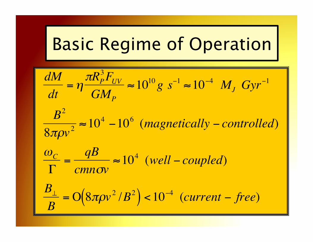
Basic Regime of Operation
€
dMdt
=ηπRP
3FUVGMP
≈1010g s−1 ≈10−4 MJ Gyr−1
B2
8πρv 2≈104 −106 (magnetically − controlled)
ωC
Γ=
qBcmnσv
≈104 (well − coupled)
B⊥
B=Ο 8πρv 2 /B2( ) <10−4 (current − free)
TWO COUPLED PROBLEMS
• LAUNCH of the outflow from planet • PROPAGATION of the outflow in the joint
environment of star and planet, including gravity, stellar wind, stellar magnetic field
• Matched asymptotics: Outer limit of the inner problem (launch of wind) provides the inner boundary condition for the outer problem (propagation of wind)
This Work Focuses on Launch of the Wind

Construct Coordinate Systems that follow Magnetic Field Lines
€
Scale Factors : h j = ε j
−1
Unit Vectors : ˆ e j = ε p h j = e j h j
−1
€
Basis Vectors
coνariant :ε p =∇p
ε q =∇q
contraνariant : e p = ∂
r /∂p
e q = ∂ r /∂q
€
coordinates : (p, q, ϕ)

The Coordinate System
€
B = BP ξ−3 3cosθ ˆ r − ˆ z ( )[ ] + B∗(R∗ /ϖ )3 ˆ z
p = βξ − ξ−2( )cosθ q = βξ2 + 2 /ξ( )1/ 2sinθ
where β = (B∗R∗3 /ϖ 3) /BP ≈10−3 and ξ = r /R∗
∇p = f (ξ)cosθ ˆ r − g(ξ)sinθ ˆ θ
∇q = g(ξ)sinθ ˆ r + f (ξ)cosθ ˆ θ [ ] g−1/ 2(ξ)
where f = β+ 2ξ−3 and g = β − ξ−3

Magnetic Field Configuration
0 2 4 6 8 10
OPEN FIELD LINES
CLOSED FIELD LINES
Magnetic field lines are lines of constant coordinate q. The coordinate p measures distance along field lines. Field lines are open near planetary pole and are closed near the equator. Fraction of open field lines:
€
f =1− 1− 3β1/ 3
2 + β
⎡
⎣ ⎢
⎤
⎦ ⎥
1/ 2
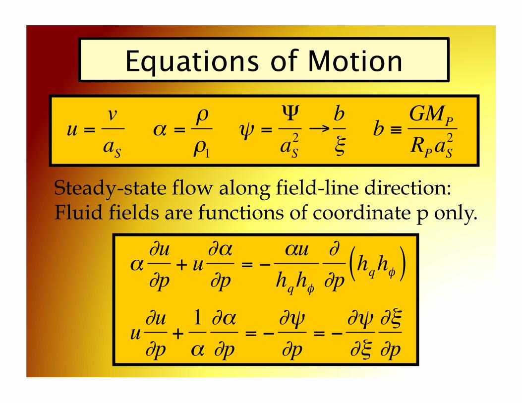
Equations of Motion
€
α∂u∂p
+ u∂α∂p
= −αuhqhφ
∂∂p
hqhφ( )
u∂u∂p
+1α∂α∂p
= −∂ψ∂p
= −∂ψ∂ξ
∂ξ∂p
Steady-state flow along field-line direction: Fluid fields are functions of coordinate p only.
€
u =vaS
α =ρρ1
ψ =ΨaS2 →
bξ
b ≡ GMP
RPaS2
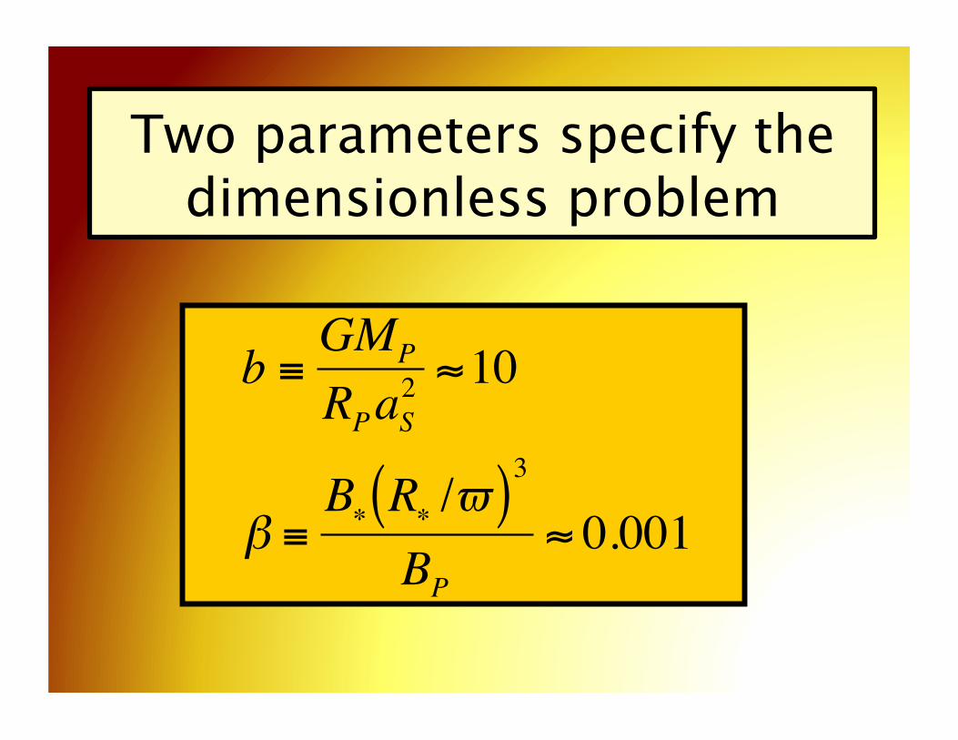
Two parameters specify the dimensionless problem
€
b ≡ GMP
RPaS2 ≈10
β ≡B∗ R∗ /ϖ( )3
BP
≈ 0.001

Solutions
€
b3
=2 f 2 − g2 / f + 2g + 2 f( )q2 /ξ2
f 3ξ2 + g2 − f 2( )q2
λ = qHS−1/ 2 exp λ2H1
2q2+bξS− b − 1
2⎡
⎣ ⎢
⎤
⎦ ⎥
f = β+ 2ξ−2, g = β − ξ−3, and
H = f 2 cos2θ + g2 sin2θ, sin2θ = q2 /(βξ2 + 2 /ξ)
Sonic point
Continuity eq. constant
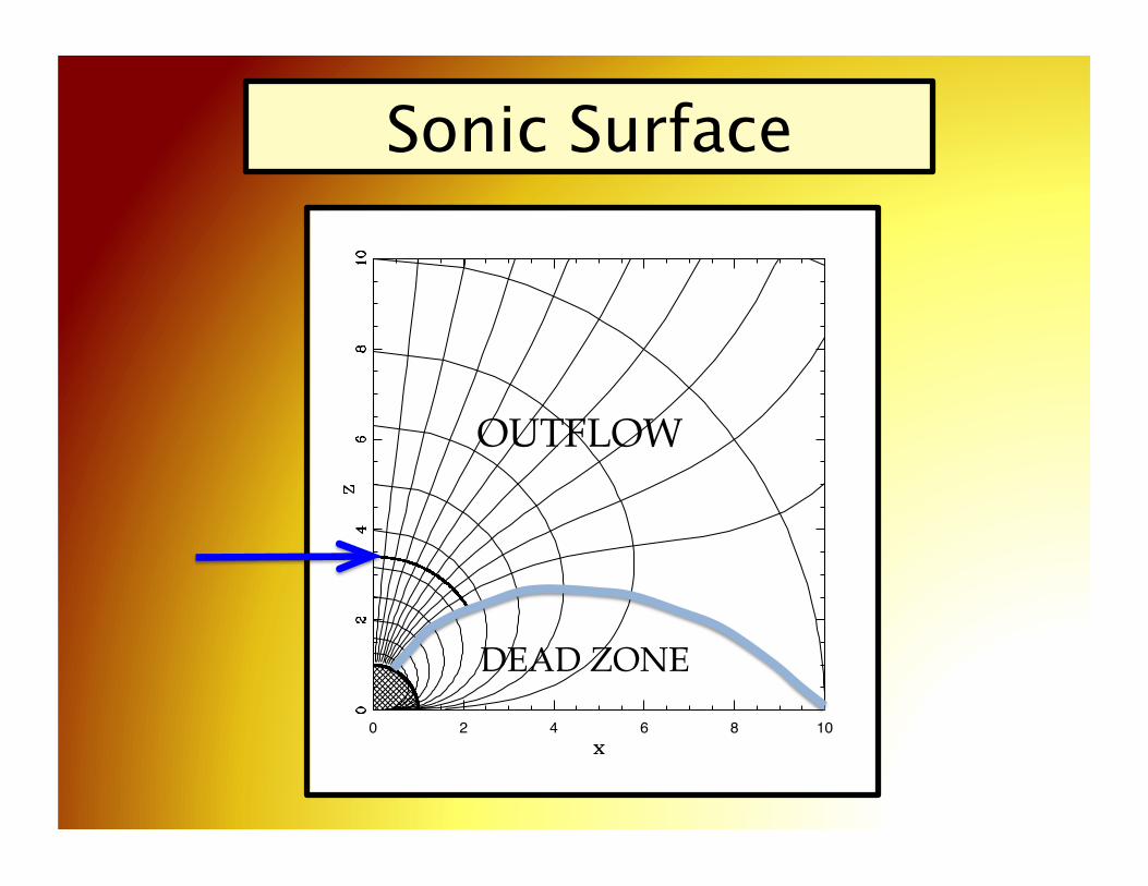
Sonic Surface
0 2 4 6 8 10
OUTFLOW
DEAD ZONE
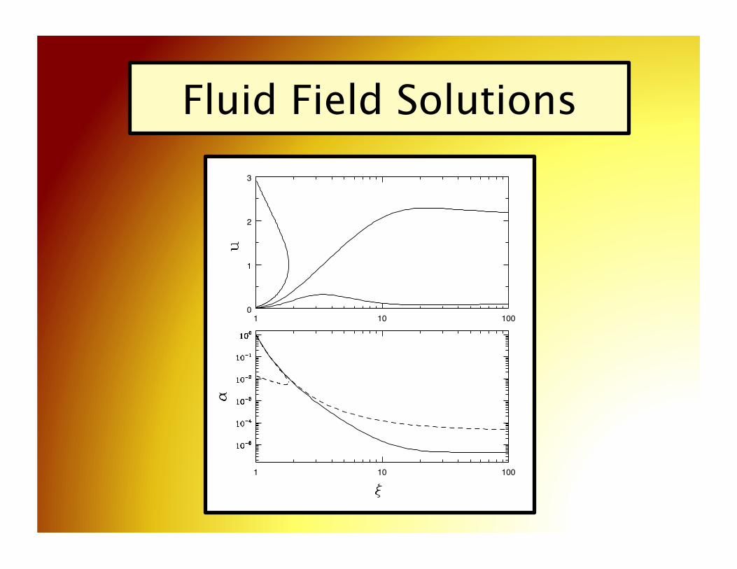
Fluid Field Solutions
1 10 1000
1
2
3
1 10 100
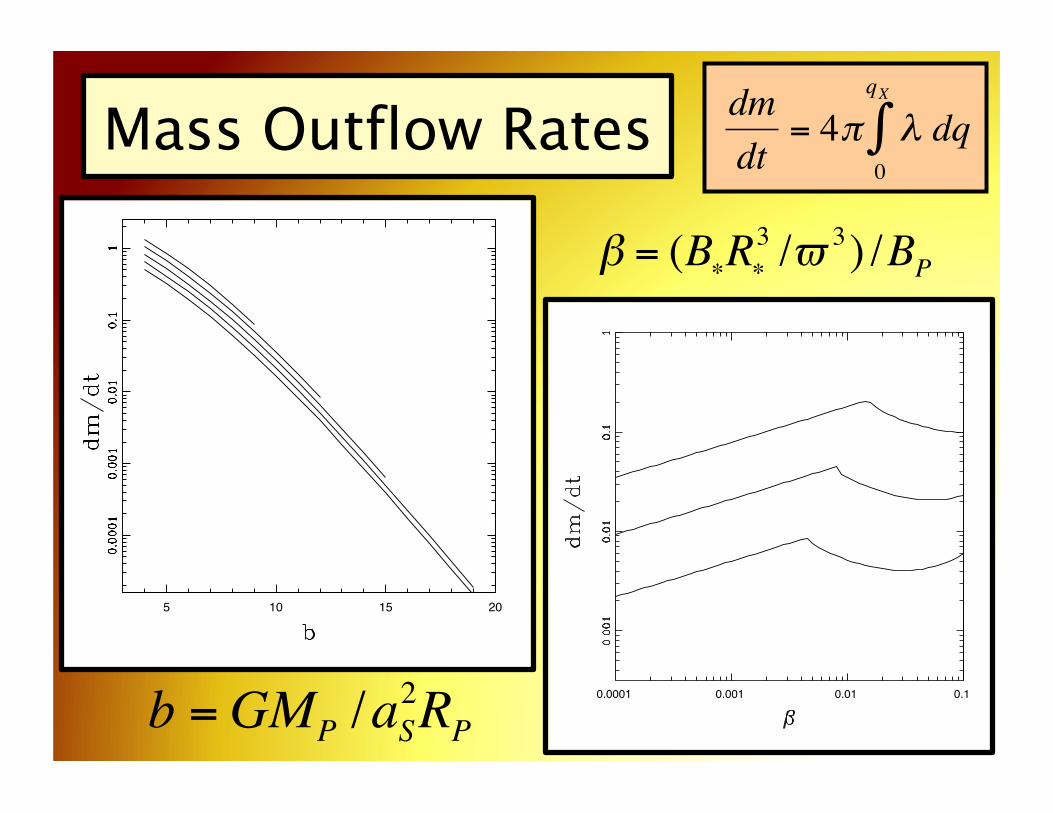
Mass Outflow Rates
5 10 15 20
0.0001 0.001 0.01 0.1
€
b =GMP /aS2RP
€
β = (B∗R∗3 /ϖ 3) /BP
€
dmdt
= 4π λ dq0
qX
∫

Mass Outflow Rates
5 10 15 20
0.0001 0.001 0.01 0.1
€
b =GMP /aS2RP
€
β = (B∗R∗3 /ϖ 3) /BP
€
dmdt
≈ A0 b3 exp −b[ ] β1/ 3
where A0 ≈ 4.8 ± 0.13

Physical Outflow Rate vs Flux
€
MP = 0.5, 0.75, 1.0MJ

Column Density
0 2 4 6 8 10
€
τUV =1

Observational Implications
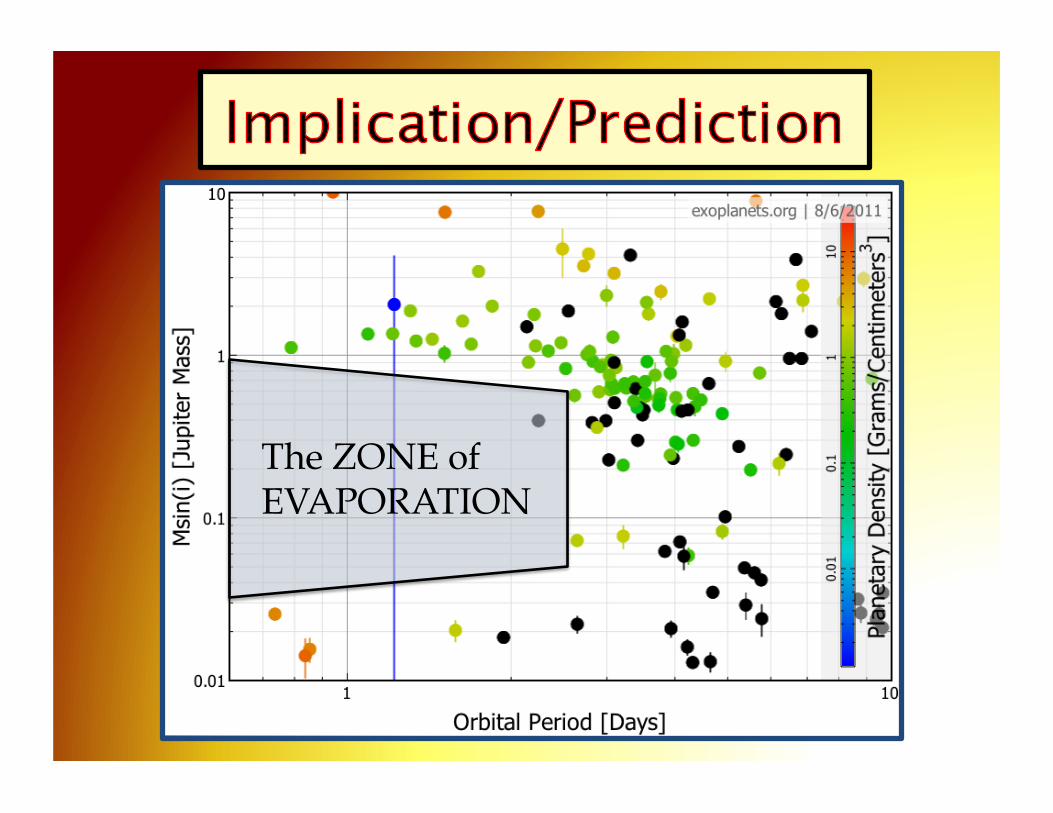
The ZONE of EVAPORATION
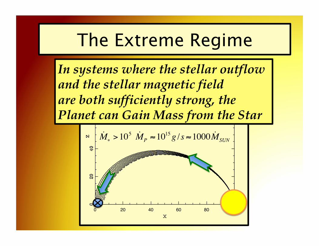
The Extreme Regime
0 20 40 60 80 100
In systems where the stellar outflow and the stellar magnetic field are both sufficiently strong, the Planet can Gain Mass from the Star
€
˙ M ∗ >105 ˙ M P ≈1015 g /s ≈1000 ˙ M SUN

Summary 1.0• Planetary outflows magnetically controlled • Outflow rates are moderately *lower* • Outflow geometry markedly different: Open field lines from polar regions Closed field lines from equatorial regions • In extreme regime with strong stellar outflow
the planet could gain mass from the star • Outflow rates sensitive to planetary mass:
(F. C. Adams, 2011, ApJ, 730, 27)
€
˙ m ∝ b3 exp −b[ ] β1/ 3, b = GMP /(aS2RP )

• Most material that ends up in a forming star is processed through the disk; final accretion flow occurs via magnetic field
• T Tauri star/disks systems observed to have Octupole and Dipole Magnetic Fields, and support Transonic Flow onto Star
• Want to understand the sonic transition for magnetically controlled flows in general
(F. Adams & S. Gregory, 2012, ApJ, 744, 55)

The Star/Disk System
0 5 10 15
€
B∗ ≈1000 − 3000 G
€
RT = 5 −10 R∗
€
M∗ ≈ 0.5 Msun
disk

Basic Regime of Operation
€
dMdt
≈10−7 −10−8 Msun yr−1
B2
8πρv 2≈ 350 − 3000 (magnetically − controlled)
ωC
Γ=
qBcmnσv
≈104 −105 (well − coupled)
B⊥
B=Ο 8πρv 2 /B2( ) <10−3 (current − free)

Equations of Motion
€
∇ • ρ u ( ) = 0 P = K ρ1+1/ n
u •∇ u +∇Ψ+1ρ∇P +
Ω ×
Ω × r ( ) = 0
B = κ ρ
u where κ = const
Steady-state flow, polytropic equation of state:

To a man with !a hammer,
everything looks like a nail

Dimensionless Equations of Motion
€
α∂u∂p
+ u∂α∂p
= −αu
hqhφ∂∂p
hqhφ( )
u∂u∂p
+α1/ n
α∂α∂p
−ωξsinθ ∇p −1 ˆ x ⋅ ˆ p ( ) = −∂ψ∂p
Steady-state flow along field-line direction, Fluid fields are functions of coordinate p only:
€
ξ ≡r
R∗
, u ≡ | u |
aS
, α ≡ρρ1, ψ ≡
ΨaS2 , b ≡ GMP
R∗aS2 , ω ≡
ΩR∗
aS
⎛
⎝ ⎜
⎞
⎠ ⎟
2
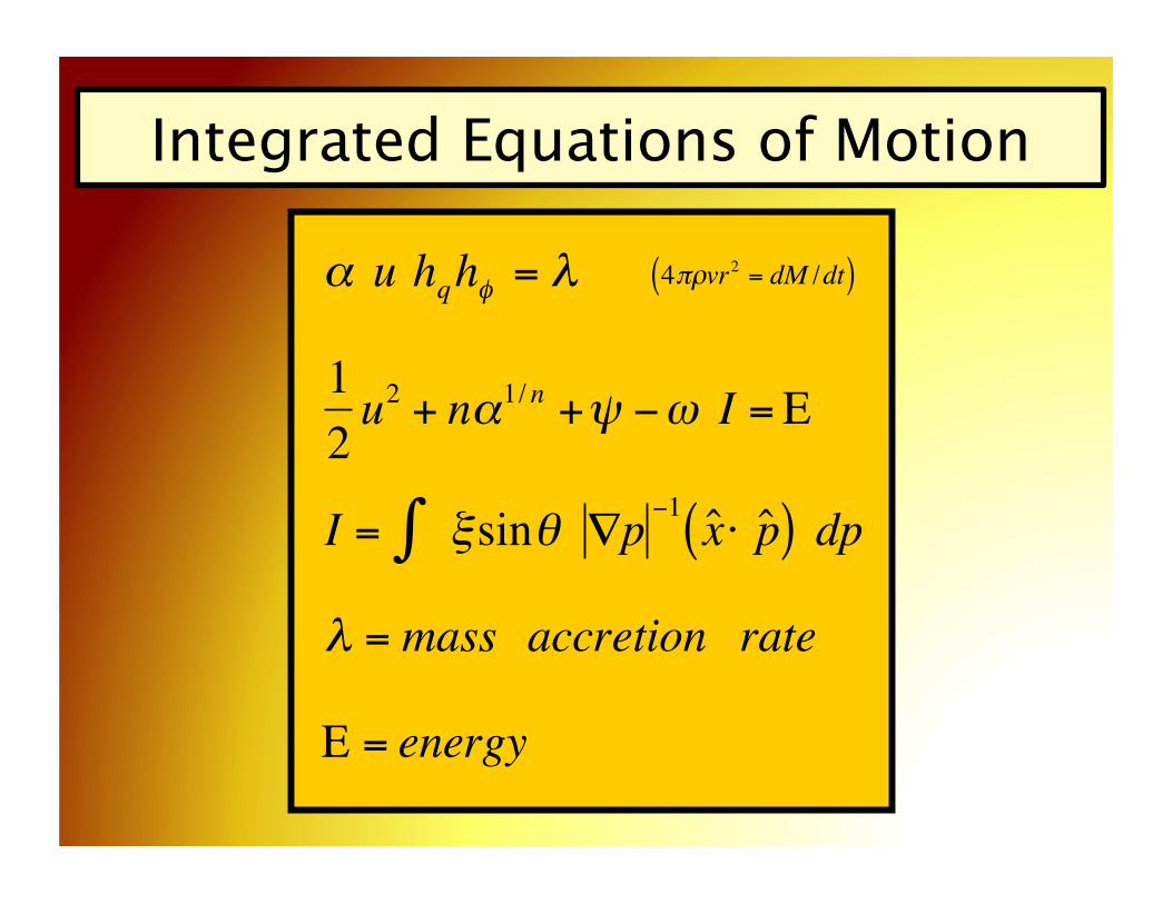
Integrated Equations of Motion
€
α u hqhφ = λ
12
u2 + nα1/ n +ψ −ω I =Ε
I = ∫ ξsinθ ∇p −1 ˆ x ⋅ ˆ p ( ) dp
λ = mass accretion rate
Ε = energy
€
4πρvr2 = dM /dt( )
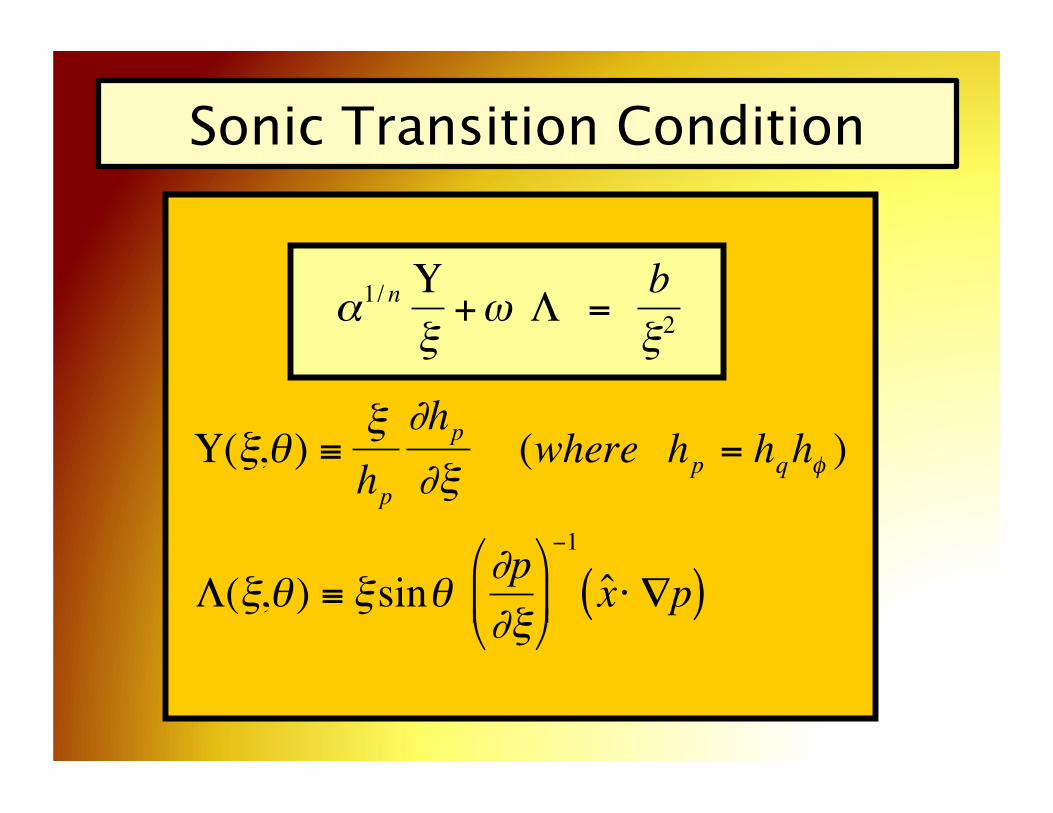
Sonic Transition Condition
€
α1/ n Υξ
+ω Λ =bξ2
Υ(ξ,θ ) ≡ ξhp
∂hp
∂ξ(where hp = hqhφ )
Λ(ξ,θ ) ≡ ξsinθ ∂p∂ξ
⎛
⎝ ⎜
⎞
⎠ ⎟
−1
ˆ x ⋅ ∇p( )€
α1/ nΥξ
+ω Λ =bξ2

reduce to old/known result:
€
α1/ nΥξ
+ω Λ =bξ2
Shu (1992) Gas Dynamics, p. 346 :
n→∞, ω →0, Υ →2 ⇒ 2 =bξ
€
α1/ nΥξ
+ω Λ =bξ2
→ ξs=b2

Score Card
€
b and ω : system parameters (n→∞)
λ and Ε : conserved quantities
Υ(ξ,θ ) and Λ(ξ,θ ) : functions thatspecify magnetic field geometry
field lines ⇒ q = const ⇒ θ = F(ξ)
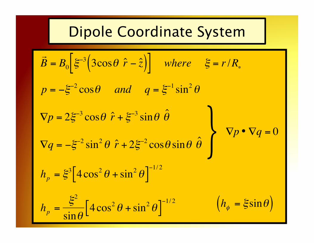
Dipole Coordinate System
€
B = B0 ξ
−3 3cosθ ˆ r − ˆ z ( )[ ] where ξ = r /R∗
p = −ξ−2 cosθ and q = ξ−1 sin2θ
∇p = 2ξ−3 cosθ ˆ r + ξ−3 sinθ ˆ θ
∇q = −ξ−2 sin2θ ˆ r + 2ξ−2 cosθ sinθ ˆ θ
hp = ξ3 4cos2θ + sin2θ[ ]−1/ 2
hp =ξ2
sinθ4cos2θ + sin2θ[ ]−1/ 2
€
∇p •∇q = 0
€
}
€
hφ = ξsinθ( )
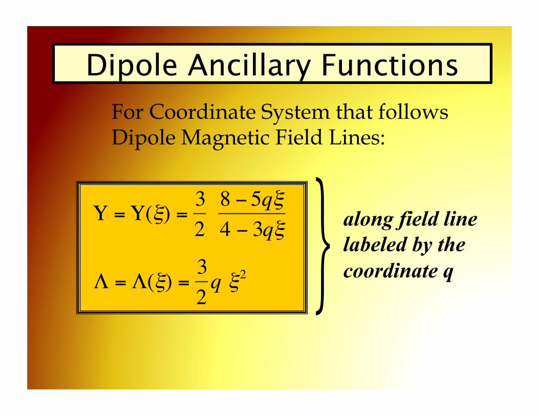
Dipole Ancillary Functions
€
Υ =Υ(ξ) =328 − 5qξ4 − 3qξ
Λ = Λ(ξ) =32q ξ2
For Coordinate System that follows Dipole Magnetic Field Lines:
along field line labeled by the coordinate q
€
}
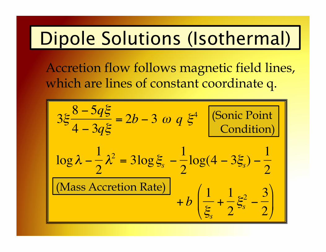
Dipole Solutions (Isothermal)
€
3ξ 8 − 5qξ4 − 3qξ
= 2b − 3 ω q ξ4
logλ − 12λ2 = 3logξs −
12log(4 − 3ξs) −
12
+ b 1ξs
+12ξs2 −32
⎛
⎝ ⎜
⎞
⎠ ⎟
(Sonic Point Condition)
(Mass Accretion Rate)
Accretion flow follows magnetic field lines, which are lines of constant coordinate q.
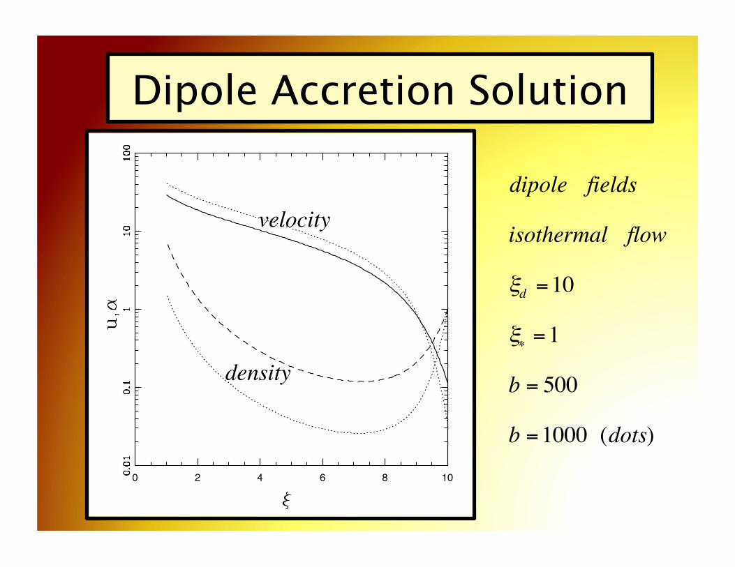
Dipole Accretion Solution
0 2 4 6 8 10
€
dipole fields
isothermal flow
ξd =10
ξ∗ =1
b = 500
b =1000 (dots)
€
velocity
€
density
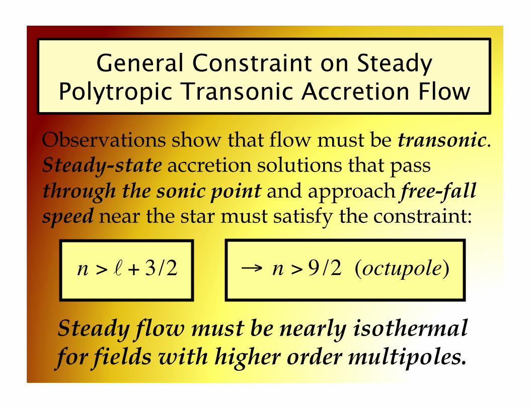
General Constraint on Steady Polytropic Transonic Accretion Flow
Observations show that flow must be transonic. Steady-state accretion solutions that pass through the sonic point and approach free-fall speed near the star must satisfy the constraint:
€
n > + 3/2
Steady flow must be nearly isothermal for fields with higher order multipoles.
€
→ n > 9 /2 (octupole)

Dipole + Octupole Configuration
€
Γ = Boct /Bdip =10
Disk
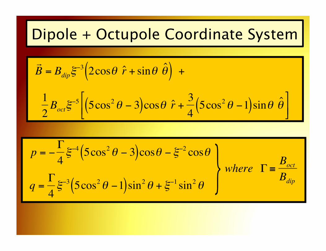
Dipole + Octupole Coordinate System
€
p = −Γ4ξ−4 5cos2θ − 3( )cosθ − ξ−2 cosθ
q =Γ4ξ−3 5cos2θ −1( )sin2θ + ξ−1 sin2θ
€
B = Bdipξ
−3 2cosθ ˆ r + sinθ ˆ θ ( ) +
12
Boctξ−5 5cos2θ − 3( )cosθ ˆ r + 3
45cos2θ −1( )sinθ ˆ θ
⎡
⎣ ⎢ ⎤
⎦ ⎥
€
where Γ ≡Boct
Bdip
€
}

Dipole + Octupole Coordinate System
0 5 10 15
€
Γ = Boct /Bdip =10

Dipole + Octupole Scale Factors
€
hp = ξ5 [ f 2 cos2θ + g2 sin2θ]−1/ 2
hq = ξ4 (sinθ )−1 [ f 2 cos2θ + g2 sin2θ]−1/ 2
where f = Γ (5cos2θ − 3) + 2ξ2
and g = (3/4)Γ (5cos2θ −1) + ξ2
€
sin2θ =25Γ
(ξ2 +Γ) − (ξ2 +Γ)2 − 5Γqξ3[ ]1/ 2⎧ ⎨ ⎩
⎫ ⎬ ⎭
so that f , g, hp , hq = Function(ξ only)

Ancillary Functions for Dipole + Octupole Configuration
€
Λ(ξ) =3ξ5Γ
1+g(ξ)f (ξ)
⎧ ⎨ ⎩
⎫ ⎬ ⎭ (ξ2 +Γ) − (ξ2 +Γ)2 − 5Γqξ3[ ]1/ 2⎧ ⎨ ⎩
⎫ ⎬ ⎭
Υ(ξ) = 5 − f 2 + (g2 − f 2) 15Γ(2ξ2 + 2Γ− f )
⎡
⎣ ⎢ ⎤
⎦ ⎥ −1 ξ5Γ
×
5Γf fξ + g3 fξ4
− ξ⎛
⎝ ⎜
⎞
⎠ ⎟ − f fξ
⎡
⎣ ⎢
⎤
⎦ ⎥ (2ξ2 + 2Γ− f ) + (g2 − f 2) 2ξ −
fξ2
⎛
⎝ ⎜
⎞
⎠ ⎟
⎧ ⎨ ⎩
⎫ ⎬ ⎭
0 2 4 6 8 10
€
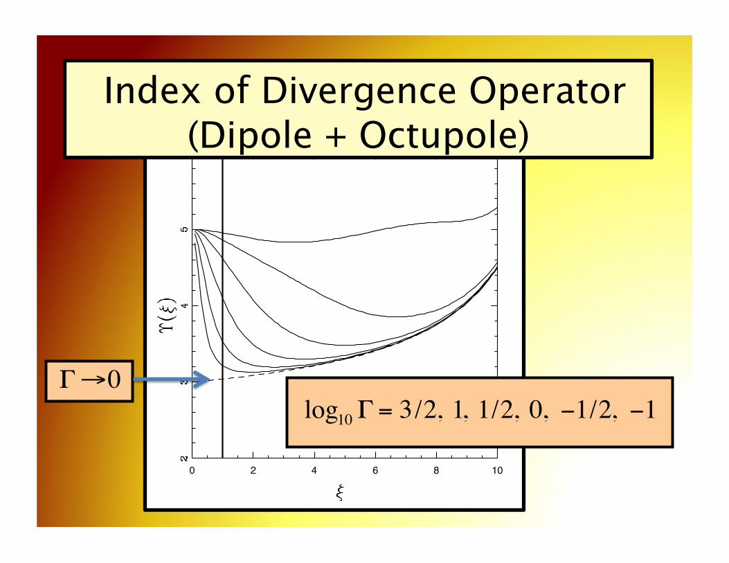
log10Γ = 3/2, 1, 1/2, 0, −1/2, −1
€
Γ→0
Index of Divergence Operator (Dipole + Octupole)

Accretion Solution (Dip+Oct)
0 2 4 6 8 10
€
isothermal flow
octupole Γ =10
ξd =10
ξ∗ =1
b = 500
dots = dipole solution
dashes = full solution
€
velocity
€
density
€
{Density changes by order of magnitude
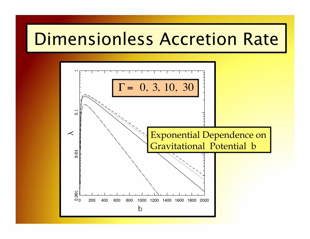
Dimensionless Accretion Rate
0 200 400 600 800 1000 1200 1400 1600 1800 2000
€
Γ = 0, 3, 10, 30
Exponential Dependence on Gravitational Potential b

0 2 4 6 8 10
Dipole + Split-Monopole
0 5 10 15
€
β = 1/4
€
p = −ξ−2 cosθ − βξ−1
q = ξ−1 sin2θ − βcosθ
where β ≡ 2Brad /Bdip
€
β = 2, 1,...1/32

Summary 2.0• Construction of coordinate systems (p,q) • Generalizes to many astrophysical problems • Can find sonic points and dimensionless
mass accretion rates analytically • Dipole + Octupole system: flow density (10x)larger, hot spot has higher temperature • Magnetic truncation radius changes • General constraint on steady transonic flow:
(Adams & Gregory, 2012, ApJ, 744, 55)
€
n > + 3/2 ⇒ nearly isothermal
Dragons
• This use of coordinate systems in this context only works for potential fields (no currents in the flow region) • The formalism has been developed for
two-dimensional systems; can work for three-dimensional systems in principal, but complicated in practice • Treatment (thus far) limited to steady-
state (time independent) magnetic fields: magnetostatics not MHD
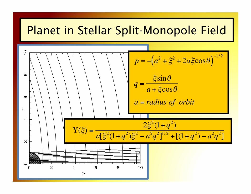
Planet in Stellar Split-Monopole Field
€
p = − a2 + ξ2 + 2aξcosθ( )−1/ 2
q =ξsinθ
a + ξcosθa = radius of orbit
€
Υ(ξ) =2ξ2(1+ q2)
a[ξ2(1+ q2)ξ2 − a2q2]1/ 2 + [(1+ q2) − a2q2]

Parker Spiral in Equatorial Plane
€
p = A log 1− 1ξ
⎛
⎝ ⎜
⎞
⎠ ⎟ + φ
q = ξ −1− logξ − Aφ
A ≡Vwind /(ωR∗) ≈100
(A sets shape of spiral)
-200 0 200

