observations of thermospheric neutral winds by the ucl doppler imaging system at kiruna in northern...

Journal of Atmosyhrric und Terrtwrial Physics, Vol. 50, No. IO/l 1, pp. 861L888, 1988. 0021-9169/88 $3.00+ .OO

Printed in Great Ihitain. Pergamon Press plc

Observations of tbermospheric neutral winds by the UCL Doppler imaging system at Kiruna in northern Scandinavia

S. BATTEN, D. F&ES, D. WADE

Department of Physics and Astronomy, University College London, Gower St., London WClE 6BT, U.K.

and

A. STEEN

Kiruna Geophysical Institute, Kiruna, S-98127, Sweden

(Rucriwdjor publicnlion 20 May 1988)

Abstract-Since the 1982/1983 winter, the UCL group, in collaboration with the Swedish Institute for Space Physics (previously Kiruna Geophysical Institute), has operated a Doppler imaging system at the high latitude station of Kiruna (67”N, 22”E). The Doppler imaging system is an imaging Fabry-Perot interferometer of 13.2 cm aperture. This instrument has been operated on a ‘campaign’ basis for mapping thermospheric winds using the 01 emission at 630 nm (240 km altitude) from a region up to about 400 km radius about Kiruna. In November 1986, the performance of this wide-field Doppler imaging system was augmented by improvements to the detector and all-sky optics. We present data from December 1986, obtained during periods with both clear skies and active aurora1 and geomagnetic conditions. Maps of the neutral wind flow within the auororal oval during disturbed conditions and near magnetic midnight show continuous and rapid changes of thermospheric winds. The typical scale sizes of eddies observed within the mean flow around magnetic midnight are 10&300 km, with fluctuations at all time scales resolved by the 10 min between successive Doppler images. The local and short period fluctuations appear to be a filtered response of the thermosphere to rapid local variations of the convection and precipitation patterns, within a background of global scale changes.

1. INTRODUCTION

Regions of the polar thermosphere which are directly

affected by ion drag forcing and strong heating, by a combination of aurora1 precipitation and Joule heating, will undergo rapid changes of thermospheric temperature, wind and neutral composition. These changes occur on a variety of spatial and temporal scales, similar to the structures and variability of polar, magnetospheric convective electric fields and aurora1 electron precipitation. However, the thermospheric response to localised strong forcing is filtered and damped ; intrinsic properties of its inertia and high viscosity. It also responds as a buoyant, somewhat non-linear fluid under the condition of a rotating planetary atmosphere, one which is also driven by larger scale energy inputs from solar UV and EUV, by large scale energy and momentum forcing from the magnetosphere and by the propagation of certain types of waves and tides from their origin in the lower atmosphere. The observed response of the upper thermosphere is thus considerably modified from the spatial and temporal morphology of the

localised aurora1 forcing. Our basic understanding of the structure and dynamics of the thermosphere, the major physical processes, and a synopsis of recent experimental and theoretical/modelling results is well summarised in a number of the papers presented in this special CEDAR issue.

Great increases in understanding the dynamical response of the thermosphere and particularly that of the polar regions, have come from the combination of both ground based and space borne observations during the past decade. A greatly improved performance of ground based interferometers has been obtained as the result of advances in detector and electronic/computing systems. It has also become rather easier to deploy such advanced instruments from a number of stations in the vicinity of the aurora1 oval and polar cap. A considerable volume of thermospheric wind data is now available from single stations and from a number of important multi- station studies. The Fabry-Perot interferometer (FPI) (HAYS et al., 1981, 1984; KILLEEN et al., 1982; REES

et al., 1983) and the Wind and Temperature sensor (WATS) (SPENCER et al., 1981) of the Dynamics

861

862 S. BATTEN, D. REES, D. WADE and A. STEEN

Explorer-2 spacecraft carried thermospheric dynami- cations (HERNANDEZ, 1986). Field-widening this cal mapping into a truly global phase. In addition to instrument is not simple. Multiple aperture or mul- the global data obtained from DE-2, a number of tiple annulae masks, mounted in the image plane, have important coordinated ground based/spacecraft stud- been used with a photomultiplier with some success ies have also been reported (for example, KILLEEN et (SHEPHERD et al., 1965, 1978 ; STIPLER and BIONDI, al., 1986 and REES et al., 1985, 1986). In combination 1978). This technique has been shown to increase the these studies have lead to a much improved picture of etendue by up to a factor of about 5, allowing for both the overall climatology of thermospheric dynam- transmission losses within the mask. However, the ics and on its ‘meteorological’ variations with spatial physical alignment of such masks is critical, it is scales of several hundred km and with time scales difficult to maintain a high finesse and relatively few down to the order of l&30 min. instruments have been regularly used.

The wind data obtained from the middle and upper thermosphere of the highest quality, time and spatial resolution has always hinted that, against a background of medium to global scale flows (say 1000 km and upward), many very interesting phenomena occurred with smaller spatial scales (lo&-500 km) and with correspondingly shorter time scales (down to 10 min, or approximately the Brunt-V&G frequency). Several types of observed wind variations have indicated strong correlations with locally intense ion drag and Joule and particle heating during excep- tional aurora1 events, in addition to the forcing of large scale polar thermospheric flows by the twin cell ion convection patterns at high geomagnetic latitudes (i.e. &ES et al., 1983; HAYS et al., 1984).

A number of ‘second generation’ Fabry-Perot interferometers have used imaging detectors to obtain a full image of approximately 1.5 complete interference orders so that a complete image of the line is obtained, irrespective of where it appears within a given free spectral range. This increases the etendue by approximately the overall finesse of the interferometer (REEs et al., 1982; KILLEEN et al., 1983). This is normally a factor of about 12 for applications involv- ing observations of atmospheric emissions of the 01 630 nm line. Since airglow signals are always weak, data analysis accuracy is always photon limited. It is thus essential that low noise imaging detectors are used to increase the effective instrument throughput.

It has been difficult to resolve short period wind fluctuations with the traditional Fabry-Perot interferometer (HERNANDEZ, 1986 ; SMITH and SWEENEY, 1980). With this in mind, the concept of obtaining improved sensitivity and thus better accuracy and time resolution, by field-widening a Fabry-Perot interferometer beyond the traditionally pin-hole detector, or the single fringe used with a number of second generation FPI’s (REES et al., 1982), has been attractive.

The major observational difficulty is the relatively low signal available from the sky during average aur- oral conditions, rather than at times of exceptionally bright aurora. There is a practical maximum aperture to the Plane Fabry-Perot instrument of about 15 cm. This is dictated partly by cost, partly by the limited availability of material of suitable optical quality at larger sizes and partly by the difficulty of designing suitable mechanical mountings to constrain the etalon plates without distortion. Since maximum aperture is essentially fixed, solid angle is one other ‘free’ par- ameter which may be increased. The other free parameters, detector detective quantum efficiency and filter transmission, have been at the limits of the appropriate state of the art for some years.

Beyond this factor of about 12 gain, the only other possible way to increase the overall instrument sensitivity is to increase the number of Fabry-Perot fringes which are imaged simultaneously. This is not a trivial requirement since it is necessary to ensure that positional information (i.e. fringe location or diameter) is not degraded, since this would inevitably lead to a loss of wind speed accuracy. An increase in sensitivity could be used to decrease the time required to obtain a valid measurement with the instrument pointing in a given direction. A greater number of individual measurement directions, or a faster cycle time (better time resolution), could be obtained, com- pensating for this sensitivity increase.

Instead of this possible gain, we have chosen to attempt to image most of the sky through the field- widened interferometer (&ES and GREENAWAY,

1983). The all-sky image (related to the optical system of a conventional all-sky camera) can be dissected, rather like the segments of an orange. Each of a number of consecutive fringes can be used to define a series of radial positions at which an independent Doppler shift can be obtained.

A traditional Fabry-Perot interferometer has an on-axis aperture (pin-hole), and a photomultiplier is normally used as the detector for low light level appli-

In practice, since the available signal is always ‘photon-limited’ and because the spatial resolution is limited by the capabilities of the imaging detector and usable computer memory, it is not possible to carry out and divide the fringes into an infinite number of sectors. It is also only possible to use a finite number

Observations of therrnospheric neutral winds 863

of fringes. Indeed, much of the past 3 years has been spent iterating the optical design to find the optimum number of fringes and fringe segments which could be efficiently observed given the known resolution limitations of our imaging photon detectors (IPD, MCWHIRTER et al., 1982). At present, 5 or 6 individual F-P fringes are used, imaged onto about 140” arc of the sky. Twenty-four independent radial segments (15” sectors) are used for analysis of azimuthal information.

Within the confines of this paper we will not com- pare in detail the performance of the Doppler imaging system with that of the field-widened Michelson interferometer (WAMDII-WIENS et al., 1987). That instrument, in its somewhat different forms, is quite complex. The field-widened Michelson requires a spectral scan of the interferometer over the entire image plane. The method provides direct spectral imaging of all discrete picture elements in the image plane, but with a low finesse (2 wave interferometry of the Michelson). Normally, the Michelson is physically scanned (capacitance stabilised piezo-electric trans- ducers) to sample the spectrum at 4 points within the free spectral range.

We have chosen to perform the spectral scan at much higher finesse (instrument finesse = 16, overall finesse for 01 630 nm = 6). In essence, however, only some 5 * 24 (120) individual elements are available within our scheme. For 01 630 nm our method provides a good technique for separating spatial and temporal variations in the intensity of the spectral emissions from true spectral variations. The DIS is not sensitive to temporal variations, since the signal is integrated at all picture and spectral elements over the same time period. For the thermospheric 01 630 nm emission, the spatial variations of intensity are almost always gradual on the scale of the individual sample points. For emissions such as 01 557.7 nm, or the prompt N: emissions, the sharp spatial fluctuations could cause ambiguities in the spectral analysis. Data obtained with a field-widened Michelson is always prone to ambiguities caused by rapid temporal variations of intensity during the period of individual spectral scans. These can be minimised by adding the data from a number of consecutive spectral scans and it is possible to maintain a short individual integration period as a result of its very large throughput.

2. INSTRUMENTATION

The general principles of the optical system of the Doppler imaging system (DIS), and of the appropriate data analysis methods, have been previously described

by REEK and GREENAWAY (1983). REES et al. (1984) described some preliminary data obtained during December 1983 by the prototype DIS operated at Kiruna Geophysical Institute (now the Swedish Insti- tute for Space Physics), at a time of an unusually large geomagnetic disturbance.

The major principle of the Doppler imaging system is that a conventional Fabry-Perot interferometer of high spectroscopic resolution is modified in two ways. Firstly, a high resolution, two-dimensional, imaging photon detector (IPD, MCWHIRTER et al., 1982) is used in the focal plane to record the images of about 5 or 6 individual Fabry-Perot fringes. Secondly, a wide-angle (all-sky) optical system is placed ahead of the Fabry-Perot etalon, to match a wide field of view (some 120” arc, full angle) to the field of view of the F-P fringes in the focal plane (about 2.5” arc, full angle). In this way, individual sectors of individual F-P fringes correspond to quite widely separated regions of the sky. For an optical emission such as the 01630 nm line, coming from a region centred around 240 km altitude, a typical spatial resolution of the order of 20 to 40 km may be obtained over a region up to around 600-800 km diameter.

Since the initial prototype of the DIS was used in 1983 (K!ZES et al., 1984) the efficiency of the wide- angle optical system has been improved significantly. Of equal, or perhaps even greater importance, the problem of coping with the collection, analysis and interpretation of a very large quantity of data has become nearly bearable. This is partly the result of more powerful computers, such as the IBM PC-AT, which now runs the DIS and a MicroVAX which carries out the major part of the analysis at UCL. Significant progress has also been made in developing improved techniques for processing the Doppler data from the raw F-P fringes.

3. CALIBRATIONS

One of the earliest problems encountered with the DIS was a consequence of seeking high system reliability by avoiding the use of any moving parts within the instrument. It is inconvenient to period- ically view a spectral calibration lamp. The early data was thus rather difficult to analyse, except at times of very high thermospheric winds (REFS et al., 1984) since very small instabilities of the etalon gap, induced by temperature changes or errors or drifts in the IPD signal processing electronics etc., could not be regularly calibrated. A practical, if imperfect, solution to this problem is the continuous illumination of a small

864 S. BATTEN, D. REFS, D. WADE and A. STEEN

portion of the optical dome, through which the DIS views the sky, using a neon calibration lamp (630.4 nm line). This R-F powered lamp produces a strong and convenient line which is transmitted by the interference filter used for isolating the 01630 nm line.

The spectral calibration ‘patch’ within each and every Doppler image provides an essential facility for calibrating the etalon and entire system as long as the IPD signal processing electronics system and the mechanical parts of the optical system are very stable. After considerable system testing this appears to be the case.

Other necessary calibrations of the DIS are (REES et al., 1984): (i) flat field sensitivity calibration; (ii) thermionic emission calibration ; (iii) geometric calibration of the image plane against the sky ; (iv) determination of the centroid of the F-P fringe pattern for the reduction to radius.

4. SYSTEM OPERATING SOFI-WARE

The Doppler imaging system shares many of the technical features of the range of single and multiple etalon Fabry-Perot interferometers built and operated by the UCL group (REES et al., 1982, 1986). The lack of a scanning mirror system and the continuous, rather than periodic, operation of the spectral calibration lamp are the major hardware differences which have an impact on the control electronics or software.

As a result of this similarity with the other 5 FPI interferometers, which are in routine operation, the PC operating software is a close derivative of the ‘HAL’ programmes which are the ‘standard’ UCL FPI operating software. The major additional requirement is that the Doppler image can be dissected into 24 sectors, centred on the centre of the Fabry-Perot fringe pattern. Each sector is 15” wide, corresponding to an azimuthal strip of the same width, centred on the local zenith (within the accuracy that the instrument can be set up). The raw image data, initially stored as photon counts for each image pixel, is ‘reduced to radius squared’, providing a spectrum vs. wavelength (256 wavelength elements) for each of the 24 image sectors or segments. These data are then stored on disk, providing a reduction factor of about 10 in the data volume, compared with storing complete 256 * 256 images. The normal integration time is 600 s, so that up to 96 complete reduced Doppler Images have to be obtained and stored each night the system is operated. Near the winter solstice, when the observing night approaches 16 hours, the data stored per night slightly exceeds the capacity of a quad density disk for the IBM PC-AT (1.2 Mb).

5. DATA ANALYSIS

There are several stages of data analysis which will be very familiar to every user of Fabry-Perot systems : the recording of F-P fringes ; their analysis in the presence of a photon limited signal and the deduction of a Doppler Shift; and its conversion into a line of sight velocity.

The differences between the full analysis of the DIS data and previous systems are dealt with conceptually by REES and GREENAWAY (1983). However, at that time, they considered a near-Utopian situation and thus we will summarise the major practical steps in the analysis.

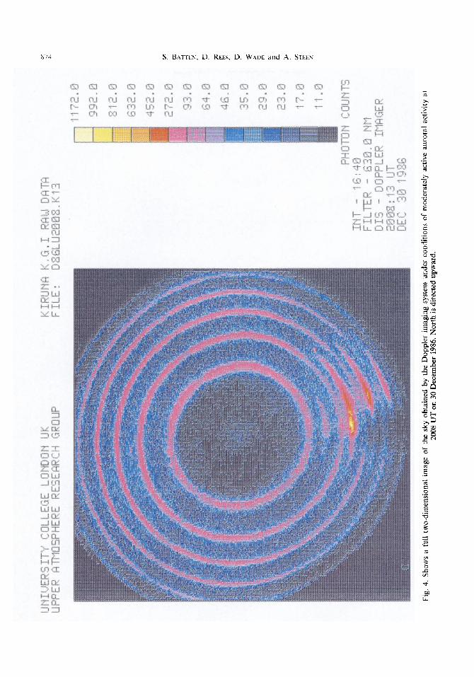
(i) The two-dimensional Fabry-Perot fringes and the associated calibration images are reduced to (radius)2. Spectra are thus produced for each of 24 equal area sectors of 15” arc, about the centre of the F-P fringe pattern (which has to be accurately determined a priori). Each sector in the present configuration contains 5 full free spectral ranges (at 630 nm, 6 at 557.7 nm). For calibration purposes several full 256 * 256 pixel images are also stored (such as that shown in Fig. 4). These full images take a factor of 12 more disk storage than the reduced fringe data and this mode is not used for routine operations to avoid running out of disk space.

(ii) The data from these 24 individual sectors, each of 256 words (or wavelength samples) are stored for subsequent calibration and analysis on a DEC 1 l/23 computer (RL-02 hard disk), or alternatively on a machine such as the IBM PC-AT or COMPAQ-286. Each data file contains a header with a complete description of location, data, time and other necessary background information. A subset of this data is used to create a unique directory entry, which acts as the system log. While a wide range of integration times can be used, in practice, most of the results have been obtained with either a 5 min or a 10 min integration time.

(iii) Two of the 24 sectors contain image data from the calibration lamp, providing the image by image monitor of changes of etalon gap, etc. In practice, such changes are very small but must be monitored to ensure the reliability of the complete DIS system. Data and images from very cloudy periods, when the ‘standard’ UCL FPI at Kiruna shows extended periods of very small Doppler shifts in all directions, is used to provide a best estimate of the ‘zero wind’ fringe locations and of the internal self-consistency of the entire DIS and its data analysis system.

(iv) At UCL, these data are processed to provide fringe peak locations, in conjunction with error esti- mates, 01630 nm intensity data, background intensity

Observations of thermospheric neutral winds 865

data for each of the fringes, and for each of the sectors, for each individual DIS image.

Multiple fringe profile Fourier analysis

With this type of instrument we are interested in measuring a frequency spectrum S(v), which is excited by the source E(v), which has a finite spectral width so that the scattered light spectrum is represented by the convolute of S(V) and E(u). This spectrum is then detected with the Doppler imager whose transmission profile, as a function of frequency, is given by F(v).

The measured data Y(u) is thus an interferogram which is the convolution :

Y(u) = S(u) *E(v) *F(u) (1)

The transmission profile F(v) is in itself the convolute of several instrument qualities as follows :

F(u) = A(u) *D(u) * M(u) * P(v), (2)

where ,4(u) is the ideal etalon Airy function, D(v) is the defect finesse due to curvature, M(c) is the microscopic imperfection effect, P(u) the pixel aperture effects, and since we are dealing with a physical instrument in the real world there is also noise, N(u). which must be added to the profile.

Since convolutions are associative and com- mutative (BRACEWELL, 1965) the full expression for the detected profile can be written in convolution notation as :

Y(u) = S(u)*E(u)*A(u)*D(u)*M(u)*P(u)+N(u) (3)

and since convolution corresponds to multiplication in the Fourier domain (Convolution Theorem, BRACE- WELL, 1965) and addition corresponds to addition in the Fourier domain (Addition Theorem, BRACE~ELL, 1965) this function has the Fourier transform :

y(v) = s(~)*e(v)*a(v)-d(u)-m(u)-p(v)+n(u). (4)

Each of these component functions has been well discussed in the literature (for example COOPER, 1971; HAYS and ROBLE, 1971; HERNANDEZ, 1978 ; KIELKOPF, 1979), along with its appropriate Fourier transform. It has been proved that in the Fourier transform domain, the resultant function is limited to the lower spatial frequencies, whereas the noise N(u) is spread over all frequencies. Thus, the application of a low pass Fourier filter is a valid method for the determination of an analytical fit to the data.

It can be shown that the variables that determine the fall-off of the signal in the Fourier domain are the three instrument parameters : T (transmittance), R

(reflectivity), z (7 = M/c), where d is the etalon gap, n is the order of interference and c = 3 * 10’ ms ’ and the properties of the source AU,, the half-width at half- intensity of the emission, and Au, the half-width at half-intensity of the instrument function.

These values are directly related to the finesse and the etalon gap (d) of the instrument and to the temperature and wavelength of the emission profiles. Thus we need to determine, by calibration, the filter parameters once for each instrument. These values can then be used to analyse all the collected data. The noise will, of course, vary depending on detected intensities, which is dependent on aurora1 activity, etc. However, the signal will never vary outside the filter range. In practice, the critical frequency is determined by consideration of the measured free spectral range (related to z) and the minimum half widths of the detected peaks. This process gives a maximum range for signal detection in the Fourier domain, thus providing a maximum filtering of noise, without a serious loss of true signal information.

Shape qf'the jilter

As stated earlier, lowpass filtering using a tophat function in the Fourier domain, is equivalent to convolving the data with a sine function. For the purposes of this analysis, the sine function has undesirable side lobes which can lead to the ‘Gibbs effect’ (BRACEWJZLL, 1965). To reduce this effect, it is desirable to remove sharp changes in gradient from the chosen lowpass filter.

By trial and error, it was found that the best filter to use was a cosine bell or Hanning filter (KOOPMANS, 1974) with a taper width of 20% of the cut-off frequency. This filter is flat (Xl) out to the cut-off frequency and then falls smoothly to zero along a cosine curve, with no sharp changes in gradient.

Recorery qfanalyticalfunction

The Fourier cosine transform of the data is multiplied by the obtained filter in the analysis suppressing the higher frequencies and thus smoothing the data. The filtered spectrum is then transformed back with the inverse Fourier cosine transform, producing the smoothed fit to the data. This is equivalent to doing a convolution in the radial domain. The filtered Fourier coefficients are retained, since they represent the analytic function as a specific sum of cosine terms and are thus useful for the interpolation of the analytic curve to find the peak position, since they define the curve at all points.

866 S. BATTEN, D. Ram, D. WADE and A. STEEN

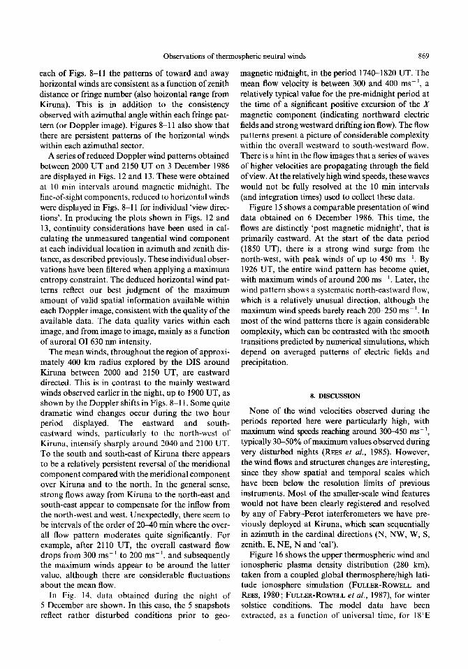
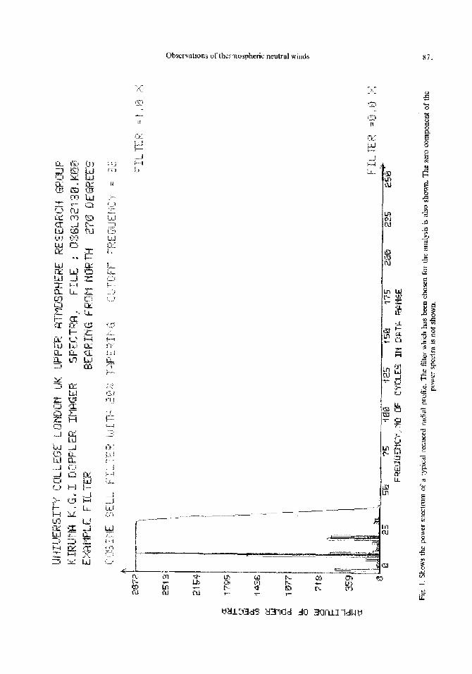
Figure 1 shows the chosen filter, together with the power spectrum of a typical reduced radial profile. The zero component of the power spectrum is not shown, since it tends to be much larger than the remaining frequency components and would alter the scaling of the plot, thus obscuring the detail of the spectra. The first component corresponds to the average level of the radial profile. The Fourier cosine transform of the data is multiplied by the displayed filter in the analysis suppressing the higher frequencies and thus smoothing the data. The noise levels, as seen in the power spectrum, are lower than those in the cosine transform, since the power spectrum is equivalent to the square of the cosine transform.

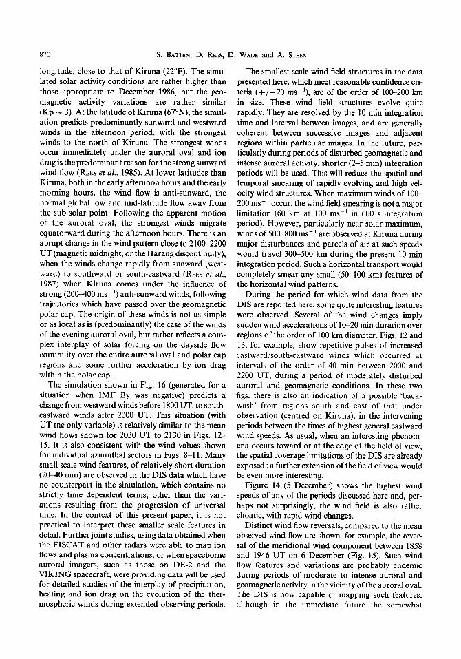
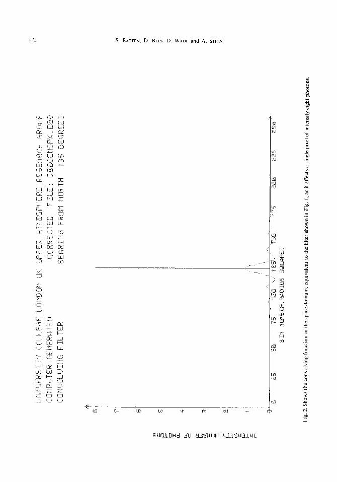
Figure 2 shows the convolving function in the space domain. This is equivalent to the filter shown in Fig. 1, since it affects a single pixel of intensity eight photons. Note that the curve is limited in range and contains the same number of photons as the original pixel.

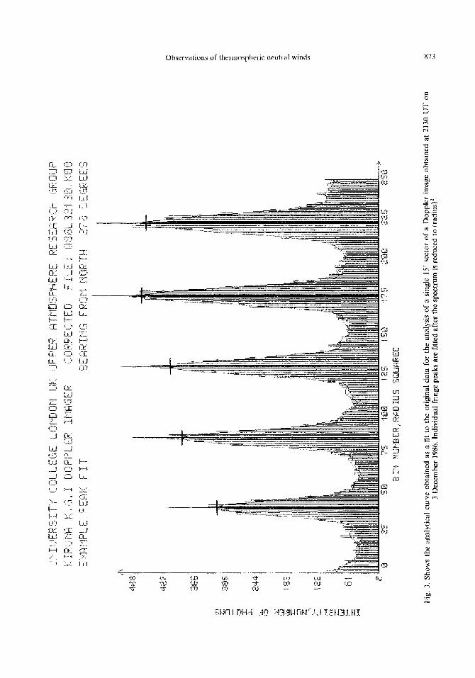
Figure 3 shows the analytical curve obtained as a fit to the original data. Note that not all the noise has been removed since some of the noise was contained in the lower frequencies. However, the majority of the remaining noise is now concentrated in the troughs between the peaks where the signal is low and where noise was dominant in the original data. This causes no real problems, however, since the area of interest for Doppler wind determination is the top half of the peaks. The detected peak positions are also shown.

Determination @“peak position

The fitted curve returned by the analysis is scanned for turning points, which are then subjected to certain checks to see if they correspond to peaks, troughs or noise. There are several checks, some of which can be altered by the user depending on the quality of data available for analysis.

If all these conditions are satisfied an accurate peak position is determined, to an arbitrary precision, by a Newton-Raphson iteration along the analytical curve. The cosine transform coefficients are used to determine the value and differential of the fit at the interpolated points. Thus, the accurate positions of the peaks are determined.

Calculation of wind velocities

The first stage of the calibration is to calculate the period average of the peak positions for each section and fringe. This is done in order to calibrate to the mean wind velocities over a chosen period. One of the sectors returned contains fringes from the calibration

lamp and these should remain in a constant position so changes in the calibration fringe diameter can be attributed to instrumental drift.

The shifts observed in the calibration fringe positions are thus removed from the data in the other sectors to correct for the effects of, for example non- constant etalon temperature.

The averages obtained over long periods (usually 24 h) are attributed to the ‘zero velocity’ fringe position. This has been determined for the instrument, using a combination of spectral calibrations of the full image field and using sky spectra (630 nm) obtained from long sequences of images taken during cloudy periods. At such times, the ‘standard’ UCL Fabry- Perot Interferometer at KG1 indicates low Doppler shifts (a combination of low winds and/or cloudy sky conditions).

The absolute line-of-sight wind velocities, V,, are calculated from the formula :

V,s = c*1/2t (Cal-dat)/fsr, (5)

where V,* is the line of sight wind velocity, c is the speed of light in vacuum, 1 is the wavelength of observed emission, t is the etalon gap, cal is the calibration peak position, dat is the data peak position corrected for instrumental drift, fsr is the free spectral range. The free spectral range cfsr) is equal to the distance between adjacent peak positions.

The Doppler shifts obtained are then corrected to horizontal wind components v,,~, assuming that there is no vertical wind component and that the horizontal wind can thus be derived from the line of sight component, V,* multiplied by set (zenith distance), i.e. :

Vdi,j) = Vdi,A * se44), (6)

where i refers to the azimuthal sample (l-24) and j refers to the fringe number (l-5). Zenith distance, 4, is a precisely calibrated function of the instrument field of view. We assume that since the Doppler shifts are very small in subtended arc angle, both in the image plane and in the projected plane at 240 km altitude, the zenith distance is actually a consistent function of the fringe number and thus ‘diameter’. The major point at this stage, is to demonstrate that there is azimuthal, radial and temporal consistency of the derived wind patterns. To this effect a collection of figures is presented in the next section.

We now have to look at how to best derive the maximum information on real structures of the horizontal wind field from the individual and sequential Doppler images. The horizontal wind components obtained initially can be used to calculate a maximum entropy estimate for the underlying wind field, includ-


ing localised structure. A successful analysis strategy would fully use all the azimuthal, radial and temporal information available to deduce a minimum entropy solution which best represented the horizontal and temporal wind structures. We have to note that the instrument only directly measures the radial wind component. In deriving the non-radial wind component in order to determine the full wind field, we have to give greater weight to actual measured (and thus radial) wind components than to inferred/ calculated azimuthal components.

The influence of analytical errors and photon noise etc. must not be allowed to outweigh the available data quality. In a search for rapid spatial and temporal wind field fluctuations, which is the entire rationale of the DIS, the underlying philosophy has to be to remain within reasonable bounds, which are determined mainly by data quality. However, the pro- cedure has also to be tempered by understanding that unknown and variable vertical wind components may have a very undesirable influence in the interpretation of individual Doppler images, although their influence on ‘average’ results will, or should, be relatively unim- portant.

We wish to couple the data from successive fringes : a strong wind observed at one fringe location at one azimuth angle should be related to similar features observed in adjacent azimuth angles in adjacent fringes and also in previous and subsequent Doppler images (allowing for the significant transport of parcels during a 5 or 10 min interval). The 5 or 10 min observing interval will inherently cause some smearing of Doppler shifts when the horizontal wind is large. Typically, the spatial grid is approximately 80 km. If there is a horizontal wind of more than 200 ms- ’ the wind in adjacent ‘pixels’ along the wind velocity vector should be strongly correlated. If this correlation does not occur, we should suspect that there is a serious difficulty with data quality or with the data analysis process.

Weighted Chebyshev interpolation is used to estimate the vector component of the field in the twelve measured cross field directions. The assumption is then made that the 0 component of the vector field varies only in the 6’ direction and that perturbations in the field in the 4 direction are caused by perturbations resulting in the 4 directions. Thus, twelve one-dimensional component vectors can be estimated for every point in the two-dimensional field corresponding to the twelve measured vector components of the true wind field. This assumption comes directly from New- ton’s second law :

f = d(mv)/dt, (7)

where f (force) and v (velocity) are vector quantities, i.e. the action is in a specified direction. This polar- isation of the vector field is not a unique solution for the data but is the solution which make the least assumptions about unmeasured components (maximum entropy).

The twelve component vectors y., at each point of the field, having now been calculated are assumed to be twelve components of one wind vector as viewed in each of the twelve directions. This assumption is not uniquely valid because of the spatial differences associated with the determination of each vector, but will give the maximum entropy (i.e. smoothest) wind flow pattern consistent with the data. The wind vector is described by the equation :

w= Vcos(6-f$), (8)

where W is the line of sight wind speed, V is the wind velocity, 4 is the bearing of wind vector (azimuth), 0 is the observing direction (azimuth)

+ W= V cos(~)~cos(~)+V sin(@*sin(f$). (9)

The first harmonic of the Fourier transform is :

W= a cos(O)+b sin(O). (10)

Therefore, the harmonics ‘u’ and ‘6’ can be equated to the average wind velocity V and bearing 4 by :

and

a = v cos (4) (11)

b = V sin(4). (12)

Thus, we can calculate the direction and amplitude of the true vector at each point of which ‘a’ and ‘b’ are the orthonormal components. Direction is given by :

C#J = Arctan (b/a). (13)

Amplitude by the square root of ‘a’ squared plus ‘b’ squared, giving an estimate of the true wind velocity and direction at that point.

Each component vector of the wind field has thus been estimated from all the line-of-sight data available, weighted for distance from the point in question. The combination of all the individual field vectors can be plotted to show the structure of the wind field at an altitude of 240 km for a circle of radius 340 km centred directly above the observing station. There should be continuity from successive Doppler images: the thermospheric wind accelerations within the disturbed aurora1 oval may be large, however there is a finite wind change which can occur within a 5 or 10 min interval between successive images.


6. GEOPHYSICAL CONDITIONS

Data obtained during three nights in early December 1986 will be used to illustrate the present performance of the DIS and the typical results. On 3 December, the DIS made observations between 1500 and 2245 UT. During the period up to 2245 UT the conditions were aurorally and magnetically active, with clear skies suitable for the all-sky imaging application. The maximum magnetic disturbance was around 150 nT during the pre-magnetic midnight period (~2030 UT), while later, there were several iso- lated negative magnetic excursions of between 100 and 250 nT. Observations during this night covered the periods before and after magnetic midnight, including that of the thermospheric flow transition around and after the ‘Harang’ discontinuity.

The nights of 5 and 6 December 1986 were rather more disturbed, but due to tropospheric cloud it was only possible to obtain data for periods of the order of a few hours. On 5 December the pre-magnetic midnight period was observed, while on 6 December it was only possible to obtain useful data after magnetic midnight.

7. OBSERVATIONAL RESULTS

Figure 4 shows a full two-dimensional image of the sky obtained by the Doppler imaging system under conditions of moderately active aurora1 activity at 2008 UT on 30 December 1986. North is directed upward in the plot. In the south-east part of the image, a second and distinct fringe pattern can be seen. These are due to a calibration ‘patch’ on the dome over the DIS, illuminated by a neon calibration lamp. This second fringe is obviously out of phase with the 01 630 nm fringes. The central fringe is not illuminated, since it is obscured by the secondary mirror of the all- sky optical system.

There is a small geometrical distortion of what might be expected to be purely circular fringes. This distortion is a ‘hard’ and well calibrated feature of the optical system and detector, which is accounted for as a zero order correction to the raw fringe locations. Star and moon images, obtained over many nights of observation, are used for a geometric calibration of the field of view.

Figure 3 (see earlier) shows the fringe analysis of a single 15” sector of a Doppler image obtained at 2130 UT on 3 December 1986. The individual fringe peaks are fitted after the spectrum is reduced to (radius)*.

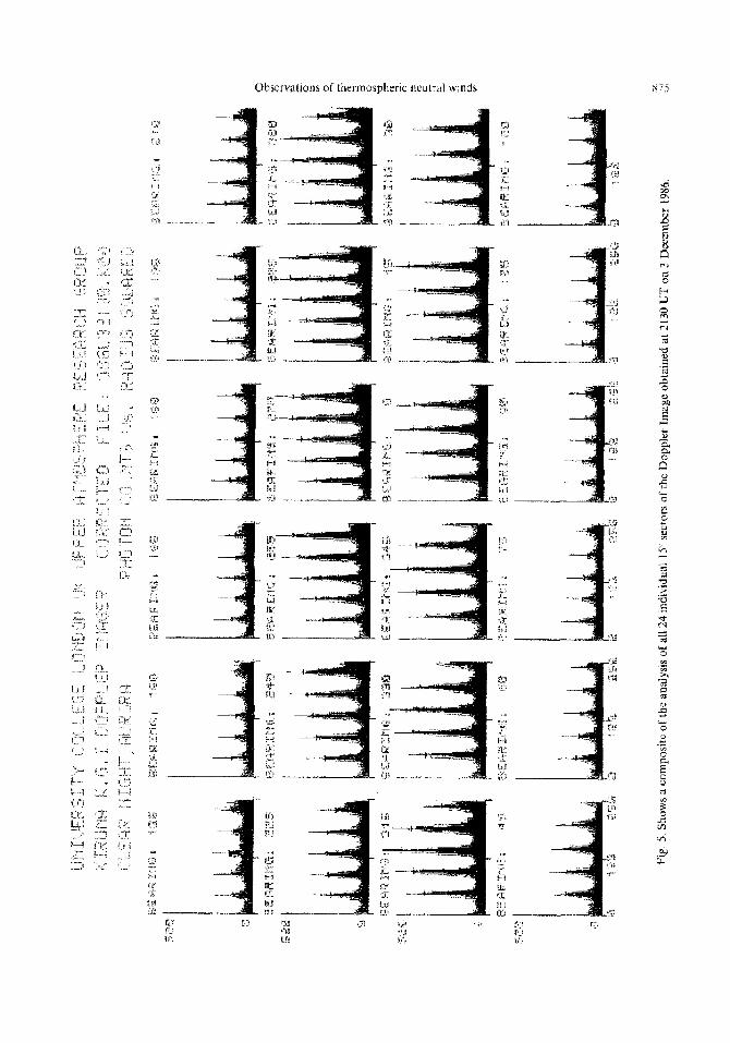
Figure 5 shows a composite of the analysis of all 24

individual 15” sectors of the single Doppler Image obtained at 2130 UT on 3 December 1986 (10 min integration). The data of the individual fringe peak locations, half-width and background, including errors are all stored in a designated data file for subsequent analysis.

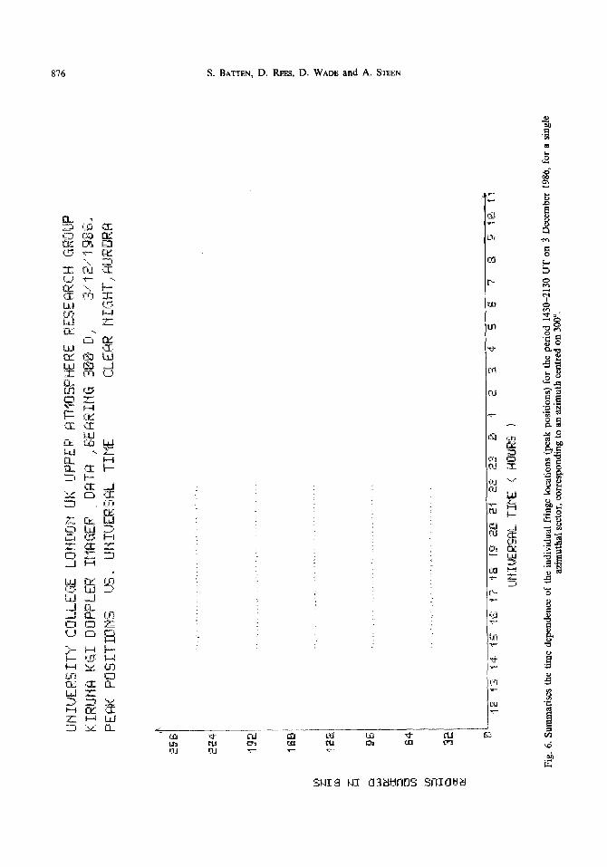
Figure 6 summarises the time dependence of the individual fringe locations (peak positions) for the period 143&2130 UT on 3 December for a single azimuthal sector, corresponding to an azimuth centred on 300”. The figure emphasises that the individual Doppler Shifts are, in fact very small, compared with a free spectral range (inter-order fringe separation).

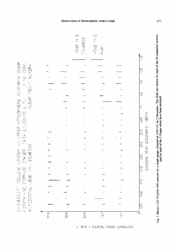
Figure 7 shows a full Doppler shift analysis for a single image. The shifts for each azimuthal sector and for each of the 5 fringes which have been analysed, are relative to the ‘zero velocity’ fringe position. This has been determined for the instrument via full-field spectral calibrations and via a long sequence of images obtained during cloudy periods and when the ‘standard’ UCL FPI at KG1 was indicating low Doppler shifts (a combination of low winds and/or cloudy sky conditions).

Primarily blue line-of-sight Doppler shifts are observed around 20&300 azimuth (i.e. wind directed toward, from the west), while primarily red Doppler shifts are observed at azimuthal angles of 45”-120” (i.e. wind directed away, toward the east). The line- of-sight component generally increases going outward from the first fringe. This is precisely what would be expected if the wind field were fairly uniform over the entire field of view so that the line-of-sight component would increase with the zenith distance (which increases from inner to outer fringe). Around a single fringe, the Doppler shift would display a purely sinusoidal variation. The peak Doppler shifts correspond to about 200 rns- ’ line-of-sight wind, some 250 ms- ’ at the zenith distance if this is a purely horizontal wind. Following the azimuthal variation of any single fringe there are slight departures from a purely sinusoidal variation with azimuth angle. Similarly, the Doppler shift variations from fringe to fringe are not entirely

consistent with a uniform wind field over the entire field of view. It is the objective of the subsequent stages of data analysis to determine which of the azimuthal and zenith distance variations may reflect real thermospheric wind variations, and which may be artifacts due to photon statistics, or other errors.

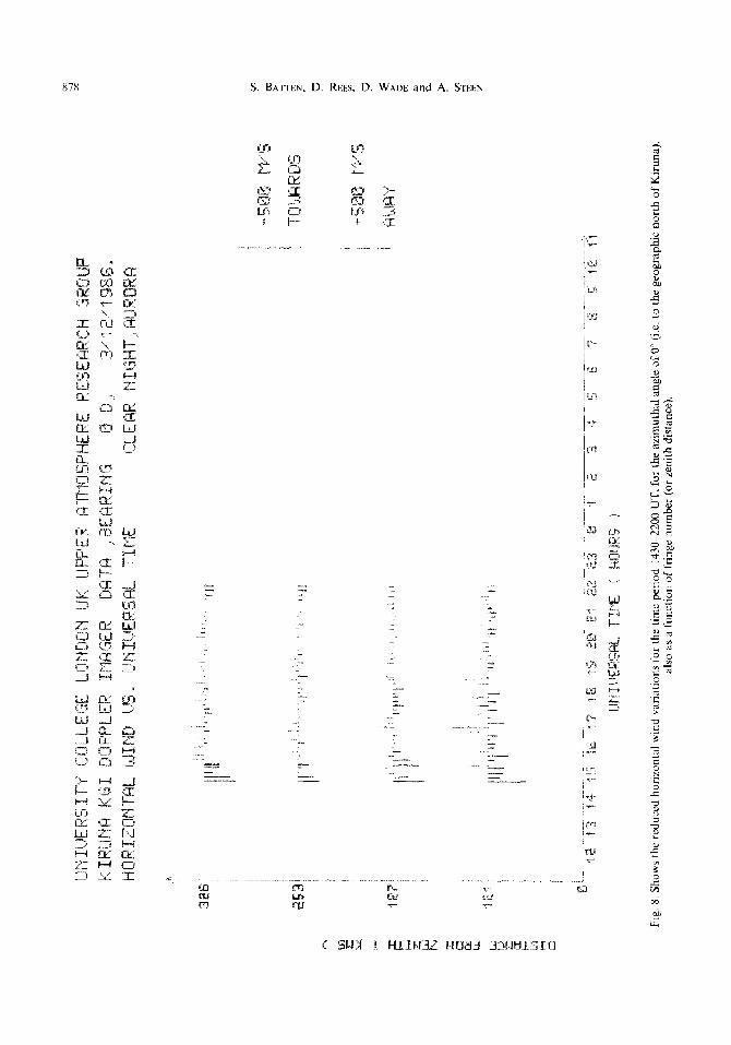
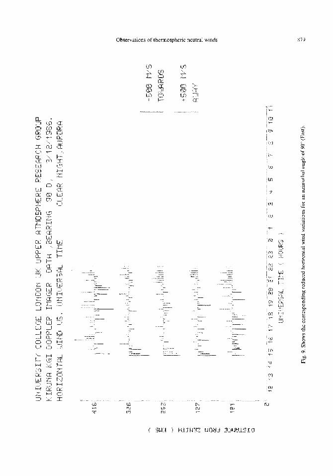
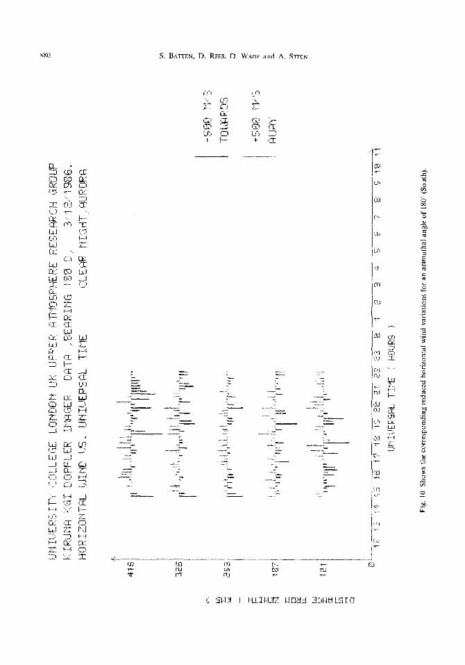
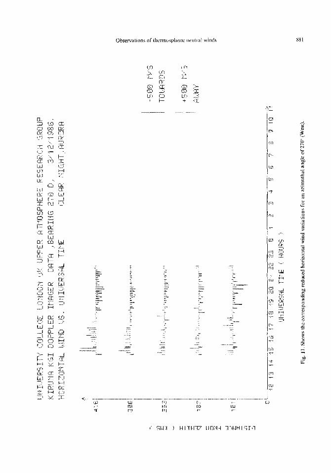
In Fig. 8. the Doppler shifts obtained in the 0” (north) azimuthal sector over the observing period have been corrected to horizontal wind components. Figures 9, 10 and 11 show the corresponding reduced horizontal wind variations for 90” (east), 180” (south) and 270” (west) azimuthal angles, respectively. Within


each of Figs. 8-l 1 the patterns of toward and away horizontal winds are consistent as a function of zenith distance or fringe number (also hoizontal range from Kiruna). This is in addition to the consistency observed with azimuthal angle within each fringe pattern (or Doppler image). Figures 8-l 1 also show that there are persistent patterns of the horizontal winds within each azimuthal sector.

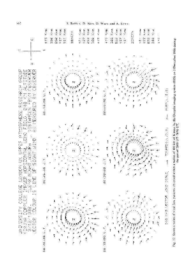
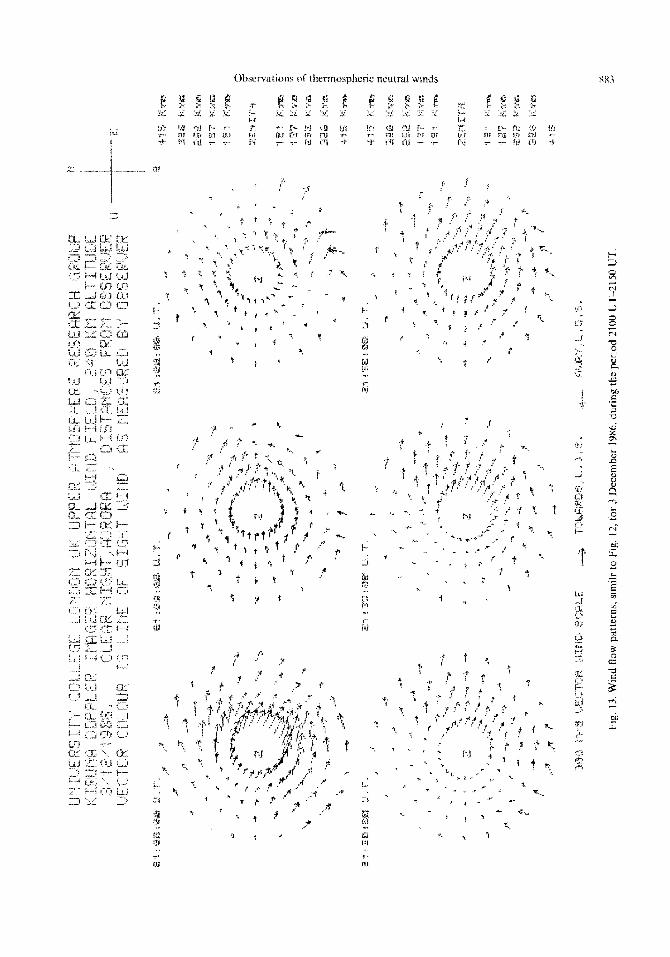
A series of reduced Doppler wind patterns obtained between 2000 UT and 2150 UT on 3 December 1986 are displayed in Figs. 12 and 13. These were obtained at 10 min intervals around magnetic midnight. The line-of-sight components, reduced to horizontal winds were displayed in Figs. 8-l 1 for individual ‘view directions’. In producing the plots shown in Figs. 12 and 13, continuity considerations have been used in cal- culating the unmeasured tangential wind component at each individual location in azimuth and zenith distance, as described previously. These individual observations have been filtered when applying a maximum entropy constraint. The deduced horizontal wind patterns reflect our best judgment of the maximum amount of valid spatial information available within each Doppler image, consistent with the quality of the available data. The data quality varies within each image, and from image to image, mainly as a function of aurora1 01630 nm intensity.

The mean winds, throughout the region of approximately 400 km radius explored by the DIS around Kiruna between 2000 and 2150 UT, are eastward directed. This is in contrast to the mainly westward winds observed earlier in the night, up to 1900 UT, as shown by the Doppler shifts in Figs. 8-l 1. Some quite dramatic wind changes occur during the two hour period displayed. The eastward and south- eastward winds, particularly to the north-west of Kiruna, intensify sharply around 2040 and 2100 UT. To the south and south-east of Kiruna there appears to be a relatively persistent reversal of the meridional component compared with the meridional component over Kiruna and to the north. In the general sense, strong flows away from Kiruna to the north-east and south-east appear to compensate for the inflow from the north-west and west. Unexpectedly, there seem to be intervals of the order of 20-40 min where the overall flow pattern moderates quite significantly. For example, after 2110 UT, the overall eastward flow drops from 300 ms- ’ to 200 ms- ‘, and subsequently the maximum winds appear to be around the latter value, although there are considerable fluctuations about the mean flow.

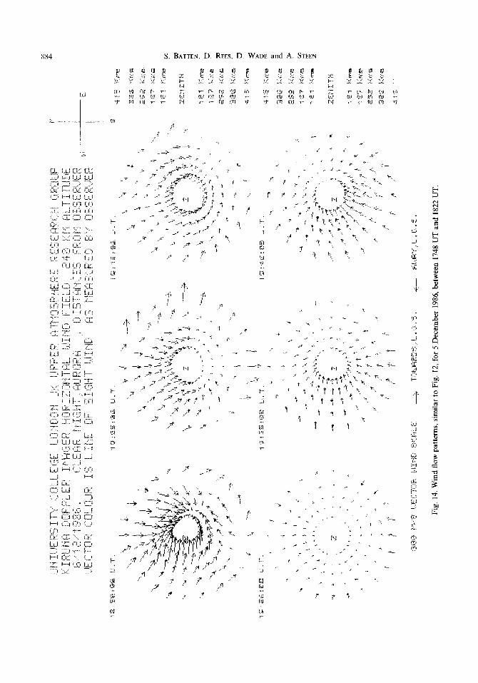
In Fig. 14, data obtained during the night of 5 December are shown. In this case, the 5 snapshots reflect rather disturbed conditions prior to geo-

magnetic midnight, in the period 1740-1820 UT. The mean flow velocity is between 300 and 400 ms- ‘, a relatively typical value for the pre-midnight period at the time of a significant positive excursion of the X magnetic component (indicating northward electric fields and strong westward drifting ion flow). The flow patterns present a picture of considerable complexity within the overall westward to south-westward flow. There is a hint in the flow images that a series of waves of higher velocities are propagating through the field of view. At the relatively high wind speeds, these waves would not be fully resolved at the 10 min intervals (and integration times) used to collect these data.

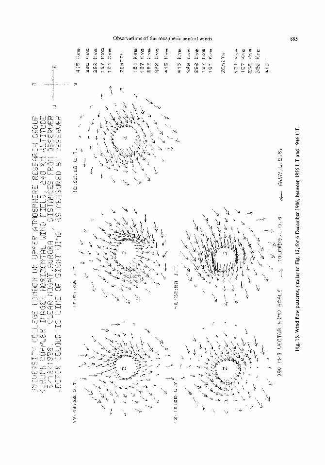
Figure 15 shows a comparable presentation of wind data obtained on 6 December 1986. This time, the flows are distinctly ‘post magnetic midnight’, that is primarily eastward. At the start of the data period (1850 UT), there is a strong wind surge from the north-west, with peak winds of up to 450 mss ‘. By 1926 UT, the entire wind pattern has become quiet, with maximum winds of around 200 ms- ‘. Later, the wind pattern shows a systematic north-eastward flow, which is a relatively unusual direction, although the maximum wind speeds barely reach 200-250 mss ‘. In most of the wind patterns there is again considerable complexity, which can be contrasted with the smooth transitions predicted by numerical simulations, which depend on averaged patterns of electric fields and precipitation.

8. DISCUSSION

None of the wind velocities observed during the periods reported here were particularly high, with maximum wind speeds reaching around 30@450 ms- ‘, typically 30-50% ofmaximum values observed during very disturbed nights (Rnns et al., 1985). However, the wind flows and structures changes are interesting, since they show spatial and temporal scales which have been below the resolution limits of previous instruments. Most of the smaller-scale wind features would not have been clearly registered and resolved by any of Fabry-Perot interferometers we have previously deployed at Kiruna, which scan sequentially in azimuth in the cardinal directions (N, NW, W, S, zenith, E, NE, N and ‘Cal’).

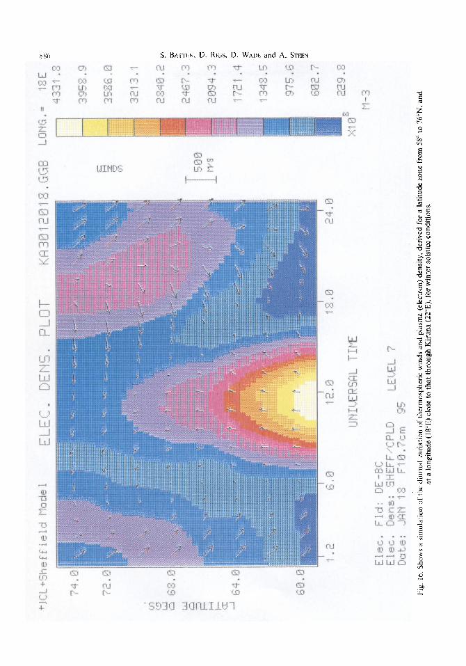
Figure 16 shows the upper thermospheric wind and ionospheric plasma density distribution (280 km), taken from a coupled global thermosphere/high latitude ionosphere simulation (FULLER-R• WELL and REES, 1980; FULLER-R• WELL et al., 1987), for winter solstice conditions. The model data have been extracted, as a function of universal time, for 18”E

870 S. BATTEN, D. REELS, D. WADE and A. STEEN

longitude, close to that of Kiruna (22”E). The simu- lated solar activity conditions are rather higher than those appropriate to December 1986, but the geomagnetic activity variations are rather similar (Kp N 3). At the latitude of Kiruna (67”N), the simulation predicts predominantly sunward and westward winds in the afternoon period, with the strongest winds to the north of Kiruna. The strongest winds occur immediately under the aurora1 oval and ion drag is the predominant reason for the strong sunward wind flow (REES et al., 1985). At lower latitudes than Kiruna, both in the early afternoon hours and the early morning hours, the wind flow is anti-sunward, the normal global low and mid-latitude flow away from the sub-solar point. Following the apparent motion of the aurora1 oval, the strongest winds migrate equatorward during the afternoon hours. There is an abrupt change in the wind pattern close to 210&2200 UT (magnetic midnight, or the Harang discontinuity), when the winds change rapidly from sunward (westward) to southward or south-eastward (REES et al., 1987) when Kiruna comes under the influence of strong (200-400 rns ‘) anti-sunward winds, following trajectories which have passed over the geomagnetic polar cap. The origin of these winds is not as simple or as local as is (predominantly) the case of the winds of the evening aurora1 oval, but rather reflects a complex interplay of solar forcing on the dayside flow continuity over the entire aurora1 oval and polar cap regions and some further acceleration by ion drag within the polar cap.

The simulation shown in Fig. 16 (generated for a situation when IMF By was negative) predicts a change from westward winds before 1800 UT, to south- eastward winds after 2000 UT. This situation (with UT the only variable) is relatively similar to the mean wind flows shown for 2030 UT to 2130 in Figs. 12- 15. It is also consistent with the wind values shown for individual azimuthal sectors in Figs. 8-l 1. Many small scale wind features, of relatively short duration (2&40 min) are observed in the DIS data which have no counterpart in the simulation, which contains no strictly time dependent terms, other than the variations resulting from the progression of universal time. In the context of this present paper, it is not practical to interpret these smaller scale features in detail. Further joint studies, using data obtained when the EISCAT and other radars were able to map ion flows and plasma concentrations, or when spaceborne aurora1 imagers, such as those on DE-2 and the VIKING spacecraft, were providing data will be used for detailed studies of the interplay of precipitation, heating and ion drag on the evolution of the thermospheric winds during extended observing periods.

The smallest scale wind field structures in the data presented here, which meet reasonable confidence cri- teria (+/-20 ms-‘), are of the order of 100-200 km in size. These wind field structures evolve quite rapidly. They are resolved by the 10 min integration time and interval between images, and are generally coherent between successive images and adjacent regions within particular images. In the future, particularly during periods of disturbed geomagnetic and intense aurora1 activity, shorter (2-5 min) integration periods will be used. This will reduce the spatial and temporal smearing of rapidly evolving and high velocity wind structures. When maximum winds of IO@ 200 ms- ’ occur, the wind field smearing is not a major limitation (60 km at 100 mss’ in 600 s integration period). However, particularly near solar maximum, winds of 50&800 ms- ’ are observed at Kiruna during major disturbances and parcels of air at such speeds would travel 30&500 km during the present 10 min integration period. Such a horizontal transport would completely smear any small (5&100 km) features of the horizontal wind patterns.

During the period for which wind data from the DIS are reported here, some quite interesting features were observed. Several of the wind changes imply sudden wind accelerations of l&20 min duration over regions of the order of 100 km diameter. Figs. 12 and 13, for example, show repetitive pulses of increased eastward/south-eastward winds which occurred at intervals of the order of 40 min between 2000 and 2200 UT, during a period of moderately disturbed aurora1 and geomagnetic conditions. In these two figs. there is also an indication of a possible ‘back- wash’ from regions south and east of that under observation (centred on Kiruna), in the intervening periods between the times of highest general eastward wind speeds. As usual, when an interesting phenomena occurs toward or at the edge of the field of view, the spatial coverage limitations of the DIS are already exposed : a further extension of the field of view would be even more interesting.

Figure 14 (5 December) shows the highest wind speeds of any of the periods discussed here and, perhaps not surprisingly, the wind field is also rather choatic, with rapid wind changes.

Distinct wind flow reversals, compared to the mean observed wind flow are shown, for example, the reversal of the meridional wind component between 1858 and 1946 UT on 6 December (Fig. 15). Such wind flow features and variations are probably endemic during periods of moderate to intense aurora1 and geomagnetic activity in the vicinity of the aurora1 oval. The DIS is now capable of mapping such features, although in the immediate future the somewhat

Observations of lhermospheric neutral winds

J _____-.-- __-_

_ _ e...,.. __ --.. _-------

I __.“_ -.----

I

x72 S. BATTEN, D. REES, D. WAIIE and A. STEEN

Observations of thermospheric neutral winds x73

x74 S. BAT-KS. ID. RYES, D. Wnm and A. STEEN

Obscrvakms of thermospheric neutral wmds 57j

X76 S. BATTEN, D. REES, D. WADE and A. STEEN

Observations of thermospheric neutral winds

-

-

-

-

.-

-

-

-. _:.L A_, c

-c

x7x S. BATTEN, D. REES, D. WADE and A. STEEN

_

-- x.. . . 1

-._ ; 2”. z.

- ~-- .- _-. .- . ,.“. - -_

: .._-- -- -..+ =--. --

..^ -_ --L-.

_~ 2--

_I


Al__

“.__ . ..-- . ..I= .-I-- ^-.._

-‘- . .

-

.,:

_~ “.___ .-._- _.,_... ..::

1.

_.

- .

“,.

_ -.__^ “- z= “.~__~_

- .._..- ---- _-

,A

.L-.__

-,

_.____ - -y__ ._ - -

S. BATTEN, D. REES, D. WADE and A. STEEN

-_ -...z

__.___a

=

___

_A

+-

_-_

.,II-

I.,-,.-

I

L

w

-- --

_I

-1 -7

-_ .

-ZZ _.I_

z

z- _“. .

‘1

-- --

-:r, -a

.._-

;:

.-I

_-

s “,__?..

---

_,

“_..“x

A -

-- “L _

“... -


. -.” -- -- z--

_ - - I

,_

1_. -

_..

i-

:: . L

..l__-..

,-.

-._.._--_ -,,-.1___1

A-.

. ._

!t.:

s-- ~-. ----IL-- _i -

j

‘3

I ii 4 . , ,?

Observations of thermosphetic neutral winds xx3

; t

S, BATTEN, D. REES, D. WADE and A. STEEN

<_. C-

? _-

_._ -4

bX6 S. BATTEN, D. REES, D. Wmt, and A. STEEN


onerous data analysis process will limit its use to ‘cam- Acknowledgemeru-The Doppler imaging system was orig- paign’ periods during disturbed nights, to experiments inally conceived, designed and built with considerable assist-

in conjunction with the EISCAT Radar system, and ante from ALAN GREENAWAY, MARTYN WELLS, IAN

to observing programmes coordinated with spacecraft MCWHIRTEX, KEITH SMITH and JIM PERCIVAL. The work has been supported by grants from the Science and Engineering

overpasses or joint global observing periods: Research Council.

BRACEWELL R. M

COOPER V. G. FULLER-R• WELL T. J. and REES D. FULLER-R• WELL T. J., m D., QLJEGAN S.,

MOFFE~ R. J. and BAILEY G. J. HAYS P. B. and ROBLE R. G. HAYS P. B., KILLEEN T. L. and KENNEDY B. C. HAYS P. B., KILLEEN T. L., SPENCER N. W.,

WHARTON L. E., ROBLE R. G., EMERY B. A., FULLER-R• WELL T. J., REES D., FRANK L. A. and CRAVEN J. D.

HEZRNANDEZ G. HERNANDEZ G.

KIELKOPF J. F. KILLEEN T. L., HAYS P. B., SPENCER N. W.

and WHARTON L. E. KILLEEN T. L., ROBLE R. G., SMITH R. W.,

SPENCER N. W.. MERIWETHER J. W.. Rnns D.. HERNANDEZ G.; HAYS P. B., COGGED L. L., ’ SIPLER D. P., BIONDI M. A. and TEPLEY C. A.

KILLEEN T. L., KENNEDY B. C., HAYS P. B., SYMANOW D. A. and CECKOWSKI D. H.

K~~PMANS L. H.

MCWHIRTER I., REES D. and GREENAWAY A. H. REES D., MCWHIIUER I., ROLJNCE P. A.

and BARLOW F. E. REES D., ROUNCE P. A., CHARLETON P.,

FULLER-R• ~ELL T. J., MCWHIRTER I. and SMITH K.

REES D., FULLER-R• WELL T. J., GORDON R., KILLEEN T. L., HAYS P. B., WHARTON L. E. and SPENCER N. W.

REES D. and GREENAWAY A. H. REES D., GREENAWAY A. H., GORDON R.,

MCWHIRTER I., CHARLETON P. J. and STEEN A. REES D., FULLER-R• WELL T. J., GORDON R.,

SMITH M. F., KILLJZEN T. L., HAYS P. B., SPENCER N. W., WHARTON L. E. and MAYNARD N. C.

REES D.

REES D., FULLER-R• WFLL T. J., GORDON R., SMITH 1986 M. F., HEPPNEX J. P., MAYNARD N. C., SPENCER N. W.. WHARTON L. E.. HAYS P. B. and KILLEEN T. L.

REINS ‘D., LLOYD N. D, FULLER-R• ~ELL T. J. and STEEN A.

SHEPHERD G. G., LAKE C. W., MILLER J. R. and C~GGER L. L.

tEFERENCES

1965

1971 1980 1987

1971 1981 1984

The Fourier Transform and its Applications, pp. 9% 127. McGraw-Hill Inc. New York.

Appl. 0p1. 10, 525. J. afmos. Sci. 31,2545. J. geophys. Res. 92,7744.

Appl. Opt. 10, 193. Space Sci. Instrum. 5,395. J. geophys. Res. 89, 5547.

1978 1986

1979 1982

1986

Appl. Opt. 17,2967. Fabry-Perot Interferometers. Cambridge University

Press. J. Opt. Sot. Am. 69,482. Geophys. Res. Lett. 9, 957.

J. geophys. Res. 91, 1633.

1983

1974

1982 1981

1982

A@. Opt. 22,3503.

The Spectral Analysis of Time Series. Academic Press, New York.

J. Phys. E: Sci. Instrum. 15, 145. J. Phys. E: Sci. Instrum. 14, 229.

J. Geophys. 50,202.

1983 Planet. Space Sci. 31, 1299.

1983 1984

1985

Appl. Opt. 22,1078. Planet. Space Sci. 32, 273.

Planet. Space Sci. 33,425.

1986 Balloon borne wind observations of the stratosphere using a triple etalon Fabry-Perot interferometer. NASA proceedings of the Global Wind Conference, Deepak Limited (Ed.).

Planet. Space Sci. 34, 1.

1987 J. Geophys. 9, 197.

1965 Appl. Opt. 4, 267.


SHEPHERD G. G., DEANS A. J. and NEO Y. P. 1978 cm. J. Phys. 56,681. SIPLER D. P. and BIONDI M. A. 1978 Geophys. Res. L.ett. 5,373. SMITH R. W. and SWEENEY P. J. 1980 Nature 284,437. SPENCER N. W., WHARTON L. E., NIEMANN H. B., 1981 Space Sci. Instrum. 5,417.

HEDIN A. E., CARICNAN G. R. and MAURER J. C. WIENS R. H., GALJLT W. A., SHEPHERD G. G. 1987 Thermospheric wind measurements with a ground-based

and KOSTENIUK P. WAMDll. Presented at the CEDAR session, IAGA, Vancouver, August 1987.

observations of thermospheric neutral winds by the ucl doppler imaging system at kiruna in northern...

Documents