observation errors in early historical upperair … errors in early historical upper-air...

JOURNAL OF GEOPHYSICAL RESEARCH: ATMOSPHERES, VOL. 118, 12,012–12,028, doi:10.1002/2013JD020156, 2013

Observation errors in early historical upper-air observationsR. Wartenburger,1 S. Brönnimann,1 and A. Stickler1

Received 8 May 2013; revised 14 October 2013; accepted 16 October 2013; published 11 November 2013.

[1] Upper-air observations are a fundamental data source for global atmospheric dataproducts, but uncertainties, particularly in the early years, are not well known. Most ofthe early observations, which have now been digitized, are prone to a large variety ofundocumented uncertainties (errors) that need to be quantified, e.g., for their assimilationin reanalysis projects. We apply a novel approach to estimate errors in upper-airtemperature, geopotential height, and wind observations from the ComprehensiveHistorical Upper-Air Network for the time period from 1923 to 1966. We distinguishbetween random errors, biases, and a term that quantifies the representativity of theobservations. The method is based on a comparison of neighboring observations and ishence independent of metadata, making it applicable to a wide scope of observationaldata sets. The estimated mean random errors for all observations within the study periodare 1.5 K for air temperature, 1.3 hPa for pressure, 3.0 ms–1 for wind speed, and 21.4ı forwind direction. The estimates are compared to results of previous studies and analyzedwith respect to their spatial and temporal variability.

Citation: Wartenburger, R., S. Brönnimann, and A. Stickler (2013), Observation errors in early historical upper-air observations,J. Geophys. Res. Atmos., 118, 12,012–12,028, doi:10.1002/2013JD020156.

1. Introduction[2] Upper-air observations are crucial for the determina-

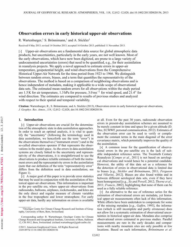
tion of the atmospheric state in data assimilation approaches.In order to reach an optimal analysis, it is vital to quan-tify the “uncertainty” (following the terminology used indata assimilation, we henceforth use the term “error”) inthe observations themselves (“instrument errors”) and in theso-called observation operator H that represents the obser-vations in the model space. As the errors in data assimilationsystems are closely linked to the uncertainty and represen-tativity of the observations, it is straightforward to use theobservations to produce reliable estimates of both the instru-ment errors and the representativity errors in the assimilation(note that our definition of the term “representativity error”differs from the definition used in data assimilation; seeFigure 1).

[3] A major goal of this paper is to provide error statisticsthat may be used in conjunction with the assimilation of his-torical upper-air observations. This information is importantin the pre–satellite era, where upper-air observations fromradiosondes, balloons, airplanes, rocketsondes, and kites arethe only direct and regular measure of climate variablesin the free troposphere and lower stratosphere. For earlyupper-air data, hardly any information on errors is available

1Oeschger Centre for Climate Change Research and Institute of Geog-raphy, University of Bern, Bern, Switzerland.

Corresponding author: R. Wartenburger, Oeschger Centre for ClimateChange Research and Geographical Institute, University of Bern, Hallerstr.12, CH-3012, Bern, Switzerland. ([email protected])

©2013. American Geophysical Union. All Rights Reserved.2169-897X/13/10.1002/2013JD020156

at all. Even for the past 30 years, radiosonde observationerrors in present-day assimilation schemes are assumed tobe merely constant in time and space for a given altitude (D.Dee, ECMWF, personal communication, 2012). Estimates ofthe observation error can be used to verify or comple-ment the constant terms in the main diagonal of the errorcovariance matrix, which potentially improves the quality ofthe assimilation.

[4] A common issue for the quantification of observa-tional errors in the pre–satellite era is the lack of suit-able independent reference series. The Twentieth CenturyReanalysis [Compo et al., 2011] is not based on aerologi-cal observations and would hence be a potential candidate.However, the utility of this data set as a reference forthe detection of errors in observational data is limited dueto biases [e.g., Stickler and Brönnimann, 2011; Fergusonand Villarini, 2012]. Biases are also found within and inbetween different aerological data sets, even if they havebeen homogenized [e.g., Xu and Powell, 2012; Thorne et al.,2011; Francis, 2002], highlighting that none of them can beused as a fully reliable reference.

[5] An alternative to the use of reference series for theestimation of observational errors are metadata, yet histor-ical upper-air measurements often lack of this information.While efforts have been undertaken to compensate for someof the missing metadata [e.g., Gaffen, 1993], the informa-tion (which is still incomplete and partly erroneous) doesnot allow for a systematic estimation of observational uncer-tainties in historical upper-air data. Metadata also compriseobservational errors estimated in previous studies. Parallelmeasurements are rare in the early decades and compar-isons with nearby mountain sites are only possible at fewlocations. Based on such information, Brönnimann et al.

12,012

source: https://doi.org/10.7892/boris.47221 | downloaded: 13.3.2017

WARTENBURGER ET AL.: ERRORS IN UPPER-AIR OBSERVATIONS

Figure 1. Comparison of terminologies for errors and uncertainties in observational data common inmeteorology and data assimilation. The terms used in this paper (leftmost column) refer to observation-based estimates (middle column) of errors relevant for data assimilation (rightmost column). Ox representsan observation, which deviates from the unknown true state of the atmosphere x by a bias term b and arandom error term e. The difference of x at two spatially distinct locations (subscripts c and r) is expressedas the representativity error of xc with respect to xr. The definition of the representativity error that isused in this paper differs from the one used in data assimilation, where it depends on the observationoperator H, and hence on the model grid. Random errors and representativity errors are estimated fromthe variance, biases are estimated from the mean. A mathematical definition of the error terms is providedin section 3.2.

[2011] estimated random errors of 0.9–1.2ıC and 1.35 hPa(standard deviations) for temperature and pressure measure-ments in German radiosonde data from the late 1930s. Firstcomprehensive in-flight experiments for the determinationof observational errors were performed in the 1950s [(OMI)Organisation Météorologique Internationale, 1951; (OMM)Organisation Météorologique Mondiale, 1952]. Jasperson[1982] experimentally estimated errors in wind speeds fora Doppler-based tracking system of pilot balloons. A num-ber of studies examined sonde drift errors in greater detail[e.g., McGrath et al., 2006; Seidel et al., 2011], while othersfocused on sonde-specific radiation errors [e.g., Brasefield,1948; Rossi, 1954]. Kitchen [1989] applied a comprehen-sive analysis of spatial and temporal representativity errorsfor UK Meteorological Office RS3 sondes. Although all ofthose studies provide valuable error statistics, they cannotbe used to infer error statistics for the full range of synoptichistorical upper-air observations.

[6] The issue of detecting and correcting systematic errorsin upper-air data is an active topic in climate research. Mostof the homogenization approaches are motivated by attemptsto produce homogenized observation series that are usefulfor the analysis of long-term trends. A variety of tech-niques for break detection and adjustment were investigated.Lanzante et al. [2003] developed an absolute homogeniza-tion method based on a semisubjective break detection.Free et al. [2005] investigated the first differences techniquefor the reduction of inhomogeneities. Thorne et al. [2005]developed a relative homogenization method based onneighbor composites. This method was expanded to a fullyautomated homogenization by McCarthy et al. [2008]. Other

approaches make use of innovation statistics of the EuropeanCentre for Medium Range Weather Forecast (ECWMF) 40Year Reanalysis (ERA-40) to homogenize radiosonde tem-peratures [Haimberger, 2007; Haimberger et al., 2008] andupper-air winds [Gruber and Haimberger, 2008]. Sherwood[2007] and Sherwood et al. [2008] address the homoge-nization of upper-air temperatures and wind shear of datasets that suffer from numerous gaps by applying a krigingmethod. Although all of these approaches succeed to pro-duce homogenized data sets, they all differ from the goalof this paper, which is to quantify the errors of individualupper-air observations.

[7] The error estimation approach presented in this paperdiffers from the techniques mentioned so far. It is basedon a direct comparison of observations from a candidateseries to neighboring reference series using aerologicaldata of the Comprehensive Historical Upper-Air Network(CHUAN) [Stickler et al., 2010]. By these means, weavoid the shortcomings of independent reference series ormetadata of questionable quality. Moreover, we are ableto estimate errors more comprehensively than previouslyby incorporating all observations that are available in thedata set.

[8] In the following section, we briefly describe the obser-vational data that the error estimation method is appliedto. Section 3 describes the error estimation method bothmathematically and technically and discusses sensitivities toparameter choices. In section 4, the method is tested againsta climatology and the estimated errors are discussed andcompared with independent estimates. The main findings aresummarized in the conclusions.

12,013


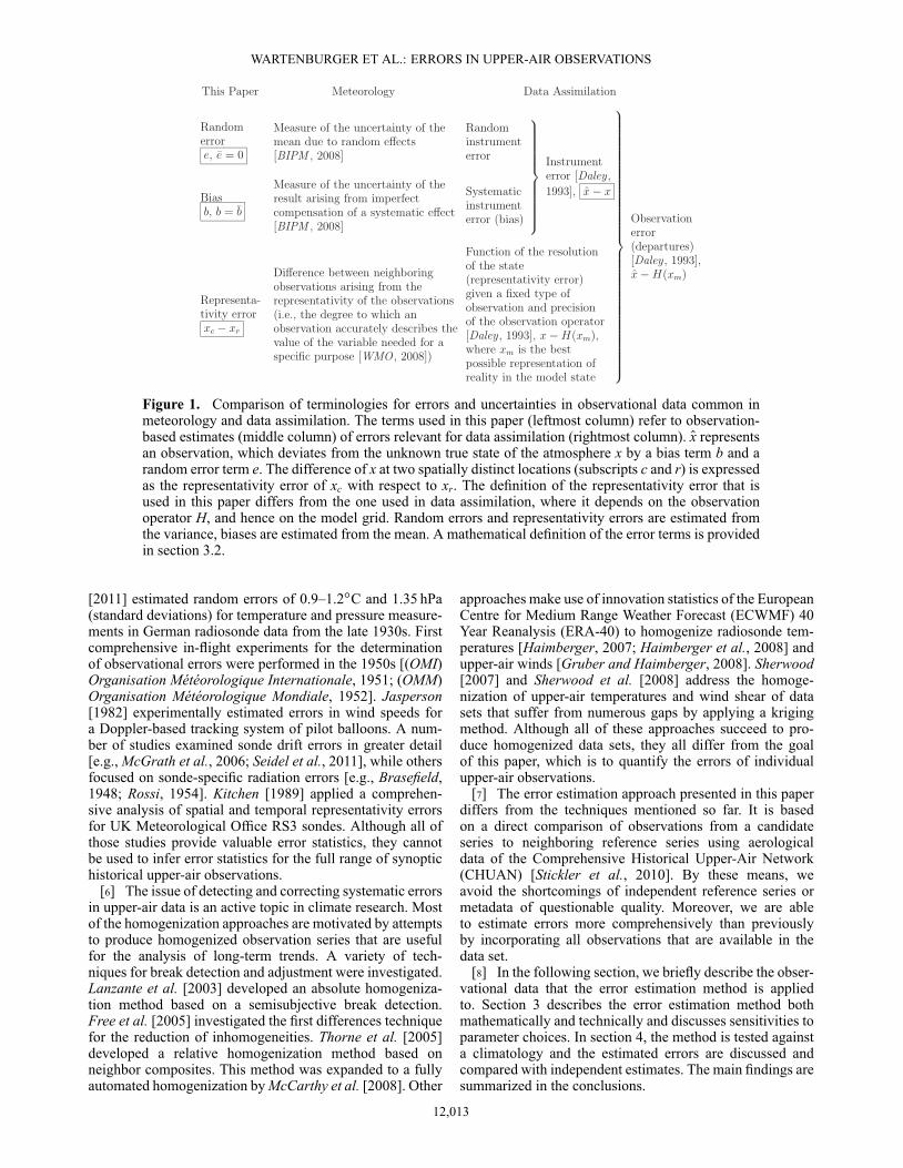
Figure 2. Locations and platform types of stations in operation during four distinct time spans asindicated on each map. Only stations with at least 30 observations are shown.

2. Observational Data[9] We analyze errors in the CHUAN data set, version

1.70 [Stickler et al., 2010]. The data set covers air tempera-ture, geopotential height, and wind observations from 4182stations in operation from close to the beginning of oper-ational upper-air observations in 1904 till the end of theInternational Geophysical Year (IGY) in 1958 (Figure 2).Continuous records were supplemented by observationsfrom the Integrated Global Radiosonde Archive (IGRA)[Durre et al., 2006] using RAdiosone OBservation COr-rection using REanalyses (RAOBCORE) 1.4 adjustments(which for the time period studied here is quasi-identical toRAOBCORE 1.5) [Haimberger et al., 2012]. To include thetransition time around the IGY, we analyze CHUAN obser-vations from 1923 (the earliest year for which error estimatesare available) till 1966. Each CHUAN record contains obser-vations from either aircraft, kites, pilot balloons, registeringballoons, or radiosondes. Due to different reporting prac-tices, observations are given on pressure levels or geometricaltitude levels.

[10] The adjusted version of CHUAN is used for theerror analysis (see Appendix A for technical details of theadjustment). For temperature and geopotential heights, sta-tistical break detection was performed, but adjustments werelimited to breaks that were confirmed by metadata (whichwas rare) or coincided with a change of source (mergingof different sources). Breaks were attributed to one of severalpredefined causes (such as a radiation error or a pres-sure offset) based on the shape of the vertical error profile[Brönnimann, 2003; Grant et al., 2009]. No additionalbreakpoints were used in order to circumvent the lack ofadequate metadata (e.g., unknown sonde types or on rareoccasions even unknown platform types). For winds, theobservations were compared to a reconstruction and manu-ally screened [Stickler et al., 2010, online supporting infor-mation]. Suspicious wind observations were flagged. Theresulting data set is considered to be free of large biases.It is deemed to be more appropriate for a detailed estima-tion of errors than the raw data, as the adjusted observations

resemble the characteristics of observations that would actu-ally be assimilated (raw observations are usually quality-screened prior to assimilation).

[11] Additional tests were performed on individual obser-vations of CHUAN to supplement the earlier quality checks,which were partly based on monthly means. The data set waschecked and corrected for inconsistencies in the file format.Range checks were applied to detect physically implausibleobservations, leading to an adjustment of the flags of sev-eral observations. Duplicate profiles containing observationson at least three altitude levels were removed (see remark inGrant et al. [2009]). For the estimation of biases, we makeuse of anomalies from a climatology based on 6-hourly fieldsof the ERA-Interim reanalysis [Dee et al., 2011] (technicaldetails are provided in Appendix B).

3. Errors in Aerological Observations3.1. Physical Error Sources

[12] Ideally, biases and random errors can be related totheir physical sources. Therefore, in order to better interpretthe errors, we briefly discuss the most important physicalerror sources. It is necessary to distinguish between thedifferent observation platforms and between the differentmeasurands and derived quantities (temperature T, pressurep, wind speed w, wind direction ‚, and geopotential heightZ). Errors (uncertainties) in these measurands are linked toindividual (partly overlapping) error sources.

[13] The magnitude of biases for both T and p is mainlycontrolled by the instrumentation type and by observa-tional practices common for an individual station network.For example, stations within the same network are usuallyequipped with the same sonde type, whose mean radiationerror differs from that common to other networks. Besidesthat, biases in T and p are commonly caused by a lag ofthe temperature sensor, by differences in the calibration, byerrors in the pressure sensor, or by deposition of ice or wateron the sensor [World Meteorological Organization (WMO),2008]. For w and ‚, biases are typically related to the type

12,014


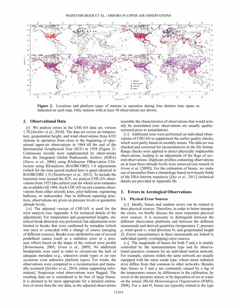
Figure 3. Schematic illustration of the assumed linearrelation between s2

Oxc–Oxr(y axis) and d2

c–r (x axis) for500 hPa temperatures measured at the candidate station3475 (Brunswick). The dashed line corresponds to the leastsquares fit, the dot-dashed lines indicate standard devia-tions of the residuals. The other lines illustrate the rela-tion between the squared station separation distance d2

c–r13(horizontal line) and the error terms used in equation (3)(variances; arrows). "13 is the residual of the thirteenth datapoint with respect to the least squares fit, and s2

xc–xr13is the

variance of the representativity error of the candidate seriesfor the distance d2

c–r13.

of balloon used, to the tracking device (optical theodolitesor radio-theodolites), or to the assumed ascent rate of theballoon [WMO, 2008]. Large biases in ‚ can be due toan incorrect calibration of the North direction (e.g., geo-magnetic North instead of geographic North) [Gruber andHaimberger, 2008].

[14] Some of the above-mentioned sources for system-atic errors do also cause random errors. Random errors inall variables can be caused by an imprecise assignment ofobservation times or by reading measured values from dis-crete scales [WMO, 2008]. For w and ‚, random errors arealso introduced by an imprecise tracking of the ascendingballoon and by the motion of the balloon relative to theatmosphere [WMO, 2008].

[15] The list of error sources presented here only has theintention to give a brief overview. Apart from the previouslycited literature, a more comprehensive listing of potentialerror sources in upper-air observations is provided, e.g., byGaffen [1994] or Häberli [2006].

3.2. Mathematical Error Description[16] An error is defined as the difference between an

observation Ox and the value of a measurand x (whichis unknown) [Bureau International des Poids et Mesures,2008]. It can be partitioned into a systematic part or biasb (time-invariant within the analyzed time window) and arandom part e, which is assumed to be symmetrically andunimodally distributed around a zero mean

Ox – x = b + e, with b = Nb and Ne = 0

where an overbar denotes an average over time. In manypractical applications, because x is unknown, we comparethe observation with a grid point value from another dataset or another observation. For the difference between twoobservations, we can write

Oxc – Oxr = (xc – xr) + (bc – br) + (ec – er) (1)

where (xc – xr) is termed representativity error. Apart fromrare exceptions (e.g., undetected copying of parts of theobservations from one station series to another one), it isreasonable to assume that ec and er are independent. Con-sequently, the variance (over time) of the difference can bewritten as follows:

s2Oxc–Oxr

= s2xc–xr

+ s2ec

+ s2er

(2)

To ensure that s2Oxc–Oxr

is a proper estimate for randomerrors, it is necessary to test if the distribution of Oxc –Oxr is normally distributed (which implies symmetry andunimodality). We applied the Anderson Darling Test ofGoodness of Fit [Anderson and Darling, 1954] and theJarque-Bera tests [Jarque and Bera, 1980]. The testssuggest that 82.0 % (82.2 %) of the temperature differ-ences, 81.6 % (81.4 %) of the geopotential height differ-ences, 73.7 % (78.2 %) of the wind speed differences, and88.0 % (76.0 %) of the wind direction differences are nor-mally distributed at a level of significance of ˛ = 10 %.These results suggest that our approach is suitable for theestimation of errors in T and Z, but less for the estimation oferrors in w and ‚. We still apply our approach to all vari-ables, but advise to be cautious in the interpretation of theestimated wind errors.

[17] The focus of this study is on random errors andrepresentativity errors. They are estimated for a given candi-date observation (subscript c) from a number of neighboring(or reference) observations (r1, : : : , rn). We further assume,for each pair, that the random error of both observationshas the same distribution (we assume that the geographicaldependency of random errors from neighboring stations isnegligible). Thus, we can write for the variances

s2Oxc–Oxr1

= s2xc–xr1

+ 2s2ec

...s2Oxc–Oxrn

= s2xc–xrn

+ 2s2ec

If we further assume that s2Oxc–Oxri

depends linearly on thesquared Euclidean distance d2

c–ribetween a candidate obser-

vation and a neighboring observation i, i = 1, : : : , n (ananalysis of scatterplots suggests that such a relation canindeed be postulated), a regression approach can be used toestimate s2

ecand s2

xc–xri

s2Oxc–Oxri

= c0 + c1 � d2c–ri

+ "i (3)

We interpret c0 as 2s2ec

, c1 as s2xc–xri� d2

c–ri, and "i as the uncer-

tainty inherent to the model. Equation (3) can be illustratedgeometrically (Figure 3). The uncertainty of the fit (whichis expressed as the standard deviation of the residuals ")is typical for candidate series with a moderate number ofreference series.

12,015


[18] Apart from random errors and representativity errors,we also estimate the bias b, which we further partition intoa network-wide bias bn and a station bias bs. For the time-average of equation (1) (Ne = 0), we get

Oxc – Oxr = (xc – xr) + (bnc – bnr ) + (bsc – bsr )

Within the same network (bnc = bnr ), we get

Oxc – Oxr = (Nxc – Nxr) + (bsc – bsr )bsc – bsr = NOxc – NOxr – (Nxc – Nxr)

Considering many reference stations (which are usuallylocated uniformly around the candidate station), we assumethat bsr is statistically independent and the average overall reference series (for a particular altitude level) is zero,[bsr ] = 0

[bsc – bsr ] = NOxc – Nxc – [NOxr – Nxr]bsc = NOxc – Nxc – [NOxr – Nxr]

For observations Oxnc and Oxnr , taken at all stations within twoadjacent networks, we thus get

hOxnc – Oxnr

i=�Nxnc – Nxnr

�+�bnc – bnr

�+�bsc – bsr

�

where we assume that the mean of all contributing individ-ual station biases relative to the respective network biases iszero, [bsc ] = 0 and [bsr ] = 0

�bnc – bnr

�=hNOxnc – NOxnr

i–�Nxnc – Nxnr

�

[19] The notation that is used in the rest of this paperrefers to the Euclidean distance between a candidate seriesand an arbitrary location as d, to the random error of acandidate series as se with s2

e = s2ec

, and to the respectiverepresentativity error as spd with s2

pd = s2xc–xri

/d2c–ri� d2 (i.e.,

s2xc–xri

normalized by distance; i = 1, : : : , n). We choose d2 =104 km2 (d = 100 km) to approximate the mean length scalesof the resolution of an ordinary model grid as used in mod-ern atmospheric reanalyses. To preserve the original units,we show the square root of abs(s2

e) and abs(s2pd). Values in

single square brackets ([]) correspond to spatial averages ona single altitude level, while errors in double square brackets([[]]) denote vertical averages.

3.3. Technical Error Description[20] For the implementation of the theory (previous

section) to real-world data (i.e., to sparse historical obser-vations), it is necessary to define a number of thresholdparameters. Obviously, the number of variance estimatess2Oxc–Oxri

, i = 1, : : : , n is limited by the number of referencestations n in the neighborhood of a candidate station. Wehence need to define an upper limit for the neighbor searchradius, max(d), and a lower limit for the number of referenceseries, min(rn). Individual reference series are only consid-ered, if at least 30 of their observations overlap in time withthose of the candidate series (a temporal overlap is con-strained by a time window �t centered at the observationtimes of Oxc). Multiple observation pairs within the same timewindow are allowed. To avoid large errors in wind direc-tions due to low wind speeds, wind directions are only used,if the corresponding wind speeds exceed 3 ms–1. For wind

directions, 360ı are subtracted from (added to) differencesthat are above (below) + (–) 180ı.

[21] The determined set of optimal threshold parametersis listed in Table A1. The parameters are defined by weigh-ing the number of candidate series cn (which equals the num-ber of error estimates) and the mean number of referenceseries [rn] against a set of statistical measures that define theoverall quality of each individual least squares model (seeequation (3); details are provided in Appendix C). In paral-lel to the parameter selection, we tested the sensitivity of theerror estimates with respect to various combinations of thethreshold parameters. It was found that the error estimatesare most sensitive to the choice of the neighbor search radius(max(d)), while the other threshold parameters only play amarginal role (see Appendix C). However, as the detectedoptimal values of max(d) are well in agreement with influ-ence radii determined from the average 0.5 decorrelationdistance (i.e., the average radius beyond which the spatialcorrelation drops below 0.5) for CHUAN observations in aprevious study by Griesser et al. [2010], we can adopt thesuggested values.

[22] Gross errors in the observations (e.g., large and sys-tematic processing or digitization errors) are likely to besmall in the analyzed (adjusted) version of CHUAN. How-ever, as the quality control and homogenization proceduresthat were previously applied to CHUAN were partly appliedon time scales greater than a month, some outliers are pos-sibly still present in the single ascent data. For this reason,we generate a subversion of the input data set for whichoutliers in the observation differences Oxc – Oxr are removedfor all combinations of Oxc and Oxr for which an error esti-mate could be computed. As a threshold for the detectionof outliers, we use the upper and lower fences fu and fl ofthe distributions of all observation differences determinedper measurand, level, and distance interval (intervals rangefrom (0, 100] km to ((max(d)–100), max(d)] km). The fencesfu and fl are a function of the upper and lower quartiles Q1and Q3: fu = Q3 + k � (Q3 – Q1), fl = Q1 – k � (Q3 – Q1)[Frigge et al., 1989]. As in the case of small sample sizes,the distribution of conventional quartile estimates may notbe strictly Gaussian, we use median-unbiased quartiles andthe standard value of 1.5 for the factor k [Hyndman and Fan,1996]. Individual differences Oxc – Oxr above (below) the upper(lower) thresholds are flagged for removal. The impact ofthe outlier treatment on the error estimates is briefly outlinedin Appendix C.

[23] Station biases bsc are determined for all candidateseries with at least min(rn) reference series. Network biasesare computed for all stations with a valid network identifierand min(rn) = 1 (stations using Vaisala sondes and stationswith unknown network identifier were considered to belongto the Vaisala network) [Grant et al., 2009]. The climatolog-ical difference Nxc – Nxr is computed using a climatology of theERA-Interim reanalysis (see Appendix B). We hereby makethe assumption that this climatology is a good estimate ofthe mean state of the atmosphere during the study period.

4. Results4.1. Test Against Climatology

[24] As the estimation of se and sp100 (i.e., spd for d =100 km) is based on statistical concepts, it is useful to

12,016


Figure 4. Profiles of mean random errors [se] (solid lines with filled symbols) and representativity errors[sp100] (dashed lines with open symbols) for (a) temperature, (b) wind direction, (c) geopotential height,and (d) wind speed estimated from the CHUAN observations (circles) and from the ERA-Interim clima-tology interpolated to the locations of the CHUAN stations (squares). Shaded bands indicate the standarddeviations of the random errors estimated from the climatology (light gray) and from CHUAN observa-tions (medium gray) for all stations; their overlap is printed in dark gray. Levels with less than 30 errorestimates were omitted.

validate the error estimation method. This can be achievedby applying the method to data sets with known errorcharacteristics (the parameters are the same as for the obser-vations, see Table A1). We make use of the interpolatedand smoothed ERA-Interim climatology (Appendix B). Thisdata set is preferred over a synthetic data set, as it containsmost of the statistical properties of real observational data,but no random errors (i.e., se = 0). If our regression approachfails to reproduce se = 0, its estimates (for a given variableand altitude level) are less accurate.

[25] The error profiles are shown in Figure 4. Not surpris-ingly, the observation-based estimates (both [se] and [sp100])are substantially different from the values that were derivedfrom the climatology. For Z, w, and T above 850 hPa, theestimated “random errors” of the climatology are approxi-mately symmetric to zero. For wind directions, the mean of[se] from the ERA-Interim climatology is shifted to the right,indicating that error estimates for this variable are ratherpessimistic. The amplification of [se] for ‚ and T near theearth surface can be explained by the biased sampling ofnear-surface observations in mountainous areas. However,substantial deviations from zero over the entire profile (‚)indicate that the relationship between s2

Oxc–Oxriand d2

c–riis not

strictly linear. Combining these results with the test of Oxc – Oxrfor normality (section 3.2), we can conclude that the errorestimates for both w and ‚ are potentially biased and haveto be interpreted with care. However, the test results indicatethat our method does succeed to produce reliable estimatesfor T and Z.

4.2. Biases[26] In the following, we discuss the station and network

biases, which were estimated for the entire study period.Besides our general interest in the results, the bias estimatesare useful to verify the bias adjustments that were previouslyapplied to CHUAN (Appendix A). In this respect, the mag-nitude of the biases indicates both the quality of the data setand the performance of the applied adjustments.

[27] The spatial distribution of station biases of T, w, and‚ on 500 hPa (5000 m) is shown in Figure 5. Only the North-ern Hemisphere is shown, as the number of estimated biasesin the Southern Hemisphere is too low (the same applies tose and spd). Based on the design of the applied method, biasestimates in regions of high station densities are assumedto be fully reliable, while they need to be interpreted withcare in regions where stations are not uniformly distributedin space (e.g., at continental margins). Temperature biaseshave no clear spatial patterns. Biases in winds are mostlyconstrained to observations within North America, while thedensity of overlapping observations in the other regions ismostly too low (note that the current version of CHUANdoes not include a sufficient number of wind observationsfrom the former Soviet Union). The range of station biases inwind speed and direction generally decreases with altitude,which likely indicates local differences in surface roughnessthat affect near-surface winds (not shown). Station biasesin w (Figure 5b) over the U.S. territory are marked by alatitudinal gradient from mostly negative biases at 30ıN tomore positive biases at around 40ıN. Similar features can

12,017


Figure 5. Spatial distribution of station biases (colored dots) for (a) 500 hPa temperatures, (b) 5000 mwind speeds, and (c) 5000 m wind directions. Small black crosses denote the location of stations for whicherrors were not determinable.

be found for ‚, where we find a prominent cluster of pos-itive biases at around 45ıN. The more isolated biases in‚ (which are constant throughout the entire profile) indi-cate systematic differences that might arise from the choiceof the wrong North direction. While these isolated biasesare clear indicators of systematic instrument or processingerrors in individual observation series, the spatially morecoherent biases could also be related to biases in the ERA-Interim reanalysis or to long-term changes in the patternsof the observed atmospheric fields. The confidence in these

interpretations could certainly be increased by consideringadditional data sets as a reference, which is certainly aninteresting perspective for future work.

[28] Figure A4 shows the profiles of network temperaturebiases for all combinations of neighboring station networks.The biases are generally low, but clearly depend on thechoice of the networks. The spread (˙1 standard deviation)among the differences of each observation pair is substan-tial, which underlines that the biases may be of differentmagnitude when considering shorter time spans or regional

Table 1. List of Mean Estimates (Variances), Mean Standard Errors of the Estimates (SE), Mean Coeffi-cients of Determination (R2, unitless), Mean Errors and Their Mean Horizontal Standard Deviations (sd)for 500 hPa (T, Z, p) and 5000 m (w, ‚)a

T (K2) Z (m2) w ((ms–1)2) ‚ ((deg)2)

Estimates [s2e ] 4.65 (2.76) 1299 (855) 17.8 (11.9) 1004 (189)

[s2p100] 0.0011 (0.0008) 0.63 (0.46) 0.0039 (0.0032) 0.29 (0.36)

Standard errors [SE(s2e )] 1.12 (0.66) 555 (351) 3.19 (1.75) 225 (157)

[SE(s2p100)] 0.0002 (0.0001) 0.090 (0.056) 0.0009 (0.0005) 0.051 (0.035)

Model fit [R2] 0.65 (0.74) 0.68 (0.72) 0.48 (0.65) 0.64 (0.84)

T (K) p (hPa) w (ms–1) ‚ (deg)

Mean errors [se] 1.46 (1.14) 1.58 (1.33) 2.90 (2.40) 21.64 (8.59)[sp100] 0.32 (0.28) 0.52 (0.44) 0.60 (0.56) 5.24 (5.91)

Horizontal sd [sd(se)] 0.45 (0.28) 0.74 (0.47) 0.77 (0.45) 6.05 (6.17)of mean errors [sd(sp100)] 0.08 (0.06) 0.16 (0.12) 0.18 (0.13) 1.40 (1.12)

aValues outside parentheses correspond to RAW and NF, values in parentheses correspond to RAW+OC and NF+OC.

12,018


Figure 6. Profiles of mean random errors [se] (solid lines with filled circles) and representativity errors[sp100] (dashed lines with open circles) for (a) temperature, (b) wind direction, (c) geopotential height, and(d) wind speed of the OC version. Open diamonds in Figure 6a correspond to observation errors assumedin the ERA-Interim reanalysis (see text). Shaded bands indicate the standard deviations of the randomerrors (medium gray) and representativity errors (light gray) for all stations; their overlap is printed indark gray. Levels with less than 30 error estimates were omitted.

subsets. Most of the temperature biases are in the range of˙1 K from the mean (and hence within the range of the sta-tion biases). However, for some combinations of networks,the biases clearly exceed the magnitude of the station biases.This indicates that, despite the previous adjustments appliedto CHUAN, systematic differences between the station net-works still exist in the data set. Biases on the 70 hPa and50 hPa levels are particularly large, which either indicatespersistent radiation errors in the Vaisala and U.S. networks,or an overcorrection of radiation errors in observations fromthe Soviet networks.

4.3. Random Errors and Representativity Errors[29] This section presents and discusses the final version

of the error estimates (T and Z: all available observations(RAW), w and ‚: all except flagged observations (NF); seeAppendix C). In cases where the focus is on the mean errorpatterns, we also present the outlier-corrected (OC) esti-mates. In the following, we first discuss the mean errorsand then analyze their spatial and temporal variability. If notdenoted explicitly, the presented estimates always refer tothe entire study period.4.3.1. Mean Errors

[30] Table 1 lists the estimated variances, the correspond-ing error estimates, their standard deviations (i.e., the spreadof all error estimates), and parameters that describe theuncertainty of the error estimates for the 500 hPa (5000 m)level. These levels were chosen, as they are often used torepresent the large-scale dynamic state of the atmosphereand are neither influenced by the planetary boundary layer

nor by tropospheric jets. The pressure errors are derived byconversion of the geopotential height errors using the 1976U.S. Standard Atmosphere [NOAA et al., 1976]. Both thestandard error of the estimates and the coefficient of deter-mination indicate that the error estimates of the OC versionare less noisy than the RAW (NF) estimates. In addition,[s2

p100] is less sensitive to the outlier removal than [s2e], which

underlines that the OC version can be used to analyze meanerror profiles. For all other analyses, we use RAW (NF), asit captures the full magnitude of [sd(se)] and [sd(sp100)].

[31] The mean profiles of the random and representa-tivity errors of the OC data allow for the identificationof factors that dominate the errors throughout time andspace (Figure6). For comparison, we also plotted the obser-vation errors for temperatures that are used in the ERA-Interim reanalysis. This error is assumed to be constant forall assimilated radiosonde observations on a given pres-sure level, whereas no distinction is made for differentsonde types or instrument designs (P. Poli, ECMWF, per-sonal communication, 2012). The representativity error ofthe data assimilation system (which is a component of theobservation error; cf. Figure 1) is arguably smaller thanthe estimated representativity errors, as the horizontal res-olution of ERA-Interim (T255) corresponds to grid celldistances that are (in average) smaller than the separationdistance d = 100 km. Throughout the troposphere, the esti-mated random errors are larger than the observation errors,while their vertical structure is well resembled. Given thatthe observation errors were specified at the time the ERA-Interim reanalysis was built, this result is in agreement

12,019


Figure 7. Spatial distribution of random errors (colored dots) and representativity errors (gray circles)for (a) 500 hPa T and (b) 500 hPa Z. Small black crosses denote the location of stations for which errorswere not determinable.

with the long-term increase in the accuracy of observationsover time (cf. Figure 10). On altitudes above 200 hPa, wefind a substantial disagreement of the errors that requiresfurther attention.

[32] The mean temperature representativity errors [sp100](Figure 6a) show maxima on the 850 hPa and 200 hPa lev-els. The 850 hPa peak is located within the global averageheight of the planetary boundary layer (500–2000 m, accord-ing to Seidel et al. [2010]), while the 200 hPa peak fallswithin the annual mean height of the midlatitude tropopause(� 150–250 hPa, according to Hoinka [1998]). Both peaksare most likely caused by height variations in these atmo-spheric features. In accordance to the high degree of spatialhomogeneity of the temperature fields in the upper tro-posphere and lower stratosphere, representativity errors atthese altitudes are low. The mean random errors are largestnear ground and show no peak on 850 hPa, which indicatethat they are mostly dependent on the observing system.They are, however, not fully independent of ambient weatherconditions. For instance, wrongly corrected instrument lagsmay lead to lower errors in areas where lapse rates arerather constant such as in the middle and upper troposphere.The spread in [se] indicates the heterogeneity of the con-tributing observations (note that the spread is larger in theRAW version).

[33] The mean profile of [sp100] for‚ (Figure 6b) is mainlycharacterized by a distinct decrease with height up to an alti-tude of� 23 km interrupted by a secondary maximum at analtitude of around 9–11 km (� 307–226 hPa), which is justbelow the annual mean height of the midlatitude tropopause.Despite the limited validity of the error estimation methodfor use with wind directions, the large magnitude of thevertical variation of [sp100] suggests a predominance of nat-ural, i.e., climatological factors. Random errors of ‚ arehigher near ground, where wind directions are more hetero-geneous due to different station altitudes and due to the influ-ence of surface roughness. The standard deviation over all

stations is low above 20 km and largest in the middle andupper troposphere.

[34] For geopotential height (Figure 6c), the strongincrease of the tropospheric representativity errors with alti-tude is dominated by an increase of the mean heights withaltitude, which cause an increase in spatial differences of Zmeasured within the radius max(d). Within the lower strato-sphere, the geopotential height gradients decrease again. Theincrease of [se] with altitude is due to the summation of theerrors in the pressure and temperature measurements dur-ing the radiosonde ascents. The lower value on the 70 hPalevel is related to the fact that this pressure level was mainlyreported in radiosonde ascents from the end of the studyperiod (which are characterized by smaller random errors).The spread of [se] is low compared to the heterogeneousdistribution of the respective representativity errors.

[35] The shape of the error profiles of w (Figure 6d) isdominated by the average altitude of the maximum windspeeds on � 12 km. The increase of [se] up to this altitudecan also be explained by the dependency of the angu-lar errors on the total distance between the theodolite andthe balloon. In the stratosphere, however, wind speeds aregenerally less strong and more homogeneous, causing a sub-stantial decrease of both random errors and representativityerrors. The magnitude of the spread is correlated to themagnitude of the mean errors.4.3.2. Spatiotemporal Error Structure

[36] The analysis of spatial error patterns is assisted bythe use of error maps. Figures 7 and 8 show the individ-ual random errors and representativity errors of all analyzedvariables on the 500 hPa (5000 m) level. Errors on this alti-tude are not substantially different from the neighboringlevels and are therefore considered to be characteristic forthe midtroposphere. What stands out for T and Z is a meanincrease of the representativity errors from the subtropicsto the subpolar region (see also Figure 9). This feature isin line with atmospheric circulation patterns that determine

12,020


Figure 8. Spatial distribution of random errors (colored dots) and representativity errors (gray circles)for (a) wind speed and (b) wind direction on 5000 m. There are no estimates for the former Soviet Union,as radiosonde winds in CHUAN V1.7 are too sparse, and the Soviet network in CHUAN V1.7 doesnot contain pilot balloons. Small black crosses denote the location of stations for which errors were notdeterminable.

the degree of spatiotemporal variability of the atmosphericfields (e.g., the position of the jet streams). No clear latitudi-nal trend in [sp100] is found for w and ‚. Random errors ofT and Z are dominated by above-average values over largeparts of the former Soviet Union, while they are generallylow over China, south-western Europe, the USA, and theCaribbean. This pattern is in agreement with the assump-tions of the method (se is the same for any reference seriesof a given candidate series), i.e., random errors are mostlythe same for neighboring stations, and differences mainlyoccur on longer spatial scales. This does also correspond tothe expectation that random errors mainly differ in betweendifferent station networks. For winds, a large number ofnon-U.S. stations cover only short and nonoverlapping timespans, impeding a global comparison. Random errors in w

(Figure 8a) tend to be very low in the (sub) tropical calmzones and increase toward the North. This is in contrast torandom errors in ‚ (Figure 8b), which are spatially moreheterogeneous and large in both the subtropical and the sub-polar regions. Considering the limited performance of theerror model for winds, these patterns should, however, notbe overinterpreted.

[37] In order to quantify the dependency of the error esti-mates on the station latitude, all estimates were zonallyaveraged over 10 degree bins (see Figure 9 for errors ingeopotential heights). Both [se] and [sp100] tend to increasewith (Northern Hemisphere) latitude. This is linked to thelocation of the dominating pressure cells and associated flowfeatures. The meridional gradient of atmospheric variabil-ity obviously explains the gradients of both errors, as an

Figure 9. Zonal 10 degree mean (a) random errors and (b) representativity errors of geopotential heighton selected pressure levels. Errors are plotted in the middle of the 10 degree bands.

12,021


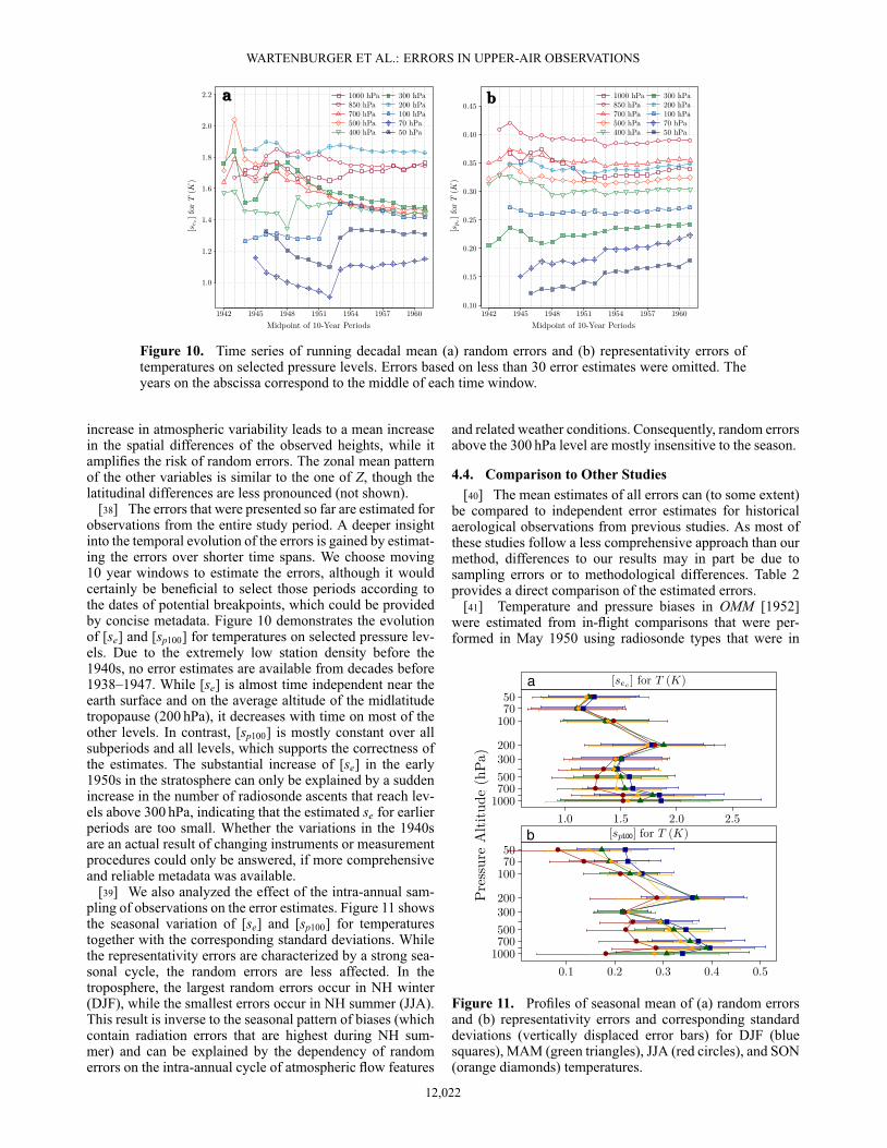
Figure 10. Time series of running decadal mean (a) random errors and (b) representativity errors oftemperatures on selected pressure levels. Errors based on less than 30 error estimates were omitted. Theyears on the abscissa correspond to the middle of each time window.

increase in atmospheric variability leads to a mean increasein the spatial differences of the observed heights, while itamplifies the risk of random errors. The zonal mean patternof the other variables is similar to the one of Z, though thelatitudinal differences are less pronounced (not shown).

[38] The errors that were presented so far are estimated forobservations from the entire study period. A deeper insightinto the temporal evolution of the errors is gained by estimat-ing the errors over shorter time spans. We choose moving10 year windows to estimate the errors, although it wouldcertainly be beneficial to select those periods according tothe dates of potential breakpoints, which could be providedby concise metadata. Figure 10 demonstrates the evolutionof [se] and [sp100] for temperatures on selected pressure lev-els. Due to the extremely low station density before the1940s, no error estimates are available from decades before1938–1947. While [se] is almost time independent near theearth surface and on the average altitude of the midlatitudetropopause (200 hPa), it decreases with time on most of theother levels. In contrast, [sp100] is mostly constant over allsubperiods and all levels, which supports the correctness ofthe estimates. The substantial increase of [se] in the early1950s in the stratosphere can only be explained by a suddenincrease in the number of radiosonde ascents that reach lev-els above 300 hPa, indicating that the estimated se for earlierperiods are too small. Whether the variations in the 1940sare an actual result of changing instruments or measurementprocedures could only be answered, if more comprehensiveand reliable metadata was available.

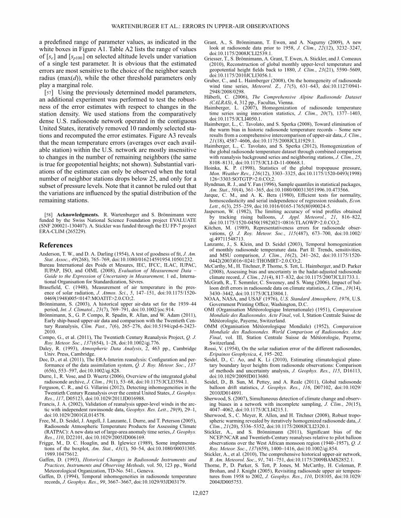
[39] We also analyzed the effect of the intra-annual sam-pling of observations on the error estimates. Figure 11 showsthe seasonal variation of [se] and [sp100] for temperaturestogether with the corresponding standard deviations. Whilethe representativity errors are characterized by a strong sea-sonal cycle, the random errors are less affected. In thetroposphere, the largest random errors occur in NH winter(DJF), while the smallest errors occur in NH summer (JJA).This result is inverse to the seasonal pattern of biases (whichcontain radiation errors that are highest during NH sum-mer) and can be explained by the dependency of randomerrors on the intra-annual cycle of atmospheric flow features

and related weather conditions. Consequently, random errorsabove the 300 hPa level are mostly insensitive to the season.

4.4. Comparison to Other Studies[40] The mean estimates of all errors can (to some extent)

be compared to independent error estimates for historicalaerological observations from previous studies. As most ofthese studies follow a less comprehensive approach than ourmethod, differences to our results may in part be due tosampling errors or to methodological differences. Table 2provides a direct comparison of the estimated errors.

[41] Temperature and pressure biases in OMM [1952]were estimated from in-flight comparisons that were per-formed in May 1950 using radiosonde types that were in

a

b

Figure 11. Profiles of seasonal mean of (a) random errorsand (b) representativity errors and corresponding standarddeviations (vertically displaced error bars) for DJF (bluesquares), MAM (green triangles), JJA (red circles), and SON(orange diamonds) temperatures.

12,022


Table 2. Error Estimates for (Historical) Aerological Observations for Given Pressure Levels (in hPa)a

Error Type and Vertical 900– 700– 500– 300–Source Variable Mean > 300 < 300 700 500 300 200 100 50 700 500 300 200

RAW [bnFI – bnr ] T (K) 0.13 0.18 0.23 0.15 0.17OMM [bnFI – bnr ] T (K) 0.79 0.60 0.60 0.75 1.05RAW [bnU.S. – bnr ] T (K) –0.22 0.10 –0.18 –0.50 –0.46OMM [bnU.S. – bnr ] T (K) –0.28 0.03 –0.10 –0.43 –0.58RAW [bnFI – bnr ] p (hPa) 0.49 0.59 0.70 0.63 0.41OMM [bnFI – bnr ] p (hPa) 4.4 1.5 1.5 5.5 6.5RAW [bnU.S. – bnr ] p (hPa) –0.04 0.48 0.44 0.11 –0.29OMM [bnU.S. – bnr ] p (hPa) –0.56 –2.30 –1.00 –0.30 0.80RAW [se] T (K) 1.50 1.58 1.41 1.49 1.46 1.49 1.41 1.27Brönn. [se] T (K) 0.9–1.2OMM [se] T (K) 0.77 1.25Zait. [se]b T (K) 0.50 0.70 0.90 0.65 0.40RAW [se] p (hPa) 1.26 1.57 0.77Brönn. [se] p (hPa) 1.35OMM [se] p (hPa) 5.75 8.33RAW [se] Z (m) 15.3 23.3 36.2 43.9 48.1Zait. [se]b Z (m) 5.0 9.5 26.0 38.0 48.0RAW [sp220] T (K) 0.8 0.7 0.5 0.8 0.6 0.4Kit. [sp220]b T (K) 11.5 16.7 24.3 23.4 16.6 15.5RAW [sp220] Z (m) 11.5 16.7 24.3 23.4 16.6 15.5Kit. [sp220]b Z (m) 26 37 55 50 40 38

aThe source of the data is indicated in the first column (OMM: [OMM (Organisation Météorologique Mondiale), 1952], Brönn.: Brönnimann et al.[2011], Zait.: Zaitseva [1993], Kit.: Kitchen [1989]). The subscript FI used for the network biases indicates the Finnish (Vaisala) network, the subscriptU.S. indicates the U.S. network, the subscript r indicates all other networks.

bError estimates are root-mean-square errors.

operation at that time. The biases were calculated as meandifferences from one sonde type with respect to all othersonde types for daytime and nighttime ascents below andabove the 300 hPa level. Biases in T for the U.S. sondetype are very close to our estimates, while the magnitudesof the other biases are clearly larger, possibly owing to theadjustments applied in CHUAN.

[42] The random errors of Brönnimann et al. [2011] arewithin the range of our estimates, while there is considerabledisagreement to the estimates of OMM [1952] (in particularfor pressure). The large magnitude of the pressure error esti-mates in the OMM intercomparison could be related to uniterrors. Zaitseva [1993] estimated random errors for temper-atures observed by historical sonde types used in the formerSoviet Union, which are considerably lower than our meanestimates. This difference is even more evident if we onlyconsider stations located within the former Soviet Union (cf.Figure 7).

[43] The representativity errors estimated by Kitchen[1989] for temperatures and geopotential heights are sub-stantially higher than our estimates of [sp220], while theirvertical structure is the same. The disagreement in the errormagnitudes can be explained by methodological differences(use of root mean squared differences instead of variances)and by the smaller number of soundings that the estimates ofKitchen [1989] are based on.

5. Conclusions[44] We developed an algorithm to systematically esti-

mate random errors and representativity errors of historicalupper-air wind, air temperature, and geopotential height(pressure) observations which we applied to observationsfrom the Comprehensive Historical Upper-Air Network(CHUAN) from 1904 till 1966 (earliest error estimates

possible from 1923). The error estimation method is basedon a comparison of neighbor series which neither requirescomprehensive metadata nor other independent data sets,but complements and confirms metadata-based analyses. Itcan readily be applied to other four-dimensional atmosphericobservational data sets.

[45] The estimated error magnitudes are in good agree-ment with some studies [e.g., Brönnimann et al., 2011], butnot others (which mainly estimated errors of lower magni-tude). The spatiotemporal dependence of the errors agreeswith theoretical expectations and also shows new features.Biases between station networks generally exceed biasesbetween neighboring station series, indicating the presenceof systematic differences between the networks. The esti-mated representativity errors show substantial latitudinaland seasonal variations for most of the variables. Their meanprofile is in agreement with the mean vertical structure of theatmosphere, while random errors are much less dependenton the atmospheric state. The random errors of the histor-ical observations are mostly larger than observation errorsassumed in a modern reanalysis product.

[46] Both the error estimation method and the estimatederror statistics can be used for data assimilation approaches.We provide information about the spatial and temporalrelations of random errors and representativity errors,which is important when attempting to assimilate historicalupper-air data. In additional analyses, spatial and tempo-ral error covariances could be computed from the estimatederrors, which are assumed to be zero in current assim-ilation schemes.

[47] Apart from its utility for the reanalysis community,the results can be applied to estimate errors in existing datasets by providing uncertainty measures for (historical) datasets that do not yet contain such information. Moreover, theerror estimates are suitable for a qualitative comparison to

12,023


Figure A1. Partial dendrogram of the individual decisionsI to VI (connecting lines) made for all parameters (grayboxes) and individual values that were tested (white boxes).Displayed are only the branches that were used for fur-ther analysis. The abbreviations in capital letters correspondto individual versions of the data sets: RAW (all availableCHUAN observations), NF (CHUAN observations exclud-ing flagged observations), and OC (CHUAN observationsexcluding outliers). Dashed lines correspond to decisionsrelated to wind observations only.

error estimates of reanalysis products (e.g., the ensemblespread or analysis departures of assimilated observations).Certainly, it would be rewarding for more expansive datavalidation efforts to develop a gridded data product from thecurrent point data (comparable to, e.g., Hadley Centre Atmo-spheric Temperature Data Set Version 2 (HadAT2); Thorneet al., 2005).

[48] The method that was presented in this paper isdesigned to be applied to other compilations of upper-airdata. A very promising candidate is the IGRA data set, whichcontains more extensive metadata that may aid to examinerandom errors and biases in greater detail. Another prospec-tive data sets are new compilations of historical upper-airobservations from the ongoing ERA-CLIM project. Thisdata set (which is planned to be included in the next versionof CHUAN (version 2.0)) will possibly allow for the estima-tion and analysis of observation and representativity errorsin regions that are currently blank.

Appendix A: CHUAN Adjustments[49] The adjusted versions of the CHUAN data set that

are used in this paper (C.DC for wind, C.DCR for tempera-ture, and geopotential height) were generated from the rawdata by applying a number of preprocessing steps. Suspi-cious observations of geopotential height and temperatureobservations were flagged according to their quality [Stickleret al., 2010, online supporting information]. Monthly meansof air temperature, geopotential height, wind direction, andwind speed were reconstructed using a variety of indepen-dent predictors [Brönnimann, 2003]. In order to test thegeopotential height and temperature observations for thepresence of artificial breakpoints, each of the station serieswas compared to reconstructed fields [Grant et al., 2009;Griesser et al., 2010]. Depending on the magnitude of theerrors, as well as on the skill of the statistical models,the station records were either (entirely or partly) rejected,adjusted, or accepted without adjustments. In addition to sta-tistical tests based on the comparison with a reconstruction

Figure A2. Profiles of mean random errors [se] (solidlines with filled symbols) and representativity errors [sp100](dashed lines with open symbols) for (a) wind direction and(b) wind speed of RAW (circles) and NF (squares). Shadedbands indicate the standard deviations of the random errorsestimated from RAW (medium gray) and NF (light gray) forall stations; their overlap is printed in dark gray. Levels withless than 30 error estimates were omitted.

12,024


Table A1. Optimal Values for the Threshold Parameters Used in the Error Estimation Method(Minimum Number of Reference Series min(rn), Maximum Separation Distance max(d), andTime Window Used to Treat Observations as Simultaneous �t) Determined by the Total Num-ber of Error Estimates cn, the Mean Number of Reference Series [rn], the Mean Coefficient ofDetermination [[R2]], the Mean Coefficient of Variation [[cv]], and the Mean p Value of the FTest of Goodness of Fit [[pF]]a

Variable Parameter cn " [rn] " [[R2]] " [[cv]] # [[pF]] # Decision

T min(rn) 4 10 7 4 10 6Z min(rn) 4 10 6 4 10 6w min(rn) 4 10 9 4 10 6‚ min(rn) 4 10 10 4 10 6T max(d) (km) 2000 2000 1500 1000 2000 1500Z max(d) (km) 2000 2000 1600 1000 2000 1500w max(d) (km) 2000 2000 1100 700 1800 1200‚ max(d) (km) 2000 2000 1300 800 1900 1300T �t (h) 6 6 0 1 0 3Z �t (h) 6 6 0 6 0 4w �t (h) 4 6 2 6 6 5‚ �t (h) 1 1 1 6 1 2

aThe range of tested values is indicated in Figure A1. Arrows indicate whether the threshold parameterswere selected for the lowest (arrow pointing downward) or highest (arrow pointing upward) values thatwere tested. The final selection of a threshold parameter (rightmost column) corresponds to the average ofcolumns 3–7 rounded to the next tested value. Values printed in italics were not considered, while valuesprinted in bold were weighted times 4.

similar to Griesser et al. [2010], wind observations were alsoevaluated by means of a detailed visual inspection [Stickleret al., 2010]. The applied adjustments for air temperature andgeopotential height compensate for radiation and lag errors(i.e., an error due to the lagged response time of the sen-sor), erroneous units, pressure errors, as well as for constanttemperature offsets [Grant et al., 2009; Brönnimann, 2003].If possible, physics-based adjustments were applied to theradiosonde observations to account for sonde-specific errorcharacteristics [Stickler et al., 2010].

Appendix B: ERA-Interim Climatology[50] We used 6-hourly ERA-Interim fields to generate

a climatology of the same spatiotemporal resolution that

is based on the reference period 1981–2010. The u andv wind fields were converted to wind speed and directionand linearly interpolated to the height of the geometric alti-tude levels used in CHUAN by using the gravity-correctedgeopotential height fields as a reference. After this step,all fields were spatially (bilinearly) interpolated to the geo-graphical locations of the CHUAN stations. Then, the inter-polated climatologies for each of the main synoptic hours(00, 06, 12, and 18 UTC) were filtered using a circular31 day running mean filter with equal weighting. For eachobservation series, the smoothed climatologies were theninterpolated to the respective ascent times by using naturalsplines to simulate the daily cycle. Anomalies were gener-ated by subtracting the difference between the observationsand the climatology.

Table A2. Range of [se] and [sp100] for All Variables on Selected Pressure (Geometric Altitude) LevelsUnder Variation of the Threshold Parameters min(rn), max(d), and �t

min(rn) 2 [4, : : : , 10] max(d) 2 [500, : : : , 2000] km �t 2 [0, : : : , 6] h[se] [sp100] [se] [sp100] [se] [sp100]

T850 (K) [1.43, 1.46] [0.48, 0.49] [1.18, 2.08] [0.32, 0.66] [1.77, 1.78] [0.39, 0.39]T500 (K) [1.18, 1.25] [0.38, 0.39] [0.93, 1.75] [0.26, 0.47] [1.46, 1.48] [0.32, 0.32]T300 (K) [1.25, 1.34] [0.30, 0.31] [0.96, 1.68] [0.19, 0.40] [1.49, 1.51] [0.24, 0.24]T100 (K) [1.28, 1.32] [0.30, 0.31] [1.10, 1.58] [0.24, 0.38] [1.41, 1.42] [0.27, 0.28]T50 (K) [1.12, 1.24] [0.18, 0.23] [1.00, 1.38] [0.18, 0.24] [1.25, 1.29] [0.20, 0.20]Z850 (m) [10.4, 11.1] [4.8, 0.50] [8.7, 17.9] [3.8, 5.3] [13.7, 14.2] [4.4, 4.4]Z500 (m) [17.9, 18.9] [8.4, 8.8] [15.4, 31.3] [6.6, 9.3] [23.9, 24.6] [7.7, 7.7]Z300 (m) [28.8, 29.8] [12.5, 12.8] [23.2, 48.0] [9.5, 14.1] [37.2, 38.1] [11.1, 11.1]Z100 (m) [39.3, 43.0] [8.1, 8.5] [34.4, 47.1] [7.3, 9.7] [43.8, 44.6] [7.8, 7.8]Z50 (m) [40.3, 48.6] [6.4, 8.4] [35.6, 52.2] [7.0, 10.1] [48.3, 49.4] [7.5, 7.6]‚1500 (ı) [24.5, 25.1] [7.0, 7.1] [19.4, 32.3] [4.3, 9.9] [26.2, 26.9] [6.0, 6.4]‚5000 (ı) [18.7, 19.6] [6.2, 6.3] [14.3, 27.2] [4.0, 8.4] [20.9, 21.7] [5.3, 5.6]‚9000 (ı) [19.4, 20.2] [6.1, 6.1] [14.1, 27.7] [3.6, 8.7] [21.7, 22.7] [5.1, 5.4]‚16000 (ı) [14.8, 15.3] [5.0, 5.2] [14.0, 21.5] [3.5, 5.9] [16.1, 16.9] [4.5, 4.7]‚22000 (ı) [20.3, 20.9] [3.5, 3.7] [19.5, 22.3] [2.7, 6.1] [20.4, 20.8] [3.3, 3.4]w1500 (ms–1) [2.29, 2.37] [0.41, 0.43] [2.03, 2.59] [0.22, 0.76] [2.37, 2.39] [0.35, 0.36]w5000 (ms–1) [2.76, 2.8] [0.69, 0.72] [2.26, 3.43] [0.38, 1.11] [2.94, 2.97] [0.61, 0.62]w9000 (ms–1) [4.10, 4.16] [1.12, 1.12] [3.22, 5.30] [0.62, 1.76] [4.44, 4.48] [0.96, 0.98]w16000 (ms–1) [3.32, 3.47] [0.66, 0.68] [3.02, 3.93] [0.41, 0.97] [3.45, 3.55] [0.59, 0.60]w22000 (ms–1) [2.21, 2.34] [0.34, 0.39] [2.19, 2.53] [0.23, 0.69] [2.31, 2.34] [0.35, 0.36]

12,025


Figure A3. Temperature error estimates for stations from the contiguous United States: (a) se as afunction of station density, (b) sp100 as a function of the total number of stations used to computeerror estimates.

Appendix C: Parameter Choiceand Sensitivity Analysis

[51] All parameters and decisions relevant for the errorestimation method were tested by following a decision tree(Figure A1). For the decisions II, III, and IV, we testedthe sensitivity of the method with respect to variations ofthe individual parameters used by our model. The optimalparameters detected in an individual decision step i wereimplicit for all steps j, with j > i. For j � i, we usedmin(nr) = 5, max(d) = 1000, and �t = 6 for each unknownoptimal parameter.

[52] We detected significant (˛ = 0.05) differencesbetween random errors in wind speed and direction esti-mated from the RAW version and those estimated fromthe NF version (decision I; Figure A1), where the NF ver-sion contains all wind observations that were not verticallyinterpolated [see Stickler et al., 2010]. The high verticalvariability of the mean error profiles in RAW is obviouslylinked to levels to which a subset of observations was inter-polated, as this variability is smoothed out in the NF version(Figure A2). In order to exclude interpolation errors, wedecided to use NF for w and ‚ and RAW for T and Z (nosignificant differences in the means).

[53] In decisions II to IV, we examined a number of statis-tics to find a combination of the parameters min(rn), max(d),and �t that optimizes the average performance of the errorestimation method for each of the analyzed climate vari-ables. Assuming normality of the residuals, the quality andsignificance of the individual linear models were estimatedby the coefficient of determination (R2), by the F test ofgoodness of fit to test the significance of R2 (associated pvalues, pF), and by the coefficient of variation of the modelresiduals (cv). The selection of the error estimation param-eters was based on a weighing of these statistical indicatorsagainst the total number of error estimates (i.e., the numberof candidate series cn) and the overall mean number of refer-ence series [rn]. For min(rn), cn was weighted times 4 (whichis equal to the number of the other parameters), as high val-ues of min(rn) heavily limit the number of error estimates.The results are aggregated in Table A1.

[54] Decision V tests the influence of choosing a singleobservation platform in favor of using observations from all

platforms. Only radiosondes (T and Z) and piballs (w and‚)were tested, as other platforms are too sparse as to allow forany error estimates to be calculated (cf. Figure 2). The dif-ferences to the original estimates of RAW (NF) were foundto be not statistically significant (˛ = 0.05).

[55] In decision VI, we tested the influence of the outlierremoval (cf. section 3.3). This data treatment clearly reducesmuch of the variability of both the random error and therepresentativity error estimates. As it also leads to a con-siderable increase in the statistical significance of the linearmodels, we decided to use the OC version for the discussionof mean error profiles.

[56] Parallel to the estimation of the optimal parametersin decisions II to IV, we estimated the sensitivity of theerror estimates with respect to variations of each individ-ual parameter. Due to the computational complexity of theerror estimation method and due to the large number ofobservations, it was only feasible to test the method with

Figure A4. Profiles of mean network biases for temper-atures (colored diamonds) and standard deviations of theindividual difference series (bars of the same color) betweenall unique combinations of neighboring station networks(color key). The network “Soviet strong” contains stationsfrom the former Soviet Union that required stronger-than-published corrections [Grant et al., 2009]. Also indicatedis the number of ascents available for each network pair.Values above +7 K and below –7 K are not displayed toenhance readability.

12,026


a predefined range of parameter values, as indicated in thewhite boxes in Figure A1. Table A2 lists the range of valuesof [se] and [sp100] on selected altitude levels under variationof a single test parameter. It is obvious that the estimatederrors are most sensitive to the choice of the neighbor searchradius (max(d)), while the other threshold parameters onlyplay a marginal role.

[57] Using the previously determined model parameters,an additional experiment was performed to test the robust-ness of the error estimates with respect to changes in thestation density. We used stations from the comparativelydense U.S. radiosonde network operated in the contiguousUnited States, iteratively removed 10 randomly selected sta-tions and recomputed the error estimates. Figure A3 revealsthat the mean temperature errors (averages over each avail-able station) within the U.S. network are mostly insensitiveto changes in the number of remaining neighbors (the sameis true for geopotential heights; not shown). Substantial vari-ations of the estimates can only be observed when the totalnumber of neighbor stations drops below 25, and only for asubset of pressure levels. Note that it cannot be ruled out thatthe variations are influenced by the spatial distribution of theremaining stations.

[58] Acknowledgments. R. Wartenburger and S. Brönnimann werefunded by the Swiss National Science Foundation project EVALUATE(SNF 200021-130407). A. Stickler was funded through the EU FP-7 projectERA-CLIM (265229).

ReferencesAnderson, T. W., and D. A. Darling (1954), A test of goodness of fit, J. Am.

Stat. Assoc., 49(268), 765–769, doi:10.1080/016214591954.10501232.Bureau International des Poids et Mesures, IEC, IFCC, ILAC, IUPAC,

IUPAP, ISO, and OIML (2008), Evaluation of Measurement Data –Guide to the Expression of Uncertainty in Measurement, 1 ed., Interna-tional Organisation for Standardization, Sèvres.

Brasefield, C. (1948), Measurement of air temperature in the pres-ence of solar radiation, J. Atmos. Sci., 5, 147–151, doi:10.1175/1520-0469(1948)005<0147:MOATIT>2.0.CO;2.

Brönnimann, S. (2003), A historical upper air-data set for the 1939–44period, Int. J. Climatol., 23(7), 769–791, doi:10.1002/joc.914.

Brönnimann, S., G. P. Compo, R. Spadin, R. Allan, and W. Adam (2011),Early ship-based upper-air data and comparison with the Twentieth Cen-tury Reanalysis, Clim. Past., 7(6), 265–276, doi:10.5194/cpd-6-2423-2010.

Compo, G., et al. (2011), The Twentieth Century Reanalysis Project, Q. J.Roy. Meteor. Soc., 137(654), 1–28, doi:10.1002/qj.776.

Daley, R. (1993), Atmospheric Data Analysis, 2, 463 pp., CambridgeUniv. Press, Cambridge.

Dee, D., et al. (2011), The ERA-Interim reanalysis: Configuration and per-formance of the data assimilation system, Q. J. Roy. Meteor. Soc., 137(656), 553–597, doi:10.1002/qj.828.

Durre, I., R. Vose, and D. Wuertz (2006), Overview of the integrated globalradiosonde archive, J. Clim., 19(1), 53–68, doi:10.1175/JCLI3594.1.

Ferguson, C. R., and G. Villarini (2012), Detecting inhomogeneities in theTwentieth Century Reanalysis over the central United States, J. Geophys.Res., 117, D05123, doi:10.1029/2011JD016988.

Francis, J. A. (2002), Validation of reanalysis upper-level winds in the arc-tic with independent rawinsonde data, Geophys. Res. Lett., 29(9), 29–1,doi:10.1029/2001GL014578.

Free, M., D. Seidel, J. Angell, J. Lanzante, I. Durre, and T. Peterson (2005),Radiosonde Atmospheric Temperature Products for Assessing Climate(RATPAC): A new data set of large-area anomaly time series, J. Geophys.Res., 110, D22101, doi:10.1029/2005JD006169.

Frigge, M., D. C. Hoaglin, and B. Iglewicz (1989), Some implementa-tions of the boxplot, Am. Stat., 43(1), 50–54, doi:10.1080/00031305.1989.10475612.

Gaffen, D. (1993), Historical Changes in Radiosonde Instruments andPractices, Instruments and Observing Methods, vol. 50, 123 pp., WorldMeteorological Organization, TD-No. 541., Geneva.

Gaffen, D. (1994), Temporal inhomogeneities in radiosonde temperaturerecords, J. Geophys. Res., 99, 3667–3667, doi:10.1029/93JD03179.

Grant, A., S. Brönnimann, T. Ewen, and A. Nagurny (2009), A newlook at radiosonde data prior to 1958, J. Clim., 22(12), 3232–3247,doi:10.1175/2008JCLI2539.1.

Griesser, T., S. Brönnimann, A. Grant, T. Ewen, A. Stickler, and J. Comeaux(2010), Reconstruction of global monthly upper-level temperature andgeopotential height fields back to 1880, J. Clim., 23(21), 5590–5609,doi:10.1175/2010JCLI3056.1.

Gruber, C., and L. Haimberger (2008), On the homogeneity of radiosondewind time series, Meteorol. Z., 17(5), 631–643, doi:10.1127/0941-2948/2008/0298.

Häberli, C. (2006), The Comprehensive Alpine Radiosonde Dataset(CALRAS), 4, 312 pp., Facultas, Vienna.

Haimberger, L. (2007), Homogenization of radiosonde temperaturetime series using innovation statistics, J. Clim., 20(7), 1377–1403,doi:10.1175/JCLI4050.1.

Haimberger, L., C. Tavolato, and S. Sperka (2008), Toward elimination ofthe warm bias in historic radiosonde temperature records – Some newresults from a comprehensive intercomparison of upper-air data, J. Clim.,21(18), 4587–4606, doi:10.1175/2008JCLI1929.1.

Haimberger, L., C. Tavolato, and S. Sperka (2012), Homogenization ofthe global radiosonde temperature dataset through combined comparisonwith reanalysis background series and neighboring stations, J. Clim., 25,8108–8131, doi:10.1175/JCLI-D-11-00668.1.

Hoinka, K. P. (1998), Statistics of the global tropopause pressure,Mon. Weather Rev., 126(12), 3303–3325, doi:10.1175/1520-0493(1998)126<3303:SOTGTP>2.0.CO;2.

Hyndman, R. J., and Y. Fan (1996), Sample quantiles in statistical packages,Am. Stat., 50(4), 361–365, doi:10.1080/000313051996.10.473566.

Jarque, C. M., and A. K. Bera (1980), Efficient tests for normality,homoscedasticity and serial independence of regression residuals, Econ.Lett., 6(3), 255–259, doi:10.1016/0165-1765(80)90024-5.

Jasperson, W. (1982), The limiting accuracy of wind profiles obtainedby tracking rising balloons, J. Appl. Meteorol., 21, 816–822,doi:10.1175/1520-0450(1982)021<0816:TLAOWP>2.0.CO;2.

Kitchen, M. (1989), Representativeness errors for radiosonde obser-vations, Q. J. Roy. Meteor. Soc., 115(487), 673–700, doi:10.1002/qj.49711548713.

Lanzante, J., S. Klein, and D. Seidel (2003), Temporal homogenizationof monthly radiosonde temperature data. Part II: Trends, sensitivities,and MSU comparison, J. Clim., 16(2), 241–262, doi:10.1175/1520-0442(2003)016<0241:THOMRT>2.0.CO;2.

McCarthy, M., H. Titchner, P. Thorne, S. Tett, L. Haimberger, and D. Parker(2008), Assessing bias and uncertainty in the hadat-adjusted radiosondeclimate record, J. Clim., 21(4), 817–832, doi:10.1175/2007JCLI1733.1.

McGrath, R., T. Semmler, C. Sweeney, and S. Wang (2006), Impact of bal-loon drift errors in radiosonde data on climate statistics, J. Clim., 19(14),3430–3442, doi:10.1175/JCLI3804.1.

NOAA, NASA, and USAF (1976), U.S. Standard Atmosphere, 1976, U.S.Government Printing Office, Washington, D.C.

OMI (Organisation Météorologique Internationale) (1951), ComparaisonMondiale des Radiosondes. Acte Final, vol. I, Station Centrale Suisse deMétéorologie, Payerne, Switzerland.

OMM (Organisation Météorologique Mondiale) (1952), ComparaisonMondiale des Radiosondes. World Comparison of Radiosondes. ActeFinal, vol. III, Station Centrale Suisse de Météorologie, Payerne,Switzerland.

Rossi, V. (1954), On the solar radiation error of the different radiosondes,Eripainos Geophysica, 4, 195–202.

Seidel, D., C. Ao, and K. Li (2010), Estimating climatological plane-tary boundary layer heights from radiosonde observations: Comparisonof methods and uncertainty analysis, J. Geophys. Res., 115, D16113,doi:10.1029/2009JD013680.

Seidel, D., B. Sun, M. Pettey, and A. Reale (2011), Global radiosondeballoon drift statistics, J. Geophys. Res., 116, D07102, doi:10.1029/2010JD014891.

Sherwood, S. (2007), Simultaneous detection of climate change and observ-ing biases in a network with incomplete sampling, J. Clim., 20(15),4047–4062, doi:10.1175/JCLI4215.1.

Sherwood, S., C. Meyer, R. Allen, and H. Titchner (2008), Robust tropo-spheric warming revealed by iteratively homogenized radiosonde data, J.Clim., 21(20), 5336–5352, doi:10.1175/2008JCLI2320.1.

Stickler, A., and S. Brönnimann (2011), Significant bias of theNCEP/NCAR and Twentieth-Century reanalyses relative to pilot balloonobservations over the West African monsoon region (1940–1957), Q. J.Roy. Meteor. Soc., 137(659), 1400–1416, doi:10.1002/qj.854.

Stickler, A., et al. (2010), The comprehensive historical upper-air network,B. Am. Meteorol. Soc., 91, 741–751, doi:10.1175/2009BAMS2852.1.

Thorne, P., D. Parker, S. Tett, P. Jones, M. McCarthy, H. Coleman, P.Brohan, and J. Knight (2005), Revisiting radiosonde upper air tempera-tures from 1958 to 2002, J. Geophys. Res., 110, D18105, doi:10.1029/2004JD005753.

12,027


Thorne, P. W., J. R. Lanzante, T. C. Peterson, D. J. Seidel, and K. P.Shine (2011), Tropospheric temperature trends: History of an ongo-ing controversy, WIREs Clim. Change, 2(1), 66–88, doi:10.1002/wcc.80.

World Meteorological Organization (WMO) (2008), Guide to Meteo-rological Instruments and Methods of Observation, 8, 7 ed., WorldMeteorological Organization.

Xu, J., and A. Powell (2012), Uncertainty estimation of the global tem-perature trends for multiple radiosondes, reanalyses, and CMIP3/IPCCclimate model simulations, Theor. Appl. Climatol., 108, 505–518,doi:10.1007/s00704-011-0548-z.

Zaitseva, N. A. (1993), Historical developments in radiosonde systemsin the former Soviet Union., B. Am. Meteorol. Soc., 74, 1893–1900,doi:10.1175/1520-0477(1993)074<1893:HDIRSI>2.0.CO;2.

12,028

observation errors in early historical upperair … errors in early historical upper-air...

Documents