Oblique collisions of baseballs and softballs with a bat

Jeffrey R. Kensruda)

School of Mechanical and Materials Engineering, Washington State University, Pullman, Washington 99164

Alan M. Nathanb)

Department of Physics, University of Illinois, Urbana, Illinois 61801

Lloyd V. Smithc)

School of Mechanical and Materials Engineering, Washington State University, Pullman, Washington 99164

(Received 9 September 2016; accepted 19 April 2017)

Experiments are done by colliding a swinging bat with a stationary baseball or softball. Each

collision was recorded with high-speed cameras from which the post-impact speed, launch angle,

and spin of the ball could be determined. Initial bat speeds were in the range 63–88 mph, producing

launch angles in the range 0�–30� and spins in the range 0–3,500 rpm. The results are analyzed in

the context of a ball-bat collision model, and the parameters of that model are determined. For both

baseballs and softballs, the data are consistent with a mechanism whereby the ball grips the surface

of the bat, stretching the ball in the transverse direction and resulting in a spin that was up to 40%

greater than would be obtained by rolling contact of rigid bodies. Using a lumped parameter contact

model, baseballs are shown to be less compliant tangentially than softballs. Implications of our

results for batted balls in game situations are presented. VC 2017 American Association of Physics Teachers.

[http://dx.doi.org/10.1119/1.4982793]

I. INTRODUCTION

Scattering experiments have long been a staple for physi-cists, having been used to probe the structure of objects overa broad range of length and energy scales, from the structureof solids, molecules, and atoms, that of the atomic nucleus,and the structure of the nucleons therein. Indeed, much ofwhat is known about how the constituents of matter arrangethemselves into composite objects have come from scatter-ing experiments. The classic experiment of that type was theRutherford alpha-scattering experiment in the early 20th cen-tury that showed conclusively for the first time that atomsare composed of a very small positively charged nucleus sur-rounded by a much larger cloud of negatively charged elec-trons.1 Many years later, experiments utilizing the deepinelastic scattering of high-energy electrons from protonsdemonstrated conclusively that protons themselves are com-posite objects.2 Today we identify the constituents of theproton as quarks and gluons, which themselves are believedto be fundamental particles without structure.3

Students are often surprised to learn that some of the sameprinciples that apply to subatomic collisions also apply tocollisions of macroscopic objects.4 Some of these principlesare obvious such as conservation of momentum and angularmomentum in both elastic and inelastic collision. Others arenot as obvious. One question that often comes up regardinginelastic collisions is this: Where did the missing kineticenergy go? In subatomic collisions, the missing energy oftengoes to exciting internal degrees of freedom of one or moreof the colliding objects. It is interesting that the same is oftentrue in the collision of macroscopic objects. For example, aball is dropped onto the floor and it bounces to a fraction ofits initial height. The missing energy went into exciting themolecules that make up the ball, eventually appearing asheat. The transfer of energy from external to internal degreesof freedom is a theme that shows up in diverse areas ofphysics.

Not only is the study of the internal degrees of freedominteresting from a purely physics point of view, but it also

often has practical value. This is especially true in the colli-sions of sports balls with striking objects, such as rackets,clubs, or bats, where it is often important to maximize thespeed of the struck ball by minimizing the loss of kineticenergy. It is also often important to maximize the spin of astruck ball in an oblique collision with a surface. Minimizingthe loss of kinetic energy and maximizing the post-impactspin means maximizing both the normal and tangential coef-ficients of restitutions, a topic we will explore in detail inthis article for the collision of a baseball or softball with abat.

There have been very few investigations of oblique colli-sion between a ball and a bat. Both Sawicki et al.5 and Wattsand Baroni6 did theoretical calculations of oblique collisions,using a model in which the ball and bat mutually roll as theball leaves the bat. Subsequent experiments by Cross andNathan7 at very low speed and by Nathan et al.8 at muchhigher speed have shown that balls do not roll as they bouncebut instead grip the surface, resulting in an enhancement tothe post-impact spin. In both these experiments, a ball wasscattered from a bat that was initially at rest. We investigatethis topic in a new experiment, in which a moving batimpacts a ball that is initially at rest. The results confirm theprevious experiments that show an enhancement to the spin.A preliminary version of this work has appeared elsewhere.9

II. EXPERIMENTAL METHOD AND DATA

REDUCTION

The aim of this work was to measure the velocity and spinrate of the batted ball at collision speeds representative ofactual play. A machine was used to swing bats against a sta-tionary ball resting on a tee. Bats were swung to achievespeeds between 63 and 88 mph (28 and 39 m/s, respectively)at the impact location. Bats were fastened onto a rotatingpivot with a flexible clamp. A 10 mm-thick piece of rubberwas placed between the clamp and the bat handle, keepingthe bat from slipping out of the machine and allowingcompliancy to simulate a batter’s hands. Each impact was

503 Am. J. Phys. 85 (7), July 2017 http://aapt.org/ajp VC 2017 American Association of Physics Teachers 503

measured with two cameras (1,200� 800 pixels) placed inthe plane of the swinging bat. Camera 1 was set to a viewingplane of 23� 35 in. (0.58� 0.89 m) and recorded the bat-ball impact at 3,000 frames per second. This camera wasaligned collinearly with the bat at impact, as shown in Fig. 1.Camera 2, also shown in Fig. 1, was set to a viewing planeof 39� 59 in. (1.0� 1.5 m) and recorded the impact at 1,000frames per second.

Each batted-ball event was tracked with the ProAnalyst2-D tracking software.10 The bat tip speed and swing planeangle were determined from camera 1 using a tracking doton the end cap of the bat. Since the impact location alongthe bat and the location of the bat rotation axis are known,the speed of the bat vbat at the impact location could bedetermined. The hit ball speed vball and the angle of the ballwith the horizontal were also obtained from camera 1. Fromthis information, the angle h of the outgoing ball withrespect to the swing direction could be determined, asshown in Fig. 2. Camera 2 was used to measure the spinrate x of the ball in the following manner. Each ball wasmarked with a series of four tracking dots forming the out-side corners of a 1.5-in. (38-mm) square pattern. The ballwas placed on the tee so that the center of rotation of theball after impact was within the interior of the square pat-tern defined by the four dots. Two of the four dots weretracked for each hit. Impacts where at least one dot did notrotate about the center of rotation were not included in thedata set. Each dot’s coordinates were used to calculate theangle of rotation from each video frame which were thenused to find x. The spin was averaged over the time the ballleft the bat to the time when the ball left the viewing plane(typically 15 frames).

The properties of the balls and bats used in the study arepresented in Tables I and II, respectively. Both baseball andsoftballs were used. Three different baseball bats and onesoftball bat were utilized. The baseball bats included awooden bat, a metal bat with a smooth surface, and a metalbat with a rough surface. The softball bat was made of acomposite material and had a smooth surface. Standardmethods11 were used to measure the moment of inertia ofeach bat about the central axis (Iz) and about an axis perpen-dicular to the central axis and passing through the center ofmass (I0).

The reduced data for the experiment are shown in Figs. 3and 4, which show, respectively, the spin rate and exit speedof the ball as a function of the scattering angle h. As will beshown in Sec. III, both the spin rate and the exit speed scalelinearly with the initial bat speed. Since a range of speedswere used in the experiment, the spin rates and exit speeds inFigs. 3 and 4 have been normalized to a bat speed of 77 mph(34 m/s) by multiplying the actual spins and speed by vbat/77 mph. For both baseballs and softballs, the normalizedspins are remarkably linear over the full range of h, a topicthat will be discussed in Sec. IV.

III. BALL-BAT COLLISION FORMALISM

A. Kinematics

The goal of the analysis is to interpret the experimentalresults in the context of the collision formalism described indetail by Cross and Nathan.7 The collision geometry isshown in Fig. 2. The velocities of the ball and bat,~vball and~vbat, are decomposed into components along the normal axisn̂, defined as the line connecting the centers of the bat and

Fig. 1. Representative views from camera 1 (top) and camera 2 (bottom)

used to measure bat and ball speed and rotation.

Fig. 2. Geometry for the ball-bat collision experiment, showing the initial

velocity of the bat ~vbat, the velocity of the struck ball ~vball, the scattering

angle h, and the post-impact spin x. Also shown are the unit vectors n̂ and t̂normal and transverse, respectively, to the bat surface, and the angle wbetween the bat direction and the normal. The parameter D is the perpendic-

ular distance between the center of the ball and~vbat.

Table I. Mean values of the mass and radii of baseballs used in the present

study, with the standard deviation of the quantities in parentheses. Also

shown are the maximum values of w and D, which are related by Eq. (3).

Ball type Number m (oz) r (in) wmax (deg) Dmax (in)

Baseball 58 5.04 (0.04) 1.42 (0.01) 30 1.35

Softball 50 7.09 (0.07) 1.90 (0.01) 41 2.00

504 Am. J. Phys., Vol. 85, No. 7, July 2017 Kensrud, Nathan, and Smith 504

ball at impact, and the transverse axis t̂, which is in the scat-tering plane and orthogonal to n̂. Neither the n̂ nor the t̂ axesare directly measured. However, they can be determinedfrom the conservation of angular momentum of the ballabout the contact point. Assuming the ball-bat interactionindeed acts at a point and the center of mass is at the geomet-ric center of the ball, then the post-collision angular momen-tum of the ball, which is initially at rest with zero angularmomentum, must vanish. That is,

Iballx ¼ mvball;tr ¼ mvballr sinðw� hÞ; (1)

where r and m are the radius and mass of the ball, respec-tively, and Iball is the moment of inertia of the ball about itscenter, or

Iball ¼ amr2; (2)

with a¼ 0.4, the value for a uniform sphere.12 Since vball,h, and x are all measured quantities, Eq. (1) can be solvedfor w, the angle of~vbat with respect to the n̂ axis. Note thatthe angular momentum due to the spin points out of theplane of the diagram and is canceled by the angularmomentum due to the center of mass motion, which pointsin the opposite direction. The angle w is related to the ball-bat offset D by13

D ¼ ðr þ RÞ sin w : (3)

The maximum values of w and D in the present experimentare given in Table I.

The normal part of the collision utilizes the expression7

vball;n ¼1þ ey

1þ ry

� �vbat;n; (4)

where ey is the normal coefficient of restitution and ry is akinematic factor associated with the recoil of the bat in thenormal direction, given by

ry ¼ m1

Mþ b2

I0

� �: (5)

Analogously, the transverse part of the collision utilizes theexpression7

vball;t þ rx ¼ 1þ ex

1þ rx

� �vbat;t; (6)

where ex is the transverse coefficient of restitution and rx is akinematic factor associated with the recoil of the bat in thetransverse direction, given by

rx ¼ma

1þ a1

Mþ b2

I0

þ R2

Iz

� �: (7)

The sign convention is such that all the velocities and spin inEq. (6) are positive for the case shown in Fig. 2. The massM, radius R, moments of inertia I0 and Iz, and impact locationb for each of the four bats are given in Table II. Equations(1) and (6) can be combined to arrive at

x ¼ 1þ exð Þ vbat sin wr 1þ rxð Þ 1þ að Þ

� �; (8)

and

vball;t ¼ 1þ exð Þ avbat sin w1þ rxð Þ 1þ að Þ

� �: (9)

Alternately, the two preceding equations can be combined toobtain

vball;t þ rxvbat;n

¼ 1þ exð Þ tan w1þ rx

� �: (10)

Table II. Properties of bats used in the present study, including the mass M,

the moments of inertia about two orthogonal axes I0 and Iz, and the radius R

of the bat at the impact location and its distance b from the center of mass.

Also given are the values of ex for baseballs (bb) and softballs (sb), with

standard errors in parentheses.

Bat type

M(oz)

I0

(oz-in2)

Iz

(oz-in2)

b(in)

R(in)

ex

(bb)

ex

(sb)

Wood 29.41 2370 9.1 6.8 1.16 0.464(14) 0.234(17)

Metal rough 30.83 2758 18.0 5.8 1.28 0.356(15) 0.130(38)

Metal smooth 31.59 3165 18.3 6.6 1.29 0.374(15) 0.128(13)

Softball composite 28.33 2867 11.9 6.2 1.13 — 0.128(12)

Fig. 3. Normalized spin of the batted ball as a function of launch angle. The

closed and open points are for baseballs and softballs, respectively; the

dashed lines are linear fits with slopes 179 rpm/deg and 98 rpm/deg.

Fig. 4. Normalized exit speed of the batted ball as a function of launch

angle. The closed and open points are for baseballs and softballs, respec-

tively; the dashed lines are linear fits, with slopes �0.65 mph/deg and

�0.72 mph/deg.

505 Am. J. Phys., Vol. 85, No. 7, July 2017 Kensrud, Nathan, and Smith 505

B. Slipping, rolling, and gripping

Other than purely kinematic terms, the collision is deter-mined by the coefficients of restitution, ey and ex, which gov-ern energy conservation in the normal and transversedirections.14 Purely normal collisions (those with D¼w¼ 0)have no transverse velocity component and have been stud-ied extensively in the literature, providing considerableinformation about ey for collisions between a baseball or asoftball with a bat.15,16 In contrast, there have been very fewstudies of oblique collision. Accordingly, the present physicsanalysis will focus on the transverse part and particularly ex,which plays an important role in determining the spin of thestruck ball. Therefore, it is useful at this stage to discuss itsphysical significance.

The parameter ex is defined as the negative of the ratio of rel-ative tangential velocity at the contact point after the collisionto that before the collision.17 When the bat makes contact withthe stationary ball, it exerts a force N on the ball in the n̂ direc-tion. Suppose the bat has nonzero tangential velocity vbat sin w,and consider the case where the ball and bat are completelyrigid in the transverse direction. Under such circumstances, theball and bat will initially slide along their mutual surfaces. As aresult, the ball exerts a frictional force F¼lkN on the bat inthe �t̂ direction, and the bat exerts an identical force F on theball in the þt̂ direction, causing it to accelerate in that directionand to spin as shown in Fig. 2. Here, lk is the coefficient ofsliding friction. If F brings the sliding to a halt prior to the ballleaving the surface, then F drops to zero and the ball rolls alongthe surface until it leaves the bat. In that case, the transverseimpulse is related to the normal impulse by

ÐFdt < lk

ÐNdt.

Moreover, since the relative tangential velocity is zero whenrolling, we have ex¼ 0. If F is insufficient to bring the slidingto a halt before the ball leaves the bat—a condition referred toas “gross slip”—then the final and initial relative tangentialvelocities have the same sign so that ex< 0 and the spin isreduced relative to the rolling case. In that case,

ÐFdt

¼ lk

ÐNdt. The gross slip and rolling cases are the only possi-

bilities for a rigid ball and were the only ones considered byWatts and Baroni6 and by Sawicki et al.5

For a ball with tangential compliance, a third case is possi-ble in which the relative tangential motion drops suddenly tozero as the ball grips the surface, either initially or after aperiod of sliding, as kinetic energy associated with the trans-verse motion is converted to potential energy associated withthe tangential stretching of the ball.17 Under such circumstan-ces, the contact point is at rest, held in place by a force F dueto static friction, so that F� lsN, where ls is the coefficientof static friction. To analyze such a situation in detail requiresa dynamic model,18–20 an example of which will be discussedin Sec. V. Depending on the details, the resulting ex can bepositive, so that the final spin is enhanced relative to the roll-ing case, a condition referred to as “overspin.” For all threescenarios (rolling, gross slip, and gripping),

ÐFdt � l

ÐNdt,

where the distinction between the coefficients of sliding andstatic friction has been ignored and where equality is achievedonly in the special case of gross slip. A positive ex corre-sponds to a reversal of the initial relative tangential velocity,which can only occur if there is tangential compliance.

IV. RESULTS

The physically interesting quantity to be derived fromthese data, ex, is examined in Fig. 5, where the spin is plotted

against the term in brackets on the right-hand side of Eq. (8)for baseballs and softballs separately but averaged over allbats. The dashed curve is a linear fit, where Eq. (8) showsthat the slope equals 1 þ ex, from which we find

hexi ¼ 0:40560:010 ðbaseballsÞ¼ 0:14660:009 ðsoftballsÞ; (11)

where the average is taken over all bats. Linear fits were alsofitted to individual bats, and the results are given in Table II.One simple way to interpret these numbers is that the spin ofthe batted ball is enhanced relative to the “sliding-then-roll-ing” scenario (i.e., ex¼ 0) by 40% for baseballs and 15% forsoftballs. For baseballs, this value of ex exceeds that obtainedin a previous experiment at comparable speeds.8 To ourknowledge, this is the first such measurement of ex forsoftballs.

Given that the data are consistent with ex� 0, a gross slipscattering mechanism can be ruled out. From the discussionin Sec. III, this result can be used to establish a lower limiton the size of lk equal to the ratio of transverse to normalimpulses imparted to the ball of

lk �

ðFdtðNdt¼ vball;t

vball;n¼ tan w� hð Þ; (12)

where equality is achieved for gross slip. On the other hand,with the help of Eqs. (4) and (9), the right-hand side of Eq.(12) can be expressed as

lk � tan w� hð Þ

¼ a1þ a

� �1þ ex

1þ rx

� �1þ ry

1þ ey

� �" #tan wð Þ : (13)

A plot of tanðw� hÞ versus tanðwÞ is shown in Fig. 6, fromwhich a lower limit of 0.15 and 0.20 can be placed on lk forbaseball and softballs, respectively. This limit is not particu-larly interesting, since lk is likely significantly larger.7

Fig. 5. Spin of the batted ball as a function of the term in brackets on the

right-hand side of Eq. (8). The closed and open points are for baseballs and

softballs, respectively, while the slopes of the dashed lines, which are equal

to 1 þ ex, are 1.405 (baseballs) and 1.146 (softballs). For reference, the solid

line has unit slope, which would be expected if ex were zero.

506 Am. J. Phys., Vol. 85, No. 7, July 2017 Kensrud, Nathan, and Smith 506

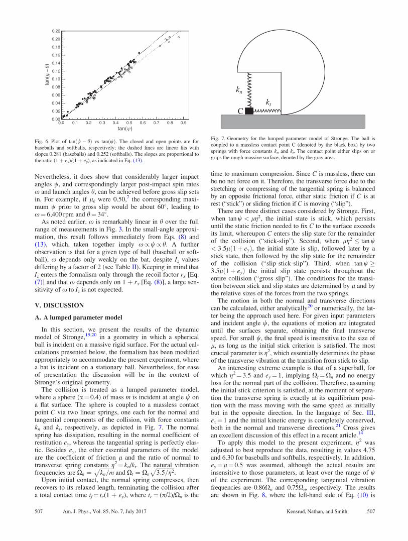
Nevertheless, it does show that considerably larger impactangles w, and correspondingly larger post-impact spin ratesx and launch angles h, can be achieved before gross slip setsin. For example, if lk were 0.50,7 the corresponding maxi-mum w prior to gross slip would be about 60�, leading tox¼ 6,400 rpm and h¼ 34�.

As noted earlier, x is remarkably linear in h over the fullrange of measurements in Fig. 3. In the small-angle approxi-mation, this result follows immediately from Eqs. (8) and(13), which, taken together imply x/w/ h. A furtherobservation is that for a given type of ball (baseball or soft-ball), x depends only weakly on the bat, despite Iz valuesdiffering by a factor of 2 (see Table II). Keeping in mind thatIz enters the formalism only through the recoil factor rx [Eq.(7)] and that x depends only on 1 þ rx [Eq. (8)], a large sen-sitivity of x to Iz is not expected.

V. DISCUSSION

A. A lumped parameter model

In this section, we present the results of the dynamicmodel of Stronge,19,20 in a geometry in which a sphericalball is incident on a massive rigid surface. For the actual cal-culations presented below, the formalism has been modifiedappropriately to accommodate the present experiment, wherea bat is incident on a stationary ball. Nevertheless, for easeof presentation the discussion will be in the context ofStronge’s original geometry.

The collision is treated as a lumped parameter model,where a sphere (a¼ 0.4) of mass m is incident at angle w ona flat surface. The sphere is coupled to a massless contactpoint C via two linear springs, one each for the normal andtangential components of the collision, with force constantskn and kt, respectively, as depicted in Fig. 7. The normalspring has dissipation, resulting in the normal coefficient ofrestitution ey, whereas the tangential spring is perfectly elas-tic. Besides ey, the other essential parameters of the modelare the coefficient of friction l and the ratio of normal totransverse spring constants g2¼ kn/kt. The natural vibrationfrequencies are Xn ¼

ffiffiffiffiffiffiffiffiffiffikn=m

pand Xt ¼ Xn

ffiffiffiffiffiffiffiffiffiffiffiffiffi3:5=g2

p.

Upon initial contact, the normal spring compresses, thenrecovers to its relaxed length, terminating the collision aftera total contact time tf¼ tc(1 þ ey), where tc¼ (p/2)/Xn is the

time to maximum compression. Since C is massless, there canbe no net force on it. Therefore, the transverse force due to thestretching or compressing of the tangential spring is balancedby an opposite frictional force, either static friction if C is atrest (“stick”) or sliding friction if C is moving (“slip”).

There are three distinct cases considered by Stronge. First,when tan w < lg2, the initial state is stick, which persistsuntil the static friction needed to fix C to the surface exceedsits limit, whereupon C enters the slip state for the remainderof the collision (“stick-slip”). Second, when lg2 � tan w< 3:5lð1þ eyÞ, the initial state is slip, followed later by astick state, then followed by the slip state for the remainderof the collision (“slip-stick-slip”). Third, when tan w �3:5lð1þ eyÞ the initial slip state persists throughout theentire collision (“gross slip”). The conditions for the transi-tion between stick and slip states are determined by l and bythe relative sizes of the forces from the two springs.

The motion in both the normal and transverse directionscan be calculated, either analytically20 or numerically, the lat-ter being the approach used here. For given input parametersand incident angle w, the equations of motion are integrateduntil the surfaces separate, obtaining the final transversespeed. For small w, the final speed is insensitive to the size ofl, as long as the initial stick criterion is satisfied. The mostcrucial parameter is g2, which essentially determines the phaseof the transverse vibration at the transition from stick to slip.

An interesting extreme example is that of a superball, forwhich g2¼ 3.5 and ey¼ 1, implying Xt¼Xn and no energyloss for the normal part of the collision. Therefore, assumingthe initial stick criterion is satisfied, at the moment of separa-tion the transverse spring is exactly at its equilibrium posi-tion with the mass moving with the same speed as initiallybut in the opposite direction. In the language of Sec. III,ex¼ 1 and the initial kinetic energy is completely conserved,both in the normal and transverse directions.21 Cross givesan excellent discussion of this effect in a recent article.14

To apply this model to the present experiment, g2 wasadjusted to best reproduce the data, resulting in values 4.75and 6.30 for baseballs and softballs, respectively. In addition,ey¼l¼ 0.5 was assumed, although the actual results areinsensitive to those parameters, at least over the range of wof the experiment. The corresponding tangential vibrationfrequencies are 0.86Xn and 0.75Xn, respectively. The resultsare shown in Fig. 8, where the left-hand side of Eq. (10) is

Fig. 6. Plot of tanðw� hÞ vs tanðwÞ. The closed and open points are for

baseballs and softballs, respectively; the dashed lines are linear fits with

slopes 0.281 (baseballs) and 0.252 (softballs). The slopes are proportional to

the ratio (1 þ ex)/(1 þ ey), as indicated in Eq. (13).

Fig. 7. Geometry for the lumped parameter model of Stronge. The ball is

coupled to a massless contact point C (denoted by the black box) by two

springs with force constants kn and kt. The contact point either slips on or

grips the rough massive surface, denoted by the gray area.

507 Am. J. Phys., Vol. 85, No. 7, July 2017 Kensrud, Nathan, and Smith 507

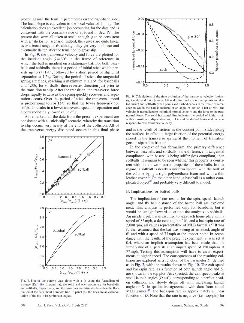
plotted against the term in parentheses on the right-hand side.The local slope is equivalent to the local value of 1 þ ex. Thecalculation does an excellent job accounting for the data and isconsistent with the constant value of ex found in Sec. IV. Thepresent data were all taken at small enough w to be consistentwith a “stick-slip” scenario. Indeed, the curves are quite linearover a broad range of w, although they get very nonlinear andeventually flatten after the transition to gross slip.

In Fig. 9, the transverse velocity and force are plotted forthe incident angle w¼ 30�, in the frame of reference inwhich the ball is incident on a stationary bat. For both base-balls and softballs, there is a period of initial stick which per-sists up to t� 1.4tc, followed by a short period of slip untilseparation at 1.5tc. During the period of stick, the tangentialspring stretches, reaching a maximum at 1.16tc for baseballsand 1.33tc for softballs, then reverses direction just prior tothe transition to slip. After the transition, the transverse forcedrops rapidly to zero as the spring quickly recovers and sepa-ration occurs. Over the period of stick, the transverse speedis proportional to cosðXttÞ, so that the lower frequency forsoftballs results in a lower transverse speed at separation anda correspondingly lower value of ex.

As remarked, all the data from the present experiment areconsistent with a “stick-slip” scenario, whereby the transitionto slip occurs very nearly at the end of the collision. All ofthe transverse energy dissipated occurs in this final phase and is the result of friction as the contact point slides along

the surface. In effect, a large fraction of the potential energystored in the transverse spring at the moment of transitiongets dissipated in friction.

In the context of this formalism, the primary differencebetween baseballs and softballs is the difference in tangentialcompliance, with baseballs being stiffer (less compliant) thansoftballs. It remains to be seen whether this property is consis-tent with the known material properties of these balls. In thatregard, a softball is nearly a uniform sphere, with the bulk ofthe volume being a rigid polyurethane foam and with a thinleather cover.22 On the other hand, a baseball is a rather com-plicated object23 and probably very difficult to model.

B. Implications for batted balls

The implication of our results for the spin, speed, launchangle, and fly ball distance of the batted ball are explorednext. This analysis is performed only for baseballs, but itwould be straightforward to extend the analysis to softballs.An incident pitch was assumed to approach home plate with aspeed of 85 mph, a descent angle of 6�, and a backspin rate of2,000 rpm, all values representative of MLB fastballs.24 It wasfurther assumed that the bat was swung at an attack angle of6� and with a speed of 73 mph at the impact point. In accor-dance with the results of the present experiment, ex was set at0.4, where an implicit assumption has been made that thesame value of ex persists at an impact speed of 158 mph as at77 mph. Testing this assumption will have to await experi-ments at higher speed. The consequences of the resulting col-lision are explored as a function of the parameter D, definedas in Fig. 2, with the results shown in Fig. 10. The exit speedand backspin rate, as a function of both launch angle and D,are shown in the top plot. As expected, the exit speed peaks atsmall launch angles (D� 0), corresponding to a perfect head-on collision, and slowly drops off with increasing launchangle or D, in qualitative agreement with data from actualMLB games.25 The backspin rate is approximately a linearfunction of D. Note that the rate is negative (i.e., topspin) for

Fig. 8. Plot of the current data along with a fit using the formalism of

Stronge (Ref. 19). In panel (a), the solid and open points are for baseballs

and softballs, respectively, and the error bars are estimates based on the fluc-

tuation of the data about a smooth line. In panel (b), the lines are an extrapo-

lation of the fits to larger impact angles.

Fig. 9. Calculations of the time evolution of the transverse velocity (points,

right scale) and force (curves, left scale) for baseballs (closed points and dot-

ted curve) and softballs (open points and dashed curve) in the frame of refer-

ence in which the ball is incident at an angle of 30� on a bat at rest. The

velocity is normalized to the initial normal velocity and the force to the peak

normal force. The solid horizontal line indicates the period of initial stick,

with a transition to slip at about t/tc¼ 1.4, and the dashed horizontal line cor-

responds to zero transverse velocity.

508 Am. J. Phys., Vol. 85, No. 7, July 2017 Kensrud, Nathan, and Smith 508

D¼ 0, a consequence of the incident backspin of the pitch.The bottom plot shows the resulting trajectory, calculatedfrom the exit speed, launch angle, and backspin, using dragand lift coefficients previously determined.26 The trajectoryevolves from a hard-hit line drive at small D, to a 400-ft homerun at intermediate D, to a lazy fly ball or popup at still largerD. These results conform nicely with observations of trajecto-ries from MLB games.27

VI. SUMMARY AND CONCLUSIONS

Experiments have been made by colliding a swinging batwith a stationary baseball and softball. The pre-impact velocityof the bat (speed and direction) was measured along with thepost-impact velocity and spin of the ball. The data have beenanalyzed to determine the tangential coefficient of restitutionof each type of ball. Both baseballs and softballs have spinsthat are enhanced relative to that expected for a rigid body,suggesting tangential compliance. In the context of a simplelumped-parameter model of the collision, it is shown that soft-balls have a greater tangential compliance than baseballs.

ACKNOWLEDGMENTS

The authors thank the group from Rawlings SportingGoods–Jarden Team Sports, including Biju Mathew, Wes

Lukash, and Chris Flahan, for the use of their facility andhelp with the data collection. The authors also thank JacobDahl, Bryant Leung, and Sam Smith from the WSU SportsScience Laboratory for their help with the data collectionand reduction.

a)Electronic mail: jkensrud@gmail.comb)Electronic mail: a-nathan@illinois.educ)Electronic mail: lvsmith@mme.wsu.edu1For a nice synopsis of the history of Rutherford’s scattering experiment,

see <http://galileo.phys.virginia.edu/classes/252/Rutherford_Scattering/

Rutherford_Scattering.html>.2An excellent reference is Jerome Friedman’s 1990 Nobel Lecture, <http://

www.nobelprize.org/nobel_prizes/physics/laureates/1990/friedman-lecture.

pdf>.3A very illuminating video called The Structure of the Proton is available at

<https://www.youtube.com/watch?v¼vtc3qbpHRPg>.4A. P. French and M. G. Ebison, Introduction to Classical Mechanics(Kluwer Academic Publishers, Norwell MA, 1986), pp. 95–123.

5G. S. Sawicki, M. Hubbard, and W. J. Stronge, “How to hit home runs:

Optimum baseball swing parameters for maximum range trajectories,”

Am. J. Phys. 71, 1152–1162 (2003).6R. G. Watts and S. Baroni, “Baseball-bat collisions and the resulting tra-

jectories of spinning balls,” Am. J. Phys. 57, 40–45 (1989).7R. Cross and A. M. Nathan, “Scattering of a baseball by a bat,” Am. J.

Phys. 74, 896–904 (2006).8Alan M. Nathan, Jonas Cantakos, Russ Kesman, Biju Mathew, and Wes

Lukash, “Spin of a batted baseball,” Procedia Eng. 34, 182–187 (2012).9Jeffrey R. Kensrud and Lloyd V. Smith, “Spin from oblique impact of bat-

ted sports balls,” Procedia Eng. 60, 130–135 (2013).10More information on ProAnalyst video analysis software is available at

<http://www.xcitex.com/proanalyst-motion-analysis-software.php>.11J. W. Then and K. Chiang, “Experimental determination for moments of

inertia by the bifilar pendulum method,” Am. J. Phys. 38, 537–539 (1970).12H. Brody, “The moment of inertia of a tennis ball,” Phys. Teach. 43,

503–505 (2005).13In collision theory, D is referred to as the impact parameter.14R. Cross, “Impact behavior of a superball,” Am. J. Phys. 83, 238–248

(2015).15A. M. Nathan, “Characterizing the performance of baseball bats,” Am. J.

Phys. 71, 134–143 (2003).16L. V. Smith, “Progress in measuring the performance of baseball and soft-

ball bats,” Sports Technol. 1, 291–299 (2009).17R. Cross, “Grip-slip behavior of a bouncing ball,” Am. J. Phys. 70,

1093–1102 (2002).18N. Maw, J. R. Barber, and J. N. Fawcett, “The role of elastic tangential

compliance in oblique impact,” J. Lubrication Technol. 103, 74–80

(1981); available at http://tribology.asmedigitalcollection.asme.org/

pdfaccess.ashx?ResourceID=4657090&PDFSource=13.19W. Stronge, Impact Mechanics (Cambridge U.P., Cambridge, UK, 2000).20W. Stronge, “Planar impact of rough compliant bodies,” Int. J. Impact

Eng. 15, 435–450 (1994).21R. Garwin, “Kinematics of an ultraelastic rough ball,” Am. J. Phys. 37,

88–92 (1969).22S. Burbank and L. V. Smith, “Dynamic characterization of rigid foam

used in finite element sports ball simulations,” Sports Eng. Technol. 226,

77–85 (2012).23P. Drane, J. Sherwood, J. Jones, and T. Connelly, “The effect of baseball

construction on the game of baseball,” Eng. Sport 7, 681–688 (2008);

available at https://scholar.googleusercontent.com/scholar?q=cache:

fzjzKFnMVj4J:scholar.google.com/+drane+baseball+construction&hl=

en&as_sdt=0,14.24A. M. Nathan, “Optimizing the swing,” The Hardball Times; <http://

www.hardballtimes.com/optimizing-the-swing/> (2015).25A. M. Nathan, “Exit speed and home runs,” The Hardball Times; <http://

www.hardballtimes.com/exit-speed-and-home-runs/> (2016).26The model used to calculate the trajectories is described on the web site of

one of the authors, <http://baseball.physics.illinois.edu/trajectory-calculator-

new.html>, and includes a link to a spreadsheet for doing the calculations.27A. M. Nathan, “Going deep on goin’ deep,” The Hardball Times; <http://

www.hardballtimes.com/going-deep-on-goin-deep/> (2016).

Fig. 10. Calculations of the ball-bat collision and the subsequent trajectories.

(a) The exit speed (the solid line, left scale) and backspin rate (the dashed

line, right scale) as a function of both D and launch angle h. (b) The trajecto-

ries for various values of D, indicated next to each curve.

509 Am. J. Phys., Vol. 85, No. 7, July 2017 Kensrud, Nathan, and Smith 509