Gravity 7

Objectives

Background

Outer Zone

Inner Zone

DEMs

EOMA

Gravity 7The Terrain Correction

Chuck Connor, Laura Connor

Potential Fields Geophysics: Terrain Week

Gravity 7

Gravity 7

Objectives

Background

Outer Zone

Inner Zone

DEMs

EOMA

Objectives for Terrain Week

• Learn about theterrain correction

• The inner terraincorrection

• Learn about DEMs

• The outer terraincorrection

• Make a terraincorrection to gravitydata

Gravity 7

Gravity 7

Objectives

Background

Outer Zone

Inner Zone

DEMs

EOMA

Background on terrain correction

Terrain corrections deal with the deviation of actual topography from the topography approximated by theBouguer slab, or spherical Bouguer cap. Consider this highly simplified diagram:

A gravity station is located at height h, corresponding to the Bouguer slab (shaded area in panel b).However, the valleys (area A in panel c) are overcompensated by the Bouguer slab. That is, the mass of theBouguer slab includes the area in the valley where the mass is absent. Similarly, the mass at the top of thehill (area B in panel c) pulls up on the gravity meter but is not accounted for by the simple Bouguercorrection. The terrain correction is designed to account for the effects of “real world” topography.

Effect of topography

Note that the effect of valleys is that the simple Bouguer slab correction has removed the effect of mass thatwas not there to begin with. Therefore after the terrain correction is applied, the terrain corrected gravityshould be greater than the simple Bouguer gravity. Likewise, the hilltop, unaccounted for in the simpleBouguer correction, pulls up on the gravity meter. Therefore, like the valley, after the terrain correction isapplied, the terrain corrected gravity due to the hilltop should be greater than the simple Bouguer gravity.

Gravity 7

Gravity 7

Objectives

Background

Outer Zone

Inner Zone

DEMs

EOMA

Background on terrain correction

The complex topography of the Medicine Lake (CA)highlands, with its lava domes, cones, and faults,illustrates the potential significance of deviation froma simple Bouguer slab model of topography.

Apparently the terrain correction was first consideredby Hayford and Bowie, around 1912, in interpretinggravity anomalies in the US. The problem of how toestimate the terrain correction was tackled by thegeodesists Cassinis, Bullard, and Lambert in the1930s. Hammer developed a practical approach forperforming terrain corrections out to about 22 kmfrom the station.

Bullard (1936) broke the topographic correction intothree parts. The first two are the Bouguer correction(Bullard A), which approximates the topography to aninfinite horizontal slab of thickness equal to the heightof the station above the reference ellipsoid or anotherdatum plane, and the curvature of the Earth (BullardB) or spherical cap, which reduces the infiniteBouguer slab a spherical cap of the same thickness,with a surface radius of 166.735 km – 1.5 degree. Wehave already discussed these corrections in Module 5.

The third correction (Bullard C) is the terraincorrection which takes undulations of topography intoaccount. Topographic variations results in theupwards attraction of hills above the plane of thestation and valleys below, which decrease the observedvalue of gravity, so both of these effects must beadded to readings to correct for topography.

Gravity 7

Gravity 7

Objectives

Background

Outer Zone

Inner Zone

DEMs

EOMA

The Hammer Net

Hammer improved on the method of Hayford to simplify terrain corrections. His “Hammer net” was used for70 yr to make terrain corrections. The method involves compartmentalizing the area surrounding themeasurement point using a template – the Hammer net. The net is used with printed topographic maps.Radial lines from the gravity station extend from the center of the net, and concentric circles drawn atspecific distances from the gravity station, consistent with the scale of the topographic map. An averageelevation above or below the station elevation within each compartment is estimated.

gcomp = Gρ∆θ

[Ro − Ri +

√R2

i + h2 −√R2

o + h2]

where: ρ is the bulk density of the terrain used in the simple or spherical cap Bouguer correction, h is theheight difference of the compartment, ∆θ is the angle subtended by the two radial lines bounding thesegment, Ri and Ro are the outer and inner radii bounding the compartment. This is the gravity effect of aradial segment of a hollow vertical cylinder, with a flat top (the average elevation difference with the station,h). The gravitational effect of each compartment is then summed to estimate the terrain correction:

gter =N∑

k=1

gcomp

where: N is the total number of compartments.

Although Hammer nets are no longer used, generally, this method illustrates the same basic concept still usedin computer programs to estimate the terrain correction. That is, elevation data are found as a function ofdistance and direction from each gravity station, and the gravitational effect of the elevation difference iscalculated as a function of distance.

Gravity 7

Gravity 7

Objectives

Background

Outer Zone

Inner Zone

DEMs

EOMA

The Hammer Net

A Hammer net, or similar net used by a computer program looks like this:

1 2 3 4 5 6 70◦

15◦

30◦

45◦

60◦

75◦90◦

105◦

120◦

135◦

150◦

165◦

180◦

195◦

210◦

225◦

240◦

255◦270◦

285◦

300◦

315◦

330◦

345◦

Ri

Ro

hi

ho

For each terrain correction, the net iscentered on the gravity station (reddot) and the elevation of the station,hs is determined, using the terrainmodel. The elevation difference witheach compartment is then estimated.A simple scheme is:

h′i = hs − hi

h′o = hs − ho

h =h′i + h′o

2

Note that the innermost zone is aspecial case, because hs = hi andbecause the correction is mostsensitive to topographic variations inthis inner zone. Consequently adifferent inner zone correction isnormally used and the Hammer net -like corrections are referred to a outerzone terrain corrections. Usually theinner zone is of 50 m radius, or so.

Gravity 7

Gravity 7

Objectives

Background

Outer Zone

Inner Zone

DEMs

EOMA

A simplified example of the Hammer Net

Example

What is the terrain effect of a lava dome range of average relief 500 m located 2–5 km from the gravitymeter, S? Assume the dome is contained in a compartment defined by ∆θ = 45◦.

gcomp = Gρ∆θ

[Ro − Ri +

√R2

i + h2 −√R2

o + h2]

with G = 6.67 × 10−11 N m2 kg−2, ρ = 2300 kg m−3, ∆θ = π/4, Ri = 2000 m, Ro = 5000 m:

gcomp = 0.44 mGal

Ro

Ri

∆θ

S

lava domeh = 500 m

First, realize that this is a substantial effect. If agravity map were made across the region, the simpleBouguer anomaly would have a gravity gradient,increasing away from the volcano. Also, sincetopographic features do not occur in isolation, thecumulative effect of topography may be much larger.Second, note that, although this calculation is quitecoarse compared to an actual terrain correction, it ispossible in the field to quickly and roughly estimatethe expected gravitational effect of topographicfeatures with a topographic map and compass.

Gravity 7

Gravity 7

Objectives

Background

Outer Zone

Inner Zone

DEMs

EOMA

The inner zone terrain correction

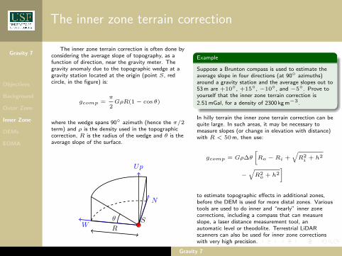
The inner zone terrain correction is often done byconsidering the average slope of topography, as afunction of direction, near the gravity meter. Thegravity anomaly due to the topographic wedge at agravity station located at the origin (point S, redcircle, in the figure) is:

gcomp =π

2GρR(1 − cos θ)

where the wedge spans 90◦ azimuth (hence the π/2term) and ρ is the density used in the topographiccorrection, R is the radius of the wedge and θ is theaverage slope of the surface.

N

W

Up

R

θ S

Example

Suppose a Brunton compass is used to estimate theaverage slope in four directions (at 90◦ azimuths)around a gravity station and the average slopes out to53 m are +10◦, +15◦, −10◦, and −5◦. Prove toyourself that the inner zone terrain correction is

2.51 mGal, for a density of 2300 kg m−3.

In hilly terrain the inner zone terrain correction can bequite large. In such areas, it may be necessary tomeasure slopes (or change in elevation with distance)with R < 50 m, then use:

gcomp = Gρ∆θ

[Ro − Ri +

√R2

i + h2

−√R2

o + h2

]

to estimate topographic effects in additional zones,before the DEM is used for more distal zones. Varioustools are used to do inner and “nearly” inner zonecorrections, including a compass that can measureslope, a laser distance measurement tool, anautomatic level or theodolite. Terrestrial LiDARscanners can also be used for inner zone correctionswith very high precision.

Gravity 7

Gravity 7

Objectives

Background

Outer Zone

Inner Zone

DEMs

EOMA

Working with Digital Elevation Models

In practice, the outer zone terrain correction ismade using a digital elevation model (DEM). This is aDEM of the Medicine Lake volcano area (California): Steps in getting and using a DEM include:

• download the DEM data. Globally, DEM dataare available at 90-m-resolution derived fromshuttle radar topography mission (SRTM)data. In many countries, such as the US,30-m or 10-m DEM data are readily available.

• Most outer terrain correction codes use aUTM Grid (in meters) rather than latitude /longitude coordinate system (in degrees) . Soit is necessary to convert the DEM, usually,from lat/long to UTM. Program such asProj4, ArcGIS, or gdal can used to do thisconversion.

• The terrain model must be checked, so thatthere are no “holes” in the DEM or missingvalues. These missing values can causesignificant errors in terrain corrections usingDEMs.

• Usually the data are re-gridded to getregularly spaces rows and columns of elevationvalues over the region of interest.

Gravity 7

Gravity 7

Objectives

Background

Outer Zone

Inner Zone

DEMs

EOMA

Additional Reading

The book by Hinze et al. (2013) has an excellent overview of the terrain correction. Various authors haveworked on the terrain correction, proposing verious inner zone and outer zone corrections. Important paperson the topic include:

• Hammer, S. (1939). Terrain corrections for gravimeter stations. Geophysics, 4(3), 184–194.

• Kane, M. F. (1962). A comprehensive system of terrain corrections using a digital computer.Geophysics, 27(4), 455–462.

• Nowell, D. A. G. (1999). Gravity terrain correctionsaan overview. Journal of Applied Geophysics,42(2), 117–134.

• Campbell, D. L. (1980). Gravity terrain corrections for stations on a uniform slope-A power lawapproximation. Geophysics, 45(1), 109–112.

• Banerjee, P. (1998). Gravity measurements and terrain corrections using a digital terrain model inthe NW Himalaya. Computers Geosciences, 24(10), 1009–1020.

• Cogbill, A. H. (1990). Gravity terrain corrections calculated using digital elevation models.Geophysics, 55(1), 102–106.

Gravity 7

Gravity 7

Objectives

Background

Outer Zone

Inner Zone

DEMs

EOMA

End of Module Assignment

1 Suppose you set up the gravity meter to take a measurement next to a curb, 0.2 m in relief. Assumethe gravity meter center is 0.2 m from the actual curb edge. Use the inner zone formula to estimatethe terrain effect of the curb. Note: assume the curb is straight, so that two 90-degree wedges of theinner zone are above the curb, and two 90-degree wedges are below the curb. Explain your result,including the density value you assume.

2 Suppose you set up a gravity station and you use a laser rangefinder to estimate the vertical heightdifference between the meter and the ground surface at a horizontal distance of 53 m from the gravitymeter in four cardinal directions. These height differences are: 10 m, -5 m -4 m and 8 m. What is theinner zone terrain correction? Explain your result, including the density value you assume.

3 Suppose you set up a gravity station approximately 30 km from Mt Shasta volcano. The relief of Mt.Shasta is approximately 3000 m and the diameter approximately 20 km. Estimate the terrain effect ofMt. Shasta on your gravity reading. Explain your result, including the density value you assume.

Gravity 7

Gravity 7

Objectives

Background

Outer Zone

Inner Zone

DEMs

EOMA

EOMA

4 The outer zone correction can be estimated using the PERL script: terrain corr2.pl. This code usesthe “Hammer” formula (hollow right vertical cylinder) to estimate the terrain correction using aconfiguration file and a digital elevation model. The configuration file specifies the informationneeded to run the code. This includes:(1) The name of the file containing the gravity data to be corrected. In this case, use the file:“gravity data 62E ...utm”. This file lists Medicine Lake area gravity values by utm coordinate,simple Bouguer gravity reading, and elevation.(2) The name of the digital elevation model (DEM) file to be used to make the terrain correction.(3) The angular frequency, ∆θ with which terrain corrections are made.(4) the thickness of the hollow cylinders used in the terrain correction (distance between Ro andRi).(5) the “skip distance”, that is the distance from the gravity meter to the first value of Ri. Terrainin this zone is not corrected for as this is defined as the inner zone.(6) the limits of the DEMThe values shown in the configuration file can be edited to change the terrain correction. Use the90-m and 30-m DEM files provided to estimate the terrain correction for the Medicine Lake gravitystations. How does the terrain correction change for the gravity stations with change in theresolution of the DEM (from 30 to 90 m)? Using the 30 m DEM, how does the terrain correctionchange with the angular frequency, ∆θ, and with the distance between Ro and Ri? Summarizeyour results graphically and explain them!

Gravity 7