objective optimization of weather radar networks for low-level...

Objective Optimization of Weather Radar Networks for Low-Level CoverageUsing a Genetic Algorithm

JAMES M. KURDZO AND ROBERT D. PALMER

School of Meteorology, and Atmospheric Radar Research Center, University of Oklahoma, Norman, Oklahoma

(Manuscript received 8 April 2011, in final form 22 November 2011)

ABSTRACT

The current Weather Surveillance Radar-1988 Doppler (WSR-88D) radar network is approaching 20 years

of age, leading researchers to begin exploring new opportunities for a next-generation network in the United

States. With a vast list of requirements for a new weather radar network, research has provided various

approaches to the design and fabrication of such a network. Additionally, new weather radar networks in

other countries, as well as networks on smaller scales, must balance a large number of variables in order to

operate in the most effective way possible. To offer network designers an objective analysis tool for such

decisions, a coverage optimization technique, utilizing a genetic algorithm with a focus on low-level coverage,

is presented. Optimization is achieved using a variety of variables and methods, including the use of clima-

tology, population density, and attenuation due to average precipitation conditions. A method to account for

terrain blockage in mountainous regions is also presented. Various combinations of multifrequency radar

networks are explored, and results are presented in the form of a coverage-based cost–benefit analysis, with

considerations for total network lifetime cost.

1. Introduction

As the current Weather Surveillance Radar-1988

Doppler (WSR-88D) radar network approaches the end

of its expected lifetime (Yussouf and Stensrud 2008),

numerous studies have raised several opportunities for

improvement in a future network. Of principle interest is

decreasing the time needed to complete a full volume

scan in order to provide forecasters with more time and

data for issuing warnings. Multiple proposals for a new

Multimission Phased Array Radar (MPAR) network

have attempted to address this desire (Weber et al. 2007;

Zrnic et al. 2007). Additionally, improvements in the low-

level scanning height in a new radar network are possible if

the operational range of individual radars is less than the

current 460-km range of the WSR-88D systems and radar

sites are located closer to each other. The Collaborative and

Adaptive Sensing of the Atmosphere (CASA) program

proposes the use of low-cost X-band polarimetric radars

that could be placed less than 20 km apart in order to

observe a greater portion of the boundary layer nationwide

(McLaughlin et al. 2009). Additionally, the CASA concept

aims to provide collaborative, adaptive capabilities in

a weather radar network, resulting in faster scan updates

for the most weather-impacted areas. Such a network could

also be capable of providing low-level wind field observa-

tions for rapid-update mesoscale models, in order to pro-

vide warn-on-forecast support for the National Weather

Service (Stensrud et al. 2009).

Whether long-range S-band radars or shorter-range

X-band radars (or a combination thereof) are used in

a future network, the total cost, including production,

maintenance, and operation, will be an important factor.

S-band radars, such as those currently being used in the

WSR-88D network, are typically priced at a relatively

substantial level, while X-band radars operating at a low

power are expected to cost considerably less. However,

being placed only 20 km apart, the cost of such an X-band

network may also exceed viable funding amounts solely

because of the number of radars that would be required.

Therefore, it is prudent to fabricate a network that offers

as many improvements to current networks as possible,

while remaining fiscally sound.

One option, which could offer numerous improve-

ments while potentially keeping costs low, would be to

Corresponding author address: James M. Kurdzo, Atmospheric

Radar Research Center, University of Oklahoma, 120 David L.

Boren Blvd., Suite 4600, Norman, OK 73072.

E-mail: [email protected]

JUNE 2012 K U R D Z O A N D P A L M E R 807

DOI: 10.1175/JTECH-D-11-00076.1

� 2012 American Meteorological Society

utilize a multifrequency network design in order to offer

long-range coverage for more expensive S-band sys-

tems, while supplying short-range, X-band coverage in

areas not covered at low-levels by S-band systems. A

need therefore exists to optimize such a multifrequency

network, in order to maximize coverage while mini-

mizing cost. Through a series of optimizations, a cost-

benefit analysis can be completed, informing network

designers as to the most cost-effective network possi-

bilities (in the case of this paper, ‘‘benefit’’ refers to

coverage). Other radar network designs may also gain

from similar optimizations, including single-frequency

networks aiming simply for maximum areal coverage, as

well as smaller networks optimizing for a particular

coverage field such as population.

Observation network design, and coverage optimi-

zations in general, are not new problems. Cellular

tower placement presents a very common coverage

problem, which has been solved in a variety of ways

(e.g., Raisanen and Whitaker 2003; Thornton et al.

2003; Amaldi et al. 2008). Because of the large, com-

plex nature of cellular networks, simulation tools are

not sufficient; optimization algorithms [specifically

genetic algorithms (GAs)] are capable of handling

these problems (Lieska et al. 1998). Lieska et al. (1998)

argued that genetic algorithms process the computer’s

representation of potential solutions directly, leading to

a more rapid convergence to a solution. A fixed number

of base stations (possible siting locations) in a gridded

format were used, further limiting the computational

complexity.

Genetic algorithms have also been used by Du and

Bigham (2003) for cellular network optimization, with

a specific emphasis on balancing traffic load using geo-

graphic variables. The study focused on optimizing

coverage sizes and shapes in order to efficiently handle

common traffic demand patterns. It was found that with

the correct input parameters, genetic algorithms pro-

vided a relatively rapid convergence to an acceptable

solution. Jourdan and de Weck (2004) also concluded,

through significant review of various optimization

methods, that genetic algorithms were the most suitable

fit for a coverage study in which grid points are pre-

determined for coverage testing. In their case, the goal

was to develop coverage patterns for aircraft-dropped,

ad hoc wireless sensor networks.

In terms of weather radar network planning, there is

limited literature regarding coverage optimization

and radar siting using numerical methods. Leone et al.

(1989) selected WSR-88D sites based upon various

criteria, including severe weather climatology and

distance from population centers. However, numeri-

cal optimization was not used, and a relatively small

number of potential siting areas were considered. Ray

and Sangren (1983) proposed planning small, multiple-

Doppler networks for research purposes using a search

algorithm. This was feasible for relatively small radar

networks (less than 10 radars), but with the number of

variables being utilized, a more expansive network

could become problematic, simply because of the

computation time needed for exhaustive search tech-

niques.

Minciardi et al. (2003) presented the use of a genetic

algorithm for planning an Italian weather radar net-

work. Again, a relatively small number of potential sites

were identified as viable options to locate radar systems.

The advantages and disadvantages of each site were

weighted and used in an optimization problem that de-

termined the optimal placement of sensors based on the

input parameters; this was termed ‘‘site eligibility.’’ The

study was principally designed as a decision support

system, with focus on one radar frequency and a limited

set of potential siting locations.

In this paper, a genetic optimization algorithm capable of

maximizing coverage within set physical boundary condi-

tions is presented, using any combination of frequencies/

ranges, and using any two-dimensional, quantifiable field

as an optimizable quantity, such as those in Leone et al.

(1989). The algorithm is applied to numerous real-world

examples, including optimization based on combined

population density and tornado probability, open-space

coverage, and coverage with a simple terrain model.

Testing is focused on low-level coverage examples,

yielding shorter-range assumptions for low-frequency

radars. The first result is provided as a basic example,

while the remaining two results are analyzed in the form

of a cost–benefit analysis, with stress placed on the de-

cision support nature of the results, as in Minciardi et al.

(2003) and Raisanen and Whitaker (2003). Conclusions

are drawn regarding advantages and disadvantages of

using multiple frequencies in each of the last two situa-

tions.

2. Optimization framework using a geneticalgorithm

An optimal radar network must offer the most cover-

age possible, while minimizing cost, which is directly re-

lated to the number of radars. The coverage model, or

fitness function, must be accurately quantifiable, capable

of being evaluated over a large domain, and computa-

tionally inexpensive. Computational complexity results in

slow processing speeds, meaning in order to keep speeds

reasonable, it is impossible to offer every possible loca-

tion within the domain as a siting location. Because of

these necessities and limitations, a gridded format of sites

808 J O U R N A L O F A T M O S P H E R I C A N D O C E A N I C T E C H N O L O G Y VOLUME 29

was deemed to most suitably fit our needs. Over the do-

main of the optimization, a gridded system with 0.18 of

latitudinal and longitudinal spacing is defined. Each grid

point represents both a potential radar site location and

a location for testing coverage. Since this results in a finite

domain, it is plausible to expect to achieve close to

a global maximum in fitness without the need for exces-

sive computing power.

Every optimization problem has different charac-

teristics, leading to the need to explore all of the op-

timization techniques available in order to fit the needs

of the problem. There are a number of global optimi-

zation techniques available; however, it was the goal of

this work to identify one technique and develop a ro-

bust algorithm tailored to our needs. To identify the

general technique for our problem, numerous optimi-

zation methods were explored. Multistart methods

(Boender et al. 1982) utilize local optima search

techniques, with searches beginning at many points

along the solution curve. This leads to many ongoing

searches at once, and a tax on computational com-

plexity for large domain problems such as ours. Various

linear programming methods exist (Dantzig and Thapa

1997; Karmarkar 1984), including the simplex algo-

rithm (efficient method of finding a ‘‘feasible region,’’

but nondesirable results for large domains) and interior

point optimization (similar to the simplex algorithm,

but searches a greater depth of the feasible region).

Nonlinear programming methods, such as the quasi-

Newton approach (via use of gradient vectors), Nelder–

Mead method (similar to the simplex algorithm), and the

trust-region technique (which only searches a portion of

the objective function) provide systems that allow for

nonlinear constraints, similar to those in our problem

(Shanno 1970; Nelder and Mead 1965; Celis et al. 1984).

Evolutionary algorithms represent a general concept

that encompasses numerous types of optimization

techniques (Eiben and Smith 2007). Genetic algorithms,

specifically, are designed to be capable of finding global

optimum solutions to complicated, nonlinear, real-

world problems. Additionally, genetic algorithms have

the ability to remain computationally inexpensive for

simple problems, or to be developed into sophisticated

algorithms capable of solving advanced problems.

Genetic algorithms offer one of the most consistent

methods to achieve global optimum, while also being

flexible enough to accommodate real-world boundary

conditions (Holland 1975).

The need for a global optimum, along with promising

results from Du and Bigham (2003), Jourdan and de

Weck (2004), and Lieska et al. (1998), resulted in the

choice of a genetic algorithm for optimization. Genetic

algorithms utilize the theory of evolution in order to

progressively improve the functionally defined fitness.

While it is certainly possible that other methods could

result in more accurate–timely computations, genetic

algorithms provided a reputable technique to build

a test-case algorithm for the problem at hand. In our

case, the population is defined as an array containing

the latitudinal and longitudinal coordinate for each

radar (each coordinate is a population member). In-

dividual population members are stored as a floating-

point representation (as opposed to binary), and are

altered using random number generation (as opposed

to bit replacement; Eiben and Smith 2007).

Between each generation, a portion of the pop-

ulation with the lowest fitness is discarded, and the

remaining population members are randomly paired to

create ‘‘children’’ (this is termed ‘‘crossover’’). A key

feature of genetic algorithms is the ability to avoid

local maxima in fitness. To achieve this, occasional

mutations are introduced with a predetermined like-

lihood of occurrence. Additionally, in order to guar-

antee the lack of regression in fitness, the top two

population members with the highest fitness, or ‘‘elite

members,’’ are retained through each generation.

Generations continue until a maximum fitness score is

obtained; this maximum is recognized by a lack of change

in the best fitness score for a predetermined number of

generations, indicating convergence to a solution, and the

end of the optimization.

A unique strength of the GA framework is the ability

to apply the technique to a wide variety of real-world

problems. In addition, in the case of a network cov-

erage problem, there are various ways to represent

population members and a fitness function. For the

application presented here, a gridded system is uti-

lized, which has numerous advantages. First, the

search field can be limited to a domain as large or as

small as computationally feasible. Second, boundary

conditions can be easily imposed. Last, a gridded do-

main allows for unique applications of coverage and

fitness function representations, making it simple to

add value to the coverage problem. Each of these ad-

vantages will be explored in depth in the following

discussion.

The application of a grid for the case at hand in-

volves using a simple binary system to assess coverage.

The gridded resolution used is 0.18 of latitude and

longitude. Each point along the grid represents both

a possible siting location and a location to assess cov-

erage. This means that any radar can be located (its

center coordinates) at a latitudinal and longitudinal

position that is a multiple of the 0.18 resolution. When

a radar is placed at a site, a theoretical circle is drawn

that represents the expected range of the given radar.


This range may be based on power return degradation

or the desired maximum height of the radar beam

above ground level. For example, the range of a WSR-

88D S-band radar is approximately 460 km; however,

if low-level coverage is desired, the vertical cutoff

height may be 1 km, effectively limiting the range of

the radar to approximately 75 km.

After the circle for coverage is drawn for a radar site,

the algorithm tests all grid points in order to determine

if they are encompassed in the circle. If a point is in the

circle, it is assigned a value of one. If it is not within the

circle, it is assigned a value of zero. This simple, binary

encoding technique allows for rapid computation of

coverage for not only one radar, but all of the radars

that may be placed inside the domain. The fitness

function used sums the values of all of the grid points,

resulting in a higher fitness score when more points are

covered. This means that if multiple radars are over-

lapping, successive generations will work to ‘‘spread’’

the radars in order to provide more covered points. In

this fashion, accounting for overlapping coverage as

a penalty is not necessary, further reducing the com-

putational complexity of the algorithm. A graphical

representation of the fitness function and gridded sys-

tem is shown in Fig. 1.

By limiting the number of grid points used for

placing radars and testing for coverage to 0.18 resolu-

tion, the total search space can be limited significantly,

leading to reduced computational complexity. While

this system uses binary variables for each grid point, it

is also possible to enhance the fitness score based upon

weighted ‘‘fields.’’ These enhancements allow a de-

signer to optimize a network based on very specific

needs, and the gridded system is an integral part of the

capability to perform such optimizations. The pop-

ulation members are represented via a concatenated

array that contains the latitudinal and longitudinal

coordinates for each radar in the optimization. Each

member represents one set of radar locations, resulting

in one fitness score for each network. As the members

are combined and mutated through generations, new

sets of radar locations are created in order to test for

more optimal solutions. Figure 2 offers a concise de-

scription of the steps the algorithm takes in order to

reach an optimal solution.

For each case presented, a population size of 750 and

an elite count of two are used. Of the remaining 748

population members in the generation, approximately

80% are created via crossover, and approximately

20% are created via mutation. The genetic algorithm

places a set number of radars at each frequency inside

the gridded domain, while the fitness function de-

termines which points are covered at each generation.

The fitness function improves for each point that is

covered by a radar, resulting in a ‘‘spreading’’ effect of

the radar locations; this effectively maximizes cover-

age for the given number of radars. The grid can be

enhanced using similarly gridded datasets (or fields),

which add value to specific locations. The use of fields

will be explored in the first example in section 3.

3. Representative optimization examples

This paper provides three example optimizations,

illustrating the flexibility and scope of the algorithm.

The first example utilizes both severe weather clima-

tology and population density data to optimize a small,

dual-frequency network. The second takes into ac-

count X-band attenuation due to average convective

rainfall as observed by the Oklahoma Mesonet in the

design of a dual-frequency network. The third example

demonstrates the ability to incorporate terrain block-

age in combined mountainous/flat regions while also

optimizing a dual-frequency network. These examples

are summarized in Table 1. This section describes the

data acquisition, methodology, and results used for

each example.

FIG. 1. Graphical representation of real-world boundaries,

gridded system, and the method of determining fitness. In a bi-

nary example, each of the grid points colored red would be as-

signed a value of 1 (covered by a radar), and each of the grid

points colored blue would be assigned a value of 0. The fitness is

determined by adding up these gridpoint values. Also note that

each grid point also serves as a potential siting location, limiting

the possible sites to a more manageable number for computation.


a. Population density and tornado climatology: Anillustrative example in Indiana

A key feature of the optimization algorithm is the

ability to optimize spatially with the aid of a ‘‘field,’’

which can be adapted to the grid spacing being used

for potential sites. Fields alter the binary system of

assessing radar coverage by weighting the fitness score

based upon a predetermined variable. A basic exam-

ple is a multiplicative field of population density and

tornado climatology. This results in one optimizable

field, which is superimposed over the entire domain to

be optimized.

It should be emphasized that the algorithm is flexible

enough to accommodate a vast number of possible ex-

amples beyond those shown in the following sections.

There are a number of optimization criteria that can be

chosen for optimization; however, it can be challenging

to acquire the necessary data at a high-enough resolu-

tion for accurate analysis. Tornado occurrence and

population centers are two relevant metrics that can be

easily acquired and combined, and allow for an accurate

demonstration of nonbinary weighting in a network

optimization. It is important to note that any quantifi-

able data that can be interpolated to the grid system can

be used as a field/weighting tool.

1) METHODOLOGY

Population density data are available from many

sources and in many formats. The highest resolution

data available free of charge were obtained from the

Center for International Earth Science Information

Network at Columbia University. The Gridded Pop-

ulation of the World project provides population den-

sity files spanning the entire earth at a base resolution

of 2.5 arc minutes (or approximately 0.04178) for the

year 2000 (Balk and Yetman 2004). A linear combi-

nation of Green functions, known as a biharmonic

spline interpolation method (Sandwell 1987), is used to

degrade the resolution of the data to 0.18 in order to fit

the grid spacing used by the optimization algorithm

(Fig. 3a).

Additionally, in the midwestern states of the United

States, tornado detection at low levels is a serious

concern for forecasters. Therefore, it is conceivable

that a radar network designer with limited funds would

want to weight the placement of radar systems toward

those areas more likely to be affected by tornadoes.

Tornado climatology data in the form of number of F2

tornado days per year from 1950–2009 (Brooks et al.

2003) are used for this study as input to the grid system

(Fig. 3b).

FIG. 2. Flowchart describing the genetic algorithm used for op-

timization. Fitness is determined by summing the values of the

covered grid points, with higher fitness representing a more fa-

vorable solution.

TABLE 1. Three siting optimization examples.

Type Location Height AGL X-band range Fixed radars?

Combined field Indiana 1 km 40 km WSR-88D

Attenuation Oklahoma 1 km ;25 km None

Terrain blockage Colorado 1 km 40 km None


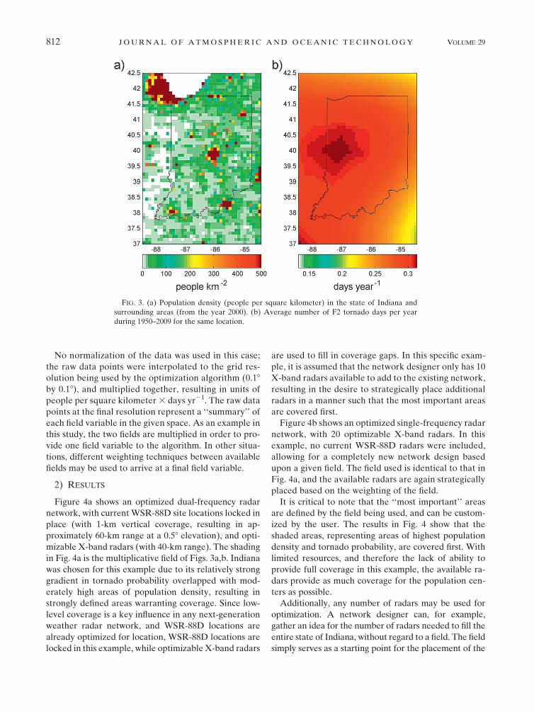
No normalization of the data was used in this case;

the raw data points were interpolated to the grid res-

olution being used by the optimization algorithm (0.18

by 0.18), and multiplied together, resulting in units of

people per square kilometer 3 days yr21. The raw data

points at the final resolution represent a ‘‘summary’’ of

each field variable in the given space. As an example in

this study, the two fields are multiplied in order to pro-

vide one field variable to the algorithm. In other situa-

tions, different weighting techniques between available

fields may be used to arrive at a final field variable.

2) RESULTS

Figure 4a shows an optimized dual-frequency radar

network, with current WSR-88D site locations locked in

place (with 1-km vertical coverage, resulting in ap-

proximately 60-km range at a 0.58 elevation), and opti-

mizable X-band radars (with 40-km range). The shading

in Fig. 4a is the multiplicative field of Figs. 3a,b. Indiana

was chosen for this example due to its relatively strong

gradient in tornado probability overlapped with mod-

erately high areas of population density, resulting in

strongly defined areas warranting coverage. Since low-

level coverage is a key influence in any next-generation

weather radar network, and WSR-88D locations are

already optimized for location, WSR-88D locations are

locked in this example, while optimizable X-band radars

are used to fill in coverage gaps. In this specific exam-

ple, it is assumed that the network designer only has 10

X-band radars available to add to the existing network,

resulting in the desire to strategically place additional

radars in a manner such that the most important areas

are covered first.

Figure 4b shows an optimized single-frequency radar

network, with 20 optimizable X-band radars. In this

example, no current WSR-88D radars were included,

allowing for a completely new network design based

upon a given field. The field used is identical to that in

Fig. 4a, and the available radars are again strategically

placed based on the weighting of the field.

It is critical to note that the ‘‘most important’’ areas

are defined by the field being used, and can be custom-

ized by the user. The results in Fig. 4 show that the

shaded areas, representing areas of highest population

density and tornado probability, are covered first. With

limited resources, and therefore the lack of ability to

provide full coverage in this example, the available ra-

dars provide as much coverage for the population cen-

ters as possible.

Additionally, any number of radars may be used for

optimization. A network designer can, for example,

gather an idea for the number of radars needed to fill the

entire state of Indiana, without regard to a field. The field

simply serves as a starting point for the placement of the

FIG. 3. (a) Population density (people per square kilometer) in the state of Indiana and

surrounding areas (from the year 2000). (b) Average number of F2 tornado days per year

during 1950–2009 for the same location.


first new radars, in order to cover the areas deemed most

important first.

b. Accounting for attenuation: Use of Mesonet datafor an Oklahoma network

A useful tool for a network optimization is the ability to

accurately represent the coverage of a given radar type

given a set of atmospheric conditions. In even moderate

precipitation cases, X-band coverage range at a reliable

sensitivity level can be significantly degraded, resulting in

the need for more radars in order to provide data for

the same area. Chandrasekar and Lim (2008) proposed

dealing with attenuation at high frequencies by in-

corporating a networked approach, leading to moment

estimates (including polarimetric variables) based

upon the returned signals to multiple radars. While this

technique is applicable to the given scenario, the optimal

placement of individual, nonoverlapping radars across

a wide domain is a key requirement for such a network to

operate. The second example is a simple coverage op-

timization, but utilizes average rainfall data to account

for attenuation at X band. This example illustrates the

difference in range between clear and precipitating

conditions for high-frequency radar systems, and how

this difference affects a cost–benefit analysis of a po-

tential multifrequency network.

1) METHODOLOGY

Oklahoma Mesonet data are utilized for this exam-

ple, and were provided by the Oklahoma Climatological

Survey (McPherson et al. 2007). To quantify average

‘‘convective season’’ precipitation, 10 years of data from

the month of May (May 2001–May 2010) were acquired.

These data contain rainfall information at 5-min resolu-

tion for well over 100 Mesonet stations across Oklahoma.

Since a change in radar sensitivity with range due to

attenuation is only a concern when it is actually pre-

cipitating, it is not sufficient to simply calculate the amount

of rain over the entire period and divide by the total time.

Instead, it is prudent to determine the average rainfall rate

only when raining. To achieve this goal, each 5-min bin is

tested for a change of at least 0.01 in. of precipitation. If

this condition is met, it is considered to have been raining

for the entire length of the 5-min bin. All 10 years of data

are processed in this matter, resulting in a total amount of

rainfall, as well as a total amount of time in which pre-

cipitation was occurring. The quotient of these numbers

results in the average rainfall rate during the month of

FIG. 4. (a) Optimized dual-frequency radar network for the state of Indiana, using a multiplicative combination

of Figs. 3a,b, fixed WSR-88D locations with 1-km vertical coverage maximum, and 10 optimizable X-band radars.

(b) Optimized single-frequency radar network for the state of Indiana, using the same field as in (a), but with 20

optimizable X-band radars.


May during 2001–10. This value is calculated for each

individual Mesonet station, and a biharmonic spline

interpolation (Sandwell 1987) is once again used to

interpolate the data to the grid spacing required for

analysis (in this case, 0.18 grid spacing is used), as shown

in Fig. 5.

Each potential site in the grid is tested for attenuation.

The weather radar equation is used to compare the

sensitivity of a nonattenuated radar to the sensitivity of

a radar that experiences losses due to the rainfall shown

in Fig. 5 (Doviak and Zrnic 1993):

Pr 5Ptg

2hctpu2l2

(4p)3r2l216 ln2, (1)

where Pr and Pt are power returned and transmitted,

respectively (W); g is gain of the antenna and l repre-

sents losses (both in dB); h is reflectivity (m21); c is the

speed of light (m s21); t is the pulse width (ms); l is

wavelength and r is range (both in m); and u is one-way

half-power beamwidth. Equation (1) can be solved for

h, which can in turn be used to calculate reflectivity

factor Z:

Z 5r2l2(4p)316 ln2Prl

2

Ptg2ctp6u2jkwj

2, (2)

where kw is the specific attenuation of water (unitless),

and Pr is set to 2110 dBm.

Figure 6 shows two profiles that solve for Z with re-

spect to r. The solid line represents a typical X-band

radar (e.g., CASA) sensitivity profile with only atmo-

spheric losses taken into account (a nonprecipitating

case). At 50 km, for example, the sensitivity of such

a radar is approximately 21 dBZ, meaning the mini-

mum return that the radar can detect is 21 dBZ. The

dashed line represents an example sensitivity profile

that takes into account both atmospheric losses and

those due to the rainfall rate profile shown. This radar

profile reaches the same sensitivity threshold as the

atmosphere-only case at 28 km, meaning that the ef-

fective range of the radar is cut by 22 km (44%).

This method can be used to compare standard,

nonprecipitating radar operating ranges to conditions

that incorporate losses due to rainfall, resulting in

different effective radar ranges. The technique in-

crementally checks to see whether the current atten-

uated range is greater than or less than the current

range being tested. If it is less, the increments stop,

and the range for the radial being tested is recorded.

This is repeated for each radial (at 1.08 increments),

resulting in a new coverage pattern for the radar site

being tested. This new pattern is based solely on the

rainfall rate and associated attenuation, resulting in

slightly different coverage patterns throughout the

state.

It is important to note that in this example, no fields

were used in the optimization; a binary weighting system

was used in the fitness function. The difference in this

example is that instead of using circles for radar repre-

sentation based upon height above ground level, the

circles plotted and used in the algorithm’s computations

are representative of X-band losses due to heavy pre-

cipitation. For example, a sensitivity range of 50 km was

used to determine each radar’s effective range after

passing through precipitation. These new radar cover-

age patterns were used as input to the genetic algorithm,

FIG. 5. Average rainfall rate over the state of Oklahoma for the month of May during

2001–10 (mm h21).


which ran as normal on a binary grid, except with smaller

effective radar ranges.

2) RESULTS

Figure 7a shows an example optimization in the state

of Oklahoma, with 5 optimizable S-band radars at 1-km

vertical coverage and 79 optimizable X-band radars.

The shading represents the average rainfall rate in

mm h21. Note that the average range of the X-band

radars is markedly less than those using the traditional

specifications in Fig. 4 (approximately 25 km vs 40 km).

Additionally, the S-band radars in this case are not

locked to current WSR-88D locations.

In a network that aims to cover an entire domain (as

opposed to one that uses fields to cover only the most

important areas), there are a number of added concerns

that are raised for the network designer. In a large do-

main setting, it is conceivable that an optimal combi-

nation of S-band radars and X-band radars (or other

frequencies if desired) may be used in order to achieve

better coverage, while also limiting cost.

To assess this possibility, the optimization in Okla-

homa was repeated for 260 possible combinations of

S-band and attenuated X-band radars; the results are

shown in Fig. 7b. The blue data points represent in-

crementally increasing quantities of X-band radars,

with a fixed number of zero S-band radars. The green

data points represent the same increment of X-band

radar quantities; however, the number of S-band radars

is fixed at five. The last (most expensive) data point for

the 0 S-band curve corresponds to 160 X-band radars,

while the last (most expensive) data point for the 5

S-band curve corresponds to 110 X-band radars. The

corresponding lines represent a third-order polynomial

fit to each set of data.

The abscissa represents 30-yr network cost, with an

assumed $5 million (U.S. dollars) initial cost for the

S-band radars, and a $500,000 initial cost for the X-band

radars. Annual maintenance costs are set at $500,000

and $50,000 for the S band and X band, respectively.

The S-band costs were determined using a combination

of recent S-band radar sales figures, as well as estima-

tions provided by the Radar Operations Center, the

Office of the Federal Coordinator for Meteorology,

and McLaughlin et al. (2009). The X-band costs were

estimated using approximate values from McLaughlin

et al. (2009); however, the values provided were adjusted

to approximately account for profit margins and esti-

mated manpower. It is critical to note that these numbers

are simply rough estimates for system costs and mainte-

nance. The dollar costs can easily be changed for cost-

benefit analysis purposes.

The ordinate represents the number of grid points

covered in each optimization. Each point represents

approximately 107 km2 at 308N latitude (111.0 km per

degree of latitude, and 96.5 km per degree of longi-

tude), resulting in maximum coverage corresponding to

approximately 1750 grid points, or about 187 250 km2.

Because of the circular shape of each radar’s coverage

area, as well as leakage of each grid point around the

boundaries of the state, the resultant estimated cov-

erage is slightly higher than the total area of the state

(181 195 km2).

The analysis shows that while using the estimated

dollar costs for each radar type, an increase in possible

coverage exists for every dollar amount by using only

FIG. 6. Sensitivity for a CASA radar based on atmospheric losses compared with sensitivity

taking into account both atmospheric losses and losses due to the given rainfall profile with

range. The sensitivity at 50 km with only atmospheric losses is displayed, with the profile in-

cluding rainfall losses reaching the same sensitivity level at approximately 28 km.


FIG. 7. (a) Optimized dual-frequency radar network for the state of Oklahoma, using 5

S-band radars at 1-km vertical coverage, and 79 X-band radars with coverage patterns based on

average rainfall rate for the month of May during 2001–10 (shaded, mm h21). (b) 30-yr network

total cost–benefit analysis of 260 combinations of S- and X-band radar configurations in the

state of Oklahoma, with aforementioned attenuation taken into account. The blue points and

curve represent incrementally increasing number of X-band radars, with zero S-band radars;

the green points and curve represent the same, but with five S-band radars. S-band initial cost

and maintenance are assumed to be $5 million and $500,000, respectively, while X-band initial

cost and maintenance are assumed to be $500,000 and $50,000, respectively. (c) As in (b), but

with X-band maintenance cost of $100,000.


X-band radars, rather than using five S-band radars,

mixed with the corresponding number of X-band ra-

dars. The peak differential between the curves occurs

at an approximately $160 million network cost, with

a gap of approximately 300 grid points, equivalent to

32 100 km2. Additionally, the zero S-band curve reaches

the approximate coverage maximum at about $280

million, while the five S-band curve does not reach the

same corresponding level until approximately $320

million. This results in a 30-yr network cost savings of

approximately $40 million needed to cover the entire

state, with the dollar costs being used.

It is of critical importance to note that this cost model is

elementary in nature, and in no way represents a de-

finitive cost model for future radar networks. This ex-

ample is meant to demonstrate the capability to apply

algorithm output to a cost model. This is an important

feature of the algorithm, since no additional computa-

tions are needed within the optimization to apply varying

levels of cost models. A second example, shown in Fig. 7c,

represents the exact same algorithm simulations, but with

an X-band annual maintenance cost of $100 thousand

(twice that of the first example). While such a cost for

annual maintenance is likely too high, the marked dif-

ference between curves is immediately apparent. Instead

of a distinct advantage for X-band-only networks, the two

curves converge as they approach optimal coverage,

leading to a very different result than what is shown in

Fig. 7b. Additionally, this result has been computed using

a relatively low-level coverage height for S-band radars.

An extension in coverage range would change these re-

sults considerably.

These examples demonstrate the ability to change

network design figures on the fly based on a change in

expected budget, as well as the drastic changes that can

occur when choosing a different cost model. A signifi-

cantly more complicated model can easily be applied to

previous algorithm output. The desire to pursue such

modeling is expressed in section 4.

c. Terrain blockage: A network in Colorado

Obtaining radar coverage in mountainous regions can

be a difficult challenge for network designers. Despite

the current lack of low-level weather radar coverage in

the Rocky and Appalachian Mountains, it is plausible to

expect a next-generation radar network will attempt to

offer significantly higher coverage areas across these

regions. Of principle interest in a network utilizing high-

frequency, low-power radar systems is the ability to

cover these areas of complex terrain. This problem has

been documented by Brotzge et al. (2009), pointing to

the need for a computationally simple method to ac-

count for terrain blockage in radar network design and

optimization. This example explores the use of a terrain

analysis tool in optimizing for comprehensive coverage

in Colorado.

1) METHODOLOGY

Terrain data must be selected, and as with pop-

ulation density data, a number of sources are available.

This paper utilizes Global 30 Arc-Second Elevation

Data Set (GTOPO30) data provided by the U.S. Geo-

logical Survey, at a resolution of 30 arc seconds (or

approximately 0.00838). Unlike the population density

data, the terrain data are not degraded in resolution

and used in the optimization grid. Instead, the data are

processed through a separate terrain analysis algo-

rithm, which assesses the resultant blockage at each

potential radar site defined by the gridded system

(while using the full-resolution terrain data for analy-

sis). At each grid point, a 4/3 law is used for propagation

(Doviak and Zrnic 1993):

h 5 (r2 1 a2e 1 2rae sinue)1/2

2 ae, (3)

where h is height, r is range, and ae is the effective earth’s

radius (4/3 the earth’s radius), all in km, and ue is the

elevation angle.

The theoretical beam is propagated in 1.0-km range

gates, until one of three stopping criteria are met:

1) The height of the beam is lower than the current

elevation.

2) The height of the beam is higher than a predeter-

mined cutoff height.

3) The distance from the radar site exceeds the theo-

retical range limits set by the antenna frequency and

power.

When the height of the beam is lower than the current

elevation, a ground obstruction has been encountered,

and the beam can no longer propagate further. The

predetermined cutoff height allows the user to define

the maximum allowable height that the beam may be

above ground level, resulting in the ability to specify

parameters to achieve the low-level coverage desired.

The theoretical range limits are calculated using a com-

bination of current operational radar range limits and

comparisons via Eq. (1).

For all of the analyses, a 0.58 elevation angle and

a tower height of 30 m were used. The method is re-

peated for each radial (at 1.08 intervals), and the results

are stored for later use by the optimization algorithm.

The results can be plotted for each radar site, offering

the user the expected coverage limits for a given radar

at a given potential site. An example is shown in Fig. 8;


note that the boundaries of the radar coverage are no

longer necessarily circular, but conform to the limita-

tions that arise from the terrain map.

Once inserted into the final optimization algorithm,

the new boundaries are used for a given radar site in-

stead of the more simplistic circular boundary. Only grid

points which fall within the new boundaries are counted

as being covered by the radar in question, resulting in

a more accurate representation of radar coverage in

mountainous regions.

2) RESULTS

A series of potential single- and dual-frequency radar

networks are optimized for the state of Colorado, while

taking into account changes in coverage patterns due to

terrain blockage at each individual radar site. Figure 9a

shows an example optimization, with 15 S-band radars

at 1-km vertical coverage, and 76 X-band radars. The

S-band radars are characterized by translucent white

coverage areas, while X-band radars are represented

by translucent yellow coverage areas. The shading is

representative of the terrain height above mean sea

level, in meters. The algorithm optimizes this case in

the same manner as the Oklahoma attenuation exam-

ple (a binary grid system), but with coverage patterns

based upon the terrain map.

Radars are strategically placed to avoid mountain

ridges with this strategy due to the implementation of

the radar height equation at each possible radar site.

Item 2) in the list of stopping criteria in the previous

section allows the user to ensure that the height of the

beam is not above a given threshold. Since a 0.58 eleva-

tion angle is used in this example, it would be impractical

to place a radar on a mountain ridge, since the height of

the beam would be well over the 1-km vertical coverage

threshold rather quickly. In future studies, specifically in

a national radar network, it will become critical to account

for additional base elevation levels, similar to the negative-

angle techniques proposed by Brown et al. (2002).

Similar optimizations are repeated for 315 combi-

nations of S-band and X-band radars, with the results

shown in Fig. 9b. The blue data points represent in-

crementally increasing quantities of X-band radars,

with a fixed number of zero S-band radars. The green

data points represent the same increment of X-band

radar quantities; however, the number of S-band ra-

dars is fixed at 15. The last data point for the zero

S-band curve corresponds to 170 X-band radars, while

the last data point for the 15 S-band curve corresponds

to 135 X-band radars. The corresponding lines rep-

resent a third-order polynomial fit to each set of data,

and radar costs, both initial and maintenance, are set

at the same levels used in the first Oklahoma attenuation

example (Fig. 7b, $5 million initial cost and $500,000

annual maintenance for S-band radars; $500,000 ini-

tial cost and $50,000 annual maintenance for X-band

radars).

The zero S-band data appear above the 15 S-band

data, resulting in more cost-efficient network designs

without the use of S-band radars. The reasons for this

difference are varied; however, the principle causes are

the lack of rainfall attenuation consideration, as well as

the varied terrain of the region. Without taking into

account attenuation for X-band radars, the range is

considerably higher (40 km vs approximately 25 km),

before considering terrain blockage. S-band vertical

height coverage of 1 km also significantly hurts the

S-band cause in this case; a higher limit would move the

curves closer together. Additionally, X-band radars are

commonly used in the optimization algorithm to provide

relatively small areas of coverage for a lower cost. S-band

radars do not appear in many of these locations because of

FIG. 8. (a) General coverage model of an X-band radar in Colorado. (b) Coverage model that takes into account

terrain blockage.


significant terrain blockage, and the resultant lack of

a poor cost–benefit ratio.

At 408N latitude, 18 of longitude is approximately equal

to 85.4 km, resulting in an approximate grid equivalent of

94 km2. With a total area of 269 837 km2, an expected

maximum coverage value, in terms of grid points covered,

is equal to about 2870. In this case, reaching the maximum

coverage for the domain is considerably slower and more

expensive, because of the nature of terrain features. Once

the primary, less complex areas are covered, the addition

of a single X-band radar results in much less coverage per

dollar spent because of terrain blockage.

As with previous examples, it is critical to view these

results in terms of the cost model and physical param-

eters being used. A higher vertical cutoff height for the

S-band radars, lower S-band costs, or higher X-band

costs would significantly alter the results. The fact that

the cost parameters can be easily changed, without re-

running the optimization algorithm, demonstrates the

flexibility of the algorithm for a network designer with

a fluctuating budget.

4. Conclusions and future work

Radar network design can be represented as a cover-

age optimization problem, and solved in a vast number

of different ways using a wide array of tools. In utilizing

a genetic algorithm, network designers in a variety of

different situations can be offered an objective approach

in terms of potential cost–benefit fields and analyses.

Radar networks can be optimized based on fields of

interest in order to place radars in locations with the

highest cost–benefit ratio first (covering areas with high

importance results in high ‘‘benefit’’). Radar coverage

patterns for individual potential sites can be altered to

reflect atmospheric conditions, terrain blockage, or

other site-specific or full-domain parameters. Networks

can also be optimized across multiple designs (e.g., fre-

quency, sensitivity, etc.) in an attempt to offer an esti-

mate of the most cost-efficient combination of radar

types.

In addition to the examples shown, a vast number of

possibilities exist for experimentation and analysis. Any

quantifiable field that can be adapted to the grid spacing

being used for siting locations can be used to optimize

a radar network, and any combination of frequencies

can be used for full-domain cost–benefit analysis. Sys-

tem costs, both initial and maintenance, are alterable

after network optimizations have been completed, re-

sulting in minimal computational requirements needed

for changes to a budget.

With the structure of the algorithm completed,

a number of possible scenarios are under consideration

for analysis. Work is currently under way attempting

to synthesize MPAR and ‘‘Terminal’’ MPAR require-

ments, in order to accurately determine the number

of S-band MPAR radars that would be needed in a

next-generation weather and aircraft sensing network

(Weber et al. 2007). Different cost models, as well as

the use of negative elevations angles, are also under

consideration for application to these results. Also, we

are looking into how different vertical height coverage

values would change our results. A method for com-

paring 1-, 2-, and 3-km vertical height coverages on

a regional or national scale is planned. We hope to

FIG. 9. (a) Optimized dual-frequency radar network for the state

of Colorado, using 15 S-band radars at 1-km vertical coverage, and

76 X-band radars with coverage patterns based on terrain blockage

(terrain is shaded, in m above sea level). (b) A 30-yr network total

cost–benefit analysis of 315 combinations of S- and X-band radar

configurations in the state of Colorado, with aforementioned at-

tenuation taken into account. The blue points and curve represent

incrementally increasing number of X-band radars, with zero

S-band radars; the green points and curve represent the same, but

with 15 S-band radars. S-band initial cost and maintenance are

assumed to be $5 million and $500,000, respectively, while X-band

initial cost and maintenance are assumed to be $500,000 and

$50,000, respectively.


present national-scale radar network cost and design

results in the near future using our algorithm.

Additionally, applications of hydrological fields, com-

bined with terrain blockage at a high resolution, is

a desired step for the future. Urban flooding events in

mountainous regions and watersheds present a signifi-

cant problem for forecasters, and accurate quantitative

precipitation estimation provided by small, inexpensive,

high-frequency optimized weather radar networks is

a possible method to assist in the efforts to warn the

public in a timely matter. These efforts, along with

others, may be achievable using radar networks to en-

hance numerical weather prediction methods, as well as

to provide real-time observational data. Finally, the

desire to have overlapping coverage in certain areas is

a necessary development step for the algorithm, with

strong emphasis on the need for dual-Doppler coverage

in some areas of the country. This goal will be critical in

working toward the future goal of providing warn-on-

forecast tornado and severe thunderstorm warnings.

Acknowledgments. This work was partially supported

by the National Severe Storms Laboratory (NOAA/

NSSL) under Cooperative Agreement NA17RJ1227.

We thank Harold Brooks for supplying us with the tor-

nado climatology data used in this study, as well as the

staff at the Oklahoma Climatological Survey for pro-

viding Mesonet data for our attenuation studies. We are

also grateful for the continued assistance from Brett

Zimmerman and the rest of the staff at the University of

Oklahoma Supercomputing Center for Education and

Research (OSCER), in addition to the help from Boon

Leng Cheong with the application of radar sensitivity to

attenuation. Finally, the authors thank the anonymous

reviewers of this paper for helping to improve the

manuscript before publication.

REFERENCES

Amaldi, E., A. Capone, and F. Malucelli, 2008: Radio planning and

coverage optimization of 3G cellular networks. Wireless Net-

work, 14, 435–447.

Balk, D. T., and G. Yetman, 2004: The global distribution of

population: Evaluating the gains in resolution refinement.

Tech. Rep., Center for International Earth Science In-

formation Network, Columbia University, Palisades, NY,

15 pp.

Boender, C. G. E., A. H. G. Rinnooy Kan, L. Strougie, and G. T.

Timmer, 1982: A stochastic method for global optimization.

Math. Program., 22, 125–140.

Brooks, H. E., C. A. Doswell III, and M. P. Kay, 2003: Climato-

logical estimates of local tornado probability for the United

States. Wea. Forecasting, 18, 626–640.

Brotzge, J., R. Contreras, B. Philips, and K. Brewster, 2009: Radar

feasibility study. NOAA Tech. Rep., 130 pp. [Available from

J. Brotzge, 120 David L. Boren Blvd., Ste. 2500, University of

Oklahoma, Norman, OK 73072-7309.]

Brown, R. A., V. T. Wood, and T. W. Barker, 2002: Improved

detection using negative elevation angles for mountaintop

WSR-88Ds: Simulation of KMSX near Missoula, Montana.

Wea. Forecasting, 17, 223–237.

Celis, M., J. E. Dennis, and R. A. Tapia, 1984: A trust region

strategy for equality constrained optimization. Proc. Conf. on

Numerical Optimization, Tech. Rep. 84-1, Boulder, CO, SIAM,

15 pp. [Available online at http://www.caam.rice.edu/caam/trs/

84/TR84-01.pdf.]

Chandrasekar, V., and S. Lim, 2008: Retrieval of reflectivity in

a networked radar environment. J. Atmos. Oceanic Technol.,

25, 1755–1767.

Dantzig, G. B., and M. N. Thapa, 1997: Linear Programming: 1:

Introduction. Springer Series in Operations Research and Fi-

nancial Engineering, Vol. 1, Springer, 473 pp.

Doviak, R., and D. Zrnic, 1993: Doppler Radar and Weather Ob-

servations. 2nd ed. Academic Press, 562 pp.

Du, L., and J. Bigham, 2003: Constrained coverage optimisation

for mobile cellular networks. Proc. Int. Conf. on Applica-

tions of Evolutionary Computing, Essex, United Kingdom,

EvoWorkshops 03, 199–210.

Eiben, A. E., and J. E. Smith, 2007: Introduction to Evolutionary

Computing. 2nd ed. Springer, 316 pp.

Holland, J., 1975: Adaption in Natural and Artificial Systems: An

Introductory Analysis with Applications to Biology, Control,

and Artificial Intelligence. The University of Michigan Press,

211 pp.

Jourdan, D. B., and O. L. de Weck, 2004: Layout optimization for

a wireless sensor network using a multi-objective genetic al-

gorithm. Proc. IEEE 59th Vehicular Technology Conf., Vol. 5,

Milan, Italy, IEEE, 2466–2470.

Karmarkar, N., 1984: A new polynomial time algorithm for linear

programming. Combinatorica, 4, 373–395.

Leone, D. A., R. M. Endlich, J. Petriceks, R. T. H. Collis, and

J. R. Porter, 1989: Meteorological considerations used in

planning the NEXRAD network. Bull. Amer. Meteor. Soc.,

70, 4–13.

Lieska, K., E. Laitinen, and J. Lahteenmaki, 1998: Radio coverage

optimization with genetic algorithms. Proc. IEEE Int. Symp.

Personal, Indoor, and Mobile Radio Comm., Vol. 1, Boston,

MA, IEEE, 318–322.

McLaughlin, D., and Coauthors, 2009: Short-wavelength technol-

ogy and the potential for distributed networks of small radar

systems. Bull. Amer. Meteor. Soc., 90, 1797–1817.

McPherson, R. A., and Coauthors, 2007: Statewide monitoring of

the mesoscale environment: A technical update on the Okla-

homa Mesonet. J. Atmos. Oceanic Technol., 24, 301–321.

Minciardi, R., R. Sacile, and F. Siccardi, 2003: Optimal planning of

a weather radar network. J. Atmos. Oceanic Technol., 20,

1251–1263.

Nelder, J. A., and R. Mead, 1965: A simplex method for function

minimization. Comput. J., 7, 308–313.

Raisanen, L., and R. M. Whitaker, 2003: Multi-objective optimi-

zation in area coverage problems for cellular communication

networks: Evaluation of an elitist evolutionary strategy. Proc.

ACM Symp. on Applied Computing, Melbourne, FL, SIGAPP,

714–720.

Ray, P. S., and K. L. Sangren, 1983: Multiple-Doppler radar net-

work design. J. Appl. Meteor. Climatol., 22, 1444–1454.


Sandwell, D. T., 1987: Biharmonic spline interpolation of GEOS-3

and SEASAT altimeter data. Geophys. Res. Lett., 14, 139–

142.

Shanno, D. F., 1970: Conditioning of Quasi-Newton methods for

function minimization. Math. Comput., 24, 647–656.

Stensrud, D. J., and Coauthors, 2009: Convective-scale warn-on-

forecast system: A vision for 2020. Bull. Amer. Meteor. Soc.,

90, 1487–1499.

Thornton, J., D. Grace, M. H. Capstick, and T. C. Tozer, 2003: Opti-

mizing an array of antennas for cellular coverage from a high al-

titude platform. IEEE Trans. Wireless Commun., 2, 484–492.

Weber, M. E., J. Y. N. Cho, J. S. Herd, J. M. Flavin, W. E. Benner, and

G. S. Torok, 2007: The next-generation multimission U.S. sur-

veillance radar network. Bull. Amer. Meteor. Soc., 88, 1739–1751.

Yussouf, N., and D. J. Stensrud, 2008: Impact of high temporal

frequency radar data assimilation on storm-scale NWP

model simulations. Preprints, 24th Conf. on Severe Local

Storms, Savannah, GA, Amer. Meteor. Soc., 9B.1. [Available

online at http://ams.confex.com/ams/24SLS/techprogram/

paper_141555.htm.]

Zrnic, D. S., and Coauthors, 2007: Agile-beam phased array radar

for weather observations. Bull. Amer. Meteor. Soc., 88, 1753–

1766.


objective optimization of weather radar networks for low-level...

Documents