objective comparison of hybrid vehicles through simulation optimization
TRANSCRIPT
THESIS
INCREASED UNDERSTANDING OF HYBRID VEHICLE DESIGN THROUGH
MODELING, SIMULATION, AND OPTIMIZATION
Submitted by
Benjamin M. Geller
Department of Mechanical Engineering
In partial fulfillment of the requirements
For the Degree of Master of Science
Colorado State University
Fort Collins, Colorado
Fall 2010
Master’s Committee:
Department Head: Susan P. James
Advisor: Thomas H. Bradley
Allan T. Kirkpatrick
Catherine M. H. Keske
ii
ABSTRACT
INCREASED UNDERSTANDING OF HYBRID VEHICLE DESIGN THROUGH
MODELING, SIMULATION, AND OPTIMIZATION
Vehicle design is constantly changing and improving due to the technologically driven
nature of the automotive industry, particularly in the hybridization and electrification of vehicle
drivetrains. Through enhanced design vehicle level design constraints can result in the fulfillment
of system level design objectives. These constraints may include improved vehicle fuel
economy, all electric range, and component costs which can affect system objectives of increased
national energy independence, reduced vehicle and societal emissions, and reduced life-cycle
costs.
In parallel, as computational power increases the ability to accurately represent systems
through analytical models improves. This allows for systems engineering which is commonly
quicker and less resource consuming than physical testing. As a systems engineering technique,
optimization has shown to obtain superior solutions systematically, in opposition to trial-and-
error designs of the past. Through the combination of vehicle models, computer numerical
simulation, and optimization, overall vehicle systems design can greatly improve.
This study defines a connection between the system level objectives for advanced
vehicle design and the component- and vehicle-level design process using a multi-level design
and simulation modeling environment. The methods and information pathways for vehicle
system models are presented and applied to dynamic simulation. Differing vehicle architecture
simulations are subjected to a selection of proven optimization algorithms and design objectives
iii
such that the performance of the algorithms and vehicle-specific design information and
sensitivity is obtained. The necessity of global search optimization and aggregate objective
functions are confirmed through exploration of the complex hybrid vehicle design space.
Whether the chosen design space is limited to available components or expanded to
academic areas, studies can be performed for numerous design objectives and constraints. The
combination of design criteria into quantifiable objective functions allows for direct optimization
comparison based on any number of design goals. Integrating well-defined objective functions
into high performing global optimization search methods provides increased probability of
obtaining solutions which represent the most germane designs. Additionally, key interactions
between different components in the vehicular system can easily be identified such that ideal
directions for gain relative to minimal cost can be achieved.
Often times vehicular design processes require lower order representations or consist of
time and resource consuming iterations. Through the formulation presented in this study, more
details, objectives, and methods become available for comparing advanced vehicles across
architectures. The main techniques used for setting up the models, simulations and optimizations
are discussed along with results of test runs based on chosen vehicle objectives. Utility for the
vehicular design efforts are presented through comparisons of available simulation and future
areas of research are suggested.

iv
ACKNOWLEDGEMENTS
The work presented in this paper would not have been possible without the assistance
provided by the Electric Power Research Institute.
Guidance provided by my Advisor; Dr. Thomas H. Bradley, has been critical to the
development of every facet of the research presented here, my education, and much more that is
not shown in this document.
My family; Robert, Alice, and Laura Geller, have provided immense support throughout
my life, particularly during the research performed for this thesis.
Dr. Guy Babbitt and Chris Turner provided me with an introduction to the vehicle design
process and sparked a continuing interest in advanced designs through modeling and simulation.
Last but not least I wish to thank my colleagues and friends (I feel lucky to be able to
consider all colleagues as friends also) who have been there through the years.
Thank you all,
Ben
v
TABLE OF CONTENTS
1.0 Introduction ................................................................................................................... 1
1.1 Hybrid Vehicle Design Pathways ............................................................................. 3 1.2 Review of Hybrid Vehicle Design ............................................................................ 6 1.3 Methods of Hybrid Vehicle Design .......................................................................... 8 1.4 Project Description.................................................................................................. 11
2.0 Methods....................................................................................................................... 12
2.1 Overview of Proposed Design Process ................................................................... 12 2.2 Simulation Tools ..................................................................................................... 13
2.2.1 Requirements of the Model & Simulations ...................................................... 14
2.2.2 Design Space Definition ................................................................................... 15
2.2.3 Model Output Characteristics ........................................................................... 16
2.2.4 Requirements of Results ................................................................................... 17
2.3 Developing Key Components ................................................................................. 19
2.3.1 Chassis & Vehicle Dynamics ........................................................................... 19
2.3.1.1 Drivetrain Architecture .......................................................................................... 19
2.3.2 Transmission ..................................................................................................... 22
2.3.3 Controller .......................................................................................................... 22
2.3.3.1 Energy Management Strategies ............................................................................. 22
2.3.4 Electric Motor Generator .................................................................................. 24
2.3.5 Fuel Cell ........................................................................................................... 24
2.3.6 Internal Combustion Engine ............................................................................. 25
2.3.7 Battery .............................................................................................................. 25
2.3.8 Miscellaneous Power Electronics ..................................................................... 26
2.4 Drive Cycles............................................................................................................ 27
2.4.1 Urban Dynamometer Driving Schedule ........................................................... 28
2.4.2 Federal Highway Driving Schedule ................................................................. 29
2.4.3 US06 and SC03 ................................................................................................ 30
2.4.4 Drive Cycle Selection ....................................................................................... 32
2.6 Optimization Algorithms ........................................................................................ 34
2.6.1 Divided Rectangles ........................................................................................... 37
2.6.2 Genetic Algorithm ............................................................................................ 39
2.6.3 Particle Swarm Optimization............................................................................ 40
2.6.4 Simulated Annealing ........................................................................................ 42
2.7 Economic Analysis and Decision Making .............................................................. 44
2.7.1 Cost Models ...................................................................................................... 46
2.7.2 Aggregate Cost Function .................................................................................. 47
vi
3.0 System Test and Evaluation ........................................................................................ 51
3.1 Model and Simulation Validation ........................................................................... 53 3.2 Validation of Optimization Algorithms .................................................................. 56
3.2.1 Optimization Algorithm Performance .............................................................. 57
3.2.2 Optimization Algorithm Consistency ............................................................... 60
4.0 Results and Discussion ............................................................................................... 63 4.1 Design Space Analysis ............................................................................................ 64 4.2 Design Results Analysis ......................................................................................... 70
4.2.1 Design Variable Effects Analysis ..................................................................... 70
4.2.2 Cost Contributions ............................................................................................ 75
4.2.3 Design Sensitivity Analysis .............................................................................. 78
4.3 Areas of Interest for Continued Efforts .................................................................. 82 5.0 Conclusions ................................................................................................................. 84
References ......................................................................................................................... 86
vii
TABLE OF FIGURES
Figure 1 Sample CV, BEV, HEV, and PHEV architecture configurations. ....................... 2
Figure 2 Key of vehicle component representations. .......................................................... 2 Figure 3 Systems engineering design process .................................................................... 4 Figure 4 Design process representation including example objectives and attributes. ....... 5 Figure 5 Comparison of standard vehicle design methods (left) to optimization techniques
(right). ............................................................................................................................... 10
Figure 6 Series drivetrain architecture .............................................................................. 21 Figure 7 Parallel drivetrain architecture. .......................................................................... 21
Figure 8 Power Split drivetrain architecture ..................................................................... 21 Figure 9 Urban Dynamometer Driving Schedule (UDDS)............................................... 28
Figure 10 Federal Test Procedure (FTP) .......................................................................... 29 Figure 11 Federal Highway Driving Schedule (FHDS) ................................................... 30 Figure 12 US06 Driving Schedule .................................................................................... 31
Figure 13 SC03 Driving Schedule .................................................................................... 32 Figure 14 Optimization process feedback loop ................................................................ 35
Figure 15 Graphical representation of the first three iterations of the DIRECT algorithm.
........................................................................................................................................... 38 Figure 16 Genetic Algorithm search process example representation for one generation 40
Figure 17 Graphical representation of PSO search algorithm showing contributing
movement components. .................................................................................................... 41 Figure 18 Schematic diagram of Simulated Annealing optimization algorithm search
process............................................................................................................................... 43
Figure 19 Validation square of evaluation considerations ................................................ 52 Figure 20 Sample plots from simulation validation comparison between the EPRI and
simulated BEVs. ............................................................................................................... 54
Figure 21 Comparison of vehicle operational parameters used in simulation validation for
a Toyota Prius with data from ANL Downloadable Dynamometer. ................................ 55 Figure 22 Comparison of optimization algorithm performance ....................................... 58 Figure 23 Consistency of optimization algorithms for the same design space ................. 61 Figure 24 Scatterplot matrix of feasible (black) and infeasible (red) designs for a parallel
vehicle optimization .......................................................................................................... 65
Figure 25 Consistency comparison for three Simulated Annealing optimizations........... 66
Figure 26 Design space search areas for Simulated Annealing optimization consistency
comparison with colors representing different optimization runs. ................................... 67 Figure 27 Contour selection of the parallel architecture design space for Number of
Battery Cells vs. Final Drive Ratio vs. Cost ..................................................................... 68 Figure 28 Contour selection of the parallel architecture design space for Engine Max
Torque vs. Motor Max Torque vs. Cost ............................................................................ 69 Figure 29 Design variable values vs. cost for Parallel hybrid vehicle architecture. ......... 71
viii
Figure 30 Design variable values vs. cost for Series hybrid vehicle architecture. ........... 72
Figure 31 Design variable values vs. cost for Power Split hybrid vehicle architecture ... 72 Figure 32 Design variable values vs. cost for a Conventional Vehicle ............................ 73 Figure 33 Design variable values vs. cost for a Fuel Cell Vehicle ................................... 73
Figure 34 Contributing costs in a Parallel vehicle optimization relative to total cost. ..... 75 Figure 35 Contributing costs in a Series vehicle optimization relative to total cost......... 76 Figure 36 Contributing costs in a Power Split vehicle optimization relative to total cost.76 Figure 37 Contributing costs in a Conventional vehicle optimization relative to total cost.
........................................................................................................................................... 77
Figure 38 Contributing costs in a Fuel Cell vehicle optimization relative to total cost. .. 77 Figure 39 Sensitivity of Parallel vehicle cost to optimal design variable ......................... 79 Figure 40 Sensitivity of Series vehicle cost to optimal design variable ........................... 79 Figure 41 Sensitivity of Power Split vehicle cost to optimal design variable .................. 80
Figure 42 Sensitivity of chosen optimum designs to ownership period and fuel costs. ... 81
ix
LIST OF KEY TERMS
AER – All-Electric Range
BEV – Battery Electric Vehicle
CAFE – Corporate Average Fuel Economy
CD – Charge Depleting
CS – Charge Sustaining
CV – Conventional Vehicle
CVT – Continuously Variable Transmission
DIRECT – Divided Rectangles
EPA – Environmental Protection Agency
ESS – Energy Storage System
FC – Fuel Cell
FE – Fuel Economy
FHDS – Federal Highway Driving Schedule
GA – Genetic Algorithm
HEV – Hybrid Electric Vehicle
ICE – Internal Combustion Engine
PHEV – Plug-in Hybrid Electric Vehicle
PSO – Particle Swarm Optimization
SA – Simulated Annealing
SOC – State of Charge
UDDS – Urban Dynamometer Driving Schedule
UF – Utility Factor
1
1.0 Introduction
Hybrid Electric Vehicles (HEV) offer many improvements over conventional vehicles in
terms of a variety of societal and environmental benefits as implemented in a variety of
demonstration, concept and production vehicles. Relative to conventional vehicles, these benefits
include reduced vehicle and societal greenhouse gas emissions, reduced vehicle and societal
petroleum consumption, reduced regional criteria emissions, improved national energy security,
reduced vehicle fueling costs, and improved transportation system robustness to fuel price and
supply volatility [1, 2]. In many cases, the benefits of HEVs have been shown to justify the
additional functional, monetary, environmental, and infrastructural costs of their production and
use. Relative to conventional vehicles, these costs may include: reduced vehicle utility and
performance, increased vehicle lifecycle costs, increased regional criteria emissions, an increased
rate consumption of resources for HEV production and fueling, and costs associated with new
infrastructure. The effectiveness with which HEVs can achieve a balance between the benefits
and costs of their implementation is highly dependent on the detailed design, function, and
conditions of use of the individual vehicle. At present, there exists no universally agreed upon or
optimum design for HEVs.
The increasing demand for the implementation of more fuel and energy efficient vehicles
has caused automotive designers to branch out into other areas beyond the Conventional Vehicle
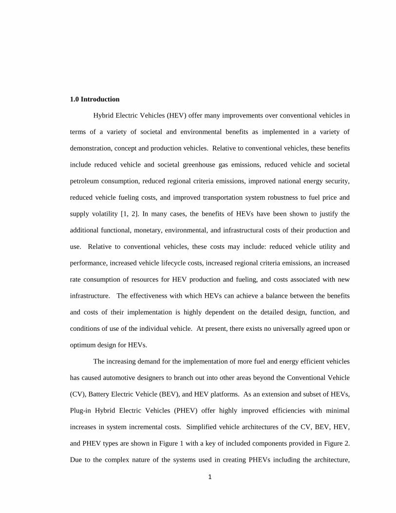
(CV), Battery Electric Vehicle (BEV), and HEV platforms. As an extension and subset of HEVs,
Plug-in Hybrid Electric Vehicles (PHEV) offer highly improved efficiencies with minimal
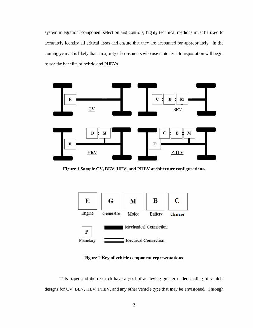
increases in system incremental costs. Simplified vehicle architectures of the CV, BEV, HEV,
and PHEV types are shown in Figure 1 with a key of included components provided in Figure 2.
Due to the complex nature of the systems used in creating PHEVs including the architecture,
2
system integration, component selection and controls, highly technical methods must be used to
accurately identify all critical areas and ensure that they are accounted for appropriately. In the
coming years it is likely that a majority of consumers who use motorized transportation will begin
to see the benefits of hybrid and PHEVs.
Figure 1 Sample CV, BEV, HEV, and PHEV architecture configurations.
Figure 2 Key of vehicle component representations.
This paper and the research have a goal of achieving greater understanding of vehicle
designs for CV, BEV, HEV, PHEV, and any other vehicle type that may be envisioned. Through
3
advanced computational techniques available such as modeling, simulation, and optimization
combined with an understanding of the underlying vehicular subsystems, conceptual analysis can
be performed on numerous vehicle architectures with reduced cost and efforts when compared
with conventional design and investigation methods. The models used in this study are created
through the use of defensible mathematical object-oriented modeling languages, tested in a
simulation specific domain, and optimized using multiple algorithms.
This introduction will provide an overview of the pathways that hybrid vehicle designers
follow, review of hybrid vehicle design techniques, the methods that are used to understand the
design process, and a description of the project that is presented in the remainder of this study.
These introductory sections supply a basis for the research done as well as a structure to assist in
organizing the complex design of advanced hybrid vehicles.
1.1 Hybrid Vehicle Design Pathways
The design of any complicated system (including HEVs) is complex, multi-objective, and
iterative. Further complicating the analysis of design is the details of commercial design
processes that are generally not published. Research into design methods is therefore necessarily
reductionist; the entire complexity of the design process cannot be described. Instead we must
understand and describe the inputs and outputs of the design process and its primary elements.
In the design process of any sufficiently complex system, including hybrid vehicles,
designers incorporate systems engineering techniques to aid in the organization and effectiveness
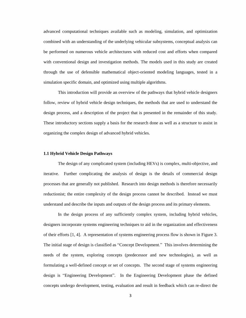
of their efforts [1, 4]. A representation of systems engineering process flow is shown in Figure 3.
The initial stage of design is classified as “Concept Development.” This involves determining the
needs of the system, exploring concepts (predecessor and new technologies), as well as
formulating a well-defined concept or set of concepts. The second stage of systems engineering
design is “Engineering Development”. In the Engineering Development phase the defined
concepts undergo development, testing, evaluation and result in feedback which can re-direct the
4
concept development phase or lead into the final Post Development phase. Although Figure 3 is
represented as a linear progression through the phases of design and development, in reality there
are many feedback loops and embedded iterations within and between phases. Although each of
the steps and phases will not be explored in depth through this research, they provide a
foundation for focusing on the complexities and available improvements that can exist in the
Concept Definition phase, as well as possibly in the Engineering Development phase.
Figure 3 Systems engineering design process
The Concept Development phase for hybrid vehicle design process applications can be
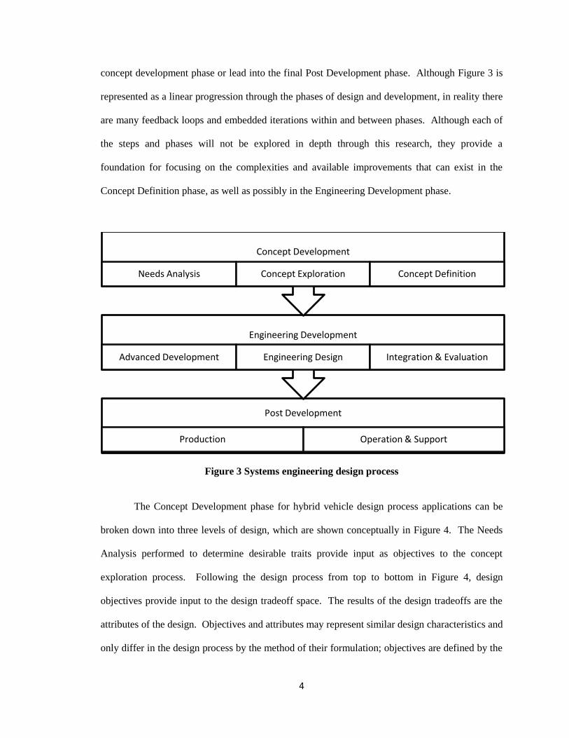
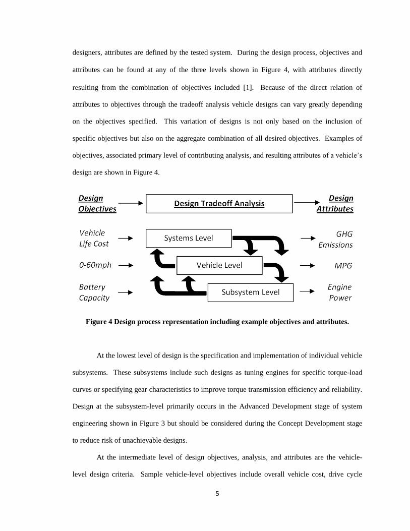
broken down into three levels of design, which are shown conceptually in Figure 4. The Needs
Analysis performed to determine desirable traits provide input as objectives to the concept
exploration process. Following the design process from top to bottom in Figure 4, design
objectives provide input to the design tradeoff space. The results of the design tradeoffs are the
attributes of the design. Objectives and attributes may represent similar design characteristics and
only differ in the design process by the method of their formulation; objectives are defined by the
Post Development
Production Operation & Support
Engineering Development
Advanced Development Engineering Design Integration & Evaluation
Concept Development
Needs Analysis Concept Exploration Concept Definition
5
designers, attributes are defined by the tested system. During the design process, objectives and
attributes can be found at any of the three levels shown in Figure 4, with attributes directly
resulting from the combination of objectives included [1]. Because of the direct relation of
attributes to objectives through the tradeoff analysis vehicle designs can vary greatly depending
on the objectives specified. This variation of designs is not only based on the inclusion of
specific objectives but also on the aggregate combination of all desired objectives. Examples of
objectives, associated primary level of contributing analysis, and resulting attributes of a vehicle’s
design are shown in Figure 4.
Figure 4 Design process representation including example objectives and attributes.
At the lowest level of design is the specification and implementation of individual vehicle
subsystems. These subsystems include such designs as tuning engines for specific torque-load
curves or specifying gear characteristics to improve torque transmission efficiency and reliability.
Design at the subsystem-level primarily occurs in the Advanced Development stage of system
engineering shown in Figure 3 but should be considered during the Concept Development stage
to reduce risk of unachievable designs.
At the intermediate level of design objectives, analysis, and attributes are the vehicle-
level design criteria. Sample vehicle-level objectives include overall vehicle cost, drive cycle
6
fuel economy, and driving range. Vehicle-level design attributes are determined solely by the
operation of the vehicle through its specified subsystem interactions. Vehicle-level design
attributes may include many of the conventional metrics of vehicle performance including 0-
60mph time, all-electric range (AER) or retail price which can each be determined from different
tests on a complete vehicle.
At the highest level are the objectives, analyses and attributes of system-level design.
System-level objectives, analyses and attributes describe the function of the vehicle as an element
in a larger system over which the vehicle designer may have only limited control. The systems to
be considered might be the transportation energy sector, the electric grid, an air quality
management district, or a transportation policy. System-level design objectives might include
goals for Greenhouse Gas emissions (GHG), petroleum displacement, or Corporate Average Fuel
Economy (CAFE) rating. Analyses to determine the attributes of a design relative to system-level
design objectives are generally outside of the scope of conventional vehicle engineering.
Understanding how information is exchanged between the levels and steps of the design
process is a foundation for creating prolific vehicle designs. Interactions between objectives,
tradeoffs and attributes can be observed between multiple levels. For example, a system-level
design objective such as net GHG emissions reduction may be transmitted to the vehicle level
contributing analysis as a requirement for high vehicle fuel economy. As another example,
particular battery chemistry may constrain the vehicle-level performance by increasing vehicle
weight relative to another design option. Although these examples provide sample interactions
between levels, all of the contributing objectives must be included for determination of trade-offs
and resulting attributes.
1.2 Review of Hybrid Vehicle Design
Using the classification of design objectives, contributions, and attributes proposed above
we can understand the vehicle design methods that have been proposed in literature on the basis
7
of the conceptual level of their design objectives. Each method has a set of primary design
objectives that are inputs to the design process. These objectives are the qualities that are to be
met by the resulting vehicle design. For this study the design objectives are divided into
subsystem-, vehicle-, and system-level categories.
The primary groups that have documented a vehicle design process with subsystem-level
design objectives are conversion and aftermarket modification companies. These companies have
the design objective of using an existing vehicle and making subsystem-level component
modifications or additions to achieve some improvement in a particular vehicle attribute.
Because these vehicles incorporate conversions and modifications, the designers have no control
over the other systems of the vehicle which have already been included. As an example of
subsystem-level design, PHEV conversion companies provide additional energy storage and
charging capabilities to preexisting HEVs. The desired resulting attributes of these modifications
include improved fuel economy and All Electric Range (AER). Due to the requirements of the
preexisting vehicle system used in subsystem-level design efforts, gains in attributes are
commonly limited.
Design processes with vehicle-level design objectives have been proposed by a number
of researchers and developers. A majority of historical examples of automotive designs have a
basis that resides at the vehicle-level. It is common for automotive manufactures to design
vehicles that can achieve specific attributes related to performance and or cost. For example, one
design attempt to achieve a certain mile per gallon (MPG) fuel consumption while reducing
production costs. Another designer may wish to primarily increase the acceleration performance
of the vehicle regardless of costs. Although many design efforts require an intensive amount of
subsystem-level component technology development and integration, the objectives for the end
product remain at the vehicle-level of design.
Design objectives that are posed at the system-level are less common. As standards for
emissions, CAFE, and regulations continue to increase, it becomes advantageous for designers to
8
begin exploring vehicle designs that can appropriately achieve a multitude of system-level
objectives. In order to effectively achieve system-level design objectives, the design process
must be directly formulated to incorporate the appropriate objective criteria and quantification of
resulting attributes. Applying vehicle- and subsystem-level design objectives solely have a
possibility in resulting in desirable system-level attributes, but will not be able to achieve their
full system-level attribute potential unless constrained so. As an example, a vehicle which is
designed to have low fuel consumption may also have low emissions, but this is not a direct
correlation. In fact, emissions may improve with other design considerations for an equivalent
mpg rating. Furthermore, the emissions objective may incorporate life-cycle factors, from which
vehicle-level specific values would be incapable to determine.
Overall, a majority of published design studies have design objectives that are posed at
the vehicle-level and below [1]. Upon review of design objectives from the literature, it becomes
evident that only through integrating component design, vehicle design, and systems design can
system-level design objectives be posed. Expressing design objectives at the system-level is
necessary to achieve the beneficial system-level vehicle attributes that have been proposed for
improved vehicle technology. To date, the system-level vehicle characteristics that have been
attributed to vehicles are not the result of a direct design process, they are byproducts of a
vehicle-level design process. In order to be able to improve the system-level attributes of
designed vehicles we must understand the connections between the design processes at the three
proposed levels.
1.3 Methods of Hybrid Vehicle Design
As previously discussed, Conceptual Design involves the interaction of the vehicle-level
objectives, analyses and attributes at the system- and subsystem-level objectives, analyses and
attributes of the system being designed. These connections have been studied in detail in the
existing literature on hybrid vehicles describing sustainability assessments, net GHG analyses,
9
grid impacts assessments and conceptual comparisons [1]. The methods used to carry out these
studies have included many systems engineering process such as mathematical modeling,
simulation, prototyping, subsystem testbed analysis, and retrofitting. Each of these design
methods offer tradeoffs, primarily between the cost of the method in terms of all resources and
the amount of information that is obtained from the method.
Within any chosen method of design, or in many cases a combination of all of the
methods, it is likely that multiple iterations must be performed before an acceptable design
solution is identified. Information is obtained as attributes resulting from the provided objectives
and chosen parameters which are fed back into the design process in an iterative looping process.
Commonly, additional efforts applied early in the design stages contribute to less overall cost as
resources tend to become exponentially more expensive as the design progresses along a timeline.
The incurred costs that can be realized at progressive phases of the design process include
increased risk of failing to meet deadlines, additional monetary costs for re-applied efforts to
previous analysis and a possibility of project failure. System design techniques of the past
focused on making well educated decisions about which components and configurations to
incorporate into a vehicle and then testing a demonstration version [5, 6]. Test results were
analyzed and quantified to provide feedback to the designers relating to possible needs for
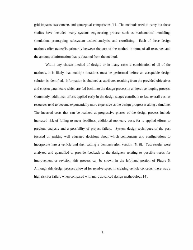
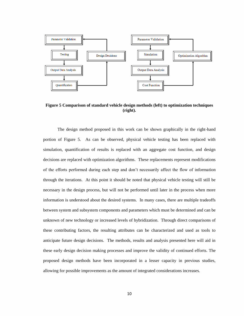
improvement or revision; this process can be shown in the left-hand portion of Figure 5.
Although this design process allowed for relative speed in creating vehicle concepts, there was a
high risk for failure when compared with more advanced design methodology [4].
10
Figure 5 Comparison of standard vehicle design methods (left) to optimization techniques
(right).
The design method proposed in this work can be shown graphically in the right-hand
portion of Figure 5. As can be observed, physical vehicle testing has been replaced with
simulation, quantification of results is replaced with an aggregate cost function, and design
decisions are replaced with optimization algorithms. These replacements represent modifications
of the efforts performed during each step and don’t necessarily affect the flow of information
through the iterations. At this point it should be noted that physical vehicle testing will still be
necessary in the design process, but will not be performed until later in the process when more
information is understood about the desired systems. In many cases, there are multiple tradeoffs
between system and subsystem components and parameters which must be determined and can be
unknown of new technology or increased levels of hybridization. Through direct comparisons of
these contributing factors, the resulting attributes can be characterized and used as tools to
anticipate future design decisions. The methods, results and analysis presented here will aid in
these early design decision making processes and improve the validity of continued efforts. The
proposed design methods have been incorporated in a lesser capacity in previous studies,
allowing for possible improvements as the amount of integrated considerations increases.
11
1.4 Project Description
This study makes initial optimizations and analysis of chosen vehicle architectures and
design objectives, results may be applied to future design. The approach and tools used within
the study will allow designers to more precisely apply system-level design objectives to vehicle-
level constraints and contributing trade-off analysis. There are multiple facets of development
which provide background for the work performed in this research project.
The first stage of the project development is to create a definition of the desirable aspects
of the design. Secondly, a defensible vehicle simulation must be constructed which is capable of
accommodating the necessary changes in design characteristics to achieve the final system
attributes. A feasible design space will be defined which aids in identifying the possible optimal
designs. Appropriate optimization algorithms will be selected based on previous works which
fulfill the objectives of the design and the vehicle simulation. An aggregate cost function is
defined to minimize the design’s life cycle cost. This is an example of a system-level design
objective. Finally, analysis will be performed to determine what choices should be made
concerning the design based on the results of the optimization study.
The results of the analysis will provide an example of improvements achieved through
the proposed techniques. Qualitative analysis will be performed specifically on the performance
of different optimization algorithms, the consistency of these algorithms to describe robustness,
characteristics of the design space, design sensitivity, and considerations that can be incorporated
into future design decisions.
By applying multiple exploration techniques with improved objectives and constraints, a
better understanding of each vehicle design can be achieved.
12
2.0 Methods
In order to help with an understanding of the systems that are in development, the
following sections (2.1-2.7) describe the main components of the research methods. This
description includes the programs used, an explanation of components represented within the
models, requirements of the simulations, and an exploration of the optimization techniques
implemented. Each of the before-mentioned aspects of the research contributes to an ability to
perform objective analysis of hybrid vehicle design.
2.1 Overview of Proposed Design Process
Design of hybrid vehicles is an extremely complex process which requires
comprehension of many different areas. Within the design there are many aspects of the system
which contribute to the overall vehicle design and optimization such as interactions between
electrical and mechanical mechanisms, controls, vehicle performance requirements, and
economic requirements. Systems engineering techniques allow us to logically categorize these
components and deal with them in a structured manner to ensure that all aspects are accounted for
properly as they have been defined. This involves considering the most important aspects of the
results attributes as well as the requirements of the systems under consideration to develop a
compilation of key components. This will be discussed further in Section 2.3 Developing Key
Components. The key components will then be combined in vehicle configurations which have
shown advantages. Optimization algorithms, discussed in section 2.6 Optimization Algorithms,
will be applied to see how these vehicles can be improved. The optimizations are limited to the
requirements that are presented for the system, accuracy of the models, physically achievable
components, and optimization methods chosen. As may be apparent from this statement, the
13
results can only be as good as the information supplied to the study. Consequentially, designers
must make a problem definition as accurate as possible, which brings up additional simulation
issues that are discussed in the following section 2.2.1 Requirements of the Model & Simulations.
As an exploratory example of the efficacy of using the methods presented through this
research the parameters that have been created to rank the vehicles characteristics are: overall
vehicle initial cost; vehicle fuel economy; ability of vehicle to operate on the EPA’s vehicle
testing cycles within a definable deviation as discussed in section 2.4 Drive Cycles; vehicle
acceleration characteristics; and fuel and energy costs. All of these can be combined into a
system-level design metric of vehicle-life cost to a consumer as described in section 2.7
Economic Analysis and Decision Making. These parameters help to define the manner in which
the models and simulations are created. Additional considerations are included such that
continued studies may be performed geared towards additional system-, vehicle-, and subsystem-
level design objectives. After the system and method have been sufficiently developed they
undergo testing in section 3.0 System Test and Evaluation. Finally, example results analysis and
conclusions are made in section 4.0 Results and Discussion and section 5.0 Conclusions
2.2 Simulation Tools
In the area of computer modeling and simulation there are many available programs and
modeling languages from which to choose. As general computational power increases with
technology each of these modeling tools improves as well with each of them offers their own
advantages and disadvantages. Some of the common simulation tools that are used in automotive
design include MatLab/Simulink, Advisor, Powertrain Systems Analysis Toolkit (PSAT), AVL,
Python, Dymola, Excel and many others [7, 8]. The primary areas of interest when dealing with
large amounts of modeling and simulation is the level of detail presented within the models and
the computational time necessary to run simulations. An inverse relation exists when adding
additional details to models requires more calculations and thus more computational time. In an
14
effort where hundreds or thousands of simulations may be necessary to satisfy an optimization,
even slight increases in simulation time can cause large increases in overall optimization efforts.
Other model and simulation requirements that are important include the ability of the program to
allow for modification of the components and parameters represented and accurate calculation of
the results attributes with appropriate precision.
The modeling language that has been chosen for use in this study is Modelica [9]. The
Modelica language is a free, open source language that is constantly developed and improved
through OpenModelica [10]. As a forward dynamic tool, defined by vehicle control which occurs
in a real-world stimulus-response manner, Modelica includes a solver developed to accurately
and quickly solve Differential Algebraic Equations (DAE’s). Hybrid vehicle models are
comprised of DAE’s which makes the OpenModelica modeling package a good fit for the
intended purpose [11]. Additionally, Modelica is organized as an object oriented language which
allows for class definition of components and systems which can be replicated, implemented, and
modified readily. The primary capabilities that are important inclusions in the model and
simulation to producing accurate results are included in the following sections.
2.2.1 Requirements of the Model & Simulations
As was mentioned in section 2.1 Overview of Proposed Design Process, the components
and parameters that have been defined aid in the creation of the vehicle simulations. One major
point where this is evident is the necessity for the model to represent each of the desired systems
accurately. Another pre-defined capability of the simulations is that they must have modifiable
and scalable components that can be updated throughout the optimization to represent the
different vehicle designs. There must be a capability of the simulated vehicle to follow some
defined course as accurately as possible to fulfill the drive cycle testing standards as well as the
acceleration and performance parameters. This list of necessities helps to form the general
structure of these simulations by requirement.
15
There is a design paradigm when the subject of simulation accuracy is discussed. The
more accurate a simulation is the more likely it is to be complex and costly in terms of necessary
computational power and time. Undefined limitations on a feasible amount of time that will be
allocated to running simulations and analysis cause limits to details in the models to only those
that are uniquely necessary. There is another concept of detailed design that must be considered
which is the relation of model complexity to output accuracy. It is likely that at some point in the
definition process a plateau will be reached in such a way that additional detail will add very little
accuracy. Additional discussion of the model outputs follows in section 2.2.4 Requirements of
Results.
2.2.2 Design Space Definition
When the vehicle simulations are applied to the optimization and analysis phases of the
process there must be an understanding by the designer as to whether the design is an absolute
optimal, a feasible optimal, a reproducible optimal or a combination of these classifications. The
differences between these designs are determined by the location of the design on a scale of
theoretical to physically available. The effects of the chosen design limitations are implemented
through a definition of the design space. The design space is a consideration that must be
determined by the designer to set constraints on all of the values which will be observed through
the design such as allowable costs, design variable values, performance, and etcetera.
When components and parameters are applied to the simulation there may be different
goals for the outcome. For instance, if a designer wants to see which components are the limiting
factors of the design they may produce a study that has constraints, observing which constraints
become active in optimal designs. By this it may be understood that an optimally chosen
component that is the furthest away from current technological state-of-the-art is likely a limiting
factor. In another case a designer may limit the design space to entirely obtainable components in
such a way that the vehicle would be immediately producible after completion of the study
16
without further development of technology; simply combining parts that are available on the
market.
It is foreseeable that definition of the design space within the obtainable domain can be
more complex because it requires the acquisition of information regarding the availability of
components, but it is also simpler in the same manner because the optimization has fewer choices
that it can make. The opposite can be said for theoretical design spaces because there are an
infinite number of design options but they are much simpler to define. Optimization variables
such as controller parameters fit into neither of these categories because they are not limited by
any real-world available technology thus having infinite options without creating an unbuildable
solution.
In addition to the classification of the design space based on feasibility or availability, it
is important to include design space constraints such that only physically producible products are
formed. For example, although there may not be a gear set available to the designer with an
optimal input/output ratio of exactly 2.5718 it is important to know that this is an optimal design
and may require further investigation to become acquirable. In contrast, if an ICE is not limited
in the design space to only producing positive power, a backwards running engine which
produces fuel instead of consuming it may enter the design. Through this specific example we
can see that although generalized design space definitions can be either constrained or
unconstrained base on the end design goal, certain realistic constraints that pertain to following
thermodynamic laws, etc. should be included.
2.2.3 Model Output Characteristics
The models used to simulate the vehicles within the study have been designed so that
quantifiable comparisons can be made between the resulting outputs. From these outputs,
represented through dynamic simulations on appropriate time scales; calculations of impacts on
cost, infrastructure, and societal impacts can be performed. Outputs of the simulations have been
17
defined within each of the models so that key attributes can be calculated from the resulting time-
series simulation data. A few of the key outputs that the simulations are capable of representing
include:
a. RCD (Driving range, Charge Depleting)
b. RCS (Driving Range, Charge Sustaining)
c. Fuel Consumption (and resulting emissions)
d. Performance (0-60, drive cycle profile maintenance, etc.)
e. Energy use (e.g. kWh/mi for each component)
f. System Efficiency (Input Energy/Energy required)
Some of the example uses of the outputs include using the charge sustaining range, charge
depleting range, and fuel consumption; to determine the vehicles approximate fuel cost per mile
as well as fuel costs per year. These values can then be added to the previously calculated vehicle
cost for an overall cost comparison. Vehicle performance can be evaluated to determine what the
driving characteristics of each vehicle are so that they may be evaluated equally. Additional
vehicle characteristics such as operational modes can also be observed and compared across
different vehicles and any cycle to determine, for example, if sizing constraints require an Internal
Combustion Engine (ICE) to turn on to maintain speed or fuel cell sizing inhibits charge
sustaining on demanding cycles. There are many ways in which the output of the simulations can
be used to calculate different operational aspects of the vehicle, because of this it is important to
include as the necessary outputs from each model and ensure that they are accurate. The manners
in which the simulation outputs are determined to be accurate are presented in the following
sections.
2.2.4 Requirements of Results
The results of the simulations for each vehicle model are the primary determinants of
continued design simulation and optimization. As such, they must be represented accurately and
18
in a sufficient manner. Depending on the specific value that is being observed in the simulation
there are different requirements [12].
One of the main distinctions for each calculated value in the model that creates
differences in the manner in which the system is put together (assuming that the value is desired),
is the rate at which the value should be calculated, also known as the time step. For example,
some variables in a hybrid vehicle model should be calculated using dynamically changing time
steps such as with compressible fluids, accelerations, and other highly dynamic interactions. The
simulation tool or language that is used in the model creation should be capable of either
adjusting to the changing time step needs of the simulation or operate at a constant time step that
is short enough to represent all of the systems functionality at an acceptable level. The second
option of using extremely small constant time steps is uncommon in many vehicle design efforts
due to the large amounts of computational effort and computational time necessary to complete
the common driving cycles. Other values such as controller inputs and outputs operate statically,
specifically in a controller output case where the time sampling rate is limited to physical output
frequencies of the controller used.
Another requirement of the results from both the simulations of the model and
optimizations is an ability to verify that the results are accurate. The two main factors affecting
this requirement are the equations which are used in the simulation and the parameter values that
are used by the governing equations to determine operational characteristics. The equations used
to represent the vehicles are briefly discussed in the following section 2.3 Developing Key
Components and the supporting validation. Parameter values used within the model to represent
component characteristics must be defensible in nature but are not required to be feasible as was
previously mentioned in section 2.2.2 Design Space Definition. Validation of parameter value
interactions within the model are verifiable through the system validation testing performed.
19
2.3 Developing Key Components
In order to achieve the desired outputs of the simulations, the components within the models
require at least a minimum amount of detail such that the calculations within the simulation are
accurate. Based on the vehicle architectures and operational methods chosen, the key
components in the vehicle models include a Battery, Fuel Cell (FC), Internal Combustion Engine
(ICE), Motor/Generator, Controller, Transmission, and Chassis/Vehicle Dynamics [13, 14]. Each
of these components has key aspects which must be addressed within the model. Scalable
parameter values are included within individual components so that any desirable size can be
represented accurately within the same operational type. Each of the components presented
within the model represent subsystem-level design criteria which contribute to the overall vehicle
and system-level design.
2.3.1 Chassis & Vehicle Dynamics
The vehicle’s chassis and performance dynamics portion of the model is intended to represent
the base structure of the vehicle (architecture) as well as the chassis glider elements. This
includes parameters such as final drive ratio, vehicle mass, rolling resistance, drag coefficient,
and wheel size so that vehicle acceleration dynamics can be calculated as the vehicle follows a
prescribed drive cycle. Torques and forces are transmitted between the vehicle’s environment
and all other components through the chassis.
2.3.1.1 Drivetrain Architecture
The PHEV drivetrain architecture subsystem consists of all of the powertrain components
that transmit power from the primary and secondary energy sources to the wheels of the vehicle.
The design of the drivetrain architecture subsystem includes design layout of the transmission,
motor/generators and final drive. The drivetrain architecture subsystem of the model is of
particular importance because it provides a general layout of the interactions that will exist
20
between other subsystems. Many vehicular design efforts in the HEV field have difficulties in
making comparisons across different architectures due to system complexities. Hybrid vehicle
drivetrain architectures can be classified into three main categories: series, parallel and power-
split.
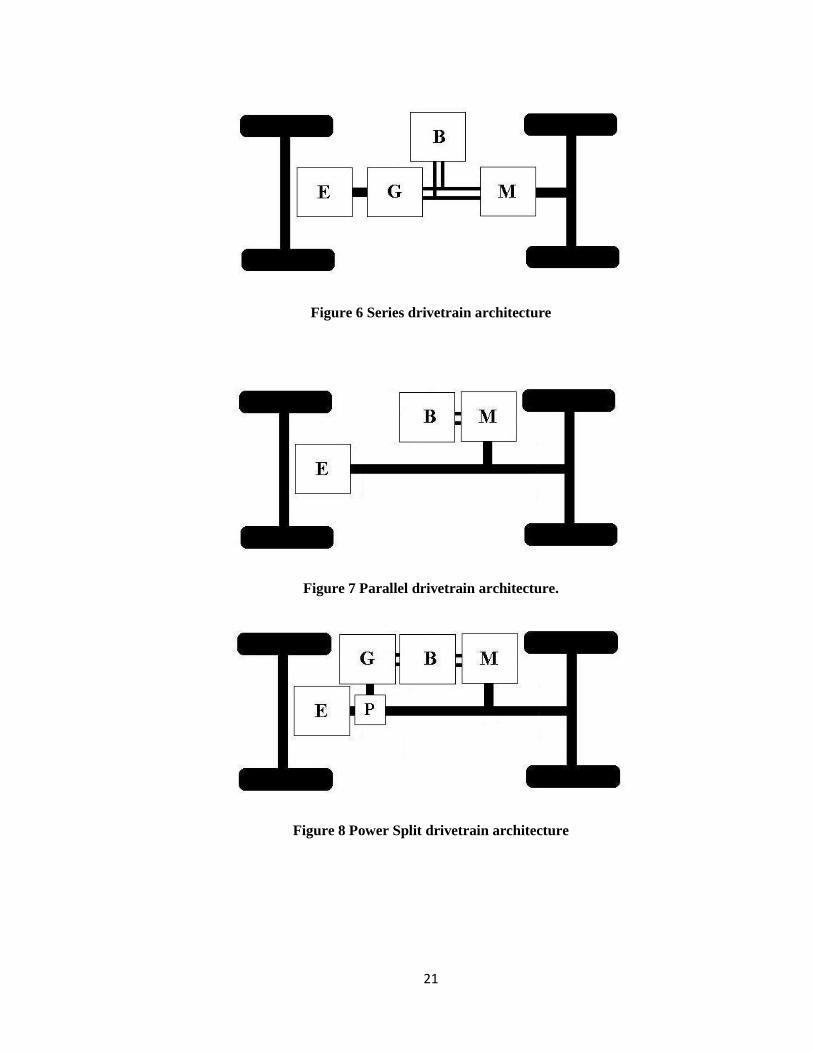
Series HEVs consist of a secondary power source, such as an internal combustion engine
or fuel cell, which is connected to a generator that charges the primary energy source (batteries).
The main subsystem components used in series HEVs can be seen in Figure 6. The batteries then
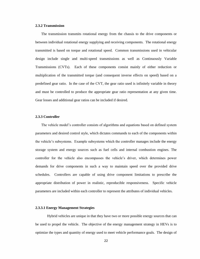
power a traction motor to drive the wheels. Parallel HEVs consist of an ICE which is
mechanically coupled with a traction motor. The coupling allows for torque addition between the
two units but creates other limiting factors. In most applications parallel systems are more
efficient and have fewer components than series HEVs (one engine and one motor as opposed to
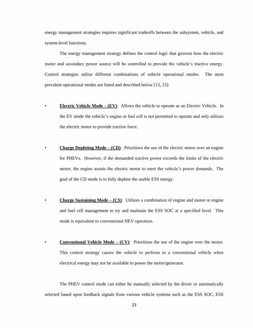
an engine, generator and motor in series systems) as shown in Figure 7. Power-split (or series-
parallel) HEVs are the most complicated of the three systems and combine the positive aspects of
both the series and parallel drivetrains. Power-split vehicles are most commonly composed of an
ICE coupled with a motor and generator through a speed coupling device such as a planetary
(epicyclic) gear set. This configuration offers high efficiency but with more complicated
powetrain design and control. An example of a power-split drivetrain is shown in Figure 8.
Each type of drivetrain architecture has costs and benefits, but to date there is no clear
optimum configuration for HEVs.
21
Figure 6 Series drivetrain architecture
Figure 7 Parallel drivetrain architecture.
Figure 8 Power Split drivetrain architecture
22
2.3.2 Transmission
The transmission transmits rotational energy from the chassis to the drive components or
between individual rotational energy supplying and receiving components. The rotational energy
transmitted is based on torque and rotational speed. Common transmissions used in vehicular
design include single and multi-speed transmissions as well as Continuously Variable
Transmissions (CVTs). Each of these components consist mainly of either reduction or
multiplication of the transmitted torque (and consequent inverse effects on speed) based on a
predefined gear ratio. In the case of the CVT, the gear ratio used is infinitely variable in theory
and must be controlled to produce the appropriate gear ratio representation at any given time.
Gear losses and additional gear ratios can be included if desired.
2.3.3 Controller
The vehicle model’s controller consists of algorithms and equations based on defined system
parameters and desired control style, which dictates commands to each of the components within
the vehicle’s subsystems. Example subsystems which the controller manages include the energy
storage system and energy sources such as fuel cells and internal combustion engines. The
controller for the vehicle also encompasses the vehicle’s driver, which determines power
demands for drive components in such a way to maintain speed over the provided drive
schedules. Controllers are capable of using drive component limitations to prescribe the
appropriate distribution of power in realistic, reproducible responsiveness. Specific vehicle
parameters are included within each controller to represent the attributes of individual vehicles.
2.3.3.1 Energy Management Strategies
Hybrid vehicles are unique in that they have two or more possible energy sources that can
be used to propel the vehicle. The objective of the energy management strategy in HEVs is to
optimize the types and quantity of energy used to meet vehicle performance goals. The design of
23
energy management strategies requires significant tradeoffs between the subsystem, vehicle, and
system-level functions.
The energy management strategy defines the control logic that governs how the electric
motor and secondary power source will be controlled to provide the vehicle’s tractive energy.
Control strategies utilize different combinations of vehicle operational modes. The most
prevalent operational modes are listed and described below [13, 15]:
• Electric Vehicle Mode – (EV): Allows the vehicle to operate as an Electric Vehicle. In
the EV mode the vehicle’s engine or fuel cell is not permitted to operate and only utilizes
the electric motor to provide tractive force.
• Charge Depleting Mode – (CD): Prioritizes the use of the electric motor over an engine
for PHEVs. However, if the demanded tractive power exceeds the limits of the electric
motor, the engine assists the electric motor to meet the vehicle’s power demands. The
goal of the CD mode is to fully deplete the usable ESS energy.
• Charge Sustaining Mode – (CS): Utilizes a combination of engine and motor or engine
and fuel cell management to try and maintain the ESS SOC at a specified level. This
mode is equivalent to conventional HEV operation.
• Conventional Vehicle Mode – (CV): Prioritizes the use of the engine over the motor.
This control strategy causes the vehicle to perform as a conventional vehicle when
electrical energy may not be available to power the motor/generator.
The PHEV control mode can either be manually selected by the driver or automatically
selected based upon feedback signals from various vehicle systems such as the ESS SOC, ESS
24
temperature, tractive power requirements, vehicle location, and expected trip length [16, 15, 17].
Vehicles can be classified based on the ways that the energy management strategy uses the
operational modes described above. Combinations of the operational strategies listed can create
blended mode vehicles which exhibit performance characteristics that meld the different vehicle
types.
2.3.4 Electric Motor Generator
The motor (EM) and generator (EG) are mechatronic components which convert electricity
(DC current) to torque and vice-versa. Component losses and subsequent energy usage are
calculated while limitations are determined by component parameter scaling and through
efficiency calculations based on both speed and torque demands provided by the vehicle
controller. In HEVs and PHEVs, the EM can be used for the primary tractive efforts so that
electrical energy stored is used instead of secondary fuel sources for propulsion. The different
types of electric motors and generators can all be characterized by power limitations, torque
curves and efficiency maps which are utilized in the simulation models.
2.3.5 Fuel Cell
Fuel cells can be utilized as an energy source in which hydrogen (most common) or other
hydrocarbons can be used in conversion processes to produce electricity. Since the fuel cell
performs similar to an engine combined with a generator; similar inputs and outputs must be
present. The fuel cell component model has been represented in both a static and dynamic version
and has been verified both against one another and functioning fuel cell data. The application
which is more relevant for optimizations is the static model which can reduce computational costs
over the dynamic model while still accurately portraying the most important characteristics. The
static fuel cell model consists of fuel cell polarization and efficiency curves for a single cell from
the California Air Resource Board (ARB) [18] and has been verified by dynamic simulations as
25
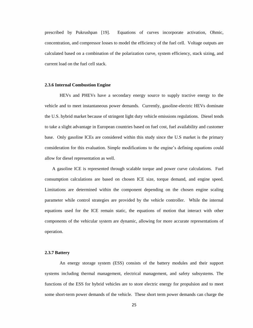
prescribed by Pukrushpan [19]. Equations of curves incorporate activation, Ohmic,
concentration, and compressor losses to model the efficiency of the fuel cell. Voltage outputs are
calculated based on a combination of the polarization curve, system efficiency, stack sizing, and
current load on the fuel cell stack.
2.3.6 Internal Combustion Engine
HEVs and PHEVs have a secondary energy source to supply tractive energy to the
vehicle and to meet instantaneous power demands. Currently, gasoline-electric HEVs dominate
the U.S. hybrid market because of stringent light duty vehicle emissions regulations. Diesel tends
to take a slight advantage in European countries based on fuel cost, fuel availability and customer
base. Only gasoline ICEs are considered within this study since the U.S market is the primary
consideration for this evaluation. Simple modifications to the engine’s defining equations could
allow for diesel representation as well.
A gasoline ICE is represented through scalable torque and power curve calculations. Fuel
consumption calculations are based on chosen ICE size, torque demand, and engine speed.
Limitations are determined within the component depending on the chosen engine scaling
parameter while control strategies are provided by the vehicle controller. While the internal
equations used for the ICE remain static, the equations of motion that interact with other
components of the vehicular system are dynamic, allowing for more accurate representations of
operation.
2.3.7 Battery
An energy storage system (ESS) consists of the battery modules and their support
systems including thermal management, electrical management, and safety subsystems. The
functions of the ESS for hybrid vehicles are to store electric energy for propulsion and to meet
some short-term power demands of the vehicle. These short term power demands can charge the
26
ESS in the case of regenerative braking, or they can discharge the ESS, in the case of vehicle
accelerations. The batteries must perform these functions at a variety of states of charge (SOC).
The consensus of recent meetings and publications on battery systems for hybrid vehicles is
that Lithium Ion (Li Ion) battery systems will be the battery system of choice for near and long
term applications. Other technologies, including lead-acid and nickel-metal hydride will not meet
the performance and cost points required for mass market vehicle applications [18]. Battery
characteristics for simulation are calculated using scaling based on individual battery cells.
Battery internal resistance, open circuit voltage, power density and energy density are input
parameters which allow for output voltage to be calculated based on battery state of charge
(SOC). Battery power availability information for charging and discharging is transmitted to the
vehicle controller as well as to the electric drive components for propulsion and to accessories for
miscellaneous use.
2.3.8 Miscellaneous Power Electronics
Vehicles contain a variety of power electronics whose increased use affects the
performance, particular when used with hybrid electric or battery electric vehicles. A few of the
miscellaneous power electronics represented through the vehicle models include air conditioning,
DC-DC converter, ESS and ICE thermal management systems, and cabin heating. As vehicle
technology continues to advance, many manufacturers are utilizing electronically powered
accessories which are more efficient and can be used in a larger variety of conditions. The
primary constraint affecting most of these systems is that in conventional vehicles many
components are belt powered from the engine. In hybrid vehicles the ICE may not be operating
at all times, but the power electronics and thermal conditioning systems must be able to perform
their specified tasks. In hybrid vehicle models, the use of additional power electrons can be
modeled through both their function and simply as additional electrical loads. Ambient
27
temperature effects are not represented in the considered simulations and testing that relies on
thermal effects are explained in the following Drive Cycles section.
2.4 Drive Cycles
In the work of modeling and simulating systems it is helpful to use standardized parameters
to improve validation techniques and justification. The simulations of vehicle models that have
been created through the research presented in this paper must have consistent simulation-domain
time-dependent operational profile requirements that can be analyzed, compared, and evaluated.
In vehicle simulation efforts it is common practice to subject the models to time sampled vehicle
velocity profiles known as drive cycles [2]. The driving cycles examined in the following
sections were initially created as testing metrics for physical vehicles and are appropriate for
application to analytical models for performance comparison between computational vehicle
representations and their production counterparts. The drive cycles that have initially been
selected as candidates for use in the vehicle simulations include the UDDS (Urban Dynamometer
Driving Schedule, note FTP-72, and FUDS), the FHDS (Federal Highway Driving Schedule, also
known as HWFET and HFET), US06 (also known as a SFTP; Supplemental Federal Test
Procedure), the SC03 (a SFTP of the FTP-75), and other FTP (Federal Test Procedure). The
main four cycles under consideration (UDDS, FHDS, US06 and SC03) can be seen in Figure 9,
Figure 11, Figure 12, and Figure 13. The figures of the cycles represent the time-dependent
velocity profiles. These cycles were chosen because of their ability to determine vehicular
performance in a variety of driving scenarios, visible from the different styles and magnitudes of
the driving profiles. The United States Environmental Protection Agency (EPA) and many other
testing and regulatory divisions have used many of these cycles for close to 30 years as standards
which are continually updated to match the current trends in driving profiles and vehicle
component capabilities [20].
28
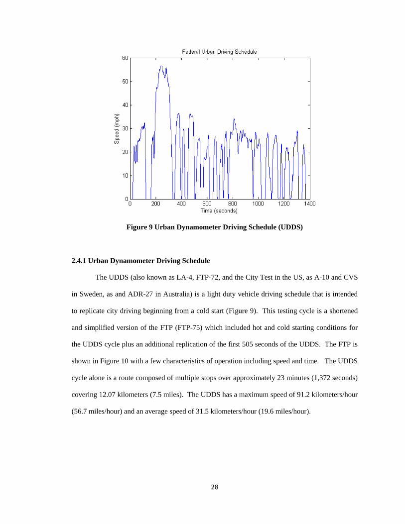
Figure 9 Urban Dynamometer Driving Schedule (UDDS)
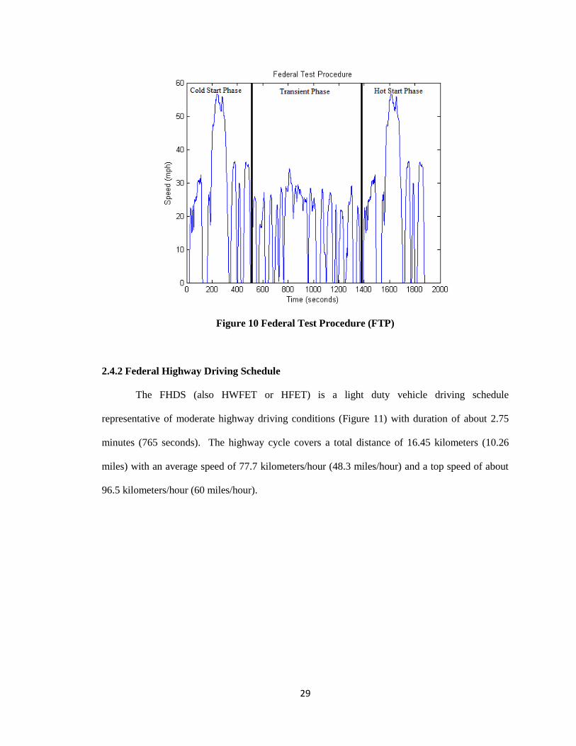
2.4.1 Urban Dynamometer Driving Schedule
The UDDS (also known as LA-4, FTP-72, and the City Test in the US, as A-10 and CVS
in Sweden, as and ADR-27 in Australia) is a light duty vehicle driving schedule that is intended
to replicate city driving beginning from a cold start (Figure 9). This testing cycle is a shortened
and simplified version of the FTP (FTP-75) which included hot and cold starting conditions for
the UDDS cycle plus an additional replication of the first 505 seconds of the UDDS. The FTP is
shown in Figure 10 with a few characteristics of operation including speed and time. The UDDS
cycle alone is a route composed of multiple stops over approximately 23 minutes (1,372 seconds)
covering 12.07 kilometers (7.5 miles). The UDDS has a maximum speed of 91.2 kilometers/hour
(56.7 miles/hour) and an average speed of 31.5 kilometers/hour (19.6 miles/hour).
29
Figure 10 Federal Test Procedure (FTP)
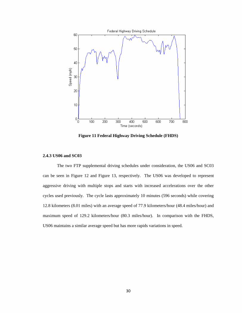
2.4.2 Federal Highway Driving Schedule
The FHDS (also HWFET or HFET) is a light duty vehicle driving schedule
representative of moderate highway driving conditions (Figure 11) with duration of about 2.75
minutes (765 seconds). The highway cycle covers a total distance of 16.45 kilometers (10.26
miles) with an average speed of 77.7 kilometers/hour (48.3 miles/hour) and a top speed of about
96.5 kilometers/hour (60 miles/hour).
30
Figure 11 Federal Highway Driving Schedule (FHDS)
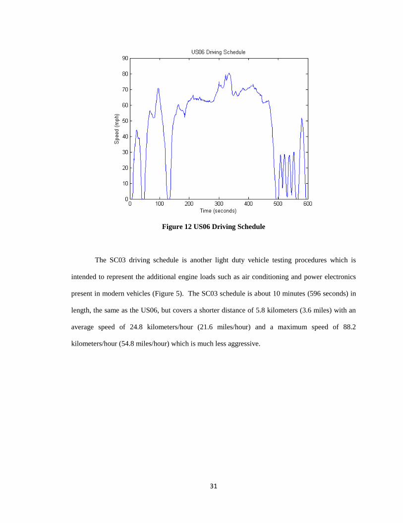
2.4.3 US06 and SC03
The two FTP supplemental driving schedules under consideration, the US06 and SC03
can be seen in Figure 12 and Figure 13, respectively. The US06 was developed to represent
aggressive driving with multiple stops and starts with increased accelerations over the other
cycles used previously. The cycle lasts approximately 10 minutes (596 seconds) while covering
12.8 kilometers (8.01 miles) with an average speed of 77.9 kilometers/hour (48.4 miles/hour) and
maximum speed of 129.2 kilometers/hour (80.3 miles/hour). In comparison with the FHDS,
US06 maintains a similar average speed but has more rapids variations in speed.
31
Figure 12 US06 Driving Schedule
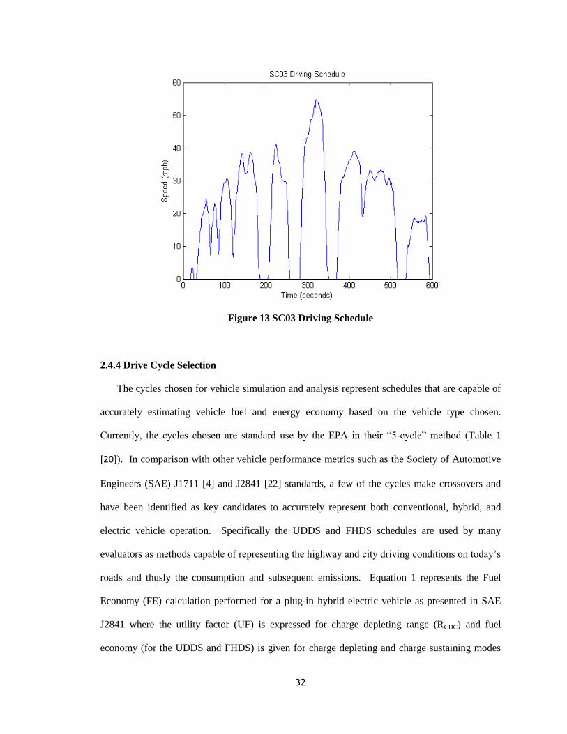
The SC03 driving schedule is another light duty vehicle testing procedures which is
intended to represent the additional engine loads such as air conditioning and power electronics
present in modern vehicles (Figure 5). The SC03 schedule is about 10 minutes (596 seconds) in
length, the same as the US06, but covers a shorter distance of 5.8 kilometers (3.6 miles) with an
average speed of 24.8 kilometers/hour (21.6 miles/hour) and a maximum speed of 88.2
kilometers/hour (54.8 miles/hour) which is much less aggressive.
32
Figure 13 SC03 Driving Schedule
2.4.4 Drive Cycle Selection
The cycles chosen for vehicle simulation and analysis represent schedules that are capable of
accurately estimating vehicle fuel and energy economy based on the vehicle type chosen.
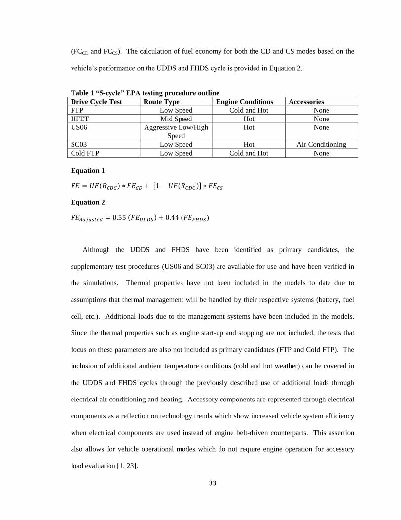
Currently, the cycles chosen are standard use by the EPA in their “5-cycle” method (Table 1
[20]). In comparison with other vehicle performance metrics such as the Society of Automotive
Engineers (SAE) J1711 [4] and J2841 [22] standards, a few of the cycles make crossovers and
have been identified as key candidates to accurately represent both conventional, hybrid, and
electric vehicle operation. Specifically the UDDS and FHDS schedules are used by many
evaluators as methods capable of representing the highway and city driving conditions on today’s
roads and thusly the consumption and subsequent emissions. Equation 1 represents the Fuel
Economy (FE) calculation performed for a plug-in hybrid electric vehicle as presented in SAE
J2841 where the utility factor (UF) is expressed for charge depleting range (RCDC) and fuel
economy (for the UDDS and FHDS) is given for charge depleting and charge sustaining modes
33
(FCCD and FCCS). The calculation of fuel economy for both the CD and CS modes based on the
vehicle’s performance on the UDDS and FHDS cycle is provided in Equation 2.
Table 1 “5-cycle” EPA testing procedure outline
Drive Cycle Test Route Type Engine Conditions Accessories
FTP Low Speed Cold and Hot None
HFET Mid Speed Hot None
US06 Aggressive Low/High
Speed
Hot None
SC03 Low Speed Hot Air Conditioning
Cold FTP Low Speed Cold and Hot None
Equation 1
Equation 2
Although the UDDS and FHDS have been identified as primary candidates, the
supplementary test procedures (US06 and SC03) are available for use and have been verified in
the simulations. Thermal properties have not been included in the models to date due to
assumptions that thermal management will be handled by their respective systems (battery, fuel
cell, etc.). Additional loads due to the management systems have been included in the models.
Since the thermal properties such as engine start-up and stopping are not included, the tests that
focus on these parameters are also not included as primary candidates (FTP and Cold FTP). The
inclusion of additional ambient temperature conditions (cold and hot weather) can be covered in
the UDDS and FHDS cycles through the previously described use of additional loads through
electrical air conditioning and heating. Accessory components are represented through electrical
components as a reflection on technology trends which show increased vehicle system efficiency
when electrical components are used instead of engine belt-driven counterparts. This assertion
also allows for vehicle operational modes which do not require engine operation for accessory
load evaluation [1, 23].
34
Tests performed on vehicles with an ICE are considered to be “hot start” tests wherein
operating temperatures have reached steady-state conditions. Further extensions of the research
presented in this paper to include thermal effects on fuel consumption and emissions have been
considered but are deemed insignificant for preliminary presentations of method utility.
An acceleration drive cycle has also been included in the simulations but was not explored
through the cycle presentations as it only consists of a step-input which requests that the vehicle
operate at its highest performance capacity. This cycle has been used in vehicle simulation to
evaluate parameters such as 0-60mph, maximum acceleration rate achieved, 40-60mph passing
time, and maximum vehicle operating speed.
The drive cycles that have been presented and selected for use in the vehicle simulations
represent a comprehensive set of test procedures which can be used to evaluate vehicle
operational performance. The cycles that have been defined are used commonly for physical
vehicle testing purposes and allow for comparisons between simulated and production vehicles.
The UDDS, FHDS, and acceleration drive cycles will be used primarily in following sections for
system testing, validation, and analysis.
2.6 Optimization Algorithms
Optimization as a technique is very general in its use of achieving a most desirable
solution defined within the parameters of the algorithm. Within the umbrella of optimization
there are many individual techniques and caveats that must be understood to improve the
optimality of the optimization. One reason is that different algorithms search for different trends
within data and have different techniques for finding solutions. Also, there are parameter values
that define the operating conditions of each of the algorithms differently and affect their
performance. The principles behind this dilemma are what lead systems engineers working with
optimizations to examine multiple optimization algorithms to understand both the techniques and
goals of each [24].
35
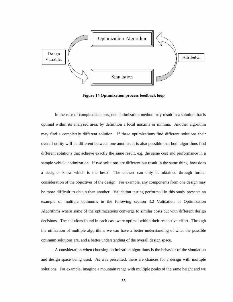
Figure 14 Optimization process feedback loop
In the case of complex data sets, one optimization method may result in a solution that is
optimal within its analyzed area, by definition a local maxima or minima. Another algorithm
may find a completely different solution. If these optimizations find different solutions their
overall utility will be different between one another. It is also possible that both algorithms find
different solutions that achieve exactly the same result, e.g. the same cost and performance in a
sample vehicle optimization. If two solutions are different but result in the same thing, how does
a designer know which is the best? The answer can only be obtained through further
consideration of the objectives of the design. For example, any components from one design may
be more difficult to obtain than another. Validation testing performed in this study presents an
example of multiple optimums in the following section 3.2 Validation of Optimization
Algorithms where some of the optimizations converge to similar costs but with different design
decisions. The solutions found in each case were optimal within their respective effort. Through
the utilization of multiple algorithms we can have a better understanding of what the possible
optimum solutions are, and a better understanding of the overall design space.
A consideration when choosing optimization algorithms is the behavior of the simulation
and design space being used. As was presented, there are chances for a design with multiple
solutions. For example, imagine a mountain range with multiple peaks of the same height and we
36
are trying to find the highest point in the region. Some design objectives may result in a single
optimal solution. While a technique that simply observes the slope of the land may find a single
peak quicker, a technique that takes random sampling over the whole area may find a better
solution, albeit slower. These differentiations in technique describe some of the underlying
principles in the many optimization techniques where the slope of the mountain may relate more
directly to the slope of a cost function peaking at an optimal value. Many other options such as
discontinuities, “flat” areas in objective functions, and seemingly random distributions cause
complexities in optimizations and increase the need for both an understanding of the design space
and the different algorithms that should be utilized. The algorithms used within this study which
will be explored in the following sections including Divided Rectangles (DIRECT), Genetic
Algorithm (GA), Particle Swarm Optimization (PSO), and Simulated Annealing (SA) [40, 25].
Between these algorithms different methods of optimization are used. All of the methods
explored are global optimizers with derivative-free algorithms (no gradient or slope as the
previous example mentioned). Global searches refer to an ability to evaluate design variables
throughout the design space. Due to specified design criteria, global searches may or may not be
limited to specified design spaces, as presented in section 2.2.2 Design Space Definition, in
which case the global search can occur at any point within the design space. All of the algorithms
used are heuristic, meaning they incorporate methods which “learn” and make increasingly
improved design decisions as the optimization search progresses. The DIRECT optimization
algorithm uses a deterministic method which is mathematically consistent whereas SA, GA and
PSO all use stochastic methods. Stochastic algorithms incorporate random search methods
whereas deterministic algorithms are structured. Further explanation of the differences and
unique methods of optimization for each of the algorithms is included in the following sections.
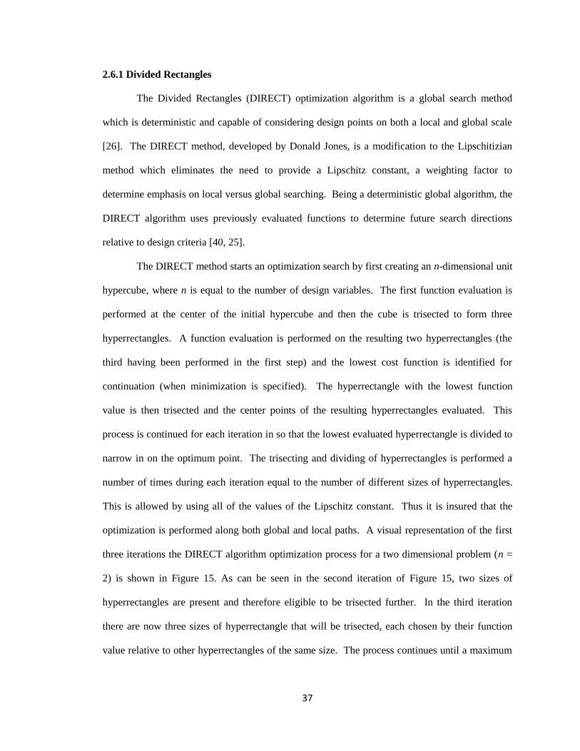
37
2.6.1 Divided Rectangles
The Divided Rectangles (DIRECT) optimization algorithm is a global search method
which is deterministic and capable of considering design points on both a local and global scale
[26]. The DIRECT method, developed by Donald Jones, is a modification to the Lipschitizian
method which eliminates the need to provide a Lipschitz constant, a weighting factor to
determine emphasis on local versus global searching. Being a deterministic global algorithm, the
DIRECT algorithm uses previously evaluated functions to determine future search directions
relative to design criteria [40, 25].
The DIRECT method starts an optimization search by first creating an n-dimensional unit
hypercube, where n is equal to the number of design variables. The first function evaluation is
performed at the center of the initial hypercube and then the cube is trisected to form three
hyperrectangles. A function evaluation is performed on the resulting two hyperrectangles (the
third having been performed in the first step) and the lowest cost function is identified for
continuation (when minimization is specified). The hyperrectangle with the lowest function
value is then trisected and the center points of the resulting hyperrectangles evaluated. This
process is continued for each iteration in so that the lowest evaluated hyperrectangle is divided to
narrow in on the optimum point. The trisecting and dividing of hyperrectangles is performed a
number of times during each iteration equal to the number of different sizes of hyperrectangles.
This is allowed by using all of the values of the Lipschitz constant. Thus it is insured that the
optimization is performed along both global and local paths. A visual representation of the first
three iterations the DIRECT algorithm optimization process for a two dimensional problem (n =
2) is shown in Figure 15. As can be seen in the second iteration of Figure 15, two sizes of
hyperrectangles are present and therefore eligible to be trisected further. In the third iteration
there are now three sizes of hyperrectangle that will be trisected, each chosen by their function
value relative to other hyperrectangles of the same size. The process continues until a maximum
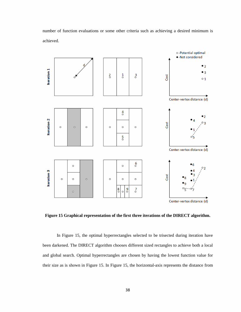
38
number of function evaluations or some other criteria such as achieving a desired minimum is
achieved.
Figure 15 Graphical representation of the first three iterations of the DIRECT algorithm.
In Figure 15, the optimal hyperrectangles selected to be trisected during iteration have
been darkened. The DIRECT algorithm chooses different sized rectangles to achieve both a local
and global search. Optimal hyperrectangles are chosen by having the lowest function value for
their size as is shown in Figure 15. In Figure 15, the horizontal-axis represents the distance from
39
the center to the vertex of each hyperrectangle and the vertical-axis represents objective function
value at the center point of the corresponding hyperrectangle.
2.6.2 Genetic Algorithm
The Genetic Algorithm (GA) used for optimization is a stochastic global search algorithm
based on Darwin’s concept of natural selection [40, 25]. The algorithm behaves as an
evolutionary population in which the fittest members survive and replicate and weak members are
eliminated. This process applies each member of the population as a set of design parameters
which are generated and the fitness of each of these members is determined by the function
evaluation of those design parameters for that member. Within the algorithm several natural
processes occur including mutation, drift, natural selection and crossovers between the members
as new generations are created. In Equation 3 a possible combination of genetic algorithm
parameters is provided where represents the next multi-dimensional design point,
represents the previous design, is other good designs found,
represents poor designs found
with a random probability of being included, drift represents minute adjustments, and mutation
allows for changes in magnitude and direction to the new design point. Design points with good
function values or fitness are used to produce further design points. Design points with poor
function values are excluded, allowing for the best design parameter points to be identified and
used.
Equation 3
The process begins with a set of initial design parameter points, or an initial population,
which is then evaluated. Based on the function values of each of the members of the population
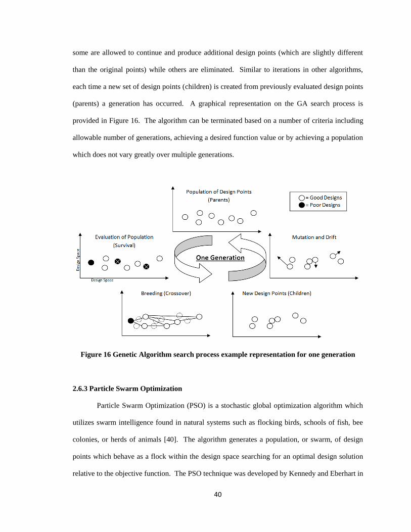
40
some are allowed to continue and produce additional design points (which are slightly different
than the original points) while others are eliminated. Similar to iterations in other algorithms,
each time a new set of design points (children) is created from previously evaluated design points
(parents) a generation has occurred. A graphical representation on the GA search process is
provided in Figure 16. The algorithm can be terminated based on a number of criteria including
allowable number of generations, achieving a desired function value or by achieving a population
which does not vary greatly over multiple generations.
Figure 16 Genetic Algorithm search process example representation for one generation
2.6.3 Particle Swarm Optimization
Particle Swarm Optimization (PSO) is a stochastic global optimization algorithm which
utilizes swarm intelligence found in natural systems such as flocking birds, schools of fish, bee
colonies, or herds of animals [40]. The algorithm generates a population, or swarm, of design
points which behave as a flock within the design space searching for an optimal design solution
relative to the objective function. The PSO technique was developed by Kennedy and Eberhart in
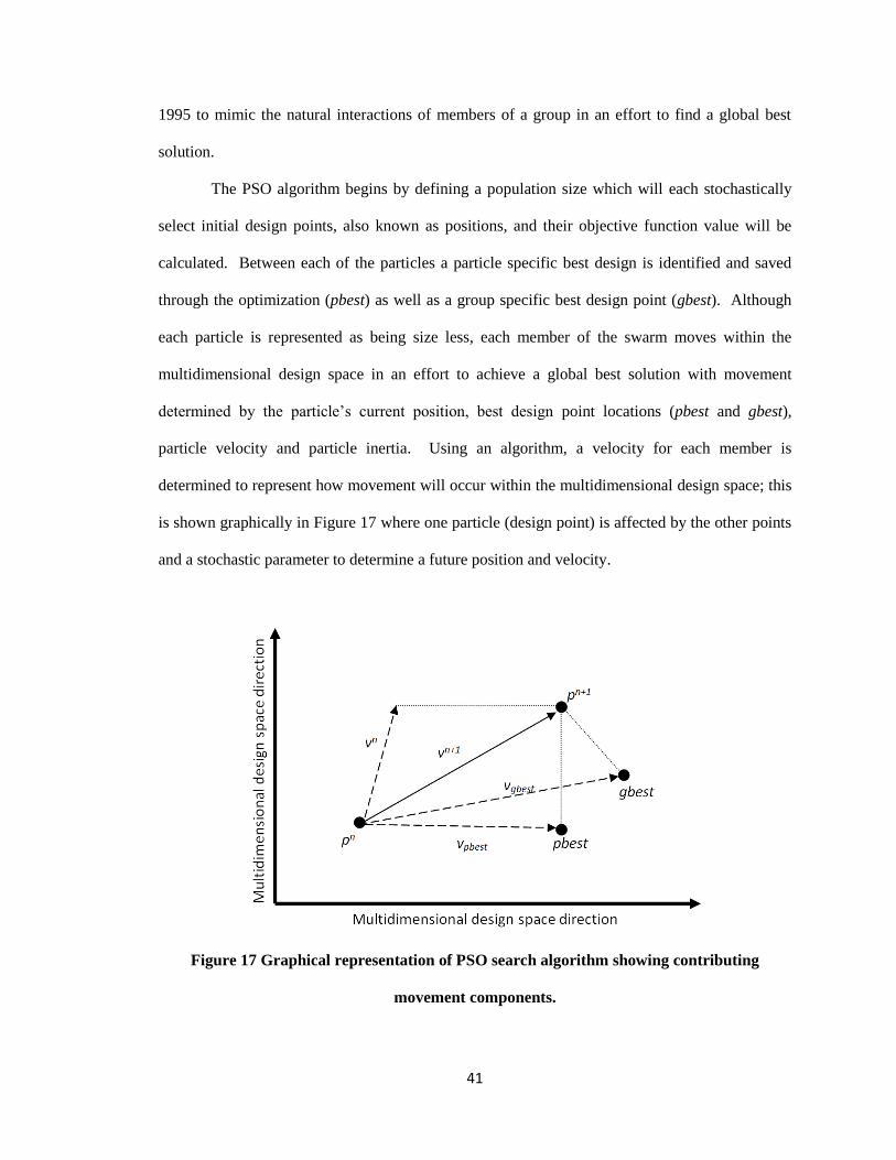
41
1995 to mimic the natural interactions of members of a group in an effort to find a global best
solution.
The PSO algorithm begins by defining a population size which will each stochastically
select initial design points, also known as positions, and their objective function value will be
calculated. Between each of the particles a particle specific best design is identified and saved
through the optimization (pbest) as well as a group specific best design point (gbest). Although
each particle is represented as being size less, each member of the swarm moves within the
multidimensional design space in an effort to achieve a global best solution with movement
determined by the particle’s current position, best design point locations (pbest and gbest),
particle velocity and particle inertia. Using an algorithm, a velocity for each member is
determined to represent how movement will occur within the multidimensional design space; this
is shown graphically in Figure 17 where one particle (design point) is affected by the other points
and a stochastic parameter to determine a future position and velocity.
Figure 17 Graphical representation of PSO search algorithm showing contributing
movement components.
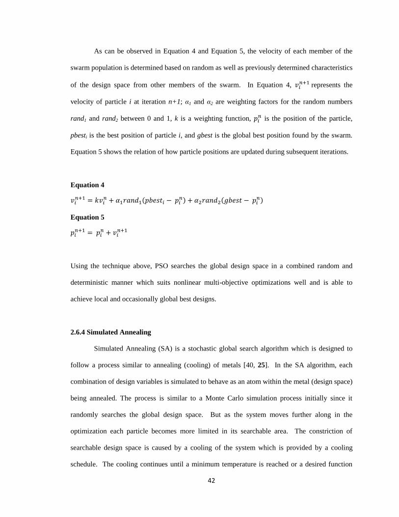
42
As can be observed in Equation 4 and Equation 5, the velocity of each member of the
swarm population is determined based on random as well as previously determined characteristics
of the design space from other members of the swarm. In Equation 4, represents the
velocity of particle i at iteration n+1; α1 and α2 are weighting factors for the random numbers
rand1 and rand2 between 0 and 1, k is a weighting function, is the position of the particle,
pbesti is the best position of particle i, and gbest is the global best position found by the swarm.
Equation 5 shows the relation of how particle positions are updated during subsequent iterations.
Equation 4
Equation 5
Using the technique above, PSO searches the global design space in a combined random and
deterministic manner which suits nonlinear multi-objective optimizations well and is able to
achieve local and occasionally global best designs.
2.6.4 Simulated Annealing
Simulated Annealing (SA) is a stochastic global search algorithm which is designed to
follow a process similar to annealing (cooling) of metals [40, 25]. In the SA algorithm, each
combination of design variables is simulated to behave as an atom within the metal (design space)
being annealed. The process is similar to a Monte Carlo simulation process initially since it
randomly searches the global design space. But as the system moves further along in the
optimization each particle becomes more limited in its searchable area. The constriction of
searchable design space is caused by a cooling of the system which is provided by a cooling
schedule. The cooling continues until a minimum temperature is reached or a desired function
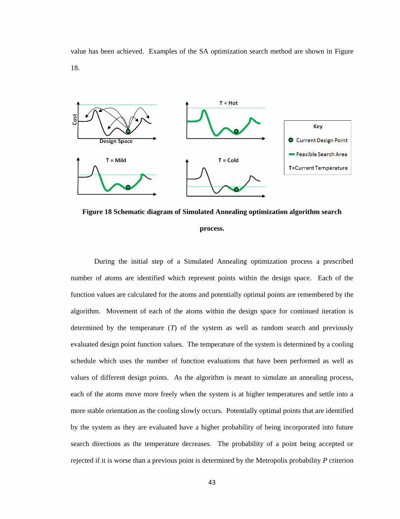
43
value has been achieved. Examples of the SA optimization search method are shown in Figure
18.
Figure 18 Schematic diagram of Simulated Annealing optimization algorithm search
process.
During the initial step of a Simulated Annealing optimization process a prescribed
number of atoms are identified which represent points within the design space. Each of the
function values are calculated for the atoms and potentially optimal points are remembered by the
algorithm. Movement of each of the atoms within the design space for continued iteration is
determined by the temperature (T) of the system as well as random search and previously
evaluated design point function values. The temperature of the system is determined by a cooling
schedule which uses the number of function evaluations that have been performed as well as
values of different design points. As the algorithm is meant to simulate an annealing process,
each of the atoms move more freely when the system is at higher temperatures and settle into a
more stable orientation as the cooling slowly occurs. Potentially optimal points that are identified
by the system as they are evaluated have a higher probability of being incorporated into future
search directions as the temperature decreases. The probability of a point being accepted or
rejected if it is worse than a previous point is determined by the Metropolis probability P criterion
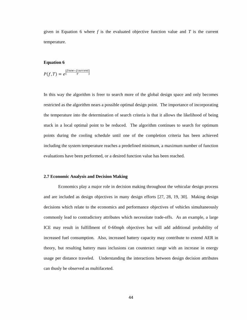
44
given in Equation 6 where f is the evaluated objective function value and T is the current
temperature.
Equation 6
In this way the algorithm is freer to search more of the global design space and only becomes
restricted as the algorithm nears a possible optimal design point. The importance of incorporating
the temperature into the determination of search criteria is that it allows the likelihood of being
stuck in a local optimal point to be reduced. The algorithm continues to search for optimum
points during the cooling schedule until one of the completion criteria has been achieved
including the system temperature reaches a predefined minimum, a maximum number of function
evaluations have been performed, or a desired function value has been reached.
2.7 Economic Analysis and Decision Making
Economics play a major role in decision making throughout the vehicular design process
and are included as design objectives in many design efforts [27, 28, 19, 30]. Making design
decisions which relate to the economics and performance objectives of vehicles simultaneously
commonly lead to contradictory attributes which necessitate trade-offs. As an example, a large
ICE may result in fulfillment of 0-60mph objectives but will add additional probability of
increased fuel consumption. Also, increased battery capacity may contribute to extend AER in
theory, but resulting battery mass inclusions can counteract range with an increase in energy
usage per distance traveled. Understanding the interactions between design decision attributes
can thusly be observed as multifaceted.
45
To overcome the issue of multiple objectives, optimization parameters will be integrated
in the system through aggregate cost functions to find solutions that are optimal in relation to all
of the included objectives. Cost models which approximate system components in multiple
respects contribute to the ability of this work to perform objective quantifications.
As an exploratory example of the system design process which is presented in this
research, designs which exhibit specific trade-offs between vehicle-level cost and performance
will be shown as a system-level design objective. The system-level design objective explored
will be a relative vehicle-life cost to one owner representing the majority of incurred costs. The
two main aspects of cost that must be considered are the initial cost to the consumer and the life
cycle costs such as fueling and charging. More specifics are presented in the following sections
regarding the specific algorithms and cost functions that will be implemented to fulfill the
system-level design objective.
In review, the optimization algorithms used are mathematical set of commands that
provide a series of design variable inputs to the modeling simulation. By observing the results of
those simulations subsequent design variables can be produced until an optimal is found. This
process is shown conceptually in Figure 5 and Figure 14. A cost function is a mathematical
equation written to combine the output values of attributes from the simulations into quantifiable
information that can be compared appropriately. Cost functions, also known as objective
functions, define measures of the system being analyzed which will be critical in the resulting
solution. For this study functions analyzed will include cost and performance measures.
Within the cost function and optimization algorithm, attributes of designs must be
verified through the use of appropriate design parameters as discussed in section 2.2.2 Design
Space Definition. As part of this, state-of-the-art cost, mass, and performance data have been
acquired for critical components such as the motor, generator, batteries, and engine. The
optimizations being used in this study incorporate design decisions which will limit solutions to
only feasible solutions. In this manner, a design is being chosen strictly on what is available in
46
the current market. Although it is possible that an optimal solution may be chosen at the limits of
the design space each design will we physically reproducible in today’s auto manufacturing
facilities. Designs which are located on the limits of the prescribed design space are known to
exhibit active constraints and may lead to desire for an expanded design space or possibly even a
desire for technology advancement of a certain component.
The cost models used to represent the economic factors incorporated in the provided
example simulation design optimizations as well as the methods for creating aggregate cost
functions are included in the following sections. The cost models correlate influential effects of
design decisions including both component monetary costs as well as performance costs due to
the component mass. The economic analysis and decision making formulation process concludes
with an explanation of the aggregate cost function used to integrate the desired design objectives
into the system design.
2.7.1 Cost Models
The example design problems presented in this paper have been formulated in such a way
that information on acceleration performance, fuel economy, and component cost is available
which contribute to vehicle-life costs. Cost models were created to interpolate the cost of
designed components based on known respective production contributing costs [31, 18].
Included within these cost models were monetary costs for each of the primary identified
components used in the hybrid vehicle as well as the mass of each respective component. By
integrating calculations of the component mass before simulating the vehicle, makes a more
accurate representation of how each design performs with the selected components available.
Some of the components such as the ICE and Electric Motor/Generator use cost models
which scaled solely on the power of the component chosen; whereas ESS costs for batteries are
necessarily based on both the power and energy selected. Costs that are considered constant
across all vehicle designs under consideration such as air conditioning and upholstery are not
47
included in the comparison as they do not contribute to design decision making from functional
component design perspective. Components such as gear sets were considered to be included in
the vehicle glider costs and inconsequential in this study due to the fractional contributions to the
total cost in comparison with the more expensive drive components.
Fueling costs for the example optimization effort are based on current average values of
approximately $3/gallon for gasoline and $19/kg for compressed hydrogen [23]. Electricity costs
were not included in this study as each of the vehicles was designed for charge sustaining
operation, although optimization results will show a tendency for the optimum designs under
consideration to behave as a charge depleting vehicle.
Each of the cost considerations that have been made for inclusion in this study contribute
to an example exploration of the effectiveness of incorporating system-level design objectives
into vehicle- and component-level attributes and analysis. The primary cost factors used include
optimized component monetary and mass contributions as well as operational fueling costs. The
compilation of these costs into a system-level objective quantification is presented in the
following section.
2.7.2 Aggregate Cost Function
The cost function is a very important aspect of optimization, equal in importance to an
accurate simulation model and parameter definition. In a very simplified explanation, the cost
function, also known as an objective function, defines what is to be achieved through the
simulation by directing the search effort. In most cases this function is minimized, maximized or
set up to achieve a particular value, which can be considered a minimization or maximization in
many cases as well. The cost function itself is a mathematical equation which combines the
desired results into one or a few comparable values that define how much a specific combination
of design variables “cost”. For an example, values for fuel consumption (a direct output of the
simulation) may be converted to miles per gallon, miles per gallon can be converted to yearly fuel
48
costs (assuming an average yearly travel of 12,000 miles and gasoline $3/gallon), initial
component costs may be augmented to represent future values, and the initial component costs
can be combined to create one value which can then be minimized to represent the cost of a
vehicle over a time period. It is not necessary to define the cost function in monetary terms, but
in the study performed here it applies well. Cost functions which do not incorporate monetary
values and have been used in previous research demonstrations include values for energy
consumption or possibly accumulated deviation from a driving cycle.
It is important for a designer to understand what a cost function has been formulated to
achieve through the optimization. The function must comprehensively be able to weight the
importance of different components of the optimization (e.g. if fuel economy is more important
than cost) and include everything that is important to the final design [27, 28, 32]. In the example
above a very cheap vehicle would be the design solution, but information as to whether this
vehicle has decent performance has been left out. Additional parameters such as acceleration
capabilities may be included.
The information selected based on the vehicle designs were chosen so that an aggregate
cost function would include the following areas:
1) Capable of performing within a reasonable tolerance on EPA drive cycles.
2) Minimization of total vehicle costs (combined component costs).
3) Minimization of fuel costs (electrical and petroleum).
These aspects were chosen so that a vehicle created is economical and feasible for sale in
a competitive automotive market. Tradeoffs are immediately apparent in the weighting of the
vehicle’s performance and both the fuel costs and total costs due to an increase in cost relative to
increased performance. By constraining the design to acceptable performance attributes the
economic factors can be optimized more directly. In many previous design and optimization
examples, educated guesses of design attribute weightings were combined together to quantify
the performance of each vehicle design. An example of a weighted aggregate cost function is
49
shown in Equation 7. Considering the cost inclusions presented previously, a designer may create
a cost function wherein fuel economy (x1) is twice (a=2) as important as motor cost (x2 and b=1)
and half (c=0.5) as important as acceleration performance (x3). The downfall of this method of
objective function definition can be sensitivity to chosen weighting values and a lack of
understanding of the contributing cost effects.
Equation 7
To formulate a more robust and informative cost function we can incorporate economic
aspects for a defensible combination of the contributing costs. Defining the aggregate cost
function economically allows for a direct fulfillment of a system-level design objective of
representing vehicle-life costs to a consumer. Economically we can observe an average life of a
vehicle, for example 10 years, and set up an equation that takes the initial cost of the vehicle and
combines that with yearly fuel cost approximations to develop what the overall life-cycle costs
would be. An example cost function for a ten year vehicle life with a yearly inflation rate of 2%
is given below (Equation 2):
Equation 8
In Equation 8 “(P/A, 2, 10)” is the present equivalent rate for 2% annual inflation (i) over 10
years (t) as can be calculated in Equation 9, CV is the combined primary component costs for the
vehicle not including the glider or any other costs which may be relatively constant across vehicle
architectures, and CF is the fuel cost for a one year period [33]. The inflation rate of 2% has been
selected for this study based on approximate average inflation rates over recent years.
50
Equation 9
Equation 8 can now be applied as the system optimization cost function to be minimized. This is
only one example of possible cost functions that can be implemented to formulate possible
vehicle designs. Although the time period of 10 years and inflation rate of 2% were chosen for
the sample analysis, post-optimization observations can be made to determine sensitivity of
designs to these choices and even produce a range of solutions representing possible
characteristics of the optimized designs.
Additional cost functions that may be formulated to accommodate system-level design
objectives may include governmental credit/penalties per vehicle and fleet for fulfillment of
CAFE standards. The creation of specific additional cost functions is not considered at this stage
of project development and is left as an area for future work.
The methods for implementation of the cost functions, simulations, and optimization
algorithms in an effort to analyze vehicle designs to achieve a greater understanding of both the
design tools and process have been presented in the sections leading up to this point. Sample
results presented in the following section will contribute to validation of the system and methods
being used in the research as well as provide an analysis of example optimization efforts. The
results show the necessity of using global optimization methods and some of the conclusions that
can be made from design analysis of the type presented in this research.
51
3.0 System Test and Evaluation
Testing and validation of the models, simulations, and optimizations used in the project is
a vital aspect that allows users to make accurate and defensible conclusions from the results.
Multiple steps are taken to complete this testing evaluation including validating the inputs to the
models and simulations, performing simulations of previously verified vehicle models,
performing simulations of demonstration vehicles, and performing simulations of production
vehicles. For each of the above listed simulations, validation comparisons are made between
quantitative performance parameter values taken from the vehicle results. Important performance
aspects analyzed include those identified as critical to the performance outputs of the simulations
from section 2.2.3 Model Output Characteristics. Validation is considered to be accurate for this
study as long as they fall within 5% of the base values used for comparison. The accuracy
margin used in this study is consistent with similar simulation validation efforts performed by
national laboratories [34].
Methods for performing testing and validation/verification of models and simulations
have been proposed in literature to include many different aspects. The validation tests which are
carried out in this research are capable of covering three of the four regions proposed by previous
researchers in Figure 19 including Theoretical Structural Validity, Empirical Structure Validity,
and Empirical Performance Validity [35]. The fourth and final region, Theoretical Performance
Validity, can only be achieved through further development and demonstration of theoretical
vehicles designed as a result of using the proposed design process which is beyond the scope of
the work presented here.
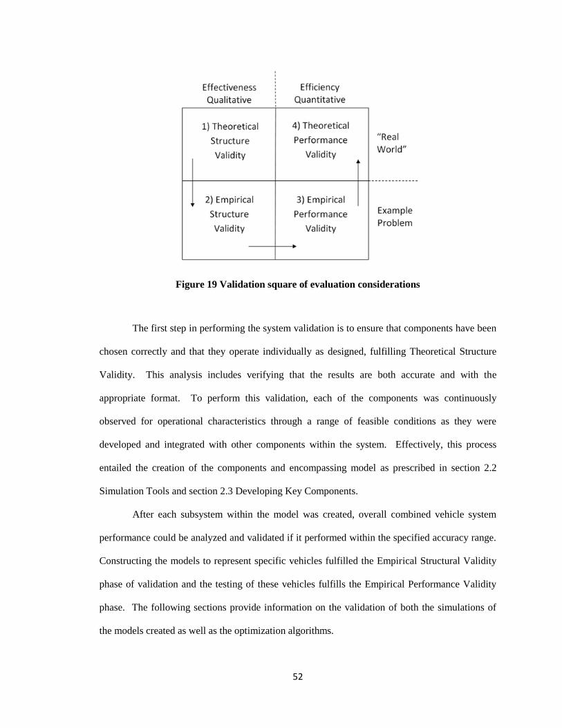
52
Figure 19 Validation square of evaluation considerations
The first step in performing the system validation is to ensure that components have been
chosen correctly and that they operate individually as designed, fulfilling Theoretical Structure
Validity. This analysis includes verifying that the results are both accurate and with the
appropriate format. To perform this validation, each of the components was continuously
observed for operational characteristics through a range of feasible conditions as they were
developed and integrated with other components within the system. Effectively, this process
entailed the creation of the components and encompassing model as prescribed in section 2.2
Simulation Tools and section 2.3 Developing Key Components.
After each subsystem within the model was created, overall combined vehicle system
performance could be analyzed and validated if it performed within the specified accuracy range.
Constructing the models to represent specific vehicles fulfilled the Empirical Structural Validity
phase of validation and the testing of these vehicles fulfills the Empirical Performance Validity
phase. The following sections provide information on the validation of both the simulations of
the models created as well as the optimization algorithms.
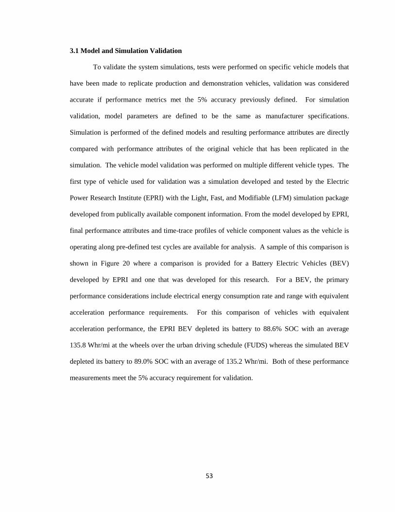
53
3.1 Model and Simulation Validation
To validate the system simulations, tests were performed on specific vehicle models that
have been made to replicate production and demonstration vehicles, validation was considered
accurate if performance metrics met the 5% accuracy previously defined. For simulation
validation, model parameters are defined to be the same as manufacturer specifications.
Simulation is performed of the defined models and resulting performance attributes are directly
compared with performance attributes of the original vehicle that has been replicated in the
simulation. The vehicle model validation was performed on multiple different vehicle types. The
first type of vehicle used for validation was a simulation developed and tested by the Electric
Power Research Institute (EPRI) with the Light, Fast, and Modifiable (LFM) simulation package
developed from publically available component information. From the model developed by EPRI,
final performance attributes and time-trace profiles of vehicle component values as the vehicle is
operating along pre-defined test cycles are available for analysis. A sample of this comparison is
shown in Figure 20 where a comparison is provided for a Battery Electric Vehicles (BEV)
developed by EPRI and one that was developed for this research. For a BEV, the primary
performance considerations include electrical energy consumption rate and range with equivalent
acceleration performance requirements. For this comparison of vehicles with equivalent
acceleration performance, the EPRI BEV depleted its battery to 88.6% SOC with an average
135.8 Whr/mi at the wheels over the urban driving schedule (FUDS) whereas the simulated BEV
depleted its battery to 89.0% SOC with an average of 135.2 Whr/mi. Both of these performance
measurements meet the 5% accuracy requirement for validation.
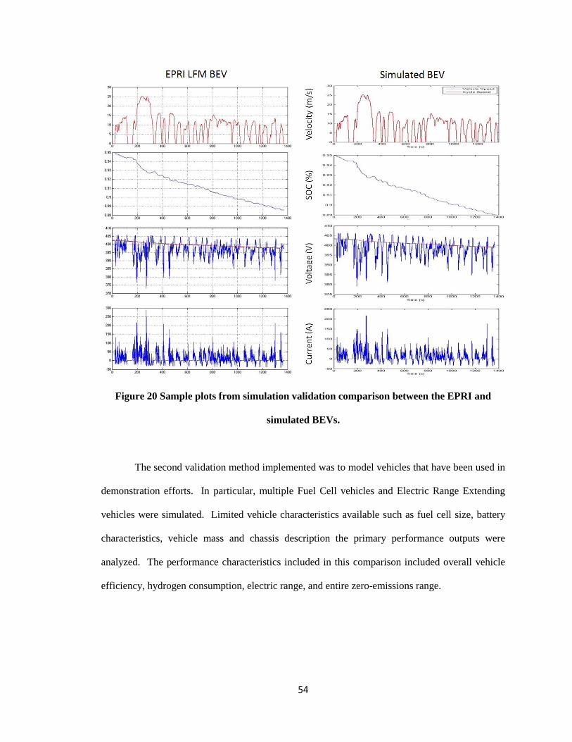
54
Figure 20 Sample plots from simulation validation comparison between the EPRI and
simulated BEVs.
The second validation method implemented was to model vehicles that have been used in
demonstration efforts. In particular, multiple Fuel Cell vehicles and Electric Range Extending
vehicles were simulated. Limited vehicle characteristics available such as fuel cell size, battery
characteristics, vehicle mass and chassis description the primary performance outputs were
analyzed. The performance characteristics included in this comparison included overall vehicle
efficiency, hydrogen consumption, electric range, and entire zero-emissions range.
55
Figure 21 Comparison of vehicle operational parameters used in simulation validation for a
Toyota Prius with data from ANL Downloadable Dynamometer.
The final method used for vehicle comparison was to replicate production vehicles. The
vehicles that were chosen for this comparison were a Toyota Prius and a Chevrolet Volt. Specific
operational characteristics for the Chevrolet Volt were unavailable at the time this study was
completed, but theoretical comparisons can be made with manufacturer reported values for the
vehicle as it undergoes development. Performance characteristics similar to those observed in the
previous Fuel Cell and Electric Range Extending vehicle tests were analyzed. For the simulated
2007 Toyota Prius validation comparison [23, 37, 38], 1 Hz testing data was obtained from the
Argonne National Laboratory’s Downloadable Dynamometer Database [39] which includes the
time samples outputs of a few of the primary operational components. A sample of the
56
comparison made for the Prius is shown in Figure 21. The performance of the simulated Prius’s
components along a time scale are not and were not expected to match the dynamometer data
exactly due to differing control strategies of the epicyclical gear train. Both of the vehicles were
proven to operate over the provided urban driving schedule and achieved accurate fuel economies
of 60.75 mpg for the dynamometer data and 60.95 for the simulated Prius, which meets the 5%
accuracy requirement.
3.2 Validation of Optimization Algorithms
The optimization algorithms that have been selected; Simulated Annealing, Divided
Rectangles, Genetic Algorithm, and Particle Swarm Optimization, must be tested to verify
performance. Each of the algorithms has previously been tested by their developers to verify that
they are capable of identifying local minima in a global search optimization given a sufficient
number of function evaluations. Some of the tests performed included running each optimization
on field standard test functions such as the “Six Hump Camel”, “Rosenbrock”, and “Goldstein-
Price” which each contain multiple local minima, global minima, and dimensions [40].
Of primary importance for validation in this study is the performance of the optimization
algorithms using vehicle simulations. Previous work performed by Gao (et al.) [40] tested the
performance of each of the four algorithms selected in optimizing a six dimensional vehicle
design problem during 400 function evaluations using a parallel type vehicle architecture. The
design variables used in the optimizations performed by Gao included both controller specific and
component specific applications which were Battery State of Charge Maximum, Battery State of
Charge Minimum, ICE Power Limit, EM Power Limit, Final Drive Ratio, and Batter Number of
Cells. The design space upper and lower bounds are shown in Table 2.
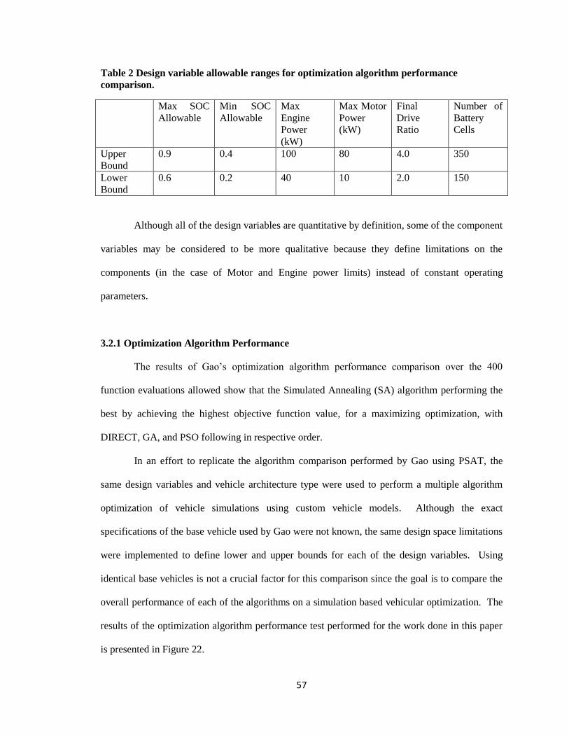
57
Table 2 Design variable allowable ranges for optimization algorithm performance
comparison.
Max SOC
Allowable
Min SOC
Allowable
Max
Engine
Power
(kW)
Max Motor
Power
(kW)
Final
Drive
Ratio
Number of
Battery
Cells
Upper
Bound
0.9 0.4 100 80 4.0 350
Lower
Bound
0.6 0.2 40 10 2.0 150
Although all of the design variables are quantitative by definition, some of the component
variables may be considered to be more qualitative because they define limitations on the
components (in the case of Motor and Engine power limits) instead of constant operating
parameters.
3.2.1 Optimization Algorithm Performance
The results of Gao’s optimization algorithm performance comparison over the 400
function evaluations allowed show that the Simulated Annealing (SA) algorithm performing the
best by achieving the highest objective function value, for a maximizing optimization, with
DIRECT, GA, and PSO following in respective order.
In an effort to replicate the algorithm comparison performed by Gao using PSAT, the
same design variables and vehicle architecture type were used to perform a multiple algorithm
optimization of vehicle simulations using custom vehicle models. Although the exact
specifications of the base vehicle used by Gao were not known, the same design space limitations
were implemented to define lower and upper bounds for each of the design variables. Using
identical base vehicles is not a crucial factor for this comparison since the goal is to compare the
overall performance of each of the algorithms on a simulation based vehicular optimization. The
results of the optimization algorithm performance test performed for the work done in this paper
is presented in Figure 22.
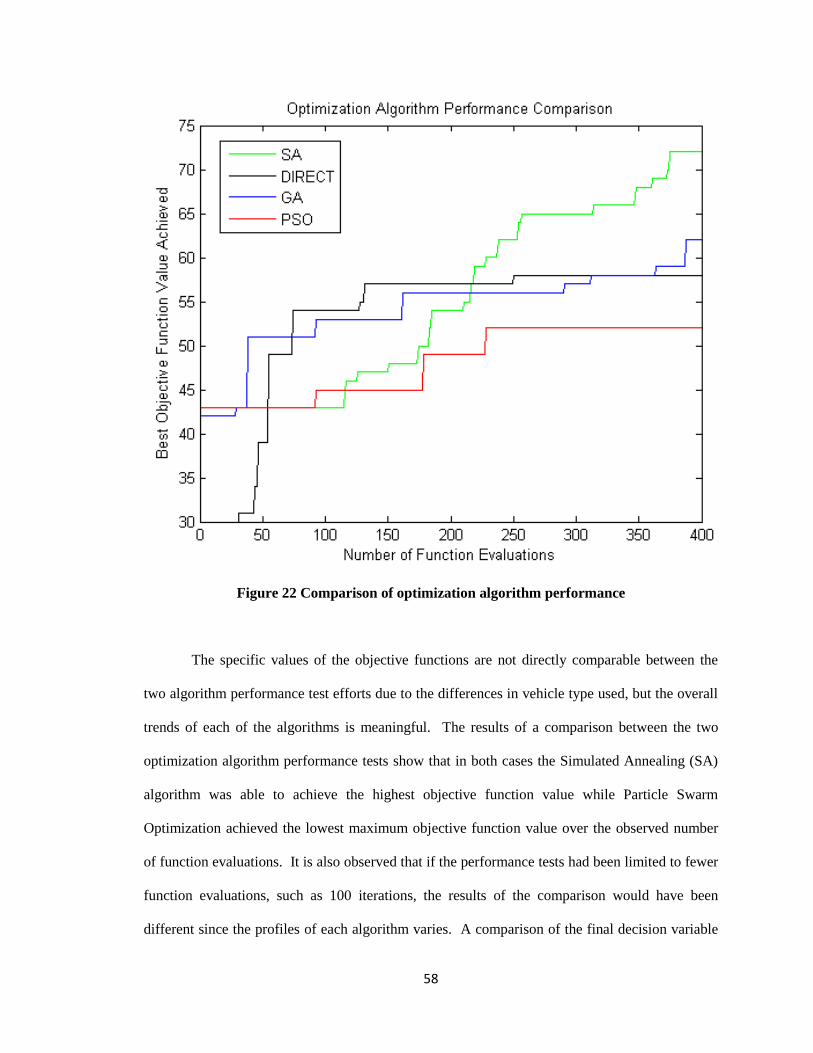
58
Figure 22 Comparison of optimization algorithm performance
The specific values of the objective functions are not directly comparable between the
two algorithm performance test efforts due to the differences in vehicle type used, but the overall
trends of each of the algorithms is meaningful. The results of a comparison between the two
optimization algorithm performance tests show that in both cases the Simulated Annealing (SA)
algorithm was able to achieve the highest objective function value while Particle Swarm
Optimization achieved the lowest maximum objective function value over the observed number
of function evaluations. It is also observed that if the performance tests had been limited to fewer
function evaluations, such as 100 iterations, the results of the comparison would have been
different since the profiles of each algorithm varies. A comparison of the final decision variable
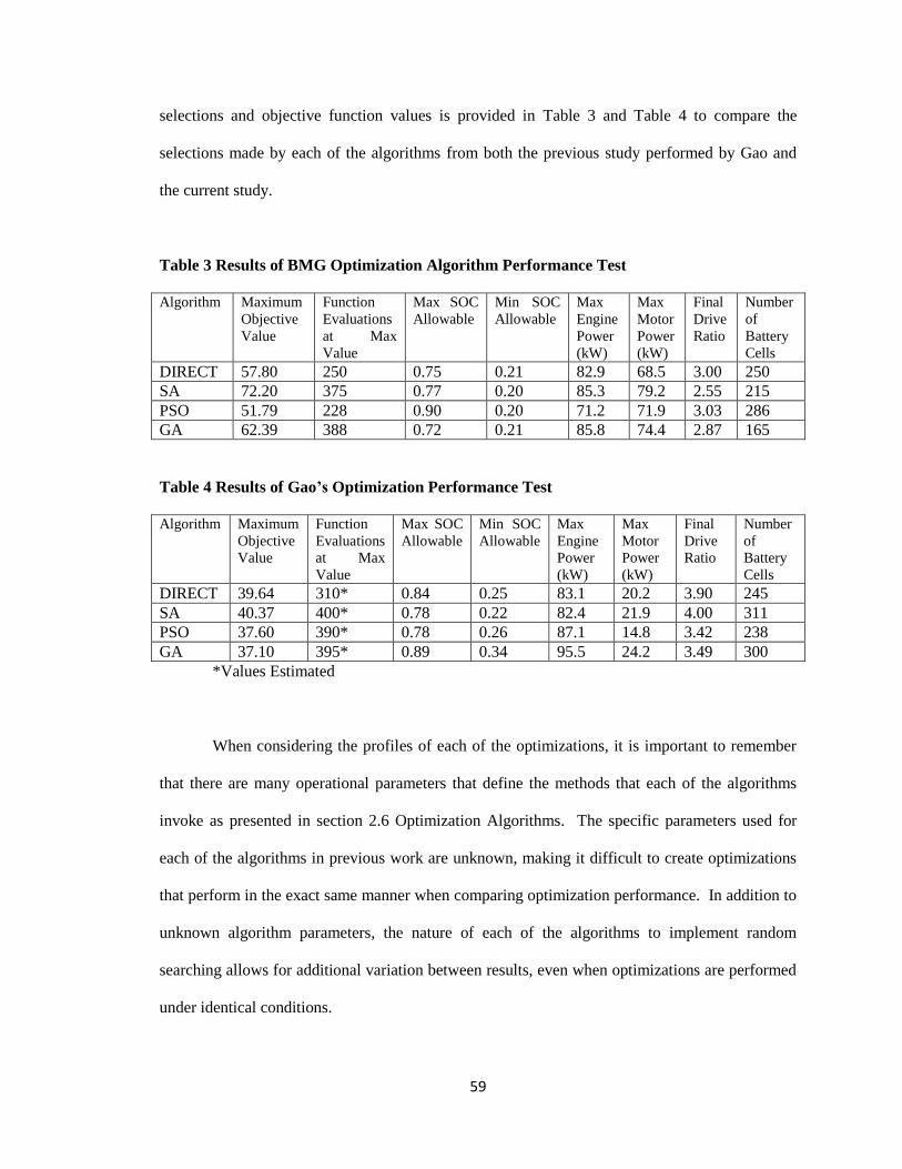
59
selections and objective function values is provided in Table 3 and Table 4 to compare the
selections made by each of the algorithms from both the previous study performed by Gao and
the current study.
Table 3 Results of BMG Optimization Algorithm Performance Test
Algorithm Maximum
Objective
Value
Function
Evaluations
at Max
Value
Max SOC
Allowable
Min SOC
Allowable
Max
Engine
Power
(kW)
Max
Motor
Power
(kW)
Final
Drive
Ratio
Number
of
Battery
Cells
DIRECT 57.80 250 0.75 0.21 82.9 68.5 3.00 250
SA 72.20 375 0.77 0.20 85.3 79.2 2.55 215
PSO 51.79 228 0.90 0.20 71.2 71.9 3.03 286
GA 62.39 388 0.72 0.21 85.8 74.4 2.87 165
Table 4 Results of Gao’s Optimization Performance Test
Algorithm Maximum
Objective
Value
Function
Evaluations
at Max
Value
Max SOC
Allowable
Min SOC
Allowable
Max
Engine
Power
(kW)
Max
Motor
Power
(kW)
Final
Drive
Ratio
Number
of
Battery
Cells
DIRECT 39.64 310* 0.84 0.25 83.1 20.2 3.90 245
SA 40.37 400* 0.78 0.22 82.4 21.9 4.00 311
PSO 37.60 390* 0.78 0.26 87.1 14.8 3.42 238
GA 37.10 395* 0.89 0.34 95.5 24.2 3.49 300
*Values Estimated
When considering the profiles of each of the optimizations, it is important to remember
that there are many operational parameters that define the methods that each of the algorithms
invoke as presented in section 2.6 Optimization Algorithms. The specific parameters used for
each of the algorithms in previous work are unknown, making it difficult to create optimizations
that perform in the exact same manner when comparing optimization performance. In addition to
unknown algorithm parameters, the nature of each of the algorithms to implement random
searching allows for additional variation between results, even when optimizations are performed
under identical conditions.
60
3.2.2 Optimization Algorithm Consistency
When considering the validation and performance characterization of optimization
algorithms it is important to test for consistency. The heuristic-stochastic methods implemented
in the SA, PSO, and GA provides a chance for the algorithms to perform differently on
subsequent optimizations even when identical design space, objectives, and constraints are used.
Although the algorithms were initially classified based on performance in the preceding section,
additional optimizations were performed using each of the algorithms on a different design
simulation to observe repeated performance for consistency. The DIRECT optimization
algorithm is included in the following analysis simply for basis comparison. The deterministic
method implemented by DIRECT ensures that identical optimization search paths will be used on
subsequent optimization runs of the same design space. Therefore, the DIRECT optimization
algorithm can be considered to have 100% consistency because the same solution will always be
found for a given number of function evaluations of identical simulations and design spaces.
Two primary observations are desired through the additional optimizations; the
consistency of the final solutions as well as consistency of the overall optimization profile trace;
and does the algorithm perform with consistent advancement for continued iteration or simply get
lucky occasionally? Together these performance metrics allow for a qualification of each
algorithm’s robustness to the complex design space. Because of the stochastic nature of the
algorithms there is a possibility that the algorithms may begin their search in a highly desired
area, but also the possibility that they may begin in an undesirable design. The examples where
the algorithms begin in the poor design areas are of much more interest for performance
comparisons. If the algorithm can consistently identify more desirable designs when starting in a
poor design area, it is more likely to achieve good designs in future efforts. In contrast, an
optimization that begins its search in a desirable design area, although it started there randomly,
cannot be evaluated effectively for performance. This consideration is made since each of the
stochastic methods has equal probability of starting in the more desirable design locations if they
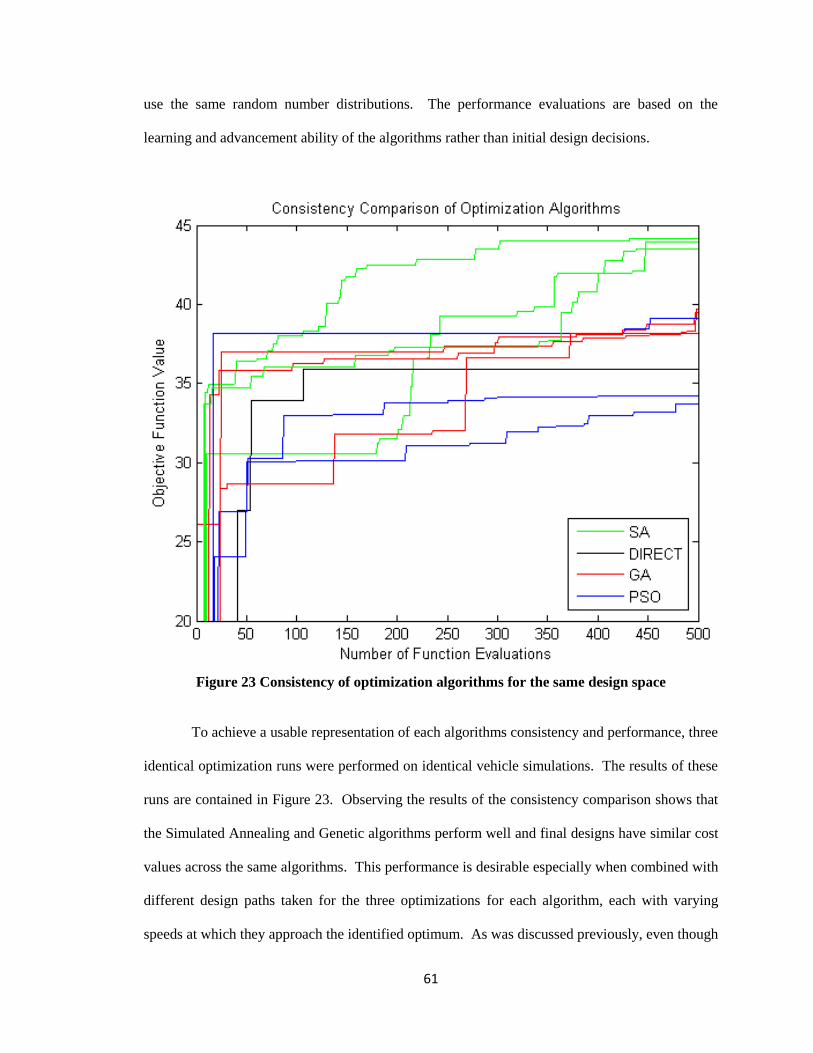
61
use the same random number distributions. The performance evaluations are based on the
learning and advancement ability of the algorithms rather than initial design decisions.
Figure 23 Consistency of optimization algorithms for the same design space
To achieve a usable representation of each algorithms consistency and performance, three
identical optimization runs were performed on identical vehicle simulations. The results of these
runs are contained in Figure 23. Observing the results of the consistency comparison shows that
the Simulated Annealing and Genetic algorithms perform well and final designs have similar cost
values across the same algorithms. This performance is desirable especially when combined with
different design paths taken for the three optimizations for each algorithm, each with varying
speeds at which they approach the identified optimum. As was discussed previously, even though

62
the Particle Swarm Optimization has one instance that achieves a higher objective value than the
other two, it can be seen that this design was located early in the search and may be attributed to
the random search methods. In general the PSO algorithm performs poorly on the sample design
problem.
The validation of the optimization algorithms show that the Simulated Annealing
algorithm performs the best both in terms of objective function value achieved and consistency.
The Genetic Algorithm performs the second best with similar consistency but lower objective
values identified. Divided Rectangles shows perfect consistency but achieves the second lowest
final objective function value over the number of function evaluations observed. The Particle
Swarm Optimization performs the poorest over the design space and function evaluations used in
the validation. Simulated Annealing will be used in the following sections because of its
performance and consistency during the validation.
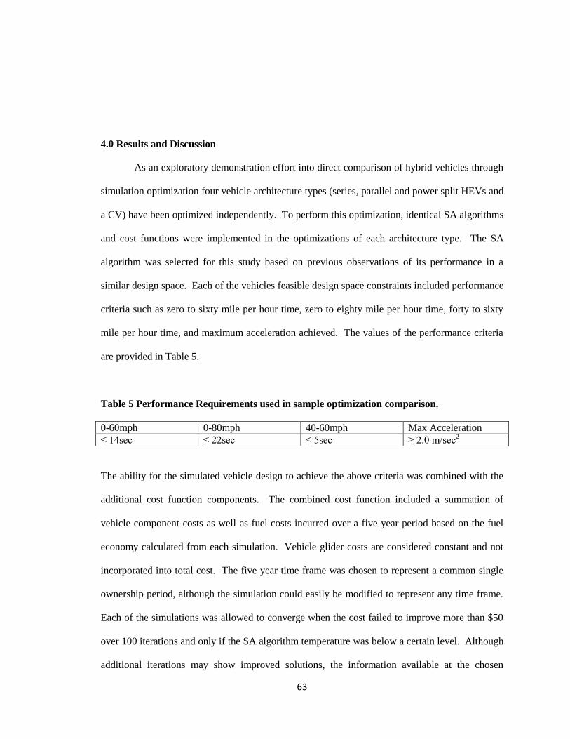
63
4.0 Results and Discussion
As an exploratory demonstration effort into direct comparison of hybrid vehicles through
simulation optimization four vehicle architecture types (series, parallel and power split HEVs and
a CV) have been optimized independently. To perform this optimization, identical SA algorithms
and cost functions were implemented in the optimizations of each architecture type. The SA
algorithm was selected for this study based on previous observations of its performance in a
similar design space. Each of the vehicles feasible design space constraints included performance
criteria such as zero to sixty mile per hour time, zero to eighty mile per hour time, forty to sixty
mile per hour time, and maximum acceleration achieved. The values of the performance criteria
are provided in Table 5.
Table 5 Performance Requirements used in sample optimization comparison.
0-60mph 0-80mph 40-60mph Max Acceleration
≤ 14sec ≤ 22sec ≤ 5sec ≥ 2.0 m/sec2
The ability for the simulated vehicle design to achieve the above criteria was combined with the
additional cost function components. The combined cost function included a summation of
vehicle component costs as well as fuel costs incurred over a five year period based on the fuel
economy calculated from each simulation. Vehicle glider costs are considered constant and not
incorporated into total cost. The five year time frame was chosen to represent a common single
ownership period, although the simulation could easily be modified to represent any time frame.
Each of the simulations was allowed to converge when the cost failed to improve more than $50
over 100 iterations and only if the SA algorithm temperature was below a certain level. Although
additional iterations may show improved solutions, the information available at the chosen
64
convergence is sufficient to make preliminary analysis of the data to show the utility of using the
methods outlined in this work. Definitive optimization efforts for specific vehicle types and
constraints may wish to increase the convergence criteria to allow for more possible iterations.
4.1 Design Space Analysis
One of the advantages of performing optimizations of the selected vehicles is increasing
the amount of information about the designs within the provided design space. By performing
many simulations, with global optimization efforts covering a wide range of designs within the
design space, interpretive mappings of the design space can be made. With these maps it is
possible to identify specific regions of the design space which may be desirable or undesirable
relative to the defined objectives. Additionally, preliminary observations of the design space
mappings allow for quasi-validation of the necessity for utilization of the heuristic-stochastic
optimization algorithm as opposed to other algorithms such as gradient based or statistical
optimizers. Observations of nonlinearities, multiple minima and maxima, as well as an
integration of the objective function as it is defined allow for a classification of the design space.
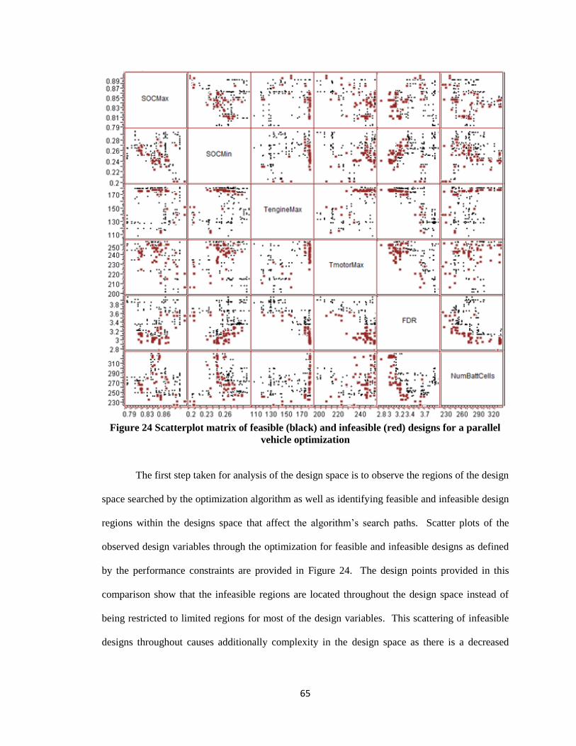
65
Figure 24 Scatterplot matrix of feasible (black) and infeasible (red) designs for a parallel
vehicle optimization
The first step taken for analysis of the design space is to observe the regions of the design
space searched by the optimization algorithm as well as identifying feasible and infeasible design
regions within the designs space that affect the algorithm’s search paths. Scatter plots of the
observed design variables through the optimization for feasible and infeasible designs as defined
by the performance constraints are provided in Figure 24. The design points provided in this
comparison show that the infeasible regions are located throughout the design space instead of
being restricted to limited regions for most of the design variables. This scattering of infeasible
designs throughout causes additionally complexity in the design space as there is a decreased
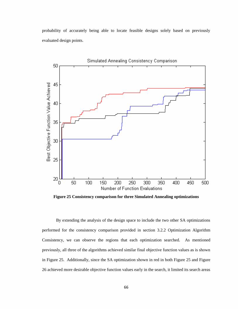
66
probability of accurately being able to locate feasible designs solely based on previously
evaluated design points.
Figure 25 Consistency comparison for three Simulated Annealing optimizations
By extending the analysis of the design space to include the two other SA optimizations
performed for the consistency comparison provided in section 3.2.2 Optimization Algorithm
Consistency, we can observe the regions that each optimization searched. As mentioned
previously, all three of the algorithms achieved similar final objective function values as is shown
in Figure 25. Additionally, since the SA optimization shown in red in both Figure 25 and Figure
26 achieved more desirable objective function values early in the search, it limited its search areas
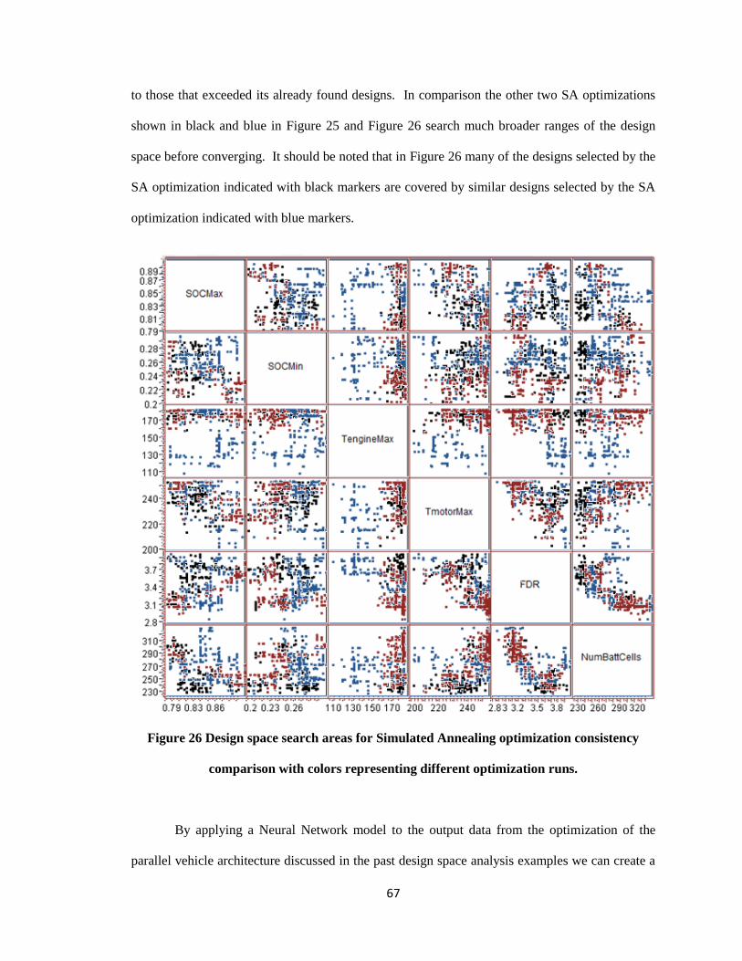
67
to those that exceeded its already found designs. In comparison the other two SA optimizations
shown in black and blue in Figure 25 and Figure 26 search much broader ranges of the design
space before converging. It should be noted that in Figure 26 many of the designs selected by the
SA optimization indicated with black markers are covered by similar designs selected by the SA
optimization indicated with blue markers.
Figure 26 Design space search areas for Simulated Annealing optimization consistency
comparison with colors representing different optimization runs.
By applying a Neural Network model to the output data from the optimization of the
parallel vehicle architecture discussed in the past design space analysis examples we can create a
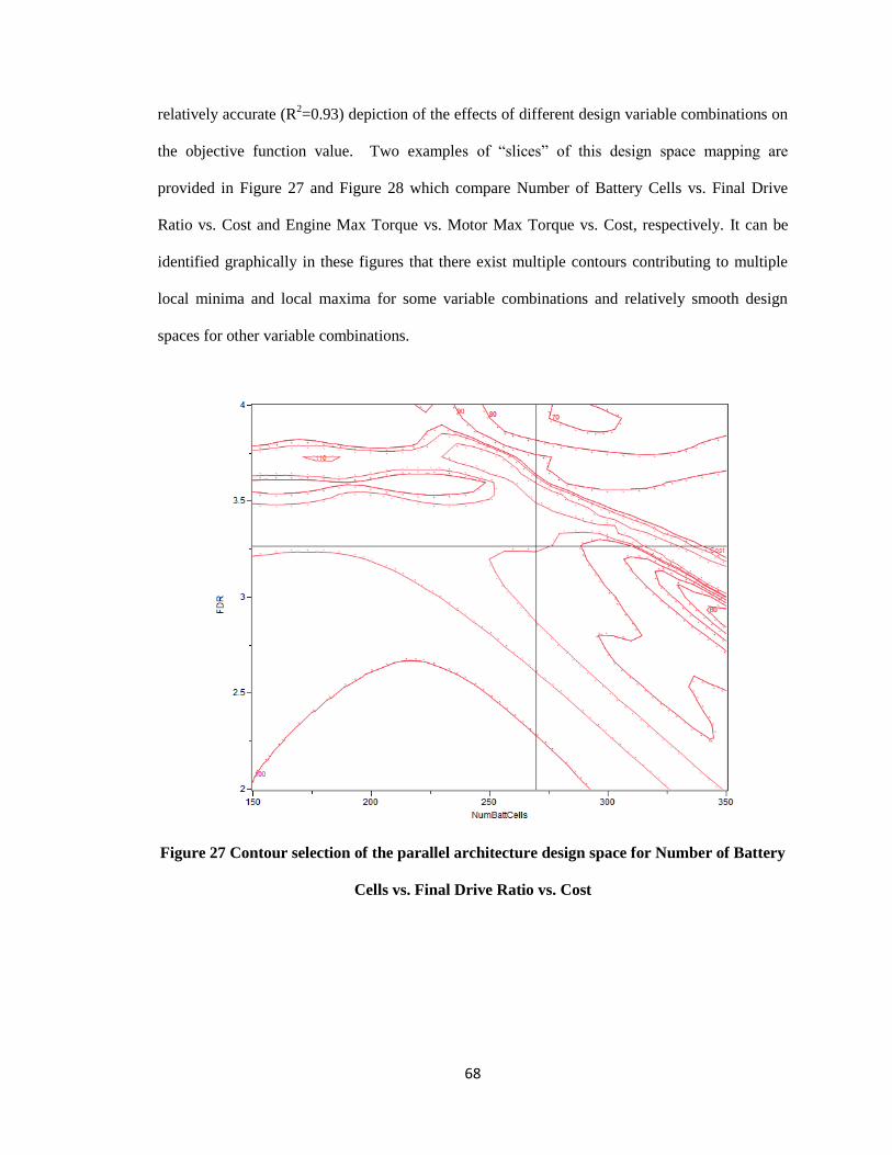
68
relatively accurate (R2=0.93) depiction of the effects of different design variable combinations on
the objective function value. Two examples of “slices” of this design space mapping are
provided in Figure 27 and Figure 28 which compare Number of Battery Cells vs. Final Drive
Ratio vs. Cost and Engine Max Torque vs. Motor Max Torque vs. Cost, respectively. It can be
identified graphically in these figures that there exist multiple contours contributing to multiple
local minima and local maxima for some variable combinations and relatively smooth design
spaces for other variable combinations.
Figure 27 Contour selection of the parallel architecture design space for Number of Battery
Cells vs. Final Drive Ratio vs. Cost
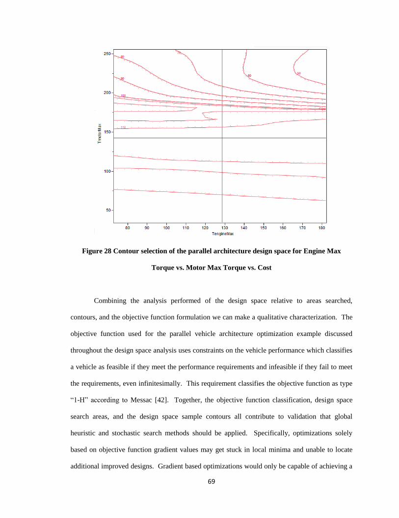
69
Figure 28 Contour selection of the parallel architecture design space for Engine Max
Torque vs. Motor Max Torque vs. Cost
Combining the analysis performed of the design space relative to areas searched,
contours, and the objective function formulation we can make a qualitative characterization. The
objective function used for the parallel vehicle architecture optimization example discussed
throughout the design space analysis uses constraints on the vehicle performance which classifies
a vehicle as feasible if they meet the performance requirements and infeasible if they fail to meet
the requirements, even infinitesimally. This requirement classifies the objective function as type
“1-H” according to Messac [42]. Together, the objective function classification, design space
search areas, and the design space sample contours all contribute to validation that global
heuristic and stochastic search methods should be applied. Specifically, optimizations solely
based on objective function gradient values may get stuck in local minima and unable to locate
additional improved designs. Gradient based optimizations would only be capable of achieving a
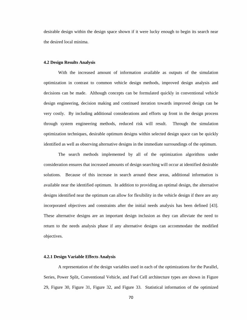
70
desirable design within the design space shown if it were lucky enough to begin its search near
the desired local minima.
4.2 Design Results Analysis
With the increased amount of information available as outputs of the simulation
optimization in contrast to common vehicle design methods, improved design analysis and
decisions can be made. Although concepts can be formulated quickly in conventional vehicle
design engineering, decision making and continued iteration towards improved design can be
very costly. By including additional considerations and efforts up front in the design process
through system engineering methods, reduced risk will result. Through the simulation
optimization techniques, desirable optimum designs within selected design space can be quickly
identified as well as observing alternative designs in the immediate surroundings of the optimum.
The search methods implemented by all of the optimization algorithms under
consideration ensures that increased amounts of design searching will occur at identified desirable
solutions. Because of this increase in search around these areas, additional information is
available near the identified optimum. In addition to providing an optimal design, the alternative
designs identified near the optimum can allow for flexibility in the vehicle design if there are any
incorporated objectives and constraints after the initial needs analysis has been defined [43].
These alternative designs are an important design inclusion as they can alleviate the need to
return to the needs analysis phase if any alternative designs can accommodate the modified
objectives.
4.2.1 Design Variable Effects Analysis
A representation of the design variables used in each of the optimizations for the Parallel,
Series, Power Split, Conventional Vehicle, and Fuel Cell architecture types are shown in Figure
29, Figure 30, Figure 31, Figure 32, and Figure 33. Statistical information of the optimized
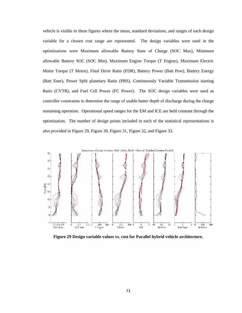
71
vehicle is visible in these figures where the mean, standard deviations, and ranges of each design
variable for a chosen cost range are represented. The design variables were used in the
optimizations were Maximum allowable Battery State of Charge (SOC Max), Minimum
allowable Battery SOC (SOC Min), Maximum Engine Torque (T Engine), Maximum Electric
Motor Torque (T Motor), Final Drive Ratio (FDR), Battery Power (Batt Pow), Battery Energy
(Batt Ener), Power Split planetary Ratio (PRS), Continuously Variable Transmission starting
Ratio (CVTR), and Fuel Cell Power (FC Power). The SOC design variables were used as
controller constraints to determine the range of usable batter depth of discharge during the charge
sustaining operation. Operational speed ranges for the EM and ICE are held constant through the
optimization. The number of design points included in each of the statistical representations is
also provided in Figure 29, Figure 30, Figure 31, Figure 32, and Figure 33.
Figure 29 Design variable values vs. cost for Parallel hybrid vehicle architecture.
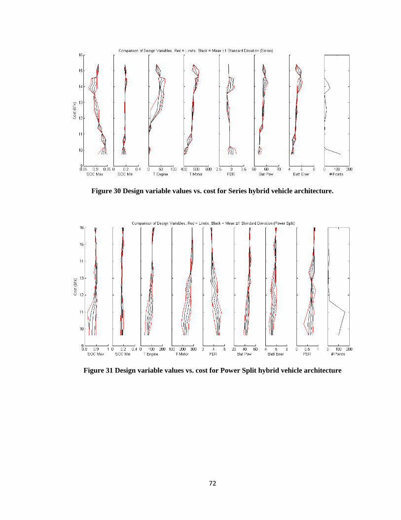
72
Figure 30 Design variable values vs. cost for Series hybrid vehicle architecture.
Figure 31 Design variable values vs. cost for Power Split hybrid vehicle architecture
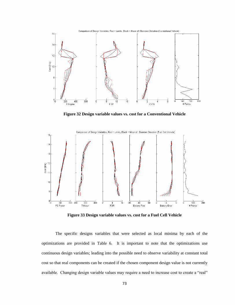
73
Figure 32 Design variable values vs. cost for a Conventional Vehicle
Figure 33 Design variable values vs. cost for a Fuel Cell Vehicle
The specific designs variables that were selected as local minima by each of the
optimizations are provided in Table 6. It is important to note that the optimizations use
continuous design variables; leading into the possible need to observe variability at constant total
cost so that real components can be created if the chosen component design value is not currently
available. Changing design variable values may require a need to increase cost to create a “real”
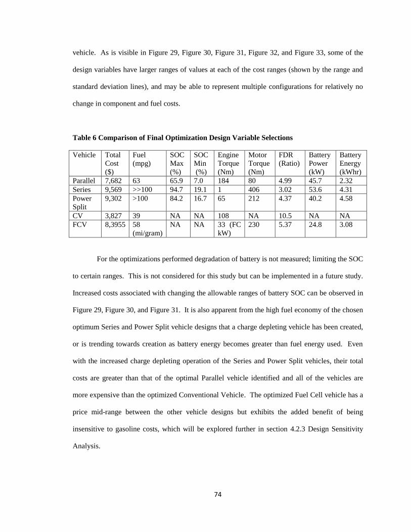
74
vehicle. As is visible in Figure 29, Figure 30, Figure 31, Figure 32, and Figure 33, some of the
design variables have larger ranges of values at each of the cost ranges (shown by the range and
standard deviation lines), and may be able to represent multiple configurations for relatively no
change in component and fuel costs.
Table 6 Comparison of Final Optimization Design Variable Selections
Vehicle Total
Cost
($)
Fuel
(mpg)
SOC
Max
(%)
SOC
Min
(%)
Engine
Torque
(Nm)
Motor
Torque
(Nm)
FDR
(Ratio)
Battery
Power
(kW)
Battery
Energy
(kWhr)
Parallel 7,682 63 65.9 7.0 184 80 4.99 45.7 2.32
Series 9,569 >>100 94.7 19.1 1 406 3.02 53.6 4.31
Power
Split
9,302 >100 84.2 16.7 65 212 4.37 40.2 4.58
CV 3,827 39 NA NA 108 NA 10.5 NA NA
FCV 8,3955 58
(mi/gram)
NA NA 33 (FC
kW)
230 5.37 24.8 3.08
For the optimizations performed degradation of battery is not measured; limiting the SOC
to certain ranges. This is not considered for this study but can be implemented in a future study.
Increased costs associated with changing the allowable ranges of battery SOC can be observed in
Figure 29, Figure 30, and Figure 31. It is also apparent from the high fuel economy of the chosen
optimum Series and Power Split vehicle designs that a charge depleting vehicle has been created,
or is trending towards creation as battery energy becomes greater than fuel energy used. Even
with the increased charge depleting operation of the Series and Power Split vehicles, their total
costs are greater than that of the optimal Parallel vehicle identified and all of the vehicles are
more expensive than the optimized Conventional Vehicle. The optimized Fuel Cell vehicle has a
price mid-range between the other vehicle designs but exhibits the added benefit of being
insensitive to gasoline costs, which will be explored further in section 4.2.3 Design Sensitivity
Analysis.
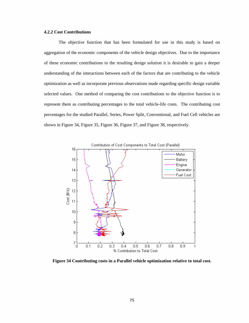
75
4.2.2 Cost Contributions
The objective function that has been formulated for use in this study is based on
aggregation of the economic components of the vehicle design objectives. Due to the importance
of these economic contributions to the resulting design solution it is desirable to gain a deeper
understanding of the interactions between each of the factors that are contributing to the vehicle
optimization as well as incorporate previous observations made regarding specific design variable
selected values. One method of comparing the cost contributions to the objective function is to
represent them as contributing percentages to the total vehicle-life costs. The contributing cost
percentages for the studied Parallel, Series, Power Split, Conventional, and Fuel Cell vehicles are
shown in Figure 34, Figure 35, Figure 36, Figure 37, and Figure 38, respectively.
Figure 34 Contributing costs in a Parallel vehicle optimization relative to total cost.
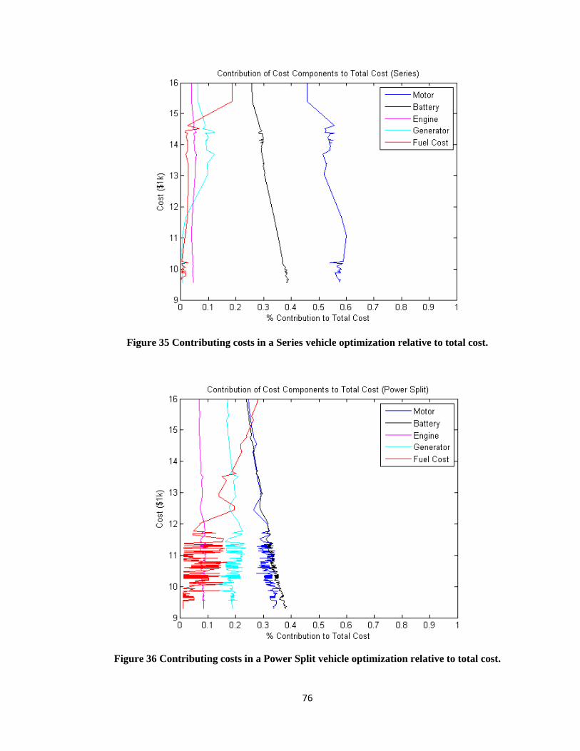
76
Figure 35 Contributing costs in a Series vehicle optimization relative to total cost.
Figure 36 Contributing costs in a Power Split vehicle optimization relative to total cost.
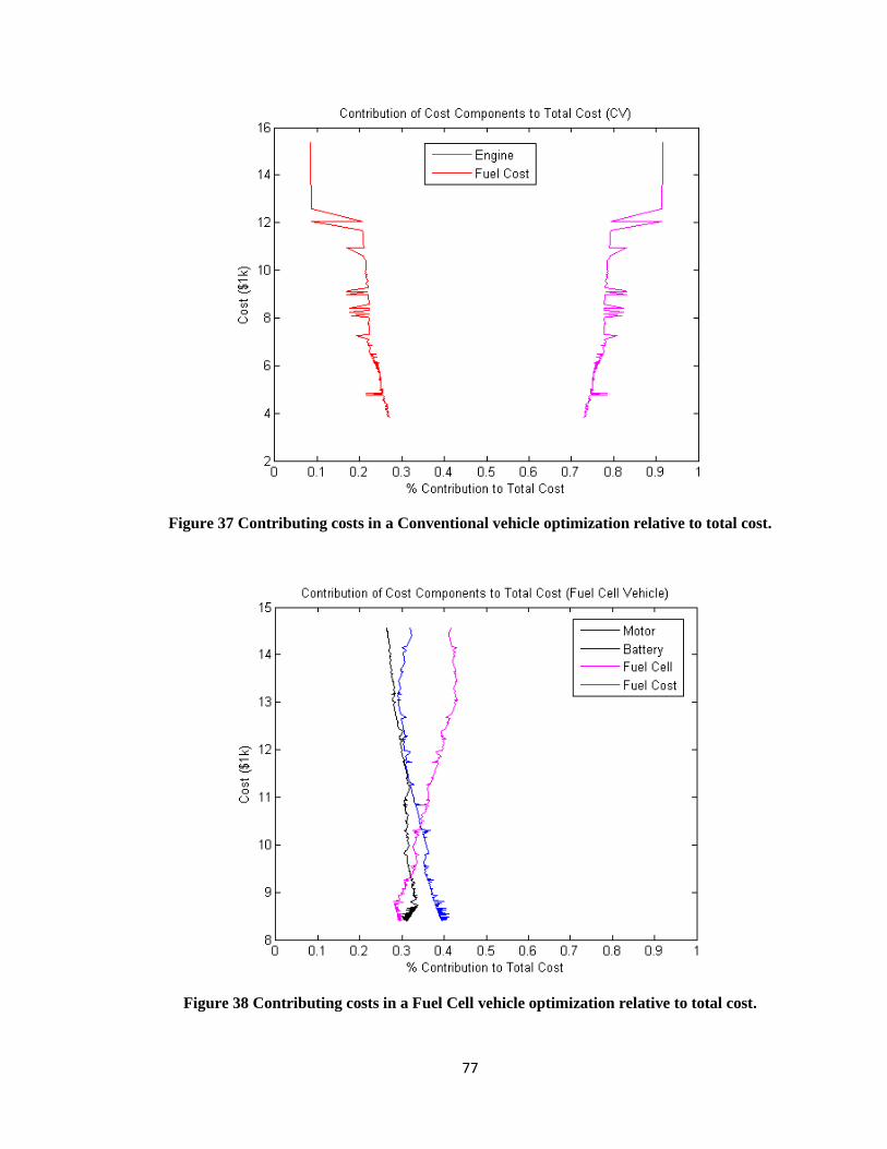
77
Figure 37 Contributing costs in a Conventional vehicle optimization relative to total cost.
Figure 38 Contributing costs in a Fuel Cell vehicle optimization relative to total cost.
78
It can be observed in Figure 34, Figure 35, Figure 36, Figure 37, and Figure 38 that the
Parallel and Fuel Cell vehicle types have cost contribution components that are relatively similar
to one another. This may be contributed to power balancing between drive components available
in the parallel vehicle architecture. Power balancing between components is also a possibility in
the Power Split vehicle architecture as the Motor, ICE, and Generator can all provide tractive
efforts, but in the optimal design the Power Split vehicle appears to be directed towards a design
that is more similar to the Series architecture than the Parallel architecture. In contrast to the
power balancing, the series vehicle architecture optimization shows how the single contributing
tractive effort from the electric motor causes it to be large in order to meet the performance
criteria, but allows for a smaller engine and less fuel consumption. As noted previously, charge
depleting vehicle designs are beginning to emerge through the optimization. Required vehicle
range was not included in the initial design objectives and vehicles were only evaluated on their
ability to perform over drive cycles which were each shorter than 18km (~11mi). This surfacing
of vehicle operation can provide a basis for including additional PHEV-type constraints such as
charge sustaining operation or increased required range to provide for an improved overall
design. The differences in contribution percentages from component costs and fuel costs lead to a
better understanding of the effects of varying associated fuel costs, ownership time period, and
other economic assumptions that were included in the aggregate cost function formulation.
4.2.3 Design Sensitivity Analysis
When discussing the results of any design effort, particularly in optimization, it is useful
to understand the sensitivity of the final design. As an example exploration of the sensitivity of
the vehicles the results of a sensitivity analysis are presented for design selections of the optimal
design variables as well as assumptions that are made. Assumptions made for gasoline fueling
costs as well as ownership time period are provided and analyzed for sensitivity to variation.
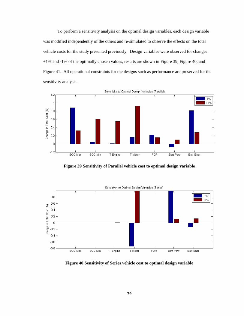
79
To perform a sensitivity analysis on the optimal design variables, each design variable
was modified independently of the others and re-simulated to observe the effects on the total
vehicle costs for the study presented previously. Design variables were observed for changes
+1% and -1% of the optimally chosen values, results are shown in Figure 39, Figure 40, and
Figure 41. All operational constraints for the designs such as performance are preserved for the
sensitivity analysis.
Figure 39 Sensitivity of Parallel vehicle cost to optimal design variable
Figure 40 Sensitivity of Series vehicle cost to optimal design variable
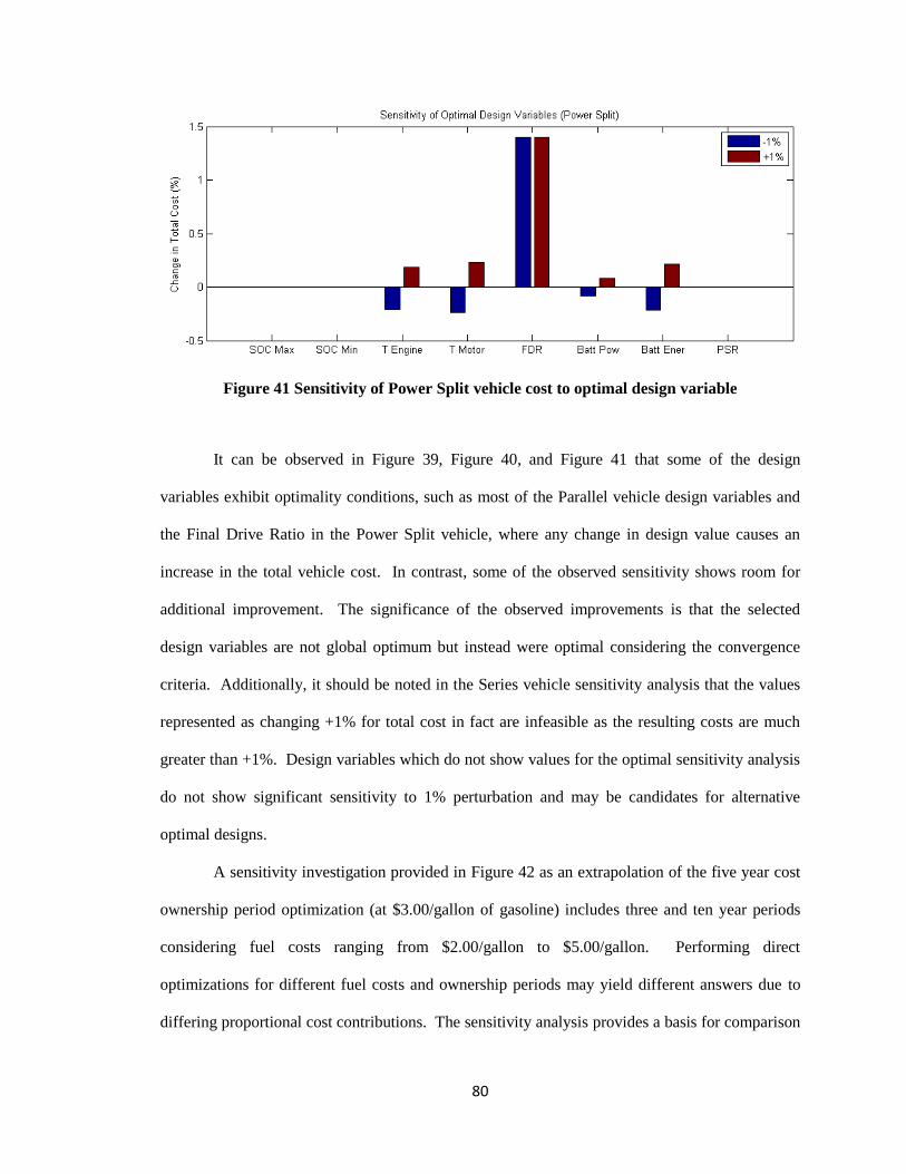
80
Figure 41 Sensitivity of Power Split vehicle cost to optimal design variable
It can be observed in Figure 39, Figure 40, and Figure 41 that some of the design
variables exhibit optimality conditions, such as most of the Parallel vehicle design variables and
the Final Drive Ratio in the Power Split vehicle, where any change in design value causes an
increase in the total vehicle cost. In contrast, some of the observed sensitivity shows room for
additional improvement. The significance of the observed improvements is that the selected
design variables are not global optimum but instead were optimal considering the convergence
criteria. Additionally, it should be noted in the Series vehicle sensitivity analysis that the values
represented as changing +1% for total cost in fact are infeasible as the resulting costs are much
greater than +1%. Design variables which do not show values for the optimal sensitivity analysis
do not show significant sensitivity to 1% perturbation and may be candidates for alternative
optimal designs.
A sensitivity investigation provided in Figure 42 as an extrapolation of the five year cost
ownership period optimization (at $3.00/gallon of gasoline) includes three and ten year periods
considering fuel costs ranging from $2.00/gallon to $5.00/gallon. Performing direct
optimizations for different fuel costs and ownership periods may yield different answers due to
differing proportional cost contributions. The sensitivity analysis provides a basis for comparison
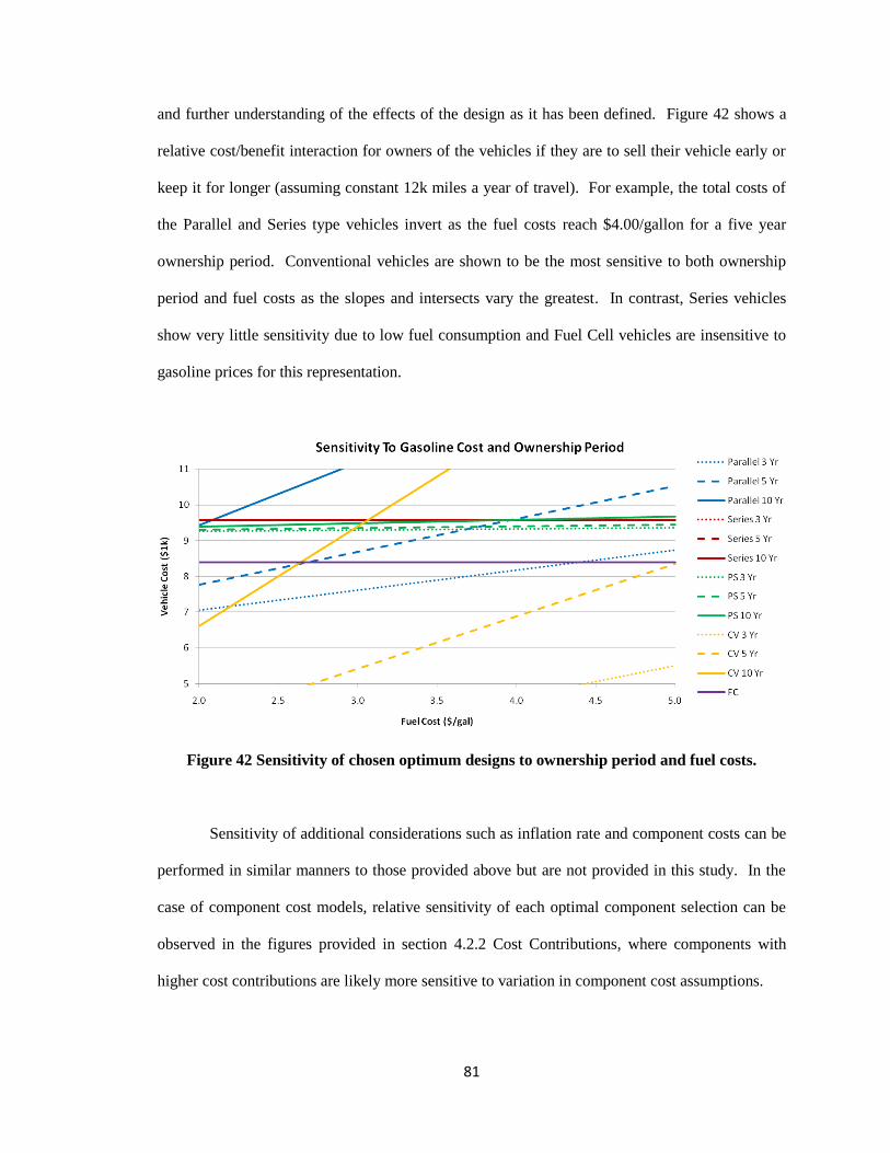
81
and further understanding of the effects of the design as it has been defined. Figure 42 shows a
relative cost/benefit interaction for owners of the vehicles if they are to sell their vehicle early or
keep it for longer (assuming constant 12k miles a year of travel). For example, the total costs of
the Parallel and Series type vehicles invert as the fuel costs reach $4.00/gallon for a five year
ownership period. Conventional vehicles are shown to be the most sensitive to both ownership
period and fuel costs as the slopes and intersects vary the greatest. In contrast, Series vehicles
show very little sensitivity due to low fuel consumption and Fuel Cell vehicles are insensitive to
gasoline prices for this representation.
Figure 42 Sensitivity of chosen optimum designs to ownership period and fuel costs.
Sensitivity of additional considerations such as inflation rate and component costs can be
performed in similar manners to those provided above but are not provided in this study. In the
case of component cost models, relative sensitivity of each optimal component selection can be
observed in the figures provided in section 4.2.2 Cost Contributions, where components with
higher cost contributions are likely more sensitive to variation in component cost assumptions.
82
All of the analysis performed on the sample vehicles, through simulation optimization,
shows the utility of utilizing the optimization tools with well formulated cost functions. Future
efforts to improve the control strategies and further refine the design variables, constraints, and
objectives selection can result in increased understanding of any complex hybrid vehicle system
and design space. This aids in decision making. The specific vehicle design results found
through the vehicle optimizations are not intended to represent finality for all vehicles of that
architecture type, but simply to allow for a comparison in designs for the constraints formulated
in this study.
4.3 Areas of Interest for Continued Efforts
The example optimizations explored through this study bring to light many additional
areas where analysis can be performed with increased implementation of the methods described.
As noted throughout the study method description, validation, and results analysis, the examples
have shown relying limited formulations of the objective function which focus primarily on an
economic quantification of the cost of the vehicle over a single ownership period. As regulations,
standards, and general design understanding increase it is likely that inflating desire to
incorporate system-level design objectives will arise. Determining exactly what these objective
functions will be and which system-, vehicle-, and subsystem-level objectives are included will
be left up to future studies.
As identified through the exploration of the results, there is a need to incorporate
additional design constraints which will aid in identifying vehicle designs that are more likely to
have real-world potential. In continued design studies it is strongly encouraged that as many
design objectives and constraints that can be foreseeable can and should be included to reduce the
risk and costs of re-performing design explorations.
The components that were selected at the subsystem-level of design for use in the vehicle
simulation optimizations was limited in this study to those which are becoming increasingly
83
relevant and understood in today’s hybrid vehicle designs. In future work, it would be desirable
to include additional subsystems such as energy storage flywheels and super capacitors, or power
production systems such as turbines and photovoltaics.
Advancing beyond the subsystem-level flexibility of the proposed system design to the
vehicle-level it is possible to create vehicle simulations and optimizations which are capable of
modifying architectures. In this way, it would be up to the optimizations process to determine
which components are included in the vehicle design as well as how many and their
configurations. This ability would extend beyond the common classification limitations of the
Series, Parallel, and Power Split architectures. An increased level of controller design and
understanding to manage all of the systems together would also be needed for incorporation.
Adding ability for an integrated optimization of the controller within each design configuration
generated by the vehicle optimizer may alleviate some of the efforts to obtain a robust cross-
architectural controller.
This research is not new in all the concepts that it employs but rather in the possibilities
for advancement for a more thorough understanding of vehicle design. Additionally, the areas of
interest for continued effort are much more readily implemented using the methods and tools that
have been explored in depth throughout this paper.
84
5.0 Conclusions
Vehicle design is a resource intensive process; incorporating hybridization introduces
additional design complexities. By applying systems engineering methods such as objective
identification and optimization up-front in the design process it is likely that a desirable solution
will be achieved with minimal costs in both time and effort. Through the use of defensible
vehicle system simulation, aggregate objective cost functions as system engineering tools can be
incorporated to build a better understanding of the design space. Although implementing
simulation optimization into vehicular design is not a new concept, applications and utility have
been expanded to include additional areas which increase understanding and ability to implement
complex designs. A few of the possible assessments that can be taken from a simulation
optimization comparison have been provided for sample vehicle architectures, control styles,
objectives, and constraints.
A set of vehicle design tools including models, simulations, and optimizations have been
presented and explored: providing benefits to future design efforts. In conclusion:
System-level design objectives can be incorporated into advanced vehicle design
through aggregate objective functions.
Systems engineering approaches to vehicle modeling and simulation contribute
to defensible results and analysis.
Global optimization algorithms are necessary to accurately explore the complex
design space of hybrid vehicles.

85
Between the four optimization algorithms tested, Simulated Annealing and
Genetic Algorithm optimization show more promising performance but function
differently within different design efforts.
Vehicle simulation optimization is capable of identifying superior designs with
reduced cost to the design process.
Simulation optimization provides information on design space complexity,
optimal designs, and optimal design sensitivity.
Simulation optimization is a prolific tool for directly comparing different vehicle
designs.
With proper models, simulations, optimization algorithms, and cost functions almost any
vehicle system and design goals can be represented. Future work can be developed to assist
designers by analyzing the complex design interactions. This provides not only a reduction of the
resources necessary to design a car, but also improves the implementation of design objectives in
the design construction process.
Increased understanding of hybrid vehicle design through modeling, simulation, and
optimization allows designers to achieve more desirable solutions. Through the integration of
aggregate cost functions, system-level design objectives can be fulfilled such as costs over the
lifetime of the vehicle. Implementation of the methods presented in this research can allow for
improved designs and reduced risk for the designers.
86
References
1. Geller, B., Quinn, C.W., and Bradley, T.H., "Analysis of Design Tradeoffs for Plug-in
Hybrid Vehicles," in Battery, Hybrid and Fuel Cell Vehicles. Performance, Market and
Environmental Issues, Pistoia, G., Ed., Elsevier, 2010.
2. Wishart, J. D., “Modelling, Simulation, Testing, and Optimization of Advanced Hybrid
Vehicle Powertrains,” Dissertation, University of Victoria, Canada, 2008.
3. Blanchard, B. S., “Systems Engineering and Analysis: Fourth Edition,” Prentice Hall
International Series in Industrial and Systems Engineering, 2006.
4. Kossiakoff, A., and Sweet, W. N., “System Engineering Principles and Practices,” John
Wiley and Sons, 2003.
5. Zhang, Y., Lin, H., Zhang, B., and Mi, C., “Performance Modeling and Optimization of a
Novel Multi-mode Hybrid Powertrain,” ASME Journal of Mechanical Design, April 6,
2005.
6. Yang, C., Li, J., Sun, W., Zhang, B., Gao, Y., and Yin, X., “Study on Global
Optimization of Plug-In Hybrid Electric Vehicle Energy Management Strategies,”
National High Technology Research and Development Program of China, 2006.
7. Gao, W., Mi, C. and Emadi, A., “Modeling and Simulation of Electric and Hybrid
Vehicles,” Proceedings of the IEEE, Vol. 95, No. 4, April, 2007.
8. Zhou, Y. L., “Modeling and Simulation of Hybrid Electric Vehicles,” Thesis, University
of Victoria, Canada, 2005.
9. Tummescheit, H., “Design and Implementation of Object Oriented Model Libraries using
Modelica,” Department of Automatic Control, Lund Institute of Technology, Lund,
Sweden, 2002.
10. Fritzson, P., Aronsson, P., Lundvall, H., Nyström, K., Pop, A., Saldamli, L., and Broman,
D., “The OpenModelica Modeling, Simulation, and Development Environment,” PELAB
– Programming Environment Lab, Dept. Computer Science, Linköping University, S-581
83, Linköping, Sweden, 2005.
11. Wallén, J., “Modelling of Components for Conventional Car and Hybrid Electric Vehicle
in Modelica,” Thesis, Linköping University, May 10, 2004.
12. Fröberg, A., “Extending the Inverse Vehicle Propulsion Simulation Concept –To Improve
Simulation Performance,” Linköping Studies in Science and Technolgy, Thesis No.
1181, Department of Electrical Engineering, Linköping University, S-581 83, Linköping,
Sweden, 2005.
13. Bradley, T.H. and Frank, A.A., “Design, demonstration and sustainability impact
assessments for plug-in hybrid electric vehicles,” Renewable & Sustainable Energy
Reviews, doi:10.1016/j.rser.2007.05.003, 2007.
87
14. Ehsani, M., Gao, Y., and Miller, J. M., “Hybrid Electric Vehicles: Architecture and
Motor Drives,” Proceedings of the IEEE, Vol. 95, No. 4, April, 2007.
15. Duoba, M., Carlson, R., and Bocci, D., “Calculating Results and Performance
Parameters for PHEVs,” SAE 2009-01-1328, 2009.
16. An, F., Frank, A., and Ross, H., “Meeting both ZEV and PNGV Goals with a Hybrid
Electric Vehicle: An Exploration,” SAE, 1996.
17. “Comparing the Benefits and Impacts of Hybrid Electric Vehicle Options for Compact
Sedan and Sport Utility Vehicles,” Electric Power Research Institute, Palo Alto, CA,
2002.
18. Kalhammer, F.R., Kopf, B.M., Swan, D.H., Roan, V.P., Walsh and M.P., “Status and
Prospects for Zero Emissions Vehicle Technology, Report of the ARB Independent Expert
Panel 2007,” Prepared for State of California Air Resources Board, Sacramento,
California, USA, April, 2007.
19. Pukrushpan, J. T., “Modeling and Control of Fuel Cell Systems and Fuel Processors,”
Dissertation, University of Michigan, Anne Arbor, MI, 2003.
20. “Final Technical Support Document: Fuel Economy Labeling of Motor Vehicle Revisions
to Improve Calculation of Fuel Economy Estimates,” US Environmental Protection
Agency, EPA420-R-06-017, December, 2006.
21. “Recommended Practice For Measuring the Exhaust Emissions and Fuel Economy of
Hybrid Electric Vehicles, Including Plug-In Vehicles,” Society of Automotive Engineers,
J11711, June, 2010.
22. “Utility Factor Definitions for Plug-in Hybrid Electric Vehicles Using 2001 U.S. DOT
National Household Travel Survey Data,” Society of Automotive Engineers, J2841,
2009.
23. “Plug-in Fuel Cell Vehicle Technology and Value Analysis Phase 1: Preliminary
Findings and Plan for Detailed Study,” Electric Power Research Institute, Palo Alto, CA:
2010. 1021482.
24. Carson, Y., and Maria, A., “Simulation Optimization: Methods and Applications,”
Proceedings of the 1997 Winter Simulation Conference, 1997.
25. Gao, W. and Porandla, S.K., “Design Optimization of a Parallel Hybrid Electric
Powertrain,” IEEE, Center for Advanced Vehicular Systems, Mississippi State
University, MS, USA, 2005.
26. Finkel, D. E., “DIRECT Optimization Algorithm User Guide,” Center for Research in
Scientific Computation, North Carolina State University, Raleigh, NC, March 2, 1003.
27. Fang, L., and Qin, S., “Concurrent Optimization for Parameters of Powertrain and
Control System of Hybrid Electric Vehicle Based on Multi-Objective Genetic
Algorithms,” SICE-ICASE International Joint Conference, Bexco, Busan, Korea, October
18-21, 2006.
88
28. Wang, Z., Huang, B., Li, W., and Xu, Y., “Particle Swarm Optimization for Operational
Parameters of Series Hybrid Electric Vehicle,” Proceedings of the 2006 IEEE
International Conference on Robotics and Biomimetics, Kumming, China, Devember 17-
20, 2006.
29. Golbuff, S., “Optimization of a Plug-in Hybrid Electric Vehicle,” Thesis, Georgia
Institute of Technology, August 2006.
30. Wong, Y. S., Chau, K. T., and Chan, C. C., “Battery Sizing for Plug-in Hybrid Electric
Vehicles,” Journal of Asian Electric Vehicles, Vol. 4, No. 2, December, 2006.
31. “Comparing the Benefits and Impacts of Hybrid Electric Vehicle Options,” Electric
Power Research Institute, Palo Alto, CA: 2001. 1000349.
32. Same, A., Stipe, A., Gossman, D., and Park, J. W., “A study on optimization of hybrid
drive train using Advanced Vehicle Simulator (ADVISOR),” Journal of Power Sources
195 6954-6963, April, 2010.
33. Stermole, F. J., and Stermole, J. M., “Economic Evaluation and Investment Decision
Methods,” Investment Evaluations Corp, Golden, Colorado, 1996.
34. Karbowski, D., Rousseau, A., Pagerit, S., and Sharer, P., “Plug-In Vehicle Control
Strategy: From Global Optimization to Real-Time Application,” Argonne National
Laboratory, 2007.
35. Seepersad, C. C., Pedersen, K., Emblemsvåg, J., Bailey, R., Allen, J. K., and Mistree, F.,
“The Validation Square: How Does One Verify And Validate A Design Method?,”
Georgia Institute of Technology, 30332-0405, 2005.
36. Liu, J. and Peng, H., “Modeling and Control of a Power-Split Hybrid Vehicle,” IEEE
Transactions on Control Systems Technology, Vol. 16., No. 6, November 2008.
37. Liu, J., Peng, H., and Filipi, Z., “Modeling and Analysis of the Toyota Hybrid System,”
Proceedings of the 2005 IEEE/ASME International Conference on Advanced Intelligent
Mechatronics, Monterey, California, USA, 24-28 July, 2005.
38. Davies, G., “Graham’s Toyota Prius,”
http://prius.ecrostech.com/original/PriusFrames.htm , 26 June, 2002.
39. Argonne National Laboratory Downloadable Dynamometer Database,
https://webapps.anl.gov/vehicle_data, USDOE ANL Transportation Technology R&D
Center, 2010.
40. Björkman, M., and Holmström, K., “Global Optimization Using the DIRECT Algorithm
in Matlab,” Advanced Modeling and Optimization Volume 1, Number 2, 1999.
41. Gao, W. and Mi, C., “Hybrid vehicle design using global optimisation algorithms,” Int. J.
Electric and Hybrid Vehicles, Vol. 1, No. 1, pp.57-70, 2007.

89
42. Messac, A., “From Dubious Construction of Objective Functions to the Application of
Physical Programming,” AIAA Journal, Vol. 38, No. 1, January 2000, pp.155-163.
43. Fellini, R., Michelena, N., Papalambros, P., Sasena, M., “Optimal Design of Automotive
Hybrid Powertrain Systems,” Department of Mechanical Engineering & Applied
Mechanics, The University of Michigan, Ann Arbor, Michigan, 200.