J. theor. Biol. (1992) 155, 201-214

Optimal Selection of Metabolic Fluxes for in vivo Measurement. I. Development of Mathematical Methods

JOANNE M. SAVINELL* AND BERNHARD O. PALSSON t

Cellular Biotechnology Laboratory, Department of Chemical Engineering, The University of Michigan, Ann Arbor, MI 48109-2136, U.S.A.

(Receioed on 16 May 1991, Accepted on 10 October 1991)

The measurement of uptake and secretion rates is often not sufficient to allow the calculation of all internal metabolic fluxes. Measurements of internal fluxes are needed and these additional measurements are used in conjunction with mass-balance equations to calculate the complete metabolic flux map. A method is presented that identifies the fluxes that should be selected for experimental measurement, and the fluxes that can be computed using the mass-balance equations. The criterion for selecting internal metabolic fluxes for measurement is that the values of the computed fluxes should have low sensitivity to experimental error in the measured fluxes. A condition number indicating the upper bound on this sensitivity, is calculated based on stoichiometry alone. The actual sensitivity is dependent on both the flux measure- ments and the error in flux measurements, as well as the stoichiometry. If approxi- mate physiologic ranges of fluxes are known a realistic sensitivity can be computed. The exact sensitivity cannot be calculated since the experimental error is usually unknown. The most probable value of the actual sensitivity for a given selection of measured fluxes is estimated by selecting a large number of representative error vectors and calculating the actual sensitivity for each of these. A frequency distribu- tion of actual sensitivities is thus obtained giving a representative range of actual sensitivities for a particular experimental situation.

Introduction

The study of steady-state fluxes within the cell's metabolic network and the changes in these fluxes in response to enviromental stimuli provides information about the regulation of intermediary metabolism and is important for a number of clinical and biotechnological applications. Metabolic networks can be divided into two general classifications. The first type of network has a large ratio of end products to branch points, so that measurements of product secretion and nutrient uptake rates coupled with mass balances on the intermediates allow the fluxes throughout the network to be estimated. Networks which include only major metabolic and product formation pathways are examples of this type of network. This type of network is commonly used when analyzing bacterial metabolism and product synthesis.

* Present address: Department of Chemical Engineering, Cleveland State University, Cleveland, OH 44115, U.S.A. I" Author to whom correspondence should be addressed.

20t 0022-5193/92/060201 + 14 $03.00/0 © 1992 Academic Press Limited

202 J . M . S A V I N E L L A N D B. O. P A L S S O N

The second type of metabolic network has a large number of branch points and relatively few secreted products. The steady-state fluxes through these networks can- not usually be obtained solely from measurements of the fluxes of components enter- ing and leaving the cell. Additional measurements of fluxes within the cell must normally be made, typically by the use of ~4C labeling or in oivo NMR techniques. Networks describing mammalian cell metabolism and detailed networks of bacterial metabolism are examples of this type of network.

Examples of the first type of metabolic network are found in butanediol and mixed-acid bacteria. The fluxes through these networks have been computed using measurements of the production rates of the fermentation products (Blackwood et al., 1956) and mass-balance equations (Papoutsakis & Meyer, 1985). The uptake and production rates involved with lysine fermentation of Breoibacterium have also been measured (Erickson et al., 1978), and the fluxes within the network calculated (Vailino & Stephanopoulos, 1989). The set of mass balances and data result in an overdetermined system of equations, in which linear regression is used to estimate the unknown fluxes.

Several algorithms have been formulated for studying this type of network. The number of flux measurements that are needed to verify the stoichiometry of the biochemical network was derived (Tsai & Lee, 1988; Niranjan & San, 1989). The consistency of a set of flux measurements can also be checked by means of the mass- balance equations (Papoutsakis & Meyer, 1985). A complete procedure for analyzing this type of network is discussed in (Vallino & Stephanopoulos, 1989). This procedure provides a means for identifying errors in measurements and verifying the appropri- ateness of the steady-state approximation. The condition number of the system is used to determine whether the system is well-posed, and thus whether the fluxes within the network can be calculated based on measurements of uptake and produc- tion rates. A high condition number indicates that the network, as formulated, is ill- posed. The sensitivity of each calculated flux to each measurement can be estimated in order to identify the reactions that should be measured with the greatest accuracy.

In order to estimate the fluxes in the second type of network, i.e. those with a large number of branch points, some of the reaction fluxes within the network must be measured. The common technique is to expose cells to nutrients labeled with 14C, measure the concentrations of intermediates and products with the ~4C label, and then calculate the steady-state fluxes using the mass-balance equations. The carbon fluxes in the metabolic network of the protozoa Tetrahymena have been measured in this manner for low glucose, high glucose, and low oxygen conditions (Stein & Blum, 1979, 1980, 1981). The results from this work included the quantification of futile cycling in the cell and the effect of glucose on the glyoxylate bypass. The fluxes through liver cells removed from rats on different diets have also been measured (Sauer et al., 1970; Stucki & Walter, 1972; Crawford & Blum, 1983; Rabkin & Blum, 1985), as well as fluxes in cardiac tissue (Safer & Williamson, 1973). The effects of hormones on the fluxes in the liver were determined and the control characteristics of a series of fluxes were observed.

The minimum number of fluxes that must be measured using labeling techniques in order to uniquely calculate all the fluxes is equal to the number of independent

O P T I M A L S E L E C T I O N O F M E T A B O L I C F L U X M E A S U R E M E N T S 203

compound balances subtracted from the number of reactions. The mass-balance equations are used in conjunction with the data to calculate the values of the remain- ing fluxes. If the number of measurements is greater than the minimum number, linear regression is used to determine the unknown fluxes.

The procedures mentioned previously for analyzing metabolic networks are not appropriate for this second type of network, since they are based on an over- determined system of equations in which measurements of all secreted products and nutrients allow the direct calculation of fluxes. The choice in experimental design arises primarily from the amount of precision required for each measurement. In metabolic networks in which fluxes within the network must be measured, in addition to product secretion and nutrient uptake rates, one must determine which fluxes should be measured. There are no clear rules presently available for selecting the nutrients to be labeled and the intermediates to be measured. It has been suggested (Blum & Stein, 1982) that compounds with labeled carbon atoms that participate in a large number of reactions should be selected for measurement. However, even with these restrictions, there may be some sets of measurements which yield good calcula- ted results and others which give poor results. In this report, we present a mathemati- cal algorithm for identifying the reactions which would be the best choices for measurements, based on the assumption that the computed fluxes should have low sensitivity to errors in the experimental measurements. In part II of this series (Savi- nell & Palsson, 1992) we apply this algorithm to two important biological systems: a subset of metabolism ill Escherichia coli, and intermediary metabolism in the hybridoma cell. The usefulness of this method of analysis as a guide for experimental design is discussed.

Mathematical Methods

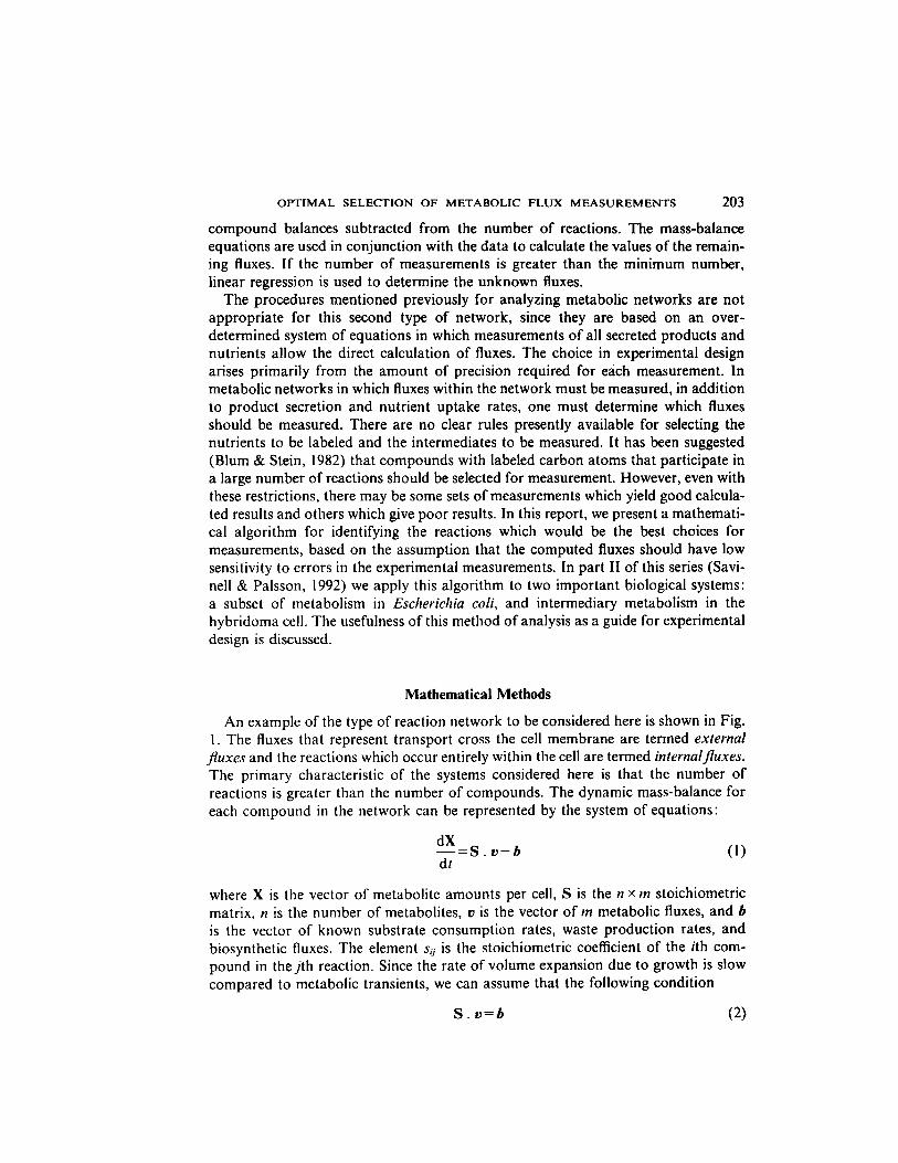
An example of the type of reaction network to be considered here is shown in Fig. 1. The fluxes that represent transport cross the cell membrane are termed external

fluxes and the reactions which occur entirely within the cell are termed internalfluxes. The primary characteristic of the systems considered here is that the number of reactions is greater than the number of compounds. The dynamic mass-balance for each compound in the network can be represented by the system of equations:

dX - s . v - b (I)

dt

where X is the vector of metabolite amounts per cell, S is the n x m stoichiometric matrix, n is the number of metabolites, v is the vector of m metabolic fluxes, and b is the vector of known substrate consumption rates, waste production rates, and biosynthetic fluxes. The element s~i is the stoichiometric coefficient of the ith com- pound in the jth reaction. Since the rate of volume expansion due to growth is slow compared to metabolic transients, we can assume that the following condition

S . o--h (2)

204 J. M. SAVINELL AND B. O. PALSSON

1 ~1 Cell memOrone

Ul 03 / / ) X I JJ

FIG. t. Example of a metabolic reaction network. Reactions td' and v2 are metabolic generation and degradation, respectively, and are termed #zternalfluxes. Reaction va involves transport across the cell membrane and is termed an externalflux. The biosynthetic demand for X~ is given by bh which is either known from the composition of the cell and the growth rate, or can be measured directly. The stoichio- metric matrix for this system has one mass balance and three fluxes, so that two of the three fluxes must be measured.

holds. Since the matrix S is known from the structure of the metabolic pathways and b is known from experimental data, this equation can be used to calculate the steady-state metabolic fluxes v.

P A R T I T I O N I N G OF F L U X E S I N T O M E A S U R E D A N D C O M P U T E D F L U X E S

In order to calculate the fluxes through the network, a minimum of (m-n) fluxes must be measured, and the remaining n fluxes calculated. The vector v and matrix S can be partitioned as follows:

v = , s = [ s c l s A

where v, are the ( m - n ) fluxes that are experimentally measured, and vc are the n fluxes to be calculated. Equation (:2) now becomes:

S~v, + S , v , = b (3)

and vc can be calculated by rearranging eqn (3):

v~ = $ 2 1 . ( b - S , v , ) . ( 4 )

Two preconditions exist for partitioning v and S. First, Sc must be non-singular, and second, the fluxes in v, must be measurable. Herein we put forth an additional criterion : the fluxes that are calculated, v~, should have low sensitivity to experimental

O P T I M A L S E L E C T I O N O F M E T A B O L I C F L U X M E A S U R E M E N T S 2 0 5

error in the measured flux values, re. This criterion can be justified as follows. If a small error in a flux measurement is magnified greatly in the calculated fluxes, the calculated solution may be very inaccurate, and therefore meaningless. On the other hand, if the calculated solution depends on the data, and yet is relatively insensitive to error in the data, then one can have confidence in the accuracy of the calculations.

Let the matrix S be appended with a p x m matrix Ip, where p = m - n , and b is appended with a p x I vector bp, where bp= re:

Fi] b, = , S, =

such that:

S, . v = b, (5) is true.

The matrix Ip is constructed such that each row in Ip will have one and only one element with value l, and the column in which the 1 is located will be designated as the kth reaction. All other elements in the row will be zero, and all other elements in the kth column will be zero. The corresponding row of bp will contain the experi- mental measurement of the kth flux. For example, for the stoichiometric matrix S corresponding to the network in Fig. l, S, may be formed such that:

SII SI2 SI3 /)1 _ _

where b2 is the measurement of flux v,, b3 is the measurement of flux v3, and v .= (v,, v~) T.

M A X I M U M S E N S I T I V I T Y T O E X P E R I M E N T A L E R R O R

The error in the data, represented by Ab,, will lead to an error in the calculations, represented by Ao. The relationship between the two, obtained from eqn (5), is:

S,. Av= Ab,. (7) The following equations are used to estimate the maximum error that can occur in the calculated fluxes.

From the property of the matrix norm (Stewart, 1973) and from eqn (5) one obtains:

llS, ll • Ilvll-> Ilb,[I. (8) Similarly, after rearranging eqn (7), one obtains:

[ I S f ' l l • IIAb, II > liAvl;. (9)

206 J. M. S A V I N E L L A N D B. O. P A L S S O N

Multiplying the terms of eqn (8) by the terms of eqn (9) and rearranging yields:

where

IIAvll IIAb, II - - < C . - (10) lit, l[ IIb, II

c = IIS, II. IIS,-'l[. (I 1) The fractional error in the calculated solution is given by IIAvll/llvll, and the

fractional error in the data is given by IIAb, ll/llt,,tl. The quantity C, termed the condition number of matrix S,, is a measure of the maximum sensitivity of the solution v to errors in the data b,. Note that C is a function only of S,. The role of the condition number in error analysis is derived and discussed thoroughly in (Wilkinson, 1963), and in many other texts on linear algebra, (e.g. Stewart, 1973).

The condition number C is thus a measure of the upper bound of the sensitivity of the calculated fluxes to error in experimental measurements in b,. In other words, C is a measure of the possible error amplification. By changing the location of the ls and 0s in lp, and calculating the condition number for each new St, one can determine the possible error amplification for each set of fluxes to be measured. In the example given above, there are three different combinations of fluxes possible, given by three different Ip:

is s2 s 1 Ei s2 i3] rs s2 s ij i i j - t o 0 ' 0 ' 1

I 0 0

where the first matrix is for v~ and vz measured, the second matrix is for vm and v3 measured, and the third matrix is for v2 and v3 measured. The best combination of fluxes to be measured is that which gives S, with the lowest condition number, and thus the lowest sensitivity to error in data. The worst choice of fluxes is given by the matrix with the highest condition number. Infinite-valued condition numbers represent flux combinations for which a computed solution is not possible.

The value of the condition number depends on the choice of norm that is used. The norm is chosen according to the type of error description that is desired. Three of the most commonly used norms are the 1-norm, the 2-norm, and the oo-norm (Stewart, 1973). When the oo-norm is used, IlAvll/llv[I represents the largest error in a single flux, normalized to the flux with the largest value (Stewart, 1973). This means of error description is not useful here and a better description is given by the 2-norm. When the 2-norm is used, IIAvll/llvfl represents the sum of all the error normalized to the sum of all the fluxes. The error description provided by the 1- norm is similar to the 2-norm. The I- and 2-norms thus are measures of the average error overall in the calculations. In this report, the condition number will be calcula- ted using the 2-norm, due to the significance of the error interpretation and the widespread use of this norm. Results using other norms may differ from those shown here, due to the difference in error interpretation.

O P T I M A L S E L E C T I O N O F M E T A B O L I C F L U X M E A S U R E M E N T S

The 2-norms of S, and S,- i are given by (Strang, 1980) :

IIS, II = 6.

1 IIS,- ' II cr 0

where 6- and cr ° are the maximum and minimum singular values of S,, respectively. The condition number C can then be calculated by:

6" C - (12)

o- 0

207

A C T U A L S E N S I T I V I T Y T O E X P E R I M E N T A L E R R O R

The value of C obtained from eqn (i 2) is only an upper bound on the sensitivity. Because this is an upper bound, a set of fluxes with a high condition number has the potential to result in a more sensitive solution than the low-condition number set, although the high-condition number set will not necessarily be more sensitive than the low-condition number set. The actual sensitivity, R, of the calculated fluxes to the experimental data is defined by:

IIAvll IIAb, tl - R . - - ( 1 3 )

IIvll IIb, ll

where R must always be less than or equal to C. The actual sensitivity, R, is a function not only of St, but also of the values of the experimental measurements and the error, given by b, and Abt, respectively.

The condition for R = C occurs when the inequalities in eqns (8) and (9) become equalities. The vectors b, . . . . . Ab, ...... vm~, and Avmax, which satisfy these equalities are defined by:

[Is,II • [lv~o~[l = lib, . . . . II ( 1 4 )

IIS7'11. IIAb,., . ,~ll = IIAv,.°=ll. ( 1 5 )

The values of bt and Ab, are obtained by the singular value decomposition of St and St- i By the singular value decomposition theorem, S, can be decomposed as (Strang, 1980) :

S, = UIBW r

where ]B is a diagonal matrix, with each element along the diagonal called a singular value, and U and W are orthonormal matrices.

It is shown in the Appendix that a sufficient condition for eqn (14) to be true is when :

b, . . . . = a S , ~ (16 )

b~

> b 2

~ o

0.6

0 - 4 -

0 . 2 -

0-050 '

(b

/ @ : 8 0

i I I i [ I I I I I I I I I i I I 0 50 I00

# 150

0.6

0 . 4

0.2

( c )

I t 0 50 I00 150

8

FIG. 2. (a) Illustration of the angles 0 and ~b for the example system in Fig. I. The biosynthetic demands and flux measurements are represented by b, and Ab, represents the error in the measurements. The vectors b,~,,.~ and Ab ..... . given by eqns (16) and (17), result in R = C. The value of the biosynthetic demand, bt, is set to 7 and the value of the error in biosynthetic demand, Abe, is set to 6. The projection of b, and Ab, onto the plane [b , ( l )= y] is shown and 0 is the angle between these projections. Similarly, the projection of &b, and Ab,~,x onto the plane [Ab,(I) = 5 ] is shown and ~b is the angle between these projections. (b) The value of sensitivity/condition number as a function of the angle q~ between the projections of Ab, and Ab, . . . . onto the plane [b, ( l )=0] for the system given by eqn (18). The angle between the projections of b, and b . . . . onto the plane [b,(I ) =0] is given by 0. (c) The value of sensitivity/ condition number as a function of 0 when ~b=0.

O P T I M A L SELECTION OF M E T A B O L I C FLUX M E A S U R E M E N T S 2 0 9

The parameter a is any scalar value, and ~ is the column of W that corresponds to the maximum singular value of S,. Similarly, eqn (15) is true when:

At,,.,,,~ =/~,, ° (17)

where u ° is the column of U that corresponds to the minimum value in lz and fl is any scalar value. Thus, the directions of bt and Ab, for which R is exactly equal to C, are given by eqns (16) and (17).

The influence of b, and Ab, on R is illustrated by means of the example system illustrated in Fig. 1, where S, is given by:

S, = 0 (18) 0

and b, is a 3 x 1 vector. The first element of b, is the biosynthetic demand, with the value b~, and the error in this demand, Ab,, has the value Abe. All possible directions of b, and Ab,, with the restriction that b,(1) = b~ and Ab,(l) = Abl, can be considered by independently varying the value of the second element of each vector and calculat- ing the third element, keeping the magnitudes constant. The actual sensitivity, R, is calculated for each b, and Ab, using eqn (13), and R is plotted as a function of two angles ~b and 0. As illustrated in Fig. 2(a), ~b is the angle between the projections of Ab, and Ab, ..... in the plane of Ab,(1) = Abt, and 0 is the angle between the projections of b, and b, ..... in the plane of b,( l)=bj .

Figure 2(b) and (c) illustrates that both ~b and 0 influence the sensitivity. Although the maximum theoretical value of R/C is 1, this value will rarely occur in a biological system. The reason that R/C is small is that the values of Ab, ..... and b, ..... are given by the singular value decomposition of St, and thus most elements of these vectors are non-zero. However, many of the biosynthetic fluxes in b, have zero values, since not all metabolites are involved in biosynthesis. Hence, the physiological Abt and bt will always be displaced from Ab, ..... and b, . . . . . causing R to be less than C. Figure 2(b) and (c) demonstrates, for this example, that the condition number will always overestimate the actual sensitivity by at least a factor of 2, regardless of the values of the flux measurements and the measurement error. When systems with larger dimension are considered, the maximum value of the ratio R/C tends to decrease. However, as will be shown later, there is a correlation between the sensitivity R obtained using an estimate of b, and the condition number. Consequently, the condi- tion number can be used to estimate relative sensitivities between flux arrangements, even though the actual sensitivity may be much less than that given by the condition number.

E F F E C T OF E R R O R D I R E C T I O N

The values of/1, are characteristic of the system and the environment, while the values of Ab, are determined by the precision of the instruments and techniques used in measurement. Conseqently, the values of Ab, are essentially unknown. Since the

210 J. M. SAVINELL AND B. O. PALSSON

elements of Ab, represent errors in measurement that are mostly independent, the vector Ab, can theoretically have any direction in (m-n) dimensional space. The magnitude of Ab, can be considered to be constant, since the magnitudes of Ab, and Av cancel in eqn (13). Thus, all possible directions of Ab, can be thought to be represented by all points on the surface of a sphere in (m-n)-dimensional space.

Figure 3(a) illustrates the surface traced by Abt for the example system given by eqn (6). In this example the surface is a circle because only two measurements ( m - n = 2 ) are needed. An even distribution of points on this surface is needed in order to determine the effect of the direction of the error vector, represented by each point, on the sensitivity. Each element of Ab, is assigned a random value, and the vector magnitude is calculated. All vectors with magnitude greater than 1 are dis- carded, and those with magnitude less than or equal to 1 are normalized to I, thus ensuring an even distribution of points. The sensitivity of the computed solution to the measured solution, for a particular experimental design given by S,, can be calculated for each of these remaining error vectors. Since the objective is to deter- mine the most probable sensitivity when the measurement error is unknown, a fre- quency distribution is obtained from the calculated sensitivities, as shown in Fig.

b~ Ab3 ( o ) ~ L~b2

(b)

FIG. 3. (a) Illustration of the surface traced by all possible directions of Ab,, for the example system given by eqn (6). Since only two fluxes must be measured for this example, the surface in this example is a circle in two-dimensional space. (b) A hypothetical frequency distribution of the actual sensitivities, R, calculated for each Ab,, where /~ represents the most probable sensitivity.

3(b). The maximum value of this curve represents the most probable value of R. This procedure will be illustrated in detail using two biological models in part II of this series (Savinell & Palsson, 1992).

EFFECT OF ADDITIONAL MEASUREMENTS

The analysis presented above has assumed that only the minimum number of fluxes would be measured. In many instances, a greater number of fluxes are measured, in order to check for the consistency of the data and the accuracy of the metabolic network. If the number of fluxes measured is greater than m - n , the appended stoichiometric matrix is no longer square and is designated by S~, where 17 represents the number of additional measurements. The resulting set of mass balances is thus

OPTIMAL SELECTION OF METABOLIC FLUX MEASUREMENTS 211

an overdetermined set of possibly inconsistent equations, where the best estimate of the fluxes, 0, are calculated using linear regression:

STrS",O=STrb,. (19)

This method of solution is discussed in most linear algebra texts (e.g. Strang, 1980). From eqn (19) one can derive:

IIA011 IISTrAb, II < C , . - - (20) 11011 - IIS,"rb, II

where

C, = IISTTSTII. II(STTS~)-'II. (21)

In this derivation of sensitivity, the error vector and the measurement vector are multiplied by $7 r, so that the interpretation of C~ is somewhat different from the interpretation of C. To compare the maximum possible sensitivity using excess meas- urements with the minimum number of measurements, we note that when 1/= 0, i.e. $7 = S,, then

Co = IlS,rS, II. ll(S,rS,)-'ll = C 2

is true. The value of C, is calculated for 17 = 0, 1, 2 , . . . , m - (m - n) for the example systems in part II (Savinell & Paisson, 1992).

The actual sensitivity of the computed solution when excess flux measurements are made, R~, is defined analogous to eqn (20):

IIAell IIS,"TAb, II • - - . ( 2 2 )

11011-R, iiS,,Tb, ii

In order to calculate the upper bound on R,, the following expression is used, analogous to eqn (17) :

S,°rAb,.~, = flu ° (23)

where u ° is the column of U corresponding to the smallest singular value of the matrix S~rS~.

D i s c u s s i o n

The estimation of steady-state fluxes in a biochemical network is usually obtained by measuring some of the fluxes, and using the mass-balance equations to compute the other fluxes. An algorithm is derived for estimating the sensitivity of the computed fluxes to experimental error in the measured fluxes. The upper bound on this sensitiv- ity is given by the condition number, which is a function only of stoichiometry. If estimates of the fluxes are available before the experiment is performed, then a more realistic sensitivity can be calculated. The experiment is then designed such that the combination of fluxes which yield low sensitivity is selected for measurement. This

2 1 2 J . M . S A V I N E L L A N D B. O. P A L S S O N

algorithm will be illustrated with two model systems, E. colt and a hybridoma cell line, in part II o f this series.

This research was supported by National Science Foundation grant BCS-9009389. The authors thank James S. Freudenberg for his help with the derivation in the Appendix.

REFERENCES

BLACKWOOD, A., NEISH, A. & LEDINGHAM, G. (1956). Dissimilation of glucose at controlled pH values by pigmented and non-pigmented strains of Escherichia colt. J. Bact. 72, 497.

BLUM, J. J. & STEIN, R. B. (1982). On the analysis of metabolic networks. In Biological Regulation and Development Vol. 3A (Goldberger, R. & Yamamoto, K., eds) pp. 99-125. New York: Plenum Press.

CRAWFORD, J. M. t~. BLUM, J. J. (1983). Quantitative analysis of flux along the gluconeogenic, glycolytic and pentose phosphate pathways under reducing conditions in hepatocytes isolated from fed rats. Biochem. J. 212, 595-598.

ERICKSON, L., SELGA, S. • VIESTURS, U. (1978). Application of mass and energy balances regularities to product formation. Biotechnol. Bioengng. 20, 1623.

NIRANJAN, S. ~£ SAN, K.-Y. (1989). Analysis of a framework using material balances in metabolic pathways to elucidate cellular metabolism. Bioteehnol. Bioengng. 34, 496-501.

PAPOUTSAKIS, E. T. & MEYER, C. L. (1985). Equations and calculations of product yields and preferred pathways for butanediol and mixed-acid fermentations. Biotecbnol. Bioengng. 27, 50-66.

RAnKm, M. & BLUM, J. (1985). Quantitative analysis of intermediary metabolism in hepatocytes incuba- ted in the presence and absence of glucagon with a substrate mixture containing glucose, ribose, fructose, alanine and acetate. Biochem. J. 225, 761-786.

SAFER, B. 8£ WILLIAMSON, J. (1973). Mitochondrial and cytosolic interactions in perfused rat heart. Role of coupled transamination in repletion of citric acid cycle intermediates. J. biol. Chem. 248(7), 2570-2579.

SAUER, F., ER1--LE, J. & BINNS, M. (1970). Turnover rates and intracellular pool size distribution of citrate cycle intermediates in normal, diabetic and fat-fed rats estimated by computer analysis from specific activity decay data of ~4C-labeled citrate cycle acids. Eur. J. Biocbem., 17, 350-363.

SAVINELL, J. M. & PAt.SSON, B. O. (1992). Optimal selection of metabolic fluxes for in vivo measurement. II. Application to Escherichia Colt and hybridoma cell metabolism. J. theor. Biol. 155, 215-241.

STEm, R. B. & BLUM, J. (1979). Quantitative analysis of intermediary metabolism in tetrahymena pj'riforntis; cells grown in proteose-peptone and resuspended in a defined nutrient-rich medium. J. biol. Chem. 254(20), 10385-10395.

STERN, R. B. & Bt.UM, J. (1980). Quantitative analysis of intermediary metabolism in tetrahymena puriformis; cells grown in glucose-supplemented medium. J. biol. Chem. 255(9), 4198~1205.

STEWN, R. B. & BLUM, J. (1981). Quantitative analysis of intermediary metabolism in tetrahymena pyriformis; cells kept under static conditions for four hours after growth in glucose-supplemented medium. J. biol. Chem. 256(6), 2752-2760.

STEWART, G. (1973). hmoduction to Matrix Computations. London: Academic Press. STRANG, G. (1980). Lh~ear Algebra and its Applications. London : Academic Press. STUCK I, J. W. & WALTEr',, P. (1972). Pyruvate metabolism in mitochondria from rat liver: measured and

computer-simulated fluxes. Eur. J. Biochem. 30, 60-72. TSAI, S. & LEE, Y. (1988). Application of Gibbs' rule and a simple pathway method to microbial

stoichiometry. Biotechnol. Prog. 4(2), 82-88. VALL1NO, J. J. & STEPHANOPOULOS, G. (1989). Flux determination in cellular bioreaction networks:

applications to lysine fermentations. In: Frontiers in Bioprocessing (Sikdar, S. K., Bier, M. & Todd, P., eds) pp. 205-219. Boca Raton, FL: CRC Press.

W,LKmSON, J. (1963). Rounding Errors in Algebraic Processes. Englewood Cliffs, N J: Prentice-Hall.

APPENDIX

Derivation of Conditions for R = C

T h e o b j e c t i v e o f this p r o o f is to s h o w t h a t the e x p r e s s i o n fo r Ab, . . . . g iven by e q n (16) is a suff ic ient c o n d i t i o n fo r eqn (14) to be t rue. B e f o r e p r e s e n t i n g the p r o o f we

OPTIMAL SELECTION OF METABOLIC FLUX MEASUREMENTS 213

note that the rearrangement of eqns (5) and (14) yields:

IIS,v., .~ll = IlS,II • IIo=.~ll = IIb , , ,~ l l . ( g . l )

The singular value decomposition (SVD) of S, is given by:

S, = UEW r = Ztraiw r. (A.2)

Since U and W r are orthonormal matrices (by the SVD theorem), the following can be obtained from eqn (A.2):

S,W = UE (A.3)

S,wi = cr,~i. (A.4)

Let O be the largest singular value of St, and ti and • be the corresponding columns of U and W, respectively. From the definition of the 2-norm, and using the SVD theorem, one can derive the following (Strang, 1980):

lISA = O. (m.5)

Further, since U and W r are orthonormal matrices, the following is true:

Iluill = IIw, II = 1. (m.6)

We begin the proof by assuming that v,~.., is given by:

v,,,,x = a • (A.7)

and thus

b,.max = S,v,~.# = aSia.

Combining eqns (A.4) and (A.8), we obtain:

S t v , , , a x = ot 0~.

Using eqn (29), we obtain from eqn (A.9):

l [S ,v . , .x 1} = a e .

Inserting eqn (28) into the previous equation gives:

l is ,t , , , . . , l l = a IIS, ll.

From eqns (A.6) and (A.7):

(A.8)

(A.9)

( A . 1 o )

and inserting this expression for a into eqn (A.10) gives

IlS, v,.°..ll = IIS, II. I Iv . , .A = IIb,~.~ll ( m . 1 2 )

which is eqn (A. 1). Therefore, b,..,.~ = aS,~ is a sufficient condition for eqn (I4) to be true.

llVm,~l[=a (A.II)

2 1 4 J, M. SAVINELL AND B. O. PALSSON

The derivation of the expression for Ab,.,,,~ given by eqn (17), which must satisfy eqn (15), proceeds along similar lines. The singular value decomposition of S, -I is given by:

S, -I = W~='U r. (A.13)

It can be shown, by analogy with the above derivation, that

Ab,.m,~ = f lu ° (A. 14)

where u ° is the column of U corresponding to the maximum value of r.-i . The maximum value of ~ - ' corresponds to the minimum singular value of r.. Thus, u °

corresponds to the minimum singular value of St. It can also be proven that Ab,.,,~ is orthogonal to b,.,,~, as illustrated in Fig. 2.