nutation damping theory and computer implementation - tu/e

NUTATION DAMPING

THEORY

AND

COMPUTER IMPLEMENTATION

Author: C. van Bake1 id.nr. : 252829 mentor UCN: S. Kermans mentor TUE: A. de Kraker WFW document: WFW 93.006

UCN, Almelo, January 1993

Abstract 2

Abstract

The movement of spinning satellites is often disturbed by nutationally and antenna movement induced motions. These (unwanted) motions have to be damped and a tube-with-endpots damper can be used for this purpose. At UCN Almelo the nutation damping theory for the tube with

endpots damper was spread about many different reports. In this report all the theory necessary for the design of a tube with endpots damper is collected. Expressions are given for the fluid displacement in the

endpots, the fluid velocity in the fluid tube and the damper performance. In order to test the damper on earth, scaling is necessary. The scaling relations are derived for this purpose. The computer implementation of the theoretical model Is described. Results were calculated for a practical model. These results

were compared with test results and an accurate agreement was found for small nutation angles. The model is found to be inaccurate for large nutation angles. Therefore an update of the theory is recommended.

Symbols 3

SMibOlS

Em1 a Tube radius of damper

aO Amplitude of forcimg acceleration Cm/s21

beginning of a testrun 6m/s21

a- Forcing acceleration along the fluid tube at the

Forcing acceleration along the fluid tube at the end of a testrun Centrifugal acceleration of the rotor of the testing apparatus Acceleration as a result of the spin velocity of the damper on the satellite Tangential acceleration of the rotor of the testing apparatus Forcing acceleration Endpot radius of damper Effective endpot radius in case of testing a flight model Constant defining the relation between a,, and s distance between outer radii of fluid tube and vapour tube Frequency ratio n/o, Radius dependent fluid velocity Amplitude of tube-wall velocity Gravity Equivalent for the gravitational force on the fluid Torsional stiffness of the rotor of the testing apparatus Mean height fluid level Effective mean height fluid level in case of testing a flight model Moment of inertia of the rotor of the testing apparatus Moment of inertia with respect to i-axis Tube length of damper

Angular momentum axis of satellite

Em1 [ Nm/rad ]

Cm1

Symbols 4

Effective tube length of damper [ml Scale factor [-I Mass C W I

[-I Power r J/sl

Radius [ml

Match factor for fluid surface tilt

Principal axis of satellite

Mounting radius of damper (distance from spin-axis to centre of fluid tube) Mounting radius of PTM's on rotor of the testing apparatus fluid displacement in endpot Effective fluid displacement in endpot in case of testing a flight model Time Pendulum time Estimated duration of a testrun Radius and time-dependent fluid velocity Match factor for effective tube length Tilt angle of the flight model Twist of the rotor of the testing apparatus Top angle of body cone of satellite Nutation angle initial nutation angle Dynamic viscosity of damping fluid Kinematic viscosity of damping fluid Density of damping fluid Time constant Angular deviation of the rotor of the testing apparatus Angular deviation of the rotor at the beginning of a testrun Angular deviation of the rotor at the end of a testrun instantaneous rotation axis of satellite Natural damper frequency frequency of the rotor of the testing

Symbols 5

apparatus [rad/sI o, Spin frequency Crad/sI n Nutation frequency [rad/sl

Contents 6

Abstract . . . . e . . . . . . . . . . . . . . . . . . . 2

Symbols . . . . . e . . . . . . . . . . . . . . . . . . . 3

1. Introduction o e e 6 e 6 i o e 6 e 5 i o 5 i i o i e 8

2. Satellite motion . . . . . . . . . . . . . . . . . . . 9

2.1. Satellite nutation . . . . . . . . . . . . . . . . 9

2.2. Satellite motion due to antenna movement . . . . . 11

3. Nutation damping e e e e . e e . e a e e . . e . . 13

3.1. Why nutation damping? . . . . . . . . . . . . . . 13

3.2. History of nutation dampers . . . . . . . . . . . 13

4. Nutation damper . . . . . . . . . . . . . . . . . . 4.1. Introduction . . . . . . . . . . . . . . . . . .

4.1.1. Oblate versus prolate spacecrafts . . . . . 4.1.2. The coupling between satellite and damper . 4.1.3. Equatorial versus meridional configuration 4.1.4. Tube-with-endpots damper . . . . . e . . .

4.2. Time constant . . . . . . . . . . . . . . . . . 4.3. Performance theory . . . . . . . . . . . . . . .

4.3.1. Elaboration Fokker . . . . . . . . . . . . 4.3.2. Elaboration ESA . . . . . . . . . . . . . . 4.3.3. Comparison of the Fokker elaboration versus

ESA elaboration . . . . . . . . . . . . e . 4.4. Simultaneous excitations . . . . . . . . . . . . 4.5. Effective tube length . . . . . . . . . . . . . 4.6. Fluid surface tilt . . . . . . . . . . . . . . . 4.7. Matching the theory with practice . . . . . . . 4.8. Conclusion . . . . . . . . . . . . . . . . . . .

% 14 14

14

14

16

16

17 18

19

20

the 20

21

22

23

24

25

5. Performance tests . . . . . . . . . . . . . . . . . . 26

5.1. Introduction . . . . . . . . . . . . . . . . . . . 26

5.2. Test facility . . . . . . . . . . . . . . e . . . 26

5.2.1. Test equipment . . . . . . . . . . . . . . . 26

Contents

5.2.2. Test procedure . . . . . . . . . . . . . . . 5.3. Definition of the performance test models . . .

5.3.1. Scaling . . . . . . . . . . . . . . . . . . . 5.3.2. Scaling relations . . . . . . . . . . . . . . 5.3.3. Testing apparatus performance calculations .

5.4. Test set-up analysis . . . . . . . . . . . . . . . 5.4.1 Minimum duration of a testrun . . . . . . . . 5.4.2. Torsional stability of the rotor . . . . . . 5.4.3. Mounting radius range . . . . . . . . . . . .

5.5. Testing a flight model . . . . . . . . . . . . . .

6 . Computer implementation . . . . . . . . . . . . . . . 6.1. Introduction . . . . . . . . . . . . . . . . . . . 6.2. Software package . . . . . . . . . . . . . . . . .

6.2.1. units . . . . . . . . . . . . . . . . . . . . 6.2.2. Program . . . . . . . . . . . . . . . . . . . 6.2.3. Input . . . . . . . . . . . . . . . . . . . . 6.2.4. Output . . . . . . . . . . . . . . . . . . .

6.3. Software check . . . . . . . . . . . . . . . . . .

7 . Conclusion and recommendations . . . . . . . . . . . .

8 . Literature . . . . . . . . . . . . . . . . . . . . . .

7

26

27

27

27

28

28

28

29

29

30

31

31

31

31

31

32

32

33

35

36

Appendix A: Design example Appendix B: Pascal inputfiles

Introduction 8

1. Introduction

At UCN tube-with-endpots nutation dampers are designed and made. In order to be able to design such a damper, software has been developed for the necessary calculations. The theory behind the software was spread about many different reports. For further applications, it is more converiient t h a t a i l the necessary information is found in one report.

damper for single spin satellites. No derivation of the satellite equations of motion will be given. All parameters which follow directly from these equations of motion will be considered postulated. This report is a collection of the theory. It contains a

description of the software and gives an example on h o w to design a nutation damper including the test-model.

separate report [12].

This report is oriented to one kind of passive type nutation

The derivations of the damper theory are all printed in a

Satellite motion 9

2. satellite motion

2.1. Satellite nutation The attitude motion of a completely rigid, rotating object

in space free of all external forces or torques is considered. In describing this motion! four fundamental axes or sets of axes are important [ 4 ] .

Geometrical axes are arbitrarily defined relative to the structure of the spacecraft itself. This is the reference system which defines the orientation of the satellite in

inertial space. The angular momentum axis i is the axis through the centre of mass parallel to the angular momentum vector. The instantaneous rotation axis W is the axis about which the spacecraft is rotating at any instant. The principal

axis is any axis P such that the resulting angular momentum is parallel to P when the spacecraft rotates about P . These four sets of axes may be used to define two types of

attitude motion called pure rotation and nutation (fig i ) .

Ir1 P U R E ROTATION

- IC) NUTATION

I

F i g u r e 1: two t y p e s of a t t i t u d e motion

Pure rotation is the case in which the rotation axis, a principal axis, a geometrical axis and the angular momentum vector are all parallel or anti-parallel (fig i(a)). These four axes will remain parallel as the object rotates.

rotation axis is not aligned with a principal axis Nutation is rotational motion for which the instantaneous

(fig i ( c ) ) .

Satellite motion 10

In this case, the angular momentum vector, which remains fixed in space, will not be aligned with either of the other

physical axes. Both P and W rotate about x. P is fixed in the spacecraft. Neither i nor W is fixed in the spacecraft. ij rotates both in the spacecraft and in inertial space, while L rotates in the spacecraft, but is fixeu in inertial space. The

angle between P and i!, is a measure of the magnitude of the

nutation, called the nutation angle, 8. To obtain a physical feel for nutation, it is noted that in

inertial space, ij rotates about J!, on a cone of half-cone angle ( [ - O ) called the space cone, as illustrated in figure 2 (left) for I,>13. Similarly, W maintains a fixed angle, r, with P and, therefore, rotates about P on a cone called the body cone. Because 0 is the instantaneous rotation axis, the body is

instantaneous at rest along the ij axis as ij moves about z. Therefore, we may visualize the motion of the spacecraft as

the body cone rolling without slipping on the space cone (see figure 2).

I

F i g u r e 2 : Motion of a n u t a t i n g s p a c e c r a f t , the body cone ro l l s on the space cone f o r 11=12>13 ( l e f t ) and 11=12<13 ( r i g h t )

Satellite motion 11

The space cone is fixed in space and the body cone is fixed in the spacecraft. Figure 2 left is correct only for objects, such as a tall cylinder, for which I, is greater than I,. If I, is greater than I,, as in the case of a thin disk, the space cone lies inside the body cone, as shown in figure 2 right.

2.2. Satellite motion due to antenna movement A satellite can have another nutation-like motion. This

motion is caused by the movement of antennas. When a satellite is positioned, the antennas will oscillate due to their moment of inertia and their flexibility. This oscillation of the antennas will cause the satellite to oscillate. Various modes of antenna movement of a satellite with four antennas are illustrated in figure 3 [ll].

The symmetric antenna mode will not cause the satellite to oscillate unlike the antisymmetric antenna mode. So the frequency of this latter mode will be important to design the damper.

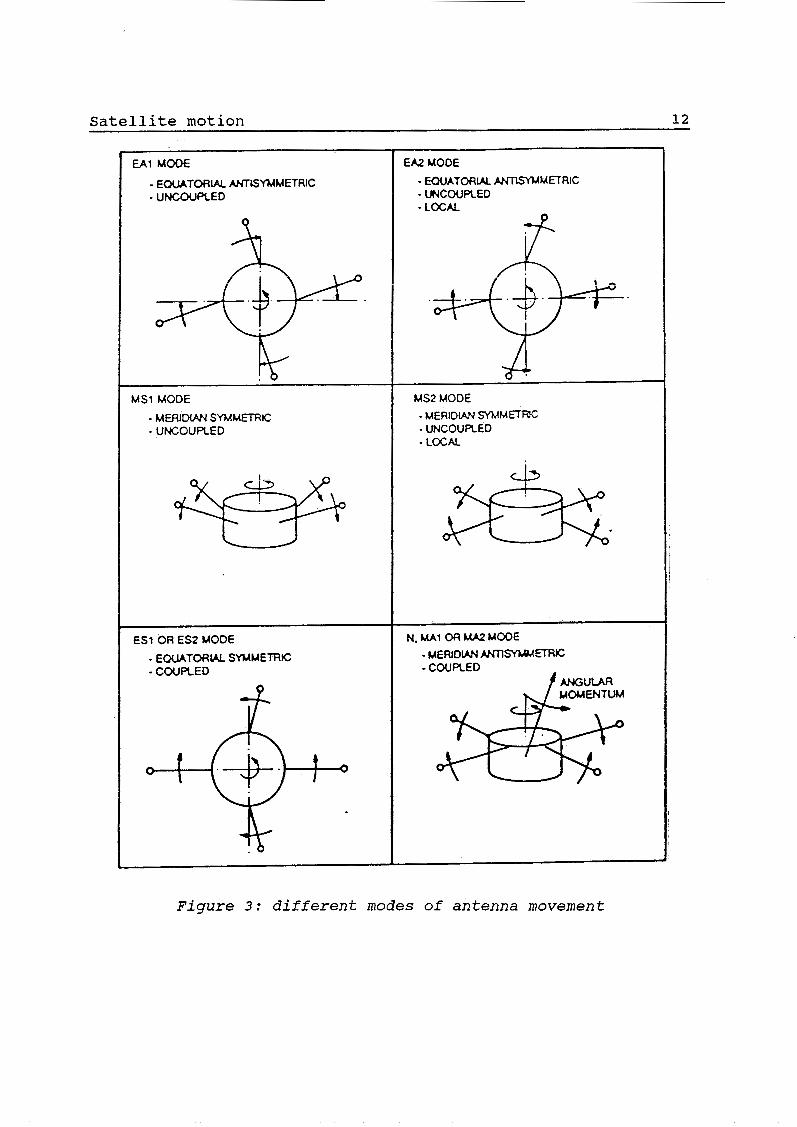
Satellite motion 12

EA1 M O M - EQUATORIAL ANTSYMMETRIC - UNCOUPLED

MS1 MODE - MERIMAN SYMMETRC - UNCOUPLED

- EQUATORLAL SYMMETRK; - COUPLED

EA2 MODE

- MUATORUL ANTLWJMEIRIC - UNCOUPLED - LOCAL

MS2 MODE - MERIOiAN W M m - UNCOUPLED - LOCAL

Figure 3: d i f f e r e n t modes o f antenna movement

Nutation dampinq 13

3. Nutation dampins r l l

3.1. Why nutation dampins? One method to stabilize the attitude of a satellite in

space, is by giving it a rotational movement around the spin- axis. With this rotational movement the satellite gains a gyroscopic stiffness which allows it to be controlled accurately. Since observational instruments need to be aligned to the spin-axis or positioned under a certain angle with this axis for scanning purposes, any unwanted oscillations caused by attitude and orbit control need to be damped out. Therefore such a satellite is equipped with one or more nutation dampers.

3.2. History of nutation dampers Nutation dampers were first developed for the stabilization

of aircraft gyroscopes. Further work on nutation dampers was done for spin-stabilized rockets that were propelled beyond the earth atmosphere where fin stabilization becomes ineffec- tive because of the absence of air. The first nutation damper flown in a missile was built at the Naval Ordnance Test Station, U.S.A., in 1950 for the stabilization of the gyros- cope in the Sidewinder missile. This damper consisted of an annular damper that was partially filled with mercury. The sloshing of the mercury dissipated the nutational energy. A

similar mercury filled annular damper was used in the Pioneer- I lunar probe in 1958 and became the first nutation damper to be used in space. Since then many types of nutation dampers have been designed

for spin-stabilized spacecrafts ranging in size from small scientific satellites to large communication satellites. Although communication satellites are generally 3-axis stabilized in geostationary orbit, they are spin-stabilized during their transfer orbit.

Nutation damper 14 ~~

4, Nutation damper

4.1. Introduction 4.1.1, Oblate versus prslate spacecrafts

spacecrafts. The spacecraft is oblate and stable, if the spacecraft has a nominal spin-axis which is the principal axis with maximal moment of inertia. Otherwise the spacecraft is prolate and unstable. When energy is dissipated, the angular momentum vector

becomes aligned with the principal axis with the largest moment of inertia. So if a passive nutation damper is used on a prolate spacecraft, the nutation angle will increase as a result of the energy dissipation. The solution for this problem is the use of an active nutation uamper [43.

A distinction has to be made between oblate and prolate

I

F i g u r e 4 : T h i s s p a c e c r a f t i s p r o l a t e because the nominal s p i n a x i s P, i s the a x i s w i t h minimum moment of i n e r t i a

4 .1 .2 . The coupling between satellite and damper In this paragraph a short note will be given on the coupling

Because the damper mass is small in comparison to the between satellite and damper.

satellite mass, the solution of the equations of motion can be simplified by neglecting the effect of the moving damper mass

Nutation damper 15

on the motion of the satellite body. The motion of the satellite is then decoupled from the motion of the damper mass. The satellite equation of motion can now be solved separately from the damper equation of motion.

r i g i d body motion

change of a v e r a g e d e n e r g y n u t a t i o n a l d i s s i p a t i o n

o v e r 1 n u t a t i o n e n e r g y c y c l e

4

e n e r g y of sa te l l i t e

i

n u t a t i o n a n g l e t i m e h i s t o r y

*

+ periodic

f o r c i n g accele- r a t i o n o n damper mass

damper e q u a t i o n of mot ion

I

Figure 5: The energy sink method

With the satellite equations of motion, the nutational energy is calculated as well as the periodic forcing acceleration on the damper mass. The energy, which is dissipated in the damper during one nutation cycle, is calculated by substitution of the forcing acceleration in the damper equation of motion. In this calculation the forcing acceleration is assumed to remain constant. Now the over one cycle averaged dissipated energy is subtracted from the total.

Nutation damper 16

energy to obtain the nutational energy after one (dissipated) nutation cycle.

ically shown in figure 5. This method is only valid if the nutational cycle time is small in comparison to the total dampina time. If the nutation frequency is small, the cycle time will be large and the energy sink method will not be valid.

This method is called the energy sink method and is schemat-

4.1.3. Equatorial versus meridional configuration

equatorial and meridional (figure 6). The tube of the equatorial damper is curved with the centre of curvature on the spin-axis due to the curvature of the acceleration field 113.

The damper can be mounted in two different configurations:

!s n

2: <

Y / ~ - - - - - / - \ L ~ ~ ~ I p *

---- ----- \&'

x

x F i g u r e 6 : e q u a t o r i a l l y ( l e f t ) and m e r i d i o n a l l y ( r i g h t )

mounted damper

4.1.4. Tube-with-endpots damper

connected by two tubes (figure 7). The damper is located on the satellite such that oscillatory nutational motion produces an acceleration component along the damping tube. This causes the fluid to move in the lower tube (denoted as fluid tube)

The tube-with-endpots damper consists of two endpots

Nutation damper 17

and viscous friction in the fluid converts mechanical energy into heat. This energy conversion provides the damping action [5]. The gas (upper) tube guarantees fluid movement without pressure raise in the gas above the fluid. Required is that no fluid will enter this vapour tube.

vapour tube

f i g u r e 7 : Schemat i c drawing of a t u b e w i t h e n d p o t s damper

One of the advantages of this damper is its almost zero dead-band. This means damping will occur until nutation angles close to zero are reached. The damping performance is measured by the power dissipation

normalized with the amplitude of the forcing acceleration (P/a:). This performance is a function of the frequency of the forcing acceleration and shows an extreme at its resonance frequency. In general the damper will be designed such that its resonance frequency is close to the middle of the range of expected forcing frequencies.

4.2. Time constant The decay of the nutation angle can be characterized by its

time constant. This time constant can be established unam-

Nutation damper 18

biguously if the nutation angle changes exponentially with time. It is defined as the time in which the nutation angle has changed with a predefined factor.

of 8 can be described with: In the area of small nutation angles €3, the time dependence

t -- 8 i t i =6,e ' ( 4 . i)

in which I is the time-constant. The time-constant is calculated with [l]:

where P is a function, which depends on the geometry of the satellite and the mounting configuration (equatorial or meridional) of the damper. This function is not damper-dependent and its derivation is beyond the scope of this report, for this one is referred to [l], [2] and [3].

(4.2). (P/a:) is called the performance of the damper. The time-constant is dependent on (P/a:) as can be seen from

4.3. Performance theorv i 7 1

In order to be able to derive a formula for the damperperformance, the next assumptions are made: The fluid is incompressible; The fluid is isoviscous; The flow is laminar and parallel to the z-axis of the tube (length-axis) ;

A steady state response is regarded; The acceleration field is harmonic; Entrance/exit effects of the fluid in the endpots are neglected; The energy dissipation in the endpots is neglected.

Two different elaborations of the same model have been developed by Fokker and ESA. The first part of both elaborations are basically the same, but some different steps are made in the last parts of the two elaborations. Both elabo-

Nutation damper 19

rations are described completely in [12]. Below a qualitative description is given of both models with some important results.

Both models are based upon the Navier-Stokes equation. A

parameter transformation a Bessel equation of order zero is derived. This Bessel equation has a standard solution. From this point the elaborations of Fokker and ESA differ.

soiutisn is derived by separation of variables. With a

4.3.1. Elaboration Fokker Fokker describes the fluid velocity. With the matching

boundary condition, the fluid velocity as a function of time and radius is derived [12]:

[In/ SI (4-3)

E a = a , í m and r=r,í-.

in which wo is the resonance frequency of the damper.

derived using the real part of the velocity. This results in the next equation:

Next a formula for the power dissipation of the damper is

[kg. SI ( 4 - 4 )

r a with e=-, and o=-. a V

This is an equation for the power dissipation averaged over one cycle. An expression for the fluid displacement is derived inte-

grating the fluid velocity. The expression for the amplitude of the fluid displacement is:

Nutation damper 20

This amplitude, which represents the maximum fluid displacement in the endpot, is of importance for the calculation of the distance between the fluid-tube and the vapour-tube.

4.3.2. Elaboration ESA ESA describes the absolute fluid velocity. With the accor-

ding boundary condition, the fluid velocity as a function of time and radius is derived as [12]:

The formula for the power dissipation is derived using the formula for the fluid velocity. The integral over the tube area is transformed into the integral over the wall by utilizing the theorem of Stokes. This results for the power dissipation:

ESA didn't derive an equation for the fluid displacement.

4.3.3. Comparison of the Fokker elaboration versus the ESA elaboration Fokker describes the fluid-velocity relative to the fluid

tube whereas ESA describes the absolute velocity, but this difference is only expressed in the reference system in which all variables are described. A different reference system doesn't have any influence on the power-dissipation.

with respect to the tube radius, where ESA calculates the power-dissipation with a boundary condition for the fluid velocity. Both models give a different expression €or the damper-

performance, but because the models are based on the same

Fokker calculates the power-dissipation with an integral

Nutation damper 21

theory, the two expressions should calculate the same results. The softwarecheck of the computerprograms show that the models calculate equal results (see chapter 6.3).

4 . 4 . Simultaneous excitations In this paragraph the model is extended to simultaneous

harmonic excitations. Such a state of composed motion may occur in space, in case antenna modes and nutation modes are acting at the same time. For instance, at the early opera- tional phase directly after the antenna deployment. The different acceleration fields of each motion may simply be superimposed. In [12] the theoretical derivations are reported.

Fokker. A superposition of different acceleration fields is executed. These acceleration fields differ in amplitude and in frequency. The dissipated power is calculated as a function of time, because the energy sink method is not valid for all cases. When two accelerations with almost equal cycle times act simultaneously, the resulting cycle time can become large in comparison to the total damping time. So the power dissipation is not averaged over one cycle. The next equation results :

The extension of the model uses the elaboration according to

In this equation n is the number of different excitations. P i j ( < > =c&) +c&> +C,i(S) +C,,(<>

P, is the dissipated power for simultaneous excitations with excitation i and j.

Nutation damper 22

.--- , < b >

/ --. L 'I4

In order to be able to compare the dissipated

In order to account for this effect the effective tubelength is defined as: Le,=L+2ab (4.10)

in which a is a factor which defines a measure for the distance in the endpot that is used to leave the tube. This

R j t )

power with the performance at single excitation, the power-dissipation is now modified into a representative performance function [8]:

n n

With this function the performance can be calculated as a function of time and amplitude of the forcing acceleration.

Nutation damper 23

In this figure a, denotes the component of nutational acceleration along the damping tube and asp denotes the acceleration which is experienced as a re- s u l t of the spinvelocity of the spacecraft. The fluid surface will be normal to the resulting

f i g u r e 10: f l u i d s u r f a c e tilt in t w o e n d p o t s

Due to the fluid surface tilt the driving force is gained with the factor:

24 Nutation damper

(4.11) b+z) in which LeE is the effective tube length. Since a, is linearly dependent on the driving force, the expression of the damper-performance (P/aO) has to be mültiplied w i t h

(4.12)

The performance increases by the tilted fluid surface when it is referred to the nominal acceleration. The fluid displacement has to be multiplied with:

(4.13)

4.7. Matchina the theorv with practice r 8 1

appears between the calculated results and the measured results. In order to match the theory with practice, two match factors are introduced: Q and n. These are based on effective length and fluid surface tilt. The match factor Q is already described in paragraph 4.6. The match factor n is derived from the fluid surface tilt. The factor with which the performance is multiplied is changed into:

The model as described above is not exact. Some deviation

[..Eln (4.14)

with: Leff =L+2ab

By adjusting the match factors the theoretical performance is matched with practice. A change in CY shifts the resonance frequency of the damper and a change in n changes the magnitude of the power dissipation. How the match factors are derived ia outlined below.

bitrarily chosen. This damper is tested. The test results are compared with the calculated results and the match factors are

First a damper ia designed with both match factors ar-

Nutation damper 25

calculated. Then the damper is redesigned with the new factors and a test is performed again. The cyclus is conducted until no significant difference is found between the test results and the calculated results. The match factors will be different for every other damper.

4 . 8 . Corrclusicr,

according to this model, the performance is not dependent on the nutation angle 8 . Due to an excitation with simultaneous accelerations the

calculation of the performance becomes dependent on the amplitude of forcing acceleration. This is due to the coupled acceleration fields.

length have an increasing effect on the performance. Besides the effective length induces a shift of the resonance frequency to lower frequencies.

results and the agreement was found to be excellent. Of course this is due to the match factors which match the theory with practice.

As can be seen from the equations for the performance,

Both the effects fluid surface tilt and effective tube

Results from this model were compared with scale model test

26 Performance tests

5. Performance tests

5.1. Introduction In order to verify whether the damper meets the require-

ments, it has to be tested. In this chapter a description of the test-facility used for the two dampers of the Cluster- satellite is given, the definition of the scale model is made and the test parameters are defined.

5.2. Test facility 5.2.1. Test equipment

i g u r e 11: Topview of the I T a p p a r a t u s . On e a c h

i d e o f the rotor a damper is oun ted . Two masses p l a c e d on

of the rotor a r e used f o r d j u s t m e n t of the m o m e n t o f

I

i n e r t i a .

The damping performance of the PTM's is determined with a testing apparatus sketched in figure 11. The testing apparatus consists of an airbearing borne rotor which rotates around the vertical axis. The damper is mounted on the rotor at a certain distance from the axis of rotation. By giving the rotor a spring controlled oscillating motion, the motion of the damper mounted on the satellite is simulated.

5.2.2. Test procedure

adjusted and the rotor is given a predefined amplitude. The motion of the rotor is recorded until the required minimum angular amplitude has been reached. Then the damping is calculated from the recorded decrease of amplitude in tbme. The damping thus found represents the damping due to the

damper and the test equipment itself. In order to determine the damping performance of the damper alone, an additional run

At the beginning of a testrun, the required pendulum time is

Performance tests 27

(dummy run) is made, during which the damper is replaced by a dummy weight with the same mass as the damper. Finally the performance of the damper is found by subtracting the performance of the dummy run from the damped run.

5.3. Definition of the Derformance test models 5.3.1. Scaling In the testing apparatus the centrifugal acceleration of the

satellite is replaced by gravity, causing the need to scale the flight models into performance test models. The purpose of scaling is to gain comparable fluid behaviour for flight model and performance test model in the different environments of earth and orbit. For this comparable fluid behaviour a straight tube of the damper is necessary due to the rectangular shape of the gravitation field. The scaling theory is outlined in [12].

5.3.2. Scaling relations In [i21 the scaling relations for important parameters are

derived. The results are listed below. The index f m denotes flight model and the index ptm denotes performance test model.

- Lptm

afm L f m I Scale factor for the geometry: --

Scale factor for the pendulum time: h = L 2 r T f m

aofi (R-h,) Scale factor for the forcing acceleration:Jr,= (5.3)

gR,Lsf;

Scale factor for the power dissipation: (--)pcm=Lr P 5 P ( - ) f m (5.4) a0 a;


5.3.3. Testing apparatus performance calculations Time constant The time constant 7 is a key parameter in the result cal-

culation of a testrun. From T the performance P/a,’ is calculated [12]. The time constant I can be expressed as:

The time constant can be calculated with this equation from the test results, since 3 is recorded versus time.

Performance calculation The power dissipation P/a,’ can be calculated from the mea-

sured I, using the energy-sink method. In [12] an expression for P/a,” is derived. The resulting expression for the power dissipation function yields:

5.4. Test set-up analysis 5.4.1 Minimum duration of a testrun Because it is required that the transient response is

vanished at the end of a testrun, the testrun has a minimum duration. This minimum duration can be calculated by requiring that at the end of a testrun, the transient response is neglectably small in comparison with the steady state response. The minimum duration is derived in [12] and results:

In order to establish this minimum duration, this criterium is rewritten in the more useful form:


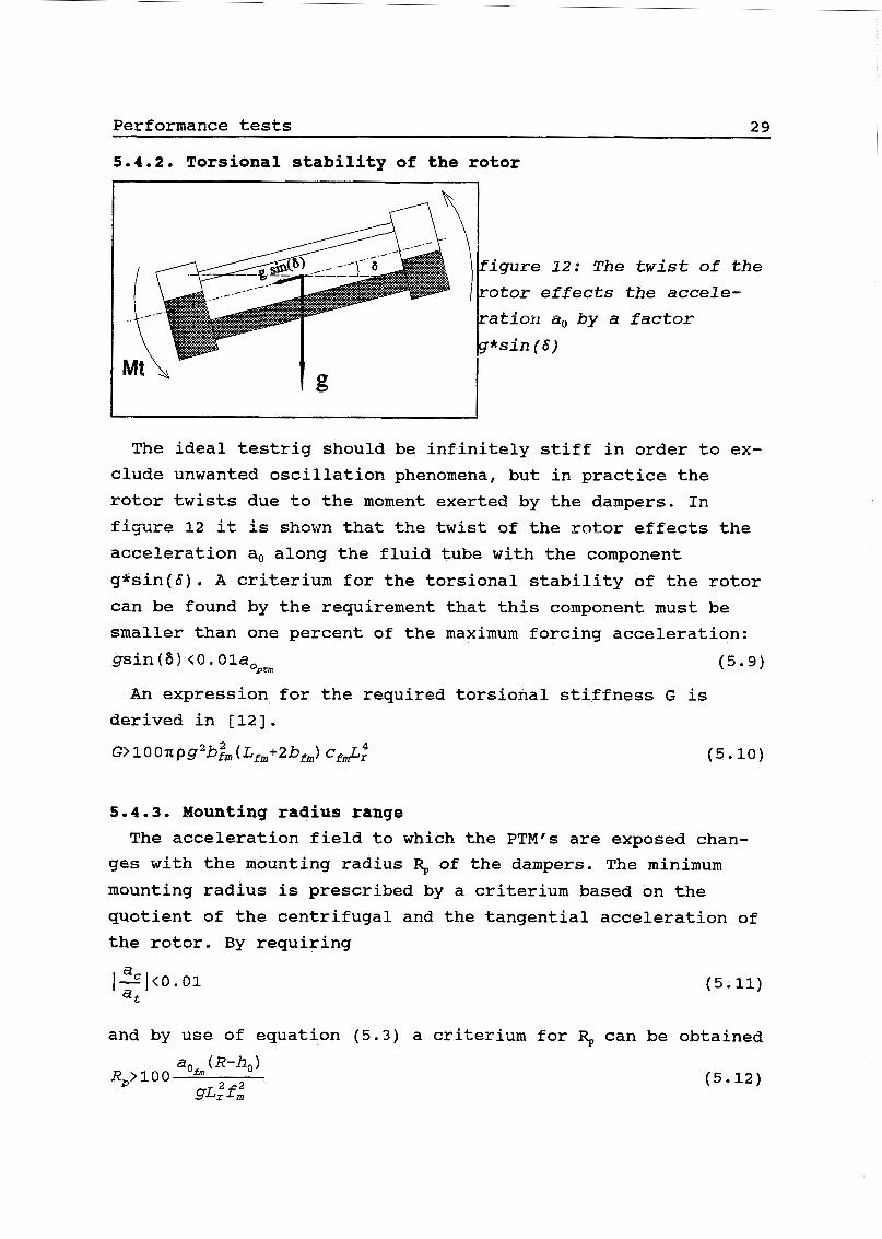
5.4.2. Torsional stability of the rotor

igure 12: The otor effects ation a, by a *s in (6)

twist of the the accele- factor

The ideal testrig should be infinitely stiff in order to ex- clude unwanted oscillation phenomena, but in practice the rotor twists due to the moment exerted by the dampers. In figUre 12 it is shown t h ~ t the +,vist ~f the rotor effects the acceleration a, along the fluid tube with the component g*sin(b). A criterium for the torsional stability of the rotor can be found by the requirement that this component must be smaller than one percent of the maximum forcing acceleration: gsin(6) <O. O1aogm ( 5 - 9 )

An expression for the required torsional stiffness G is derived in [12]. G>100xpg2b~,(Lf,+2bf,) cf&r (5.10)

5.4.3. Mounting radius range

ges with the mounting radius % of the dampers. The minimum mounting radius is prescribed by a criterium based on the quotient of the centrifugal and the tangential acceleration of the rotor. By requiring

The acceleration field to which the PTM's are exposed chan-

(5.11)

and by use of equation (5.3) a criterium for can be obtained

(5.12)


5.5. Testins a fliaht model When a flight model is tested on earth, the damper geometry

might need to be modified if the performance is calculated. Due to the rectangular shape of the gravitation field on earth, the fluid surface on earth differs from the one in ûïbit. The f l U i d surface in the endpots is now tilted, see figure 13. This will effect the tuning of the dampers and moreover the allowable fluid displacement in the endpots. The theoretical predictions must therefore be corrected for these geometry changes and the tests must be carefully defined to avoid fluid entering the vapour tubes.

i g u r e 13 : T i l t of the f l u i ä u r f a c e i n t h e e n d p o t s :

I I Mounted on the testing apparatus, the fluid surface in the

circular endpot becomes elliptically. For performance calculations this elliptical endpot surface must be translated into an effective circular endpot area with endpot radius beE. Also the allowable fluid displacement s and the distance ho between the centre of the fluid tube and the fluid surface are changed.

Computer implementation 31

6. computer imDlementation

6.1. Introduction At UCN two different programs, which calculate the damper-

performance, are available. One is made by Fokker and is written in the language Fortran. The other is made by UCN and is written in the language Pascal. In this report a description is given only of the Pascal program of UCN, which is moreover a software package. This package didn't give accurate results at first, so it was improved until the results were correct. With this software package calculation of the damper-

performance is possible, together with calculation of the fluid-displacement in the endpots, the fluid-velocity and the time-depenàent performance and fluid-displacement at simui- taneous excitations. Also calculation of a scaled test-model with its scaled behaviour is possible. In appendix A an example is given on how to design a damper

with this software.

6.2. Software Dackaqe 6.2.1. Units The improved software package is built around three units.

The first unit contains basic mathematic procedures and functions, the second unit takes care of the properties of the damper and the third unit contains the performance-specific procedures and functions.

6.2.2. Program Together with these three units there are at the moment two

programs. One to design the damper and the other to design the performance test model and to calculate the test apparatus performance criteria. These two programs use procedures which are listed in the units. The performance is calculated in two different manners. The

formula of ESA and the formula of Fokker are implemented. The performance is calculated as a function of the frequency-ratio


n/o,. Necessary for these calculations are three Bessel- functions J,, J2 and J,. These Besselfunctions are infinite series and can be represented by a sum. The sums which have to be used in these programs are derived in [12]. The fluid- displacement is calculated as a function of n/o, and the fluid- velocity is calculated as a function of the tube radius r. The

formulas which are used in this program to calctlate the velocity and the displacement are based on the Fokker elaboration. The simultaneous excitations performance is calculated as a function of time. The calculation of the performance test model is based on

the theory outlined in chapter 5. This program calculates the scale model geometry and the performance in test-conditions. It also calculates the requirements of the test-apparatus.

6.2.3. Input

files. One file contains the values of the geometry of the damper, the other file the values for the excitation that the damper experiences. Examples of these files are given in appendix B. The input of the PTM-program is separated in two files. One

file contains the flight model information. This is the same file which is used for the damper-design program. The other program contains the requirements which define the test series for the PTM. Examples of these files are given in appendix B.

The input of the damper-design program is separated in two

6.2.4. Output The output of all programs is written in columns of ascii-

text characters. These columns can be read by standard programs in order to draw diagrams of the performance, fluid- velocity etc.

Computer implementation 3 3

6.3. Software check In order to verify the correctness of the software it needs

to be checked. Five different checks were performed. - Check of the damperperformance accsrdimg to Fokker; - Check of the damperperformance according to ESA; - Check of simultaneous excitations; - Check of fluid-velocity; - Check of PTM calculation. The first issue of the Pascal program made by UCN, was

checked, modified and improved. After this improvement the results were equal with the results of the Fokker program. In order to verify whether the agreement of the two programs was not coincidental, the check was extended for different dampers ir! different circumstances. A11 the results showed satisfac- tory agreement. The fluid-displacement and the forcing acceleration were checked in the same manner. The calculation of the performance according to the ESA

elaborations was checked by comparison with the newest (improved) UCN program. Also this check was performed for different dampers and different circumstances. The check showed that the two methods calculate equal results for the performance. The calculation of simultaneous excitations was checked by

using equal frequencies for the different excitations. So it could be compared since the total amplitude of the different excitations was made equal to an amplitude at which the performance was calculated with the single excitation performance routine. The average performance calculated with simultaneous excitations must be equal to the performance calculated with single excitation. This check showed that the results were equal. The calculation of the fluid-velocity could not be verified

with another computer program, because such a program was not available. The velocity profiles were printed and similar profiles were found in literature [13] [14].


The check which was used for the program which calculates the PTM, was performed by setting the scale-factor to 1. The results from the PTM should be equal to the results calculated with the normal performance routine. This check was performed and the results agreed.

câlcUlâtes correct results for the different f~ncti~ns. All the results agreed within at least %O.

All these checks show that the Pascal program package

Conclusions and recommendations 35

7. Conclusion and recommendations The updated UCN program proved to be reliable. It calculates

the damper-performance correctly. With this program the next calculations can be performed. - Damper-performance as a function of the frequency ratio n/o,, - The forcing acceleration as a function of the frequency

- Fluid displacement as a function of the frequency ratio, - Fluid velocity as a function of the tube radius, - Damper-performance and fluid displacement as a function of

ratio in case of nutation (satellite dynamics),

time for simultaneous excitations. When the test results are compared with the theory, a

difference can be remarked. The theory predicts a constant performance as a function of the forcing acceleration, where the test results show an increasing or decreasing performance. The values of the test results for small forcing accelerations are equal to the predicted results.

accelerations it is recommended to regard the next points: - As an entrance effect only the effective tube length is

- At large nutation angles the flow becomes turbulent.

In order to predict the performance at large forcing

reckoned with.

Literature 36

8 . Literature Ancher, L.J.; Brink, H. v.d.; Pouw, A.: " S t u d y on p a s s i v e n u t a t i o n dampers volume I : l i t e r a t u r e s u r v e y and ana- l y s i s f ' December 1975 ESTEC contract Nr. 2318/74 AK

Ancher, L.J.; Brink, H. v.d.; Pouw, A.: " S t u d y on p a s s i v e n u t a t i o n dampers volume II: Damper selection and dimen- S i o n i n g f t December 1975 ESTEC contract Nr. 2318/74 AK

Ancher, L.J.; Brink, H. v.d.; Pouw, A.: " S t u d y on p a s s i v e n u t a t i o n dampers volume 111: Appendicesf1 December 1975 ESTEC contract Nr. 2318/74 AK

Werts, J . R . et al.: t t Spacecra f t a t t i t u d e d e t e r m i n a t i o n and controlff 3uly 1938

Crellin, E.B.: model o f the performance o f a f l u i d - i n - t u b e n u t a t i o n damper" November 1981 E.W.P. 1315 (Estec working paper no. 1315)

Crellin, E.B.: "Improved model o f the per formance o f a f l u i d - i n - t u b e n u t a t i o n damper" March 1982 E.W.P. 1329

(Estec working paper no. 1329)

Bongers, E. "In-orbit exper imen t s on COS-B n u t a t i o n damper per formance f f November 1984 TR-R-84-037

Kermans, S: "Des ign r e p o r t o f the CLUSTER p a s s i v e f l u i d - i n - t u b e dampers" March 1992 UCN document CL-UCN-RP-0024

Spiegel, M.R.:IITheory and problems o f F o u r i e r a n a l y s i s w i t h a p p l i c a t i o n s t o boundary v a l u e problemsf f 1974 Schaum's outline series USA

[lo] Batchelor, G.K. "An i n t r o d u c t i o n t o f l u i d dynamics" 1967

Cambridge university press USA

Literature 37

[li] Smallwood, J. ttDynamics r e p o r t f o r the c l u s t e r AOCMS SSDRtt January 1991, British Aerospace document, CL-BAe- RP-879

[12] Bakel, C . v.: t lNu ta t ion damping: d e r i v a t i o n s " 1993, UCN document, to be published

[13] Ancher, L.J. "Design and t e s t i n g o f a p a s s i v e n u t a t i o n damper f o r the s t a b i l i z a t i o n o f a s p i n n i n g s a t e l l i t e i n the l i m i t o f a very smal l n u t a t i o n angle" October 1974, International Astronautical Federation (IAF) XXV the congress

[14] Iguchi, M.; Park, Ge-M.; Akao, F.; Yamamoto, F. ItW s t u d y OR velocity p r o f i l e s of d e v e l o p i n g laminar oscil-latcry f l o w s i n a square duc t t t 1992, JSME series 11, vol. 35, no. 2 p. 158-164

Design example A . 1

Appendix A: Desiqn example

Introduction In this chapter an example is given of the complete damper design traject, including the design of the performance test model and the definition of the test plan. This exampbe is based on the design of the dampers for the Cluster-satellite. These dampers were designed to damp out the movements of the satellite caused by the antenna and nutation modes.

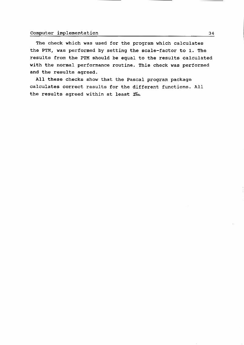
Performance reauirements The performance requirements define the minimal performance for a damper on a give frequency range and are drawn in figure A.1.

MA

EA

frequency- ratio

figure A.l: performance requirements

This figure shows that two dampers are needed to meet the requirements. Each damper takes care of one mode (EA or MA). Together they need to take care of the middle frequency range (N-mode) . An other particularly important requirement is that the mass of each damper shall be minimised. The dampers are tuned by adjustment of their endpot radius, so only the fluid tube radius and the fluid tube length are free to be chosen in the

Design example A. 2

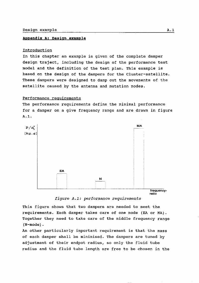
design process. The fluid tube radius influences the power- dissipation to the fourth power.

- -a4L a;

This equation shows that L should be maximised if possible, to obtain the highest P/aO. Besides, a long fluid tube will lead to a minimised nass ss well (see figure A.2)

CLUSTER Endpol r8dlUs and damper mass - b E A ...... _---- L U A ..........

6

4

9 - O 25

' E 2

1

O O 200 400 600 BOO 1000

L [mml

\

" '-..I- -- " '.

\

... .............. j . . . .I .................. '.._ I

........... i I

60

40

30

20

- E E - o

I ' o

f i g u r e A . 2 : The mass and endpot r a d i u s o f the tuned dampers v e r s u s the t u b e l e n g t h L.

Because the tube length L was limited up to 278 mm, this length was chosen for the dampers.

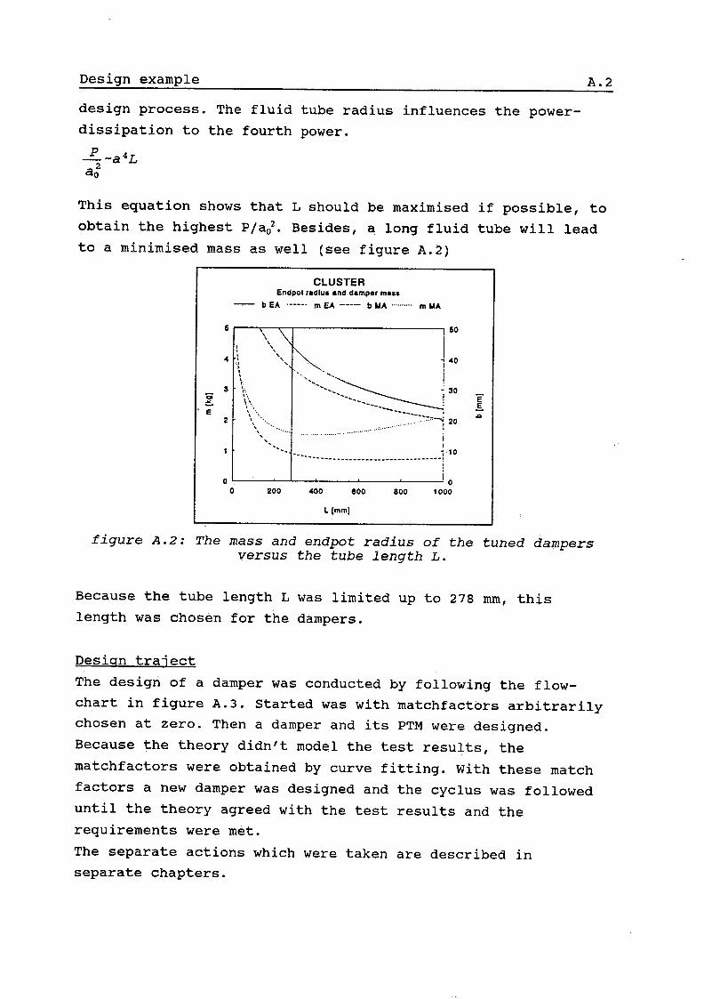
Desisn traject The design of a damper was conducted by following the flow- chart in figure A . 3 . Started was with matchfactors arbitrarily chosen at zero. Then a damper and its PTM were designed. Because the theory didn't model the test results, the matchfactors were obtained by curve fitting. With these match factors a new damper was designed and the cyclus was followed until the theory agreed with the test results and the requirements were met. The separate actions which were taken are described in separate chapters.


esign PTM

I curve f i t +, G factors

agrees w i t theory?

f i g u r e A . 3 : flow-chart d e s i g n traject

Damper desisn

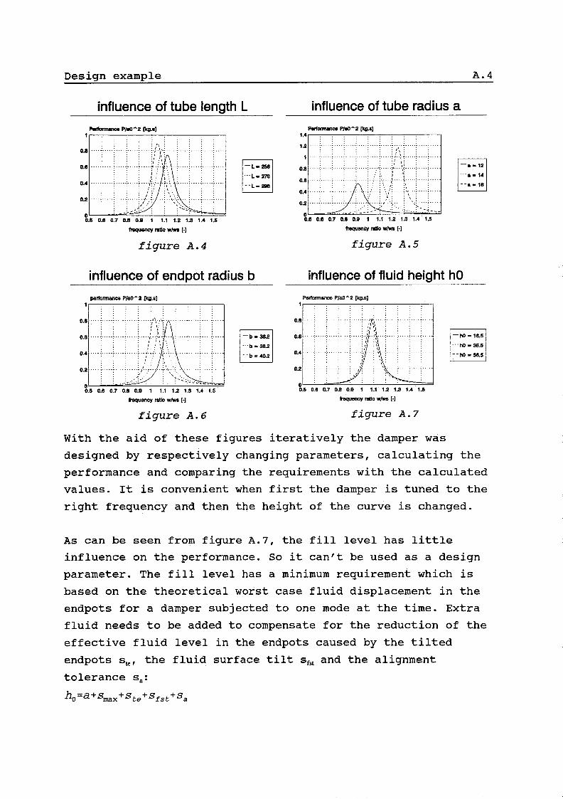
The dampers were designed by varying the design parameters until the performance was just a little above the required value. The required performance was given in a range of frequencies (see figure A . l ) . The damper was tuned at this range, which means that the peak of the performance curve is in this range. The performance will be above the required value when the performance at the two edges of the frequency range are above the required values. Now a damper was designed by "designing" the performance of the two edge-frequencies above the requirements. The influence of the design parameters on the performance is given in figures A . 4 to 8.7.


influence of tube length L influence of tube radius a

. . . .

Ob 0.6 0.7 0.6 O 9 1 1.1 1.2 13 1.4 15

f igure A . 4 f i g u r e A . 5

influence of endpot radius b influence of fluid height hO Pleo ̂ 2 rn.81

+equency ratio w k I-]

f i g u r e A.6 wnicv W h 1-1

f i g u r e A.7

With the aid of these figures iteratively the damper was designed by respectively changing parameters, calculating the performance and comparing the requirements with the calculated values. It is convenient when first the damper is tuned to the right frequency and then the height of the curve is changed.

As can be seen from figure A.7, the fill level has little influence on the performance. So it can't be used as a design parameter. The fill level has a minimum requirement which is based on the theoretical worst case fluid displacement in the endpots for a damper subjected to one mode at the time. Extra fluid needs to be added to compensate for the reduction of the effective fluid level in the endpots caused by the tilted endpots ster the fluid surface tilt sfst and the alignment tolerance sa:

-ho =a +smx +ste+ Sfs t+ sa

n

48.6 14.0 278. O 1.37 O O

LJ a I m I b cm1 ho Cml IJ I m l R [ m l Q!

B' :::O ~~ 38.2 36.5 278.0 1.37 O O

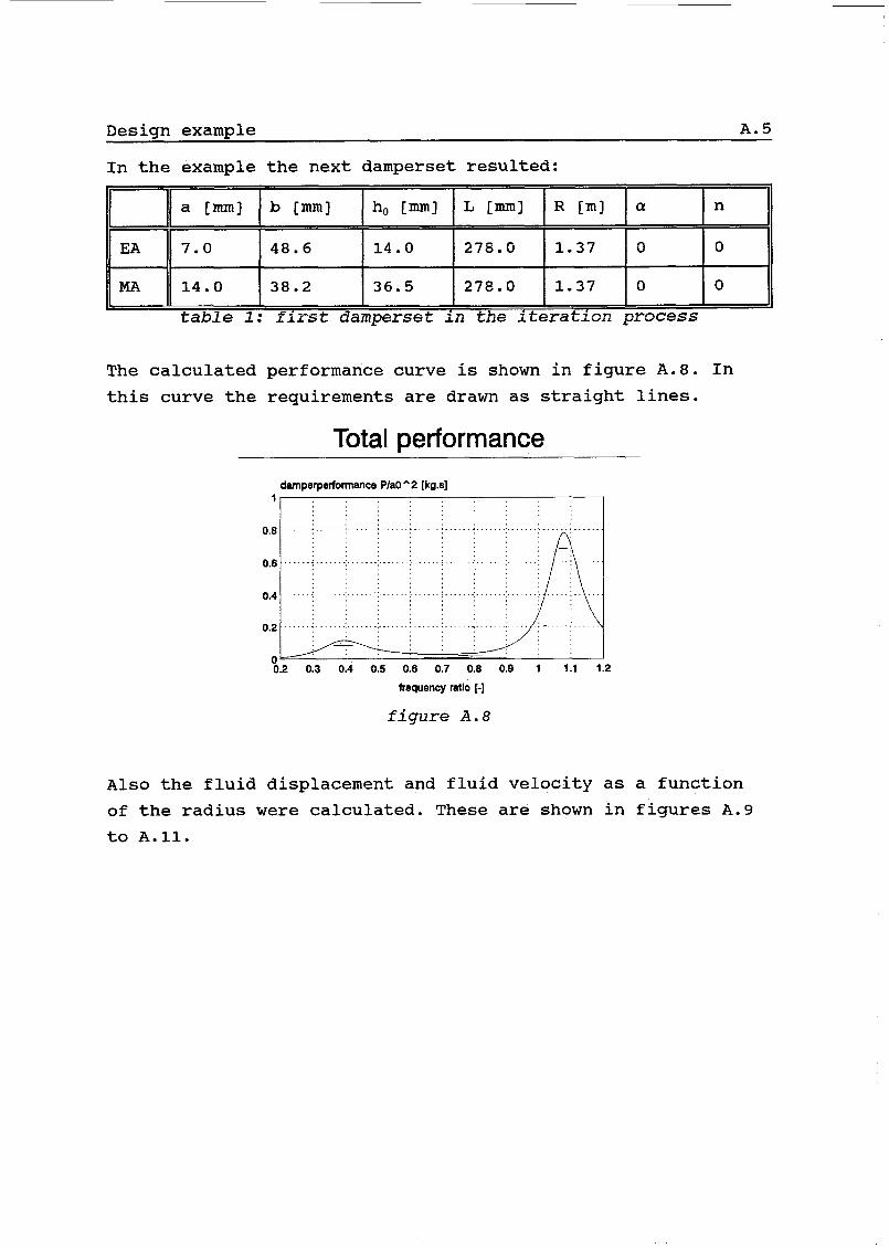
The calculated performance curve is shown in figure A . 8 . In this curve the requirements are drawn as straight lines.

Total performance damperperformance PlaO ^2 [kg.s]

.... . . . . :. ..... _ f ..... . . i ...... i . ...... i _ _ .......... .. i . . ..

u 0.2 0.3 0.4 0.5 0.6 0.7 0.8 0.9 i 1.1 1.2

frequency ratio [-I

f i g u r e A.8

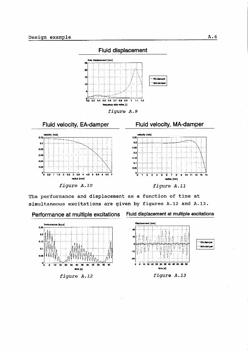
Also the fluid displacement and fluid velocity as a function of the radius were calculated. These are shown in figures A.9 to A.ll.

Design example A.6

FI u id d is DI ace ment

0.2 O 8 0.4 0.5 0.6 0.7 0.8 O S 1 1.1 1 2

fmvJmw ntlo W h [-I

figure A.9

Fluid velocity, EA-damper Fluid velocitv, MA-damper

. . . . . . . . . . . . . . . . . . . . . . . . . . . . . . . . . . . . . ' 0 0.5 1 1.5 2 25 9 3.5 4 4.5 5 5.5 8 6.5 7 - [mml

f i g u r e A . 1 O

* [Ml o s . . . . . . . . . . . . . . . . . . . . . . . . .

. . . . . . . . . . . . . . . . . . . .

. . . . . . . . . . .

O 1 2 S 4 5 6 7 8 S l O 1 1 1 2 1 3 1 4

radius [mm]

f i g u r e A.ll

The performance and displacement as a function of time at simultaneous excitations are given by figures A.12 and A.13.

Performance at multiple excitations Fluid displacement at multiple excitations

O 2 5

0 2 . . . . . . . . . . . . . . . .

,. ...... , ....... ..,. 0.15 . . . . .

0.1

0.06

O O 6 1 0 1 6 2 0 2 5 ~ 3 5 4 0 4 6 6 0 5 6 6 0

Gina IS1

f i g u r e A.12

- EA-dunper

f i g u r e A.13


PTM desisn

a [mml b [ml ho [ml

34.7 10.0 EA 5.0

As a result of the different environmental conditions in space and on earth, a scale model needs to be designed im order to be able to test the damper. The scale factor for the test model geometry needs to be defined and was calculated with:

L [ml

198.6

It is obvious that the damper couldn’t be tested at a l l the frequencies where it was calculated. So a selection of frequencies had to be made. Because the damper had to perform well at the required frequencies, it was convenient to chose frequencies in these ranges as testing frequencies. Most of the testing frequencies were situated around a peak in the performance curve. Because the testing apparatus exhibits internal friction, which causes extra damping, three dummy-runs had to be made. See chapter 5.2.

Desiqn example A. 8

50

o

Test results

- . . . . . . . . . . . . . . . . . . . . . . . . . . . . . . . . . . . . . . . . . . . . . . . . . . . . . . .

- PIH-rrirJde test resu 1 ts.

I I I I , I , , I I 1 t I I I # * I I , 1 1 1 1

The test-results showed a tendency which is illustrated in nigcire A.14.

Horizontally the amplitude of the damper displacement (which is a measurement for the forcing acceleration) is plotted and vertically the measured damper performance. Curve 1 was measured at a frequency ratio higher than that of the peak in the performance curve (see figure A.8). Curves 2, 4 and 7 were measured on top of the performance curve. Curve 8 and 9 were measured at a lower frequency ratio. When the damper results are compared with the calculated results, they need to be scaled back. Now a surface plot can be made of the performance dependent on two parameters, being the forcing acceleration and the frequency ratio. Such a plot is given in figure A.15. In this plot only the MA-mode is drawn.

Design example A. 9

f igure A.25: Testresults o f the performance as a function o f forcing acceleration and frequency r a t i o

Match factors

After testing the performance proved to be different from the calculated performance, so the two new rnatch-factors had to be calculated. Then the whole design traject was conducted again. This was done in the same manner as the first design sequence. Thus a set of two match-factors was chosen, the new performance was calculated and the results were compared with the test-results. This sequence was repeated until the damper just met the requirements.

Final desicrn

After repeating the design traject, the final design of the flight model was determined at:

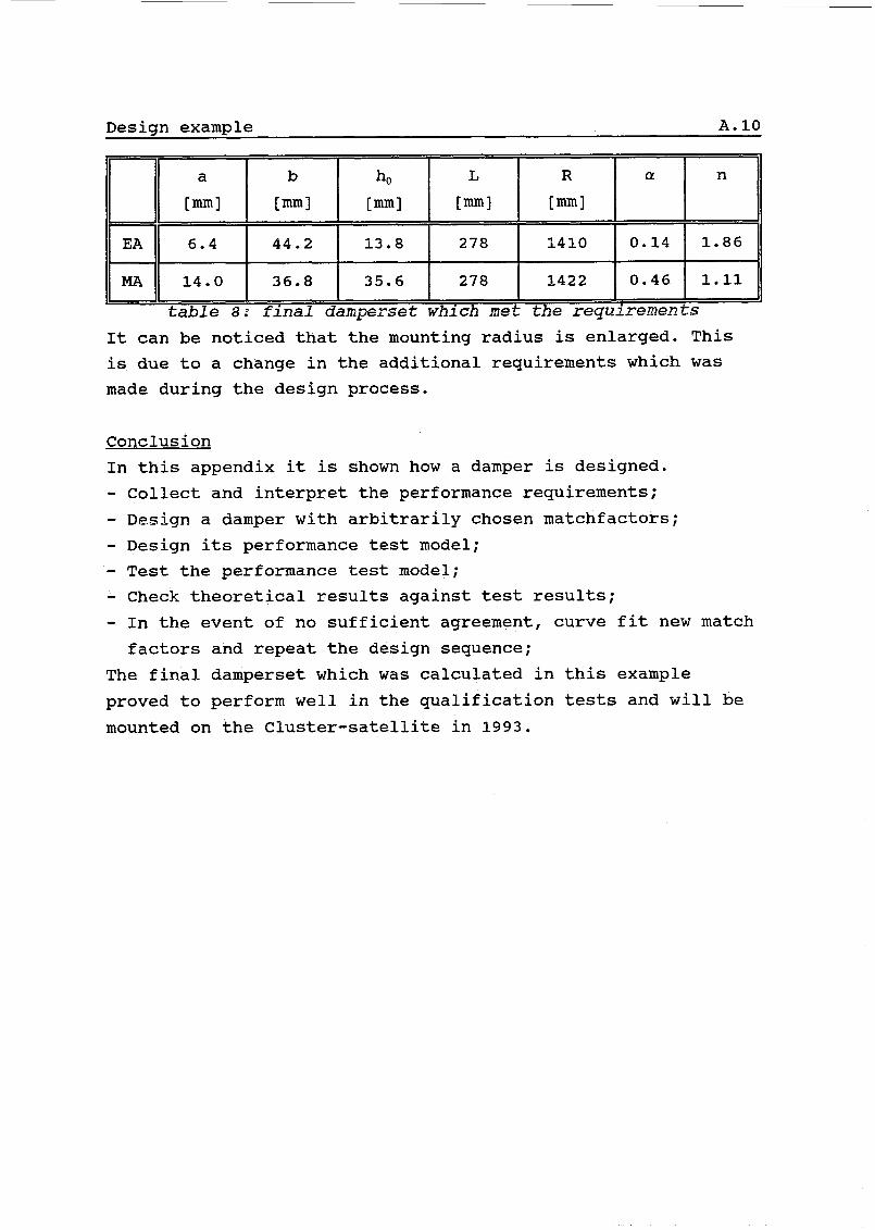
b h0 L R Q

[ml [ml [ml [ml

44.2 13.8 278 1410 0.14

:::o 36.8 35.6 278 1422 0.46

n, r-I

Conclusion In this appendix it is shown how a damper is designed. - Collect and interpret the performance requirements; - Design a damper with arbitrarily chosen matchfactors; - Design its performance test model; - Test the performance test model; - Check theoretical results against test results; - In the event of no sufficient agreement, curve fit new match factors and repeat the design sequence;

The final damperset which was calculated in this example proved to perform well in the qualification tests and will be mounted on the Cluster-satellite in 1993.

n

1.86

1.11

Pascal-inputfiles B.l

Appendix B: Pascal inputfiles

Damper inputfile

EA - dampe r equator i a 1

û.ûu aifa 0.00 nn

7.00e-3 a

48.6e-3 b

14.Oe-3 hO 278.0e-3 L

1370.0e-3 R

0.5 z 15 sr 3 f lu id

MA- damper

equator i a 1 0.00 a l f a

0.00 nn

14.00e-3 a

38.2e-3 b 36.5e-3 hO

278.Oe-3 L

1370.0e-3 R 0.5 z 15 sr 3 f lu id

Performance requirements inputfile

0.311

1.120

29

1 .O8

1 O0

28

0.01 0472

1000

4

0.422 6.43e-3

0.898 7.42e-2

1.024 2.42e-2

1.087 8.76e-3

fn-start

f n-end

N g o i n t s

f v

R g o i n t s T-test I temperature of t e s t

Theta , i n i t i a l nutat ion angle

N-transient I curve g r i d of t rans ient graph

N-f req

fn[1] aOt11, frequency i? amplitude o f

fn[2] a0121, simultaneous exc i ta t ions

fnC33 aOC31,

fnC41 aOt41 I

I P/aOA2 p l o t x-axis: fn-start t o fn-end

curve g r i d of P/aOA2 graph

I frequency r a t i o o f f lu id ve loc i t y calc.

, curve g r i d of v e l o c i t y graph

I nmkr o f simultaneous exc i ta t ions

!!!!!!Filenames and dampertype i n damperprogram!!!!!!!

Pascal-inputfiles B.2

PTM requirements inputfile

EA- damper

O . 00500

2.00

190 9.81 20

5

3

1 .o 1.1

O. O 1 0472

O

0.5

1 .o

a , tube radius o f PTM

Ra

IP 9 , g r a v i t y

T-test , temperature of tes t

Ngo in ts , Nunber o f t e s t s

Noa , Number o f modes

fn-start, To ta l frequency range from

fn-end , fn-star t t o fn-end

theta , i n i t i a l nu ta t i on angle

2.8e-5 6.43e-3 , freq, aOmin, a0max

1.97e-4 1.17e-1 , frequencies a t whic.. the new accelerat ion

1.8e-4

, mounting rad ius on ro to r , moment o f i n e r t i a o f ro to r

2.42e-2 , requirements s t a r t and the acc. requirements

MA-damper

o. 01000

2.00

190

9.81

20

5

3

1 .o 1 .I

O. O1 0472

O

0.5

1 .o

a , tube radius o f PTM

Ra

IP , moment o f i n e r t i a of ro to r

9 , g r a v i t y

T-test , temperature o f t es t

Ngo in ts , Number o f t e s t s

Noa , Nunber o f modes

fn-start, Tota l frequency range from

fn-end , fn-star t t o fn-end theta , i n i t i a l nu ta t i on angle

2.8e-5 6.43e-3 , freq, aOmin, a0max

1.97e-4 1.17e-1 , frequencies a t which the new accelerat ion

1.8e-4 2.42e-2 , requirements s t a r t and the acc. requirements

, mounting rad ius on r o t o r

nutation damping theory and computer implementation - tu/e

Documents