numerical treatment of two-phase flow in · pdf filenumerical treatment of two-phase flow in...

INTERNATIONAL JOURNAL OF c© 2012 Institute for ScientificNUMERICAL ANALYSIS AND MODELING Computing and InformationVolume 9, Number 3, Pages 505–528

NUMERICAL TREATMENT OF TWO-PHASE FLOW IN

CAPILLARY HETEROGENEOUS POROUS MEDIA BY

FINITE-VOLUME APPROXIMATIONS

HELMER ANDRE FRIIS AND STEINAR EVJE

This paper is dedicated to the memory of Professor Magne S. Espedal (1942-2010)

Abstract. This paper examines two-phase flow in porous media with heterogeneous capillarypressure functions. This problem has received very little attention in the literature, and constitutesa challenge for numerical discretization, since saturation discontinuities arise at the interfacebetween the different homogeneous regions in the domain. As a motivation we first consider aone-dimensional model problem, for which a semi-analytical solution is known, and examine somedifferent finite-volume approximations. A standard scheme based on harmonic averaging of theabsolute permeability, and which possesses the important property of being pressure continuousat the discrete level, is found to converge and gives the best numerical results. In order toinvestigate two-dimensional flow phenomena by a robust and accurate numerical scheme, a recentmulti point flux approximation scheme, which is also pressure continuous at the discrete level, isthen extended to account for two-phase flow, and is used to discretize the two-phase flow pressureequation in a fractional flow formulation well suited for capillary heterogenity. The correspondingsaturation equation is discretized by a second-order central upwind scheme. Some numericalexamples are presented in order to illustrate the significance of capillary pressure heterogeneity intwo-dimensional two-phase flow, using both structured quadrilateral and unstructured triangulargrids.

Key words. two-phase flow, heterogeneous media, capillary pressure, finite volume, MPFA,unstructured grids

1. Introduction

The study of two-phase flow in porous media has significant applications in areassuch as hydrology and petroleum reservoir engineering. The flow pattern is mainlygoverned by the geometric distribution of absolute permeability, which may beanisotropic and highly heterogeneous, the form of the relative permeability andcapillary pressure functions and gravity [4]. The corresponding system of partialdifferential equations describing the flow consists of an elliptic and an essentiallyhyperbolic part, usually denoted the pressure- and saturation equation, respectively.This system is rather challenging, and quite a lot of research has been devoted toits solution during the last decades.

In recent years several discretization methods that can treat unstructured gridsin combination with discontinuous and anisotropic permeability fields have beendeveloped for the elliptic pressure equation. Important examples are the flux-continuous finite volume schemes introduced in e.g. [11, 12, 25, 13, 15, 5, 6], whichhave been termed multi point flux approximation methods (MPFA) schemes, andthe mixed finite element (MFE) and related schemes, e.g., [1, 2, 9, 20, 18]. The MFEand related methods solve for both control-volume pressure and cell face velocitiesleading to a globally coupled indefinite linear system (saddle point problem), whilethe more efficient MPFA methods only solve for control-volume pressure and have

Received by the editors February 7, 2011 and, in revised form, May 1, 2011.2000 Mathematics Subject Classification. 65M60, 76S05, 35R05.

505

506 H.A. FRIIS AND S. EVJE

a locally coupled algebraic system for the fluxes that yield a consistent continuousapproximation, while only requiring one third the number of degrees of freedomof the mixed method when compared on a structured grid (and a quarter in threedimensions). The latter methods are clearly advantageous, particularly for time-dependent problems, as the extra degrees of freedom required by the mixed methodadd further computational complexity and a severe penalty to simulation costs. Forthe saturation equation some higher order schemes have been employed, as well asvarious types of so called fast tracking schemes, but the standard first order upwindscheme is still widely used in commercial simulators.

However, the main body of research literature devoted to two-phase flow inporous media concerns flow in the absence of capillary pressure, or assumes a ho-mogeneous capillary pressure function in the domain. Obviously, there are a numberof flow cases for which these assumptions are valid, but this observation is neverthe-less noticeable since heterogeneity in capillary pressure may often have a significanteffect on the flow pattern, and in certain cases it can be as important as absolutepermeability heterogeneity [19].

From the very sparse literature devoted to capillary pressure heterogeneity inporous media, we would like to mention the work of Yortsos and Chang [27]. Theystudied analytically the capillary effect in steady-state flow in one-dimensional (1D)porous media. They assumed a sharp, but continuous transition of permeabilityto connect different permeable media of constant permeabilities. The paper byvan Duijn and de Neef [26] on the other hand, provided a semi-analytical solu-tion for time-dependent countercurrent flow in 1D heterogeneous media with onediscontinuity in permeability and capillary pressure. Niessner et al. [24] discussthe performance of some fully implicit vertex-centered finite volume schemes, whenimplementing the appropriate interface condition for capillary heterogeneous me-dia. The recent paper by Hoteit and Firoozabadi [19] presents an MFE method fordiscretising the pressure equation together with a discontinuous Galerkin methodfor the saturation equation. They introduced a new fractional flow formulationfor two-phase flow, which is suited for applying MFE in media with heterogeneouscapillary pressure. Some numerical examples are presented, including a comparisonwith the 1D semi-analytical solution from [26], demonstrating good performance ofthe numerical scheme.

The simulation of two-phase flow in porous media with capillary pressure het-erogeneity represents a challenge for the actual numerical discretization. This isparticularly due to the fact that saturation discontinuities arise at the interface be-tween the different homogeneous regions of the domain, as a result of the require-ment of capillary pressure continuity. Moreover, since these are rather involvednonlinear problems, very few analytical results are known, making it more difficultto gain confidence in the results produced by the numerical schemes. Clearly, asdiscussed in [26], the capillary pressure may also actually become discontinuous atthe interface in some situations. This depends on the form of the capillary pres-sure curve (the entry pressure) together with the actual type of two-phase flow inthe problem. In the more usual situations where a wetting phase is displacing anon-wetting phase, this phenomenon will not occur. Moreover, since this partic-ular situation does not introduce any new fundamental issues with respect to thenumerical treatment of these problems, we only consider examples with capillarypressure continuity at the interface in this paper.

As noted in [19] MPFA methods have not yet been demonstrated to be of valuefor heterogeneous media with contrast in capillary pressure functions. This fact

NUMERICAL MODELING OF TWO-PHASE FLOW 507

is a prime motivation for the present paper. We examine a standard scheme in1D based on harmonic averaging of the absolute permeability as well as a moredirect “naive” type of discretization and present detailed comparisons with thesemi-analytical solutions from [26]. The scheme based on harmonic averaging ofthe absolute permeability, which can be considered as a ”1D MPFA scheme”, isfound to converge and gives the best numerical results.

The ”1D MPFA scheme” moreover, naturally provides a discrete approximationwith a built-in pressure continuity. From the numerical results obtained in the1D model problem, this property is considered to be important for the numericaltreatment of these problems. Only recently, some multidimensional MPFA schemeswith this property have been developed and tested for one-phase elliptic problems[13, 14, 16]. In this paper we extend the schemes from [13] and [16], which aredeveloped for cell-centered quadrilateral and triangular grids, respectively, to two-phase flow problems, and also present some numerical examples. We use the recentfractional flow formulation from [19], and moreover, solve the saturation equationby using the second-order central upwind scheme from [23].

The paper is organised as follows. Section 2 gives a description of the two-phaseflow model, whereas Section 3 discusses two different implicit pressure explicit sat-uration (IMPES) formulations suitable for the numerical solution of this model.In Section 4 we study a 1D model problem using some different discretizations,and compare with semi-analytical solutions. Section 5 describes a recent discretepressure continuous 2D MPFA scheme and its extension to two-phase flow. Fur-thermore, Section 6 briefly describes the central-upwind scheme used in the dis-cretization of the saturation equation. Some numerical examples are presentedin Section 7, that illustrate two-phase flow behavior with and without capillarypressure heterogeneity. Finally, conclusions follow in Section 8.

2. The two-phase flow model

In this section we present the governing equations for immiscible two-phase flowin a domain Ω of a porous medium. The mass balance equation for each of the fluidphases reads

(1) φ∂(ρisi)

∂t+∇ · (ρi~ui) = ρiqi, i = w, o,

where φ is the porosity of the medium, i = w indicates the wetting phase (e.g.water) and i = o indicates the nonwetting phase (e.g. oil). Moreover, ρi, si, ~ui andqi are, respectively, the density, saturation, velocity and external flow rate of thei-phase. The phase velocity is given by Darcy’s law

(2) ~ui = −kriµi

K∇(pi − ρigZ), i = w, o,

where K is the absolute permeability tensor of the porous medium, g is the gravita-tional constant and Z is the depth, i.e. the negative of the actual z-coordinate whenthe z-axis is in the vertical upward direction. pi, µi and kri are, respectively thepressure, viscosity and relative permeability of the i-phase. Moreover, the capillarypressure is given by

(3) Pc(~x, sw) = po − pw,

where ~x denotes the spatial coordinate vector, and the saturation constraint reads


(4) sw + so = 1.

It is useful to introduce the phase mobility functions

λi(~x, si) =kriµi

, i = w, o,

the total mobility

λ(~x, s) = λw + λo,

and the total velocity

~u = ~uw + ~uo,

where s = sw. Finally, the so called fractional flow functions fi are defined as

fi(~x, s) =λi

λ, i = w, o.

Usual boundary conditions for this model are the no-flow boundary conditions

(5) ~ui · ~n = 0, i = w, o,

where ~n is the outer unit normal to the boundary δΩ of Ω. Alternatively, the flowrate(s) or oil pressure and water saturation may be prescribed at various parts ofδΩ.

3. IMPES formulations

We now reformulate the equations of Section 2 such that they become applica-ble for the IMPES formulation. Assuming the the fluids are incompressible, theequations (1) and (4) give rise to the following equation for the total velocity ~u

(6) ∇ · ~u = qw + qo ≡ q.

Using (6) together with equations (3) and (2) we obtain an elliptic equation for thepressure p = po, which reads

(7) −∇ · (λK∇p) = −∇ · (λwK∇Pc + (λwρw + λoρo)g∇Z) + q,

where the corresponding total velocity is given as

(8) ~u = −K(λ∇p− λw∇Pc − (λwρw + λoρo)g∇Z).

Again using the assumption of incompressibility, an evolution equation for thesaturation s = sw is obtained from equations (1) and (2) which reads

(9) φ∂s

∂t+∇ · (Kfw(s)λo(∇Pc + (ρw − ρo)g∇Z) + fw(s)~u) = qw.

Observe that Pc 6= 0 gives us a convection-diffusion equation for the saturation s.The IMPES solution strategy now goes as follows. For a given initial saturation

s(~x) = s0(~x), we solve the pressure equation (7), and then solve the saturationequation (9) based on the computed velocity field to update the saturation s. Inthe classical IMPES method the pressure and saturation fields are updated with thesame frequency. However, since the saturation field usually changes more rapidlyin time than the pressure field, it is natural to employ smaller time steps whensolving the saturation equation.


In the improved IMPES method proposed by Chen et al. [10] the pressureequation is updated with a (possibly) variable time-step ∆tp, whereas the smallervariable inner time-steps ∆ts, used for the saturation equation, is determined bythe relation

(10) ∆ts =DSmax

(∂s∂t )max

,

where (∂s∂t )max denotes the maximum value of ∂s∂t in the grid, and DSmax is the

maximum variation of the saturation to allow. The latter quantity obviously needsto be specified from the outside. Note that the time-step determined by (10) ob-viously also must obey the CFL condition required by the underlying numericalscheme for the saturation equation.

By using this approach Chen et al. [10] obtained a considerable improvementof the classical IMPES method, and were i.a. able to solve a benchmark coningproblem, previously unattainable for the classical IMPES formulation, 6.7 timesfaster than a comparative sequential solution method. We remark that Chen et al.[10] did not study problems including capillary pressure effects, which may seriouslylimit the usefulness of the IMPES formulation, due to the strict CFL conditionsenforced by the usual explicit methods, e.g., Runge-Kutta methods, employed forthe time-discretization of the saturation equation.

However, in this paper we are interested in a somewhat different fractional flowformulation, recently introduced by [19], which is also applicable for the IMPESsolution strategy. In order to simplify the notation we first define the potentials

(11) Ψi = pi − ρigZ, i = w, o,

and also the capillary pressure potential

(12) Ψc = Pc − (ρo − ρw)gZ.

The idea in the new fractional flow formulation ([19]) is to introduce the velocities

(13) ~ua = −λK∇Ψw,

and

(14) ~uc = −λoK∇Ψc.

It is now easily established that

~u = ~ua + ~uc,

and, moreover, that~uw = fw(s)~ua.

Equipped with this information, the pressure- and saturation equations in this newfractional flow formulation, may be expressed as

(15) −∇ · (λK∇Ψw) = ∇ · (λoK∇Ψc) + q,

and

(16) φ∂s

∂t+∇ · (fw(s)~ua) = qw.

where the potential Ψw and the water saturation s are the unknown variables, andthe velocity ~ua is given in equation (13). It should be noted that equation (16), incontrast to equation (9), is a pure convective equation. The capillary pressure effectsare then exclusively connected to the pressure equation (15) in this formulation anddoes not at first sight influence the CFL condition in equation (16). However, thevelocity ~ua (produced from the pressure equation) is obviously a major contributor


−2 −1.5 −1 −0.5 0 0.5 1 1.5 20

0.1

0.2

0.3

0.4

0.5

0.6

0.7

0.8

0.9

1

X

Sw

Saturation

harmonicarithmeticanalytic

−2 −1.5 −1 −0.5 0 0.5 1 1.5 20

0.1

0.2

0.3

0.4

0.5

0.6

0.7

0.8

0.9

1

X

Sw

Saturation


−2 −1.5 −1 −0.5 0 0.5 1 1.5 20

0.1

0.2

0.3

0.4

0.5

0.6

0.7

0.8

0.9

1

X

Sw

Saturation


−2 −1.5 −1 −0.5 0 0.5 1 1.5 20

0.1

0.2

0.3

0.4

0.5

0.6

0.7

0.8

0.9

1

X

Sw

Saturation

harmonicanalytic

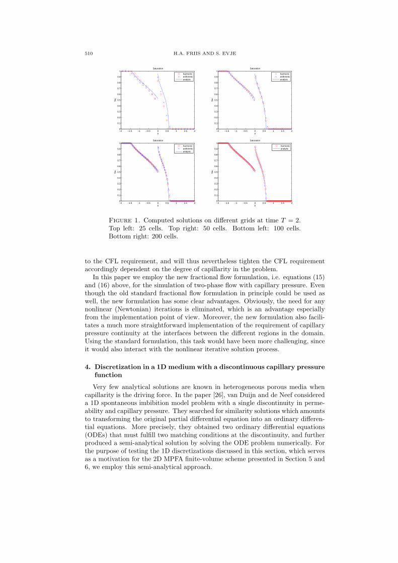
Figure 1. Computed solutions on different grids at time T = 2.Top left: 25 cells. Top right: 50 cells. Bottom left: 100 cells.Bottom right: 200 cells.

to the CFL requirement, and will thus nevertheless tighten the CFL requirementaccordingly dependent on the degree of capillarity in the problem.

In this paper we employ the new fractional flow formulation, i.e. equations (15)and (16) above, for the simulation of two-phase flow with capillary pressure. Eventhough the old standard fractional flow formulation in principle could be used aswell, the new formulation has some clear advantages. Obviously, the need for anynonlinear (Newtonian) iterations is eliminated, which is an advantage especiallyfrom the implementation point of view. Moreover, the new formulation also facili-tates a much more straightforward implementation of the requirement of capillarypressure continuity at the interfaces between the different regions in the domain.Using the standard formulation, this task would have been more challenging, sinceit would also interact with the nonlinear iterative solution process.

4. Discretization in a 1D medium with a discontinuous capillary pressure

function

Very few analytical solutions are known in heterogeneous porous media whencapillarity is the driving force. In the paper [26], van Duijn and de Neef considereda 1D spontaneous imbibition model problem with a single discontinuity in perme-ability and capillary pressure. They searched for similarity solutions which amountsto transforming the original partial differential equation into an ordinary differen-tial equations. More precisely, they obtained two ordinary differential equations(ODEs) that must fulfill two matching conditions at the discontinuity, and furtherproduced a semi-analytical solution by solving the ODE problem numerically. Forthe purpose of testing the 1D discretizations discussed in this section, which servesas a motivation for the 2D MPFA finite-volume scheme presented in Section 5 and6, we employ this semi-analytical approach.


The model problem we are interested in takes the form of a nonlinear diffusionequation given by

(17)∂s

∂t+

∂

∂x

(

k(x)fw(s)λo(s)∂Pc(x, s)

∂x

)

= 0, x ∈ [−L,L].

This equation is obtained from (9) by neglecting the gravity, setting total velocityand source term equal to zero, as well as assuming constant porosity φ to be 1 forthe sake of simplicity only. Initial data s0(x) = s(x, t = 0) is given as

(18) s0(x) =

1, x < 0;0, x > 0.

Furthermore, the permeability k(x) is given by

(19) k(x) =

kl, x < 0;kr, x > 0.

and fw(s) is the water fractional flow function fw(s) =λw(s)

λw(s)+λo(s)with the mobil-

ities λw and λo defined as λi =kri(s)µi

for i = w, o. Moreover, the capillary pressure

function Pc is given by

(20) Pc(x, s) =1

√

k(x)J(s),

where J(s) is the Leverett function. Here we have implicitly set porosity φ andinterfacial tension σ to be 1, for simplicity reasons only. In the following we alsoassume that the viscosity is characterized by M = µo

µw= 1. We consider the van

Genuchten model, see [26] and references therein, where relative permeability andcapillary pressure are given by

J(s) = (s−1/m − 1)1−m

krw(s) = s1/2(1− [1− s1/m]m)2(21)

kro(s) = (1 − s)1/2(1 − s1/m)2m,

where 0 < m < 1 is a constant to be specified. In the numerical experiments carriedout below we have used the following values

(22) kl = 4.2025, kr = 0.5625, m =2

3.

Following the procedure outlined in [26] we solve for the similarity solution whichwe shall refer to as the analytical solution. This solution is used to evaluate thenumerical approximation.

We consider a simple finite volume discretization for the numerical solution ofthe initial-value problem (17) and (18) with data as specified above. We discretizethe spatial domain Ω = [−L,L] into N non-overlapping gridblocks Ωi:

[−L,L] := Ω = ∪Ni=1Ωi, Ωi = [xi−1/2, xi+1/2], ∆xi = xi+1/2 − xi−1/2.

We assume, for simplicity, a regular grid with ∆xi = ∆x. Similarly, we considera constant time step size ∆t. Given the water saturation sn ≈ s(x, tn) at time tn,we must solve for the updated saturation sn+1 at time tn+1. For that purpose weconsider the discrete scheme

(23)sn+1i − sni

∆t+D−

(

ki+1/2[fwλo]ni+1/2D+P

nc,i

)

= 0, i = 1, . . . , N,


Harmonic Arithmetic∆x ‖E(s)‖1 q ‖E(s)‖1 q0.1600 0.1463 - 0.1351 -0.0800 0.0332 - 0.0595 -0.0400 0.0236 0.49 0.0390 0.610.0200 0.0178 0.41 0.0243 0.680.0100 0.0106 0.75 0.0133 0.87

Table 1. Estimated L1-error, ‖E(s)‖1 = ∆x∑

i |si−sref(xi)|, andconvergence order, q, where sref is the reference solution obtainedby solving the ODE system resulting from (17)–(19) and si refersto the numerical solution based on (23).

where D+ and D− are the discrete differential operators applied on a sequence aiand defined by

D+ai =ai+1 − ai

∆x, D−ai =

ai − ai−1

∆x.

Note that we have used a simple forward Euler discretization in time (explicitscheme). Consequently, we must also choose the time step according to the CFLcondition

∆t

∆x2max(

√

kl,√

kr)maxi

[fw(si)λo(si)J′(si)] ≤

1

2.

The average [fwλo]i+1/2 is obtained by taking an arithmetic average. For the av-erage ki+1/2 of the permeability function at the cell interface i+ 1/2 we check two

different approaches: (i) arithmetic average kA; (ii) harmonic average kH .

(24) kAi+1/2 =ki + ki+1

2, kHi+1/2 =

2kiki+1

ki + ki+1.

We have computed solutions at time T = 2 on three different grids corresponding toN = 25 cells, N = 50 cells, and N = 75 cells on a domain corresponding to L = 2.We refer to Fig. 1 for the results. The comparison between using kA and kH revealsthat the harmonic averaging tends to give approximate solutions that lie closer tothe analytical solution. Finally, we have also computed the solution on a finer gridof N = 200 cells by using the scheme with harmonic averaged permeability kH

demonstrating (virtually) convergence to the analytical solution. We refer also toTable 1 for estimates of the error measured in L1-norm as the grid is refined. Itseems that the rate of convergence is approaching 1. This relatively low rate ofconvergence is expected and must be understood in light of the severe discontinuitypresent in the solution.

It is well known (see e.g. [12]) that MPFA schemes in fact are generalizations ofthe scheme with harmonic averaging of the absolute permeability in higher spatialdimensions. Thus it is clear that the scheme which employs kH automatically fulfillsthe requirement of continuity in capillary pressure at x = 0. However, for the sakeof completeness of the paper, we present the arguments for this fact. For simplicity,we first consider the standard prototype pressure equation

(25)d

dx(k

dp

dx) = 0,

where p is the pressure. We are now interested in the discrete flux approximationproduced by the one-dimensional MPFA scheme at xi+1/2. The MPFA approach


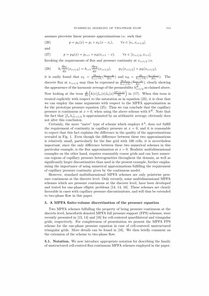
assumes piecewise linear pressure approximations i.e. such that

(26) p = pL(x) = pi + aL(x− xi), ∀x ∈ [xi, xi+1/2],

and

(27) p = pR(x) = pi+1 + aR(xi+1 − x), ∀x ∈ [xi+1/2, xi+1].

Invoking the requirements of flux and pressure continuity at xi+1/2 i.e.

(28) kidpLdx

(xi+1/2) = ki+1dpRdx

(xi+1/2), pL(xi+1/2) = pR(xi+1/2),

it is easily found that aL = 2ki+1

ki+1+ki(pi+1−pi

∆xi) and aR = 2ki

ki+1+ki(pi−pi+1

∆xi). The

discrete flux at xi+1/2 may thus be expressed as 2kiki+1

ki+1+ki(pi+1−pi

∆xi), clearly showing

the appearence of the harmonic average of the permeability kHi+1/2 as claimed above.

Now looking at the term ∂∂x

(

k(x)fw(s)λo(s)∂Pc(x,s)

∂x

)

in (17). When this term is

treated explicitly with respect to the saturation as in equation (23), it is clear thatwe can employ the same arguments with respect to the MPFA approximation asfor the prototype pressure equation (25). Thus we can conclude that the capillarypressure is continuous at x = 0, when using the above scheme with kH . Note thatthe fact that [fwλo]i+1/2 is approximated by an arithmetic average, obviously doesnot alter this conclusion.

Certainly, the more “naive” type of scheme which employs kA, does not fulfillthe requirement of continuity in capillary pressure at x = 0, and it is reasonableto expect that this fact explains the difference in the quality of the approximationsrevealed in Fig. 1. Even though the difference between these two approximationsis relatively small, particularly for the fine grid with 100 cells, it is neverthelessimportant, since the only difference between these two numerical schemes in thisparticular example, is the flux approximation at x = 0. Realistic multidimensionalexamples on the other hand, requires reasonably coarse grids and can have numer-ous regions of capillary pressure heterogeneities throughout the domain, as well assignificantly larger discontinuities than used in the present example, further empha-sizing the importance of using numerical approximations fulfilling the requirementof capillary pressure continuity given by the continuous model.

However, standard multidimensional MPFA schemes are only pointwise pres-sure continuous at the discrete level. Only recently, some multidimensional MPFAschemes which are pressure continuous at the discrete level, have been developedand tested for one-phase elliptic problems [13, 14, 16]. These schemes are clearlyfavorable in cases with capillary pressure discontinuitues, and will thus be extendedto two-phase flow in this paper.

5. A MPFA finite-volume discretization of the pressure equation

Two MPFA schemes fulfulling the property of being pressure continuous at thediscrete level, henceforth denoted MPFA full pressure support (FPS) schemes, wererecently presented in [13, 14] and [16] for cell-centered quardilateral and triangulargrids, respectively. For completeness of presentation we present the MPFA FPSscheme for the one-phase pressure equation in case of cell-centered unstructuredtriangular grids. More details can be found in [16]. We then briefly comment onthe extension of the scheme to two-phase flow.

5.1. Notation. We now introduce appropriate notation for describing the familyof unstructured cell-centred flux-continuous MPFA schemes employed in the paper.


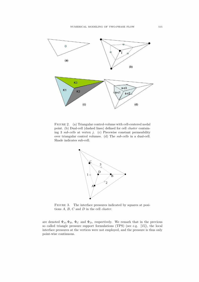
5.1.1. Grid Cell. The grid (i.e. the collection of control-volumes or cells) isdefined by the triangulation of the vertices (or corner points) j. Each grid cell isassigned a grid point (nodal point) xi, which here is equal to the cell centroid (seeFigure 2(a)). In the cell-centered formulation presented here flow variables androck properties are distributed to the grid cells and are therefore control-volumedistributed (CVD). The value of the numerical solution in the cell is denoted byΦi = φi(xi). Two adjacent grid cells are termed neighbours if they share the samecell interface or cell edge. The permeability (conductivity) tensor K is assumed tobe piecewise constant, with respect to cell values (see Figure 2(c)). The control-volume is denoted Ωi for i = 1, ..., NE, where NE is the number of control-volumes(or cells) in the grid, and its corresponding boundary is δΩi.

5.1.2. Cluster. In the cell centered formulation continuous flux and pressure con-straints are imposed locally with respect to each cluster cj of cells that are attachedto a common grid vertex j. The degree of the cluster cj is defined as the number

of cell interfaces that meet at the vertex and is denoted by N jd . For each interior

vertex the number of cells in the cluster is also equal to N jd . An example of a cell

cluster with three cells and corresponding dual grid cell is shown in Figure 2(b).

5.1.3. Dual-Cell. For each cell cluster cj , a dual-cell is defined as follows: Foreach cell edge attached to the vertex of the cluster, connect the edge mid-pointek to the grid points (i.e. cell centres) of the two neighboring cells within thecluster that share the common edge (one cell centre if the edge is a boundary). Itis not generally necessary to choose ek as the mid-point, but in this paper otherpossibilities are not considered. The dual-cell will then be defined by the resultingpolygon comprised of the contour segments connecting the N j

d cell mid-points asindicated by the dashed lines in Figure 2(b).

5.1.4. Sub-Cell. Subcells result when the dual-cells overlay the primal triangulargrid. Each triangle (control-volume) is then comprised of three quadrilateral sub-cells. Each sub-cell is defined by the anti-clockwise loop joining the parent trianglecell-centre, triangle right-edge mid-point, central cluster vertex, triangle left-edgemid-point and back to the triangle centre as illustrated in Figure 2(d). The volume

of the dual-cell is seen to be comprised of N jd sub-cells, where each sub-cell of a

parent triangle is attached to the same distinct vertex and thus cluster cj .

5.1.5. Sub-Interface. The edge point ek divides a cell interface into two seg-ments, the term sub-interface will be used to distinguish each of the two segmentsfrom the total cell interface.

5.1.6. Local Interface Pressures. In the MPFA methods, the following twocontinuity conditions should be fulfilled for every sub-interface: flux continuity andpressure continuity. One of the main advantages of the this type of formulation isthat it involves only a single degree of freedom per control-volume, in this case theprimal grid cell pressure Φi, while maintaining continuity in pressure and normalflux across the control-volume faces. This is achieved by introducing local interfacepressures that are expressed in terms of the global pressure field via local algebraicflux continuity conditions imposed across control-volume faces. In the MPFA FPSscheme full pressure continuity along each sub-interface in the grid is ensured byintroducing an auxiliary interface pressure at the common grid vertex of the clusteras well as on each sub-interface (at point ek) belonging to the dual-cell, thus yielding

N jd+1 interface pressures per dual-cell. Referring to Figure 3, the interface pressures


Figure 2. (a) Triangular control-volume with cell-centered nodalpoint. (b) Dual-cell (dashed lines) defined for cell cluster contain-ing 3 sub-cells at vertex j. (c) Piecewise constant permeabilityover triangular control volumes. (d) The sub-cells in a dual-cell.Shade indicates sub-cell.

1

2

3

A

B

C

D

Figure 3. The interface pressures indicated by squares at posi-tions A, B, C and D in the cell cluster.

are denoted ΦA,ΦB, ΦC and ΦD, respectively. We remark that in the previousso called triangle pressure support formulations (TPS) (see e.g. [15]), the localinterface pressures at the vertices were not employed, and the pressure is thus onlypoint-wise continuous.


1

2

3

A

B

C

D

1

2

3

A

B

C

D

q

q

q

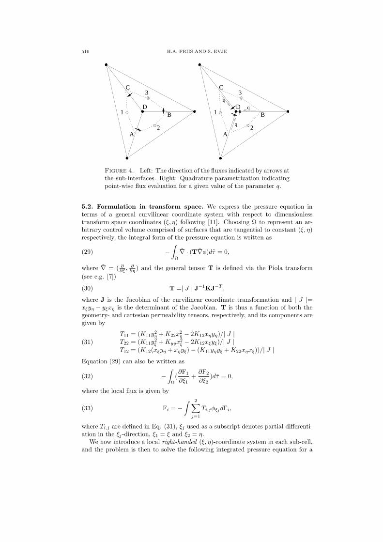
Figure 4. Left: The direction of the fluxes indicated by arrows atthe sub-interfaces. Right: Quadrature parametrization indicatingpoint-wise flux evaluation for a given value of the parameter q.

5.2. Formulation in transform space. We express the pressure equation interms of a general curvilinear coordinate system with respect to dimensionlesstransform space coordinates (ξ, η) following [11]. Choosing Ω to represent an ar-bitrary control volume comprised of surfaces that are tangential to constant (ξ, η)respectively, the integral form of the pressure equation is written as

(29) −∫

Ω

∇ · (T∇φ)dτ = 0,

where ∇ = ( ∂∂ξ ,

∂∂η ) and the general tensor T is defined via the Piola transform

(see e.g. [7])

(30) T =| J | J−1KJ−T ,

where J is the Jacobian of the curvilinear coordinate transformation and | J |=xξyη − yξxη is the determinant of the Jacobian. T is thus a function of both thegeometry- and cartesian permeability tensors, respectively, and its components aregiven by

T11 = (K11y2η +K22x

2η − 2K12xηyη)/| J |

T22 = (K11y2ξ +Kyyx

2ξ − 2K12xξyξ)/| J |

T12 = (K12(xξyη + xηyξ)− (K11yηyξ +K22xηxξ))/| J |(31)

Equation (29) can also be written as

(32) −∫

Ω

(∂F1

∂ξ1+

∂F2

∂ξ2)dτ = 0,

where the local flux is given by

(33) Fi = −∫ 2

∑

j=1

Ti,jφξjdΓi,

where Ti,j are defined in Eq. (31), ξj used as a subscript denotes partial differenti-ation in the ξj-direction, ξ1 = ξ and ξ2 = η.

We now introduce a local right-handed (ξ, η)-coordinate system in each sub-cell,and the problem is then to solve the following integrated pressure equation for a


triangular grid

(34) −3

∑

s=1

(

∫

δΩsi

(T s∇φ) · ~nstdΓ) = 0,

where the superscript s is connected to a given (quadrilateral) sub-cell within the

triangle (see Figure 2(d)), ~nst is the transform space sub-cell normal vector and δΩs

i

denotes the outer boundary of the sub-cell in transform space.In general the sub-cell tensor can be defined via the isoparametric mapping

(35) ~r = (1− ξ)(1 − η)~r1 + ξ(1 − η)~r2 + ξη~r3 + (1− ξ)η~r4

where ~r = (x, y), ~ri, i = 1, ...4 are the subcell corner position vectors and 0 ≤ ξ, η ≤1, with ~r1 and ~r3 corresponding to the cell-centre and dual-cell centre respectivelyand ~r2 and ~r4 correspond to the mid-points of the triangle edges connected to thedual-cell centre. As a result each quadrilateral subcell is transformed into a unitquadrant in transform space. The tensor is then approximated in a local coordinatesystem aligned with the two faces of the dual-cell connected to the given sub-cell.

5.3. The MPFA FPS approximation. Assuming a bi-linear approximationwithin each sub-cell (Figure 3), the pressures in the three sub-cells may be writtenin the local (ξ, η)-coordinate-system as

(36) φ1 = Φ1 + (ΦA − Φ1)ξ + (ΦC − Φ1)η + (ΦD +Φ1 − ΦA − ΦC)ξη,

(37) φ2 = Φ2 + (ΦB − Φ2)ξ + (ΦA − Φ2)η + (ΦD +Φ2 − ΦB − ΦA)ξη,

and

(38) φ3 = Φ3 + (ΦC − Φ3)ξ + (ΦB − Φ3)η + (ΦD +Φ3 − ΦC − ΦB)ξη.

Physical space flux continuity conditions are defined with respect to each cellcluster. We define the fluxes in a counter-clock wise manner with respect to thesub-interfaces of each cluster. Now let D denote the cluster vertex in the illustrativecluster shown in Figure 4(left). We let FA be the flux out of cell 1 through thesub-interface at AD, FB be the flux out of cell 2 through the sub-interface at BDand FC be the flux out of cell 3 through the sub interface at CD (see Figure 4(left)).

Introducing a quadrature parametrization q such that 0 ≤ q ≤ 1 (see Fig-ure 4(right)), the point-wise flux continuity is accommodated along each of thelines AD, BD and CD, respectively.

Utilizing equation (33), the three flux continuity equations then read

FAD = −(T11|1AD(q)(ΦA − Φ1) + (ηT11)|1AD(q)(ΦD +Φ1 − ΦA − ΦC)

+ T12|1AD(q)(ΦC − Φ1) + T12|1AD(q)(ΦD +Φ1 − ΦA − ΦC))

= T12|2AD(q)(ΦB − Φ2) + T12|2AD(q)(ΦD +Φ2 − ΦB − ΦA)

+ T22|2AD(q)(ΦA − Φ2) + (ξT22)|2AD(q)(ΦD +Φ2 − ΦB − ΦA),

(39)

FBD = −(T11|2BD(q)(ΦB − Φ2) + (ηT11)2BD(q)(ΦD + Φ2 − ΦB − ΦA)

+ T12|2BD(q)(ΦA − Φ2) + T12|2BD(q)(ΦD +Φ2 − ΦB − ΦA))

= T12|3BD(q)(ΦC − Φ3) + T12|3BD(q)(ΦD +Φ3 − ΦC − ΦB)

+ T22|3BD(q)(ΦB − Φ3) + (ξT22)3BD(q)(ΦD +Φ3 − ΦC − ΦB),

(40)


and

FCD = −(T11|3CD(q)(ΦC − Φ3) + (ηT11)3CD(q)(ΦD +Φ3 − ΦC − ΦB)

+ T12|3CD(q)(ΦB − Φ3) + T12|3CD(q)(ΦD +Φ3 − ΦC − ΦB))

= T12|1CD(q)(ΦA − Φ1) + T12|1CD(q)(ΦD +Φ1 − ΦA − ΦC)

+ T22|1CD(q)(ΦC − Φ1) + (ξT22)1CD(q)(ΦD +Φ1 − ΦA − ΦC).

(41)

Note that the notation AD(q) etc. serves to indicate the dependence of theflux continuity point on the quadrature parametrization. Note that AD(0) = A

and AD(1) = D, while 0 < q < 1 extracts points ~P along the line AD such that~P = ~A+ q( ~D − ~A) (and of course analogously along the lines BD and CD).

However, in order to close the above equation system (39), (40) and (41) anadditional equation is needed. For that purpose we utilize the integral form of thepartial differential equation over an auxillary dual-cell (see Figure 5(left)) i.e.

(42) −∮

δΩdjAUX

(T∇φ) · ~ntdΓ = 0,

where ΩdjAUX

denotes the (transform space) auxillary dual-cell connected to a vertexwith index j. The actual size of the auxillary dual cell control-volume is a furtherdegree of freedom to be chosen within the scheme, and is parameterized by thevariable c where 0 ≤ c ≤ 1. Note that for c = 0 we obtain the usual dual-cell, whilethe auxillary control-volume tends to zero as c → 1. Yet another free parameter isneeded to specify this scheme. We let p be the quadrature parametrization neededfor the point-wise flux evaluation needed at the sub-interfaces in the auxillary dual-cell in equation (42). p should be chosen such that c ≤ p < 1. Discretisizingequation (42) following the above sub-cell approach, we then obtain a dual-cellequation which reads

T11|1C1(c,p)(ΦA − Φ1) + (ηT11)1C1(c,p)(ΦD +Φ1 − ΦA − ΦC)

+ T12|1C1(c,p)(ΦC − Φ1) + (ξT12)1C1(c,p)(ΦD +Φ1 − ΦA − ΦC)

+ T12|11A(c,p)(ΦA − Φ1) + (ηT12)11A(c,p)(ΦD +Φ1 − ΦA − ΦC)

+ T22|11A(c,p)(ΦC − Φ1) + (ξT22)11A(c,p)(ΦD +Φ1 − ΦA − ΦC)

+ T11|2A2(c,p)(ΦB − Φ2) + (ηT11)2A2(c,p)(ΦD +Φ2 − ΦB − ΦA)

+ T12|2A2(c,p)(ΦA − Φ2) + (ξT12)2A2(c,p)(ΦD +Φ2 − ΦB − ΦA)

+ T12|22B(c,p)(ΦB − Φ2) + (ηT12)22B(c,p)(ΦD +Φ2 − ΦB − ΦA)

+ T22|22B(c,p)(ΦA − Φ2) + (ξT22)22B(c,p)(ΦD +Φ2 − ΦB − ΦA)

+ T11|3B3(c,p)(ΦC − Φ3) + (ηT11)3B3(c,p)(ΦD +Φ3 − ΦC − ΦB)

+ T12|3B3(c,p)(ΦB − Φ3) + (ξT12)3B3(c,p)(ΦD +Φ3 − ΦC − ΦB)

+ T12|33C(c,p)(ΦC − Φ3) + (ηT12)33C(c,p)(ΦD +Φ3 − ΦC − ΦB)

+ T22|33C(c,p)(ΦB − Φ3) + (ξT22)33C(c,p)(ΦD +Φ3 − ΦC − ΦB)

= 0,

(43)

where the notation C1(c, p), 1A(c, p) etc serves to indicate the dependence of theparameters c and p on the position of the discrete flux evaluation on the half edges inthe auxillary dual cell, which are parallel with the lines C1, 1A (see Figure 5(right))etc. in transform space. Note that C1(0, 0) = C, 1A(0, 0) = 1 (where 1 in this lastequation obviously means the triangle centroid of cell 1 in Figure 5(right)).

The equations (39), (40), (41) and (43) now define a linear system of equations interms of dual-interface pressures and the primal cell-centered pressures for all cellsconnected to the cluster vertex. This system may generally be written as follows

(44) MfΦf = McΦc,


1

2

3

A

B

C

D

c

1

2

3

A

B

C

pppD

Figure 5. Left: Example range of auxillary control volumes(dashed) centered around the vertex D and depending on the pa-rameter c. Right: Fluxes out of auxillary dual cell and quadratureparametrization indicating point-wise flux evaluation for a givenvalue of the parameter p at the sub-interfaces in the auxillary dual-cell.

where Mf and Mc are matrices. In this particular case of a three cell clusterΦf = (ΦA,ΦB,ΦC ,ΦD)T and Φc = (Φ1,Φ2,Φ3)

T . Obviously this may be doneanalogously for an arbitrary cell cluster. Thus the interface pressures can be ex-pressed in terms of the primal cell-centered pressures via equation (44), which isperformed in a preprocessing step thus eliminating them from the discrete system.

5.4. Flux and finite volume approximation. Utilizing the above local alge-braic flux contiuity conditions, the discrete flux F across a cell sub-interface in thegrid may be written as a linear combination of grid cell centre values Φi in the dualgrid:

F = −∑

i∈NjF

tiΦi,(45)

where N jF is the index set of grid points involved in the flux approximation and

N jF contains a maximum of N j

d cells. The coefficients ti resemble conductancesand are called the transmissibilities associated with the flux interface. Since theflux must be zero when Φi is constant for all i ∈ N j

F , all consistent discretizationsmust satisfy the condition

∑

i∈Nj

Fti = 0. The net flux across each cell-interface

(triangle-edge) is comprised of two sub-interface fluxes, calculated by assemblingcontributions from the two dual grid cells corresponding to the two triangle-edgevertices.

Finally the discrete divergence over the primal triangle cells is then comprised ofassembled fluxes that are algebraically linear functions of the primal cell-centeredpressures. This defines the so called MPFA FPS scheme recently presented in [16],for elliptic problems.

5.5. Extensions to account for two-phase flow. Untill now we have presentedthe discretization methodology for the one-phase flow pressure equation. However,


the extension needed to treat the present two-phase flow flux term i.e.

−∮

δΩi

(λ(s)K∇Ψw) · ~ndS

is indeed very limited. Let λv represent the total mobility at the vertex v in the grid,which can be found by the interpolation procedure i.e. equation (56), described inSection 6 below. Since the mobility λ is a scalar quantity, a two-phase flow sub-interface flux Ftf can then be written as

(46) Ftf = λvF,

where F is the flux given in equation (45), which obviously is supposed to belongto the cluster with vertex v. Alternatively, from an implemenation point of view,it is sufficient to multiply the transmissibilities in equation (45) with λv.

5.6. Approximating the capillary pressure flux. The capillary pressure flux,which is a right hand side contribution in the integrated form of the pressure equa-tion, reads

∮

δΩi

(λoK∇Ψc) · ~ndS.

It can be approximated by the MPFA FPS scheme as follows. Assume that asaturation field is given in the control-volume cell centers such that we know thecell centered capillary pressures, and consider the scheme described in Section 5.3(except that the transmissibilites must be multiplied with λov, where v again is anindex identifying the vertex). Due to the construction of the MPFA FPS algorithmthe capillary pressure field will be continuous (which is physically correct) and thecapillary pressure flux over a given sub-interface Ftcp simply reads

(47) Ftcp = λovF,

where the flux F (given in equation (45)) now can be computed explicitly fromknown cell-centered capillary pressure potentials Ψc.

Remark 1. As noted in the introdution, there are in fact cases i.a. depending onthe entry pressure and the type of flow, where the capillary pressure may be dis-continuous at interfaces between different rock types (even if continuity in capillarypressure is the usual situation). See [26] for a more detailed discussion. In suchcases the MPFA FPS scheme will have to be modified, by introducing a double setof auxillary pressures in the formulation. Additional equations will then be neededto close the local equation system. Such equations may be found from knowledgeof the saturation values in some parts of the domain. However, we emphasize thatthis situation can not occur in the cases considered in this paper where water isdisplacing oil, and, moreover, do not introduce any new fundamental issues withrespect to the numerical treatment of these problems,

5.7. Computing the velocity ~va. When Ψw is found by solving the pressureequation (15) using the MPFA FPS scheme, the velocity ~va = −λK∇Ψw, or moreprecisely the flux of ~va over a given interface in the grid, must be computed in orderto be used as input in the saturation equation (16). This can be done by computingeach of the sub-interface fluxes, which in this case can be computed explicitly fromequation (46).


jv

j1

j3

j2

v

v

vM

M

j1

j3

Mj2

nj1

j2

j3

n

n

Figure 6. Notation in a triangular grid.

6. Discretization of the saturation equation

The relatively recent so called central-upwind schemes for hyperbolic conser-vation laws were introduced in [22]. These schemes extend the central schemesdeveloped by Kurganov and Tadmor in [21], and in fact coincide for a scalar PDEsuch as the saturation equation. The central-upwind schemes belong to the class ofGodunov-type central schemes, and their construction is based on the exact evolu-tion of picewise polynomial reconstructions of the approximate solution, achievedby integrating over Riemann fans. Their resolution is comparable to the upwindschemes, but in contrast to the latter, they do not employ Riemann solvers andcharacterisitic decomposition, which makes them both simple and efficient for avariety of multidimensional PDE systems.

For the case of unstructured triangular grids a (second-order) central-upwindscheme was recently presented in [23]. In this paper we employ the scheme from[23] for the spatial semi-discretization of the saturation equation. In the followingwe present some details pertaining to this discretization.

Consider as an example the scalar conservation law

(48)∂s

∂t+

∂f(s)

∂x+

∂g(s)

∂y= 0.

In order to introduce some necessary notation, let us denote the control volumesin the triangulation by Vj , with corresponding areas ∆Vj . For a given index j, theneighbouring control volumes of Vj are termed Vjk, k = 1, 2, 3. Moreover, the jointedge between Vj and Vjk is denoted by Ejk and is assumed to be of length hjk.Finally, the outward unit normal to Vj on the kth edge is njk, and the midpoint ofEjk is Mjk (see Figure 6).

Now let

(49) snj ≈ 1

∆Vj

∫

vj

s(~x, tn)dV

be the cell average on all the cells Vj, which are assumed to be known at the timetn, and let

(50) sn(x, y) =∑

j

snj (x, y)χj(x, y)

be a reconstructed piecewise polynomial, where χj(x, y) is the characteristic func-tion of the control volume Vj , s

nj (x, y) is a two-dimensional polynomial yet to be


determined and, finally, snjk(x, y) denotes the corresponding polynomial that is re-constructed in the control volume Vjk.

Discontinuities in the interpolant sj along the edges of Vj (where we for simplicityomit time dependence n and spatial dependence (x, y)) propagate with a maximalinward velocity and a maximal outward velocity ainjk and aoutjk , respectively. Forconvex fluxes in the scalar case these fluxes can be estimated as

ainjk(Mjk) = −min∇F (sj(Mjk)) · njk,∇F (sjk(Mjk)) · njk, 0,

aoutjk (Mjk) = max∇F (sj(Mjk)) · njk,∇F (sjk(Mjk)) · njk, 0,where F = (f, g).

Now the algorithmic development of the central-upwind scheme goes as follows.The above local speeds of propagation are used to determine evolution points thatare away from the propagating discontinuities. An exact evolution of the recon-struction at these evolution points is followed by an intermediate piecewise poly-nomial reconstruction and finally projected back onto the original control volumes,providing the cell averages at the next time step sn+1

j .A semi-discrete scheme is then obtained at the limit

(51)d

dtsn = lim

∆t→0

sn+1 − sn

∆t.

Fortunately most of the terms on the right-hand side of (51) vanish in the limit as∆t → 0, leaving only the integrals of the flux functions over the edges of the cells,which must be determined by an appropriate quadrature. We follow [23] and use asimple midpoint quadrature, which leads to the following semi-discrete scheme

(52)d

dtsn = − 1

∆Vj

3∑

k=1

hjk

ainjk + aoutjk

[(ainjkFoutjk +aoutjk F in

jk ) ·njk −ainjkaoutjk (soutjk − sinjk)],

where we have employed the notation soutjk = sjk(Mjk), sinjk = sj(Mjk), F injk =

F (sinjk) and F outjk = F (soutjk ). We refer to [23] for more details about this scheme,

which can be applied to systems of conservation laws in an analogous manner.The particular second-order reconstruction used in this paper is taken from [8].

The first step is to compute a least-squares estimate of the gradient of a scalarfield f on the triangle Vj , which is denoted by ∇jf . ∇jf is computed by followingthe algorithm reported in [3]. The gradient Djf are then limited component bycomponent as

(53) Djf = MM(∇jf, ∇j1f, ∇j2f, ∇j3f),

where ∇jkf is the least-squares gradient estimate on Vjk and MM is the commonmultivariable MinMod limiter function defined by

(54) MinMod(x1, x2, . . .) :=

minjxj if xj > 0 ∀j,maxjxj if xj < 0 ∀j,0 otherwise.

Furthermore, the gradients Djf is used to construct a piecewise linear reconstruc-tion for the point values of each triangle edge Ejk as follows

(55) uj(~x) = uj +MM(Dju · (~x− ~xj),Djku · (~x− ~xj)),

where Djku is the limited gradient estimate on Vjk , ~xj is the center of Vj and~x ∈ Ejk. As noted in [8], this double use of the MinMod limiter minimizes spuriousoscillations while preserving the second-order accuracy of the reconstruction.


Figure 7. Left: The domain in example 1. The middle layer isleast permeable. Right: The domain in example 2. The circularinclusion is least permeable.

Figure 8. The unstructured triangulation used in example 2.

6.1. Interpolation of the mobility. In Sections 5.5 and 5.6 an interpolation ofthe mobility (λ or λ0, respectively) from the cell-centered values is needed at thevertices in the grid. This is done by the following formula

(56) λv =

∑

i:Vi∈Vvi(λi∆Vi)

∑

i:Vi∈Vvi(∆Vi)

,

where λv is the mobility at the vertex v and Vvi denotes the set of triangles neigh-bouring this same vertex.

7. Computational examples

In the following we present two examples demonstrating effects of capillary pres-sure heterogeneity in two-phase flow using a structured cartesian grid and an un-structured triangulation, respectively. Here we consider a capillary pressure func-tion of the form

(57) Pc(s) = − φ√kln(s),


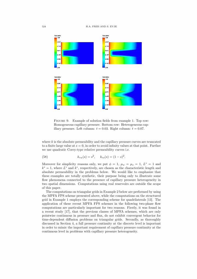
Figure 9. Example of solution fields from example 1. Top row:Homogeneous capillary pressure. Bottom row: Heterogeneous cap-illary pressure. Left column: t = 0.03. Right column: t = 0.07.

where k is the absolute permeability and the capillary pressure curves are truncatedto a finite large value at s = 0, in order to avoid infinity values at that point. Furtherwe use quadratic Corey-type relative permeability curves i.e.

(58) krw(s) = s2, kro(s) = (1− s)2.

Moreover for simplicity reasons only, we put φ = 1, µw = µo = 1, L∗ = 1 andk∗ = 1, where L∗ and k∗, respectively, are chosen as the characteristic length andabsolute permeability in the problems below. We would like to emphasize thatthese examples are totally synthetic, their purpose being only to illustrate someflow phenomena connected to the presence of capillary pressure heterogeneity intwo spatial dimensions. Computations using real reservoirs are outside the scopeof this paper.

The computations on triangular grids in Example 2 below are performed by usingthe MPFA FPS scheme presented above, while the computations on the structuredgrid in Example 1 employs the corresponding scheme for quadrilaterals [13]. Theapplication of these recent MPFA FPS schemes in the following two-phase flowcomputations are particularly important for two reasons. Firstly, it was found ina recent study [17], that the previous classes of MPFA schemes, which are onlypointwise continuous in pressure and flux, do not exhibit convergent behavior fortime-dependent diffusion problems on triangular grids. Secondly, as thoroughlydiscussed in Section 4, a full pressure continuity at the discrete level is importantin order to mimic the important requirement of capillary pressure continuity at thecontinuous level in problems with capillary pressure heterogeneity.


Figure 10. Example of solution fields from example 2. Toprow: Homogeneous capillary pressure. Bottom row: Heterogeneouscapillary pressure. Left column: t = 1.0. Right column: t = 2.0.

7.1. Example 1. We consider displacement of oil by water in the 0.5× 13 layered

rectangular domain, initially filled with oil, which is shown in Figure 7 (left). Theisotropic permeability is equal to 0.01 in the middle layer and 1 otherwise. Water isinjected uniformly through the left vertical boundary, and the boundary conditionsare as follows. The two horizontal boundaries are closed, and the oil pressuredifference between the right and left vertical boundaries is put to 1. Moreover, weimpose a saturation equal to 1 at the left vertical boundary, whereas the saturationis put to 0 at the right vertical boundary.

Numerical computations (with a 50 × 75 structured rectangular grid) are per-formed using both a capillary homogeneous (k is put to 1 in equation (57)) andcapillary heterogeneous domain. Results are presented in Figure 9 for two differ-ent simulation times. The flow behavior with homogeneous capillary pressure is asexpected essentially governed by the permeability field such that the displacementprocess is very much delayed in the middle low permeability layer, and, moreoverexhibits a smooth behavior typical of standard diffusion problems.

The simulation results in the case of capillary pressure heterogeneity on the otherhand, demonstrates a substantially more complex flow behavior. In particular,we observe saturation discontinuites that have arosen at the two boundaries ofthe middle low permeability layer. Furthermore, it is clearly seen that water haspenetrated the low permeable domain to a much wider extent than in the case withhomogeneous capillary pressure.

7.2. Example 2. The 2× 2 quadratic domain with a circular inclusion as well asthe unstructured grid with 3738 triangles is shown in Figure 7 (right) and Figure 8,respectively. The isotropic permeability is equal to 0.01 in the circular inclusion and


1 otherwise. The four boundaries are closed in this example. Water is injected atthe lower left corner in the domain (source strength equal to 1), which is otherwisefilled with oil. A corresponding sink (with source strength equal to −1) is placedat the upper right corner.

Numerical computations (with the triangulation shown in 7 (right)) are againperformed using both a capillary homogeneous (k is put to 1 in equation (57)) andcapillary heterogeneous domain. Results are presented in Figure 10 for two differentsimulation times.

Again we observe the significant difference in flow behavior between the twocases. The case with homogeneous capillary pressure displays a smooth solutionfield very much influenced by the low permeable circular inclusion, and in particularobtain an earlier water breakthrough than the case with heterogeneous capillarypressure. In the latter case saturation discontinuites are formed at the boundariesof the circular inclusion, and moreover, the circular inclusion is again much morepenetrated by water, thus leading to a later water breakthrough. Obviously, sucheffects can be even more important when simulating complex real reservoirs.

8. Conclusions

The present paper concerns two-phase flow in porous media with heterogeneouscapillary pressure functions. This problem has received very little attention in theliterature, despite its importance in real flow situations. Moreover, the problem alsoconstitutes a challenge for numerical discretizations, since saturation discontinuitiesarise at the interface between the different homogeneous regions in the domain.

Examining a one-dimensional model problem, for which a semi-analytical solu-tion is known, it is found that a standard scheme based on harmonic averagingof the absolute permeability, and which possesses the important property of be-ing pressure continuous at the discrete level, gives the best numerical results. Arecent two-dimensional multi point flux approximation scheme, which is also pres-sure continuous at the discrete level, is then extended to account for two-phaseflow, such that we obtain a robust an accurate discretization of the two-phase flowpressure equation. We solve the two-phase flow model in an implicit pressure ex-plicit saturation setting, using a recent fractional flow formulation, which is wellsuited for capillary pressure heterogeneity. The corresponding saturation equationis discretizized by a second-order central upwind scheme.

We present a few numerical examples in order to illustrate the significance of cap-illary pressure heterogeneity in two-dimensional two-phase flow, using both struc-tured quadrilateral and unstructured triangular grids. It is i.a. found that capillaryheterogeneity can have a significant effect on water breakthrough. Thus it shouldbe reasonable to expect that capillary pressure heterogeneities can have an evenmore pronounced effect in complex real reservoirs, which further emphasizes theimportance of an accurate and reliable numerical treatment of these rather involvednonlinear problems.

Acknowledgements

The Research Council of Norway under grant numbers 163316/S30, 166513/V30(“SAGA-GEO”) and 197739/V30 (“DMPL”), ConocoPhilips, DNO and Statoil-Hydro are gratefully acknowledged for their financial support. The research ofthe second author has also been supported by A/S Norske Shell. We also thankJ. R. Shewchuk for permission to use the Triangle software for generation of theunstructured grids (http://www-2.cs.cmu.edu/quake/triangle.html).


References

[1] T. Arbogast, M. F. Wheeler and I. Yotov, Mixed finite elements for elliptic problems withtensor coefficients as cell centered finite differences. SIAM J. Numer. Anal., 34(2): 828-852,1997.

[2] T. Arbogast, C. N. Dawson, P.T. Keenan, M. F. Wheeler and I. Yotov, Enhanced cell-centered finite differences for elliptic equations on general geometry. SIAM J. Sci. Comput.,19(2): 404-425, 1998.

[3] P. Arminjon, M. C. Viallon and A. Madrane, A finite volume extension of the Lax-Friedrichsand Nessyahn-Tadmor schemes for conservation laws on unstructured grids. Int. J. Comput.Fluid Dyn., 9(1): 1-22, 1997.

[4] K. Aziz and A. Settari, Petroleum Reservoir Simulation, Elsevier Applied Science Publishers,1979.

[5] I. Aavatsmark, T. Barkve, Ø. Bøe and T. Mannseth, Discretization on Unstructured Grids forInhomogenous, Anisotropic Media. Part I: Derivation of the Methods. SIAM J. Sci. Comput.,19(5): 1700-1716, 1998.

[6] I. Aavatsmark, An introduction to multi point flux approximations for quadrilateral grids.Comput. Geosci., 6(3-4): 405-432, 2002.

[7] F. Brezzi, and M. Fortin, Mixed and Hybrid Finite Elements Methods. Springer Series in

Computational Mathematics 15, Springer-Verlag, 1991.[8] S. Bryson and D. Levy, Balanced central schemes for the shallow water equations on unstruc-

tured grids. SIAM J. Sci. Comput., 27(2), pp. 532-552, 2005.[9] Z. Cai, J. E. Jones, S. F. McCormick and T. F. Russell, Control-volume mixed finite element

methods. Comput. Geosci., 1: 289-315, 1997.[10] Z. Chen, G. Huan and B. Li, An improved IMPES method for two-phase flow in porous

media. Transp. in Porous Media, 54 (3), pp. 361-376, 2004.[11] M. G. Edwards and C. F. Rogers, Finite volume discretization with imposed flux continuity

for the general tensor pressure equations. Comput. Geosci., 2, pp. 259-290, 1998.[12] M. G. Edwards, Unstructured, control-volume distributed, full-tensor finite-volume schemes

with flow based grids. Comput. Geosci., 6, pp. 433-452, 2002.[13] M. G. Edwards and H. Zheng, A quasi-positive family of continuous Darcy-flux finite volume

schemes with full pressure support. J. Comput. Phys., 227, pp. 9333-9364, 2008.[14] M. G. Edwards and H. Zheng, Double families of quasi-positive darcy-flux approximations

with highly anisotropic tensors on structured and unstructured grids. J. Comput. Phys., 229,pp. 594-625, 2010.

[15] H. A. Friis, M. G. Edwards and J. Mykkeltveit, Symmetric positive definite flux-continuousfull-tensor finite-volume schemes on unstructured cell centered triangular grids. SIAM J. Sci.Comput., 31(2), pp. 1192-1220, 2008.

[16] H. A. Friis and M. G. Edwards, A family of MPFA finite-volume schemes with full pressuresupport for the general tensor pressure equation on cell-centered triangular grids. J. Comput.Phys., 230(1), pp. 205-231, 2011.

[17] H. A. Friis, M. G. Edwards and P. A. Tyvand, Flux-continuous finite-volume approximationsfor the time-dependent diffusion equation. Submitted, 2011.

[18] F. Hermeline, Approximation of 2-D and 3-D diffusion operators with variable full tensorcoefficients on arbitrary meshes. Computer Meth. Appl. Mech. Engng., 196, pp. 2497-2526,2007.

[19] H. Hoteit and A. Firoozabadi, Numerical modeling of two-phase flow in heterogeneous per-meable media with different capillarity pressures. Adv. Water Resources, 31, pp. 56-73, 2008.

[20] J. Hyman, M. Shashkov and S. Steinberg, The numerical solution of diffusion problems instrongly heterogeneous non-isotropic materials. J. Comput. Phys., 132, pp. 130-148, 1997.

[21] A. Kurganov and E. Tadmor, New high-resolution central schemes for nonlinear conservationlaws and convection-diffusion equations. J. Comput. Phys., 160 (1), pp. 241-282, 2000.

[22] A. Kurganov, S. Noelle and G. Petrova, Semidiscrete central-upwind schemes for hyperbolicconservation laws and Hamiliton-Jacobi equations. SIAM J. Sci. Comput., 23 (3), pp. 707-740, 2001.

[23] A. Kurganov and G. Petrova, Central-upwind schemes on triangular grids for hyperbolicsystems of conservation laws. Numer. Methods Partial Differential Eq., 21, pp. 536-552,2005.

[24] J. Niessner, R. Helmig, H. Jakobs and J. E. Roberts, Interface condition and linearizationschemes in the Newtion iterations for two-phase flow in heterogeneous porous media. Adv.Water Resources, 28, pp. 671-687, 2005.


[25] M. Pal, M. G. Edwards and A. R. Lamb, Convergence study of a family of flux continuous,finite volume schemes for the general tensor pressure equation. Int. J. Numer. Meth. Fluids,51, pp. 1177-1203, 2006.

[26] C. J. van Duijn and M. J. de Neef, Similarity solution for capillary redistribution of two phasesin a porous medium with a single discontinuity. Adv. Water Resources, 21, pp. 451-461, 1998.

[27] Y. Yortsos and J. Chang, Capillary effects in steady-state flow in heterogeneous cores. Tranp.in Porous Media, 5, pp. 399-420, 1990.

International Research Institute of Stavanger, P.O.Box 8046, 4068 Stavanger, Norway

University of Stavanger, 4036 Stavanger, NorwayE-mail : [email protected], [email protected]

numerical treatment of two-phase flow in · pdf filenumerical treatment of two-phase flow in...

Documents