numerical study on the blending of immiscible liquids in
TRANSCRIPT
i
Facoltà di Ingegneria
Dipartimento di Ingegneria Civile ed Industriale
Numerical study on the blending of Immiscible
Liquids in static mixer
Supervisors : Candidate :
Prof. Elisabetta Brunazzi Domenico Daraio
Prof. Mark Simmons
Prof. Chiara Galletti
Master’s Degree in Chemical Engineering
Academic Year 2015/2016

ii

iii
“Most people say that it is the intellect which makes a great scientist. They are wrong: it
is character”
Albert Einstein
Equipped with his five senses, man explores the universe around him and calls the
adventure Science.
Edwin Powell Hubble
iv
UNIVERSITY OF PISA
Abstract
Department of Civil and Industrial Engineering
Master Thesis in Chemical Engineering
Numerical study on the blending of Immiscible Liquids in static
mixer
Domenico Daraio
The present work is focused on a better understanding of both mixing processes
in static mixer for immiscible liquids (oil-in-water emulsion) and the most
important parameters affecting the mixing performance. In particular, the goals
of this work were to obtain information about the break up of oil drops in water
from a 2D multiphase model and to obtain information both on the velocity field
and the shear stress field, from a 3D single-phase model with 6 Kenics static mixer
(KM). To this purpose, numerical simulations were performed for a simple 2D
model and a more complex 3D model, by using RANS ( Reynolds Avareged Navier-
Stokes) model. Salome 7.5.1 an open source software has been used to draw and
mesh the geometries while Parafoam (OpenFoam tool) and Matlab have been
used for the post-processing of the numerical solution. Three Reynolds Number
have been tested, with the continuous phase velocity ranging from 0.1m/s to 0.9
m/s and by using as input into the numerical models density, viscosity and the
surface tension for both the phases.

v
Contents
Abstract .......................................................................................................................................................... iv
Contents ..........................................................................................................................................................v
List of Figures ................................................................................................................................................ viii
List of Tables .................................................................................................................................................... x
Symbols .......................................................................................................................................................... xi
Introduction .................................................................................................................................................... 1
1.1 Objectives and aims ....................................................................................................................... 1
1.2 Structure of the thesis .................................................................................................................... 3
Literature Review ........................................................................................................................................... 4
2.1 Introduction .......................................................................................................................................... 4
2.2 Immiscible Liquid-Liquid Systems ......................................................................................................... 4
2.2.1 Foundamentals .............................................................................................................................. 4
2.2.2 Emulsions ....................................................................................................................................... 5
2.2.3 Droplet breakup mechanism ....................................................................................................... 12
2.2.3.1 Breakup in a laminar flow ......................................................................................................... 13
2.2.3.2 Breakup in a turbulence flow ................................................................................................... 14
2.3 Mixing equipment ............................................................................................................................... 16
2.3.1 Introduction ................................................................................................................................. 16
2.3.2 Mixing of immiscible liquids in Stirred Tank ................................................................................ 17
2.3.3 Mixing of immiscible liquids in Static Mixer ................................................................................ 18
2.4 Computational fluid dynamic for mixing ............................................................................................ 23
2.4.1 Introduction ..................................................................................................................................... 23
2.4.2 Conservation Equations ................................................................................................................... 24
2.4.2.1 Continuity Equation .................................................................................................................. 24
2.4.2.2 Momentum Equation ............................................................................................................... 25
2.4.2.3 Species Equation ....................................................................................................................... 26
2.4.2.4 Energy Equation ........................................................................................................................ 26
2.4.3 Numerical Methods ......................................................................................................................... 27
2.4.3.1 Discretization of the domain : Grid generation ........................................................................ 28
2.4.3.2 Discretization of the Equations ................................................................................................ 30
vi
2.4.3.3 Discretization schemes ............................................................................................................. 31
2.4.3.4 Final Discretized Equation ........................................................................................................ 34
2.4.3.5 Solution Methods ......................................................................................................................... 34
2.4.4 Structure of OpenFoam .............................................................................................................. 35
Materials & Methods ................................................................................................................................... 37
3.1 Introduction ........................................................................................................................................ 37
3.2 Geometry and Mesh ........................................................................................................................... 37
3.2.1 2D Geometry .............................................................................................................................. 38
3.2.2 3D Geometry .............................................................................................................................. 39
3.3 Grid Independence ............................................................................................................................ 41
3.3.1 Flow field Independence ............................................................................................................ 42
3.3.2 Numerical diffusion .................................................................................................................... 45
3.4 Settings 2D Multi-phase Model ......................................................................................................... 47
3.4.1 Choice of the Solver ..................................................................................................................... 47
3.4.2 Choice of the turbulence Model .................................................................................................. 47
3.4.3 Set-up of the Initial Conditions & Physical properties in input ................................................... 49
3.4.4 Utility SetFields ............................................................................................................................ 49
3.5 Settings 3D Single-phase Model ........................................................................................................ 50
3.5.1 Choice of the Solver .................................................................................................................... 50
3.5.2 Choice of the turbulence Model .................................................................................................. 50
3.5.3 Set-up of the Initial Conditions & Physical properties in input ................................................... 51
3.6 Cluster BlueBear ................................................................................................................................ 51
Results .......................................................................................................................................................... 53
4.1 Introduction ........................................................................................................................................ 53
4.2 2D Multi-phase Results ..................................................................................................................... 53
4.2.1 Analysis of the oil drop surface .................................................................................................. 55
4.2.2 Streamlines analysis ................................................................................................................... 63
4.3 3D Single-phase Results .................................................................................................................... 74
4.3.1 3D Streamlines analysis ............................................................................................................. 74
4.3.2 Analysis of the coefficient of variation (CoV) ............................................................................ 81
4.3.3 3D flow field ............................................................................................................................... 85
Conclusions ................................................................................................................................................... 92
5.1 Future work .................................................................................................................................... 94
Appendix A ............................................................................................................................................... 95
vii
OpenFoam Turbulence Model ( 2D Multi-phase model) ..................................................................... 95
OpenFoam Turbulence Properties ( 2D Multi-phase model) ............................................................... 95
OpenFoam RAS Properties ( 2D Multi-phase model) ........................................................................... 96
ControlDict file ( 2D Multi-phase model) ............................................................................................. 97
FvSchemes file ( 2D Multi-phase model) .............................................................................................. 98
FvSolution file ( 2D Multi-phase model) ............................................................................................... 99
SetFileds file ( 2D Multi-phase model) ............................................................................................... 101
ControlDict file ( 3D Single-phase model) .......................................................................................... 102
DecomposeParDict file ( 3D Single-phase model) .............................................................................. 103
FvSchemes file ( 3D Single-phase model) ........................................................................................... 104
FvSchemes file ( 3D Single-phase model) ........................................................................................... 105
Job submitted for BlueBear ................................................................................................................ 107
REFERENCES ................................................................................................................................................ 108
Ringraziamenti ....................................................................................................................................... 113
viii
List of Figures
Figure 1 Energy gap in the emulsification process ................................................................................ 7
Figure 2 Overview of the main breakdown processes ............................................................................ 8
Figure 3 Schematics of Eletrostatic stabilization ................................................................................... 10
Figure 4 Schematics of steric stabilization (left) , Schematics of depletion stabilization (right) .......... 11
Figure 5 Schematics of electrosteric stabilization ................................................................................. 11
Figure 6 Elements of different commercial static mixers .................................................................... 20
Figure 7 Conservation equation ........................................................................................................ 225
Figure 8 Element types for computational grids. ................................................................................ 28
Figure 9 Types of meshes: (a) structured, (b) unstructured, and (c) block-structured. ...................... 29
Figure 12 OpenFoam structure ........................................................................................................... 35
Figure 13 2D Geometry ....................................................................................................................... 38
Figure 14 2D Mesh (a) , (b) ................................................................................................................. 39
Figure 15 Section pipe + static mixer ................................................................................................... 40
Figure 16 Kenics static mixer ................................................................................................................ 40
Figure 17 Kenics static mixer mesh ...................................................................................................... 41
Figure 18 Skewness error on the face. ................................................................................................ 42
Figure 19 Points for the grid independence ........................................................................................ 43
Figure 20 Grid Independence for velocity of 0.1m/s .......................................................................... 44
Figure 21 Numerical diffusion for cells with 0 < 𝐶 < 1 .................................................................... 46
Figure 22 Flow field for 0.1m/s ........................................................................................................... 54
Figure 23 Drop re-built with Matlab (a) , Drop image from simulation (b) ........................................ 56
Figure 24 Steps of the Matlab Script ................................................................................................... 56
Figure 25 Shear stress (a) and energy dissipation (b) on the oil drop surface .................................... 58
Figure 26 Link between shear stress , energy dissipation and deformation ....................................... 60
Figure 27 Global analysis on the shear stress ..................................................................................... 61
Figure 28 Local approach vs Global approach ..................................................................................... 62
Figure 29 Streamlines studied (a) , all the streamlines (b) ............................................................... 64
Figure 30 Distributions of shear stress (a) and energy turbulence dissipation (b) ............................ 65
Figure 31 Energy turbulence dissipation distribution at different velocity ........................................ 66
Figure 32 Shear stress distribution at different velocity ..................................................................... 67
Figure 33 Drop path (a) , Matlab reconstruction for a specific time (b) at velocity of 0.1m/s ............ 68
Figure 34 Drop path (a) , Matlab reconstruction for a specific time (b) at velocity of 0.5m/s ............ 69
Figure 35 Drop path (a) , Matlab reconstruction for a specific time (b) at velocity of 0.9m/s ............ 70
Figure 36 Energy profile for the streamlines, changing the continuous phase velocity ...................... 71
Figure 37 Residence time profile changing the continuous phase velocity ......................................... 72
Figure 38 Residence time profile for different velocity, changing the streamlines ............................. 73
Figure 39 ZY pipe section, seeding points to create the streamlines ................................................... 75
Figure 40 Streamlines paths for 0.1m/s (a) , for 0.5m/s (b) and for 0.9m/s (c) .................................. 76
ix
Figure 41 Velocity on X direction for 0.1m/s (a) , for 0.5m/s (b) , for 0.9m/s (c) ................................ 77
Figure 42 3D Energy profile for different velocity with 6 Kenics static mixer ...................................... 78
Figure 43 3D shear stress trend for different velocity with 6 Kenics static mixer ............................... 78
Figure 44 3D residence time profile with 6 Kenics static mixer ........................................................... 79
Figure 45 Residence Time profile for all the velocity, by using 2000 streamlines .............................. 80
Figure 46 Energy CoV by using 6 Kenics static mixer ........................................................................... 82
Figure 47 Shear stress CoV for 0.1m/s (a) , for 0.5m/s (b) , for 0.9m/s (c) .......................................... 83
Figure 48 The velocity CoV by using 6 Kenics static mixer ................................................................. 85
Figure 49 3D velocity field with 6 Kenics static mixer (Magnitude of the velocity) ........................... 87
Figure 50 Streamlines on the ZY pipe section for all the velocities (with 6 Kenics static mixer) ........ 90
x
List of Tables
Table 1 Classification of emulsion types .......................................................................................... 5
Table 2 Comparison between features of static mixer and stirred tank ....................................... 17
Table 3 Lists manufacturers ........................................................................................................... 19
Table 4 Values of KL and KT for different static mixer (Streiff 1997) ............................................. 22
Table 5 Summary of Discretization Schemes ................................................................................. 33
Table 6 Grid characteristics ............................................................................................................ 42
Table 7 New Grid to avoid the numerical diffusion ....................................................................... 46
Table 8 Reynolds number .............................................................................................................. 48
Table 9 Physical Properties ............................................................................................................ 49
Table 10 Study of the drop break up ............................................................................................... 57
Table 11 Drop re-building with Matlab............................................................................................ 57
Table 12 Comparison between the 𝐾𝑇 parameters ........................................................................ 91
xi
Symbols
U Surface Energy
A Surface area
σ Interface tension
T Temperature
ΔS Entropy variation
ΔG Gibbs Energy variation
ΔP Pressure drop
ΔW Work to expand the interface
R Radius of a sphere
τ External stress
Re Reynolds number
ρ Density
v Superficial velocity
D Diameter of a pipe
μc Dynamic viscosity of the continuous phase
νc Kinematic viscosity of the continuous phase
Ca Capillary number
We Weber number
γ̇ shear strain
ε Energy turbulence dissipation rate
𝜀̇ Extensional rate
𝑃𝐿 Capillary pressure
L Pipe length
d Diameter of a drop
𝜆𝐾 Kolmogorov scale
𝐶𝐾 Kolmogorov constant
f Fanning friction factor
xii
𝐽𝑖,𝑗 Diffusion flux of species i in the mixture
𝑅𝑖 Consumption or production term for reactions
𝑆𝑖 General source term
𝑚𝑖 Mass of the i- species
𝐾𝑒𝑓𝑓 Effective conductivity
ϕ Generic scalar property
Γ Diffusion coefficient
𝐴𝑖 Coefficient in the discretized equation
∁ Fraction function for the VOF method
Cov Coefficient of variance

xiii
Alla mia famiglia

1
Chapter 1
Introduction
1.1 Objectives and aims
The purpose of the present thesis is to deepen the knowledge about mixing of immiscible fluids
in static mixer. These devices are important in several industrial processes and their use has
become increasingly widespread thanks to their versatility and the low running costs. Mixing is
the most fundamental process among all industrial chemical processes, ranging from simple
blending, to mixing of complex multiphase reaction systems. In many cases static or dynamic
mixers are widely used for mixing immiscible liquids. However, static mixers are applied more
often than stirrers due to lower operating costs.
Experimental studies of the two-phase flow field are difficult because intrusive techniques can
disturb the flow. On the other hand, enormous capability of Computational Fluid Dynamics
(CFD) codes has been exploited in modern investigations of two-phase liquid liquid flow.
However, despite of the high potential of CFD and increasing number of papers on liquid-liquid
flows, the flows are yet not sufficiently studied. This is due to the complexity of two-phase
liquid-liquid flows.
This thesis is the following step of a previous experimental work (Giuseppe Forte 2015 :“Use of
PLIF to investigate of immiscible liquids in static mixer”) where Planar Laser Induced
Fluorescence (PLIF) technique has been used to characterize the drop size of the emulsion after
passing through the mixing elements. During the experimental work a strange behaviour of the
droplet diameter distributions has been found. Indeed for low values of the continuous phase
velocity ranging from 0.16m/s to 0.5m/s the size of the droplets has been found decreases,
hence a better dispersion is obtained. While increasing the continuous phase velocity from
0.5m/s to 0.9m/s the droplet diameter distributions change behaviour with the droplet size
that increases with the velocity.
Chapter 1. Introduction
2
Hence, the purpose of this work is to clarify the dependence of the mixing performance in term
of droplet break up with the continuous phase velocity, by means of numerical simulations.
Indeed the numerical tool allows for computing flow structure, local flow and turbulence of
both phases and their interaction. Basically, the objective of the research is to create a
numerical model for a deeper understanding of the mixing process and the main parameters
affecting the mixing performance.
For achieving this purpose a software called OpenFoam has been used (OpenFOAM®). The
OpenFOAM® (Open Field Operation and Manipulation) CFD Toolbox is a free, open source CFD
software package which has a large user base across most areas of engineering and science.
OpenFOAM has an extensive range of features to solve anything from complex fluid flows
involving chemical reactions, turbulence and heat transfer, to solid dynamics and
electromagnetics. Several steps are necessary to build a numerical model, such as the choice
of the solver, the choice of the turbulence model, the creation of the geometry and the mesh.
The first performed model is a 2D multiphase model, where the continuous phase is water and
the disperse phase is oil. In this case the geometry is a simple pipe with baffles, to balance the
numerical complexity of the multi-phase model. Basically, local information on the velocity field
and the shear stress field come from this model, which can follow an oil droplet to study the
break up phenomenon. This preliminary step is fundamental to generalize the droplet's
behaviour and link it to the continuous phase velocity and make energy considerations. The
second performed model is a 3D single-phase model which simulates the flow in a real
geometry, 6 Kenics static mixer. This equipment has been used during a previous experimental
work. In this case, the idea is to obtain the flow field in presence of static mixer and try to
understand what can happen if we have an oil droplet in these conditions of velocity and shear
stress.

Chapter 1. Introduction
3
1.2 Structure of the thesis
This dissertation consists of five chapters:
In the present chapter, the motivation and the goal of this work are discussed. The topic of the
research is introduced and the outline of the numerical simulations briefly illustrated.
Chapter 2 presents the state of the art in this field. Basic but fundamental information are
provided for the development of the study. First, basic emulsion stability principles, including
information about emulsification processes, surfactants, and the most important emulsion
breakdown mechanisms are discussed. Then the most employed mixing equipment are
presented enlightening the advantages of continuous motionless devices. Finally, the keys
concept of a numerical simulations are explained.
In the Chapter 3 the numerical approach is described. The setting, procedures and software
employed in this work are presented in details.
Chapter 4 is about the analysis part of the research. In the first part the 2D results are presented
and are compared with the experimental results come from a previous work, therefore Matlab
post-processing is necessary to re-build the oil drop and study its surface. Then a streamlines
analysis is carry on to explain and demonstrate some trends. In the second part the 3D results
are presented and a study to characterize the flow field is showed. In this case, to generalise
the final results a statistical approach is used, involving the coefficient of variation (CoV) .
Chapter 5 summarizes the conclusions of this study and suggests recommendations for
further research.
4
Chapter 2
Literature Review
2.1 Introduction
This chapter contains a review of the current literature on the fundamentals of immiscible
liquid liquid systems and in particular on the equipment and detection systems applied in the
mixing processes. In the first section of this chapter, the emulsion nature is analysed focusing
on the droplet breakup mechanism. In the following part, two different approaches to the
dispersing process are shown: the batch stirred tank and the continuous devices. Amongst the
latter the static mixers are described in detail presenting the several commercial models. At
last, articles on CFD applications are reviewed focusing onto the structure of a numerical
model.
2.2 Immiscible Liquid-Liquid Systems
2.2.1 Foundamentals
The term immiscible liquid–liquid system refers to two or more mutually insoluble liquids
present as separate phases. When the two phases are liquids, the system itself is named
emulsion. In an emulsion is possible to identify a dispersed or drop phase and a continuous or
matrix phase, in which the dispersed phase is commonly smaller in volume than the continuous
phase (Lemenand, Habchi etal. 2014). Emulsions are meta-stable systems (Cramer, Fischer et
al. 2004) well known in the manufacture industry. Applications are found extensively
throughout the chemical, petroleum, and pharmaceutical industries. Examples include
nitration, sulfonation, alkylation, hydrogenation, and halogenation. The petroleum industry
depends on efficient coalescence processing to remove aqueous brine drops in crude refinery
feed streams to prevent severe corrosion of processing equipment. Control of mean drop size
and drop size distribution (DSD) is vital to emulsification and suspension polymerization

Chapter 2. Literature Review
5
applications. Unfortunately, fundamental research on emulsions is not easy because model
systems are difficult to produce (Das, Legrand et al. 2005). In many cases, theories on emulsion
stability are not exact and semi-empirical approaches are used.
2.2.2 Emulsions
Emulsions are a class of disperse systems consisting of two immiscible liquids. As Tadros
summarizes in his overview (Tadros, Th.F. and Vincent, B. (1983) in Encyclopedia of Emulsion
Technology), several emulsion classes may be distinguished: oil-in-water (O/W), water-in-oil
(W/O), and oil-in-oil (O/O). The latter class may be exemplified by an emulsion consisting of a
polar oil (e.g., propylene glycol) dispersed in a nonpolar oil (paraffinic oil) and vice versa. To
disperse two immiscible liquids, one needs a third component, namely, the emulsifier. The
choice of the emulsifier is crucial in the formation of the emulsion and its long-term stability .
Other two classifications of emulsions can be done. Accordingly to the nature of emulsifier :
Nature of emulsifier Structure of the system
Simple molecules and ions Nature of internal and external phase: O/W, W/O Nonionic surfactants — Surfactant mixtures Micellar emulsions (microemulsions) Ionic surfactants Macroemulsions Nonionic polymers Bilayer droplets Polyelectrolytes Double and multiple emulsions Mixed polymers and surfactants Mixed emulsions Liquid crystalline phases — Solid particles —
Table 1 Classification of emulsion types
The third classification accordingly to the drop size of the dispersed phase:
O/W and W/O macroemulsions: size range of 0.1–5 μm with an average of 1–2 μm;
Nanoemulsions: size range of 20–100 nm. Similar to macroemulsions, they are only kinetically stable;
Micellar emulsions or microemulsions: these usually have the size range of 5–50 nm. They are thermodynamically stable;

Chapter 2. Literature Review
6
Double and multiple emulsions: these are emulsions-of-emulsions, W/O/W, and O/W/O systems;
Mixed emulsions: these are systems consisting of two different disperse droplets that do not mix in a continuous medium.
The two fundamental processes occurring during emulsification are drop breakup and drop
coalescence (Rueger and Calabrese 2013). These are concurrent processes, and the relative
rates of the two mechanisms determine the final drop size (Tcholakova, Denkov et al. 2004).
Surfactants can influence both these processes: by reducing the interfacial tension and
interfacial energy, thereby promoting rupture, and by providing a barrier to coalescence via
interactions between the adsorbed layers on two colliding drops (Lobo and Svereika 2003).
When two incompatible components forming an interface upon mixing , if a stable interface is
formed the free energy of formation must be positive. This behavior finds its expression in a
special form of the Gibbs-Helmholtz equation :
US = σ − T ∙ (∂σ
∂T)S , for most systems (∂σ
∂T)S < 0 (1)
Where 𝑈𝑆 is the total surface energy for a given interface (S), 𝜎 is the interfacial tension, and
T is the absolute temperature. This leads to conclude that the preparation of emulsions requires
energy to disperse the organic phase (solvent or solution) in water (Tadros, Izquierdo et al.
2004). The increase in the energy of an emulsion compared to the nonemulsified components
is equal to ΔW, where ΔW is the work required to expand the interfacial area. This amount of
energy can be considered as a measure of the thermodynamic instability of an emulsion.
ΔW = σ⋅ΔA (2)
Where ΔA is the increase of the interfacial area when the drop with surface A1 splits producing
a large number of drops with total area A2; and ΔW is the free energy of the interface and
corresponds to the reversible work brought permanently into the system during the
emulsification process . This makes an emulsion very prone to coalescence processes which
lead to a decrease in ΔA and subsequently in ΔW. The conclusion is straightforward that
ultimate stability against coalescence processes is only achieved if σ approaches zero. Once
again it is important to underline that in the absence of any stabilization mechanism, the
emulsion has a high probability to break by one of the phenomena discussed later.

Chapter 2. Literature Review
7
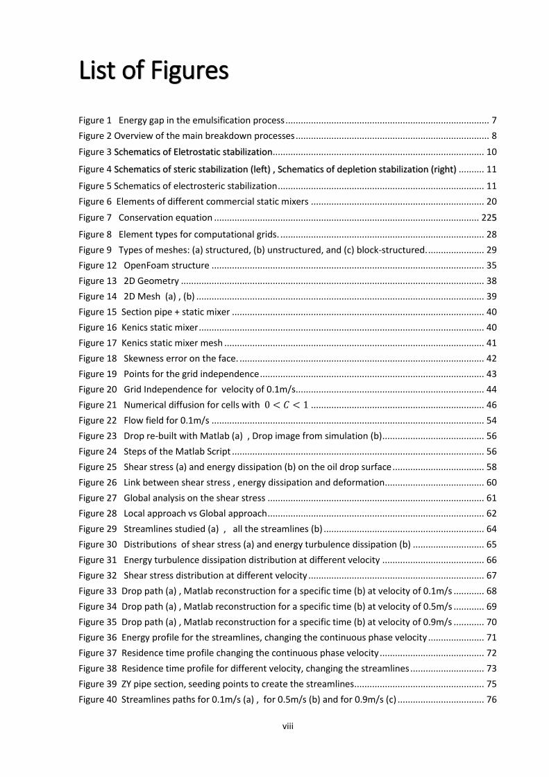
Figure 1 Energy gap in the emulsification process
In Figure 1 the energy gap between the separate phases condition and the dispersed condition
is represented. In the chart, ΔG* is the energetic barrier due to the eventual presence of the
emulsifier that has the role of avoiding the return to the low energy condition. It is a well-known
phenomenon that surfactants, even at low concentration, influence strongly the droplet
formation (Fischer and Erni 2007). They help to control the oil droplet size by reducing the
interfacial tension and decreasing coalescence by affecting interfacial mobility. The drop
formation in the actual process is due mainly to the Kelvin-Helmholtz instability (Kiss, Brenn et
al. 2011), a phenomenon that takes place when two fluids, with different densities, move in
parallel flows (Thomson 1871). This mechanism was also found in spray formation by pre-
filming atomizers (Dorfner et al., 1995).
But several processes relating to the breakdown of emulsions may occur on storage, depending
on:
the particle size distribution and the density difference between the droplets and the
medium; .
the magnitude of the attractive versus repulsive forces, which determines flocculation;
the solubility of the disperse droplets and the particle size distribution, which in turn
determines Ostwald ripening;
The stability of the liquid film between the droplets, which determines coalescence;
and phase inversion.
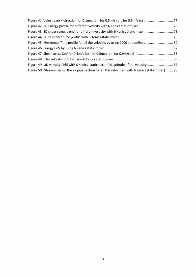
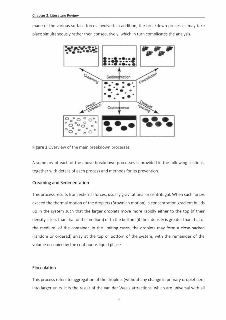
The various breakdown processes are illustrated schematically in Figure 2. The physical
phenomena involved in each breakdown process are not simple, and require an analysis to be
Chapter 2. Literature Review
8
made of the various surface forces involved. In addition, the breakdown processes may take
place simultaneously rather then consecutively, which in turn complicates the analysis.
Figure 2 Overview of the main breakdown processes
A summary of each of the above breakdown processes is provided in the following sections,
together with details of each process and methods for its prevention.
Creaming and Sedimentation
This process results from external forces, usually gravitational or centrifugal. When such forces
exceed the thermal motion of the droplets (Brownian motion), a concentration gradient builds
up in the system such that the larger droplets move more rapidly either to the top (if their
density is less than that of the medium) or to the bottom (if their density is greater than that of
the medium) of the container. In the limiting cases, the droplets may form a close-packed
(random or ordered) array at the top or bottom of the system, with the remainder of the
volume occupied by the continuous liquid phase.
Flocculation
This process refers to aggregation of the droplets (without any change in primary droplet size)
into larger units. It is the result of the van der Waals attractions, which are universal with all

Chapter 2. Literature Review
9
disperse systems. Flocculation occurs when there is not sufficient repulsion to keep the
droplets apart at distances where the van der Waals attraction is weak. Flocculation may be
either ‘strong’ or ‘weak’, depending on the magnitude of the attractive energy involved.
Ostwald Ripening (Disproportionation)
This effect results from the finite solubility (etc.) of the liquid phases. Liquids that are referred
to as being ‘immiscible’ often have mutual solubilities which are not negligible. With emulsions,
which are usually polydisperse, the smaller droplets will have a greater solubility when
compared to larger droplets (due to curvature effects). With time, the smaller droplets
disappear and their molecules diffuse to the bulk and become deposited on the larger droplets.
With time, the droplet size distribution shifts to larger values.
Coalescence
This refers to the process of thinning and disruption of the liquid film between the droplets,
with the result that fusion of two or more droplets occurs to form larger droplets. The limiting
case for coalescence is the complete separation of the emulsion into two distinct liquid phases.
The driving force for coalescence is the surface or film fluctuations; this results in a close
approach of the droplets whereby the van der Waals forces are strong and prevent their
separation.
Phase Inversion
This refers to the process whereby there will be an exchange between the disperse phase and
the medium. For example, an O/W emulsion may with time or change of conditions invert to a
W/O emulsion. In many cases, phase inversion passes through a transition state whereby
multiple emulsions are produced.
Preventing the occurrence of those phenomena is crucial for the long term stability of the
emulsion, in this, adsorbed surfactants exert their role. Since there are always strong, long-
range attractive forces between similar colloidal particles, it is necessary to provide a long range
repulsion between the particles to impart stability.
Stability can be obtained with several mechanisms :
With an electrical double layer (electrostatic or charge stabilization).
With adsorbed or chemically attached polymeric molecules (steric stabilization).
With free polymer in the dispersion medium (depletion stabilization).
Chapter 2. Literature Review
10
Combination of the first two stabilization mechanisms lead to electrosteric stabilization. The
latter two types of stabilization are often realized by the addition of polymers to stabilize
dispersions and are called polymeric stabilization.
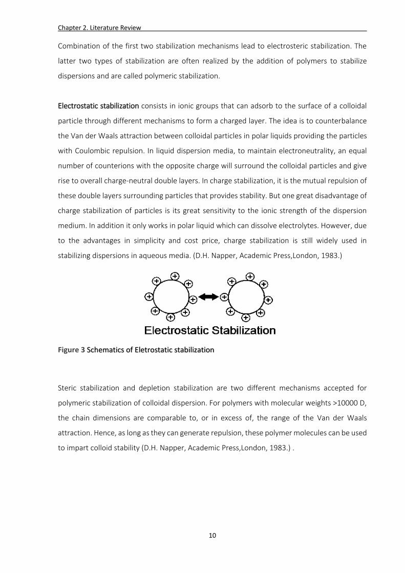
Electrostatic stabilization consists in ionic groups that can adsorb to the surface of a colloidal
particle through different mechanisms to form a charged layer. The idea is to counterbalance
the Van der Waals attraction between colloidal particles in polar liquids providing the particles
with Coulombic repulsion. In liquid dispersion media, to maintain electroneutrality, an equal
number of counterions with the opposite charge will surround the colloidal particles and give
rise to overall charge-neutral double layers. In charge stabilization, it is the mutual repulsion of
these double layers surrounding particles that provides stability. But one great disadvantage of
charge stabilization of particles is its great sensitivity to the ionic strength of the dispersion
medium. In addition it only works in polar liquid which can dissolve electrolytes. However, due
to the advantages in simplicity and cost price, charge stabilization is still widely used in
stabilizing dispersions in aqueous media. (D.H. Napper, Academic Press,London, 1983.)
Figure 3 Schematics of Eletrostatic stabilization
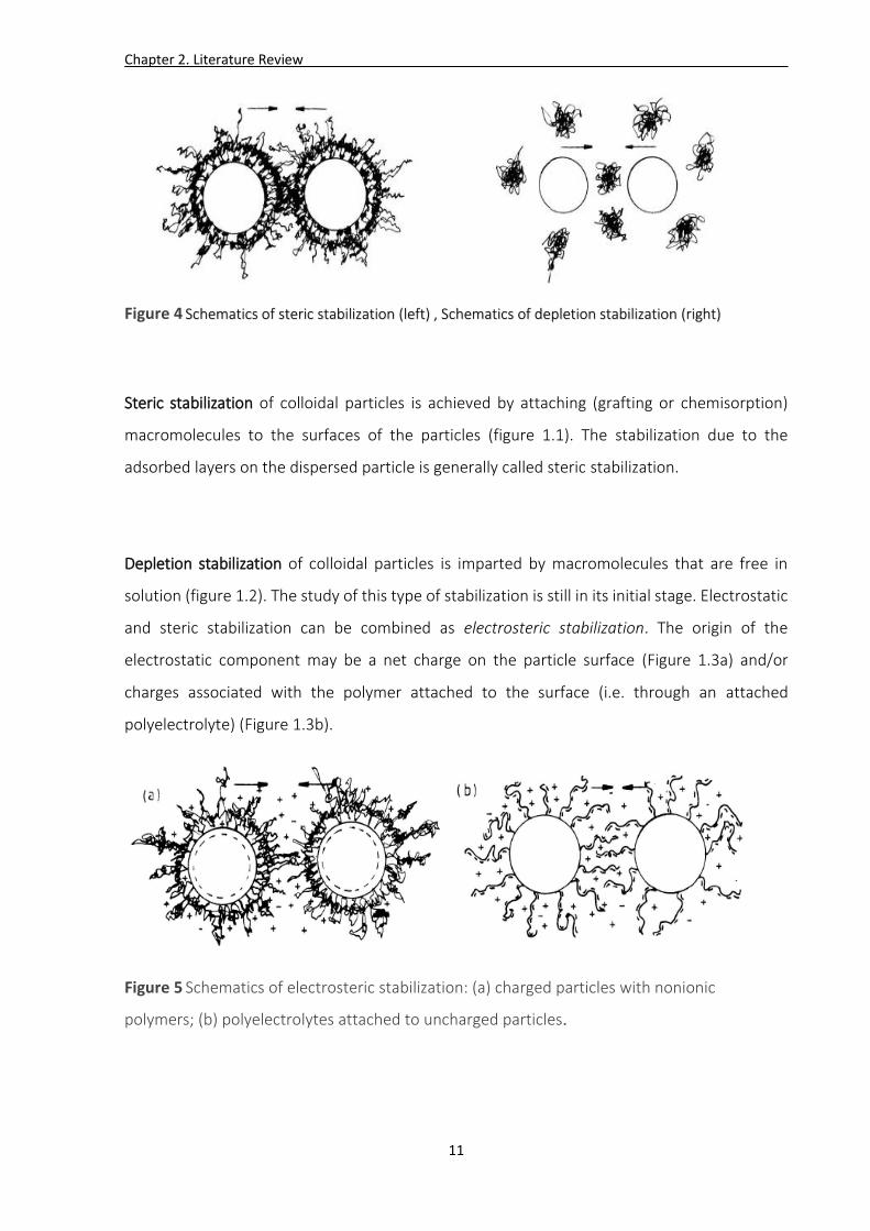
Steric stabilization and depletion stabilization are two different mechanisms accepted for
polymeric stabilization of colloidal dispersion. For polymers with molecular weights >10000 D,
the chain dimensions are comparable to, or in excess of, the range of the Van der Waals
attraction. Hence, as long as they can generate repulsion, these polymer molecules can be used
to impart colloid stability (D.H. Napper, Academic Press,London, 1983.) .
Chapter 2. Literature Review
11
Figure 4 Schematics of steric stabilization (left) , Schematics of depletion stabilization (right)
Steric stabilization of colloidal particles is achieved by attaching (grafting or chemisorption)
macromolecules to the surfaces of the particles (figure 1.1). The stabilization due to the
adsorbed layers on the dispersed particle is generally called steric stabilization.
Depletion stabilization of colloidal particles is imparted by macromolecules that are free in
solution (figure 1.2). The study of this type of stabilization is still in its initial stage. Electrostatic
and steric stabilization can be combined as electrosteric stabilization. The origin of the
electrostatic component may be a net charge on the particle surface (Figure 1.3a) and/or
charges associated with the polymer attached to the surface (i.e. through an attached
polyelectrolyte) (Figure 1.3b).
Figure 5 Schematics of electrosteric stabilization: (a) charged particles with nonionic
polymers; (b) polyelectrolytes attached to uncharged particles.
Chapter 2. Literature Review
12
2.2.3 Droplet breakup mechanism
The prediction and the control of the final drop size of the dispersed phase require a deep
analysis of the droplet breakup mechanisms. Since this difficulty in achieving the satisfying final
dimension, the processes are commonly conducted in turbulent regime. Turbulent particles
breakup has been the subject of an ongoing investigation, beginning with the pioneering work
of Kolmogorov (1949) and Hinze (1955). Many efforts have been done in this field for
understanding the turbulent dispersions in stirred tanks and pipelines (Shinnar 1961, Sleicher
1962, Arai 1977, Calabrese 1986a, Calabrese,
Wang et al. 1986b, Wang and Calabrese 1986b, Berkman and Calabrese 1988, Hesketh, Etchells
et al. 1991, Cabaret, Rivera et al. 2007). Other research has focused on the study of particle
breakup frequency developing models to predict the final drop size distribution (Coulaloglou
and Tavlarides 1977, Konno, Matsunaga et al. 1980, Prince and Blanch 1990, Tsouris and
Tavlarides 1994, Luo and Svendsen 1996, Eastwood, Armi et al. 2004).
In general the principle of break-up can be looked upon as the interaction between two types
of forces (Hinze, 1955). An external disturbing force, induced by the flow field, tries to deform
the droplet and an internal restoring force tries to keep the droplet in its original shape. As a
first approximation the restoring force can be represented by the interfacial tension which is
proportional to σ/d, where σ is the interfacial tension and d the droplet diameter. The
disturbing force, τ, can be either an inertial or a viscous force, exerted by the surrounding
continuous phase on the dispersed droplet. The ratio between the disturbing and the restoring
forces, τd/σ, is often used for the description of the break-up process. Depending on whether
the disturbing force is inertial or viscous, the ratio is called Weber number (We) or Capillary
number (Ca) , respectively. If this ratio exceeds a certain value, the droplet will break up. This
critical number depends on the ratio between the viscosities of the dispersed and continuous
phases and the geometry of the flow field around the droplet (Janssen, 1993).

Chapter 2. Literature Review
13
2.2.3.1 Breakup in a laminar flow
Viscous shear forces in the continuous phase cause a velocity gradient around the interface
that deforms the fluid particle and can lead to breakup. Shear stresses also appear due to the
wake effect downstream of an obstacle. The canonical laminar flow fields are simple shear flow
and, for the elongational component, uniaxial, planar or equibiaxialflow (Windhab et al., 2005).
This means that in laminar flow two different cases should be analysed:
Simple shear: when the velocity gradient and the flow direction are parallel;
Simple extensional: when the elongation is present and the stretching is on a single
axis.
In simple shear flow the deforming viscous stresses 𝜏𝑣 acting on the surface of emulsion drops
are generated proportional to the acting shear rates and the related viscosity of the continuous
fluid phase: 𝜏𝑣 = 𝜇𝑐 ∙ |𝛾|̇ ;
With 𝜇𝑐 the continuous-phase viscosity and |𝛾|̇ the shear rate. The capillary pressure PL acting
against the deforming stresses is given by the Laplace equation leading to a spherical drop:
𝐏𝐋 =𝟒𝛔
𝐝 (3)
with 𝜎 the interfacial tension and d the diameter of the spherical droplet. The dimensionless
stress ratio 𝜏𝑣
𝑃𝐿 is denoted by the shear capillary number 𝐶𝑎𝑆 :
𝐂𝐚𝐒 =𝛍𝐜∙|𝛄|̇ ∙𝐝
𝟐𝛔 (4)
with d the droplet size. Drop breakup occurs if the critical capillary number is exceeded. Hence
the maximum drop diameter surviving under shear flow conditions ds max is given by the
critical shear capillary number 𝐶𝑎𝑆 from Eq. (4) as :
𝐝𝐦𝐚𝐱 =𝟐∙𝐂𝐚𝐂𝐫
𝐒 ∙𝛔
𝛍𝐜∙|𝛄|̇ (5)
As the breakup proceeds with the flow, of course the 𝑑𝑚𝑎𝑥 obtained from Eq. (5) is valid if the
residence time of the drop in the shear breakage zone is much greater than the deformation
Chapter 2. Literature Review
14
time scale of the drop. Note that recent numerical simulations (Windhab et al., 2005) can
reproduce the interface deformation and splitting at the scale of a few numbers of drops.
In presence of elongational flow ( laminar flow) , drops can also be deformed when the fluid
elements accelerate and induce a normal strain and stress. The highest accelerating rates in
the flow controls 𝑑𝑚𝑎𝑥 . The drops are convected along the streamlines, and so from a
Lagrangian point of view the drops experience a non-uniform strain rate due to the spatial
heterogeneity of the velocity field. The analysis developed for the case of shear flows is also
valid for the extensional laminar steady flows, in which the extensional rate 𝜀̇ is included in the
definition of the capillary number in place of the shear rate. In practice, the generalized shear
rate can be used (second invariant of the strain rate tensor) in the capillary number, as it takes
into account both the extensional and shear components.
𝐶𝑎𝑒 =𝜇𝑐∙|𝜀|̇ ∙𝑑
2𝜎 (6)
With |𝜀|̇ the extensional rate.
As for the shear stress case, from Eq. (6), the maximum drop diameter due to elongation
𝑑𝑚𝑎𝑥 can be expressed as :
𝑑𝑚𝑎𝑥 =2∙𝐶𝑎𝐶𝑟
𝑒 ∙𝜎
𝜇𝑐∙|𝜀|̇ (7)
Eq. (7) can be used to predict 𝑑𝑚𝑎𝑥, with the same remark onthe drop residence time in the
high-elongation rate zone.
2.2.3.2 Breakup in a turbulence flow
In a turbulent flow field, the breakup of fluid particles is caused mainly by turbulent pressure
fluctuations on the drop surface, sometime called particle-eddy collisions. The particle can be
assumed to modify its spherical form with the fluctuation of the surrounding fluid. When the
amplitude of the oscillation is close to that required to make the particle surface unstable, it
starts to deform and fragments into two (or more) daughter particles. The breakup mechanism
can then be expressed as a balance between the dynamic pressure 𝜏𝑖 and the capillary force
𝜏𝑠 . The viscous stresses of the fluid inside the particle are usually neglected in a coarse

Chapter 2. Literature Review
15
approach. Whether or not the particle breaks depends on the extent of the deformation,
characterized by the Weber number 𝑊𝑒 =𝜏𝑖
𝜏𝑠 . Concerning this criterion for breakup, Liao and
Lucas (2009) distinguish some mechanisms, the most significant being that the turbulent kinetic
energy of the particle is greater than a critical value (Chatzi and Kiparissides, 1992;
Coulaloglouand Tavlarides, 1977) and that the turbulent kinetic energy of the eddy is greater
than a critical value (Martínez-Bazán etal., 1999a,b; Luo and Svendsen, 1996; Tsouris and
Tavlarides,1994). The critical energy is arbitrarily defined by the above authors as the surface
energy of the parent particle (Martínez-Bazán et al., 1999a,b), the increase in surface energy
before and after breakup (Luo and Svendsen, 1996), or the mean value of the surface energy
increase for breakup into two equal-size daughters and into a smaller and a larger one (Tsouris
andTavlarides, 1994).
In turbulent flow fields, all flow parameters fluctuate locally, resulting in an eddy size
distribution ranging from the macroscale L to the Kolmogorov length scale 𝜆𝐾. The Kolmogorov
and Hinze theory, suggested independently by Kolmogorov (1949) and Hinze (1955), is based
on the idea of an energy cascade. It is the main contribution to a physical understanding and
provides a universal model for droplet breakup in turbulent flow. The Kolmogorov scale 𝜆𝐾 is
characterized by a Reynolds number of about unity :
𝝀𝑲 = 𝝂𝑪𝟑/𝟒
∙ 𝜺−𝟏/𝟒 (8)
where 𝜈𝐶 is the kinematic viscosity of the continuous phase and ε the energy dissipation rate
per mass unit. The size of the largest stable drop in the emulsion is determined by the
equilibrium between the turbulent pressure fluctuations, which tend to deform and break up
the drop, and the surface tension, which resists these deformations and holds the drop
together. From previous considerations, the ratio of these two constraints defines the droplet
Weber number:
We =ρc∙δu(d)2̅̅ ̅̅ ̅̅ ̅̅ ̅̅ ∙d
σ (9)
where 𝜌𝑐 is the continuous phase density and δu(d)2 the spatial longitudinal autocorrelation
of instantaneous velocities at the distance d equal to the drop diameter. In the inertial field for
isotropic turbulence in the drop length scale, δu(d)̅̅ ̅̅ ̅̅ ̅̅ 2 is given by Batchelor (1953) as:
δu(d)2̅̅ ̅̅ ̅̅ ̅̅ ̅ = CK ∙ ε2/3 ∙ d2/3 (10)

Chapter 2. Literature Review
16
where CK is known as the Kolmogorov constant in physical space (there is a related constant
in spectral space). As previously mentioned, droplet breakup occurs when the Weber number
reaches a critical value We cr. So the maximum diameter 𝑑𝑚𝑎𝑥 of drops that resist further
breakup by the turbulent fluctuations is obtained as:
𝐝𝐦𝐚𝐱 = (𝐖𝐞𝐜𝐫
𝐂𝐊)
𝟑/𝟓 ∙ (
𝛔
𝛒)𝟑/𝟓 ∙ 𝛆−𝟐/𝟓 (11)
This approach leads to the conclusion that the viscosity forces in the dispersed phase are
negligible, a statement that could be justified for drop sizes much larger than the Kolmogorov
length scale.
The application of this model to “non-coalescing”systems has been tested over a wide range of
processes: stirred vessels, emulsifiers with ultrasound, and homogenizers. Many authors
(Eastwood et al., 2004; Hesketh et al., 1991; Martínez-Bazán et al., 1999a; Risso and Fabre,
1998; Streiff et al., 1997) report good predictions of the maximum droplet diameter, despite
some discrepancies in the constant value (Wecr/𝐶𝑘)3/5.
2.3 Mixing equipment
2.3.1 Introduction
“Characterizing mixing in industrial processes is an important issue for various economic and
environmental considerations since it governs byproduct effluents and consequently process
efficiency. (Anxionnaz et al., 2008; Lobry et al., 2011;Stankiewicz and Moulijn, 2000) “
The mixing of liquids is a unit operation in which two or more miscible or immiscible liquids are
mixed together to reach a certain degree of homogeneity or dispersion (Paul 2003). Mixing is a
common operation for the manufacture of a wide range of products such as food, personal
care, home care and catalysts industry. When the mixing involves immiscible fluids the
operation is called dispersion. Stirred vessels, rotor-stator mixers, static mixers, decanters,
settlers, centrifuges, homogenizers, extraction columns, and electrostatic coalescers are
examples of industrial process equipment used to handle liquid-liquid systems. All these
operations can be classified as batch or continuous processes (Hall, Cooke et al. 2011). In batch

Chapter 2. Literature Review
17
processes, stirred tanks and similar devices are used to blend fluids, employing an impeller for
generating the fluid motion. The amount of time required to reach the degree of homogeneity
desired is known as the blend time or residence time, which is the time spent by the fluid inside
the tank before reaching the desired level of mixing. Static mixers and similar devices are used
for continuous processes where fluids are pumped through mixing elements installed inside
pipes. In the following table the main characteristics of static mixers compared with stirred
tanks are reported (Thakur, Vial et al. 2003).
Static Mixer CSTR
Small space requirement Large space requirement
Low equipment cost High equipment cost
No power required except pumping High power consumption
No moving parts except pump Agitator drive and seals
Short residence times Long residence times
Approaches plug flow Exponential distribution of residence times
Good mixing at low shear rates Locally high shear rates can damage
sensitive materials
Fast product grade changes Product grade changes may generate waste
Self-cleaning, interchangeable mixers
or disposable mixers
Large vessels to be cleaned
Table 2 Comparison between features of static mixer and stirred tank
2.3.2 Mixing of immiscible liquids in Stirred Tank
Stirred vessels are among the most commonly used pieces of equipment in the chemical and
biochemical processes. They are used for the homogenization of single or several phases. There
are at least two kinds of agitation commonly employed in stirred vessels: pneumatic and
mechanical. The former type uses an air stream in order to achieve bulk mixing. The latter
method is based on the use of rotating impellers driven usually by electrical motors. Mixing and
contacting in agitated tanks can be accomplished in continuous, batch, or fed-batch mode. A
good mixing result is important for minimizing investment and operating costs, providing high
yields when mass transfer is limiting, and thus enhancing profitability. Processing with
mechanical mixers occurs under either laminar or turbulent flow conditions, depending on the
impeller Reynolds number, defined as Re = ρND2/μ.
Chapter 2. Literature Review
18
Stirred vessels are still powerful tools in process industry and find vast applications especially
for process in highly viscous products (Aubin and Xuereb, 2006; Cabaretet al., 2007). Numerous
recent studies investigate their hydro-dynamics with Newtonian as well as rheologically
complex fluids (Alliet-Gaubert et al., 2006; Aubin et al., 2000, 2001;Fangary et al., 2000; Torré
et al., 2007). New impeller and mixing vessel configurations and innovative operating methods
are being introduced to enhance their mixing efficiency, safety, and overall productivity (Aubin
et al., 2006; Fentiman et al.,1998; Torré et al., 2008).
The quality of mixing mainly depends upon the relative distribution of mean and turbulent
kinetic energy. Power draw is a very important variable in chemical and bioprocess
engineering. It is defined as the amount of energy necessary in a period of time, in order to
generate the movement of the fluid within a container (e.g. bioreactor, mixing tank, chemical
reactor, etc.) by means of mechanical or pneumatic agitation. The costs associated with power
draw contribute significantly to the overall operation costs of industrial plants. Therefore, it is
desired that the mixing process is performed efficiently and with a minimum expense of energy
required to achieve the objective established a priori (Bader, 1987). Power draw influences
heat and mass transfer processes, mixing and circulation times. Power draw has been used as
a criterion for process scale-up and bioreactor design (Charles, 1985). Commonly, it is referred
as the volumetric power draw (P=V).
In view of such an immense importance of the knowledge of quality of flow, vigorous research
efforts have been made during the last 50 years using various flow measurement techniques
and computational fluid dynamics (CFD). The on going demand for the improved impeller
designs usually comes from the users of industrial mixing equipment when the vessels are to
be designed for new plants or improvement in the existing design is desired for enhancing
quality, capacity, process efficiency and energy efficiency.
2.3.3 Mixing of immiscible liquids in Static Mixer
Static mixers, also known as motionless mixers, have become standard equipment in the
process industries. However, new designs are being developed and new applications are being
explored. Static mixers are employed inline in a once-through process or in a recycle loop where
they supplement or even replace a conventional agitator. Their use in continuous processes is
Chapter 2. Literature Review
19
an attractive alternative to conventional agitation since similar and sometimes better
performance can be achieved at lower cost. Motionless mixers typically have lower energy
consumptions and reduced maintenance requirements because they have no moving parts.
They offer a more controlled and scaleable rate of dilution in fed batch systems and can provide
homogenization of feed streams with a minimum residence time. They are available in most
materials of construction.
Although static mixers did not become generally established in the process industries until the
1970s, the patent is much older. An 1874 patent describes a single element, multilayer
motionless mixer used to mix air with a gaseous fuel (Sutherland, 1874). Nowadays there are
approximately 2000 US patents and more than 8000 literature articles that describe motionless
mixers and their applications. More than 30 commercial models are currently available. The
prototypical design of a static mixer is a series of identical, motionless inserts that are called
elements and that can be installed in pipes, columns or reactors. The purpose of the elements
is to redistribute fluid in the directions transverse to the main flow, i.e. in the radial and
tangential directions. The effectiveness of this redistribution is a function of the specific design
and number of elements. Commercial static mixers have a wide variety of basic geometries and
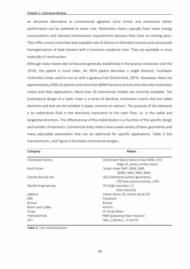
many adjustable parameters that can be optimized for specific applications. Table 3 lists
manufacturers, and Figure 6 illustrates commercial designs.
Company Mixers Chemineer-Kenics Chemineer-Kenics Kenics mixer (KM), HEV
(high ef_ciency vortex mixer) Koch-Sulzer Sulzer mixer SMF, SMN, SMR,
SMRX, SMV, SMX, SMXL Charles Ross & Son ISG (interfacial surface generator),
LPD (low pressure drop), LLPD Wymbs Engineering HV (high viscosity), LV
(low viscosity) Lightnin Inliner Series 45, Inliner Series 50 EMI Cleveland Komax Komax Brann and Lubbe N-form Toray Hi-Toray Mixer Prematechnik PMR (pulsating mixer reactor) UET Heli_o (Series, I, II and III)
Table 3 Lists manufacturers
Chapter 2. Literature Review
20
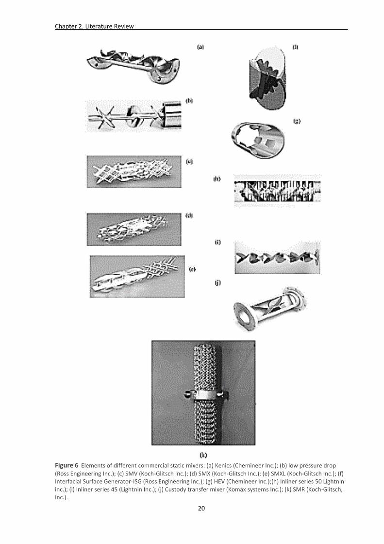
Figure 6 Elements of different commercial static mixers: (a) Kenics (Chemineer Inc.); (b) low pressure drop
(Ross Engineering Inc.); (c) SMV (Koch-Glitsch Inc.); (d) SMX (Koch-Glitsch Inc.); (e) SMXL (Koch-Glitsch Inc.); (f) Interfacial Surface Generator-ISG (Ross Engineering Inc.); (g) HEV (Chemineer Inc.);(h) Inliner series 50 Lightnin inc.); (i) Inliner series 45 (Lightnin Inc.); (j) Custody transfer mixer (Komax systems Inc.); (k) SMR (Koch-Glitsch, Inc.).

Chapter 2. Literature Review
21
Mixing operations are essential in the process industries. They include the classical mixing of
miscible fluids in single-phase flow as well as heat transfer enhancement, dispersion of gas into
a liquid continuous liquid phase, dispersion of an immiscible organic phase as drops in a
continuous aqueous phase, three-phase contacting and mixing of solids. Static mixers are now
commonly used in the chemical and petrochemical industries to perform continuous
operations. They have also found applications in the pharmaceutical, food engineering and pulp
and paper industries .
In laminar flows, static mixers divide and redistribute streamlines in a sequential fashion using
only the energy of the flowing fluid. In turbulent flows, they enhance turbulence and give
intense radial mixing, even near the wall. In both cases, they can significantly improve heat and
mass transfer operations.
Three different stages are introduced to describe the mixing mechanism: macromixing,
mesomixing and micromixing (Fournier, Falk et al. 1996, Bałdyga and Bourne 1999). In all these
cases, the key parameters to compare the different available static mixer at the same
performance (drop size distribution) are the energy consumption or pressure drop and the
number of elements necessary.
The pressure drop in a static mixer of fixed geometry is expressed as the ratio of the pressure
drop through the mixer to the pressure drop through the same diameter and length of open
pipe , by using a K factor (KL for laminar and KT for turbulent flow) determined empirically.
∆PSM = {
KL ∙ ∆PEmptyPipe
KT ∙ ∆PEmptyPipe
(12)
Where the standard pressure drop for an empty smooth pipe are:
∆P = 4f ∙L
D∙ ρ ∙
V2
2 (13)
And the Fanning friction factor is given by the Blasius equation for turbulent flow:
f =0.079
Re0.25 (14)
Chapter 2. Literature Review
22
and in laminar flow by:
f =16
Re (15)
In Tables 7-5 values of KL and KT are given. These values are considered good to about 15%.
Device 𝐾𝐿 𝐾𝑇 Empty pipe 1 1 KMS 6.9 150 SMX 37.5 500 SMXL 7.8 100 SMR 46.9 -
SMV - 100-200
Table 4 Values of KL and KT for different static mixer (Streiff 1997)
Most vendors have more accurate correlations that take into account a slight Reynolds number
effect in transitional and turbulent flow, and the volume fraction occupied by the mixer, which
varies with mixer diameter and pressure rating. A more detailed approach is necessary for some
designs that have the option for variable but similar geometry. For the most accurate pressure
drop predictions, the manufacturer should always be consulted.
There is still, of course, substantial room for further improvement and new designs and
principles for these devices. Even the most widely studied geometries can still be further
optimized. Fouling resistance, corrosion, maintenance, and cleaning operations are at present
problems in such devices. Academia seems overly obsessed with theoretical gains in mixing and
heat transfer, and the tools to address technical complications in the implementation and
production phases are still immature and need extensive development. Moreover, laboratory-
scale optimization processes are leading to new designs but sometimes it can take years for
research prototypes to become available in the markets, if ever.

Chapter 2. Literature Review
23
2.4 Computational fluid dynamic for mixing
2.4.1 Introduction
Computational fluid dynamics (CFD) is the numerical simulation of fluid motion. While the
motion of fluids in mixing is an obvious application of CFD, there are hundreds of others,
ranging from blood flow through arteries, to supersonic flow over an airfoil, to the extrusion of
rubber in the manufacture of automotive parts. While in 1975 numerical results were only
making their entrance into the arena of fluid flow and heat/mass transfer and they were not
considered serious competition to experimental data (Chapman et al. 1975), thirty years later,
computational projects and results constitute the major source of useful and reliable
information in most engineering and physical disciplines. The combination of significant
improvements and advances in computational speed and accuracy, and the affordability of
computational power have prompted most scientists to use numerical methods for the studies
on the flow and heat/mass transfer processes associated with particles, bubbles and drops and,
thus, develop the new field of Computational Fluid Dynamics (CFD). Numerous models and
solution techniques have been developed over the years to help describe a wide variety of fluid
motion. The fundamental equations for fluid flow are presented in detailed in the following
paragraphs, but before advantages of CFD in obtaining scientific information rather than
experimental methods are given :
The rapid development of CFD methods has improved significantly the accuracy and
reliability of the final results.
The cost of CFD calculations in the simulation of realistic systems and conditions has
dropped dramatically, while the cost of experimentation has constantly increased.
CFD generates complete and easily accessible information. The results of a simulation
may be viewed in different ways and from different points, thus providing the
researcher with a complete depiction of the object of study.
CFD has the ability to model and simulate idealized or desired conditions for a specific
variable or effect, which are difficult or impossible to achieve in practice
Chapter 2. Literature Review
24
2.4.2 Conservation Equations
If a small volume, or element of fluid in motion is considered, two changes to the element will
probably take place: (1) the fluid element will translate and possibly rotate in space, and (2) it
will become distorted, either by a simple stretching along one or more axes or by an angular
distortion that causes it to change shape. The process of translation is often referred to as
convection, and the process of distortion is related to the presence of gradients in the velocity
field and a process called diffusion. In the simplest case, these processes govern the evolution
of the fluid from one state to another. In more complicated systems, sources can also be
present that give rise to additional changes in the fluid.
Many of the processes such as those that are involved in the description of generalized fluid
motion are described by a set of conservation or transport equations. These equations track,
over time, changes in the fluid that result from convection, diffusion, and sources or sinks of
the conserved or transported quantity. Furthermore, these equations are coupled, meaning
that changes in one variable (say, the temperature) can give rise to changes in other variables
(say, the pressure). The conservation equations are:
Continuity equation
Momentum equation
Species equation
Energy equation
2.4.2.1 Continuity Equation
The continuity equation is a statement of conservation of mass. To understand its origin,
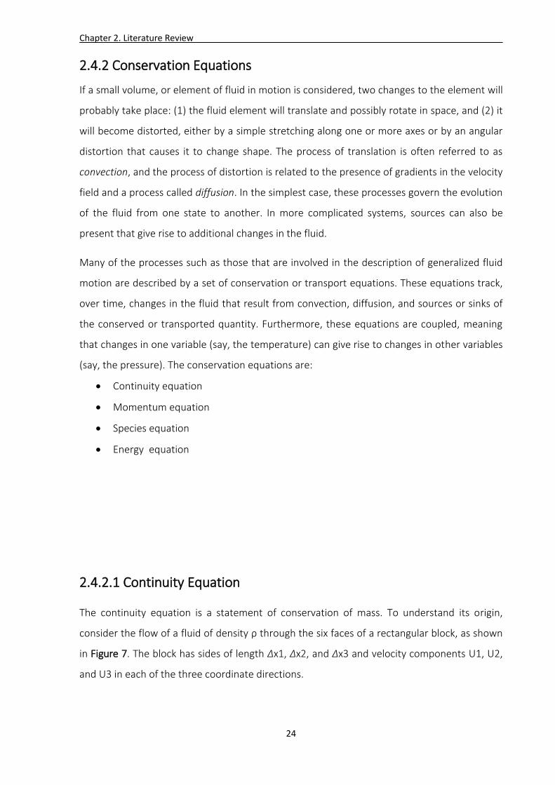
consider the flow of a fluid of density ρ through the six faces of a rectangular block, as shown
in Figure 7. The block has sides of length Δx1, Δx2, and Δx3 and velocity components U1, U2,
and U3 in each of the three coordinate directions.
Chapter 2. Literature Review
25
Figure 7 A rectangular volume with inflow and outflow can be used to illustrate a conservation equation.
To ensure conservation of mass, the sum of the mass flowing through all six faces must be zero:
ρ(U1,out − U1,in) ∙ (∆x2 ∙ ∆x3) + ρ(U2,out − U2,in) ∙ (∆x1 ∙ ∆x3)
+ ρ(U3,out − U3,in) ∙ (∆x1 ∙ ∆x2) = 0 (16)
Dividing through by (Δx1Δx2Δx3) the equation can be written as :
ρ ∙∆U1
∆x1+ ρ ∙
∆U2
∆x2+ ρ ∙
∆U3
∆x3= 0 (17)
or, in differential form :
ρ ∙∂U1
∂x1+ ρ ∙
∂U2
∂x2+ ρ ∙
∂U3
∂x3= 0 (18)
For more general cases, the density can vary in time and in space, and the continuity equation
takes on the more familiar form :
∂ρ
∂t+
∂(ρUi)
∂xi = 0 (19)
2.4.2.2 Momentum Equation
The momentum equation is a statement of conservation of momentum in each of the three
component directions. The three momentum equations are collectively called the Navier–
Stokes equations. In addition to momentum transport by convection and diffusion, several
momentum sources are also involved:
Chapter 2. Literature Review
26
∂(ρUi)
∂t+
∂(ρUiUj)
∂xj = −
∂p
∂xi+
∂
∂xj[μ (
∂Ui
∂xj+
∂Uj
∂xi−
2
3∙
∂Uk
∂xk∙ δij)] + ρg + Fi (20)
In eq. (20) the convection terms are on the left. The terms on the right-hand side are the
pressure gradient, a source term; the divergence of the stress tensor, which is responsible for
the diffusion of momentum; the gravitational force, another source term; and other
generalized forces (source terms), respectively.
2.4.2.3 Species Equation The species equation is a statement of conservation of a single specie. Multiple-species
equations can be used to represent fluids in a mixture with different physical properties.
Solution of the species equations can predict how different fluids mix, but not how they will
separate. For the species i , the conservation equation is for the mass fraction of that species,
mi, and has the following form:
∂(ρmi)
∂t+
∂(ρUimi)
∂xi = −
∂(Ji,i)
∂xi+ Ri + Si (21)
In eq. (21), Ji,i is the i component of the diffusion flux of species i in the mixture. For laminar
flows, Ji,i is related to the diffusion coefficient for the species and local concentration gradients
(Fick’s law of diffusion). For turbulent flows, Ji,i includes a turbulent diffusion term, which is a
function of the turbulent Schmidt number. Ri is the rate at which the species is either consumed
or produced in one or more reactions, and Si is a general source term for species. When two or
more species are present, the sum of the mass fractions in each cell must add to 1.0. For this
reason, if there are n species involved in a simulation, only n − 1 species equations need to be
solved. The mass fraction of the nth species can be computed from the required condition:
∑ mi = 0ni=! (22)
2.4.2.4 Energy Equation
Heat transfer is often expressed as an equation for the conservation of energy, typically in the
form of static or total enthalpy. Heat can be generated (or extracted) through many
mechanisms, such as wall heating (in a jacketed reactor), cooling through the use of coils, and
Chapter 2. Literature Review
27
chemical reaction. In addition, fluids of different temperatures may mix in a vessel, and the
time for the mixture to come to equilibrium may be of interest. The equation for conservation
of energy (total enthalpy) is :
∂(ρE)
∂t+
∂[Ui(ρE+p)]
∂xi=
∂
∂xi[Keff
∂T
∂xi+ ∑ hjJi,j + Ui(τij)eff] + Sh (23)
In this equation, the energy, E, is related to the static enthalpy, h, through the following
relationship involving the pressure, p, and velocity magnitude, U:
E = h −p
ρ+
U2
2 (24)
The first term on the right-hand side of eq. (24) represents heat transfer due to conduction, or
the diffusion of heat, where the effective conductivity, keff, contains a correction for turbulent
simulations. The second term represents heat transfer due to the diffusion of species, where
Jj,i is the diffusion flux. The third term involves the stress tensor, (τij)eff, a collection of velocity
gradients, and represents heat loss through viscous dissipation. The fourth term is a general
source term that can include heat sources due to reactions, radiation, or other processes.
2.4.3 Numerical Methods
The differential equations presented above describe the continuous movement of a fluid in
space and time. To be able to solve those equations numerically, all aspects of the process need
to be discretized, or changed from a continuous to a discontinuous formulation. For example,
the region where the fluid flows needs to be described by a series of connected control
volumes, or computational cells. The equations themselves need to be written in an algebraic
form. Advancement in time and space needs to be described by small, finite steps rather than
the infinitesimal steps that are so familiar to students of calculus. All of these processes are
collectively referred to as discretization. In the next paragraphs, discretization of the domain,
or grid generation, and discretization of the equations are presented in detail.
Chapter 2. Literature Review
28
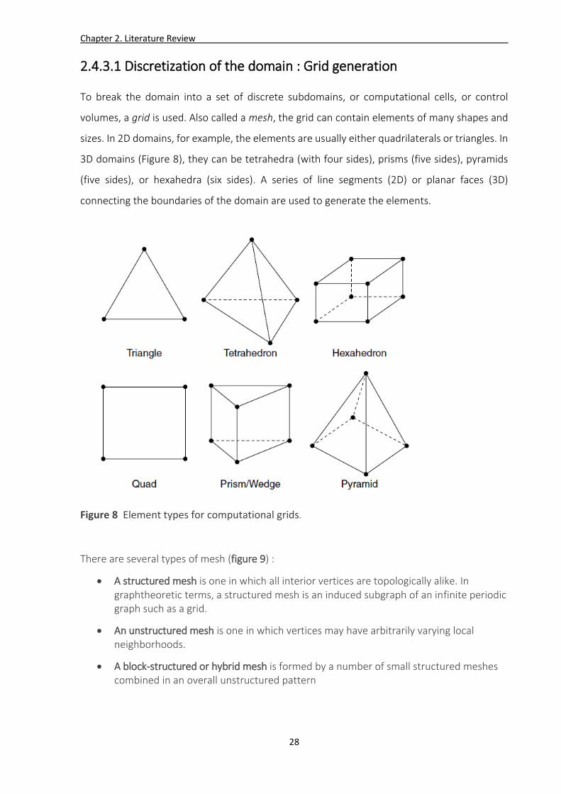
2.4.3.1 Discretization of the domain : Grid generation
To break the domain into a set of discrete subdomains, or computational cells, or control
volumes, a grid is used. Also called a mesh, the grid can contain elements of many shapes and
sizes. In 2D domains, for example, the elements are usually either quadrilaterals or triangles. In
3D domains (Figure 8), they can be tetrahedra (with four sides), prisms (five sides), pyramids
(five sides), or hexahedra (six sides). A series of line segments (2D) or planar faces (3D)
connecting the boundaries of the domain are used to generate the elements.
Figure 8 Element types for computational grids.
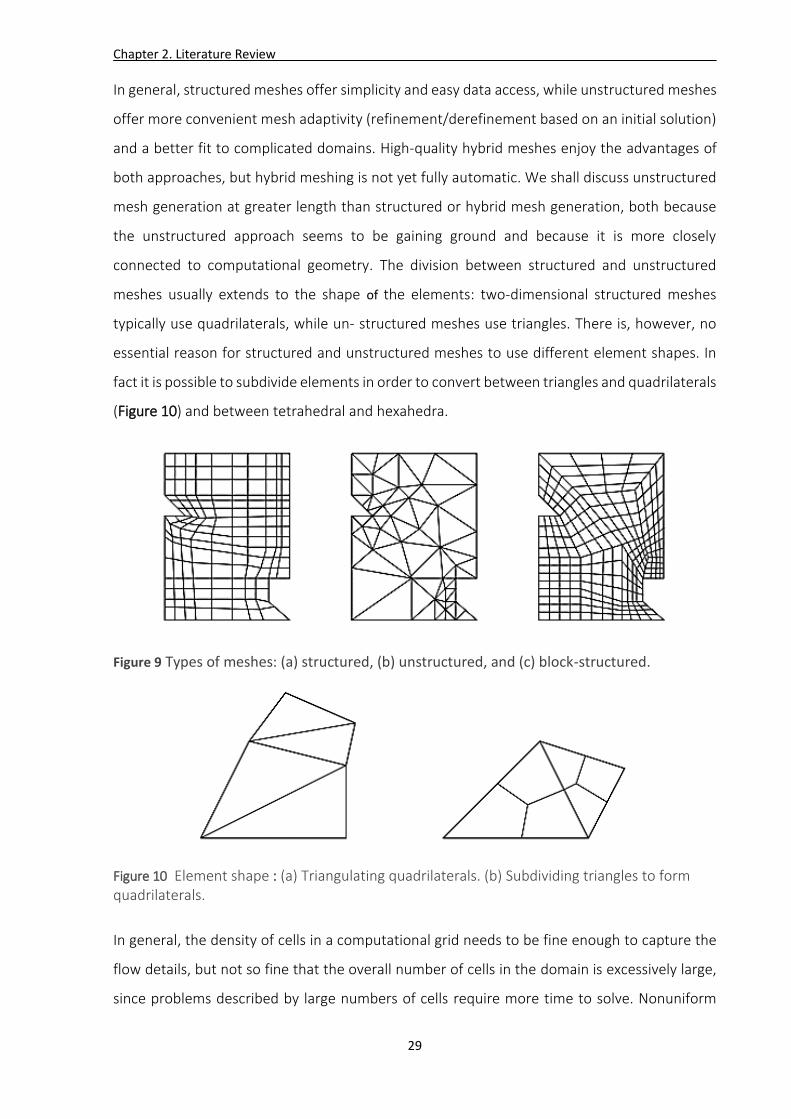
There are several types of mesh (figure 9) :
A structured mesh is one in which all interior vertices are topologically alike. In graphtheoretic terms, a structured mesh is an induced subgraph of an infinite periodic graph such as a grid.
An unstructured mesh is one in which vertices may have arbitrarily varying local neighborhoods.
A block-structured or hybrid mesh is formed by a number of small structured meshes combined in an overall unstructured pattern
Chapter 2. Literature Review
29
In general, structured meshes offer simplicity and easy data access, while unstructured meshes
offer more convenient mesh adaptivity (refinement/derefinement based on an initial solution)
and a better fit to complicated domains. High-quality hybrid meshes enjoy the advantages of
both approaches, but hybrid meshing is not yet fully automatic. We shall discuss unstructured
mesh generation at greater length than structured or hybrid mesh generation, both because
the unstructured approach seems to be gaining ground and because it is more closely
connected to computational geometry. The division between structured and unstructured
meshes usually extends to the shape of the elements: two-dimensional structured meshes
typically use quadrilaterals, while un- structured meshes use triangles. There is, however, no
essential reason for structured and unstructured meshes to use different element shapes. In
fact it is possible to subdivide elements in order to convert between triangles and quadrilaterals
(Figure 10) and between tetrahedral and hexahedra.
Figure 9 Types of meshes: (a) structured, (b) unstructured, and (c) block-structured.
Figure 10 Element shape : (a) Triangulating quadrilaterals. (b) Subdividing triangles to form quadrilaterals.
In general, the density of cells in a computational grid needs to be fine enough to capture the
flow details, but not so fine that the overall number of cells in the domain is excessively large,
since problems described by large numbers of cells require more time to solve. Nonuniform

Chapter 2. Literature Review
30
grids of any topology can be used to focus the grid density in regions where it is needed and to
allow for expansion in other regions. In laminar flows, the grid near boundaries should be
refined to allow the solution to capture the boundary layer flow detail. For turbulent flows, it is
customary to use a wall function in the near-wall regions. This is due to the fact that the
transport equation for the eddy dissipation has a singularity at the wall.
2.4.3.2 Discretization of the Equations
Several methods have been employed over the years to solve the Navier–Stokes equations
numerically, including the finite difference, finite element, spectral element, and finite volume
methods. The focus of this paragraph is on the finite volume method, which is described in
detail below. To illustrate the discretization of a typical transport equation using the finite
volume formulation (Patankar, 1980; Versteeg and Malalasekera, 1995), a generalized scalar
equation can be used. The scalar equation has the form :
𝜕(𝜌𝜙)
𝜕𝑡+
𝜕(𝜌𝑈𝑖𝜙)
𝜕𝑥𝑖=
𝜕
𝜕𝑥𝑖(𝛤
𝜕(𝜙)
𝜕𝑥𝑖) + 𝑆′ (25)
The parameter 𝚪 is used to represent the diffusion coefficient for the scalar φ. If φ is one of the
components of velocity, for example, 𝚪 would represent the viscosity. All sources are collected
in the term S’. The control volume has a node, P, at its center where all problem variables are
stored. The transport equation describes the flow of the scalar φ into and out of the cell through
the cell faces. To keep track of the inflow and outflow, the four faces are labeled with lowercase
letters representing the east, west, north, and south borders. The neighboring cells also have
nodes at their centers, and these are labeled with the capital letters E, W, N, and S. For the
purpose of this example, flow in the one dimensional row of cells shown in Figure 11-b is
considered.
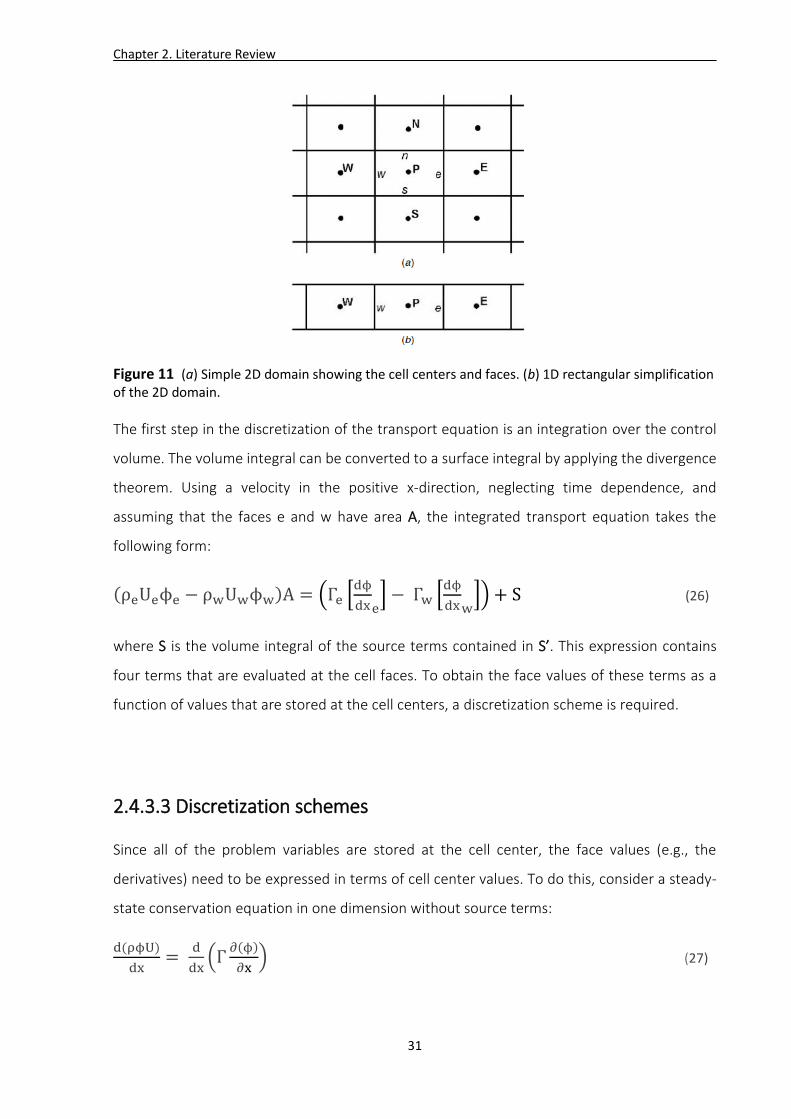
Chapter 2. Literature Review
31
Figure 11 (a) Simple 2D domain showing the cell centers and faces. (b) 1D rectangular simplification of the 2D domain.
The first step in the discretization of the transport equation is an integration over the control
volume. The volume integral can be converted to a surface integral by applying the divergence
theorem. Using a velocity in the positive x-direction, neglecting time dependence, and
assuming that the faces e and w have area A, the integrated transport equation takes the
following form:
(ρeUeϕe − ρwUwϕw)A = (Γe [dϕ
dxe] − Γw [
dϕ
dxw]) + S (26)
where S is the volume integral of the source terms contained in S’. This expression contains
four terms that are evaluated at the cell faces. To obtain the face values of these terms as a
function of values that are stored at the cell centers, a discretization scheme is required.
2.4.3.3 Discretization schemes
Since all of the problem variables are stored at the cell center, the face values (e.g., the
derivatives) need to be expressed in terms of cell center values. To do this, consider a steady-
state conservation equation in one dimension without source terms:
d(ρϕU)
dx=
d
dx(Γ
∂(ϕ)
∂x) (27)

Chapter 2. Literature Review
32
This equation can be solved exactly. On a linear domain that extends from x = 0 to x = L,
corresponding to the locations of two adjacent cell nodes, with 𝜙 = 𝜙𝑜 at x = 0 and 𝜙 = 𝜙𝐿 at
x = L, the solution for φ at any intermediate location (such as the face) has the form :
𝜙 = 𝜙𝑜 + (𝜙𝐿 − 𝜙𝑜) ∙exp (𝑃𝑒(
𝑥
𝐿)−1)
exp (𝑃𝑒−1) (28)
The Peclet number, Pe, appearing in this equation is the ratio of the influence of convection to
that of diffusion on the flow field:
𝑃𝑒 =𝜌𝑈𝐿
Γ (29)
Depending on the value of the Peclet number, different limiting behavior exists for the variation
of φ between x = 0 and x = L. These limiting cases are discussed below, along with some more
rigorous discretization or differencing schemes that are in popular use today. The principle
discretization schemes are :
Central Differencing Scheme : For Pe = 0 (i.e., U = 0), there is no convection, and the
solution is purely diffusive. the variable ϕ varies linearly from cell center to cell center,
so the value at the cell face can be found from linear interpolation. When linear
interpolation is used in general, i.e., when both convection and diffusion are present,
the discretization scheme is called central differencing. When used in this manner, as a
general purpose discretization scheme, it can lead to errors and loss of accuracy in the
solution. One way to reduce these errors is to use a refined grid, but the best way is to
use another differencing scheme.
Upwind Differencing Schemes : For Pe >> 1, convection dominates, and the value at the
cell face can be assumed to be identical to the upstream or upwind value (i.e., φw =
φW).When the value at the upwind node is used at the face, independent of the flow
conditions, the process is called first-order upwind differencing. A modified version of
first-order upwind differencing makes use of multidimensional gradients in the
upstream variable, based on the upwind neighbour and its neighbors. This scheme,
which makes use of a Taylor series expansion to describe the upwind gradients, is called
second-order upwind differencing. It offers greater accuracy than the first-order upwind
method, but requires additional computational effort.

Chapter 2. Literature Review
33
Power Law Differencing Scheme : For intermediate values of the P´eclet number,0 ≤ Pe
≤ 10, the face value can be computed as a function of the local Peclet number, as shown
in eq. (7). This expression can be approximated by one that does not use exponentials,
involving the Peclet number raised to an integral power. It is from this approximate form
that the power law differencing scheme draws its name. This first-order scheme is
identical to the first-order upwind differencing scheme in the limit of strong convection,
but offers slightly improved accuracy for the range of P´eclet numbers mentioned
above.
QUICK Differencing Scheme. The QUICK differencing scheme (Leonard and Mokhtari,
1990) is similar to the second-order upwind differencing scheme, with modifications
that restrict its use to quadrilateral or hexahedral meshes. In addition to the value of
the variable at the upwind cell center, the value from the next neighbor upwind is also
used. Along with the value at the node P, a quadratic function is fitted to the variable at
these three points and used to compute the face value. This scheme can offer
improvements over the second-order upwind differencing scheme for some flows with
high swirl.
In the following table there is a summary of these discretization schemes.
Table 5 Summary of Discretization Schemes

Chapter 2. Literature Review
34
2.4.3.4 Final Discretized Equation
Once the face values have been computed using one of the above differencing schemes, terms
multiplying the unknown variable at each of the cell centres can be collected. Large coefficients
multiply each of these terms. These coefficients contain information that includes the
properties, local flow conditions, and results from previous iterations at each node. In terms of
these coefficients, Ai, the discretized equation has the following form for the simple 2D grid
shown in Figure 11 (above):
APϕP = ANϕN + ASϕS + AEϕE + AWϕW = ∑ Aiϕii,neighbors (30)
For a complex, or even a simple flow simulation, there will be one equation of this form for
each variable solved, in each cell in the domain. Furthermore, the equations are coupled, since
for example, the solution of the momentum equations will affect the transport of every other
scalar quantity. It is the job of the solver to solve these equations collectively with the most
accuracy in the least amount of time.
2.4.3.5 Solution Methods
The result of the discretization process is a finite set of coupled algebraic equations that need
to be solved simultaneously in every cell in the solution domain. Because of the nonlinearity of
the equations that govern the fluid flow and related processes, an iterative solution procedure
is required. Two methods are commonly used. A segregated solution approach is one where
one variable at a time is solved throughout the entire domain. Thus, the x-component of the
velocity is solved on the entire domain, then the y-component is solved, and so on. One
iteration of the solution is complete only after each variable has been solved in this manner. A
coupled solution approach, on the other hand, is one where all variables, or at a minimum,
momentum and continuity, are solved simultaneously in a single cell before the solver moves
to the next cell, where the process is repeated. The segregated solution approach is popular
for incompressible flows with complex physics, typical of those found in mixing applications.
Typically, the solution of a single equation in the segregated solver is carried out on a subset of
cells, using a Gauss–Seidel linear equation solver. In some cases the solution time can be
improved (i.e., reduced) through the use of an algebraic multigrid correction scheme.
Independent of the method used, however, the equations must be solved over and over again
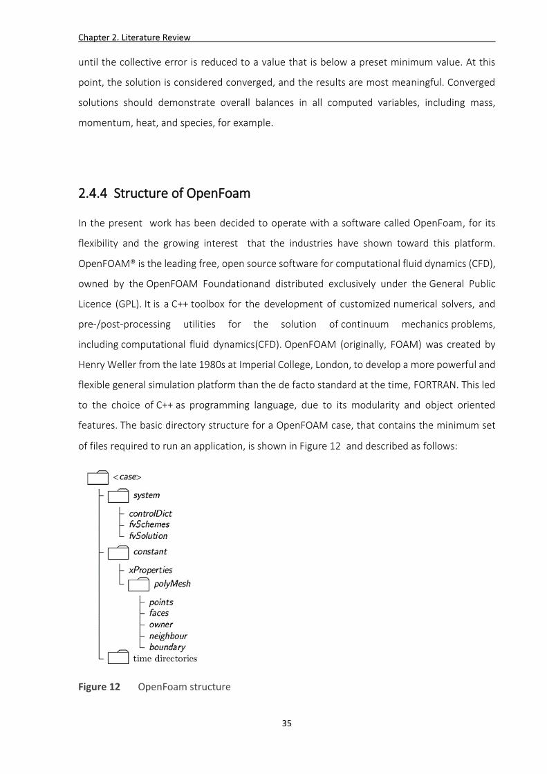
Chapter 2. Literature Review
35
until the collective error is reduced to a value that is below a preset minimum value. At this
point, the solution is considered converged, and the results are most meaningful. Converged
solutions should demonstrate overall balances in all computed variables, including mass,
momentum, heat, and species, for example.
2.4.4 Structure of OpenFoam
In the present work has been decided to operate with a software called OpenFoam, for its
flexibility and the growing interest that the industries have shown toward this platform.
OpenFOAM® is the leading free, open source software for computational fluid dynamics (CFD),
owned by the OpenFOAM Foundationand distributed exclusively under the General Public
Licence (GPL). It is a C++ toolbox for the development of customized numerical solvers, and
pre-/post-processing utilities for the solution of continuum mechanics problems,
including computational fluid dynamics(CFD). OpenFOAM (originally, FOAM) was created by
Henry Weller from the late 1980s at Imperial College, London, to develop a more powerful and
flexible general simulation platform than the de facto standard at the time, FORTRAN. This led
to the choice of C++ as programming language, due to its modularity and object oriented
features. The basic directory structure for a OpenFOAM case, that contains the minimum set
of files required to run an application, is shown in Figure 12 and described as follows:
Figure 12 OpenFoam structure
Chapter 2. Literature Review
36
A constant directory : that contains a full description of the case mesh in a
subdirectory polyMesh and files specifying physical properties for the application
concerned, e.g. transportProperties.
A system directory : for setting parameters associated with the solution procedure itself. It
contains at least the following 3 files: controlDict where run control parameters are set
including start/end time, time step and parameters for data output; fvSchemes where
discretisation schemes used in the solution may be selected at run-time; and, fvSolution where
the equation solvers, tolerances and other algorithm controls are set for the run.
The ‘time’ directories : containing individual files of data for particular fields. The data can be:
either, initial values and boundary conditions that the user must specify to define the problem;
or, results written to file by OpenFOAM. Note that the OpenFOAM fields must always be
initialised, even when the solution does not strictly require it, as in steady-state problems. The
name of each time directory is based on the simulated time at which the data is written. If the
simulations are initialized at time , the initial conditions are usually stored in a directory
named 0 or 0.000000e+00, depending on the name format specified.
37
Chapter 3
Materials & Methods
3.1 Introduction In the present thesis different software have been used in order to create the numerical
models, the geometry and the mesh and to post-process the numerical results. For this reason
in this chapter all the software settings are presented in detail. In the first part information on
the geometry and the grid independence are provided while in the second part details on
solver, turbulence model, initial conditions and the numerical schemes for the 2D and 3D model
are listed and explained.
3.2 Geometry and Mesh
In a numerical model the first step is building the geometry and the mesh. This is a crucial step
that will affect the results of the simulations and/or the convergence of the solution. The
present work is divided in two parts. In the first part a 2D Multi-phase model will be realized
and in the second part a 3D Single-phase model is discussed. The software used is Salome 7.5.1,
which is an open-source software that provides a generic platform for Pre- and Post-Processing
for numerical simulation. It is based on an open and flexible architecture made of reusable
components. Salome can be used for different aims :
Create/modify, import/export (IGES, STEP, BREP), repair/clean CAD models
Mesh CAD models, edit mesh, check mesh quality, import/export mesh (MED, UNV,
DAT, STL)
Handle physical properties and quantities attached to geometrical items
Perform computation using one or more external solvers (coupling)
Display computation results (scalar, vectorial)
Manage studies (create, save, reload)

Chapter 3. Material and Methods
38
3.2.1 2D Geometry
The 2D model is a simple pipe with baffles to reproduce the ideal structure of a static mixer.
Indeed the principle of a static mixer is to force the fluid to change direction improving the
mixing. The pipe is long 20 cm and has a diameter of 12.6 cm , with an internal channel for the
oil injection which has a diameter of 1.6mm. There are 4 baffles of 6.3 mm length and 2mm
wide, at same distance, in the central part of the pipe. The geometry is realized with Salome
7.5.1 with simple steps:
Create the points
Create the lines linking the points
Create a close contour (Wire)
Create the groups (inlet, outlet, wall)
The 2D geometry is shown in figure 13.
Figure 13 2D Geometry
After the geometry’s construction the next step is the mesh generation, using the same
software. The mesh is structured and the elements are triangles. Near the walls the grid is
refined to obtain better numerical results and the dimension of the single cell is chosen by
comparing to the minimum size necessary to capture the flow local effects. OpenFoam works
also in the 2D cases with 3D geometries where in the third dimension there is just one cell.
Therefore in order to not have problems during the process when exporting the Mesh from
Salome to OpenFoam, it will be realized a 2D mesh and then by using an extrusion the mesh
will become 3D. The figure 14 shows the 2D mesh.

Chapter 3. Material and Methods
39
(a)
(b)
Figure 14 2D Mesh (a) , (b)
For the 2D case, different grids have been created, with different refine grade but further
details will be given in the next section where the grid’s independence will be discussed.
3.2.2 3D Geometry
The 3D model is a cylindrical pipe, which contains 6 Kenics static mixer elements. The pipe has
the same length as for the 2D case 20 cm and has a diameter of 12.6 cm. Each static mixer
element has a length of 18.9 mm, so all together the module takes 113.4 mm, this is because
the ratio of L/D is equal to 1.5. The geometry is realized with Salome 7.5.1 in three main phases:
In the first phase a cylindrical pipe is realized by extrusion a disk of diameter 12.6mm.
In the second phase the static mixer element is drawn, starting with a rectangle. The
idea is to discretize the element using a finite number of rectangles which are rotated
around their axis from 0° to 180°. The helpful commands are “TRANSLATE” , “MIRROR”
and “ROTATION”. Then finally in order to obtain the static mixer shape , it is necessary
to link all the points of these rectangles together. Once the first element is ready, the

Chapter 3. Material and Methods
40
second one is realized using the function copy and then to obtain a solid by using the
“FUSION” function.
In the third phase is necessary cut the cylindrical pipe with the 6 static mixers to obtain
the final geometry and create all the groups which are fundamental to set the boundary
conditions once the geometry will be exported to OpenFoam.
The 6 Kenics static mixer and the cylindrical pipe which contain the static mixers are shown in
figures 15 and 16.
Figure 15 Section pipe + static mixer
Figure 16 Kenics static mixer
As for the 2D geometry, the mesh was realized using Salome, employing triangles for the 2D
faces and tetrahedrons for the 3D volumes. The total number of cells is 2,091,246 cells , which
is equivalent to 4 cells per millimetre. This number of cells allows a good accuracy of the results
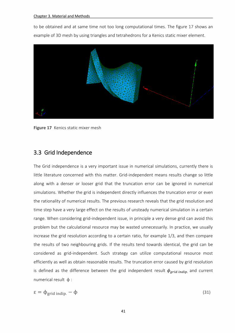
Chapter 3. Material and Methods
41
to be obtained and at same time not too long computational times. The figure 17 shows an
example of 3D mesh by using triangles and tetrahedrons for a Kenics static mixer element.
Figure 17 Kenics static mixer mesh
3.3 Grid Independence
The Grid independence is a very important issue in numerical simulations, currently there is
little literature concerned with this matter. Grid-independent means results change so little
along with a denser or looser grid that the truncation error can be ignored in numerical
simulations. Whether the grid is independent directly influences the truncation error or even
the rationality of numerical results. The previous research reveals that the grid resolution and
time step have a very large effect on the results of unsteady numerical simulation in a certain
range. When considering grid-independent issue, in principle a very dense grid can avoid this
problem but the calculational resource may be wasted unnecessarily. In practice, we usually
increase the grid resolution according to a certain ratio, for example 1/3, and then compare
the results of two neighbouring grids. If the results tend towards identical, the grid can be
considered as grid-independent. Such strategy can utilize computational resource most
efficiently as well as obtain reasonable results. The truncation error caused by grid resolution
is defined as the difference between the grid independent result 𝜙𝑔𝑟𝑖𝑑 𝑖𝑛𝑑𝑖𝑝. and current
numerical result ϕ :
ε = ϕgrid indip. − ϕ (31)
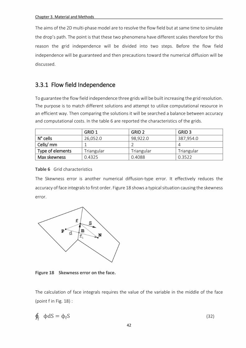
Chapter 3. Material and Methods
42
The aims of the 2D multi-phase model are to resolve the flow field but at same time to simulate
the drop’s path. The point is that these two phenomena have different scales therefore for this
reason the grid independence will be divided into two steps. Before the flow field
independence will be guaranteed and then precautions toward the numerical diffusion will be
discussed.
3.3.1 Flow field Independence
To guarantee the flow field independence three grids will be built increasing the grid resolution.
The purpose is to match different solutions and attempt to utilize computational resource in
an efficient way. Then comparing the solutions it will be searched a balance between accuracy
and computational costs. In the table 6 are reported the characteristics of the grids.
GRID 1 GRID 2 GRID 3
N° cells 26,052.0 98,922.0 387,954.0
Cells/ mm 1 2 4
Type of elements Triangular Triangular Triangular
Max skewness 0.4325 0.4088 0.3522
Table 6 Grid characteristics
The Skewness error is another numerical diffusion-type error. It effectively reduces the
accuracy of face integrals to first order. Figure 18 shows a typical situation causing the skewness
error.
Figure 18 Skewness error on the face.
The calculation of face integrals requires the value of the variable in the middle of the face
(point f in Fig. 18) :
∮ ϕdSf
= ϕfS (32)
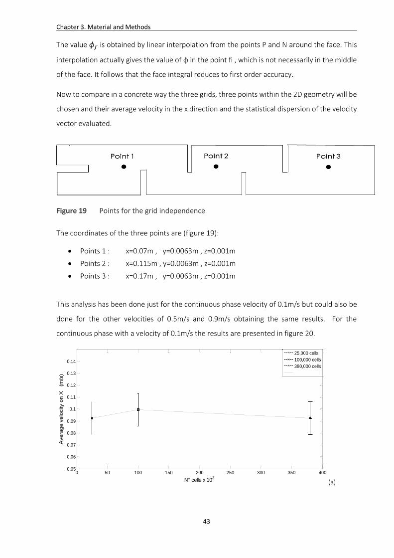
Chapter 3. Material and Methods
43
The value 𝜙𝑓 is obtained by linear interpolation from the points P and N around the face. This
interpolation actually gives the value of φ in the point fi , which is not necessarily in the middle
of the face. It follows that the face integral reduces to first order accuracy.
Now to compare in a concrete way the three grids, three points within the 2D geometry will be
chosen and their average velocity in the x direction and the statistical dispersion of the velocity
vector evaluated.
Figure 19 Points for the grid independence
The coordinates of the three points are (figure 19):
Points 1 : x=0.07m , y=0.0063m , z=0.001m
Points 2 : x=0.115m , y=0.0063m , z=0.001m
Points 3 : x=0.17m , y=0.0063m , z=0.001m
This analysis has been done just for the continuous phase velocity of 0.1m/s but could also be
done for the other velocities of 0.5m/s and 0.9m/s obtaining the same results. For the
continuous phase with a velocity of 0.1m/s the results are presented in figure 20.
(a)
0 50 100 150 200 250 300 350 4000.05
0.06
0.07
0.08
0.09
0.1
0.11
0.12
0.13
0.14
N° celle x 103
Avera
ge v
elo
city o
n X
(
m/s
)
25,000 cells
100,000 cells
380,000 cells
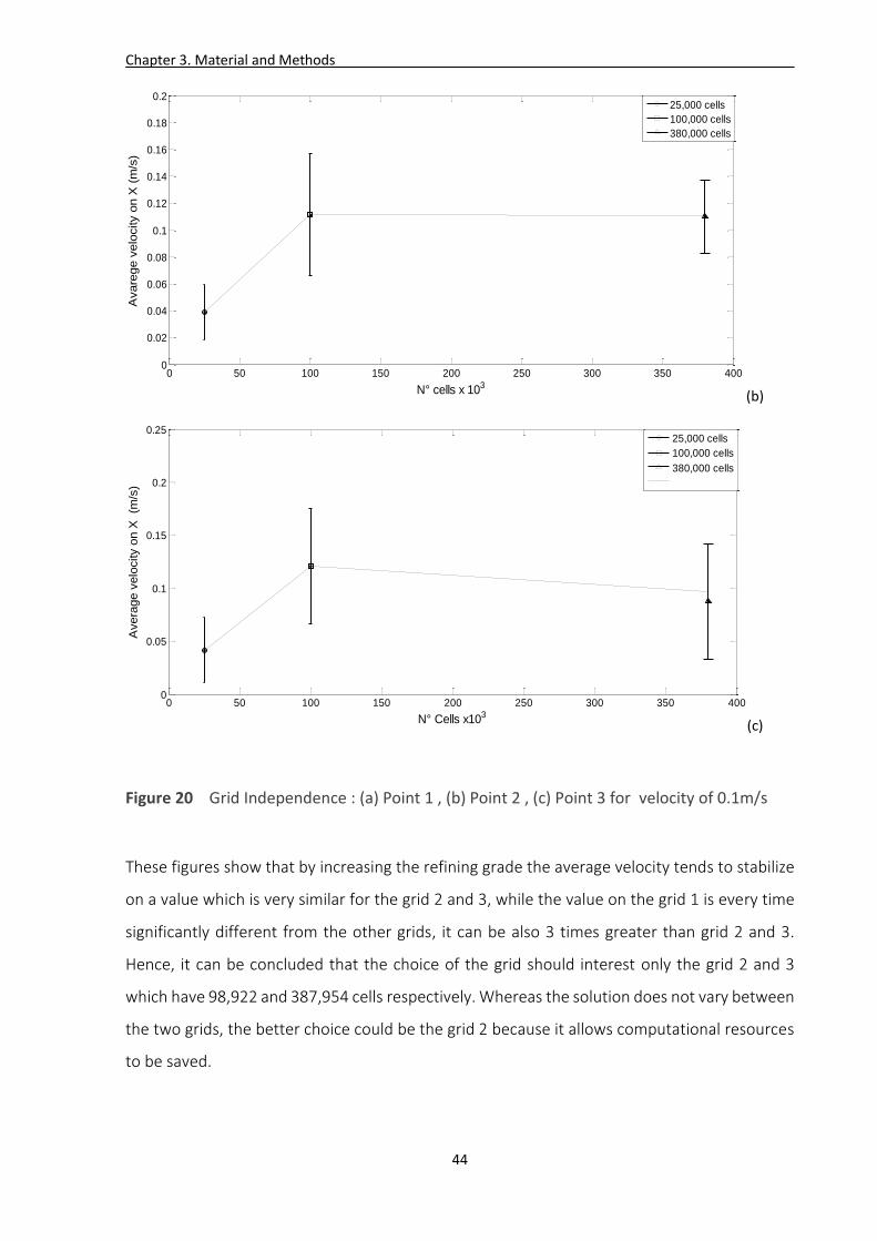
Chapter 3. Material and Methods
44
(b)
(c)
Figure 20 Grid Independence : (a) Point 1 , (b) Point 2 , (c) Point 3 for velocity of 0.1m/s
These figures show that by increasing the refining grade the average velocity tends to stabilize
on a value which is very similar for the grid 2 and 3, while the value on the grid 1 is every time
significantly different from the other grids, it can be also 3 times greater than grid 2 and 3.
Hence, it can be concluded that the choice of the grid should interest only the grid 2 and 3
which have 98,922 and 387,954 cells respectively. Whereas the solution does not vary between
the two grids, the better choice could be the grid 2 because it allows computational resources
to be saved.
0 50 100 150 200 250 300 350 4000
0.02
0.04
0.06
0.08
0.1
0.12
0.14
0.16
0.18
0.2
N° cells x 103
Avare
ge v
elo
city o
n X
(m
/s)
25,000 cells
100,000 cells
380,000 cells
0 50 100 150 200 250 300 350 4000
0.05
0.1
0.15
0.2
0.25
N° Cells x103
Avera
ge v
elo
city o
n X
(m
/s)
25,000 cells
100,000 cells
380,000 cells
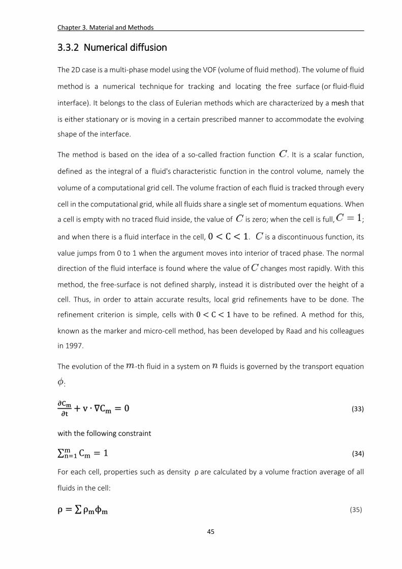
Chapter 3. Material and Methods
45
3.3.2 Numerical diffusion
The 2D case is a multi-phase model using the VOF (volume of fluid method). The volume of fluid
method is a numerical technique for tracking and locating the free surface (or fluid-fluid
interface). It belongs to the class of Eulerian methods which are characterized by a mesh that
is either stationary or is moving in a certain prescribed manner to accommodate the evolving
shape of the interface.
The method is based on the idea of a so-called fraction function . It is a scalar function,
defined as the integral of a fluid's characteristic function in the control volume, namely the
volume of a computational grid cell. The volume fraction of each fluid is tracked through every
cell in the computational grid, while all fluids share a single set of momentum equations. When
a cell is empty with no traced fluid inside, the value of is zero; when the cell is full, ;
and when there is a fluid interface in the cell, 0 < C < 1. is a discontinuous function, its
value jumps from 0 to 1 when the argument moves into interior of traced phase. The normal
direction of the fluid interface is found where the value of changes most rapidly. With this
method, the free-surface is not defined sharply, instead it is distributed over the height of a
cell. Thus, in order to attain accurate results, local grid refinements have to be done. The
refinement criterion is simple, cells with 0 < C < 1 have to be refined. A method for this,
known as the marker and micro-cell method, has been developed by Raad and his colleagues
in 1997.
The evolution of the -th fluid in a system on fluids is governed by the transport equation
:
∂Cm
∂t+ v ∙ ∇Cm = 0 (33)
with the following constraint
∑ Cm = 1mn=1 (34)
For each cell, properties such as density ρ are calculated by a volume fraction average of all
fluids in the cell:
ρ = ∑ ρmϕm (35)
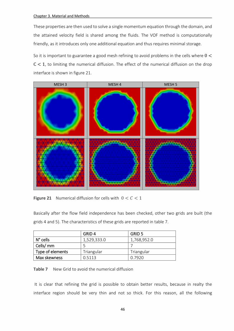
Chapter 3. Material and Methods
46
These properties are then used to solve a single momentum equation through the domain, and
the attained velocity field is shared among the fluids. The VOF method is computationally
friendly, as it introduces only one additional equation and thus requires minimal storage.
So it is important to guarantee a good mesh refining to avoid problems in the cells where 0 <
C < 1, to limiting the numerical diffusion. The effect of the numerical diffusion on the drop
interface is shown in figure 21.
MESH 3 MESH 4 MESH 5
Figure 21 Numerical diffusion for cells with 0 < 𝐶 < 1
Basically after the flow field independence has been checked, other two grids are built (the
grids 4 and 5). The characteristics of these grids are reported in table 7.
GRID 4 GRID 5
N° cells 1,529,333.0 1,768,952.0
Cells/ mm 5 7
Type of elements Triangular Triangular
Max skewness 0.5113 0.7920
Table 7 New Grid to avoid the numerical diffusion
It is clear that refining the grid is possible to obtain better results, because in realty the
interface region should be very thin and not so thick. For this reason, all the following

Chapter 3. Material and Methods
47
calculations have been obtained using the finest grid, namely grid 5, in order to capture all the
local flow effects.
3.4 Settings 2D Multi-phase Model
In this paragraph, all the settings necessary for the simulations will be listed and explained, to
understand the reasons of each choice. It will be clarified which physical parameters have been
used as input into the numerical model and what boundary conditions were set.
3.4.1 Choice of the Solver
The solver for the 2D multi-phase model has been chosen into the OpenFoam platform
between several solvers available (it is reported the link to the web site
http://www.openfoam.org/features/standard-solvers.php ). According to the characteristics
of these simulations the more suitable solver has been “InterFoam” , which belongs to the
Multiphase section and it is a Solver for 2 incompressible, isothermal immiscible fluids using a
VOF (volume of fluid) phase-fraction based interface capturing approach. Indeed the aim of this
work is to study a single oil drop to further understand the mixing processes. To easily reach
the stationary time a modified version of this solver was performed “LTSInterFOAM”, which is
a local time stepping (LTS, steady-state) solver for 2 incompressible, isothermal immiscible
fluids using a VOF (volume of fluid) phase-fraction based interface capturing approach.
3.4.2 Choice of the turbulence Model
The simulations have been performed with a Reynolds number ranging from 3,000 to more
than 10,000 so a turbulence model is necessary. OpenFOAM offers a large range of methods
and models to simulate turbulence as :
Reynolds-average simulation (RAS), also known as Reynolds-averaged Navier-Stokes
(RANS).
Large eddy simulation (LES)
Direct Numerical Simulation (DNS)
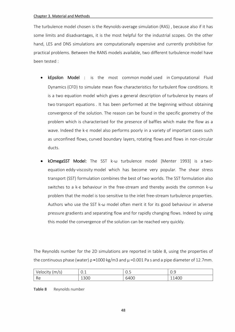
Chapter 3. Material and Methods
48
The turbulence model chosen is the Reynolds-average simulation (RAS) , because also if it has
some limits and disadvantages, it is the most helpful for the industrial scopes. On the other
hand, LES and DNS simulations are computationally expensive and currently prohibitive for
practical problems. Between the RANS models available, two different turbulence model have
been tested :
kEpsilon Model : is the most common model used in Computational Fluid
Dynamics (CFD) to simulate mean flow characteristics for turbulent flow conditions. It
is a two equation model which gives a general description of turbulence by means of
two transport equations . It has been performed at the beginning without obtaining
convergence of the solution. The reason can be found in the specific geometry of the
problem which is characterised for the presence of baffles which make the flow as a
wave. Indeed the k-ε model also performs poorly in a variety of important cases such
as unconfined flows, curved boundary layers, rotating flows and flows in non-circular
ducts.
kOmegaSST Model: The SST k-ω turbulence model [Menter 1993] is a two-
equation eddy-viscosity model which has become very popular. The shear stress
transport (SST) formulation combines the best of two worlds. The SST formulation also
switches to a k-ε behaviour in the free-stream and thereby avoids the common k-ω
problem that the model is too sensitive to the inlet free-stream turbulence properties.
Authors who use the SST k-ω model often merit it for its good behaviour in adverse
pressure gradients and separating flow and for rapidly changing flows. Indeed by using
this model the convergence of the solution can be reached very quickly.
The Reynolds number for the 2D simulations are reported in table 8, using the properties of
the continuous phase (water) ρ =1000 kg/m3 and µ =0.001 Pa s and a pipe diameter of 12.7mm.
Velocity (m/s) 0.1 0.5 0.9
Re 1300 6400 11400
Table 8 Reynolds number
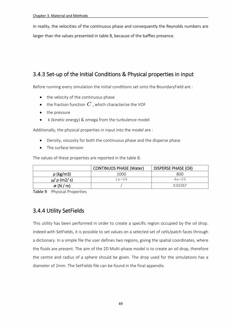
Chapter 3. Material and Methods
49
In reality, the velocities of the continuous phase and consequently the Reynolds numbers are
larger than the values presented in table 8, because of the baffles presence.
3.4.3 Set-up of the Initial Conditions & Physical properties in input
Before running every simulation the initial conditions set onto the BoundaryField are :
the velocity of the continuous phase
the fraction function , which characterize the VOF
the pressure
k (kinetic energy) & omega from the turbulence model
Additionally, the physical properties in input into the model are :
Density, viscosity for both the continuous phase and the disperse phase
The surface tension
The values of these properties are reported in the table 8.
CONTINUOS PHASE (Water) DISPERSE PHASE (Oil)
ρ (kg/m3) 1000 800
µ/ ρ (m2/ s) 1e-06 4e-06
𝝈 (N / m) / 0.02267
Table 9 Physical Properties
3.4.4 Utility SetFields
This utility has been performed in order to create a specific region occupied by the oil drop.
Indeed with SetFields, it is possible to set values on a selected set of cells/patch faces through
a dictionary. In a simple file the user defines two regions, giving the spatial coordinates, where
the fluids are present. The aim of the 2D Multi-phase model is to create an oil drop, therefore
the centre and radius of a sphere should be given. The drop used for the simulations has a
diameter of 2mm. The SetFields file can be found in the final appendix.

Chapter 3. Material and Methods
50
3.5 Settings 3D Single-phase Model
The aim of the 3D single-phase model is to produce a real flow field when the continuous phase
which is water is mixed in a pipe with 6 Kenics static mixer. Basically, information on the velocity
field and the shear stress field are desired to assess how much changes in velocity of the
continuous phase affects the mixing performance.
3.5.1 Choice of the Solver
The solver “pisoFoam” has been used for this single-phase model because it is a transient solver
for incompressible flow. Additionally, if in this case the geometry is much more complex
compared to the 2D case, the solver needs less computational resources.
3.5.2 Choice of the turbulence Model
In the 3D case has been performed the same turbulence model used for the 2D simulation,
namely the k-Omega SST model.
The Reynolds numbers for the 3D simulations are reported in table 9. To compute the Reynolds
numbers the properties of the water ρ =1000 kg/m3 and µ =0.001 Pas and a pipe diameter of
12.7mm are used. The velocity used for the calculations takes account the space occupied by
the static mixer, which reduces the section available for the flow.
Superficial velocity (m/s) 0.1 0.5 0.9
Velocity (m/s) /vacuum degree 0.16 0.76 1.4
Re 2200 9700 17700
Chapter 3. Material and Methods
51
3.5.3 Set-up of the Initial Conditions & Physical properties in input
As for the 2D model, before to run every simulation the initial conditions set onto the
BoundaryField are :
the velocity of the continuous phase
the pressure
k (kinetic energy) & omega from the turbulence model. To help the convergence of
the solution an appropriate initialization of the turbulence parameters k and Ω has
been done by using formula taken from the literature review.
Furthermore, the only physical property as an input is the viscosity of the continuous phase
(water).
3.6 Cluster BlueBear
The Birmingham Environment for Academic Research (BEAR) is a collection of complimentary
IT resources managed by IT Services that are designed to help research, all of which are free at
the point of use. The procurement for the current suite of services resulted in a framework
agreement with OCF, IBM, Adaptive Computing, Mechdyne and IOCOM who bring different
areas of expertise to the overall research environment. One of the components of BEAR is
BlueBEAR, a Linux-based batch processing High Performance Computing (HPC) cluster. The
additional modelling power will enable researchers to process larger, more detailed, more
accurate simulations and test cases in less time than was possible on the previous service.
Within the School of Chemistry Professor Roy Johnston and his team, one of the service’s major
users, are using the Linux HPC service for research into many areas including computational
nanoscience. Professor Johnson’s team is trying to understand how to create more cost
effective and more environmentally friendly catalysts for fuel cells and hydrogen cars, for
example.
The centrally-funded BlueBEAR cluster is based on IBM's iDataPlex servers and consists of:
dual-processor 8-core (16 cores/node) 64-bit 2.2 GHz Intel Sandy Bridge E5-2660 login
nodes with 64 GB of memory logon nodes in a round-robin configuration for resiliency
Chapter 3. Material and Methods
52
1 dual-processor 8-core (16 cores/node) 64-bit 2.2 GHz Intel Sandy Bridge E5-2660 login
node with 64 GB of memory for applications that make use of a Graphical user Interface
(GUI)
72 dual-processor 8-core (16 cores/node) 64-bit 2.2 GHz Intel Sandy Bridge E5-2660
worker nodes with 32 GB of memory giving a total of 1152 cores
dual-processor 8-core (16 cores/node) 64-bit 2.2 GHz Intel Sandy Bridge E5-2660
worker nodes with 256 GB of memory forming a large memory (SMP) service
2 GPU-assisted compute nodes with 2 two 8 core 64-bit 2.2 GHz Intel Sandy Bridge E5-
2660 processors, 32 GB of memory and an nVIDIA Kepler-based Tesla K20 GPU forming
a GPGPU service
over 150 TB (raw) disk space primarily allocated to BlueBEAR users using IBM's GPFS
cluster file system
The theoretical peak performance of the centrally-funded compute nodes is 1216 (cores) * 2.2
(GHz) * 8 (floating point operations/cycle) = 21.4 TFlop/s.
Thanks to this powerful cluster, it has been possible to easily run complex simulations with grids
really fine. To do this it has been necessary to learn how to handle the cluster interface. The
main steps needed to run a simulation are reported below:
Register to the BluBEAR cluster and create an user folder
Transfer the data for the simulation (solver, turbulence model, geometry) into the user
folder
Add into the simulation settings a file that decomposes the computational domain in
function of the number of cores used
Create and run a script where the user defined all the commands necessary to perform
the simulation
Transfer to your own laptop the numerical results
To conclude a job submitted for BluBEAR is attached in the final appendix.

53
Chapter 4
Results
4.1 Introduction
In this chapter the post- processing of the numerical solution of the simulations by using Matlab
will be discussed. In the first part of this section the results from the 2D Multi-phase model will
be presented and a study of the drop surface in order to observe the changes of two important
properties such as the shear stress and the energy turbulence dissipation will be done. After
this, a streamlines analysis will be shown, to link the break up phenomenon with the local flow
characteristics. In the second part of this section the results from the 3D Single-phase model
will be also presented, by using an image flow characterization.
4.2 2D Multi-phase Results
The 2D Multi-phase simulations have been performed changing the continuous phase (water)
velocity, to investigate the effect on the mixing performance, attempting to observe changes
for the droplet break up. The same geometry has been run for three times with different values
of the velocity: 0.1m/s , 0.5m/s and 0.9m/s with the aim to discover why the experimental data
from a previous work (Forte Giuseppe (2015)) have shown a better mixing performance around
0.5m/s and not 0.9m/s, which is the highest velocity. Consequently, two ideas have been
developed during post-processing:
Comparing the local analysis on the oil drop surface with a global analysis
A streamlines analysis

Chapter 4. Results
54
Before to present in details the post- processing analysis, the flow field for the continuous
phase velocity of 0.1m/s is reported in figure 22. For the velocities of 0.5m/s and 0.9m/s similar
considerations can be done, so their flow fields are not presented.
Figure 22 Flow field for 0.1m/s
The magnitude of the velocity is presented in figure 22. It is very similar to the X-velocity
because in this system the Y-velocity is a small component. The flow field shows that there are
two regions:
The inlet for the water, where the flow is uniform and the velocity value of about
0.1m/s is reached
The region which contains the baffles, where there are recirculation areas behind the
baffles and regions at high velocity near the centre of the pipe

Chapter 4. Results
55
4.2.1 Analysis of the oil drop surface
The drop break up is a local phenomenon which rises from the balance between an external
disturbing force, induced by the flow field, which tries to deform the droplet and an internal
restoring force which tries to keep the droplet in its original shape. The developed idea is to
observe and study the drop surface and in particular take account of changes of two important
parameters:
The shear stress
The energy turbulence dissipation
This is because both the parameters can be linked with the external disturbing force causing
the drop break up. It is also possible to follow the shape changes of the drop and study the
deformation in the x and y directions.
Basically, in order to study the drop surface, it is necessary to import the raw data of the
simulations from OpenFoam to Matlab in a matrix form. The imported matrix contains all the
numerical variables defined in each cell of the numerical grid. So to re-build the drop surface
and keep only the variables defined onto it, a Matlab script has been created (which is attached
in the final appendix). This code, by using the value of the mass fraction, is able to find the cells
where the C function or mass fraction has values between 0 and 1, namely it finds the interface
cells. An example of drop re-built with Matlab compared with a drop image took from the
OpenFoam viewer is shown in figure 22.
(a)

Chapter 4. Results
56
(b)
Figure 23 Drop re-built with Matlab (a) , Drop image from simulation (b)
In all the points which make up the drop contour, it is known the velocity in x ,y directions , the
shear stress , the energy dissipation and other variables, so a complete analysis can be done. In
order to explain how the Matlab script works to convert the initial matrix in a new matrix a
simple scheme is presented in figure 23.
Figure 24 Steps of the Matlab Script
In the next step the number of droplets to analyse it has been decided. In each simulation,
which lasts for two seconds, and for different continuous phase velocities, the time at which
the first droplet breakage occurs was obtained. The break up time was then divided in three
equal intervals, to focus the analysis only on 4 drops. This time division is done because by
increasing the velocity of the continuous phase in theory the time when the first rupture
happens is expected to decrease, so with an equal division it is possible to then compare drops
at different velocities. All the drops observed at different time and different continuous phase
velocities are reported in table 10 with the Matlab reconstructions.
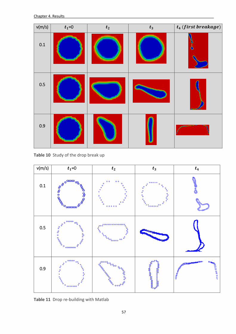
Chapter 4. Results
57
v(m/s) 𝒕𝟏=0 𝒕𝟐 𝒕𝟑 𝒕𝟒 (𝒇𝒊𝒓𝒔𝒕 𝒃𝒓𝒆𝒂𝒌𝒂𝒈𝒆)
0.1
0.5
0.9
Table 10 Study of the drop break up
v(m/s) 𝒕𝟏=0 𝒕𝟐 𝒕𝟑 𝒕𝟒
0.1
0.5
0.9
Table 11 Drop re-building with Matlab
0.145 0.15 0.155 0.16 0.165
2
4
6
8
10
12
14x 10
-3
X(m)
Y(m
)
bubble shape
0.0890.08920.08940.08960.08980.090.09020.09049
9.2
9.4
9.6
9.8
10
10.2
x 10-3
X(m)
Y(m)
bubble shape
0.121 0.1212 0.1214 0.1216 0.1218 0.122 0.1222 0.1224 0.1226 0.1228
8.8
9
9.2
9.4
9.6
9.8
10
10.2
10.4
10.6x 10
-3
X(m)
Y(m
)
bubble shape
0.134 0.136 0.138 0.14 0.142 0.144 0.146 0.148 0.15 0.152 0.1540
0.002
0.004
0.006
0.008
0.01
0.012
0.014
X(m)
Y(m
)
bubble shape
0.0485 0.049 0.0495 0.05 0.0505 0.051 0.05155
5.5
6
6.5
7
7.5x 10
-3
X(m)
Y(m
)
bubble shape
0.104 0.1045 0.105 0.1055 0.106 0.1065 0.107 0.10752
2.5
3
3.5
4
x 10-3
X(m)
Y(m
)
bubble shape
0.049 0.0495 0.05 0.0505 0.051 0.05155.4
5.6
5.8
6
6.2
6.4
6.6
6.8
7
7.2
7.4x 10
-3
X(m)
Y(m
)
bubble shape
0.175 0.18 0.185 0.19 0.195 0.20
0.002
0.004
0.006
0.008
0.01
0.012
0.014
X(m)
Y(m
)
bubble shape
0.16 0.165 0.17 0.175 0.18 0.185 0.19 0.1954
5
6
7
8
9
10
11
12
13x 10
-3
X(m)
Y(m
)
bubble shape
0.1436 0.1438 0.144 0.1442 0.1444 0.1446 0.1448
4.5
5
5.5
6
6.5
7
7.5
8
8.5x 10
-3
X(m)
Y(m
)
bubble shape
0.0968 0.097 0.0972 0.0974 0.0976 0.0978 0.098 0.0982 0.0984 0.0986
5.5
6
6.5
7
7.5x 10
-3
X(m)
Y(m
)
bubble shape
0.049 0.0495 0.05 0.0505 0.051 0.05155.4
5.6
5.8
6
6.2
6.4
6.6
6.8
7
7.2
7.4x 10
-3
X(m)
Y(m
)
bubble shape
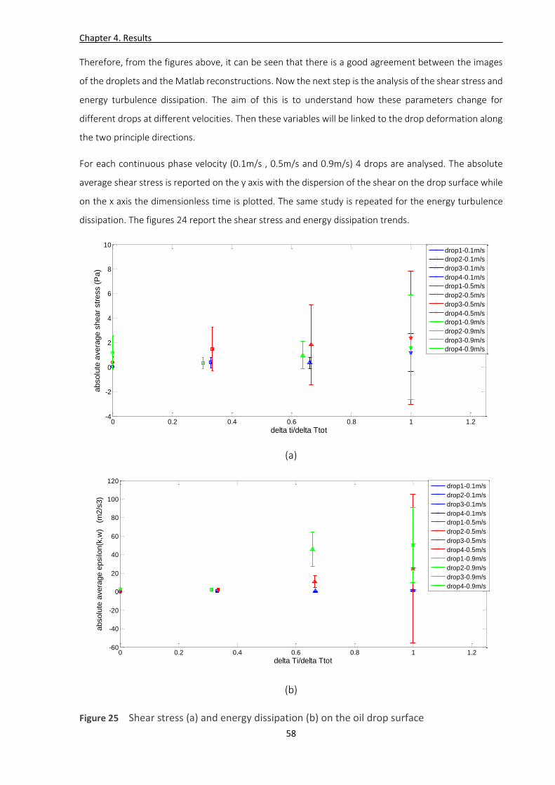
Chapter 4. Results
58
Therefore, from the figures above, it can be seen that there is a good agreement between the images
of the droplets and the Matlab reconstructions. Now the next step is the analysis of the shear stress and
energy turbulence dissipation. The aim of this is to understand how these parameters change for
different drops at different velocities. Then these variables will be linked to the drop deformation along
the two principle directions.
For each continuous phase velocity (0.1m/s , 0.5m/s and 0.9m/s) 4 drops are analysed. The absolute
average shear stress is reported on the y axis with the dispersion of the shear on the drop surface while
on the x axis the dimensionless time is plotted. The same study is repeated for the energy turbulence
dissipation. The figures 24 report the shear stress and energy dissipation trends.
(a)
(b)
Figure 25 Shear stress (a) and energy dissipation (b) on the oil drop surface
0 0.2 0.4 0.6 0.8 1 1.2-4
-2
0
2
4
6
8
10
delta ti/delta Ttot
absolu
te a
vera
ge s
hear
str
ess (
Pa)
drop1-0.1m/s
drop2-0.1m/s
drop3-0.1m/s
drop4-0.1m/s
drop1-0.5m/s
drop2-0.5m/s
drop3-0.5m/s
drop4-0.5m/s
drop1-0.9m/s
drop2-0.9m/s
drop3-0.9m/s
drop4-0.9m/s
0 0.2 0.4 0.6 0.8 1 1.2-60
-40
-20
0
20
40
60
80
100
120
delta Ti/delta Ttot
absolu
te a
vera
ge e
psilo
n(k
,w)
(m
2/s
3)
drop1-0.1m/s
drop2-0.1m/s
drop3-0.1m/s
drop4-0.1m/s
drop1-0.5m/s
drop2-0.5m/s
drop3-0.5m/s
drop4-0.5m/s
drop1-0.9m/s
drop2-0.9m/s
drop3-0.9m/s
drop4-0.9m/s
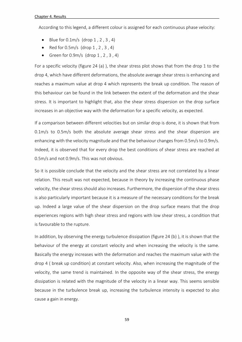
Chapter 4. Results
59
According to this legend, a different colour is assigned for each continuous phase velocity:
Blue for 0.1m/s (drop 1 , 2 , 3 , 4)
Red for 0.5m/s (drop 1 , 2 , 3 , 4)
Green for 0.9m/s (drop 1 , 2 , 3 , 4)
For a specific velocity (figure 24 (a) ), the shear stress plot shows that from the drop 1 to the
drop 4, which have different deformations, the absolute average shear stress is enhancing and
reaches a maximum value at drop 4 which represents the break up condition. The reason of
this behaviour can be found in the link between the extent of the deformation and the shear
stress. It is important to highlight that, also the shear stress dispersion on the drop surface
increases in an objective way with the deformation for a specific velocity, as expected.
If a comparison between different velocities but on similar drop is done, it is shown that from
0.1m/s to 0.5m/s both the absolute average shear stress and the shear dispersion are
enhancing with the velocity magnitude and that the behaviour changes from 0.5m/s to 0.9m/s.
Indeed, it is observed that for every drop the best conditions of shear stress are reached at
0.5m/s and not 0.9m/s. This was not obvious.
So it is possible conclude that the velocity and the shear stress are not correlated by a linear
relation. This result was not expected, because in theory by increasing the continuous phase
velocity, the shear stress should also increases. Furthermore, the dispersion of the shear stress
is also particularly important because it is a measure of the necessary conditions for the break
up. Indeed a large value of the shear dispersion on the drop surface means that the drop
experiences regions with high shear stress and regions with low shear stress, a condition that
is favourable to the rupture.
In addition, by observing the energy turbulence dissipation (figure 24 (b) ), it is shown that the
behaviour of the energy at constant velocity and when increasing the velocity is the same.
Basically the energy increases with the deformation and reaches the maximum value with the
drop 4 ( break up condition) at constant velocity. Also, when increasing the magnitude of the
velocity, the same trend is maintained. In the opposite way of the shear stress, the energy
dissipation is related with the magnitude of the velocity in a linear way. This seems sensible
because in the turbulence break up, increasing the turbulence intensity is expected to also
cause a gain in energy.
Chapter 4. Results
60
To link both the shear stress and the energy dissipation trends to the deformation of the drops,
a study to value the deformation on x and y directions is done, by using the dispersion of the x
and y drop coordinates. In the figure below an extent of the drop deformation is given for all
the drops, for different velocities.
(a)
(b)
Figure 26 Link between shear stress , energy dissipation and deformation
As for the plots above, a different colour is assigned for each continuous phase velocity,
according to this legend:
Blue for 0.1m/s (drop 1 , 2 , 3 , 4)
0.2 0.3 0.4 0.5 0.6 0.7 0.8 0.9 10
0.5
1
1.5
2
2.5
3
position X/L
shear
str
ess a
bs m
ean(P
a)
0.2 0.3 0.4 0.5 0.6 0.7 0.8 0.9 1-10
0
10
20
30
40
50
60
position X/L
Absolu
te a
vera
ge e
psilo
n (
m2/s
3)
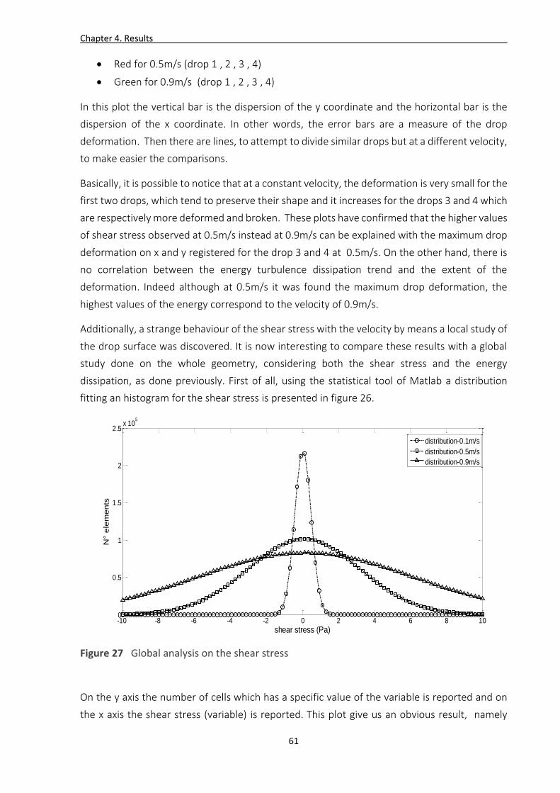
Chapter 4. Results
61
Red for 0.5m/s (drop 1 , 2 , 3 , 4)
Green for 0.9m/s (drop 1 , 2 , 3 , 4)
In this plot the vertical bar is the dispersion of the y coordinate and the horizontal bar is the
dispersion of the x coordinate. In other words, the error bars are a measure of the drop
deformation. Then there are lines, to attempt to divide similar drops but at a different velocity,
to make easier the comparisons.
Basically, it is possible to notice that at a constant velocity, the deformation is very small for the
first two drops, which tend to preserve their shape and it increases for the drops 3 and 4 which
are respectively more deformed and broken. These plots have confirmed that the higher values
of shear stress observed at 0.5m/s instead at 0.9m/s can be explained with the maximum drop
deformation on x and y registered for the drop 3 and 4 at 0.5m/s. On the other hand, there is
no correlation between the energy turbulence dissipation trend and the extent of the
deformation. Indeed although at 0.5m/s it was found the maximum drop deformation, the
highest values of the energy correspond to the velocity of 0.9m/s.
Additionally, a strange behaviour of the shear stress with the velocity by means a local study of
the drop surface was discovered. It is now interesting to compare these results with a global
study done on the whole geometry, considering both the shear stress and the energy
dissipation, as done previously. First of all, using the statistical tool of Matlab a distribution
fitting an histogram for the shear stress is presented in figure 26.
Figure 27 Global analysis on the shear stress
On the y axis the number of cells which has a specific value of the variable is reported and on
the x axis the shear stress (variable) is reported. This plot give us an obvious result, namely
-10 -8 -6 -4 -2 0 2 4 6 8 100
0.5
1
1.5
2
2.5x 10
5
shear stress (Pa)
N° e
lem
ents
distribution-0.1m/s
distribution-0.5m/s
distribution-0.9m/s

Chapter 4. Results
62
increasing the continuous phase velocity the N° of cells which has an higher value of shear
stress increase or in other words increasing the velocity the variance of these curve increases.
This behaviour of the shear stress is different from the behaviour highlighted with the local
analysis of the drop surface.
Hence to clarify this discrepancy, the shear stress on the drop surface for each drop will be
compared with the global shear stress just presented, changing the continuous phase velocity.
The same analysis will be done also for the energy dissipation.
(a)
(b)
Figure 28 Local approach vs Global approach
0.1 0.2 0.3 0.4 0.5 0.6 0.7 0.8 0.9 10
0.5
1
1.5
2
2.5
3
velocity (m/s)
Absolu
te a
vera
ge s
hear
str
ess (
Pa)
Global statistic shear
shear-surface drop1
shear-surface drop2
shear-surface drop3
shear-surface drop4
0.1 0.2 0.3 0.4 0.5 0.6 0.7 0.8 0.9 10
10
20
30
40
50
60
velocity (m/s)
Absolu
te a
vera
ge e
nerg
y d
issip
ation (
m2/s
3)
GLOBAL ENERGY-DISSIPATION
ENERGY-surface drop1
ENERGY-surface drop2
ENERGY-surface drop3
ENERGY-surface drop4

Chapter 4. Results
63
Figure 27 (a) reports the average shear stress on y axis and different continuous phase velocity
on the x axis. The black line is the global shear stress, namely it is another way to represent the
previous distributions, while the other lines feature the absolute average shear stress evaluated
on the drop surface for each drop, at different velocity.
Two important aspects should be noticed :
The global and the local shear stress trend are different. The first one takes into account
the whole fluid flow field and the other it is focused on the drop surface where changes
of the shape take place. It is also shown how for all the drops, except the drop 1 , the
absolute average shear stress decreases from 0.5m/s to 0.9m/s.
Only the drop 1 , drop initialized at time t=0, does not follow the local trend but follow
the global trend. This can be explained as a numerical effect of the initialization process.
On the other hand, the figure 27 (b) shows an agreement between the local approach and the
global approach because in both the cases the energy grows with the velocity. The energy
turbulence dissipation is a function of the turbulence intensity so it is no surprise that its
module enhance increasing the continuous phase velocity.
4.2.2 Streamlines analysis
For a better understanding of the previous shear stress trend, a streamlines analysis has been
performed to attempt to link the position of the drops with the velocity of the continuous
phase. The streamlines utility is an OpenFoam filter which is available for the user during the
post-processing of the solution with Paraview. This filter allows the creation of several
streamlines with a specific length and with a specific distance from the centre of the pipe cross
section. The user specifies also the number of points necessary to build the streamline, called
“seed points”. In the figure below, the streamlines for the 2D geometry are shown. In figure 28
the streamline colour changes with the module of the velocity.
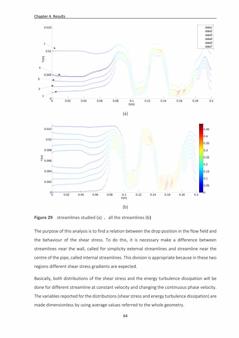
Chapter 4. Results
64
(a)
(b)
Figure 29 streamlines studied (a) , all the streamlines (b)
The purpose of this analysis is to find a relation between the drop position in the flow field and
the behaviour of the shear stress. To do this, it is necessary make a difference between
streamlines near the wall, called for simplicity external streamlines and streamline near the
centre of the pipe, called internal streamlines. This division is appropriate because in these two
regions different shear stress gradients are expected.
Basically, both distributions of the shear stress and the energy turbulence dissipation will be
done for different streamline at constant velocity and changing the continuous phase velocity.
The variables reported for the distributions (shear stress and energy turbulence dissipation) are
made dimensionless by using average values referred to the whole geometry.
0 0.02 0.04 0.06 0.08 0.1 0.12 0.14 0.16 0.18 0.20
0.005
0.01
0.015
X(m)
Y(m
)
data1
data2
data3
data4
data5
data7
1
2
3
4
7
0 0.02 0.04 0.06 0.08 0.1 0.12 0.14 0.16 0.18 0.20
0.002
0.004
0.006
0.008
0.01
0.012
X(m)
Y(m
)
0
0.05
0.1
0.15
0.2
0.25
0.3
0.35
0.4
0.45

Chapter 4. Results
65
(a)
(b)
Figure 30 Distributions of shear stress (a) and energy turbulence dissipation (b)
The charts reported consider 7 streamlines for a constant velocity of 0.1 m/s. The charts for the
same streamlines but for the other velocities (0.5m/s and 0.9m/s) have given the same trends
hence they are not presented.
The figure 29 (a) and (b) shows that moving from the external streamlines (stream 1) to the
internal streamlines ( stream 4 or 7) the distributions of shear stress and energy turbulence
dissipation are moving to the left, toward smaller values of the variables. From another point
of view, this means that on the internal streamlines, the variations of the properties tend to be
smaller compare with the external streamlines. To clarify this behaviour, the same streamlines
10-4
10-3
10-2
10-1
100
101
102
0
20
40
60
80
100
120
energy dissipation / average energy dissipation
N°
data2
stream1-0.1m/s
stream2-0.1m/s
stream3-0.1m/s
stream4-0.1m/s
stream7-0.1m/s
10-6
10-5
10-4
10-3
10-2
10-1
100
101
102
0
20
40
60
80
100
120
shear stress / average shear stress
N°
data1
stream1-0.1m/s
stream2-0.1m/s
stream3-0.1m/s
stream4-0.1m/s
stream7-0.1m/s
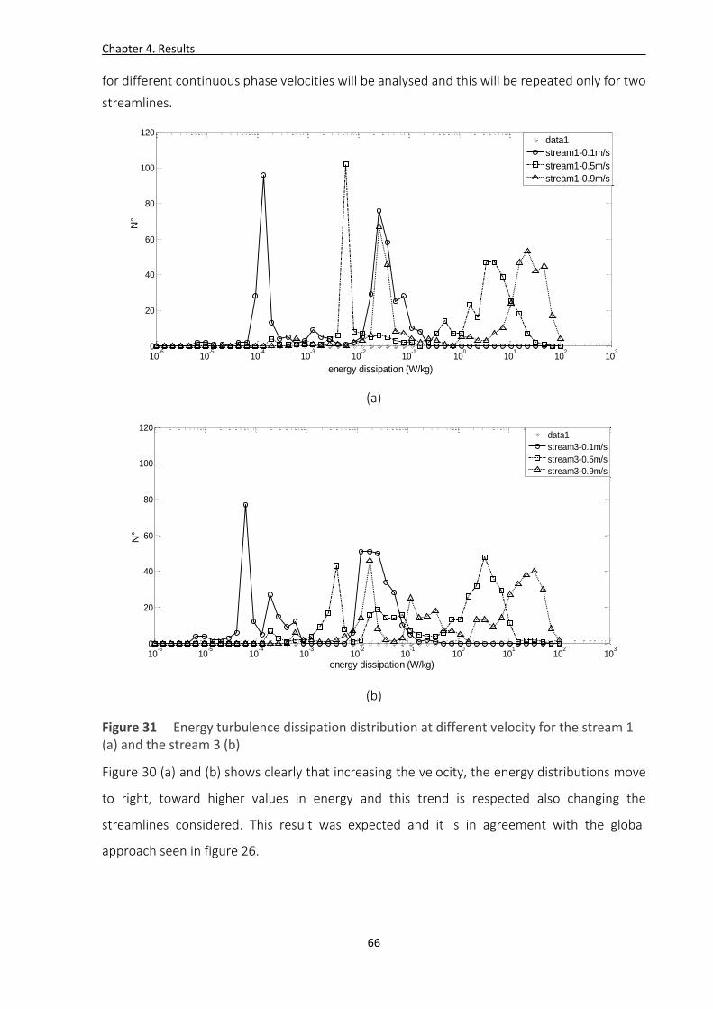
Chapter 4. Results
66
for different continuous phase velocities will be analysed and this will be repeated only for two
streamlines.
(a)
(b)
Figure 31 Energy turbulence dissipation distribution at different velocity for the stream 1 (a) and the stream 3 (b)
Figure 30 (a) and (b) shows clearly that increasing the velocity, the energy distributions move
to right, toward higher values in energy and this trend is respected also changing the
streamlines considered. This result was expected and it is in agreement with the global
approach seen in figure 26.
10-6
10-5
10-4
10-3
10-2
10-1
100
101
102
103
0
20
40
60
80
100
120
energy dissipation (W/kg)
N°
data1
stream1-0.1m/s
stream1-0.5m/s
stream1-0.9m/s
10-6
10-5
10-4
10-3
10-2
10-1
100
101
102
103
0
20
40
60
80
100
120
energy dissipation (W/kg)
N°
data1
stream3-0.1m/s
stream3-0.5m/s
stream3-0.9m/s

Chapter 4. Results
67
The same charts have been realized for the shear stress, in the figure below:
(a)
(b)
Figure 32 Shear stress distribution at different velocity for the stream 1 (a) and the stream 3 (b)
The shear stress distributions in figure 31 are referred on a specific streamline for different
continuous phase velocity. The charts show how increasing the velocity the shear stress
distributions are moving to right, toward higher values of the shear. This result was expected
and in agreement with the global approach which has shown that a linear relationship occurs
between shear stress and velocity.
All the data, which came from the streamline analysis presented until now, have shown that
both the shear stress and the energy turbulence dissipation enhance increasing the velocity,
according to the global approach (figure 26). Hence, in order to explain the weird values of the
shear stress measured on the drops surface (figure 26) another aspect should be investigated.
Indeed by using images came from the post-processing of the numerical simulations and
10-4
10-3
10-2
10-1
100
101
102
0
10
20
30
40
50
60
70
80
shear stress (Pa)
N°
data1
stream1-0.1m/s
stream1-0.5m/s
stream1-0.9m/s
10-4
10-3
10-2
10-1
100
101
102
0
10
20
30
40
50
60
70
80
shear stress(Pa)
N°
data1
stream3-0.1m/s
stream3-0.5m/s
stream3-0.9m/s
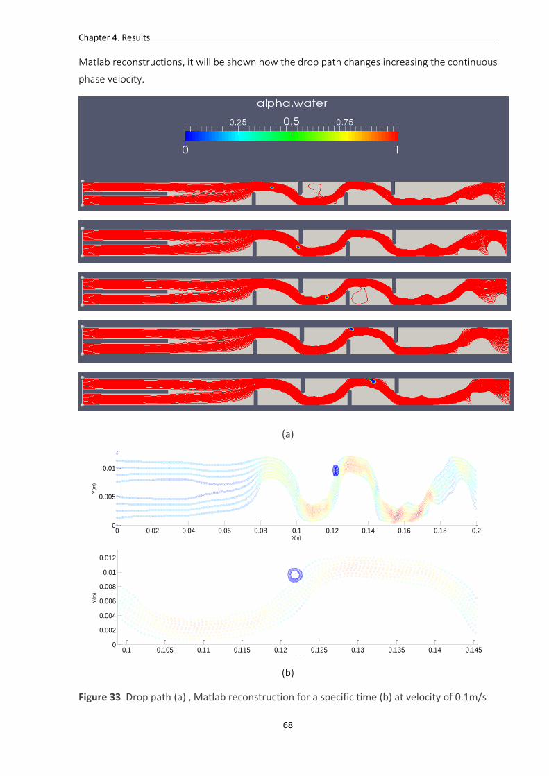
Chapter 4. Results
68
Matlab reconstructions, it will be shown how the drop path changes increasing the continuous
phase velocity.
(a)
(b)
Figure 33 Drop path (a) , Matlab reconstruction for a specific time (b) at velocity of 0.1m/s
0 0.02 0.04 0.06 0.08 0.1 0.12 0.14 0.16 0.18 0.20
0.005
0.01
X(m)
Y(m
)
0.1 0.105 0.11 0.115 0.12 0.125 0.13 0.135 0.14 0.1450
0.002
0.004
0.006
0.008
0.01
0.012
X(m)
Y(m
)
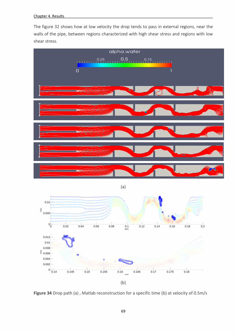
Chapter 4. Results
69
The figure 32 shows how at low velocity the drop tends to pass in external regions, near the
walls of the pipe, between regions characterized with high shear stress and regions with low
shear stress.
(a)
(b)
Figure 34 Drop path (a) , Matlab reconstruction for a specific time (b) at velocity of 0.5m/s
0 0.02 0.04 0.06 0.08 0.1 0.12 0.14 0.16 0.18 0.20
0.005
0.01
X(m)
Y(m
)
0.14 0.145 0.15 0.155 0.16 0.165 0.17 0.175 0.180
0.002
0.004
0.006
0.008
0.01
0.012
x(m)
Y(m
)
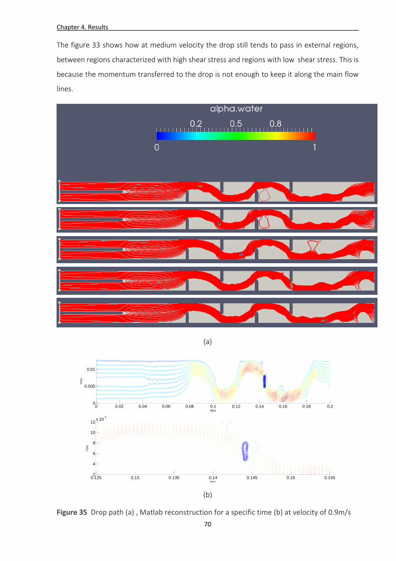
Chapter 4. Results
70
The figure 33 shows how at medium velocity the drop still tends to pass in external regions,
between regions characterized with high shear stress and regions with low shear stress. This is
because the momentum transferred to the drop is not enough to keep it along the main flow
lines.
(a)
(b)
Figure 35 Drop path (a) , Matlab reconstruction for a specific time (b) at velocity of 0.9m/s
0 0.02 0.04 0.06 0.08 0.1 0.12 0.14 0.16 0.18 0.20
0.005
0.01
X(m)
Y(m
)
0.125 0.13 0.135 0.14 0.145 0.15 0.1552
4
6
8
10
12x 10
-3
X(m)
Y(m
)
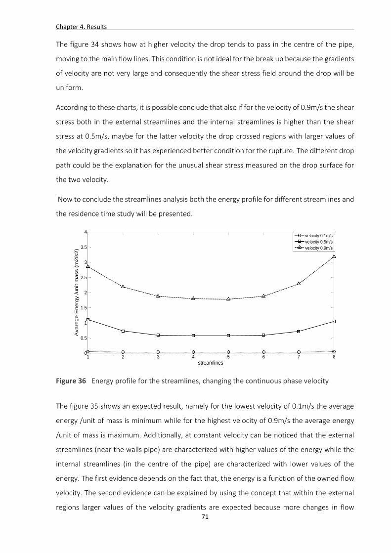
Chapter 4. Results
71
The figure 34 shows how at higher velocity the drop tends to pass in the centre of the pipe,
moving to the main flow lines. This condition is not ideal for the break up because the gradients
of velocity are not very large and consequently the shear stress field around the drop will be
uniform.
According to these charts, it is possible conclude that also if for the velocity of 0.9m/s the shear
stress both in the external streamlines and the internal streamlines is higher than the shear
stress at 0.5m/s, maybe for the latter velocity the drop crossed regions with larger values of
the velocity gradients so it has experienced better condition for the rupture. The different drop
path could be the explanation for the unusual shear stress measured on the drop surface for
the two velocity.
Now to conclude the streamlines analysis both the energy profile for different streamlines and
the residence time study will be presented.
Figure 36 Energy profile for the streamlines, changing the continuous phase velocity
The figure 35 shows an expected result, namely for the lowest velocity of 0.1m/s the average
energy /unit of mass is minimum while for the highest velocity of 0.9m/s the average energy
/unit of mass is maximum. Additionally, at constant velocity can be noticed that the external
streamlines (near the walls pipe) are characterized with higher values of the energy while the
internal streamlines (in the centre of the pipe) are characterized with lower values of the
energy. The first evidence depends on the fact that, the energy is a function of the owned flow
velocity. The second evidence can be explained by using the concept that within the external
regions larger values of the velocity gradients are expected because more changes in flow
1 2 3 4 5 6 7 80
0.5
1
1.5
2
2.5
3
3.5
4
streamlines
Avare
ge E
nerg
y /unit m
ass (
m2/s
2)
velocity 0.1m/s
velocity 0.5m/s
velocity 0.9m/s
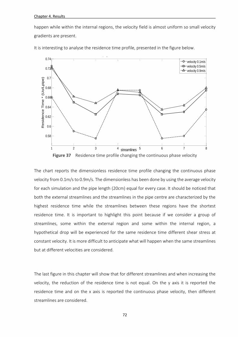
Chapter 4. Results
72
happen while within the internal regions, the velocity field is almost uniform so small velocity
gradients are present.
It is interesting to analyse the residence time profile, presented in the figure below.
Figure 37 Residence time profile changing the continuous phase velocity
The chart reports the dimensionless residence time profile changing the continuous phase
velocity from 0.1m/s to 0.9m/s. The dimensionless has been done by using the average velocity
for each simulation and the pipe length (20cm) equal for every case. It should be noticed that
both the external streamlines and the streamlines in the pipe centre are characterized by the
highest residence time while the streamlines between these regions have the shortest
residence time. It is important to highlight this point because if we consider a group of
streamlines, some within the external region and some within the internal region, a
hypothetical drop will be experienced for the same residence time different shear stress at
constant velocity. It is more difficult to anticipate what will happen when the same streamlines
but at different velocities are considered.
The last figure in this chapter will show that for different streamlines and when increasing the
velocity, the reduction of the residence time is not equal. On the y axis it is reported the
residence time and on the x axis is reported the continuous phase velocity, then different
streamlines are considered.
1 2 3 4 5 6 7 8
0.58
0.6
0.62
0.64
0.66
0.68
0.7
0.72
0.74
streamlines
Resid
ence T
ime *
(U
o/L
pip
e)
paragone dei residence Time adimensionale a diverse velocità
velocity 0.1m/s
velocity 0.5m/s
velocity 0.9m/s

Chapter 4. Results
73
Figure 38 Residence time profile for different velocity, changing the streamlines
It is possible to observe that at low velocity (0.1m/s) there is a larger difference in residence
time changing the streamline considered than the difference that exists for higher velocities
(0.5m/s and 0.9m/s).
0.1 0.2 0.3 0.4 0.5 0.6 0.7 0.8 0.90
0.2
0.4
0.6
0.8
1
1.2
1.4
velocity (m/s)
Resid
ence T
ime
stream1
stream2
stream3
stream4
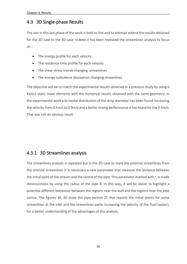
Chapter 4. Results
74
4.3 3D Single-phase Results
The aim in this last phase of the work is both to link and to attempt extend the results obtained
for the 2D case to the 3D case. Indeed it has been repeated the streamlines analysis to focus
on :
The energy profile for each velocity
The residence time profile for each velocity
The shear stress trends changing streamlines
The energy turbulence dissipation changing streamlines
The objective will be to match the experimental results obtained in a previous study by using 6
Kenics static mixer elements with the numerical results obtained with the same geometry. In
the experimental work a bi-modal distribution of the drop diameter has been found increasing
the velocity from 0.5m/s to 0.9m/s and a better mixing performance it has found for the 0.5m/s.
That was not an obvious result.
4.3.1 3D Streamlines analysis
The streamlines analysis is repeated but in the 3D case to mark the external streamlines from
the internal streamlines it is necessary a new parameter that measure the distance between
the initial point of the stream and the centre of the pipe. This parameter marked with r, is made
dimensionless by using the radius of the pipe R. In this way, it will be easier to highlight a
potential different behaviour between the regions near the wall and the regions near the pipe
centre. The figures 39, 40 show the pipe section ZY that reports the initial points for some
streamlines at the inlet and the streamlines paths increasing the velocity of the fluid (water),
for a better understanding of the advantages of this analysis.
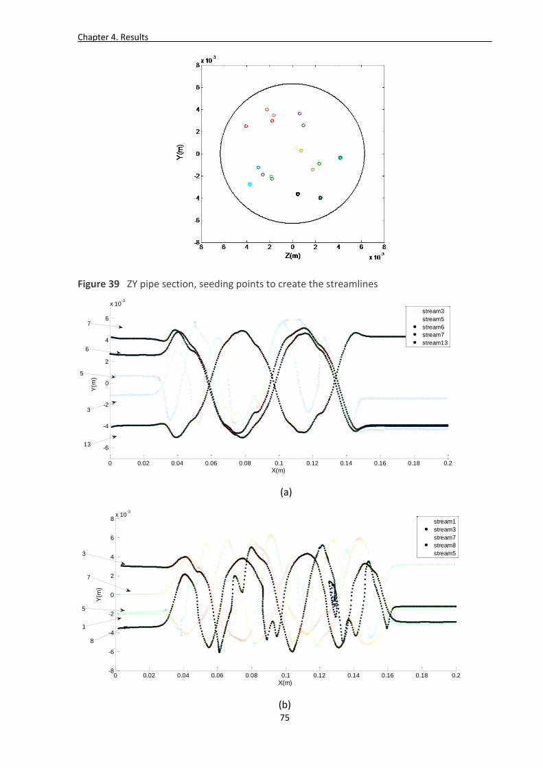
Chapter 4. Results
75
Figure 39 ZY pipe section, seeding points to create the streamlines
(a)
(b)
0 0.02 0.04 0.06 0.08 0.1 0.12 0.14 0.16 0.18 0.2
-6
-4
-2
0
2
4
6
x 10-3
X(m)
Y(m
)
stream3
stream5
stream6
stream7
stream13
13
3
5
6
7
0 0.02 0.04 0.06 0.08 0.1 0.12 0.14 0.16 0.18 0.2-8
-6
-4
-2
0
2
4
6
8x 10
-3
X(m)
Y(m
)
stream1
stream3
stream7
stream8
stream5
8
1
3
7
5
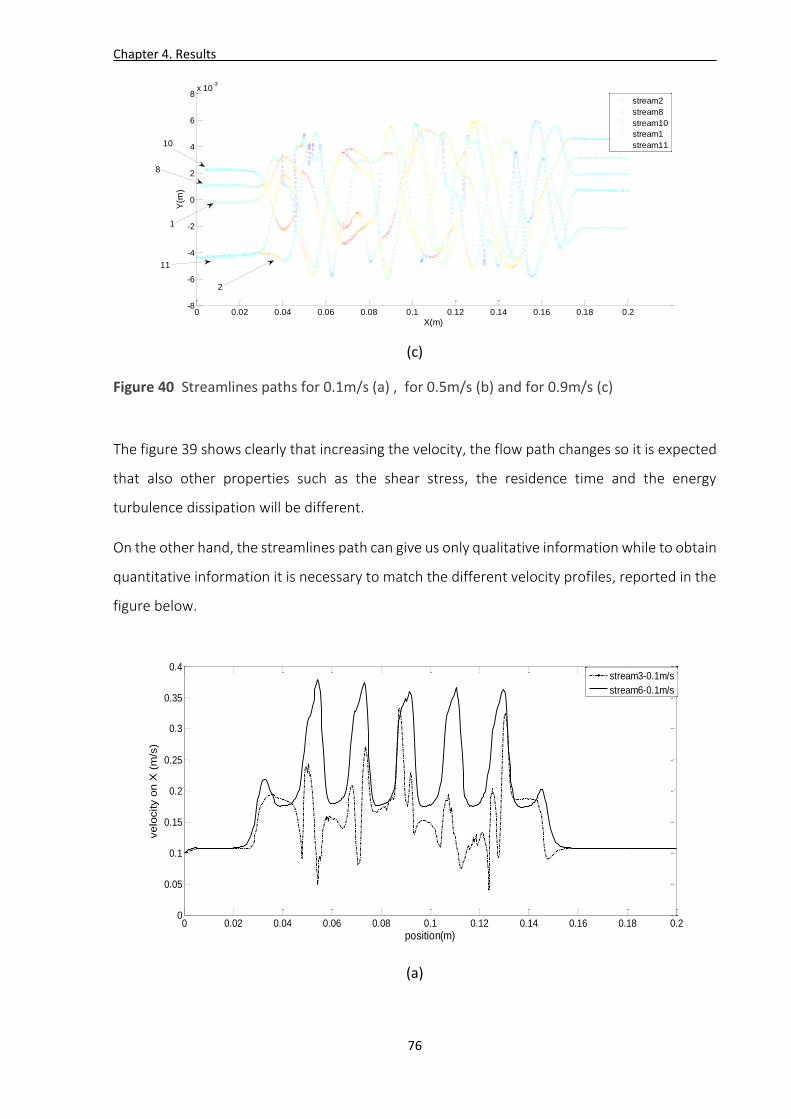
Chapter 4. Results
76
(c)
Figure 40 Streamlines paths for 0.1m/s (a) , for 0.5m/s (b) and for 0.9m/s (c)
The figure 39 shows clearly that increasing the velocity, the flow path changes so it is expected
that also other properties such as the shear stress, the residence time and the energy
turbulence dissipation will be different.
On the other hand, the streamlines path can give us only qualitative information while to obtain
quantitative information it is necessary to match the different velocity profiles, reported in the
figure below.
(a)
0 0.02 0.04 0.06 0.08 0.1 0.12 0.14 0.16 0.18 0.2-8
-6
-4
-2
0
2
4
6
8x 10
-3
X(m)
Y(m
)
stream2
stream8
stream10
stream1
stream11
1
11
2
8
10
0 0.02 0.04 0.06 0.08 0.1 0.12 0.14 0.16 0.18 0.20
0.05
0.1
0.15
0.2
0.25
0.3
0.35
0.4
position(m)
velo
city o
n X
(m
/s)
stream3-0.1m/s
stream6-0.1m/s
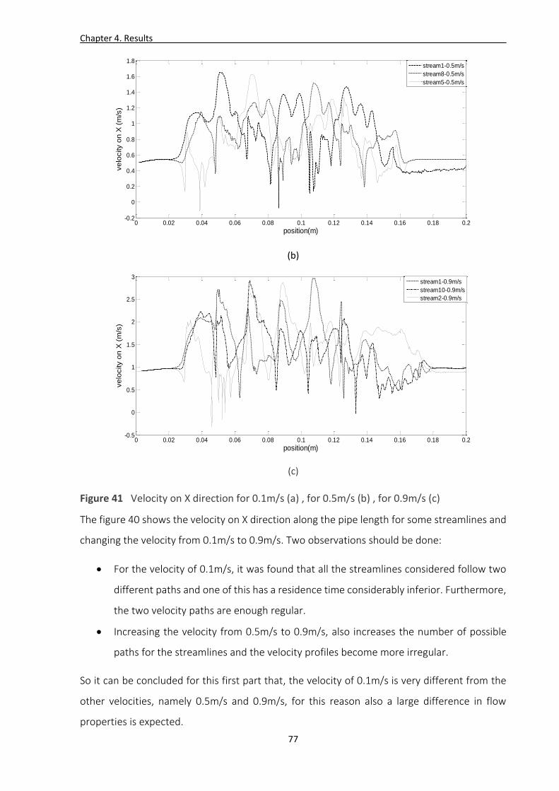
Chapter 4. Results
77
(b)
(c)
Figure 41 Velocity on X direction for 0.1m/s (a) , for 0.5m/s (b) , for 0.9m/s (c)
The figure 40 shows the velocity on X direction along the pipe length for some streamlines and
changing the velocity from 0.1m/s to 0.9m/s. Two observations should be done:
For the velocity of 0.1m/s, it was found that all the streamlines considered follow two
different paths and one of this has a residence time considerably inferior. Furthermore,
the two velocity paths are enough regular.
Increasing the velocity from 0.5m/s to 0.9m/s, also increases the number of possible
paths for the streamlines and the velocity profiles become more irregular.
So it can be concluded for this first part that, the velocity of 0.1m/s is very different from the
other velocities, namely 0.5m/s and 0.9m/s, for this reason also a large difference in flow
properties is expected.
0 0.02 0.04 0.06 0.08 0.1 0.12 0.14 0.16 0.18 0.2-0.2
0
0.2
0.4
0.6
0.8
1
1.2
1.4
1.6
1.8
position(m)
ve
locity o
n X
(m
/s)
stream1-0.5m/s
stream8-0.5m/s
stream5-0.5m/s
0 0.02 0.04 0.06 0.08 0.1 0.12 0.14 0.16 0.18 0.2-0.5
0
0.5
1
1.5
2
2.5
3
position(m)
ve
locity o
n X
(m
/s)
stream1-0.9m/s
stream10-0.9m/s
stream2-0.9m/s
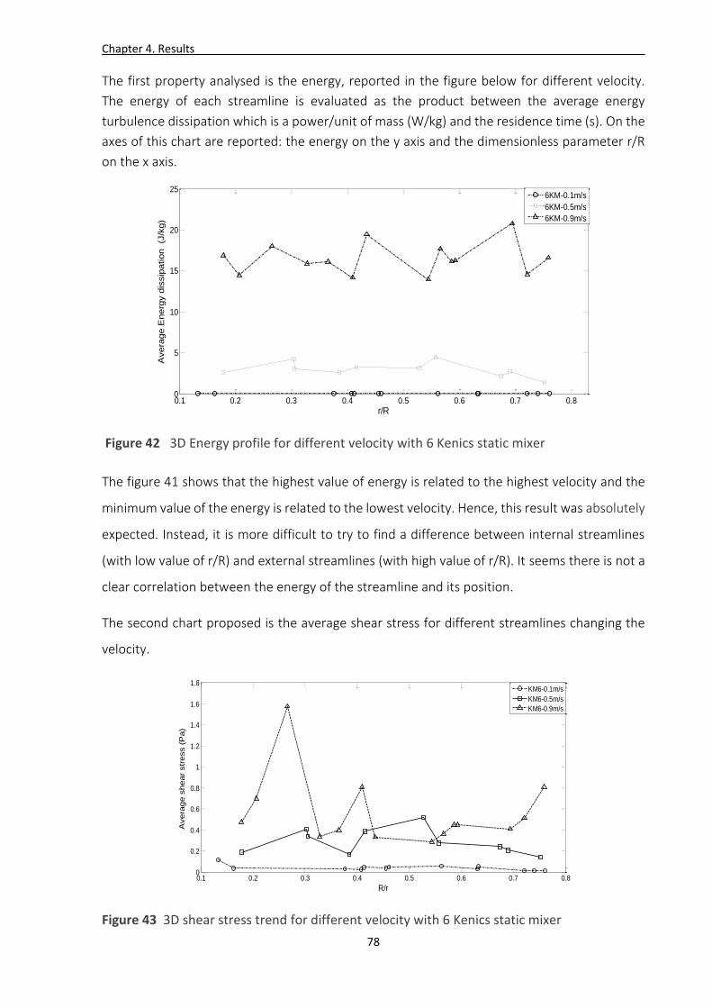
Chapter 4. Results
78
The first property analysed is the energy, reported in the figure below for different velocity.
The energy of each streamline is evaluated as the product between the average energy
turbulence dissipation which is a power/unit of mass (W/kg) and the residence time (s). On the
axes of this chart are reported: the energy on the y axis and the dimensionless parameter r/R
on the x axis.
Figure 42 3D Energy profile for different velocity with 6 Kenics static mixer
The figure 41 shows that the highest value of energy is related to the highest velocity and the
minimum value of the energy is related to the lowest velocity. Hence, this result was absolutely
expected. Instead, it is more difficult to try to find a difference between internal streamlines
(with low value of r/R) and external streamlines (with high value of r/R). It seems there is not a
clear correlation between the energy of the streamline and its position.
The second chart proposed is the average shear stress for different streamlines changing the
velocity.
Figure 43 3D shear stress trend for different velocity with 6 Kenics static mixer
0.1 0.2 0.3 0.4 0.5 0.6 0.7 0.80
5
10
15
20
25
r/R
Avera
ge E
nerg
y d
issip
ation (J
/kg)
6KM-0.1m/s
6KM-0.5m/s
6KM-0.9m/s
0.1 0.2 0.3 0.4 0.5 0.6 0.7 0.80
0.2
0.4
0.6
0.8
1
1.2
1.4
1.6
1.8
R/r
Avera
ge s
hear
str
ess (
Pa)
KM6-0.1m/s
KM6-0.5m/s
KM6-0.9m/s
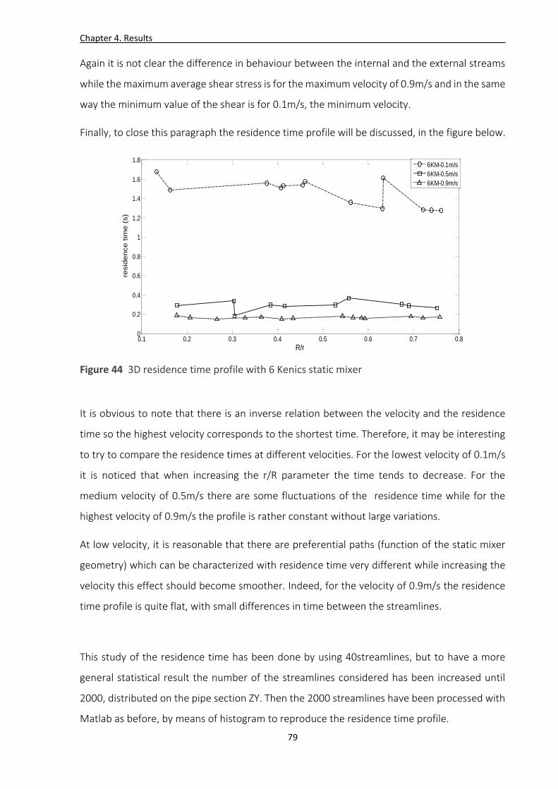
Chapter 4. Results
79
Again it is not clear the difference in behaviour between the internal and the external streams
while the maximum average shear stress is for the maximum velocity of 0.9m/s and in the same
way the minimum value of the shear is for 0.1m/s, the minimum velocity.
Finally, to close this paragraph the residence time profile will be discussed, in the figure below.
Figure 44 3D residence time profile with 6 Kenics static mixer
It is obvious to note that there is an inverse relation between the velocity and the residence
time so the highest velocity corresponds to the shortest time. Therefore, it may be interesting
to try to compare the residence times at different velocities. For the lowest velocity of 0.1m/s
it is noticed that when increasing the r/R parameter the time tends to decrease. For the
medium velocity of 0.5m/s there are some fluctuations of the residence time while for the
highest velocity of 0.9m/s the profile is rather constant without large variations.
At low velocity, it is reasonable that there are preferential paths (function of the static mixer
geometry) which can be characterized with residence time very different while increasing the
velocity this effect should become smoother. Indeed, for the velocity of 0.9m/s the residence
time profile is quite flat, with small differences in time between the streamlines.
This study of the residence time has been done by using 40streamlines, but to have a more
general statistical result the number of the streamlines considered has been increased until
2000, distributed on the pipe section ZY. Then the 2000 streamlines have been processed with
Matlab as before, by means of histogram to reproduce the residence time profile.
0.1 0.2 0.3 0.4 0.5 0.6 0.7 0.80
0.2
0.4
0.6
0.8
1
1.2
1.4
1.6
1.8
R/r
resid
ence tim
e (
s)
6KM-0.1m/s
6KM-0.5m/s
6KM-0.9m/s
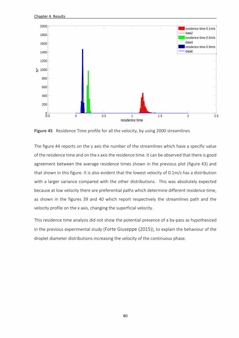
Chapter 4. Results
80
Figure 45 Residence Time profile for all the velocity, by using 2000 streamlines
The figure 44 reports on the y axis the number of the streamlines which have a specific value
of the residence time and on the x axis the residence time. It can be observed that there is good
agreement between the average residence times shown in the previous plot (figure 43) and
that shown in this figure. It is also evident that the lowest velocity of 0.1m/s has a distribution
with a larger variance compared with the other distributions. This was absolutely expected
because at low velocity there are preferential paths which determine different residence time,
as shown in the figures 39 and 40 which report respectively the streamlines path and the
velocity profile on the x axis, changing the superficial velocity.
This residence time analysis did not show the potential presence of a by-pass as hypothesized
in the previous experimental study (Forte Giuseppe (2015)), to explain the behaviour of the
droplet diameter distributions increasing the velocity of the continuous phase.
-0.5 0 0.5 1 1.5 2 2.50
200
400
600
800
1000
1200
1400
1600
1800
2000
residence time
N°
residence time-0.1m/s
data2
residence time-0.5m/s
data4
residence time-0.9m/s
data6
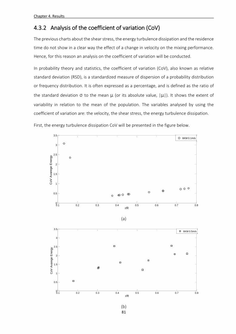
Chapter 4. Results
81
4.3.2 Analysis of the coefficient of variation (CoV)
The previous charts about the shear stress, the energy turbulence dissipation and the residence
time do not show in a clear way the effect of a change in velocity on the mixing performance.
Hence, for this reason an analysis on the coefficient of variation will be conducted.
In probability theory and statistics, the coefficient of variation (CoV), also known as relative
standard deviation (RSD), is a standardized measure of dispersion of a probability distribution
or frequency distribution. It is often expressed as a percentage, and is defined as the ratio of
the standard deviation σ to the mean µ (or its absolute value, |µ|). It shows the extent of
variability in relation to the mean of the population. The variables analysed by using the
coefficient of variation are: the velocity, the shear stress, the energy turbulence dissipation.
First, the energy turbulence dissipation CoV will be presented in the figure below.
(a)
(b)
0.1 0.2 0.3 0.4 0.5 0.6 0.7 0.80
0.5
1
1.5
2
2.5
3
3.5
r/R
CoV
Avare
ge E
nerg
y
6KM 0.1m/s
0.1 0.2 0.3 0.4 0.5 0.6 0.7 0.80
0.5
1
1.5
2
2.5
3
3.5
r/R
CoV
Avare
ge E
nerg
y
6KM 0.5m/s
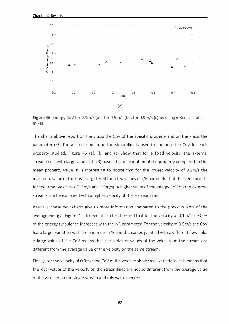
Chapter 4. Results
82
(c)
Figure 46 Energy CoV for 0.1m/s (a) , for 0.5m/s (b) , for 0.9m/s (c) by using 6 Kenics static mixer
The charts above report on the y axis the CoV of the specific property and on the x axis the
parameter r/R. The absolute mean on the streamline is used to compute the CoV for each
property studied. Figure 45 (a), (b) and (c) show that for a fixed velocity, the external
streamlines (with large values of r/R) have a higher variation of the property compared to the
mean property value. It is interesting to notice that for the lowest velocity of 0.1m/s the
maximum value of the CoV is registered for a low values of r/R parameter but the trend inverts
for the other velocities (0.5m/s and 0.9m/s). A higher value of the energy CoV on the external
streams can be explained with a higher velocity of these streamlines.
Basically, these new charts give us more information compared to the previous plots of the
average energy ( Figure41 ). Indeed, it can be observed that for the velocity of 0.1m/s the CoV
of the energy turbulence increases with the r/R parameter. For the velocity of 0.5m/s the CoV
has a larger variation with the parameter r/R and this can be justified with a different flow field.
A large value of the CoV means that the series of values of the velocity on the stream are
different from the average value of the velocity on the same stream.
Finally, for the velocity of 0.9m/s the CoV of the velocity show small variations, this means that
the local values of the velocity on the streamlines are not so different from the average value
of the velocity on the single stream and this was expected.
0.1 0.2 0.3 0.4 0.5 0.6 0.7 0.80
0.5
1
1.5
2
2.5
3
3.5
r/R
CoV
Avare
ge E
nerg
y
6KM-0.9m/s
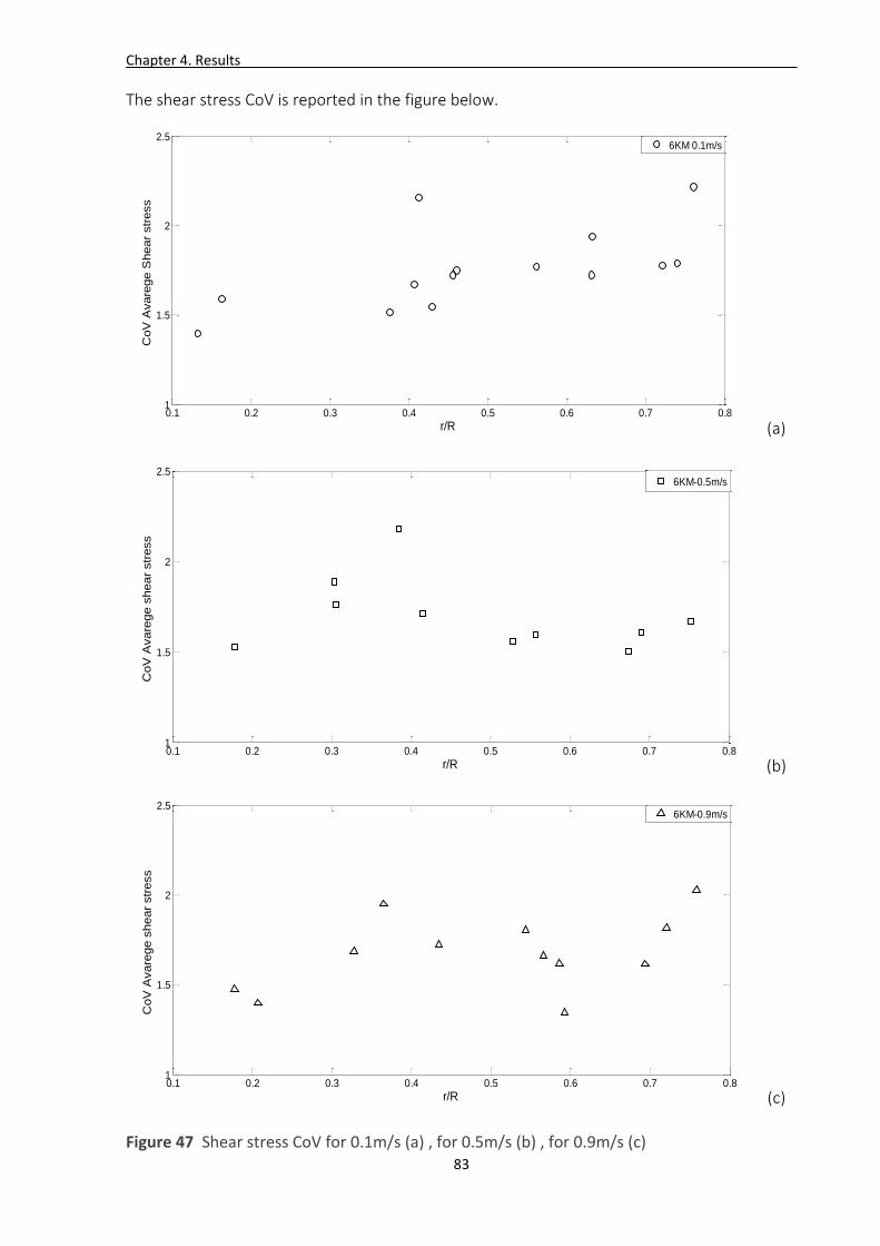
Chapter 4. Results
83
The shear stress CoV is reported in the figure below.
(a)
(b)
(c)
Figure 47 Shear stress CoV for 0.1m/s (a) , for 0.5m/s (b) , for 0.9m/s (c)
0.1 0.2 0.3 0.4 0.5 0.6 0.7 0.81
1.5
2
2.5
r/R
CoV
Avare
ge S
hear
str
ess
6KM 0.1m/s
0.1 0.2 0.3 0.4 0.5 0.6 0.7 0.81
1.5
2
2.5
r/R
CoV
Avare
ge s
hear
str
ess
6KM-0.5m/s
0.1 0.2 0.3 0.4 0.5 0.6 0.7 0.81
1.5
2
2.5
r/R
CoV
Avare
ge s
hear
str
ess
6KM-0.9m/s

Chapter 4. Results
84
Figure 46 shows that for 0.1m/s and 0.9m/s the CoV of the shear stress increases with the r/R
parameter while a different behaviour is shown for the 0.5m/s where there is not a clear trend.
Comparing all the velocities together it can be seen that the higher values of the CoV belong to
the lowest velocity, namely 0.1m/s. This can be explained with a lower uniformity of the velocity
field compare with the other velocities where the velocity field tends to be more uniform, with
a central region at high velocity and an external region at low velocity.
Finally, the velocity CoV is reported in the figure below.
(a)
(b)
0.1 0.2 0.3 0.4 0.5 0.6 0.7 0.80.25
0.3
0.35
0.4
0.45
0.5
0.55
0.6
0.65
0.7
r/R
CoV
Avare
ge U
x
6KM-0.1m/s
0.1 0.2 0.3 0.4 0.5 0.6 0.7 0.80.25
0.3
0.35
0.4
0.45
0.5
0.55
0.6
0.65
0.7
r/R
CoV
Avare
ge U
x
6KM-0.5m/s

Chapter 4. Results
85
(c)
Figure 48 The velocity CoV for 0.1m/s (a), for the 0.5m/s (b) , for the 0.9m/s (c) , by using 6 Kenics static mixer
Figure 47 shows for the velocities of 0.1m/s and 0.5m/s that, the CoV is higher for the external
streamlines than the internal streams while this trend is not evident for the velocity of 0.9m/s.
This can be explained thinking that the velocity gradients are not too large at 0.9m/s because
the flow field is relatively uniform.
The analysis of the coefficient of variation can be concluded observing that there were higher
values of the CoV of the properties for the external streamlines compared to the internal
streams. This is not surprising because the external regions take account of the wall effects.
4.3.3 3D flow field
To conclude the chapter of the results, images of the 3D flow field will be show to highlight the
difference existing increasing the velocity, then finally, the stream path will be observed by
using the section pipe ZY to attempt to understand the effect of the velocity on a hypothetical
mixing.
0.1 0.2 0.3 0.4 0.5 0.6 0.7 0.80.25
0.3
0.35
0.4
0.45
0.5
0.55
0.6
0.65
0.7
r/R
CoV
Avare
ge U
x
6KM-0.9m/s
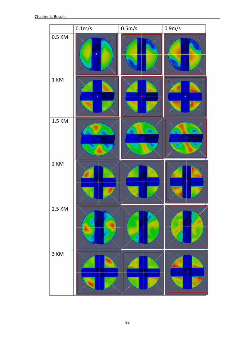
Chapter 4. Results
86
0.1m/s 0.5m/s 0.9m/s
0.5 KM
1 KM
1.5 KM
2 KM
2.5 KM
3 KM

Chapter 4. Results
87
3.5 KM
4 KM
4.5 KM
5 KM
5.5 KM
6 KM
Figure 49 3D velocity field with 6 Kenics static mixer (Magnitude of the velocity)
Chapter 4. Results
88
In the images reported above, for each half of the static mixer a section pipe is reported to
analyse the flow field and its development. The figure 48 shows that there is an evident
difference between the structure of the velocity field at 0.1m/s and those at 0.5m/s and 0.9m/s.
Indeed, a flow transition can be observed between these range of velocity. It should be noticed
that:
The static mixer configuration makes the structure of the flow repeatable, indeed for
the section of the element 1,3,5 or 2,4 or 0.5, 2.5, 4.5 the flow is exactly the same.
Increasing the velocity from 0.5m/s to 0.9m/s the flow quality is the same. The flow
structure does not change but what changes is the magnitude of the velocity.
The last data collection will show the streamline path across the pipe section ZY, for a better
understanding of how the mixing can develop from the pipe centre to the pipe walls. Indeed,
in the following images streamlines with similar values of the parameter r/R will be compared,
for different velocities.
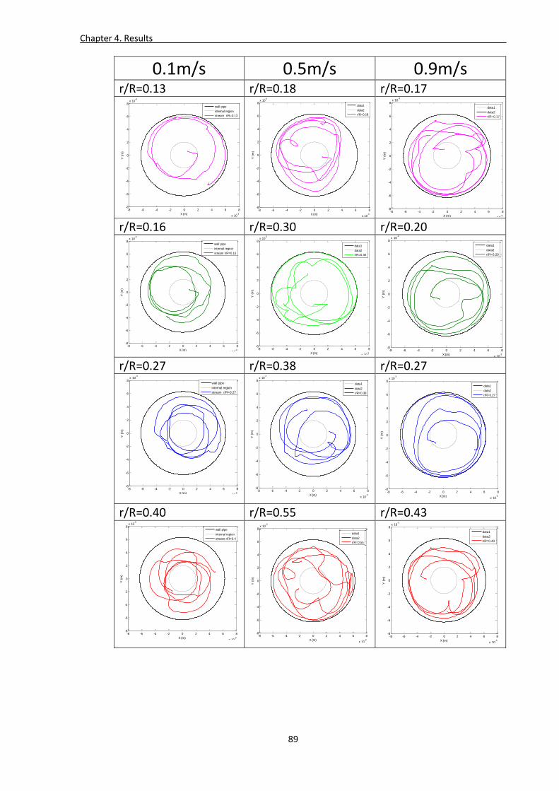
Chapter 4. Results
89
0.1m/s 0.5m/s 0.9m/s r/R=0.13 r/R=0.18 r/R=0.17
r/R=0.16 r/R=0.30 r/R=0.20
r/R=0.27 r/R=0.38 r/R=0.27
r/R=0.40 r/R=0.55 r/R=0.43
-8 -6 -4 -2 0 2 4 6 8
x 10-3
-8
-6
-4
-2
0
2
4
6
8x 10
-3
X (m)
Y (
m)
wall pipe
internal region
stream r/R=0.13
-8 -6 -4 -2 0 2 4 6 8
x 10-3
-8
-6
-4
-2
0
2
4
6
8x 10
-3
X (m)
Y (
m)
data1
data2
r/R=0.18
-8 -6 -4 -2 0 2 4 6 8
x 10-3
-8
-6
-4
-2
0
2
4
6
8x 10
-3
X (m)
Y (
m)
data1
data2
r/R=0.17
-8 -6 -4 -2 0 2 4 6 8
x 10-3
-8
-6
-4
-2
0
2
4
6
8x 10
-3
X (m)
Y (
m)
wall pipe
internal region
stream r/R=0.16
-8 -6 -4 -2 0 2 4 6 8
x 10-3
-8
-6
-4
-2
0
2
4
6
8x 10
-3
X (m)
Y (
m)
data1
data2
r/R=0.30
-8 -6 -4 -2 0 2 4 6 8
x 10-3
-8
-6
-4
-2
0
2
4
6
8x 10
-3
X (m)
Y (
m)
data1
data2
r/R=0.20
-8 -6 -4 -2 0 2 4 6 8
x 10-3
-8
-6
-4
-2
0
2
4
6
8x 10
-3
X (m)
Y (
m)
wall pipe
internal region
stream r/R=0.27
-8 -6 -4 -2 0 2 4 6 8
x 10-3
-8
-6
-4
-2
0
2
4
6
8x 10
-3
X (m)
Y (
m)
data1
data2
r/R=0.38
-8 -6 -4 -2 0 2 4 6 8
x 10-3
-8
-6
-4
-2
0
2
4
6
8x 10
-3
X (m)
Y (
m)
data1
data2
r/R=0.27
-8 -6 -4 -2 0 2 4 6 8
x 10-3
-8
-6
-4
-2
0
2
4
6
8x 10
-3
X (m)
Y (
m)
wall pipe
internal region
stream r/R=0.4
-8 -6 -4 -2 0 2 4 6 8
x 10-3
-8
-6
-4
-2
0
2
4
6
8x 10
-3
X (m)
Y (
m)
data1
data2
r/R=0.55
-8 -6 -4 -2 0 2 4 6 8
x 10-3
-8
-6
-4
-2
0
2
4
6
8x 10
-3
X (m)
Y (
m)
data1
data2
r/R=0.43
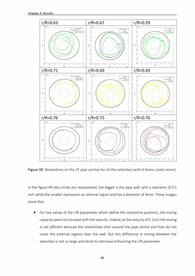
Chapter 4. Results
90
r/R=0.63 r/R=0.67 r/R=0.59
r/R=0.71 r/R=0.69 r/R=0.69
r/R=0.76 r/R=0.75 r/R=0.76
Figure 50 Streamlines on the ZY pipe section for all the velocities (with 6 Kenics static mixer)
In the figure 49 two circles are represented, the bigger is the pipe wall, with a diameter of 0.5
inch while the smaller represents an internal region and has a diameter of 4mm. These images
show that:
For low values of the r/R (parameter which define the streamline position), the mixing
capacity seems to increase with the velocity. Indeed, at the velocity of 0.1m/s the mixing
is not efficient because the streamlines start around the pipe centre and then do not
cover the external regions near the wall. But this difference in mixing between the
velocities is not so large and tends to decrease enhancing the r/R parameter.
-8 -6 -4 -2 0 2 4 6 8
x 10-3
-8
-6
-4
-2
0
2
4
6
8x 10
-3
X (m)
Y (
m)
internal region
wal pipe
stream r/R=0.63
-8 -6 -4 -2 0 2 4 6 8
x 10-3
-8
-6
-4
-2
0
2
4
6
8x 10
-3
X (m)
Y (
m)
data1
data2
r/R=0.67
-8 -6 -4 -2 0 2 4 6 8
x 10-3
-8
-6
-4
-2
0
2
4
6
8x 10
-3
X (m)
Y (
m)
data1
data2
r/R=0.59
-8 -6 -4 -2 0 2 4 6 8
x 10-3
-8
-6
-4
-2
0
2
4
6
8x 10
-3
X (m)
Y (
m)
wall pipe
internal region
stream r/R=0.71
-8 -6 -4 -2 0 2 4 6 8
x 10-3
-8
-6
-4
-2
0
2
4
6
8x 10
-3
X (m)
Y (
m)
data1
data2
r/R=0.69
-8 -6 -4 -2 0 2 4 6 8
x 10-3
-8
-6
-4
-2
0
2
4
6
8x 10
-3
X (m)
Y (
m)
data1
data2
r/R=0.69
-8 -6 -4 -2 0 2 4 6 8
x 10-3
-8
-6
-4
-2
0
2
4
6
8x 10
-3
X (m)
Y (
m)
wall pipe
internal region
stream r/R=0.76
-8 -6 -4 -2 0 2 4 6 8
x 10-3
-8
-6
-4
-2
0
2
4
6
8x 10
-3
X (m)
Y (
m)
data1
data2
r/R=0.75
-8 -6 -4 -2 0 2 4 6 8
x 10-3
-8
-6
-4
-2
0
2
4
6
8x 10
-3
data1
data2
r/R=0.76
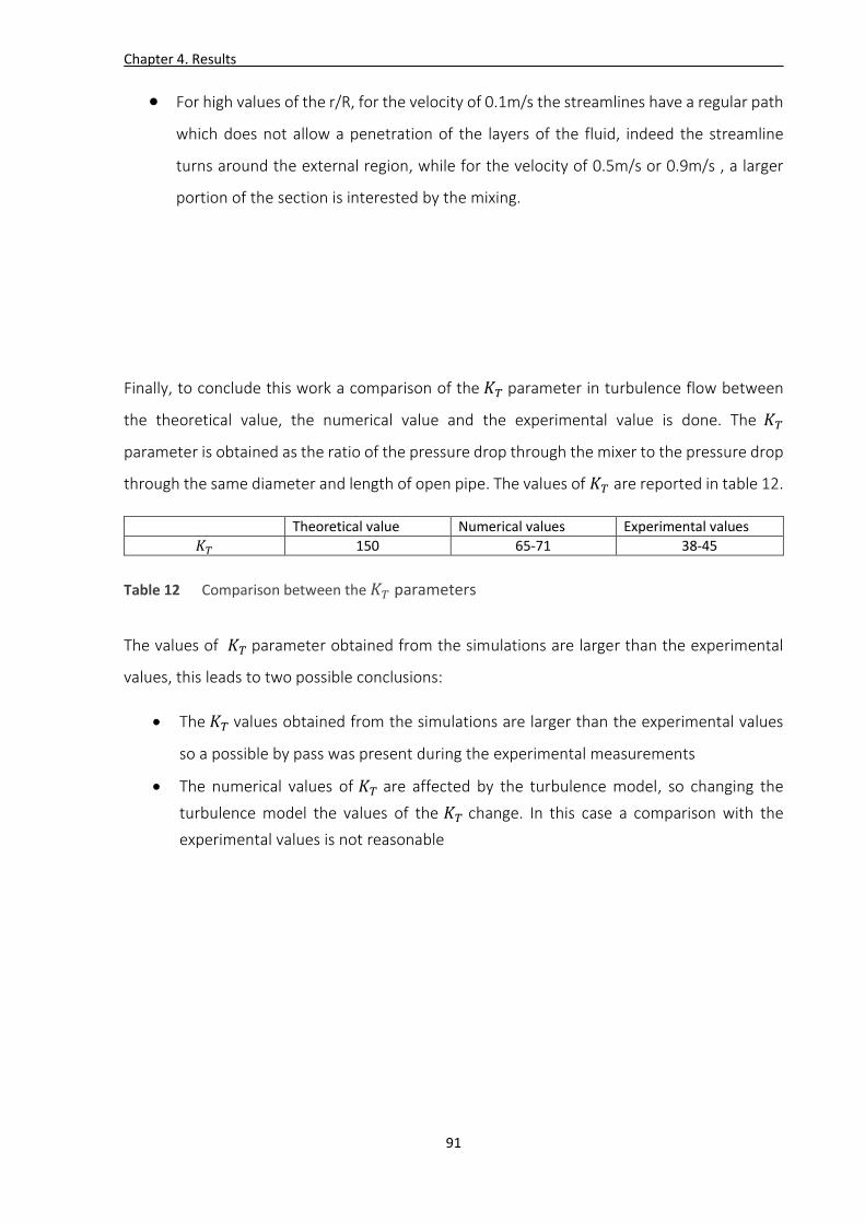
Chapter 4. Results
91
For high values of the r/R, for the velocity of 0.1m/s the streamlines have a regular path
which does not allow a penetration of the layers of the fluid, indeed the streamline
turns around the external region, while for the velocity of 0.5m/s or 0.9m/s , a larger
portion of the section is interested by the mixing.
Finally, to conclude this work a comparison of the 𝐾𝑇 parameter in turbulence flow between
the theoretical value, the numerical value and the experimental value is done. The 𝐾𝑇
parameter is obtained as the ratio of the pressure drop through the mixer to the pressure drop
through the same diameter and length of open pipe. The values of 𝐾𝑇 are reported in table 12.
Theoretical value Numerical values Experimental values
𝐾𝑇 150 65-71 38-45
Table 12 Comparison between the 𝐾𝑇 parameters
The values of 𝐾𝑇 parameter obtained from the simulations are larger than the experimental
values, this leads to two possible conclusions:
The 𝐾𝑇 values obtained from the simulations are larger than the experimental values
so a possible by pass was present during the experimental measurements
The numerical values of 𝐾𝑇 are affected by the turbulence model, so changing the
turbulence model the values of the 𝐾𝑇 change. In this case a comparison with the
experimental values is not reasonable

92
Chapter 5
Conclusions
In this work, static mixer performance in mixing of immiscible fluids has been investigated by
using a numerical approach. Several simulations have been performed during this research
work, by means of the open source platform OpenFoam. Simulations have investigated the
mixing performance, exploring the effect of the continuous phase velocity on the disperse
phase. Indeed, the velocity was ranging from 0.1m/s to 0.9m/s. The static mixer geometry
tested has been the Kenics (KM) 6 elements, realized with the open source software Salome
7.5.1 . Basically, for a better understand of the mixing of immiscible fluids two properties have
been studied: the energy turbulence dissipation and the shear stress, because both the
properties can be linked with the break up mechanisms.
In the paragraph 4.2.1 the 2D results are presented, starting with the study of the drop surface,
in order to observe the shear stress and the energy turbulence dissipation, by using a Matlab
reconstruction of the drop. Basically, this local approach has found that the shear stress as the
energy turbulence dissipation increases with the drop deformation and with the velocity of the
continuous phase in a different way. Indeed for the shear stress, it was found that it increases
with the drop deformation and it is not linear with the velocity, because the better shear stress
conditions are at 0.5m/s and not 0.9m/s which is the highest velocity. This result can be linked
with the experimental results obtained in a previous study, but need further explanation. For
the energy turbulence dissipation, a linear relation with the velocity was found, while a linear
relation with the drop deformation does not exist. This result is not surprising because basically
the energy is a function of the turbulence intensity which increases with the velocity. To clarify
the result obtained for the shear stress valuated on the drop surfaces, a global approach is
used, by means of a histogram of the shear stress computed in all the points of the geometry.
This different approach leads to the conclusion that the shear stress should increase in a linear
way with the velocity, but this was expected because the break up of the drop is a local
phenomenon which can be lost with a global statistical approach.

Chapter 5. Conclusions
93
In the paragraph 4.2.2 a streamlines analysis is conducted with the aim to confirm the shear
stress trend found when analysing the drop surface and at the same time to attempt to link the
drop position in the velocity field with the break up conditions. The analysis of single
streamlines for different velocity has shown that:
Increasing the continuous phase velocity, properties such as the shear stress and the
energy turbulence dissipation increase, confirming the previous results obtained from
the global approach
By using enough streamlines along the pipe length, it was shown that the drop path
changes increasing the velocity. Indeed, at low velocity the drop crosses external
regions, with large velocity gradients and so a higher shear stress. While at the high
velocity, the drop tends to move to the centre pipe, where the gradients are smaller
because the velocity fields is quite uniform.
Furthermore, by means the residence time, it has found that the streamlines near the wall have
longer time compared to the streams near the centre pipe. This means that also if the shear
stress conditions could be permit the rupture of the drop, a mechanical equilibrium should be
taken into account.
In the paragraph 4.3 the 3D results are presented and the streamlines analysis is repeated, in
order to attempt to confirm or extend the 2D results. The streamlines results do not show for
the properties such as the shear stress and the energy turbulence dissipation a clear behaviour
increasing the r/R parameter (which define the stream position). Hence, a further analysis of
the coefficient of variation is done. This analysis leads to the conclusion that increasing the r/R
parameter the shear stress and the energy turbulence dissipation tend to increase. So as for
the 2D analysis, it was found that the external streams involve larger variation in the properties
compared to the internal streams. Finally, the 3D velocity field is shown and additionally, the
path of the streamlines across the ZY pipe section, give us a better idea of the mixing efficiency
increasing the velocity. Indeed, it noticed that above certain values of r/R parameter ( >0.65)
at low velocity the stream follows a regular path and does not cross from the external region
to the centre of pipe. Furthermore, by increasing the velocity, better mixing is obtained, with
streams which interest a large part of the pipe section. Instead, for low values of r/R parameter,
by increasing the velocity an improvement in the mixing can be observed, but it is not possible
to quantify how much the mixing at 0.9m/s is better than that at 0.5m/s or vice versa.
Chapter 5. Conclusions
94
5.1 Future work
Further simulations could enhance the consistency of the numerical model and integrate it. It
would be useful to repeat the simulations raising the number of elements or testing different
static mixer geometry, as the Sulzer SMX plus. It could be very interesting to perform the same
3D geometry but by using a multi-phase model to trace the oil drop along the pipe and to
attempt to extend the 2D multi-phase results obtained with this work. The principal obstacle is
the computational costs required, which limit the possible applications and the difficulties to
transfer large data for the post-processing of the numerical solution.

Appendix A . OpenFoam file
95
Appendix A
OpenFoam Turbulence Model ( 2D Multi-phase model)
/*--------------------------------*- C++ -*----------------------------------*\
| ========= | |
| \\ / F ield | OpenFOAM: The Open Source CFD Toolbox |
| \\ / O peration | Version: 2.3.1 |
| \\ / A nd | Web: www.OpenFOAM.org |
| \\/ M anipulation | |
\*---------------------------------------------------------------------------*/
FoamFile
{
version 2.0;
format ascii;
class dictionary;
location "constant";
object turbulenceProperties;
}
// * * * * * * * * * * * * * * * * * * * * * * * * * * * * * * * * * *
* * * //
simulationType RASModel;
//
***********************************************************************
** //
OpenFoam Turbulence Properties ( 2D Multi-phase model)
/*--------------------------------*- C++ -*----------------------------------*\
| ========= | |
| \\ / F ield | OpenFOAM: The Open Source CFD Toolbox |
| \\ / O peration | Version: 2.3.1 |
| \\ / A nd | Web: www.OpenFOAM.org |
| \\/ M anipulation | |
\*---------------------------------------------------------------------------*/
FoamFile
{
version 2.0;
format ascii;
class dictionary;
location "constant";
object transportProperties;
}
// * * * * * * * * * * * * * * * * * * * * * * * * * * * * * * * * * *
* * * //
phases (water oil);
water
{

Appendix A . OpenFoam file
96
transportModel Newtonian;
nu nu [ 0 2 -1 0 0 0 0 ] 1e-06;
rho rho [ 1 -3 0 0 0 0 0 ] 1000;
}
oil
{
transportModel Newtonian;
nu nu [ 0 2 -1 0 0 0 0 ] 4e-06;
rho rho [ 1 -3 0 0 0 0 0 ] 800;
}
sigma sigma [ 1 0 -2 0 0 0 0 ] 0.02267;
//
***********************************************************************
** //
OpenFoam RAS Properties ( 2D Multi-phase model)
/*--------------------------------*- C++ -*----------------------------------*\
| ========= | |
| \\ / F ield | OpenFOAM: The Open Source CFD Toolbox |
| \\ / O peration | Version: 2.3.1 |
| \\ / A nd | Web: www.OpenFOAM.org |
| \\/ M anipulation | |
\*---------------------------------------------------------------------------*/
FoamFile
{
version 2.0;
format ascii;
class dictionary;
location "constant";
object RASProperties;
}
// * * * * * * * * * * * * * * * * * * * * * * * * * * * * * * * * * *
* * * //
RASModel kOmegaSST;
turbulence on;
printCoeffs on;
//
***********************************************************************
** //

Appendix A . OpenFoam file
97
ControlDict file ( 2D Multi-phase model)
/*--------------------------------*- C++ -*----------------------------------*\
| ========= | |
| \\ / F ield | OpenFOAM: The Open Source CFD Toolbox |
| \\ / O peration | Version: 2.3.1 |
| \\ / A nd | Web: www.OpenFOAM.org |
| \\/ M anipulation | |
\*---------------------------------------------------------------------------*/
FoamFile
{
version 2.0;
format ascii;
class dictionary;
location "system";
object controlDict;
}
// * * * * * * * * * * * * * * * * * * * * * * * * * * * * * * * * * * * * * //
application LTSInterFoam;
startFrom startTime;
startTime 10;
stopAt endTime;
endTime 12; // il tempo di attraversamento è 0.4s con
Vw=0.5m/s
deltaT 1e-4;
writeControl adjustableRunTime;
writeInterval 0.05; //modificato
purgeWrite 0;
writeFormat ascii;
writePrecision 6;
writeCompression uncompressed;
timeFormat general;
timePrecision 6;
runTimeModifiable yes; //se modifico il file dict vedo le modifiche in
tempo reale
adjustTimeStep on;
maxCo 0.5; //cambiato manualmente prima era 1
maxAlphaCo 0.5; //cambiato manualmente prima era 1
maxDeltaT 1;
//
***********************************************************************
** //

Appendix A . OpenFoam file
98
FvSchemes file ( 2D Multi-phase model)
/*--------------------------------*- C++ -*----------------------------------*\
| ========= | |
| \\ / F ield | OpenFOAM: The Open Source CFD Toolbox |
| \\ / O peration | Version: 2.3.1 |
| \\ / A nd | Web: www.OpenFOAM.org |
| \\/ M anipulation | |
\*---------------------------------------------------------------------------*/
FoamFile
{
version 2.0;
format ascii;
class dictionary;
location "system";
object fvSchemes;
}
// * * * * * * * * * * * * * * * * * * * * * * * * * * * * * * * * * * * * * //
ddtSchemes
{
default localEuler rDeltaT;
}
gradSchemes
{
default Gauss linear;
}
divSchemes
{
div(rhoPhi,U) Gauss linearUpwind grad(U);
div(phi,alpha) Gauss vanLeer;
div(phirb,alpha) Gauss linear;
div(phi,k) Gauss upwind;
div(phi,omega) Gauss upwind;
div((muEff*dev(T(grad(U))))) Gauss linear;
}
laplacianSchemes
{
default Gauss linear corrected;
}
interpolationSchemes
{
default linear;
}
snGradSchemes
{
default corrected;
}
fluxRequired
{
default no;
p_rgh;
pcorr;
alpha.water;
}
Appendix A . OpenFoam file
99
FvSolution file ( 2D Multi-phase model) /*--------------------------------*- C++ -*----------------------------------*\
| ========= | |
| \\ / F ield | OpenFOAM: The Open Source CFD Toolbox |
| \\ / O peration | Version: 2.3.1 |
| \\ / A nd | Web: www.OpenFOAM.org |
| \\/ M anipulation | |
\*---------------------------------------------------------------------------*/
FoamFile
{
version 2.0;
format ascii;
class dictionary;
location "system";
object fvSolution;
}
// * * * * * * * * * * * * * * * * * * * * * * * * * * * * * * * * * * * * * //
solvers
{
alpha.water
{
nAlphaCorr 1;
nAlphaSubCycles 3;
cAlpha 1;
}
pcorr
{
solver PCG;
preconditioner
{
preconditioner GAMG;
tolerance 1e-05;
relTol 0;
smoother DICGaussSeidel;
nPreSweeps 0;
nPostSweeps 2;
nFinestSweeps 2;
cacheAgglomeration true;
nCellsInCoarsestLevel 10;
agglomerator faceAreaPair;
mergeLevels 1;
}
tolerance 1e-05;
relTol 0;
maxIter 100;
}
p_rgh
{
$pcorr;
tolerance 1e-6;
relTol 0.01;
};
p_rghFinal
{
$p_rgh;
tolerance 1e-6;
relTol 0;
Appendix A . OpenFoam file
100
}
"(U|k|omega).*"
{
solver smoothSolver;
smoother GaussSeidel;
nSweeps 1;
tolerance 1e-7;
relTol 0.1;
};
}
PIMPLE
{
momentumPredictor yes;
nCorrectors 2;
nNonOrthogonalCorrectors 0;
maxCo 0.5;
maxAlphaCo 0.2;
nAlphaSweepIter 1;
rDeltaTSmoothingCoeff 0.1;
rDeltaTDampingCoeff 1;
maxDeltaT 1;
}
relaxationFactors
{
fields
{
}
equations
{
}
}
//
***********************************************************************
** //
Appendix A . OpenFoam file
101
SetFileds file ( 2D Multi-phase model)
/*--------------------------------*- C++ -*----------------------------------*\
| ========= | |
| \\ / F ield | OpenFOAM: The Open Source CFD Toolbox |
| \\ / O peration | Version: 2.3.1 |
| \\ / A nd | Web: www.OpenFOAM.org |
| \\/ M anipulation | |
\*---------------------------------------------------------------------------*/
FoamFile
{
version 2.0;
format ascii;
class dictionary;
location "system";
object setFieldsDict;
}
// * * * * * * * * * * * * * * * * * * * * * * * * * * * * * * * * * * * * * //
defaultFieldValues
(
volScalarFieldValue alpha.water 1
);
regions
(
sphereToCell
{
centre (0.05 0.0063 0);
radius 0.001;
fieldValues
(
volScalarFieldValue alpha.water 0
);
}
);
Appendix A . OpenFoam file
102
ControlDict file ( 3D Single-phase model)
/*--------------------------------*- C++ -*----------------------------------*\
| ========= | |
| \\ / F ield | OpenFOAM: The Open Source CFD Toolbox |
| \\ / O peration | Version: 2.3.1 |
| \\ / A nd | Web: www.OpenFOAM.org |
| \\/ M anipulation | |
\*---------------------------------------------------------------------------*/
FoamFile
{
version 2.0;
format ascii;
class dictionary;
location "system";
object controlDict;
}
// * * * * * * * * * * * * * * * * * * * * * * * * * * * * * * * * * * * * * //
application pisoFoam;
startFrom startTime;
startTime 0;
stopAt endTime;
endTime 5;
deltaT 1e-4;
writeControl adjustableRunTime;
writeInterval 0.05; //modificato
purgeWrite 0;
writeFormat ascii;
writePrecision 6;
writeCompression uncompressed;
timeFormat general;
timePrecision 6;
runTimeModifiable true; //se modifico il file dict vedo le modifiche
in tempo reale
adjustTimeStep on;
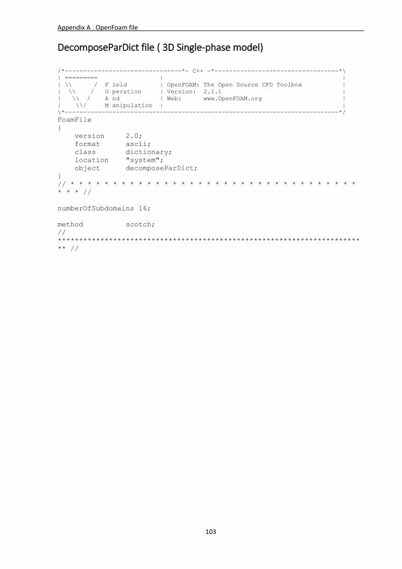
Appendix A . OpenFoam file
103
DecomposeParDict file ( 3D Single-phase model)
/*--------------------------------*- C++ -*----------------------------------*\
| ========= | |
| \\ / F ield | OpenFOAM: The Open Source CFD Toolbox |
| \\ / O peration | Version: 2.1.1 |
| \\ / A nd | Web: www.OpenFOAM.org |
| \\/ M anipulation | |
\*---------------------------------------------------------------------------*/
FoamFile
{
version 2.0;
format ascii;
class dictionary;
location "system";
object decomposeParDict;
}
// * * * * * * * * * * * * * * * * * * * * * * * * * * * * * * * * * *
* * * //
numberOfSubdomains 16;
method scotch;
//
***********************************************************************
** //

Appendix A . OpenFoam file
104
FvSchemes file ( 3D Single-phase model)
/*--------------------------------*- C++ -*----------------------------------*\
| ========= | |
| \\ / F ield | OpenFOAM: The Open Source CFD Toolbox |
| \\ / O peration | Version: 2.3.1 |
| \\ / A nd | Web: www.OpenFOAM.org |
| \\/ M anipulation | |
\*---------------------------------------------------------------------------*/
FoamFile
{
version 2.0;
format ascii;
class dictionary;
location "system";
object fvSchemes;
}
// * * * * * * * * * * * * * * * * * * * * * * * * * * * * * * * * * *
* * * //
ddtSchemes
{
default Euler;
}
gradSchemes
{
default Gauss linear;
}
divSchemes
{
default none;
div(phi,U) Gauss limitedLinearV 1;
div(phi,k) Gauss limitedLinear 1;
div(phi,omega) Gauss limitedLinear 1;
div(phi,R) Gauss limitedLinear 1;
div(R) Gauss linear;
div((nuEff*dev(T(grad(U))))) Gauss linear;
}
laplacianSchemes
{
default Gauss linear corrected;
}
interpolationSchemes
{
default linear;
}
snGradSchemes
{
default corrected;
}
fluxRequired
{
default no;
p ;
}
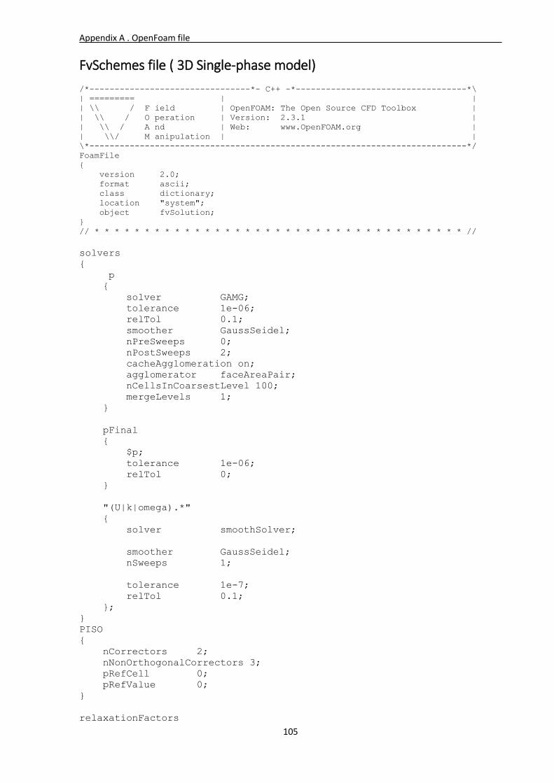
Appendix A . OpenFoam file
105
FvSchemes file ( 3D Single-phase model)
/*--------------------------------*- C++ -*----------------------------------*\
| ========= | |
| \\ / F ield | OpenFOAM: The Open Source CFD Toolbox |
| \\ / O peration | Version: 2.3.1 |
| \\ / A nd | Web: www.OpenFOAM.org |
| \\/ M anipulation | |
\*---------------------------------------------------------------------------*/
FoamFile
{
version 2.0;
format ascii;
class dictionary;
location "system";
object fvSolution;
}
// * * * * * * * * * * * * * * * * * * * * * * * * * * * * * * * * * * * * * //
solvers
{
p
{
solver GAMG;
tolerance 1e-06;
relTol 0.1;
smoother GaussSeidel;
nPreSweeps 0;
nPostSweeps 2;
cacheAgglomeration on;
agglomerator faceAreaPair;
nCellsInCoarsestLevel 100;
mergeLevels 1;
}
pFinal
{
$p;
tolerance 1e-06;
relTol 0;
}
"(U|k|omega).*"
{
solver smoothSolver;
smoother GaussSeidel;
nSweeps 1;
tolerance 1e-7;
relTol 0.1;
};
}
PISO
{
nCorrectors 2;
nNonOrthogonalCorrectors 3;
pRefCell 0;
pRefValue 0;
}
relaxationFactors
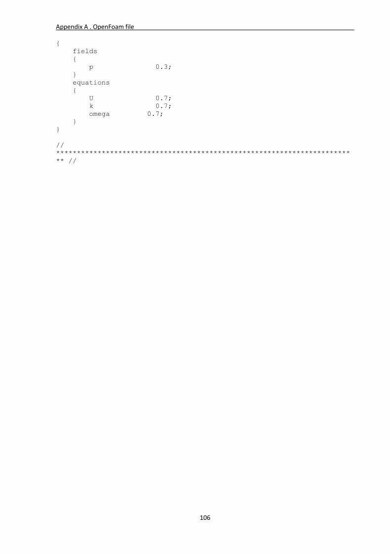
Appendix A . OpenFoam file
106
{
fields
{
p 0.3;
}
equations
{
U 0.7;
k 0.7;
omega 0.7;
}
}
//
***********************************************************************
** //
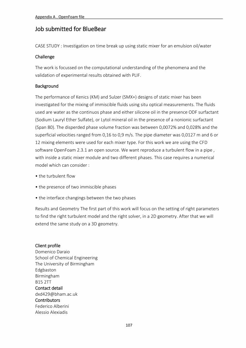
Appendix A . OpenFoam file
107
Job submitted for BlueBear
CASE STUDY : Investigation on time break up using static mixer for an emulsion oil/water
Challenge
The work is focussed on the computational understanding of the phenomena and the
validation of experimental results obtained with PLIF.
Background
The performance of Kenics (KM) and Sulzer (SMX+) designs of static mixer has been
investigated for the mixing of immiscible fluids using situ optical measurements. The fluids
used are water as the continuos phase and either silicone oil in the presence ODF surfactant
(Sodium Lauryl Ether Sulfate), or Lytol mineral oil in the presence of a nonionic surfactant
(Span 80). The disperded phase volume fraction was between 0,0072% and 0,028% and the
superficial velocities ranged from 0,16 to 0,9 m/s. The pipe diameter was 0,0127 m and 6 or
12 mixing elements were used for each mixer type. For this work we are using the CFD
software OpenFoam 2.3.1 an open source. We want reproduce a turbulent flow in a pipe ,
with inside a static mixer module and two different phases. This case requires a numerical
model which can consider :
• the turbulent flow
• the presence of two immiscible phases
• the interface changings between the two phases
Results and Geometry The first part of this work will focus on the setting of right parameters
to find the right turbulent model and the right solver, in a 2D geometry. After that we will
extend the same study on a 3D geometry.
Client profile Domenico Daraio School of Chemical Engineering The University of Birmingham Edgbaston Birmingham B15 2TT Contact detail [email protected] Contributors Federico Alberini Alessio Alexiadis
108
REFERENCES
Aveyard, R., et al. (2003). "Emulsions stabilised solely by colloidal particles." Advances in Colloid and Interface Science 100–102: 503-546. Barnes, H. A. (1994). "A selection of papers presented at the First World Congress on EmulsionsRheology of emulsions — a review." Colloids and Surfaces A: physicochemical and Engineering Aspects 91: 89-95. Briscoe, B. J., et al. (1999). "A review of immiscible fluid mixing." Advances in Colloid and Interface Science 81(1): 1-17. Ceylan, S., et al. (2003). "Estimation of the maximum stable drop sizes, coalescence frequencies and the size distributions in isotropic turbulent dispersions." Colloids and Surfaces A: Physicochemical and Engineering Aspects 212(2–3): 285-295. Chern, C.-S., et al. (1997). "Emulsion polymerization of styrene stabilized by mixed anionic and nonionic surfactants." Polymer 38(8): 1977-1984. Clark, M. M. (1988). "Drop breakup in a turbulent flow—I. Conceptual and modeling considerations." Chemical Engineering Science 43(3): 671-679. Das, P. K., et al. (2005). "Drop breakage model in static mixers at low and intermediate Reynolds number." Chemical Engineering Science 60(1): 231-238. Daub, A., et al. (2013). "Measurement of maximum stable drop size in aerated dilute liquid–liquid dispersions in stirred tanks." Chemical Engineering Science 104: 147-155. Eastwood, Craig Douglas, L. Armi, and J. C. Lasheras. "The breakup of immiscible fluids
in turbulent flows." Journal of Fluid Mechanics 502 (2004): 309-333.
Fernandez, P., et al. (2004). "Nano-emulsion formation by emulsion phase inversion." Colloids and Surfaces A: Physicochemical and Engineering Aspects 251(1–3): 53-58. Forte Giuseppe (2015). “Use of PLIF to investigate mixing of immiscible liquids in static mixer.” Thesis from University of Pisa Galinat, S., et al. (2005). "Drop break-up in turbulent pipe flow downstream of a restriction." Chemical Engineering Science 60(23): 6511-6528.
References
109
Ghanem, A., et al. (2014). "Static mixers: Mechanisms, applications, and characterization methods – A review." Chemical Engineering Research and Design 92(2): 205-228. Han, L., et al. (2011). "A theoretical model for droplet breakup in turbulent dispersions." Chemical Engineering Science 66(4): 766-776. Haursawa, F. and T. Mitsui (1975). "Stability of emulsions." Progress in Organic Coatings 3(2): 177-190. Hesketh, R. P., et al. (1991). "Bubble breakage in pipeline flow." Chemical Engineering Science 46(1): 1-9. Israelachvili, J. (1994). "The science and applications of emulsions — an overview." Colloids and Surfaces A: Physicochemical and Engineering Aspects 91: 1-8. Ivanov, I. B. and P. A. Kralchevsky (1997). "Stability of emulsions under equilibrium and dynamic conditions." Colloids and Surfaces A: Physicochemical and Engineering Aspects 128(1–3): 155-175. Jafari, S. M., et al. (2008). "Re-coalescence of emulsion droplets during high-energy emulsification." Food Hydrocolloids 22(7): 1191-1202. Kékesi, T., et al. "Drop deformation and breakup in flows with shear." Chemical Engineering Science. Kumar, S., et al. (1991). "Alternative mechanisms of drop breakage in stirred vessels." Chemical Engineering Science 46(10): 2483-2489. Lazaridis, N., et al. (1999). "Steric stabilization in emulsion polymerization using oligomeric nonionic surfactants." Chemical Engineering Science 54(15–16): 3251-3261. Lee, C. H. and R. D. Reitz (2000). "An experimental study of the effect of gas density on the distortion and breakup mechanism of drops in high speed gas stream." International Journal of Multiphase Flow 26(2): 229-244. Lemenand, T., et al. (2003). "Droplets formation in turbulent mixing of two immiscible fluids in a new type of static mixer." International Journal of Multiphase Flow 29(5): 813-840. Lemenand, T., et al. (2003). "Droplets formation in turbulent mixing of two immiscible fluids in a new type of static mixer." International Journal of Multiphase Flow 29(5): 813-840.
References
110
Liu, Z. and R. D. Reitz (1997). "An analysis of the distortion and breakup mechanisms of high speed liquid drops." International Journal of Multiphase Flow 23(4): 631-650. Luo, Hean, and Hallvard F. Svendsen. "Theoretical model for drop and bubble breakup
in turbulent dispersions." AIChE Journal-American Institute of Chemical Engineers 42.5
(1996): 1225-1233.
Mäkelä, J. S., et al. (2008). "Properties of preliminary breakdown processes in Scandinavian lightning." Journal of Atmospheric and Solar-Terrestrial Physics 70(16): 2041-2052. Meijer, H. E. H., et al. (2012). "On the performance of static mixers: A quantitative comparison." Progress in Polymer Science 37(10): 1333-1349. Nachtigall, S., et al. "Analysis of drop deformation dynamics in turbulent flow." Chinese Journal of Chemical Engineering. Napper, D. H. (1977). "Steric stabilization." Journal of Colloid and Interface Science 58(2): 390-407. Napper, D. H. and A. Netschey (1971). "Studies of the steric stabilization of colloidal particles." Journal of Colloid and Interface Science 37(3): 528-535. Nazir, A., et al. (2013). "Droplet break-up mechanism in premix emulsification using packed beds." Chemical Engineering Science 92: 190-197. Nere, Nandkishor K., Ashwin W. Patwardhan, and Jyeshtharaj B. Joshi. "Liquid-phase
mixing in stirred vessels: turbulent flow regime." Industrial & engineering chemistry
research 42.12 (2003): 2661-2698.
Paglianti, A. and G. Montante (2013). "A mechanistic model for pressure drops in corrugated plates static mixers." Chemical Engineering Science 97: 376-384. Pal, R. (2000). "Shear Viscosity Behavior of Emulsions of Two Immiscible Liquids." Journal of Colloid and Interface Science 225(2): 359-366. Peng, S. J. and R. A. Williams (1998). "Controlled Production of Emulsions Using a Crossflow Membrane: Part I: Droplet Formation from a Single Pore." Chemical Engineering Research and Design 76(8): 894-901. Sahu, A. K., et al. (1999). "CFD modelling and mixing in stirred tanks." Chemical Engineering Science 54(13–14): 2285-2293.
References
111
Schuch, A., et al. (2014). "Production of W/O/W double emulsions. Part I: Visual observation of deformation and breakup of double emulsion drops and coalescence of the inner droplets." Colloids and Surfaces A: Physicochemical and Engineering Aspects 461: 336-343. Tadros, T. (2004). "Application of rheology for assessment and prediction of the long-term physical stability of emulsions." Advances in Colloid and Interface Science 108–109: 227-258. Tadros, T. F. (1994). "Fundamental principles of emulsion rheology and their applications." Colloids and Surfaces A: Physicochemical and Engineering Aspects 91: 39-55. Thakur, R. K., et al. (2003). "Static Mixers in the Process Industries—A Review." Chemical Engineering Research and Design 81(7): 787-826. Tidhar, M., et al. (1986). "Characteristics of a motionless mixer for dispersion of immiscible fluids—II. Phase inversion of liquid-liquid systems." Chemical Engineering Science 41(3): 457-462. Van den Akker, H. E. A. (2006). The Details of Turbulent Mixing Process and their Simulation. Advances in Chemical Engineering. B. M. Guy, Academic Press. Volume 31: 151-229. Walstra, P. (1993). "Principles of emulsion formation." Chemical Engineering Science 48(2): 333-349. Zhang, L., et al. (2015). "A study of mixing performance of polyacrylamide solutions in a new-type static mixer combination." Chemical Engineering and Processing: Process Intensification 88: 19-28. Hirschberg, S., et al. (2009). "An improvement of the Sulzer SMX™ static mixer significantly reducing the pressure drop." Chemical Engineering Research and Design 87(4): 524-532. Ascanio, G., et al. (2004). "Measurement of Power Consumption in Stirred Vessels—A Review." Chemical Engineering Research and Design 82(9): 1282-1290. Kumaresan, T. and J. B. Joshi (2006). "Effect of impeller design on the flow pattern and mixing in stirred tanks." Chemical Engineering Journal 115(3): 173-193. Uppal, A., et al. (1974). "On the dynamic behavior of continuous stirred tank reactors." Chemical Engineering Science 29(4): 967-985.
References
112
Pacek, A. W., et al. (1998). "On the Sauter mean diameter and size distributions in turbulent liquid/liquid dispersions in a stirred vessel." Chemical Engineering Science 53(11): 2005-2011. Kumar, R. "Dispersion in stirred vessels." Journal of the Indian Institute of Science 72.3
(2013): 235. Freudig, B., et al. (1999). "Dispersion of powders in liquids in a stirred vessel." Chemical Engineering and Processing: Process Intensification 38(4–6): 525-532. Lagisetty, J. S., et al. (1986). "Breakage of viscous and non-Newtonian drops in stirred dispersions." Chemical Engineering Science 41(1): 65-72. Coroneo, M., et al. (2011). "CFD prediction of fluid flow and mixing in stirred tanks: Numerical issues about the RANS simulations." Computers & Chemical Engineering 35(10): 1959-1968. Hobbs, D. M. and F. J. Muzzio (1997). "The Kenics static mixer: a three-dimensional chaotic flow." Chemical Engineering Journal 67(3): 153-166. Byrde, O. and M. L. Sawley (1999). "Optimization of a Kenics static mixer for non-creeping flow conditions." Chemical Engineering Journal 72(2): 163-169. Martínez, J., et al. (2015). "Influence of spatial discretization schemes on accuracy of explicit LES: Canonical problems to engine-like geometries." Computers & Fluids 117: 62-78. Jalali, A., et al. (2014). "Accuracy analysis of unstructured finite volume discretization schemes for diffusive fluxes." Computers & Fluids 101: 220-232.

113
Ringraziamenti
Sono arrivato al termine di un lungo percorso iniziato ormai 6 anni fa, pieno di sacrifici, lunghe
giornate passate a studiare e di progetti sempre in attesa di essere consegnati. Ma, allo stesso
tempo questi sono stati anni pieni di gioie e di soddisfazioni, gli anni della maggiore libertà e
delle responsabilità, gli anni in cui ho conosciuto tanti nuovi amici con cui spero di continuare
a condividere preziosi momenti. Questa tesi poi è il frutto di una meravigliosa esperienza
all’estero durata 6 mesi, in Inghilterra, all’ università di Birmingham. Ho sempre desiderato fare
un esperienza di questo tipo ma, non ho mai avuto davvero la forza di partire, il coraggio di
andare in un posto dove non sarei stato in grado di comunicare. Alla fine le circostanze sono
state tali da non poter dire di no, sono partito e tornato più determinato di prima, più
consapevole dei miei mezzi e più ricco dentro. Infatti, in questi mesi spesi a Birmingham ho
conosciuto molti ragazzi unici nella loro semplicità, provenienti da tutto il mondo che hanno
saputo condividere con me le loro esperienze, le loro aspirazioni e anche le loro passioni.
Questa stupenda occasione di crescita mi è stata data dalla prof. dell’università di Pisa
Elisabetta Brunazzi che non smetterò mai di ringraziare e dall’Ingegnere Federico Alberini che
mi ha accolto nel suo ufficio a braccia aperte. Federico mi ha presentato tutti, mi ha sostenuto
in tutto il mio lavoro di tesi e si è rivelato un valido collega e ancor più importante un amico
sincero pronto a mettere in secondo piano anche il proprio lavoro per aiutarmi. Grazie Fede,
non avrei mai potuto fare quello che ho fatto senza di te.
Chi però mi ha davvero portato fin qui, chi mi ha indirizzato sempre nel seguire le miei passioni
sono i miei stupendi genitori, che insieme alle mie sorelle sono sempre state lì a fare il tifo per
me. Papà, mamma gran parte di quello che ho imparato nella vita lo devo a voi e adesso non
trovo nemmeno le parole giuste per ringraziarvi, ma sono sicuro che quando leggerete queste
righe capirete tutto.
E’ arrivato il momento di ringraziare la mia metà, la donna che ha sopportato tutte le mie
discussioni da Ingegnere, che mi ha dato la serenità per andare avanti e mi è stata accanto. Tu
che mi sei stata vicina anche quando eravamo lontani, passando un’intera estate con me in
Inghilterra. Grazie Erica, grazie amore.
Infine, ma non per importanza, ringrazio tutti gli amici con cui ho avuto la fortuna di vivere qui
a Pisa: Gianluca l’amico di una vita sempre lì, ovunque io fossi, Maurizio collega e fratello allo
stesso tempo (quante ne abbiamo passate insieme), Sabino giocatore incallito di calcetto,
Matteo, ragazzo davvero generoso, Manuele il perfezionista, Calogero e tutti gli altri. Tutti voi
avete reso ogni mio giorno più leggero, nonostante lo studio e i problemi della via quotidiana.