U.P.B. Sci. Bull., Series D, Vol. 75, Iss. 4, 2013 ISSN 1454-2358

NUMERICAL STUDY OF COMPRESSIBLE FLOW PAST A REENTRY VEHICLE NOSE

Bianca SZASZ1

In this paper, a numerical solution of compressible flow past a reentry vehicle nose is presented. The nose will be approximated with a circular shape for simplicity and the flow will be considered at supersonic and hypersonic speeds. Ansys Fluent software has been used and the objective of this work is to study the limits of Fluent capabilities to simulate the flow at high-speed by comparing the results with others similar in literature, with theoretical and experimental results, but also by comparing the results using three different methods for computing the specific heat at constant pressure.

Keywords: high-speed flow, numerical simulations, Ansys Fluent

1. Introduction

The high-speed flow over a reentry vehicle is one of the most studied problems in fluid dynamics and especially regarding the case of a blunt body like the reentry capsule from Apollo program. The particular shape of the reentry body would slow down the vehicle during atmospheric reentry. When a reentry body, like the reentry capsule, traveled at supersonic speed, a bow shock would form and it would significantly increases the drag experienced by the vehicle, thus slowing it down [1].

For simulating the flow around the vehicle nose, a CFD-software like Ansys Fluent can be used. However, Ansys Fluent presents a series of limitations like the carbuncle phenomenon (due to Riemann-Roe solver). Consequently, the results were compared to the case of Rotated-Hybrid Riemann solver [1].

Also, as a flaw inherent to the cases of high-speed flows, it is difficult to compute appropriately the specific heat at high temperatures. In this paper, three different methods have been used for computing the specific heat at constant pressure: one using a constant specific heat, one using a temperature function of piecewise-polynomial available in Ansys Fluent and one using a constant specific heat, calculated for the average temperature after the shock, using a function based on NASA coefficients [2].

1 Ph.D student, Faculty of Aerospace Engineering, University POLITEHNICA of Bucharest, e-mail: Bianca.Szasz@yahoo.com

4 Bianca Szasz

2. Methods

The Euler model has been used for simulating the flow around the nose. The Euler equations are a system of non-linear hyperbolic conservation laws that govern the dynamics of compressible flows. The effects of body forces, viscous stresses and heat flux are neglected. The Euler equations are based on the conservation of mass, momentum and energy and they are a coupled system of nonlinear partial differential equations [1]. Also, because the flow is at high-speeds, the inviscid model has been used and the fluid is considered as an ideal gas. The Mach numbers were set to 2, 3, 4, 5, 6, and respectively 8. Regarding the input parameters, they can be seen in Table 1.

Table 1 Free-stream Values

Free-stream Density ( ∞ρ ) 1.225 [kg/ 3m ]

Free-stream Static Temperature ( ∞T ) 288 [°K]

Free-stream Mach Number ( ∞M ) 2, 3, 4, 5, 6, 8

Gamma (γ ) 1.4 Gas Constant (R) 287 [J/ )( Kkg °⋅ ]

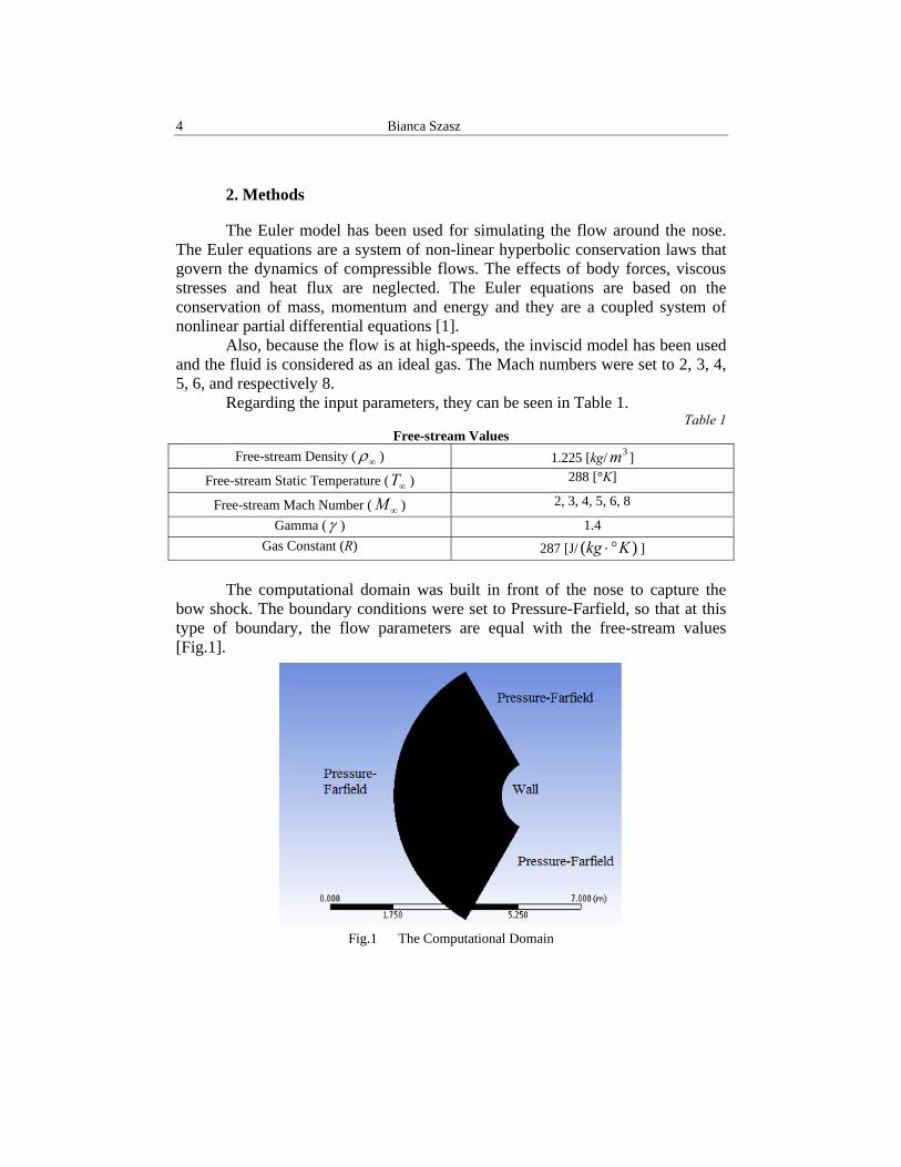
The computational domain was built in front of the nose to capture the bow shock. The boundary conditions were set to Pressure-Farfield, so that at this type of boundary, the flow parameters are equal with the free-stream values [Fig.1].

Fig.1 The Computational Domain

Numerical study of compressible flow past a reentry vehicle nose 5

The grid has the dimensions showed in Table 2. Table 2

Grid dimensions Faces Cells Nodes 70780 35200 35581

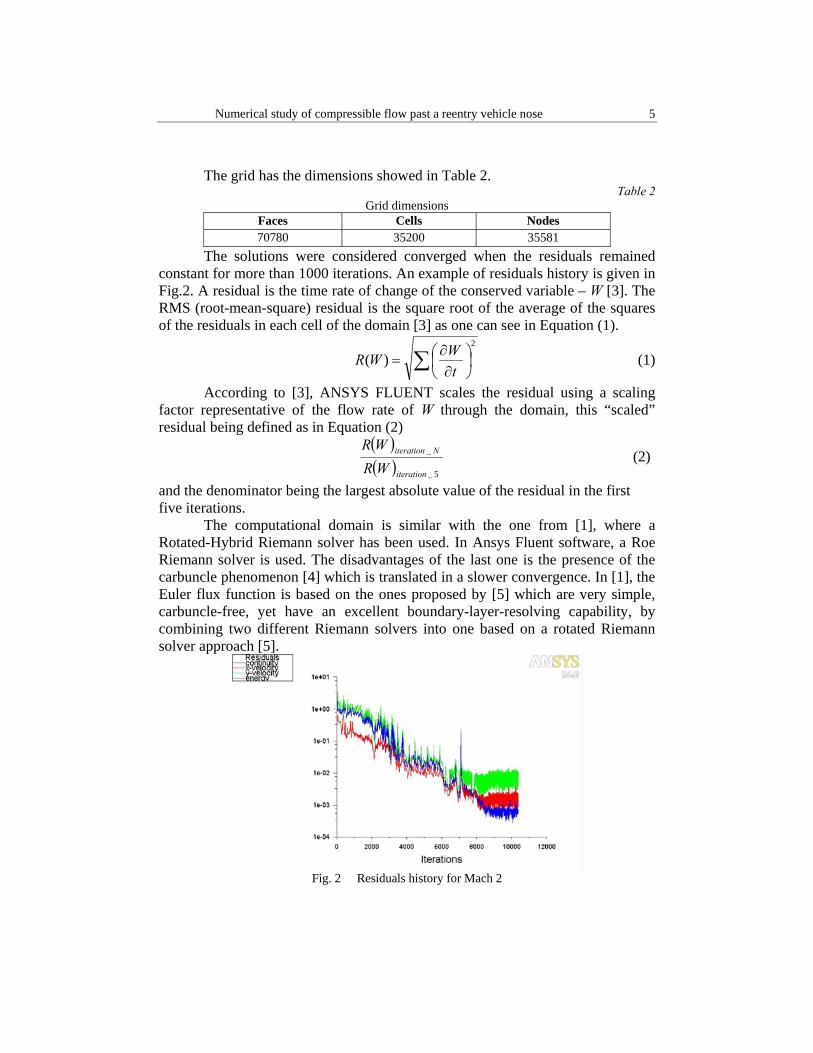
The solutions were considered converged when the residuals remained constant for more than 1000 iterations. An example of residuals history is given in Fig.2. A residual is the time rate of change of the conserved variable – W [3]. The RMS (root-mean-square) residual is the square root of the average of the squares of the residuals in each cell of the domain [3] as one can see in Equation (1).

∑ ⎟⎠⎞

⎜⎝⎛∂∂

=2

)(t

WWR (1)

According to [3], ANSYS FLUENT scales the residual using a scaling factor representative of the flow rate of W through the domain, this “scaled” residual being defined as in Equation (2)

( )( ) 5_

_

iteration

Niteration

WRWR

(2)

and the denominator being the largest absolute value of the residual in the first five iterations.

The computational domain is similar with the one from [1], where a Rotated-Hybrid Riemann solver has been used. In Ansys Fluent software, a Roe Riemann solver is used. The disadvantages of the last one is the presence of the carbuncle phenomenon [4] which is translated in a slower convergence. In [1], the Euler flux function is based on the ones proposed by [5] which are very simple, carbuncle-free, yet have an excellent boundary-layer-resolving capability, by combining two different Riemann solvers into one based on a rotated Riemann solver approach [5].

Fig. 2 Residuals history for Mach 2

6 Bianca Szasz

One of the most important thermodynamic property is the specific heat ratio, a parameter which can be considered constant only at low temperatures. For high temperatures, a temperature function should be applied.

For computing the specific heat at Mach 2, three different methods have been used: one with a constant specific heat of 1006.43 )/( KkgJ °⋅ , one using a constant specific heat (1023 )/( KkgJ °⋅ ), calculated for the average temperature (465°K) after the shock, using a caloric capacity function based on NASA Glenn coefficients [2] and one with a piecewise-polynomial function of temperature (Eq.2) with Ansys coefficients, from Ansys Fluent database for air. The first two methods have been used for Mach 8 too. The caloric capacity function is written as a power function (Eq.3).

∑=

−−=n

j

jj

vcF

1

3)( θαθθ (3)

where v, j are convenient natural numbers [2] ;3=v 7=j ,

and 1000T=θ , a non-dimensional parameter. In Ansys, there are several possible ways to compute the specific heat at

constant pressure beside setting it at a constant value: implementing a piecewise-linear function, a piecewise-polynomial function, a polynomial function, a user-defined function or implementing a kinetic theory method. In this paper, the piecewise-polynomial function has been used 7

76

65

54

43

32

210)( TATATATATATATAATcp +++++++= , (4) where T is defined for two intervals:

2max,2min, TTT <≤

1max,1min, TTT <≤ 1min,T is set to 100°K, 2min,1max, TT = to 1000°K, 2max,T to 3000°K. The coefficients ( 76543210 ,,,,,,, AAAAAAAA ) have been taken from Fluent database for air [3].

3. Results

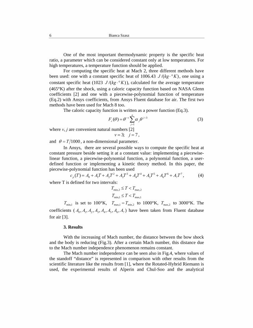
With the increasing of Mach number, the distance between the bow shock and the body is reducing (Fig.3). After a certain Mach number, this distance due to the Mach number independence phenomenon remains constant.

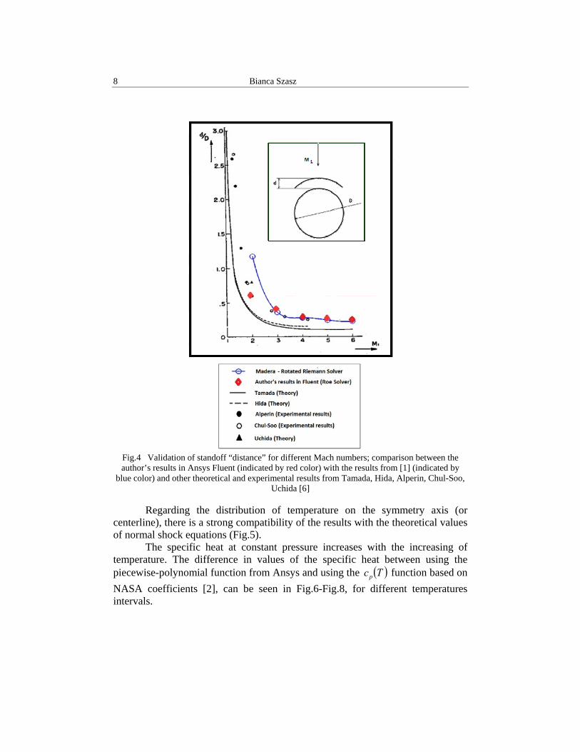
The Mach number independence can be seen also in Fig.4, where values of the standoff “distance” is represented in comparison with other results from the scientific literature like the results from [1], where the Rotated-Hybrid Riemann is used, the experimental results of Alperin and Chul-Soo and the analytical

Numerical study of compressible flow past a reentry vehicle nose 7

approximations of Tamada, Hida and Uchida [6]. The comparison shows a very good compatibility between author’s results and the analytical approximations of Tamada, Hida and Uchida. Below Mach 3, there is a relative big difference between these results and the results of the Rotated-Hybrid Riemann solver from [1].

(a) (b)

(c) (d)

Fig.3. Pressure contours for: (a) Mach 2; (b) Mach 4; (c) Mach 6; (d) Mach 8; Fluent results obtained by the author

8 Bianca Szasz

Fig.4 Validation of standoff “distance” for different Mach numbers; comparison between the author’s results in Ansys Fluent (indicated by red color) with the results from [1] (indicated by

blue color) and other theoretical and experimental results from Tamada, Hida, Alperin, Chul-Soo, Uchida [6]

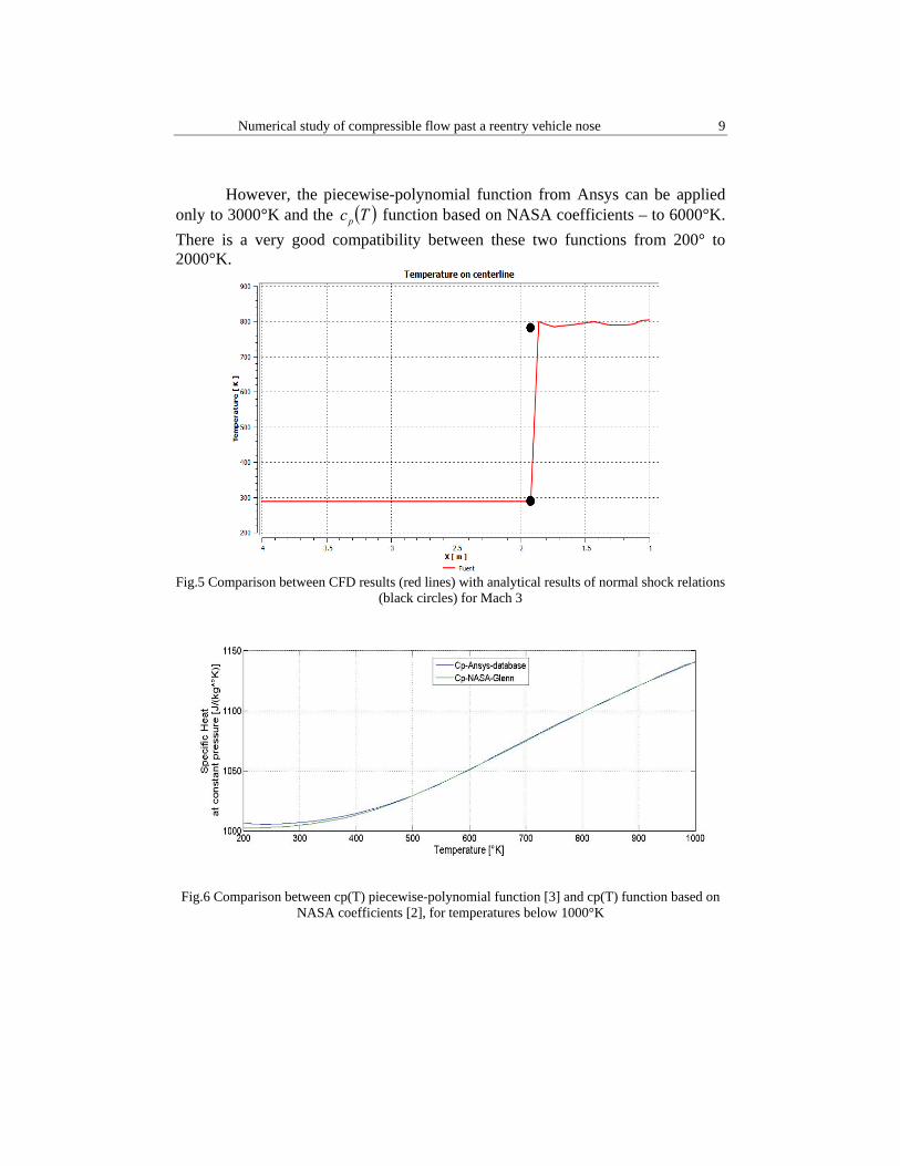
Regarding the distribution of temperature on the symmetry axis (or

centerline), there is a strong compatibility of the results with the theoretical values of normal shock equations (Fig.5).

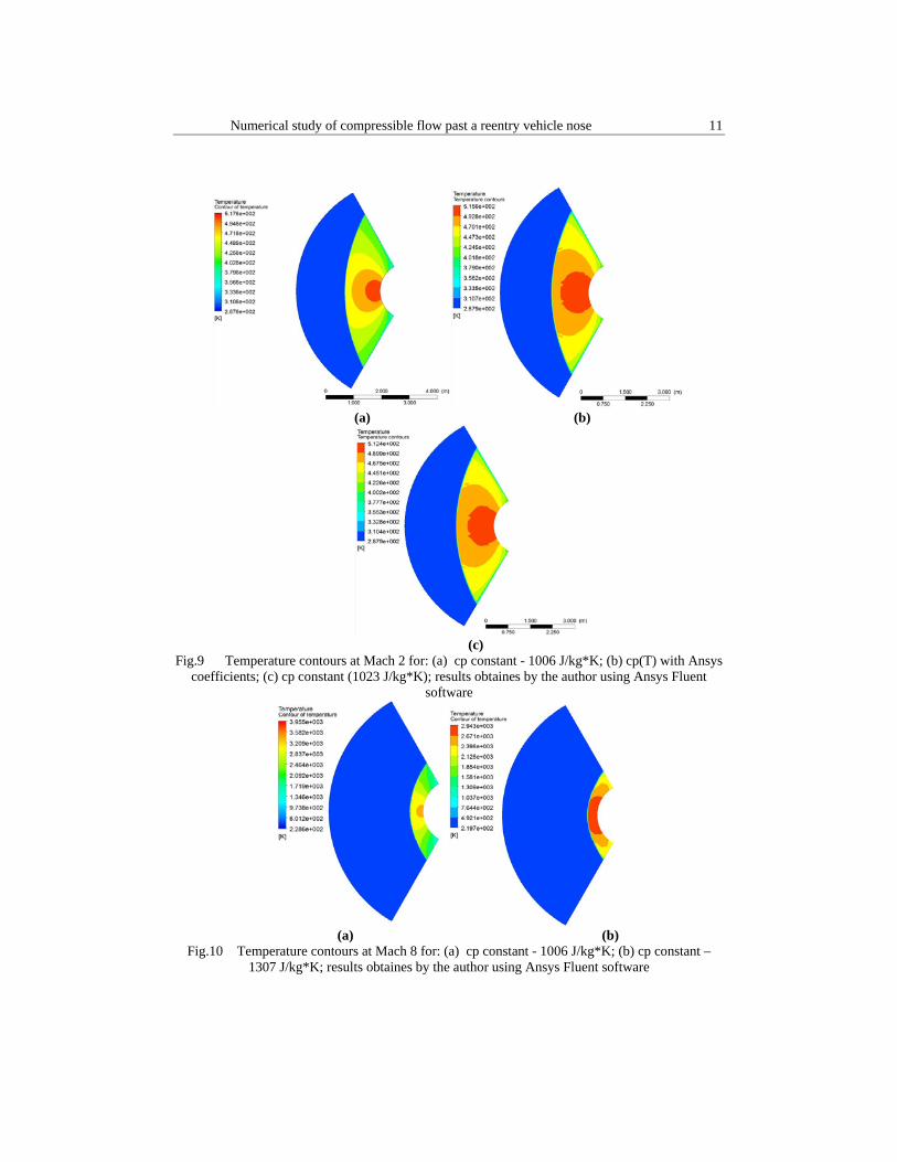
The specific heat at constant pressure increases with the increasing of temperature. The difference in values of the specific heat between using the piecewise-polynomial function from Ansys and using the ( )Tcp function based on NASA coefficients [2], can be seen in Fig.6-Fig.8, for different temperatures intervals.

Numerical study of compressible flow past a reentry vehicle nose 9

However, the piecewise-polynomial function from Ansys can be applied only to 3000°K and the ( )Tcp function based on NASA coefficients – to 6000°K. There is a very good compatibility between these two functions from 200° to 2000°K.

Fig.5 Comparison between CFD results (red lines) with analytical results of normal shock relations

(black circles) for Mach 3

Fig.6 Comparison between cp(T) piecewise-polynomial function [3] and cp(T) function based on

NASA coefficients [2], for temperatures below 1000°K

10 Bianca Szasz

Fig.7 Comparison between cp(T) piecewise-polynomial function [3] and cp(T) function based on

NASA coefficients [2], for temperatures between 1000°K and 3000°K

Fig.8 cp(T) function based on NASA coefficients [2], for temperatures between 1000°K and

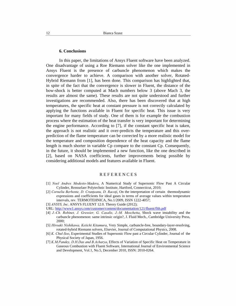
6000°K For small Mach numbers like 2, where the average after-shock temperature is around 450°K, there is almost no difference in temperature contours between the two methods of piecewise-polynomial function from Ansys and the function based on NASA coefficients [2] (Fig.9). However, at high Mach number as 8, the temperature is so high (above 3000°K) that the piecewise-polynomial function from Ansys can’t be applied, because this function works only between 0° and 3000°K. Also, there can be noted that there is a difference of about 1000°K between the temperatures after the shock when using a constant specific heat of 1006 J/(kg*K) and when using a different value for the specific heat, calculated with the ( )Tcp function, based on NASA coefficients [2], for the stimated average temperature after the shock (Fig.10).

Numerical study of compressible flow past a reentry vehicle nose 11

(a) (b)

(c)

Fig.9 Temperature contours at Mach 2 for: (a) cp constant - 1006 J/kg*K; (b) cp(T) with Ansys coefficients; (c) cp constant (1023 J/kg*K); results obtaines by the author using Ansys Fluent

software

(a) (b)

Fig.10 Temperature contours at Mach 8 for: (a) cp constant - 1006 J/kg*K; (b) cp constant – 1307 J/kg*K; results obtaines by the author using Ansys Fluent software

12 Bianca Szasz

6. Conclusions

In this paper, the limitations of Ansys Fluent software have been analyzed. One disadvantage of using a Roe Riemann solver like the one implemented in Ansys Fluent is the presence of carbuncle phenomenon which makes the convergence harder to achieve. A comparison with another solver, Rotated-Hybrid Riemann from [1], has been done. This comparison has highlighted that, in spite of the fact that the convergence is slower in Fluent, the distance of the bow-shock is better computed at Mach numbers below 3 (above Mach 3, the results are almost the same). These results are not quite understood and further investigations are recommended. Also, there has been discovered that at high temperatures, the specific heat at constant pressure is not correctly calculated by applying the functions available in Fluent for specific heat. This issue is very important for many fields of study. One of them is for example the combustion process where the estimation of the heat transfer is very important for determining the engine performance. According to [7], if the constant specific heat is taken, the approach is not realistic and it over-predicts the temperature and this over-prediction of the flame temperature can be corrected by a more realistic model for the temperature and composition dependence of the heat capacity and the flame length is much shorter in variable Cp compare to the constant Cp. Consequently, in the future, it should be implemented a new function, like the one described in [2], based on NASA coefficients, further improvements being possible by considering additional models and features available in Fluent.

R E F E R E N C E S

[1] Noel Andres Modesto-Madera, A Numerical Study of Supersonic Flow Past A Circular Cylinder, Rensselaer Polytechnic Institute, Hartford, Connecticut, 2010;

[2] Corneliu Berbente, D. Crunţeanu, D. Racoţi, On the interpretation of certain thermodynamic expressions and coefficients for ideal gases in terms of average values within temperature intervals, rev. TERMOTEHNICA, No.1/2009, ISSN 1222-4057;

[3] ANSYS, Inc, ANSYS FLUENT 12.0. Theory Guide (2012); URL: http://www1.ansys.com/customer/content/documentation/121/fluent/flth.pdf [4] J.-Ch. Robinet, J. Gressier, G. Casalis, J.-M. Moschetta, Shock wave instability and the

carbuncle phenomenon: same intrinsic origin?, J. Fluid Mech., Cambridge University Press, 2000;

[5] Hiroaki Nishikawa, Keiichi Kitamura, Very Simple, carbuncle-free, boundary-layer-resolving, rotated-hybrid Riemann solvers, Elsevier, Journal of Computational Physics, 2008.

[6] K. Chul-Soo, Experimental Studies of Supersonic Flow past a Circular Cylinder, Journal of the Physical Society of Japan, 1956.

[7] K.M.Pandey, D.H.Das and B.Acharya, Effects of Variation of Specific Heat on Temperature in Gaseous Combustion with Fluent Software, International Journal of Environmental Science and Development, Vol.1, No.5, December 2010, ISSN: 2010-0264.