numerical simulations of bile flow in realistic image

Biotechnology Center

Dresden University of Technology

Master’s Thesis

Numerical Simulations of BileFlow in Realistic Image-Derived

Bile Canalicular Geometries

Author:

Ali Ghaemi

First Supervisor:

Ivo Sbalzarini

Second Supervisor:

Jochen Guck

A thesis submitted in fulfilment of the requirements

for the degree of Master of Science

in the

Dr. Sbalzarini’s Lab - MOSAIC Group

Max Planck Institute of Molecular Cell Biology and Genetics

November 2013

http://mosaic.mpi-cbg.de/?q=people/members

http://www.mpi-cbg.de/de/research/research-groups/ivo-sbalzarini/group-leader.html

http://www.biotec.tu-dresden.de/research/guck.html

http://mosaic.mpi-cbg.de/

Declaration of Authorship

I, Ali Ghaemi, declare that this thesis titled, Numerical Simulations of Bile Flow

in Realistic Image-Derived Bile Canalicular Geometries and the work presented

in it are my own. I also confirm that:

� Where I have consulted the published or unpublished work of the others,

this is always clearly attributed.

� Where I have quoted from the work of the others, the source is always given.

� All the free source softwares used in this project are mentioned and the com-

mercial softwares were all used under the license purchased by Max Planck

Institute of Molecular Cell Biology and Genetics

� I have acknowledged all the main sources of help.

Signed:

Date:

ii

iii

AbstractThe liver plays a key role in the metabolism of nutrients and xenobiotics, as

well as in detoxification.Tight junctions between liver cells (Hepatocytes) apical

membranes form a three-dimensional (3D) narrow belt between adjacent cells,

which gives rise to the bile canalicular (BCa) network, that is essential for bile

secretion and liver function.

In this project, Canalicular geometries were reconstructed separately from 2D

TEM and 3D SBF-SEM data in order to account for the internal micro-structures

of the BCa. Finite-volume based computational fluid dynamics simulations of

the 3D flow in realistic bile canaliculi were performed in order to obtain flow

parameters. The results were compared with the flow in a smooth pipe with

cylindrical cross-sectional area in order to calculate an equivalent diameter on the

basis of Hagen–Poiseuille equation.

Acknowledgements

First and foremost, I would like to express my special thanks to my first supervisor

Dr. I. Sbalzarini for his continuous support through this project. I also thank my

second supervisor Prof. J. Guck.

The goals of this interdisciplinary research wouldn’t be achieved without the in-

valuable help and support from the the other experts and the individuals from

different disciplines. Then I would like to give gratitude to: Dr. J.M. Verba-

vatz, the leader of the electron microscopy facility in MPI-CBG, for providing the

SBF-SEM images and the very helpful discussions on microscopy setups and the

analysis of the images, Prof. Y.L. Kalaidzidis and his colleagues that helped me

with the processing and the analysis of SBF-SEM and TEM images, Prof. M.

Zerial and the members of his lab for helpful discussions on biological aspects of

the project, U.Guenther, the guest student in MOSAIC group for his help with

preparing the videos of 3D structures and my friend Y. Bodrov for his help with

styling the text.

iv

Contents

Declaration of Authorship ii

Abstract iii

Acknowledgements iv

Contents v

List of Figures ix

List of Tables xi

Abbreviations xiii

1 Introduction 1

1.1 Bile Canalicular Network . . . . . . . . . . . . . . . . . . . . . . . . 1

1.2 Microscopy . . . . . . . . . . . . . . . . . . . . . . . . . . . . . . . 4

1.2.1 Serial block-face scanning electron microscopy (SBF-SEM) . 4

1.3 Image Based Computational Fluid Dynamics Simulations of theBile Flow . . . . . . . . . . . . . . . . . . . . . . . . . . . . . . . . 5

1.3.1 Computational Fluid Dynamics . . . . . . . . . . . . . . . . 6

Mathematical Model . . . . . . . . . . . . . . . . . . 6

Discretization Method . . . . . . . . . . . . . . . . . 6

Finite Volume Method . . . . . . . . . . . . . . . . . 6

Coordinate and Basis Vector Systems . . . . . . . . . 7

Numerical Grids . . . . . . . . . . . . . . . . . . . . . 7

Finite Approximations . . . . . . . . . . . . . . . . . 7

Solution Method . . . . . . . . . . . . . . . . . . . . . 8

Convergence Criteria . . . . . . . . . . . . . . . . . . 8

2 Methods 9

2.1 Microscopy . . . . . . . . . . . . . . . . . . . . . . . . . . . . . . . 9

2.1.1 Sample Preparation . . . . . . . . . . . . . . . . . . . . . . . 9

2.1.2 SBF-SEM . . . . . . . . . . . . . . . . . . . . . . . . . . . . 9

2.2 Image Processing . . . . . . . . . . . . . . . . . . . . . . . . . . . . 10

v

Contents vi

2.3 3D Reconstruction and Mesh Generation . . . . . . . . . . . . . . . 10

2.3.1 Selecting the Region of Interest . . . . . . . . . . . . . . . . 10

2.4 Computational Fluid Mechanics Simulations . . . . . . . . . . . . . 11


Discretization Method . . . . . . . . . . . . . . . . . 11

Coordinate and Basis Vector Systems . . . . . . . . . 11

Numerical Grids . . . . . . . . . . . . . . . . . . . . . 11

Finite Approximations . . . . . . . . . . . . . . . . . 12

Solution Method . . . . . . . . . . . . . . . . . . . . . 12

Convergence Criteria . . . . . . . . . . . . . . . . . . 12

Visualizing the Results . . . . . . . . . . . . . . . . . 12

Writing and Styling . . . . . . . . . . . . . . . . . . . 12

3 Results 13

3.1 Image Processing . . . . . . . . . . . . . . . . . . . . . . . . . . . . 13

3.2 Reconstruction . . . . . . . . . . . . . . . . . . . . . . . . . . . . . 15

3.2.1 Initial Reconstruction of Bile Canaliculus . . . . . . . . . . . 15

3.2.2 Three-dimensional Reconstruction of Bile Canaliculus . . . . 16

3.3 Mesh Generation . . . . . . . . . . . . . . . . . . . . . . . . . . . . 19

3.4 Computational Fluid Dynamics Simulations . . . . . . . . . . . . . 20

3.4.1 CFD Simulations of Bile Flow in the Bile Canaliculus Re-constructed from TEM data . . . . . . . . . . . . . . . . . . 20

3.4.1.1 Components of the Numerical Solution . . . . . . . 20


Boundary Conditions . . . . . . . . . . . . . . . . . . 20

Numerical Grid . . . . . . . . . . . . . . . . . . . . . 21

3.4.1.2 Studying the Numerical Solution . . . . . . . . . . 21

Stability . . . . . . . . . . . . . . . . . . . . . . . . . 21

Convergence . . . . . . . . . . . . . . . . . . . . . . . 22

Studying the Flow . . . . . . . . . . . . . . . . . . . . 22

Visualization of the Numerical Solution . . . . . . . . 23

3.4.2 Computational Fluid Dynamics Simulations of 3D Bile Canalicu-lus . . . . . . . . . . . . . . . . . . . . . . . . . . . . . . . . 25

3.4.2.1 Components of the Numerical Solution . . . . . . . 25



Numerical Grid . . . . . . . . . . . . . . . . . . . . . 26

3.4.2.2 Study of the Numerical Solution . . . . . . . . . . 26

Stability . . . . . . . . . . . . . . . . . . . . . . . . . 26

Convergence . . . . . . . . . . . . . . . . . . . . . . . 27

Study of The Flow . . . . . . . . . . . . . . . . . . . 27


4 Discussion 31

4.1 Simulations of The Bile Flow in Bile Canaliculi . . . . . . . . . . . 31

Contents vii

4.2 Equivalent Diameter . . . . . . . . . . . . . . . . . . . . . . . . . . 32

4.3 Summary and Conclusion . . . . . . . . . . . . . . . . . . . . . . . 33

4.4 Future Prospects . . . . . . . . . . . . . . . . . . . . . . . . . . . . 34

A Verification of The Solver 37

A.1 Simulating the Flow of Liquid Waterin Simple Geometries . . . . . . . . . . . . . . . . . . . . . . . . . . 37

A.1.1 The Flow Between Two Parallel Plates . . . . . . . . . . . . 37

A.1.1.1 Components of the Numerical Solution . . . . . . . 37



Numerical Grid . . . . . . . . . . . . . . . . . . . . . 38

A.1.1.2 Study of the Numerical solution . . . . . . . . . . . 38

Convergence and Accuracy . . . . . . . . . . . . . . . 38


A.1.2 Simulating Hagen–Poiseuille Flow . . . . . . . . . . . . . . . 40

A.1.2.1 Components of the Numerical Solution . . . . . . . 40



Numerical Grid . . . . . . . . . . . . . . . . . . . . . 40

A.1.2.2 Study of the numerical solution . . . . . . . . . . . 40

Convergence and Accuracy . . . . . . . . . . . . . . . 40

Visualization of the numerical Solution . . . . . . . . 41

B Serial Block-Face Scanning Electron Microscopy Setup 43

Bibliography 47

List of Figures

1.1 Schematic view of BCas(shown as B.C in this picture) formed be-tween two adjacent hepatocaytes, surrounded by actin micro-filaments(m.f)and sealed by tight junctions(t.j). (n) is the nucleus[2] . . . . . . . 2

1.2 TEM image of BCa microvilli (pointed to by arrow) [provided byJerome Gilleron in Prof. Zerial’s lab] . . . . . . . . . . . . . . . . . 2

1.3 confocal microscopy image of canalicular web. provided by YannisKalaidzidis and Hidenori Nonaka in Prof. Zerial’s lab. SEM imageof bile canaliculie revealing the 3D arrangement of BCas (c) andbile ducts(b) in more details [13]. . . . . . . . . . . . . . . . . . . . 3

2.1 Selecting the region of interest (inset) from the original structure . . 11

3.1 The original SBF-SEM image before image processing . . . . . . . . 14

3.2 The same image after processing . . . . . . . . . . . . . . . . . . . . 14

3.3 a) The raw TEM image. b) manually segmented TEM image. c)Reconstructed structure BCaTEM . . . . . . . . . . . . . . . . . . . 15

3.4 The cross sectional view of BC(pointed by the red arrow) and thenucleus of hepatocyte (pointed by the blue arrow) in different framesof the same image stack . . . . . . . . . . . . . . . . . . . . . . . . 16

3.5 The 3D view of the image in Imaris under surpass mode . . . . . . 17

3.6 The 3D reconstructed BCa after thresholding and filtering . . . . . 17

3.7 a) one of the BC connecting joints with 6 branches which was rarelyobserved in light microscopy.b) BC limited by two joints at its bothends. . . . . . . . . . . . . . . . . . . . . . . . . . . . . . . . . . . . 18

3.8 3D numerical grids for a) initial BCa reconstruction b)3D recon-structed BCa1 c)3D reconstructed BCa2. d) simple pipe with cir-cular cross-section . . . . . . . . . . . . . . . . . . . . . . . . . . . . 19

3.9 a) Residuals vs. number of iteration . . . . . . . . . . . . . . . . . 21

3.10 The logarithmic values of volumetric flux (m3/s)vs pressure (Pa)gradient . . . . . . . . . . . . . . . . . . . . . . . . . . . . . . . . . 22

3.11 Pressure gradient through BCa2D reconstructed from TEM data.The values of P(N.m/kg) are density normalized . . . . . . . . . . . 23

3.12 Velocity(m/s)profile in one plane cut in BCa2D. . . . . . . . . . . 24

3.13 Velocity(m/s) profile in another plane cut in BCa2D. the blue squarecorresponds to a dead end with no flow . . . . . . . . . . . . . . . 24

3.14 The length and the average diameter of BCa1(upper) and BCa2(lower). 25

ix

List of Figures x

3.15 Residuals of pressure and velocity vs the number of iterations forBCa1(left) and BCa2(right). . . . . . . . . . . . . . . . . . . . . . . 26

3.16 The logarithmic values of volumetric flux (m3/s) vs pressure (Pa)gradient . . . . . . . . . . . . . . . . . . . . . . . . . . . . . . . . . 27

3.17 The streamlines of pressure(The values of P(N.m/kg) are densitynormalized) and velocity(m/s) in BCa1 and BCa2 . . . . . . . . . . 28

3.18 Velocity(m/s) profile in one plane perpendicular to the bile flow inBCa1. . . . . . . . . . . . . . . . . . . . . . . . . . . . . . . . . . . 29

3.19 Velocity(m/s) profile in one plane perpendicular to the bile flow inBCa1 . . . . . . . . . . . . . . . . . . . . . . . . . . . . . . . . . . 29



4.1 log(Q(m3/s))-log(P(Pa)) diagrams for all three reconstructed BCas 32

A.1 Convergence of the calculated flux to the analytical value . . . . . . 39

A.2 a)Pressure gradient (The values of P(N.m/kg) are density normal-ized) b)velocity (m/s) profile in a plane parallel with the flow c)velocity profile in a plane perpendicular to the flow . . . . . . . . . 39

A.3 Convergence of the calculated volumetric flux (m3/s) to the ana-lytical value . . . . . . . . . . . . . . . . . . . . . . . . . . . . . . . 41

A.4 Pressure gradient (The values of P(N.m/kg) are density normalized)through the pipe . . . . . . . . . . . . . . . . . . . . . . . . . . . . 42

A.5 (left)velocity profile (m/s) in a plane perpendicular to the flow(right)velocity(m/s) profile in a plane parallel with the flow . . . . . . . . . . . . 42

B.1 The image resulting from s2 . . . . . . . . . . . . . . . . . . . . . . 45

B.2 The image resulting from s3 . . . . . . . . . . . . . . . . . . . . . . 45

List of Tables

3.1 The volumetric flux calculated at the outlet of BCaTEM in differentgrids . . . . . . . . . . . . . . . . . . . . . . . . . . . . . . . . . . . 22

3.2 The volumetric flux calculated in different grids for BCa1 ans BCa2 27

B.1 Different SBF-SEM setups. . . . . . . . . . . . . . . . . . . . . . . . 43

xi

Abbreviations

TEM Transmission Electron Mcrsoscopy

SEM Scanning Electron Microscopy

SBF-SEM Serial Block Face Scanning Electron Microscopy

ROI Region Of Interest

MV MicroVillus

BC Boundary Condition

BCa Bile Canaliculous

STL file format STereoLithography file format

VRML file format Virtual Reality Modeling Language file format

TIFF file format Tagged Image File Format

MPI-CBG Max Planck Institute of Molecular Cell Biology and Genetics

xiii

Chapter 1

Introduction

1.1 Bile Canalicular Network

The liver is known as a vital organ that carries out a wide range of closely related

functions, such as: metabolism of carbohydrates, proteins and lipids. The clear-

ance of pathogens and toxins, and the regulation of immune responses. Liver is

mostly composed of hepatocytes. Most clinically used drugs are metabolized by

these cells. [1]

Bile formation and secretion are major hepatic activities. It’s secretion serves

several functions such as: elimination of cholesterol, exertion of several hormones

and pheromones in bile. It is also one of the main routes of drug elimination.

Therefore the study of bile flow properties is of great importance in predicting the

pharmacological and toxicological effects of drugs in order to design and develop

useful drugs with minimum side effects. [2, 3]

Hepatic bile is secreted by hepatocytes to submicroscopic tubular channels called

bile canaliculi (singular: Canaliculus). The lumen of bile canaliculus is a (0.5-

1)µm space and is formed between adjacent hepatocytes [4]. The pre-canalicular

space of the cell that is free of cellular organelles, contains actin micro-filaments

1

Chapter 1. Introduction 2

that cause the plasma membrane to become folded in the shape of microvilli to

form bile canaliculi, that comprise almost 13% of the whole surface of these cells

[5, 6].Fig.1.2. The lumen of these canaliculi is sealed by junctional complexes that

form structural barriers to the diffusion of solutes between blood and bile Fig.1.1[2]

Figure 1.1: Schematic view of BCas(shown as B.C in this picture) formedbetween two adjacent hepatocaytes, surrounded by actin micro-filaments(m.f)

and sealed by tight junctions(t.j). (n) is the nucleus[2]

Figure 1.2: TEM image of BCa microvilli (pointed to by arrow) [provided byJerome Gilleron in Prof. Zerial’s lab]

Confocal Microscopy shows the 3D arrangement of bile canaliculi as a mesh com-

posed of interconnecting pentagonal and hexagonal frameworks, Fig.1.3. SEM

image analysis of resin casts reveals a finer structure with higher resolution in


which the 3D architecture of the web can be seen more clearly. It also shows the

transforming of BCas to bigger ducts called bile ductules.

Figure 1.3: confocal microscopy image of canalicular web. provided by YannisKalaidzidis and Hidenori Nonaka in Prof. Zerial’s lab. SEM image of bilecanaliculie revealing the 3D arrangement of BCas (c) and bile ducts(b) in more

details [13].

Bile mainly consists of water (∼ 95%). The remaining includes a variety of dis-

solved and suspended materials such as: bile salts, phospholipids, cholesterol,

amino acids, steroids, enzymes, porphyrins, vitamins, and heavy metals, as well

as exogenous drugs, xenobiotics and environmental toxins. However, its compo-

sition and hence its rheology is reported to be subject dependent even in normal

physiological cases. Moreover, It has been shown that bile from the common bile

duct can have both Newtonian and non-Newtonian behaviors in different patho-

logical cases. Nevertheless, the viscosity of hepatic bile is constant (0.92 mPa.s

in physiological Temperature) and its Newtonian behavior has been observed in

previous experiments.[8]


1.2 Microscopy

The previously discussed high resolution imaging techniques (TEM and SEM of

resin casts) have the following limitations:

• The mentioned TEM analysis only provides 2D images of BCa internal struc-

tures.

• SEM analysis of resin casts dose not provide any information about the

internal structure of BCa.

Denk et al.[7] showed that by using SBF-SEM, they could get 3D ultra-structural

data with a high resolution for the 3D reconstruction of local neural circuits. This

technique is briefly introduced in the following section.

1.2.1 Serial block-face scanning electron microscopy (SBF-

SEM)

SBF-SEM that was pioneered by Winfried Denk and Heinz Horstmann in 2004,

consists of a scanning electron microscopy and a microtome placed in its vacuum

chamber. Its working principles can be simplified to the following steps:

1. A SEM image is taken from the surface of the plastic-embedded tissue sample

by detecting back scattered electrons

2. Then an ultra-thin slice (25− 40nm in this project) is cut off the top of the

block using a diamond knife

3. The diamond knife returns to its initial position

4. a new image is taken

Compared to the other high resolution 3D imaging alternatives like: Serial-sectioning

TEM, Tomography or a combination of the latter with serial sectioning as it was


reported by Soto et al.[10], SBF-SEM has these advantages that it can image

thicker sections compared to tomography slices and it needs shorter time and less

manual effort in handling them in comparison with the other methods. Hence one

can obtain 3D data more efficiently.[7]

1.3 Image Based Computational Fluid Dynam-

ics Simulations of the Bile Flow

Image based Computational bio-Fluid Dynamics offers the possibility of studying

the flow properties of bio-fluids at the level of details that usually is not achievable

via experimental techniques. The geometrical input and the physical conditions

of the flow for this type of simulations come from the realistic high-resolution

biological images and experimental data. Ideally it tries to avoid geometrical

simplifications in order to study the flow of bio-fluids in their natural medium.

Therefore, In addition to the complexity of boundary conditions or the physical

properties of the fluid(s) for some cases, to handle the complex biological geome-

tries can be considered the bottle-neck of the analysis in some other subjects.

To the best of the author’s knowledge the 3D reconstruction and the simulation

of bile flow in realistic BCa lumen has not been done before. However, bile flow

properties in cystic bile duct, and common bile duct have been studied experimen-

tally and numerically using different models, such as: studying the effect of cystic

bile geometries using two and three dimensional models by Ooi et al.[12] . In all of

these models bile has been considered as an incompressible and Newtonian Fluid

with a density and viscosity close to that of water. The flow has been assumed

Laminar and slow enough to satisfy the steady state condition. The studied ge-

ometries through which the bile flows were assumed to be rigid.[9, 12]. The same

assumptions and simplifications will be also used in this study.


1.3.1 Computational Fluid Dynamics

The goal of computational fluid dynamics is to solve the governing equations of

any problem in fluid mechanics, using numerical methods to a desirable accuracy.

The followings are the important component of any numerical solution. (These

components will be explained more specifically in Chapters 2 and 3.)[18]:

Mathematical Model Mathematical model consists of a set of differential or

integro-differential equations and boundary conditions (BC) that are appropriately

selected according to the physical properties of the system and our knowledge of

its physical conditions.

Discretization Method Discretization Method creates discrete locations in

time and space and approximates the governing equations with algebraic equa-

tions in those locations. Famous examples are finite volume method, finite ele-

ment method and finite difference method. Finite volume method (FVM) will be

briefly introduced, as it is the only discretization method that is used for all the

simulations of this project.

Finite Volume Method In FVM the integral form of conservation equations

are used. These equations are applied to control volumes (CVs) that make the

solution domain. The variables are calculated at a computational node that is lo-

cated at the centroid of each CV. To obtain the values of variables on CV surface

in terms of nodal values interpolation is used. Surface and volume integrals are

approximated using quadrature formula to get an algebraic equation for each CV

with respect to neighbor nodal values.

Compared to finite difference method, FVM has the advantage of more flexibility

for complex three-dimensional geometries that are the subjects of the simulations


in this work.

Coordinate and Basis Vector Systems The governing equations can be

written in many possible coordinates such as: cylindrical, spherical and Cartesian

coordinates. Each of these coordinates can be fixed or moving.

The Basis Vector Systems are the basis according to which, the vectors and tensors

are defined.

Numerical Grids Numerical grid is a discrete representation of the geometric

domain. It divides the solution domain into a finite number of smaller sub-domains

like three-dimensional CVs in FVM. Numerical grids are classified according to

their appearance and the shape of the sub-domains that they generate such as: C,

H or O type structured grids, block-structured grids , unstructured grids and hy-

brid grids that contain more than one type of grids. The choice of the proper grid

can highly influence the convergence and the accuracy of the numerical solution.

For complex geometries, unstructured grids are the most flexible ones. Tetrahe-

dral cells are very common for 3D unstructured grids. However hexagonal cells

have many benefits over tetrahedrons, including: more accuracy, very efficient di-

rectional sizing, much better regional connectivity and requiring less number of

cells which results in less CPU time for calculations[11].

Finite Approximations These are the approximations that one has to choose

for discretization process. In order to choose an appropriate approximation among

the many available options the most important factors to be taken into account

are: simplicity, ease of implementation, accuracy and computational efficiency.

However, it is not possible to find a method that satisfies all these conditions si-

multaneously, therefore depending on the case of study a suitable compromising


between them is necessary.

Solution Method This is the method that is used to solve the algebraic equa-

tions resulting from discretization. In openFoam there are a variety of standard

solvers. Each of them is useful for a specific type of problems depending on the

physical properties of the fluid and flow conditions. For instance: simpleFoam

is the standard solver for incompressible fluid and steady-state flow in turbulent

regime [15].

Convergence Criteria In simple words convergence criteria is a set of condi-

tions that if satisfied, the iterative process of solving will stop. In must be chosen

very efficiently to give an accurate result in an acceptable period of time.

Chapter 2

Methods

2.1 Microscopy

2.1.1 Sample Preparation

The samples of the liver of a male mouse (C57bl/6jolahsd), for SBF-SEM, were

prepared by EM facility of MPI-CBG and Prof. Zerial’s lab.

2.1.2 SBF-SEM

The device used in this project was composed of an electron microscope Magellan

400 SEM from FEI and a microtome 3ViewXP2 from Gatan. Different SBF-

SEM setups Table.B.1 were investigated in order to find the best compromization

between the resolution, signal to noise ratio and beam damage. The results are

reported in Appendix.B. The images that were selected for this study were acquired

under S1 described in Appendix.B.

9

Chapter 2. Methods 10

2.2 Image Processing

The acquired EM images were smoothed and aligned using MATLAB (the script

was written according to helpful discussions with Y. Kalaidzidis and H.A. Morales

Navarrete’s kind help. It is available in accompanying DVD in BCaImages folder),

and their contrast was increased in Fiji.

2.3 3D Reconstruction and Mesh Generation

The regions of interest (ROIs) were selected and stacked using Fiji “crop” util-

ity. For size filtering, intensity thresholding and 3D reconstruction, Imaris was

used under “surpass” mode. The resulting reconstructed meshes were exported

as VRML (Virtual Reality Modeling Language) files to MeshLab for further mod-

ification. Finally the surface meshes were exported as STL (STereoLithography)

files in Ascci format to be read by openFoam.

In order to generate the volume meshes with mostly hexagonal cells, snappy-

HexMesh utility in openFoam was used with proper case specific settings. please

see the snappyHexMeshDic dictionary in system folder of each case included in

the accompanying DVD for the details of the settings.

2.3.1 Selecting the Region of Interest

The region of interest to study the bile flow was chosen as the full length of a bile

canaliculus between two sequential joints, as seen in Fig. 2.1.


Figure 2.1: Selecting the region of interest (inset) from the original structure

2.4 Computational Fluid Mechanics Simulations

Mathematical Model The details of the mathematical models and the BCs

are explained for each case separately in Chapter 3.

Discretization Method Finite Volume Method was chosen as discretization

method for all the cases studied in this project.

Coordinate and Basis Vector Systems In this project, fixed Cartesian co-

ordinates are selected. The basis of definition for all vectors and tensors is also

Cartesian.

Numerical Grids For each case a specific numerical grid was generated using

snappyHexMesh utility in openFoam. The properties of meshes are mentioned in

the corresponding section in Chapter 3. To study the flow between two parallel


plates BlockMesh utility of the same package was used to generate the numerical

grid.

Finite Approximations They can be found in fvSchemes dictionary in system

folder of each case in accompanying DVD.

Solution Method simpleFoam in laminar regime is the only solver that is ap-

plied to get all the numerical solutions. Its convergence and accuracy was studied

in simple geometries for which analytical solutions were available.

Convergence Criteria For each case a different set of criteria was applied.

The details can be found in fvSolution dictionary in system folder of each case in

accompanying DVD.

Visualizing the Results The visualizations of the results were done by Mesh-

lab (V1.3.2-64bit), Paraview (version 3.12.0 64-bit), XnView(Version 2.05) GIMP2.8 and

MATLAB 7.11.0.584(R2010b).

Writing and Styling To write this thesis and to style the text, Sublime Text

and Latex were used. My thesis is also available in PDF(Portable Document

Format) in accompanying DVD.

Chapter 3

Results

3.1 Image Processing

The images that were used for the 3D reconstruction of BCa structures were ac-

quired under S1 described in Appendix.B with the pixel size of 12.4nm× 12.4nm

and the resolution of 40nm in z direction. The goal was to use images with min-

imum damages and a resolution that was high enough to observe the internal

structures of BCas. The acquired SEM-SBF images had two problems: low signal

to noise ratio and low contrast.Fig 3.1 shows one of the SBF-SEM frames before

image processing. To process these images, median filter was applied for removing

the noise and the contrast was increased using Fiji. The result of image processing

can be seen in Fig.3.2.

13

Chapter 3. Results 14

Figure 3.1: The original SBF-SEM image before image processing

Figure 3.2: The same image after processing


3.2 Reconstruction

At the beginning of this project TEM 2D images were the only available data

that could be used to reconstruct BCas and the simulation of the realistic bile

flow through them. Then, in the first step, the reconstruction of BCa realistic

structure was carried out using this data. After the acquisition of the SBF-SEM

images, BCas were reconstructed in three dimensions. In this chapter the process

of reconstructions and the obtained results are explained in details.

3.2.1 Initial Reconstruction of Bile Canaliculus

The initial reconstruction of BCa was done by adding a third component to the

2D data acquired from manually segmented TEM images. The TEM image shows

a longitudinal cross-section of the BCa Fig.3.3-a .By segmentation, the x and y

coordinates of the 2D structure were obtained Fig.3.3-b. Then by adding a third

non-zero component in the z direction, the 3D reconstruction of BCa was achieved.

Fig.3.3-c

Figure 3.3: a) The raw TEM image. b) manually segmented TEM image. c)Reconstructed structure BCaTEM


3.2.2 Three-dimensional Reconstruction of Bile Canalicu-

lus

In order to reconstruct BCas in 3D, the ROIs in SBF-SEM images were selected

and stacked using Fiji crop utility. Fig.3.4 shows six frames of a cropped set. The

cross sectional area of BCa (pointed by the red arrow) and Cell nucleus (pointed

by the blue arrow) can be seen in these images. The BCa cross sections that

were observed in these images, seemed to have more free space compared to the

cross-sectional view of BCa in TEM images.Fig.1.2.

Figure 3.4: The cross sectional view of BC(pointed by the red arrow) andthe nucleus of hepatocyte (pointed by the blue arrow) in different frames of the

same image stack

Then the cropped images were exported as TIFF (Tagged Image File Format) files

to Imaris. Fig.3.5 shows the stacked frames of the ROI in Imaris under “surpass”

mode. The resulting 3D structure of BCa was segmented by thresholding. The

results of this step were filtered according to the size of the objects. The final

result after intensity thresholding and size filtering can be seen in Fig.3.6.


Figure 3.5: The 3D view of the image in Imaris under surpass mode

Figure 3.6: The 3D reconstructed BCa after thresholding and filtering

The obtained surface meshes were exported in VRML format to MeshLab for

further refinements and conversion to STL file format to be read by openFoam.

Fig.3.7 shows more examples of the 3D objects in biliary network, that were re-

constructed for the first time from SBF-SEM 3D data, using this procedure. For a

more reliable comparison, the 3D reconstructed objects were submitted to CAVE

http://tu-dresden.de/die_tu_dresden/fakultaeten/fakultaet_maschinenwesen/imm/ktc/labore/cave_labor


3D visualization facility in Dresden University of Technology. The results will be

presented and discussed in defense session.

Figure 3.7: a) one of the BC connecting joints with 6 branches which wasrarely observed in light microscopy.b) BC limited by two joints at its both ends.


3.3 Mesh Generation

In order to simulate the flow of the bile in reconstructed BCas, it is necessary to

generate a 3D discretization of solution domain. snappyHexMesh utility in open-

Foam is an iterative mesh generation algorithm that produces hexagonal domi-

nating grids.[15]. Fig.3.8 shows some of the 3D volume grids generated using this

utility. The corresponding case specific settings and the criteria can be found

in snappyHexMeshDic dictionary in system folder of each case, available in the

accompanying DVD. The quality of each grid was investigated using checkMesh

utility from the same package. The results for each subject can be seen in the

mesh text file that is available in the main folder of the case.

Figure 3.8: 3D numerical grids for a) initial BCa reconstruction b)3D recon-structed BCa1 c)3D reconstructed BCa2. d) simple pipe with circular cross-

section


3.4 Computational Fluid Dynamics Simulations

In this section, the components of the numerical solutions that were introduced

in Chapter 1, are described specifically, for each case, together with the results of

simulations.

3.4.1 CFD Simulations of Bile Flow in the Bile Canaliculus

Reconstructed from TEM data

Simulations were carried out for the bile canaliculus reconstructed from TEM

data (BCaTEM). The components of the numerical solutions and the results are

explained here.

3.4.1.1 Components of the Numerical Solution

Mathematical Model The simulations were carried out in laminar regime

for the bile flow as an incompressible and Newtonian fluid and in steady state

mode. Under these assumptions, the continuity and Navier-Stokes equations can

be simplified to eq. (3.1) and eq. (3.2).

∇ · v = 0 (3.1)

ρ (v · ∇v) = −∇p+ µ∇2v (3.2)

Boundary Conditions In order to apply a pressure gradient between two ends

of the canaliculus, a nonzero uniform pressure was considered for the inlet(one of its

two ends) and for the outlet the total pressure was chosen to be zero. Fig.3.11. All

the other surfaces were considered as rigid walls with no slip BCs. Four different


pressure gradients were applied through the BCaTEM for four simulations. ( At

the stage of this study, there was no experimental data that could be used to make

a model with known realistic BCs. Therefore the simulations were carried out in a

range of pressure gradients that covers the possible physiological conditions. For

pressures even lower than what is assumed here, the regime of the flow will be the

same and the desired flow rates can be easily extrapolated. )

Numerical Grid Using snappyHexMesh utility a hexahedron dominating hy-

brid mesh consisting of hexahedral, prisms and polyhedral cells was generated for

this case.

3.4.1.2 Studying the Numerical Solution

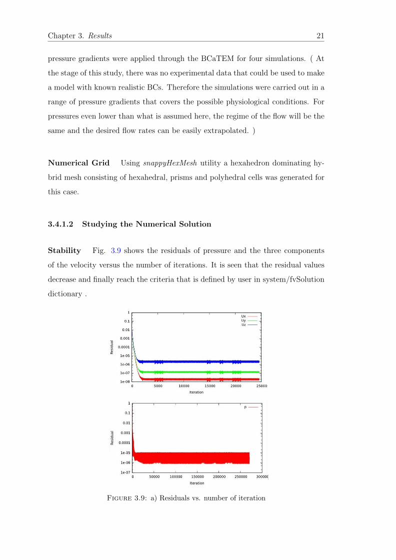
Stability Fig. 3.9 shows the residuals of pressure and the three components

of the velocity versus the number of iterations. It is seen that the residual values

decrease and finally reach the criteria that is defined by user in system/fvSolution

dictionary .

Figure 3.9: a) Residuals vs. number of iteration


Convergence The same simulations were carried out for grids with different

cell numbers and the deviation of the calculated volumetric fluxes were less than

2%. table.3.1

Level of Type and Number Volumetricrefinement of the Cells Flux[m3/s]

(1,1) hexahedra: 268304, prisms: 25944 polyhedra: 30824 4.46E-021(3,3) hexahedra: 1033864, prisms: 105988 polyhedra: 170118 4.42E-021

Table 3.1: The volumetric flux calculated at the outlet of BCaTEM in differentgrids

Studying the Flow The logarithmic values of volumetric flow rates versus

pressure gradients are depicted in Fig.3.10. The slope of the resulting line is equal

to one, showing that the flow has laminar behavior in the range of applied pressure

gradients (10−3 − 105 (Pa) ∼ 0.00010 - 10 197.16 mm water at 4◦ C).

Figure 3.10: The logarithmic values of volumetric flux (m3/s)vs pressure (Pa)gradient


Visualization of the Numerical Solution To visualize the numerical solu-

tion, the results of one of the simulations that was done with pressure gradient

of 10(Pa)are shown here. Fig.3.11 shows the pressure distribution through the

whole structure. It can be seen that the maximum value occurs at the inlet and

the minimum value at the outlet in agreement with the mentioned BCs. In order

to see the velocity profile inside the BCa, it was cut in two locations Fig. 3.12

and Fig. 3.13 using the slice utility in Paraview [17]. As it was expected, the

magnitude of velocity is zero in the proximity of the rigid walls and the maximum

velocity happens far from the walls where there is the minimum friction to flow.

Figure 3.11: Pressure gradient through BCa2D reconstructed from TEM data.The values of P(N.m/kg) are density normalized


Figure 3.12: Velocity(m/s)profile in one plane cut in BCa2D.

Figure 3.13: Velocity(m/s) profile in another plane cut in BCa2D. the bluesquare corresponds to a dead end with no flow


3.4.2 Computational Fluid Dynamics Simulations of 3D

Bile Canaliculus

The simulations were carried out for two different BCas reconstructed from SBF-

SEM 3D data, Fig.3.14. The components of the numerical solutions and the results

are explained here.

Figure 3.14: The length and the average diameter of BCa1(upper) andBCa2(lower).

3.4.2.1 Components of the Numerical Solution


for the bile flow as an incompressible and Newtonian fluid and in steady state

mode. Under these assumptions, the continuity and Navier-Stokes equations can

be simplified to eq.(3.1) and eq.(3.2).

Boundary Conditions In order to apply a pressure gradient between two ends

of the BCas, a nonzero uniform pressure was considered for the inlet (one of the


two ends) and for the outlet (the other end) the total pressure was chosen to be

zero. All the other surfaces were considered as rigid walls with no slip BCs.

Numerical Grid Using snappyHexMesh utility a hexahedron dominating hy-

brid mesh consisting of hexahedral and polyhedral cells was generated for both

cases.

3.4.2.2 Study of the Numerical Solution

Stability Fig.3.15 shows the residuals versus the number of iterations. In both

cases, the residuals for all variables decrease as the number of iterations increases.

Finally they reach blow the preset value and remain almost constant with negligible

fluctuations around it.

Figure 3.15: Residuals of pressure and velocity vs the number of iterationsfor BCa1(left) and BCa2(right).


Convergence Table.3.2 shows the results of Mesh study for this geometry in

two different mesh sizes acquired by using different levels of refinement in snappy-

HexMesh.

Structure Level of Type and Number Volumetricname Refinement of the Cells Flux [m3/s]BCa1 (4,4) hexahedra: 2399516 — polyhedra: 496370 2.58E-018BCa1 (3,3) hexahedra: 596225 — polyhedra: 109564 2.56E-018BCa1 (1,1) hexahedra: 29936 — polyhedra: 1123 2.44E-018BCa2 (4,4) hexahedra: 1242971 — polyhedra: 237236 7.81E-019BCa2 (3,3) hexahedra: 294935 — polyhedra: 50340 7.76E-019BCa2 (1,1) hexahedra: 14342 — polyhedra: 832 7.08E-019

Table 3.2: The volumetric flux calculated in different grids for BCa1 ans BCa2

Study of The Flow The logarithmic values of volumetric flow rates versus

pressure gradients are depicted in Fig.3.16. The slopes of the lines are equal to one.

It shows that the flow is in laminar regime for the applied pressure gradients(10−3−

105 (Pa) ∼ 0.00010 - 10 197.16 mm water at 4◦ C), in both cases.

Figure 3.16: The logarithmic values of volumetric flux (m3/s) vs pressure(Pa) gradient

Visualization of the Numerical Solution Fig.3.17-left shows the pressure

streamlines for the pressure gradient. The non-uniform distribution of pressure is

due to the presence of MV and the other objects inside the BCa. These objects


that are reconstructed from EM images can be easily tracked in corresponding

frames which are available in accompanying DVD. Their identities are not clearly

known yet. Here, they are modeled as stationary objects and their surfaces are all

considered as rigid walls with no slip BCs.

Fig.3.17-right shows the streamlines of the velocity. To have a closer look to the

velocity profile inside the BCas, they are cut in two regions using slice utility

in paraView and the results are shown in Fig.3.18-3.21 The minimum velocity

happens close to the rigid walls and the maximum velocity appears in a region far

from obstacles and walls.

Figure 3.17: The streamlines of pressure(The values of P(N.m/kg) are densitynormalized) and velocity(m/s) in BCa1 and BCa2


Figure 3.18: Velocity(m/s) profile in one plane perpendicular to the bile flowin BCa1.

Figure 3.19: Velocity(m/s) profile in one plane perpendicular to the bile flowin BCa1 .

Chapter 4

Discussion

4.1 Simulations of The Bile Flow in Bile Canali-

culi

The laminar flow of bile as an incompressible and Newtonian fluid was simulated as

a steady state case in BCaTEM, BCa1 and BCa2 in a range of pressure gradients.

To study the stability and the convergence of the numerical solutions, the same

simulations were carried out in grids with different cell numbers, Table.3.1and

Table.3.2. The calculated volumetric fluxes are very close (with a difference less

that 2%) which implies the convergence of the solution in all three cases. The

illustrated 2D contours of velocity and pressure are in agreement with the applied

BCs and the geometrical features of the BCas. The same is true about the 3D

streamlines of pressure and velocity for BCa1 and BCa2.

Fig.4.1 shows the logarithmic values of volumetric fluxes at the outlet of BCas

versus the applied pressure gradients for all BCas studied in chapter 3. BCa1 shows

a higher volumetric flux in comparison with BCa2. This result is in agreement

with its geometrical features in comparison with BCa2 which has a longer length

and smaller average diameter Fig.3.14. BCaTEM has a much less volumetric flux

in comparison to BCa1 and BCa2. Although its length is about half of the BCa1,

it has an average diameter of about 200nm and the minimum diameter of 6nm

31

Chapter 4. Discussion 32

Fig.3.3. It seems that the flow rate in BCaTEM was highly influenced by its

minimum diameter.

Figure 4.1: log(Q(m3/s))-log(P(Pa)) diagrams for all three reconstructedBCas

4.2 Equivalent Diameter

In Hagen–Poiseuille flow, we have the following relationship between the flow prop-

erties and the geometrical features of the pipe:

Q · µ∆P

=πD4

128L(4.1)

Multiplying both sides of eq.4.1 by L, the right side becomes a function of D. D

can be also perceived as the hydraulic diameter, which is equal to actual diameter

of pipe in Hagen–Poiseuille flow. By following the same analysis for BCa1 and

BCa2, their equivalent hydraulic diameters are calculated as: DBCa1 ∼ 482nm

and DBCa2 ∼ 411nm. Using this analysis each BCa can be treated as a smooth


pipe with a length equal to the total length of the BCa and a diameter equal to

the calculated equivalent hydraulic diameter.

4.3 Summary and Conclusion

In this project, by taking advantage of the available free source softwares and two

common commercial packages, the realistic structures of BCas were reconstructed

from SBF-SEM 3D data. At the time of writing this thesis, these images are

considered the best result of compromising between, high resolution, less damage

and high signal to noise ratio. However the proposed pipe-line for reconstruction

has the flexibility of being applied to other 3D data with higher resolution and

better quality.

The reconstructed structures were used as surface meshes to generate 3D numerical

grids using snappyHexMesh utility in openFoam. The flow of bile through these

complex geometries was modeled as steady state and laminar flow through rigid

walls with no-slip boundary conditions. Due to the lack of the experimental data,

the flow was simulated in a range of pressure gradients that could be valid under

physiological conditions.The resulting equations were solved using SIMPLEFOAM

solver in openFoam. The convergence and the stability of numerical solutions were

investigated. To get a visualization of the flow parameters, the 2D contours in

different planes and the 3D streamlines of velocity and pressure were calculated

and illustrated in chapter 3. It was also shown that, they were in agreements

with assumed BCs. Finally, by comparing the flow parameters with those of

Hagen–Poiseuille flow, the equivalent hydraulic diameters, independent of pressure

gradient magnitude were calculated for BCa1 and BCa2.

In conclusion, it was shown that, using available open source and two commonly

used commercial packages, one could get a realistic 3D reconstruction of BCas on

the basis of any 3D data such as SBF-SEM images. For the resulting complex

geometries, high quality 3D numerical grids with mostly hexagonal cells could

be generated for finite volume based simulations. The results could be used to

calculate effective hydraulic diameter which was in agreement with the geometrical


features of the reconstructed BCas.

It is also worth mentioning that in spite of the geometrical differences between

BCa1 and BCa2, the flow properties and hence the calculated equivalent diameters

were very similar which might suggest the homogeneity of flow properties in BCa

network. However, one must be aware of the fact that the flow simulations were

carried out only for fully open BCas that were clearly observable in the studied

images which belonged to one small portion of a lobule in liver(i.e. ∼ 30− 40%of

the detected BCas in one sample with the size of 75µm × 75µm × 80µm ).

Therefore, to generalize the obtained results to all the BCas in a lobule or in the

liver requires a wider statistical sampling and analysis.

4.4 Future Prospects

Experimental data at the level of these simulations are not achievable at the mo-

ment. Therefore, it is not possible to validate the proposed model and the results

of the simulations on the basis of experiments. However, one way of studying the

validity of this model and the simulations is to use the equivalent Hagen–Poiseuille

pipes in a circuit model representing the 3D web of BCas in a larger scale, that

is achievable in experiments and to compare the calculated results with the real

data.

In order to get a more realistic model of bile flow in BCas, the boundary conditions

must be selected in more agreement with experimental knowledge. For example

some modifications can be done by considering sources of inlet on MVs ( This was

done in this project, however the results were not presented in this thesis as the

assumed mass flow rate magnitudes could not be experimentally verified and it

would add to the complexity of the analysis), by taking into account the actual

direction of the flow and including the possible motility of BCas as reported by

Watanabe et al.[16] and the poro-elasticity of MV in the model. However to add

any of these modifications to the proposed simple model requires reliable exper-

imental data that can shed a light on the actual rate of the bile secretion from

the hepatocytes to the lumen of a single BCa, the position of the BCas in the


lobule, the dynamics of BCa contraction and the elasticity of MVs. None of these

information was available at the time of doing this project.

It is also suggested to run the flow simulations on more reconstructed BCas that

are selected from different regions of the lobule. Then the results can be compared

and analyzed statistically in order to get a better idea about the homogeneity of

the equivalent diameter through the whole lobule.

Appendix A

Verification of The Solver

A.1 Simulating the Flow of Liquid Water

in Simple Geometries

In order to validate the solver, two classical problems in fluid mechanics were

solved using simpleFoam and the results were compared to the theoretical solu-

tions to study its accuracy. These include the flow of liquid water between two

parallel plates and the Hagen–Poiseuille flow .

A.1.1 The Flow Between Two Parallel Plates

A.1.1.1 Components of the Numerical Solution


for the incompressible fluid and the fully developed and steady state flow in y

direction between two identical and stationary parallel plates with 500 m length,

100 m width and a 1 m gap between in z direction. Under these assumptions, the

continuity and Navier-Stokes equation in Cartesian coordinates can be simplified

to Eq.A.1 and Eq.A.2:

37

Appendix A. Verification of Solver 38

∇ · v = 0 (A.1)

∂p

∂y= µ

∂2v

∂z2(A.2)

Boundary Conditions A uniform pressure of 10−5 (Pa) was applied to the

inlet and for the outlet the total pressure was chosen to be zero. The plates were

considered as stationary rigid walls with no-slip BC:

Numerical Grid For this problem a regular H type grid was generated using

blockMesh utility in openFoam.

A.1.1.2 Study of the Numerical solution

Convergence and Accuracy Fig.A.1 shows the convergence of the volumetric

flow rate ( m3/s) value, that is calculated numerically, towards the analytical

solution. By decreasing the size of the mesh, the final solution gets closer to the

analytical answer. Finally the solution becomes independent of mesh size with an

error of 1% compared to the analytical solution.

Visualization of the Numerical Solution Fig.A.2a shows the pressure gra-

dient between the inlet and outlet. The maximum and minimum pressure mag-

nitudes are in agreement with BCs. Fig.A.2-b shows the velocity profile parallel

and perpendicular to the direction of the flow.


0 0.5 1 1.5 2 2.5x 105

1

1.5

2

2.5

3

3.5

4

4.5

x 10−4

Number of cells in Grid

outF

low

(m3/

s)

Mesh Convergence for Flow Between Two Parallel Plates

Calculated Value

Theoretical Value

Figure A.1: Convergence of the calculated flux to the analytical value

Figure A.2: a)Pressure gradient (The values of P(N.m/kg) are density nor-malized) b)velocity (m/s) profile in a plane parallel with the flow c) velocity

profile in a plane perpendicular to the flow


A.1.2 Simulating Hagen–Poiseuille Flow

A.1.2.1 Components of the Numerical Solution

Mathematical Model Hagen–Poiseuille Flow is the fully developed, steady

state and laminar flow of an incompressible and Newtonian fluid through a smooth

pipe with circular cross section. In this case the continuity and Navier-Stokes

equations in Cylindrical coordinates can be simplified to equation (A.1)and(A.3):

1

r

∂

∂r

(r∂uz∂r

)=

1

µ

∂p

∂z(A.3)

The pipe studied in this section has a length of 200 m and a diameter of 2 m.

Boundary Conditions A uniform pressure of 10−7 (Pa) was applied to the

inlet and for the outlet the total pressure was chosen to be zero. The circular wall

was considered as stationary rigid wall with no-slip BC.

Numerical Grid For this case, an irregular hexahedron dominating grid was

generated using snappyHexMesh utility, to investigate the convergence of the so-

lution in irregular grids

A.1.2.2 Study of the numerical solution

Convergence and Accuracy Fig.A.3 shows the convergence of the volumetric

flow rate (m3/s) values, that were calculated numerically,to the analytical solution

equation.A.4. By increasing the number of cells in the mesh, the final solution gets

closer to the analytical answer. Finally the solution becomes independent of mesh


size with an error of 2% compared to the analytical solution.

∆P =8µLQ

πr4(A.4)

1 1.5 2 2.5 3 3.5 4 4.5 53.1

3.15

3.2

3.25

3.3

3.35

3.4

3.45

3.5

3.55

3.6x 10−6

Level of Refinement

outF

low

(m3/

s)

Hybrid Mesh Convergence for Poiseuille Flow

Calculated value

Theoretical Value

Figure A.3: Convergence of the calculated volumetric flux (m3/s) to theanalytical value

Visualization of the numerical Solution Fig.A.4shows the numerically cal-

culated pressure gradient between the inlet and outlet. Fig.A.5 shows the ve-

locity profile parallel and perpendicular to the direction of flow. One can see the

parabolic shape of the velocity profile predicted by equation.A.5 and also the mag-

nitude of maximum velocity that occurs at the center of the tube.

v = − 1

4η

∆P

∆z(R2 − r2) (A.5)


Figure A.4: Pressure gradient (The values of P(N.m/kg) are density normal-ized) through the pipe

Figure A.5: (left)velocity profile (m/s) in a plane perpendicular to theflow(right)velocity (m/s) profile in a plane parallel with the flow

Appendix B

Serial Block-Face Scanning

Electron Microscopy Setup

Different setups of SBF-SEM that were investigated to obtain the best compromi-

sation between the minimum beam damage to the samples, the higher resolution

in z direction and the higher signal to noise ratio are listed in Table B.1.

The pixel size in X-Y plane had been already optimized by EM facility in MPI-

CBG.

settings acceleration electron beam dwell pixel size X [nm] × Y [nm]label voltage [kV] intensity [pA] time [µs] Z-resolution[nm]S1 1.5 100 0.8 12.4× 12.4|40S2 1.5 + 0.1 Bias 200 0.6 12.5× 12.5|30S3 1.5 100 1.2 12.5× 12.5|25

Table B.1: Different SBF-SEM setups.

S1 revealed the images with the least introduced damage as the sections were

thicker and the damaged area was completely removed by cutting. However the

resolution in z direction was the lowest in S1, since the cut slices in S1 were thicker

in comparison with slices in S2 and S3. In S2, the higher resolution was obtained

in the expense of more cutting artifacts to the sample Fig.B.1.This was mainly

because of the more beam damage that resulted in improper cutting and the fall

of some of the cut areas of the previous section . The resulting images in S3 had

43

Appendix B. Serial Block-Face Scanning Electron Microscopy Setup 44

higher resolution, no serious beam damage to the sample and no cutting artifacts,

but a very low signal to noise ratio Fig.B.2. This problem can be related to the

charging of the sample or the variability in sample staining. Unfortunately, the

number of the detected open BCa were not enough for reconstruction and flow

studies. Therefore it was not possible to judge the benefits of using S3 over S1. In

conclusion S1, with the least introduced beam damage to the sample, a resolution

high enough to detect the MVs and a correctable signal no noise ratio was chosen

for reconstruction.


Figure B.1: The image resulting from s2

Figure B.2: The image resulting from s3

Bibliography

[1] Malinen MM, Palokangas H, Yliperttula M, Urtti A. Peptide nanofiber hydrogel

induces formation of bile canaliculi structures in three-dimensional hepatic cell

culture.Tissue Eng Part A. 2012 Dec.18(23-24).2418-25.

[2] Boyer JL. Bile formation and secretion. Compr Physiol. 2013 Jul.3(3).1035-78.

[3] Matsui H, Takeuchi S, Osada T, Fujii T, Sakai Y. Enhanced bile canaliculi

formation enabling direct recovery of biliary metabolites of hepatocytes in 3D

collagen gel microcavities. Lab Chip. 2012 Apr 24.12(10).1857-64.

[4] Arias IM, Che M, Gatmaitan Z, Leveille C, Nishida T, St Pierre M. The biology

of the bile canaliculus, 1993. Hepatology. 1993 Feb.17(2):318-29.

[5] Alejandro Esteller. Physiology of bile secretion. World J Gastroenterol. 2008

October 7.14(37).5641–5649.

[6] I Arias. A Wolkoff. J Boyer. D Shafritz.N Fausto. H Alter.D Cohen. The Liver:

Biology and Pathobiology. Wiley-BlackWell. 5th Edition. 2009

[7] Denk W, Horstmann H. Serial Block-Face Scanning Electron Microscopy to

Reconstruct Three-Dimensional Tissue Nanostructure. PLoS Biol.(2004).2(11).

[8] Xiaoyu Luo, Wenguang Li, Nigel Bird, Swee Boon Chin, NA Hill, Alan G

Johnson. On the mechanical behavior of the human biliary system. World J

Gastroenterol.2007 March 7.13(9).1384-1392

[9] Al-Atabi M, Ooi RC, Luo XY, Chin SB, Bird NC. Computational analysis of

the flow of bile in human cystic duct. Med Eng Phys. 2012 Oct. 34(8).1177-83

47


[10] Soto GE, Young SJ, Martone ME, Deerinck TJ, Lamont S, et al. Serial section

electron tomography: A method for three-dimensional reconstruction of large

structures. Neuroimage. 1994.1:230–243.

[11] T Blacker. Automated Conformal Hexahedral Meshing Constraints, Chal-

lenges and Opportunities.Engineering with Computers.(2001).17.201–210

[12] Ooi RC, Luo XY, Chin SB, Johnson AG, Bird NC. The flow of bile in the

human cystic duct J Biomech. 2004 Dec.37(12).1913-22.

[13] Yamamoto K, Itoshima T, Tsuji T, Murakami T. Three-dimensional fine

structure of the biliary tract: scanning electron microscopy of biliary casts. J

Electron Microsc Tech. 1990 Mar.14(3).208-17.

[14] Alejandro Esteller. Physiology of bile secretion. World J Gastroenterol. 2008

October 7.14(37).5641–5649.

[15] openFoam online User’s Guide at http://www.openfoam.org/docs/user/

[16] Watanabe N, Tsukada N, Smith CR, Phillips MJ. Motility of bile canaliculi in

the living animal: implications for bile flow.J Cell Biol. 1991 Jun.113(5):1069-80.

[17] paraView user’s guide at http://www.paraview.org/paraview/help/download/

[18] J H Ferziger, M Peric.Computational Methods for Fluid Dynamics. Springer.

3rd Edition. 2001

numerical simulations of bile flow in realistic image

Documents