REPORT DOCUMENTATION PAGE "" " No 07040186

", •..... ........ o. . . ....'.n u - - .. ,.. . .... , .. . ... . ........ .- 4 a- .... :,- . w. ., + , -... .~ .. ....*... 2 J ..... Ib . . ...n.sc t... -. . 3. . .. ;,,-

1. AGENCY USE ONY (Leike biani) j2. REPORT DAT& 13.. RPORT TYPE AND DATES COVERED

4 NOV 93 I THESIS/DISSERTATION4. TITLE AND SUBTITLE S. FUNDING NUMBERS

• [! NUMERICAL SIMULATIONS OF A MOUNTAIN THUNDERSTORM: A

•%• COMPARISON WITH DOPPLER RADAR OBSERVATIONS

1• 6. AUTHOR•(S)

P a MARK EDWIN RAFFENSBERGER

7. PERFORMING C.-GANIZATION NAME(S) AND ADDRESS(ES) S. PERFORMING ORGANIZATION

AFIT Student Attending: THE FLORIDA STATE UNIVERSITY AFIT/CI/CIA- 93-155

9. SPONSORING/MONITORING AGENCI NAME(S) AND ADDRESS(ES) 10. SPONSORING/MONITORING

DEPARTMENI OF THE AIR FORCE AGENCY REPORT NUMBER

AFIT/CI2950 P STREETWRIGHT-PATTERSON AFB OH 45433-7765

11. SUPPLEMENTARY NOTES

12a. DISTRIBUTION /AVAILABILITY STATEMENT 12b. DISTRIBUTION CODE

Approved for Public Release IAW 190-1Distribution Unlimited -R

MICHAEL M. BRICKER, SMSgt, USAFChief Administration __

13. ABSTRACT (Maximun 200 words) T F_

04: 1994

S94-03971ýl flldlllIV111

S2 03 185I14. SUBJECT TERMS 15. NUMBER OF PAGES

21216. PRICE CODE

17. SECURITY CLASSIFICATION 18. SECURITY CLASSIFICATION 19. SECURITY CLASSIFICATION 20. LIMITATION OF ABSTRACT

OF REPORT OF THIS PAGE OF ABSTRACT

NSN 7540-01-280-5500 Stanoard Form 298 (Rev 2-89)

A .k

DEPARTMENT OF THE AIR FORCEUSAF ENVIRONMENTAL TECHNICAL APPUCATIONS CENTER (AWS)

SCOTT AIR FORCE BASE, ILLINOIS

From: USAFETAC/SYT (Capt Raffensberger, DSN 576-5412) 4 Nov 93859 Buchanan St, Rmn 403Scott AFB IL 62225-5116

Subj: AFIT Program Completion (Our Telecon, 3 Nov 93)

To: AFIT/CIR (Maj Smith)

1. The purpose of this letter is to notify you that I have completed my AFIT-sponsoredMaster's Degree program at Florida State University. I have enclosed at Atch 1 a copy of mythesis entitled "Numerical Simulations of a Mountain Thunderstorm: A Comparison WithDoppler Radar Observations." I have also enclosed at Atch 2 two copies of the abstract forthe thesis.

2. I will arrange for Florida State University to forward an official transcript to you when thedegree is posted (mid- to late-December).

3. Thank you for your assistance. If you require any additional information, please contactme at DSN 576-5412.

MARK E. RAFFENSBERGER, Capt, USAF 2 Atch1. Thesis2. Thesis Abstract (2 copies)

Accesion ForNTIS CRA&IDTIC TAB 0Unan(Iou::cedJtistificatiobn

y.....................B y .................................................Dist ibJtiolf

A�',i:O~iMV rCdes DTO QUALITY IN8ECTEDI Ast a,

Dist Sgrc~iai

THE FLORIDA STATE UNIVERSITY

COLLEGE OF ARTS AND SCIENCES

NUMERICAL SIMULATIONS OF A MOUNTAIN THUNDERSTORM:

A COMPARISON WITH DOPPLER RADAR OBSERVATIONS

BY

MARK EDWIN RAFFENSBERGER

A Thesis submitted to theDepartment of Meteorologyin partial fulfillment of the

requirements for the degree ofMaster of Science

Degree Awarded:

Fall Semester, 1993

The members of the Committee approve the thesis of Mark E. Raffensberger de-

fended on October 28, 1993.

Professor Directing Thes

6mrittee Member

Noel E. LaSeurCommittee Member

Kenneth W. JohM nCommittee Member

ACKNOWLEDGEMENTS

Many people have contributed their time, talent, and resources to help me com-

plete this research. I extend my deep appreciation to Dr. Peter S. Ray, my advisor,

for his many useful suggestions, valuable guidance, and tremendous encouragement

and patience. I am most grateful to my committee members, Dr. Ken Johnson, Dr.

J.J. Stephens, and Dr. Noel LaSeur for their careful reviews of this manuscript and

for their many thoughtful comments and suggestions. I especially thank Dr. Ken

Johnson for his unending patience and advice in helping me adapt to many new com-

puter systems along the way. I also thank Dr. William Cotton, Dr. Greg Tripoli,

Craig Tremback, and other members of Dr. Cotton's group for the advice and sug-

gestions they provided on using their model. I offer many thanks to Mary Stephen-

son, Dr. B.J. Sohn, Dr. Mohan Ramamurthy, Steve Lang, Terry Given, Russ

Treadon, and especially Dr. Ying Lin and Anna Nelson Smith, and the many others

who helped me at FSU. I thank the United States Air Force for supporting my educa-

tion through the Air Force Institute of Technology Civilian Institutions program and

all my supervisors and coworkers at Air Weather Service who encouraged me to fin-

ish this work. To my parents, James and Loretta, I offer my deep thanks for instill-

ing in me the desire to continue my education. To my daughters, Emily and

Gretchen, I offer my appreciation for their patience while I spent countless nights and

weekends in front of the computer and away from them. Finally, I offer my deepest

gratitude to Donelle, my wife, for her all her loving support, sacrifice, encourage-

ment, and good counsel without which I could not have succeeded.

iii

TABLE OF CONTENTS

List of Tables .................................................. vii

List of Figures ................................................. viii

List of Abbreviations and Symbols ................................ xviii

Abstract ....................................................... xx

Chapter 1. Introduction .......................................... I

Chapter 2. Historical Review of Mountain Thunderstorms ............... 4

2.1 Observational studies ........................................ 4

2.2 Numerical modeling studies .................................. 11

Chapter 3. Observations of the 31 July 1984 Storm and Its Environment ... 15

3.1 New Mexico Mountain Thunderstorms ............................. 15

3.2 Data collection and analysis .................................. 16

3.2.1 Facilities ............................................. 16

3.2.2 Rawinsonde observations ................................. 18

3.2.3 Doppler radar observations and analyses ..................... 21

3.2.4 Doppler-derived environmental wind profiles .................. 24

3.2.5 Local terrain .......................................... 25

3.3 31 July 1984 storm history: Radar observations ................... 25

3.3.1 Pre-storm development .................................. 29

3.3.2 Storm initiation and early development ...................... 29

3.3.3 Mature storm development ............................... 31

iv

3.3.4 Storm decay .......................................... 54

3.3.5 Summary ............................................. 61

Chapter 4. The Numerical Model .................................. 65

4.1 M odel selection ........................................... 65

4.2 Model ability to simulate mountain storms ....................... 66

4.3 Model description .......................................... 67

4.4 Horizontal grid structure .................................... 70

4.5 Vertical grid structure ...................................... 71

4.6 Model topography ......................................... 74

4.7 Initialization .............................................. 74

Chapter 5. Experimental Design ................................... 78

5.1 Control simulation configuration ............................... 78

5.2 Atmospheric base-state profiles ................................ 79

5.2.1 Temperature and moisture profiles .......................... 80

5.2.2 W ind profiles ......................................... 81

5.2.2.1 Preliminary composite profile ......................... 83

5.2.2.2 Base-state wind profiles .............................. 83

5.3 Numerical experiments ...................................... 86

Chapter 6. Analysis and Verification of the Control Simulation .......... 92

6.1 Analysis of simulated storm evolution ........................... 95

6.2 Comparison with radar observations ........................... 121

6.2.1 General comparisons ..................................... 124

6.2.2 Detailed comparisons ................................... 132

6.3 Comparison with microphysical retrievals ....................... 141

V

Chapter 7. Sensitivity to Wind Flow ............................... 146

7.1 Experiment 1 - No Wind Case: Analysis of simulated storm evolution . 146

7.2 Experiment 1 - No Wind Case: Comparison with Control .......... 154

7.3 Experiment 2 - 50% Wind Case ................................. 160

Chapter 8. Sensitivity to Diabatic Heating Effects .................... 162

8.1 Experiment 3 - No Short Wave Radiation Case ................... 162

8. 1.1 Analysis of simulated cloud evolution ...................... 162

8.1.2 Comparison with Control ................................ 164

8.2 Experiment 4 - Warm Rain Microphysics Case ................... 164

8.2.1 Analysis of simulated storm evolution ...................... 164

8.2.2 Comparison with Control ................................ 172

Chapter 9. Sensitivity To Initial Moisture Profile ..................... 179

9.1 Experiment 5 - Moistened Lower Levels Case ................... 179

9.2 Analysis of simulated storm evolution .......................... 179

9.3 Comparison with Control ................................... 195

Chapter 10. Conslusions ........................................ 200

References .................................................... 208

Biographical Sketch ............................................ 213

vi

LIST OF TABLES

Table 1: Model vertical grid structure for vertical velocity grid points ......... 73

Table 2: Soil model base-state soil moisture profile. Soil moisture given aspercentage of saturated soil moisture . ................................. 79

Table 3: Numerical simulation experiment overview. "Standard" refers to condition

or process employed in the control simulation ......................... 90

Table 4: Simulation time to actual time conversion chart .................. 93

Table 5: Model height to actual height conversion ........................ 94

vii

LIST OF FIGURES

Fig. 1. Radar network and topographical view of terrain features near LangmuirLaboratory. Terrain elevation is relative to mean sea level in kilometers and contourintervals are every 0.2 km. The horizontal and vertical axes are labeled in kilome-ters. The origin (0,0) is located at Langmnuir Laboratory. A sample radar analysisdomain is shown for reference . ...................................... 17

Fig. 2. Skew T, log P plot of the 0719 MST 31 July 1984 Socorro Airportthermodynamic sounding. Solid skewed lines are temperatures in degrees Celsius;dashed skewed lines are mixing ratios in grams per kilogram; curved dashed lines aredry adiabats in degrees Celsius; solid horizontal lines are pressures in millibars.Heavy solid and dashed lines represent sensible and dewpoint temperature profiles,respectively . .................................................... 19

Fig. 3. As in Fig. 2, 0945 MST 31 July 1984 Langmuir Laboratory thermodynamicsounding . ...................................................... 20

Fig. 4. Vertical profiles of estimated u (solid curve) and v (dashed curve) wind com-ponents from Ziegler, personal communication (1986). The horizontal axis is windspeed in meters per second, and pressure in millibars is along the vertical axis. .. 22

Fig. 5. Vertical profile of Doppler-derived u (solid curve) and v (dashed curve) windcomponents calculated as described in text using Doppler-derived wind data from theperiod between 0946 and 1019 MST. Axes labeled as in Fig. 4 ............. 26

Fig. 6. Vertical profile of Doppler-derived u (solid curve) and v (dashed curve) windcomponents calculated as described in text using Doppler-derived wind data from theperiod between 1116 and 1216 MST. Axes labeled as in Fig. 4 ............. 27

Fig. 7. Topographical view of terrain features near Langmuir Laboratory. Terrainelevation is relative to sea level in dekameters and contour intervals are every 20dekameters. The horizontal and vertical axes are labeled in kilometers. The origin(0,0) is located at Langmuir Laboratory. Valleys and ridges are labeled as describedin text . ........................................................ 28

Fig. 8. Horizontal cross-section of observed radar reflectivities in dBZ and vectorvelocities at an altitude of 3.3 km relative to mean sea level at 1119 MST 31 July1984. Reflectivities (solid contours) are contoured every 10 dBZ. Vector velocitiesare iround-relative with a vector length of one grid interval (0.5 kin) equal to 15m s . Terrain elevations (dashed contours) are relative to sea level in meters, andcontour intervals are every 200 meters. The origin is at Langmuir Laboratory, andthe axes are labeled in kilometers . .................................... 30

viii

Fig. 9a. Horizontal cross-section of observed radar reflectivities and vector velocitiesas in Fig. 8, except at 1134 MST and at 3.3 km MSL .................... 32

Fig. 9b. As in Fig. 8, horizontal cross-section of observed radar reflectivities andvector velocities for 1134 MST and at 7.3 km MSL ..................... 33

Fig. 10a. Horizontal cross-section of observed radar reflectivities in dBZ at an alti-tude of 4.3 km relative to mean sea level at 1140 MST 31 July 1984. Reflectivitiesare contoured every 5 dBZ. The origin is at Langmuir Laboratory. The axes are la-beled in kilometers. Line AB shows the location of the vertical cross-section in Fig.10b . .......................................................... 35

Fig. 10b. Vertical cross-section of observed radar reflectivities in dBZ and vectorvelocities at 1140 MST 31 July 1984. Reflectivities are contoured every 5 dBZ.Vector velocities are ground-relative with the vector length shown in upper right-handcomer of figure equal to 20 m s'. Cross-section location AB is shown in Fig. 10a.

............................................................. 36

Fig. I1 a. Horizontal cross-section of observed radar reflectivities and vector veloci-ties as in Fig. 8, except at 1146 MST and at 3.3 km MSL ................. 38

Fig. I1 b. As in Fig. 8, horizontal cross-section of observed radar reflectivities andvector velocities for 1146 MST and at 9.3 km MSL ..................... 39

Fig. 12a. Horizontal cross-section of observed vertical velocities at an altitude of 3.3km relative to mean sea level at 1146 MST 31 July 1984. Velocities are contouredevery 3.0 m s' starting at 0 m s-1. Solid contours denote upward vertical velocities(positive w), and dashed contours denote downward vertical velocities (negative iv).Origin and axes are as in Fig. 8 . ..................................... 40

Fig. 12b. Horizontal cross-section of observed vertical velocities at 1146 MST 31July 1984 as in Fig. 12a, except at 8.3 km MSL ....................... 41

Fig. 13. As in Fig. 8, horizontal cross-section of observed radar reflectivities andvector velocities for 1149 MST and at 7.3 km MSL ..................... 43

Fig. 14a. Horizontal cross-section of observed vertical velocities as in Fig. 12a, ex-cept at 1149 MST and at 3.3 km MSL. Labels indicate locations of updrafts asso-ciated with cells C1 and C2 . ........................................ 44

Fig. 14b. As in Fig. 12a, horizontal cross-section of observed vertical velocities for1149 MST and at 6.3 km MSL. Labels indicate locations of updrafts associated withcells C l and C2 . ................................................. 45

Fig. 15a. Horizontal cross-section of observed radar reflectivities as in Fig. 10a, ex-cept at 1152 MST and 4.3 km MSL. Lines AB and CD show locations of verticalcross-sections in Figs. 15b and 15c, respectively ....................... 47

Fig. 15b. As in Fig. 10b, vertical cross-section of observed radar reflectivities andvector velocities at 1152 MST. Cross-section location AB is shown in Fig. 15a. . 48

ix

Fig. 15c. As in Fig. 10b, vertical cross-section of observed radar reflectivities andvector velocities at 1152 MST. Cross-section location CD is shown in Fig. 15a. . 49

Fig. 16. Horizontal cross-section of observed radar reflectivities and vector velocitiesas in Fig. 8, except at 1158 MST and at 8.3 km MSL ..................... 50

Fig. 17a. As in Fig. 10a, horizontal cross-section of observed radar reflectivities at1158 MST and 4.3 km MSL. Lines AB and CD show locations of vertical cross-sections in Figs. 17b and 17c, respectively ............................. 51

Fig. 17b. Vertical cross-section of observed radar reflectivities and vector velocitiesas in Fig. 10b, except at 1158 MST. Cross-section location AB is shown in Fig. 17a.

..................................................... 52

Fig. 17c. Vertical cross-section of observed radar reflectivities and vector velocitiesas in Fig. 10b, except at 1158 MST. Cross-section location CD is shown in Fig. 17a.

................................................ 53

Fig. 18. As in Fig. 8, horizontal cross-section of observed radar reflectivities andvector velocities for 1204 MST and at 6.3 km MSL ....................... 55

Fig. 19a. As in Fig. 10a, horizontal cross-section of observed radar reflectivities at1204 MST and 4.3 km MSL. Line CD shows location of vertical cross-section inFig. 19b. Line AB was not used .................................... 57

Fig. 19b. Vertical cross-section of observed radar reflectivities and vector velocitiesas in Fig. 10b, except at 1204 MST. Cross-section location CD is shown in Fig. 19a.... . .............................................. 58

Fig. 20. Horizontal cross-section of observed radar reflectivities and vector veloci-ties as in Fig. 8, except at 1213 MST and at 7.3 km MSL .................. 60

Fig. 21. "Three-dimensional" model terrain elevation data. Terrain elevations arerelative to lowest terrain value in grid domain after smoothing as described in text.Terrain elevations are labeled in dekameters and contoured every 20 dekameters. Thehorizontal and vertical axes are labeled in kilometers. The origin (0,0) is located atLangmuir Laboratory ............................................. 75

Fig. 22. "Two-dimensional" model terrain elevation data. Terrain elevations arerelative to lowest terrain elevation value in slab at y = 0.0 km as described in text.Both axes are labeled in kilometers, with the origin at Langmuir Laboratory ..... 76

Fig. 23. Skew T, log P plot of base-state thermodynamic profile used to initialize thenumerical model. Heavy solid and dashed lines represent sensible and dewpoint tem-perature profiles, respectively. Skew T, log P diagram labeled as in Fig. 2..... 82

Fig. 24a. Composite vertical profile of it wind component used to construct profile toinitialize the numerical model. Heavy solid line represents preliminary compositeprofile of u wind component. Observed and estimated profiles (shown in Figs. 4, 5,and 6) are shown for reference. Axes labeled as in Fig. 4 .................. 84

x

Fig. 24b. Composite vertical profile of v wind component used to construct profile toinitialize the numerical model. Heavy solid line represents preliminary compositeprofile of v wind component. Observed and estimated profiles (shown in Figs. 4, 5,and 6) are shown for reference. Axes labeled as in Fig. 4 ................. 85

Fig. 25a. Vertical profile of the u wind component of the "three-dimensional" base-state profile (heavy solid line with ticks) used to build final profile for input to themodel. The preliminary composite profile shown in Fig. 24a is shown for reference.Axes as labeled in Fig. 4 . .......................................... 87

Fig. 25b. Vertical profile of the v wind component of the "three-dimensional" base-state profile (heavy solid line with ticks) used to build final profile for input to themodel. The preliminary composite profile shown in Fig. 24b is shown for reference.Axes as labeled in Fig. 4 . .......................................... 88

Fig. 26. Vertical wind profile used to initialize the numerical model. Wind speed inthis profile equals the magnitude of the total wind in the profiles shown in Fig. 25.Axes labeled as in Fig 4 . ........................................... 89

Fig. 27. East-west vertical cross-section of simulated total condensate mixing ratiosoverlaid with simulated wind vectors for CONTROL simulation at 6480 s. Contoursare every 2.0 g kg-' starting at 0.1 . kg-. Wind vector length shown in lower right-hand comer of figure equals 50 m s. Vertical axis is labeled in kilometers above theminimum terrain elevation in the simulation grid (in this case 1.82 kin) as describedin the text. Horizontal axis is horizontal distance labeled in kilometers. The cross-section shown is located at y = 0.0 kin and runs east-west, with the origin at Lang-muir Laboratory . ................................................ 96

Fig. 28. East-west vertical cross-section of simulated vertical velocity contoured ev-ery 3.0 m s-' starting at 1.5 m s-1 for CONTROL simulation at 6480 s. Solid(dashed) contours show positive (negative) vertical velocities. Axes labeled as in Fig.27 . .......................................................... 97

Fig. 29. East-west vertical cross-section of simulated u wind component contouredevery 3.0 m. s I starting at 1.5 in s-' for CONTROL simulation at 6480 s. Solid(dashed) contours show westerly (easterly) winds. Axes are labeled as in Fig. 27............................................................... 98

Fig. 30. East-west vertical cross-section of simulated u wind component as in Fig. 29except for CONTROL simulation at 7200 s ............................ 100

Fig. 31. Analogous to Fig. 27, east-west vertical cross-section of simulated total con-densate mixing ratios overlaid with simulated wind vectors for CONTROL simulationat 6840 s. Contour label "1" represents 0.1 g kg" ...................... 101

Fig. 32. Analogous to Fig. 28, east-west vertical cross-section of simulated verticalvelocity for CONTROL simulation at 6840 s ........................... 102

xi

Fig. 33. As in Fig. 27, east-west vertical cross-section of simulated total condensatemixing ratios overlaid with simulated wind vectors for CONTROL simulation at 7560s. Contour label "1" represents 0.1 g kg-I . ............................ 104

Fig 34. As in Fig. 28, east-west vertical cross-section of simulated vertical velocityfor CONTROL simulation at 7560 s .................................. 105

Fig. 35. East-west vertical cross-section of simulated total condensate mixing ratiosoverlaid with simulated wind vectors, as in Fig. 27, except for CONTROL simulationat 7920 s. Contour label "1" represents 0.1 g kg. ...................... 107

Fig. 36. East-west vertical cross-section of simulated vertical velocity, as in Fig. 28,except for CONTROL simulation at 7920 s ............................ 108

Fig. 37. Analogous to Fig. 27, east-west vertical cross-section of simulated total con-densate mixing ratios overlaid with simulated wind vectors for CONTROL simulationat 8100 s. Contour label "1" represents 0.1 g kg' ....................... 109

Fig. 38. Analogous to Fig. 28, east-west vertical cross-section of simulated verticalvelocity for CONTROL simulation at 8100 s .......................... 110

Fig. 39a. East-west vertical cross-section of simulated total condensate mixing ratiosoverlaid with simulated wind vectors, as in Fig. 27, except for CONTROL simulationat 8640 s. Contour label "1" represents 0.1 g kg. ...................... 113

Fig. 39b. East-west vertical cross-section of simulated cloud water mixing ratios con-toured every 2.0 g kg-1 starting at 0.1 g kg4 for CONTROL ,imulation at 8640 s.Axes labeled as in Fig. 27. Contour label "1" represents 0.1 g kg- ........... 114

Fig. 39c. Analogous to Fig. 39b, east-west vertical cross-section of simulated rainwater mixing ratios for CONTROL simulation at 8640 s. Contour label "1" repre-sents 0.1 g kg . .. . ............................................. 115

Fig. 39d. Analogous to Fig. 39b, east-west vertical cross-section of simulated pris-tine ice crystal mixing ratios for CONTROL simulation at 8640 s. Contour label "I"represents 0.1 g kg . ............................................ 116

Fig. 39e. Analogous to Fig. 39b, east-west vertical cross-section of simulated graupelmixing ratios for CONTROL simulation at 8640 s. Contour label "1" represents 0.1g kg- ... .. ................................................... 117

Fig. 39f. Analogous to Fig. 39b, east-west vertical cross-section of simulated aggre-gated snow flake mixing ratios for CONTROL simulation at 8640 s. Contour label"1" represents 0.1 g kg". ......................................... 118

Fig. 40. East-west vertical cross-section of simulated vertical velocity as in Fig. 28,except for CONTROL simulation at 8640 s ............................ 120

xii

Fig. 41. East-west vertical cross-section of simulated total condensate mixing ratiosoverlaid with simulated wind vectors, as in Fig. 27, except for CONTROL simulationat 8820 s. Contour label "1" represents 0.1 g kg. ..................... 122

Fig. 42. East-west vertical cross-section of simulated vertical velocity, as in Fig. 27,except for CONTROL simulation at 8820 s ............................ 123

Fig. 43. Time evolution of synthesized (heavy curves with ticks) and CONTROLsimulation simulated (light curves without ticks) maximum and minimum vertical ve-locities. Solid curves show maximum upward vertical velocities (positive w). Dashedcurves show maximum downward vertical velocities (negative w). Vertical axis isvertical velocity in m s1, bottom horizontal axis is simulation time in seconds, andtop horizontal axis is observation time in hours and minutes (MST) .......... 126

Fig. 44. Time-height cross section showing maximum simulated total condensateheight for the CONTROL simulation (plain curve) and maximum height of observedreflectivity (solid curve with ticks). Plain curve shows maximum height of 0.1 g kgltotal condensate mixing ratios. Ticked curve shows maximum height of 10 dBZ radarreflectivities. Right vertical axis is labeled in kilometers above the minimum terrainelevation in the simulation grid (in this case 1.82 km) as described in the text, and leftvertical axis is height relative to mean sea level in km. Bottom horizontal axis issimulation time in seconds and top horizontal axis is observation time in hours andminutes M ST . .................................................. 130

Fig. 45. Analogo,.o to Fig. 27, east-west vertical cross-section of simulated total con-densate mixing ratios overlaid with simulated wind vectors for CONTROL simulationat 8460 s. Contour label "P" represents 0. 1 g kg"4 . . . . . . . . . . . . . . . . . . . . . . 134

Fig. 46a. Horizontal cross-section of observed radar reflectivities as in Fig. 10a, ex-cept at 1134 MST and 4.3 km MSL. Line AB shows location of vertical cross-sectionin Fig. 46b. Line CD was not used . ................................. 135

Fig. 46b. As in Fig. 10b, vertical cross-section of observed radar reflectivities andvector velocities at 1134 MST. Cross-section location AB is shown in Fig. 46a.

............................................................. 136

Fig. 47. East-west vertical cross-section of simulated total condensate mixing ratiosoverlaid with simulated wind vectors, as in Fig. 27, except for CONTROL simulationat 9000 s. Contour label "1" represents 0.1 g kg' . ...................... 138

Fig. 48a. Analogous to Fig. 10a, horizontal cross-section of observed radar reflecti-vities except at 1152 MST and 4.3 km MSL. Line AB shows location of verticalcross-section in Fig. 48b. Line CD was not used ........................ 139

Fig. 48b. Analogous to Fig. 10b, vertical cross-section of observed radar reflectivi-ties and vector velocities at 1152 MST. Cross-section location AB is shown in Fig.48a . ......................................................... 140

xiii

Fig. 49. Time evolution of maximum simulated condensate mixing ratios for theCONTROL simulation. Solid curve shows total condensate mixing ratios, dot-dashcurve shows cloud water mixing ratios, dashed curve shows rain water mixing ratios,double dot-dash curve shows pristine ice crystal mixing ratios, shaded curve showsgraupel mixing ratios, and dotted curve shows aggregated snow flake mixing ratios.Vertical axis is mixing ratio in grams per kilogram. Horizontal axis is simulationtime in seconds (bottom) and in hours and seconds MST (top) .............. 143

Fig. 50. East-west vertical cross-section of simulated total condensate mixing ratiosoverlaid with simulated wind vectors for EXPI simulation at 6300 s. Contours areevery 2.0 g kg- starting at 0.1 g kg'1. Wind vector length shown in lower right-handcorner of figure equals 50 m s-. Vertical axis is labeled in kilometers above theminimum terrain elevation in the simulation grid (in this case 1.82 kin) as describedin the text. Horizontal axis is horizontal distance labeled in kilometers. The cross-section shown is located at y = 0.0 km and runs east-west, with the origin at Lang-muir Laboratory . ............................................... 147

Fig. 51. East-west vertical cross-section of simulated vertical velocity contoured ev-ery 3.0 m s-' starting at 1.5 m s-' for EXPI simulation at 6300 s. Solid (dashed) con-tours show positive (negative) vertical velocities. Axes labeled as in Fig. 50....... ............ ............ .......... .. .............. ..... 148

Fig. 52. Analogous to Fig. 50, east-west vertical cross-section of simulated total con-densate mixing ratios overlaid with simulated wind vectors for EXPI simulation at7380 s. Contour label "1" represents 0.1 g kg-' ......................... 150

Fig. 53. East-west vertical cross-section of simulated total condensate mixing ratiosoverlaid with simulated wind vectors, as in Fig. 50, except for EXPl simulation at8100 s. Contour label "1" represents 0.1 g kg- ........................ 152

Fig. 54. Analogous to Fig. 51, east-west vertical cross-section of simulated verticalvelocity for EXPl simulation at 8100 s . .............................. 153

Fig. 55. As in Fig. 50, east-west vertical cross-section of simulated total condensatemixing ratios overlaid with simulated wind vectors for EXP1 simulation at 8820 s.Contour label "1" represents 0.1 g kg-1 . .............................. 155

Fig. 56. As in Fig. 51, east-west vertical cross-section of simulated vertical velocityfor EXP1 simulation at 8820 s . ..................................... 156

Fig. 57. Time evolution of maximum simulated condensate mixing ratios for theEXPI simulation. Solid curve shows total condensate mixing ratios, dot-dash curveshows cloud water mixing ratios, dashed curve shows rain water mixing ratios, doubledot-dash curve shows pristine ice crystal mixing ratios, shaded curve shows graupelmixing ratios, and dotted curve shows aggregated snow flake mixing ratios. Verticalaxis is mixing ratio in grams per kilogram. Horizontal axis is simulation time in sec-onds (bottom) and in hours and seconds MST (top) ..................... 157

xiv

Fig. 58. Time evolution of maximum and minimum simulated vertical velocities forthe EXPI simulation. Solid curve shows maximum upward vertical velocities(positive w). Dashed curve shows maximum downward vertical velocities (negativew). Vertical axis is vertical velocity in m s-1. Horizontal axis is simulation time inseconds (bottom) and in hours and seconds MST (top) ................... 158

Fig. 59. East-west vertical cross-section of simulated total condensate mixing ratiosoverlaid with simulated wind vectors for EXP3 simulation at 8460 s. Contours areevery 2.0 g kg-1 starting at 0.1 g kgl. Wind vector length shown in lower right-handcomer of figure equals 50 m s-. Vertical axis is labeled in kilometers above theminimum terrain elevation in the simulation grid (in this case 1.82 km) as describedin the text. Horizontal axis is horizontal distance labeled in kilometers. The cross-section shown is located at y = 0.0 km and runs east-west, with the origin at Lang-muir Laboratory . ............................................... 163

Fig. 60. East-west vertical cross-section of simulated u wind component contouredevery 3.0 m s"1 starting at 1.5 m s-' for EXP3 simulation at 7740 s. Solid (dashed)contours show westerly (easterly) winds. Axes are labeled as in Fig. 59 ....... 165

Fig. 61. Analogous to Fig. 59, east-west vertical cross-section of simulated total con-densate mixing ratios overlaid with simulated wind vectors for EXP4 simulation at7920 s . ....................................................... 167

Fig. 62. East-west vertical cross-section of simulated vertical velocity contoured ev-ery 3.0 m s-1 starting at 1.5 m s" for EXP4 simulation at 7920 s. Solid (dashed) con-tours show positive (negative) vertical velocities. Axes labeled as in Fig. 59.

............................................................. 168

Fig. 63. Analogous to Fig. 59, east-west vertical cross-section of simulated total con-densate mixing ratios overlaid with simulated wind vectors for EXP4 simulation at8460 s. Contour label "1" represents 0.1 g kg- ........................ 170

Fig. 64. Analogous to Fig. 62, east-west vertical cross-section of simulated verticalvelocity for EXP4 simulation at 8460 s ............................... 171

Fig. 65. Analogous to Fig. 59, east-west vertical cross-section of simulated total con-densate mixing ratios overlaid with simulated wind vectors for EXP4 simulation at9000 s. Contour label "1" represents 0.1 g kg .......................... 173

Fig. 66. Analogous to Fig. 62, east-west vertical cross-section of simulated verticalvelocity for EXP4 simulation at 9000 s ............................... 174

Fig. 67. Time evolution of maximum simulated condensate mixing ratios for theEXP4 simulation. Solid curve shows total condensate mixing ratios, dot-dash curveshows cloud water mixing ratios, dashed curve shows rain water mixing ratios, doubledot-dash curve shows pristine ice crystal mixing ratios, shaded curve shows graupelmixing ratios, and dotted curve shows aggregated snow flake mixing ratios. Verticalaxis is mixing ratio in grams per kilogram. Horizontal axis is simulation time in sec-onds (bottom) and in hours and seconds MST (top) ..................... 175

xv

Fig. 68. Time evolution of maximum and minimum simulated vertical velocities forthe EXP4 simulation. Solid curve shows maximum upward vertical velocities(positive w). Dashed curve shows maximum downward vertical velocities (negativei). Vertical axis is vertical velocity in m s I. Horizontal axis is simulation time inseconds (bottom) and in hours and seconds MST (top) ................... 176

Fig. 69. Skew T, log P plot of modified base-state moisture profile used to initializethe numerical model for the EXP5 simulation. Heavy solid and dashed lines representsensible and dewpoint temperature profiles, respectively. Light dashed line showsoriginal base-state moisture profile for reference. Skew T, log P diagram labeled asin Fig. 2 . ..................................................... 180

Fig. 70. East-west vertical cross-section of simulated total condensate mixing ratiosoverlaid with simulated wind vectors for EXP5 simulation at 6840 s. Contours areevery 2.0 g kg-' starting at 0.1 g Ikg-. Wind vector length shown in lower right-handcorner of figure equals 50 m s-. Vertical axis is labeled in kilometers above theminimum terrain elevation in the simulation grid (in this case 1.82 kin) as describedin the text. Horizontal axis is horizontal distance labeled in kilometers. The cross-.section shown is located at v = 0.0 km and runs east-west, with the origin at Lang-muir Laboratory . ............................................... 182

Fig. 71. East-west vertical cross-section of simulated vertical velocity contoured ev-ery 3.0 m s- starting at 1.5 m st for EXP5 simulation at 6840 s. Solid (dashed) con-tours show positive (negative) vertical velocities. Axes labeled as in Fig. 70.

............................................................. 183

Fig. 72. Analogous to Fig. 70, east-west vertical cross-section of simulated total con-densate mixing ratios overlaid with simulated wind vectors for EXP5 simulation at7380 s. Contour label "1" represents 0.1 g kg' ....................... 184

Fig. 73. Analogous to Fig. 71, east-west vertical cross-section of simulated verticalvelocity for EXP5 simulation at 7380 s ............................... 185

Fig. 74. East-west vertical cross-section of simulated u wind component contouredevery 3.0 m s-" starting at 1.5 m s-1 for EXP5 simulation at 7380 s. Solid (dashed)contours show westerly (easterly) winds. Axes are labeled as in Fig. 70 ....... 186

Fig. 75. East-west vertical cross-section of simulated total condensate mixing ratiosoverlaid with simulated wind vectors, as in Fig. 70, except for EXP5 simulation at7920 s. Contour label "1" represents 0.1 g kg. ........................ 188

Fig. 76. East-west vertical cross-section of simulated vertical velocity as in Fig. 71,except for EXP5 simulation at 7920 s ................................. 189

Fig. 77. East-west vertical cross-section of simulated u wind component as in Fig. 74except for EXP5 simulation at 8100 s ................................. 191

Fig. 78. Analogous to Fig. 70, east-west vertical cross-section of simulated total con-densate mixing ratios overlaid with simulated wind vectors for EXP5 simulation at8640 s. Contour label "" represents 0.1 g kg-1 ....................... 193

xvi

Fig. 79. Analogous to Fig. 71, east-west vertical cross-section of simulated verticalvelocity for EXP5 simulation at 8640 s ............................... 194

Fig. 80. Time evolution of maximum simulated condensate mixing ratios for theEXP5 simulation. Solid curve shows total condensate mixing ratios, dot-dash curveshows cloud water mixing ratios, dashed curve shows rain water mixing ratios, doubledot-dash curve shows pristine ice crystal mixing ratios, shaded curve shows graupelmixing ratios, and dotted curve shows aggregated snow flake mixing ratios. Verticalaxis is mixing ratio in grams per kilogram. Horizontal axis is simulation time in sec-onds (bottom) and in hours and seconds MST (top) ..................... 196

Fig. 81. Time evolution of maximum and minimum simulated vertical velocities forthe EXP5 simulation. Solid curve shows maximum upward vertical velocities(positive w). Dashed curve shows maximum downward vertical velocities (negativew). Vertical axis is vertical velocity in m s'I. Horizontal axis is simulation time inseconds (bottom) and in hours and seconds MST (top) ................... 197

xvii

LIST OF SYMBOLS AND ABBREVIATIONS

2-D two-dimensional

3-D three-dimensional

cm centimeters

CSU Colorado State University

dBZ radar reflectivity expressed in decibels

Az vertical grid spacing

g kg' grams per kilogram

hr hours

km kilometers

m meters

m s-1 meters per second

mb millibars

min minutes

MSL Mean Sea Level

MST Mountain Standard Time

NCAR National Center for Atmospheric Research

Nk total concentration of pristine ice crystals

NOAA National Oceanic and Atmospheric Administration

Exner function

p pressure

xviii

o potential temperature

0d liquid-ice potential temperature

p density

r" aggregated snow flake mixing ratio

RAMS Regional Atmospheric Modeling System

r(. cloud water mixing ratio

rg graupel or hail mixing ratio

pristine ice crystal mixing ratio

I. rain water mixing ratio

total water mixing ratio

r•V water vapor mixing ratio

s seconds

T temperature

t time coordinate

TRIP Thunderstorm Research International Project

ii x component of air motion

v y component of air motion

w z component of air motion

x east-west coordinate coordinate

y north-south coordinate

z vertical coordinate

xix

Numerical Simulations Of A Mountain Thunderstorm:A Comparison With Doppler Radar Observations

Mark Edwin Raffensberger, M.S.The Florida State University, 1993

Major Professor: Peter Sawin Ray, Ph.D.

A two-dimensional, non-hydrostatic cloud model was used to isolate the processes

and initial conditions most important in the initiation and development of a small

mountain thunderstorm. Six numerical simulations were conducted--one control and

five experiments. The control simulation was conducted with realistic initial condi-

tions and physical processes. The simulation's accuracy was evaluated by comparison

to multiple-Doppler radar analyses of a storm that occurred on 31 July, 1984 near

Langmuir Laboratory, New Mexico and to a microphysical retrieval conducted for a

different, but similar storm. The other five simulations were conducted to test the

sensitivity of the simulated storms to the initial wind profile, the lack of solar heating,

restriction to warm rain processes, and the initial moisture profile. Comparison of the

evolution of the control's simulated storm with observations and with the microphysi-

cal retrieval show that the simulation accurately captured the major features observed

by the radars and accurately depicted the microphysical evolution of the storm cells.

The results of the numerical experiments showed the following conditions and

xx

processes to be most important (in descending order) to the development and mainte-

nance of the mountain storm: solar heating, ice phase microphysical processes, envi-

ronmental wind profile, and low-level moisture profile. The environmental wind

profile was the single most important factor in the convective initiation location.

xxi

NUMERICAL SIMULATIONS OF A MOUNTAIN THUNDERSTORM:

A COMPARISON WITH DOPPLER RADAR OBSERVATIONS

Chapter 1

Introduction

Mountain thunderstorms have been studied extensively to determine the processes

and conditions important to their initiation, development, and maintenance. Mountain

thunderstorms play a major role in the economy of the western United States as they

produce the bulk of summertime precipitation, and their lightning starts many of the

region's forest fires. The extensive research into mountain thunderstorms has been

prompted by the need to improve the understanding and prediction of the storms in

order to improve precipitation, flash flood, lightning, and civilian and military avi-

ation forecasts. In addition to their economic importance, the -frequency of occur-

rence of mountain storms over the same general location makes them ideal subjects

for intense scientific study.

Over the past 40 years, numerous descriptive models of mountain thunderstorms

were developed based on observational studies which used photogrammetric tech-

niques, instrumented aircraft, Doppler radars, and dense observational networks.

Within the past 30 years, two- and three-dimensional numerical models have been de-

veloped which allow researchers to simulate mountain thunderstorms. These models

permit "experimentation" with the storms by allowing the researcher to vary impor-

tant physical processes and initial conditions in a way not permitted in nature.

1

2

The current research examines the initiation, development, and maintenance of a

small mountain thunderstorm using numerical simulations and observationally-based

information. The storm considered in this study occurred on 31 July 1984 during the

Thunderstorm Research International Project (TRIP), a field experiment conducted

near the Langmuir Laboratory in the Magdalena Mountains of central New Mexico

during the summer of 1984. Four Doppler radars, two instrumented research aircraft,

rawinsondes, and a surface network for measuring electrical fields were employed to

collect storm data during TRIP.

This study employs the two-dimensional, non-hydrostatic cloud model configura-

tion of the Colorado State University Regional Atmospheric Modeling System

(RAMS) (Tripoli and Cotton, 1982, 1986; Cotton et aL., 1982, 1986; Tripoli, 1986)

to simulate the 31 July 1984 storm. The study also uses multiple Doppler analyses

performed following the technique of Ray et aL. (1980) and described in detail by

Lang (1991), as well as the three-dimensional microphysical retrievals performed by

Lang (1991) for a similar storm that occurred on 3 August 1984.

This research has two primary goals: 1) to assess the validity of a RAMS simu-

lation compared with observations from 31 July 1984, and 2) to use RAMS to conduct

numerical simulation experiments to test the sensitivity of the simulated storms to dif-

ferent physical processes and initial conditions. A total of six simulations were con-

ducted. The first simulation was the control and included all appropriate physical

parameterizations and processes and was initialized with observationally-based base

state atmospheric profiles. The results of the control simulation were compared with

Doppler analyses and with Lang's (1991) retrieval to assess the validity of the simu-

lation and its usefulness in studying the storm. The other five simulations were con-

ducted to test the sensitivity of the simulated storms to the initial wind profile, the

3

lack of solar heating, restriction to warm rain processes, and the initial moisture pro-

file. The results of the numerical experiments were compared with those of the con-

trol to determine the impact of the change imposed for each experiment.

The thesis is organized in the following manner. Chapter 2 provides an historical

review of both observational and numerical mountain thunderstorm studies. Chapter

3 describes the observations of the 31 July 1984 storm and its environment. This

chapter includes discussions of the data collection and analysis procedures and a de-

tailed description of the evolution of the storm as observed by the Doppler radars.

Chapter 4 describes the numerical model as it was configured for this study. Chapter

5 explains the experimental design chosen for this study. This chapter includes in-

formation on the construction of the base-state profiles used to initialize the simu-

lations. Chapter 6 details the results of the control simulation and compares those

results with the Doppler analyses, synthesized wind fields, and Lang's (1991) micro-

physical retrieval for the 3 August 1984 case. Chapter 7 describes the results of the

experiments conducted to test the sensitivity of the simulated storms to the initial wind

profile. Chapter 8 presents the results of the experiments conducted to test the sensi-

tivity of the simulated storms to diabatic heating effects; namely elimination of solar

heating and restriction to warm rain processes. Chapter 9 describes the results of the

experiment conducted to test the sensitivity of the simulated storms to the initial mois-

ture profile. Finally, Chapter 10 summarizes with the conclusions.

Chapter 2

Historical Review Of Mountain Thunderstorm Studies

2.1 Observational Studies

Mountain thunderstorms are believed to result from thermally driven mountain-

valley circulations (Defant, 1951). Solar heating of the mountain slopes causes the

adjacent air to become warmer than free air at the same elevation. The consequent

buoyant rise of the warmer air to the condensation level produces clouds (Raymond

and Wilkening, 1980). At this point the effects of latent-heat release mask the origi-

nal circulation and may soon become the dominant mechanism for cloud and storm

maintenance.

Banta and Schaaf (1987) presented several other mechanisms thought to be respon-

sible for the production of thunderstorms in the mountains, the first of which was oro-

graphic lifting. Orographic lifting involves the mechanical lifting of air as it

approaches a barrier. Wake effects were the second mechanism. They include wake

turbulence, gravity waves and confluence generated by flow around a mountain. Oth-

er mechanisms described include: leeside convergence (discussed below), flow into

convergent valleys, and other mechanisms not dependent on topography (e.g., fronts,

local gradients of moisture, etc.)

Environmental conditions may play an important role in determining which of the

above processes, if any, dominate the development of mountain convection. Among

the environmental conditions to be considered are ambient wind, temperature, and

humidity profiles and surface characteristics such as vegetation, soil type, and soil

4

5

moisture. Many observational and numerical studies have been conducted to docu-

ment the nature of mountain convection and to determine the processes and conditions

important to its initiation and maintenance. In order to concentrate on the thermally

driven circulations leading to convection, most of these studies focused on conditions

of light winds and strong solar heating. A review of some of these studies is given

below beginning with observational studies and followed by numerical studies.

Several of the early observational studies were not motivated purely by an interest

in mountain convection, but rather were designed to settle a long-standing debate over

the actual nature of convection. The "bubble theory" (Scorer and Ludlam, 1953;

Scorer, 1958) held that convection consisted of a series of short impulses, or bubbles,

of buoyant air rising from the surface with mixing occurring mainly at the tops of the

bubbles. The "jet theory", on the other hand, held that convection could be thought

of as a jet, or plume, of buoyant air with a continuous source of buoyant air entering

through the bottom and entrainment occurring at the sides. The observation that cu-

mulus clouds have flat bases was difficult to explain with the bubble theory. To solve

this problem, Turner (1962) proposed that convection be viewed instead as a "starting

plume" which consisted of a plume of buoyant air capped by a rising thermal. By

linking the jet and bubble theories, this theory allowed for a continuous source of

buoyant air through the bottom, which could explain the existence of flat cloud bases.

Because mountain convection was known to occur frequently over the same location,

it soon became a "natural laboratory" for testing these theories. The information

from these studies showed that the topic of mountain convection itself was one worthy

of further research.

Braham and Draginis (1960) used an instrumented aircraft to measure temperature

and humidity over the Santa Catalina Mountains near Tucson. They found that by

6

mid-morning a "convective core" measuring about 1-4 km in diameter had formed

over, or slightly downwind of the peaks. In contrast to the relatively dry and moder-

ately stable environment, the core was characterized by an excess of water vapor mix-

ing ratio and a nearly dry adiabatic lapse rate. Excesses of temperature and virtual

temperature also were noted in the lower portion of the core. Although no wind mea-

surements were collected, negative mixing ratio anomalies and positive potential tem-

perature anomalies surrounding the core at higher elevations implied that downdrafts

as well as updrafts were integral parts of the observed convective system.

Anderson (1960) studied congestus clouds in Arizona with photogrammetric tech-

niques. The study showed that as the clouds grew, they pulsated with a frequency of

about 10 minutes. Anderson attributed these pulsations to the buoyancy-restoring

force of statically stable air and proposed a model in which pulsating flow was super-

imposed on a slowly increasing, large-scale updraft.

Glass and Carlson (1963) used photogrammetric techniques to study small cumu-

lus clouds over the San Francisco Peaks near Flagstaff. They found that many of the

clouds in their study seemed to fit the bubble theory of convection. The clouds in this

study typically measured I km or less in diameter. Todd (1964) combined aircraft

observations with time-lapse cloud photography to trace the continuity of individual

updrafts over the San Francisco Peaks. His study was different from those above in

that it followed the convective development through to the precipitation stage. He

found that many updrafts lasted from 7 to 18 minutes and that individual updrafts had

maximum velocities two to three times greater than the maximum rate of rise of the

convective tower tops. Todd used these observations to suggest that the clouds he stu-

died followed the "starting plume" theory of Turner (1962). The non-precipitating

7

clouds in this study also typically measured less than 1 km in diameter, and the pre-

cipitating clouds measured from 1 to 3 km in diameter.

In another photogrammetric study, Orville (1965b) studied convection over the

Santa Catalinas when the low-level wind speeds were between 5 and 10 m sl. He

found that the location of convective initiation strongly depended on the direction of

the environmental wind. Orville speculated that this dependency resulted from the

translation of the updrafts by the environmental wind.

In their study of dry mountain convection, Raymond and Wilkening (1980) used

an instrumented aircraft to collect temperature, humidity and wind data over the San

Mateo Mountains near Socorro, New Mexico. By carefully analyzing and filtering the

data, the authors isolated two important scales of motion. Superimposed on the ambi-

ent flow was a heat-island circulation, convergent in the lower levels and divergent

aloft, which measured approximately 20 km in diameter. The strength of this mesos-

cale flow averaged over its area ranged from about one meter per second in the verti-

cal wind to a few meters per second in the horizontal. The authors compared this

feature to the "convective core" discussed earlier by Braham and Draginis (1960).

Embedded within the convective core were numerous convective eddies with horizon-

tal wavelengths of 3-4 km and vertical velocities measuring about 5 m s'. The eddies

were responsible for most of the heat and moisture fluxes over the mountain. The

authors felt that the eddies and the mesoscale circulation coexisted in a "symbiotic

relationship": the heat carried aloft by the eddies drove the mesoscale circulation,

and the mesoscale circulation carried the heat out of the region, thus preserving a fa-

vorable lapse rate for the eddies.

In a follow-up study of moist convection Raymond and Wilkening (1982) showed

that moisture negligibly affected the low-level convergence during the early stages of

8

convection. They found that the dry-convective pattern of convergence below the

peaks and divergence above persisted through the cumulus stages of development and

into the early cumulonimbus stage. They found only a single storm that developed its

own low-level flow pattern. The authors presented a schematic diagram of the esti-

mated mass budget of a typical mountain thunderstorm. It depicted a convergent flow

below the peaks, which supported both the mesoscale upcurrent and a divergent flow

which extended from above the peaks to about half the height of the cloud.

In a paper describing the evolution of the daytime boundary-layer over mountain-

ous terrain, Banta (1984) documented the existence of a "leeside convergence zone".

He showed that as the mountain surface heated during the morning, a shallow upslope

flow developed near the slope beneath the nocturnal inversion cold pool. At eleva-

tions above the cold pool the winds were convectively mixed. On the lee side of the

mountain these two flows opposed each other and thus created a convergence zone.

Banta felt that this leeside convergence zone might explain the slight displacement

downwind from the peaks of the convective elements observed by Brahamn and Dragi-

nis (1960), Glass and Carlson (1963), and Orville (1965b).

Recently several investigators (Barker and Banta, 1985; Banta and Schaaf, 1987;

Schaaf et al., 1988) have used geostationary satellite imagery to trace mountain con-

vection back to its initiation location. The authors found that certain topographical

featurc R,• as preferred storm initiation locations or "genesis zones". When they

stratified the initiation locations by the direction of the ridge top wind, the authors

found that the wind direction strongly affected the ability of a particular topographic

feature to act as an initiation point. All three of these studies showed the same ten-

dency toward leeside development that appeared in earlier studies.

9

Raymond and Wilkening (1985) used budget residual techniques to study thunder-

storms and cumulus congestus clouds near Socorro, New Mexico. As part of the

study the authors compiled a composite thermodynamic sounding for thunderstorm

and congestus cases and found the congestus sounding to be much drier at mid-levels

than the thunderstorm sounding. The authors also found that the peak vertical mass

flux for thunderstorms was only slightly greater than that for congestus clouds. They

felt this ruled out a significant feedback between latent heat release and the generation

of low-level convergence. This implied that the low-level forcing for both cases was

about the same. They also found that for thunderstorms the vertical mass flux near

700 mb was only about half that found in congestus clouds. This difference was at-

tributed to the thunderstorm downdraft, which was estimated to be about one-half the

updraft strength.

Toth and Johnson (1985) used wind data collected from a dense surface mesonet-

work to study surface flow characteristics over the Front Range in northeast Colora-

do. The observations showed the evolution of upslope flow during the morning hours

with a convergent region just to the lee of the ridges. In late afternoon, a downslope

flow began in the high elevations. The confluence zone between the downslope and

the upslope regimes gradually moved eastward onto the plains. The authors found

that this propagating confluence line coincided with a maximum radar echo frequency

in the late afternoon over the western plains.

Ziegler et al. (1986) used Doppler radars in their study of a thunderstorm near

Socorro. They found vertical extensions in the radar reflectivity field that occurred

with a period of about 12 min. These upward extensions were suggestive of pulses in

the vertical velocity field similar to those observed by Anderson (1960). The maxi-

mum updrafts inferred from the Doppler velocities were between 15 and 20 m s-1.

10

Additionally, the inferred flow field reported in this study supported the convergent

below/divergent aloft flow field reported by Raymond and Wilkening (1980).

McCutchan and Fox (1986) used automatic surface weather stations to collect

wind, temperature, and humidity data at various aspects and elevations on an isolated

conical mountain in New Mexico. The station positions allowed the authors to use

analysis of variance techniques to study the effects of elevation and aspect on the mea-

sured variables. The data were divided into two groups of wind speeds at the peak:

light (less than 5 m s-1) and strong (greater than or equal to 5 m s-). Analysis of

variance tests showed that for daytime cases in both groups: 1) the effect of aspect on

the u and v wind components was significant, and 2) the effects of both elevation and

aspect were significant on the potential temperature. Of the four case studies pres-

ented, the two daytime cases are of interest here. The first case illustrated a typical

"light wind" situation. The observations were marked by a pronounced upslope flow

at all stations. The lapse rate indicated neutral to slightly stable air over the southern

slopes and significant instability over the northern slopes. Temperature observations

very near the surface on the southwest slope indicated a very strong positive heat flux

on that day. The second case illustrated a typical "strong wind" situation. The strong

ambient flow dominated the observations at all stations. The authors found they were

able to recover an upslope flow similar to the light wind case by subtracting a fraction

of the mountain-top wind from the wind velocities everywhere. This implies that the

strong ambient winds simply masked the weaker thermally-driven upslope flow. The

lapse rates in this case indicated nearly neutral conditions everywhere. The near-

surface temperatures on the southwest slope indicated a much smaller heat flux in this

case than in the light wind case. The authors speculated that the strong winds pre-

11

vented the buildup of sufficient near-surface temperature gradients to produce the

positive heat flux magnitude found in the light wind case.

2.2 Numerical Modeling Studies

Many numerical models have been i-sed to simulate mountain convection and to

improve our understanding of some of the above observations. Early numerical stu-

dies were almost exclusively two-dimensional and contained only crude, if any, para-

meterizations of subgrid-scale processes, such as turbulence and cloud microphysics.

Later models expanded to three dimensions and included more sophisticated treat-

ments of subgrid-scale processes. A brief summary of some of these studies is given

Ielow.

Orville (1964) developed a two-dimensional model based on the equations of Ogu-

ra (1962) to study mountain upslope winds. In this study Orville simulated the devel-

opment of an upslope circulation, the center of which moved from the lower slope of

the mountain to well above the peak. Several elements of the simulated wind field

matched those described by Defant (1951). The thermal fields from this simulation

also showed some similarities to those described by Braham and Draginis (1960).

In a later paper, Orville (1965a) reported the results of simulations that included

the effects of moisture in his two-dimensional model. Comparison of these results

with those from the "dry" simulations (Orville, 1964) showed that moisture effects

caused the upslope flow to develop 10 to 20 percent faster than in the dry model.

Again, the model showed some qualitative agreement with the observations of Braham

and Draginis (1960). Other simulations in this study were compared to the photo-

grammetric observations reported by Orville (1965b). The simulations produced

clouds in a reasonable time scale and at reasonable elevations. Orville pointed out,

however, that neither the fields of moisture and temperature nor the time scale of

12

cloud growth were realistic. One simulation in this study produced a pulsation remi-

niscent of those observed by Todd (1964) and Anderson (1960).

Orville (1968) extended his previous studies to include the effects of ambient

winds on the initiation and development of simulated mountain cumulus clouds. In

general, he found that vertical wind shear enhanced cloud initiation but damped fur-

ther cloud development. In addition the simulations showed that the clouds formed

downwind of the peak as they had in most of the observational studies. Orville also

discussed the simulation of a mountain wave and its associated cloud development.

He found that in this situation, the damming effect of the mountain and heating of the

upwind slope acted together to produce a wave in the upwind airflow. When small

perturbations of moisture and potential temperature reached this wave, they were am-

plified and advected over the top of the mountain into air moistened by the large

downwind circulation. At this point, the amplified perturbations initiated clouds. Or-

ville felt this method could explain the pulsations observed in stationary clouds that

form in the downwind circulation.

Liu and Orville (1969) added the effects of precipitation and cloud shadows to Or-

ville's model. The precipitation processes were parameterized following Srivastava

(1967) and Kessler (1969), and the cloud shadow effects were simulated by decreas-

ing the temperature and water vapor changes at the ground points directly below the

cloud. Comparison of precipitating and non-precipitating clouds showed the effect of

the precipitation processes to be negligible during early development. During later

stages of development, however, evaporation below the cloud in the precipitating case

generated a downdraft that tended to shorten the cloud's lifetime. The shadow effects

caused both the clouds to move out of the grid faster and subsequent clouds to be

smaller.

13

Gal-Chen and Somerville (1975a) developed a terrain-following coordinate system

for use in simulations with irregular lower boundary conditions. This coordinate

transformation greatly simplified the lower boundary conditions but only slightly

complicated the basic model equations. The complications take the form of terrain-

dependent transformation coefficients, which must be included in some terms of the

model equations. Details of this coordinate transformation will be discussed further

in Chapter 4. Gal-Chen and Somerville (1975b) used a two-dimensional model based

on the Navier-Stokes equations to test their new coordinate transformation. They

simulated upslope mountain winds and found their results to be similar to Orville's

(1964) observations.

In the late 1970's numerous three-dimensional, non-hydrostatic models were de-

veloped (see for example Tapp and White, 1976; Clark, 1977; Schlesinger, 1975,

1978; Cotton and Tripoli, 1978; Klemp and Wilhelmson, 1978a,b). Since that time

these models have been used mainly to study severe storms. In these studies the con-

vection was usually started by the imposition of a temperature and/or a moisture per-

turbation on an initially horizontally homogenous environment. Only a few

investigators have used three-dimensional models to study mountain convection.

These studies will be summarized next.

Clark and Gall (1982) used a three-dimensional model to simulate the airflow over

mountainous terrain. One part of their study attempted to simulate the case of dry

convection over Mount Withington in New Mexico presented by Raymond and Wil-

kening (1980). A prominent feature of the simulations was the development of strong

longitudinal rolls after sunrise. This longitudinal development did not compare well

with the more cellular development found in the observations. The authors attributed

this difference to the crude surface layer parameterization used in the model, to the

14

difficulty in choosing low level winds, and to poor horizontal grid resolution. The

simulated flow field also failed to show the low-level convergence and higher level

divergence described by Raymond and Wilkening.

Smolarkiewicz and Clark (1985) developed a surface boundary layer model which

used single-level surface mesonetwork data to calculate surface fluxes of momentum,

heat, and moisture. These fluxes were then used in a three-dimensional model to

simulate the evolution of a field of cumulus clouds over complex terrain in western

Montana. The simulated cloud field qualitatively agreed quite well with photographs

and other observations of the actual clouds. Sensitivity experiments showed that dur-

ing the early stages of cloud development, the dynamical effects of flow over the ter-

rain and the thermodynamical effects of soil type and vegetation played equal roles in

the rate of development of the cloud field. During the later stages of development,

the thermodynamical effects primarily influenced the local properties of the cloud

field. The authors found that the gross characteristics of the cloud field were mostly

determined by the topography rather than the thermodynamics of the surface layer.

Banta (1983, 1986) used a two-dimensional version of the Cotton-Tripoli model to

study the boundary layer evolution over mountainous terrain. His numerical experi-

ments showed the importance of the inversion layer and the ridgetop winds to the

formation and duration of the upslope flow. He found that the duration of the upslope

flow was inversely proportional to the strength of the ridgetop winds. This finding

implied that the leeside convergence effect discussed earlier is less effective when the

upper-level winds are strong.

Chapter 3

Observations Of The 31 July 1964 Storm And Its Environment

This chapter describes the observed initiation and evolution of a mountain thun-

derstorm over the Magdalena Mountains near Socorro, New Mexico on 31 July 1984.

Section 3.1 describes the general nature of central New Mexico mountain storms.

Section 3.2 describes the field experiment facilities, and the data collection and analy-

sis methods used to acquire and analyze the data used in this research. The local ter-

rain in the field experiment area also is described in this section. Finally, section 3.3

details the 31 July 1984 storm history as observed by the Doppler radars.

3.1 New Mexico Mountain Thunderstorms

The small, isolated summer thunderstorms that frequently develop over the Mag-

dalena Mountains and other nearby mountain ranges of New Mexico have been stu-

died extensively for at least the past 15 years (see for example Winn et al., 1974;

Raymond and Wilkening, 1980, 1982, 1985; Dye etal., 1987; and Lang, 1991). The

storms usually occur under conditions of weak environmental winds and wind shear

(Raymond and Wilkening, 1985), and so generally are thought to develop primarily as

a result of the thermally driven mountain-valley circulations described in Chapter 2

(Raymond and Wilkening, 1980, 1982; and Dye et al., 1987). Orographic lifting and

flow into convergent valleys resulting from the weak environmental winds may play a

secondary role in storm development and a more important role in determining the

location of development (see, for example Barker and Banta, 1985; Banta and Schaaf,

1987; and Schaaf et al., 1988). Initial cloud development is often restricted )-;,, weak

15

16

stable layers which are eroded slowly by the convective action until small thunder-

storms develop with tops ranging from 9 to 14 km MSL (Dye et al., 1987). As a re-

sult of the weak environmental winds, the storm movements are small, making the

Magdalena Mountain range and surrounding ranges ideal locations for thunderstorm

studies.

3.2 Data Collection And Analysis

As part of the Thunderstorm Research International Project (TRIP), a field experi-

ment was conducted near the Langmuir Laboratory (elevation 3255 m MSL) in the

Magdalena Mountains of central New Mexico during the summer of 1984. During

the field experiment, 22 storms occurred on 19 different days from 14 July to 24 Au-

gust (Dye et al., 1987). This study uses primarily the data collected on 31 July 19R4.

The numerical simulations conducted for this study were initialized with rawinsonde

and Doppler radar-derived wind data from the 31 July case. The simulations were

then compared with the 31 July Doppler radar observations and with Lang's (1991)

study of the microphysical evolution of the 3 August storm.

3.2.1 Facilities

Four Doppler radars, two instrumented research aircraft, rawinsondes, and a sur-

face network for measuring electrical fields were employed to collect storm data over

the Magdalena Mountains during the TRIP experiment. Rawinsonde observations

were collected from a site (elevation 3223 m MSL) in the mountains near the Lang-

muir Laboratory and from the Socorro Airport (elevation 1456 m MSL) in the valley

during the mornings and early afternoons throughout the experiment. The radar net-

work (Fig. 1) consisted of two National Center for Atmospheric Research (NCAR)

5-cm radars, CP-3 and CP-4, and two National Oceanic and Atmospheric Administra-

tion (NOAA) 3-cm radars, NOAA-C and NOAA-D. Lang (1991) and Dye et al.

17

LANGMUIR TERRAIN

17.5 2.2 2.0 0 CP-3\

7.5 2.-.

2.5 -. 8 1..0E

-2.5 2.4,OAA-'2. Q

-7.5-4C

-12.5 S +

- .Z5 222.o 1.8S~1.6

-22.5 L-22.5 -17.5 -12.5 -7.5 -2.5 2.5 7.5 12.5 17.5 22.5

X(km)

Fig. 1. Radar network and topographical view of terrain features near Langmuir Laho-rator.Y. Terrain elevation is relative to mean sea level in kilometers and contour inter-vals are eveny 0.2 km. The horizontal and vertical axes are labeled in kilometers. Theorigin (0,0) is located at Langmuir Lahoratory. A sample radar analyVis domain isshown for reference.

18

(1987) described in detail the location and characteristics of the Doppler radars. De-

pending on storm development, the radars collected data from mid-morning into the

afternoon throughout the experiment.

3.2.2 Rawinsonde Observations

Two thermodynamic soundings were collected from rawinsondes launched on the

morning of 31 July 1984. The first sonde was launched at 0719 MST from the Socor-

ro airport located in the valley several miles east of the Magdalena Mountains. The

secend was launched at 0945 MST from the balloon hangar near the Langmuir Labo-

ratory. This sounding coincided with the onset of early convective development as

observed by the NCAR CP-4 radar.

Figures 2 and 3 show the airport and Langmuir thermodynamic soundings, resvec-

tively. Both soundings exhibit essentially the same characteristics. The soundings

show a conditionally unstable atmosphere with a mixed layer extending from the sur-

face to 550 mb (500 mb in the Langmuir sounding). The mixed layer was relatively

moist throughout with a very moist layer 30-40 mb deep near its top. The mixed lay-

er and the associated moist layer aloft were capped by an inversion approximately

50-100 mb deep. Below 300 mb, the Langmuir Laboratory sounding tended to be

more moist and slightly cooler than the airport sounding. The thermodynamic struc-

ture observed in both 31 July 1984 soundings was very similar to that reported by

Lang (1991) for the 3 August 1984 case and by Raymond and Wilkening (1985) for

their "composite thunderstorm sounding". The observed thermodynamic profiles

were combined and smoothed as described in Section 5.2.1 to initialize the numerical

simulations.

The wind data (not shown) from both the airport and Langmuir rawinsondes are

very noisy and dissimilar due to problems with the rawinsonde tracking equipment

19

SOCORRO 0719 Wr31 JUL 84

IOD 16.5

200 -17.44

/ 44

~400 /x/7.6w

500 - 5.9

,-b~

600 1-74

9(00 2 .0

1X -20 0 20 40TERATURE (0 Q

Fig. 2. Skew 7T log P plot of the 0719 MST 31 July 1984 Socorro Airport thermody-namic sounding. Solid skewed lines are temperatures in degrees Celsius; dashedskewed lines are mixing ratios in grams per kilogram; curved dashed lines are hryadiahats in degrees Celsius; solid horizontal lines are pressures in millihars. Heavysolid and dashed lines represent sensible and dewpoint temperature profiles, respective-lV.

20

LANOMUIR 0945 bIS31 JUL 84

100 16.6

2w I~b12.4

4W 7.6w

500 - 5.9

4A

700//3.2

1 1.7

9w 0.7

-20 0 20 40 .TEMPERATUR (0 Q

Fig. 3. As in Fig. 2, 0945 MST 31 July 1984 Langrnuir Laboratory thermodynamicsounding.

21

(Winn, personal communication, 1987; Lang, 1991). The tracking problem persisted

throughout the field experiment.

To overcome the problems with the rawinsonde wind data, alternative wind pro-

files for heights above the mountain top were constructed from the synthesized Dop-

pler radar wind data (see Section 3.2.4). The only wind information available (other

than rawinsonde) for below the height of the mountain top was an estimated profile

provided by a TRIP scientist who participated in the observational phase of the ex-

periment (Ziegler, personal communication, 1986). The profile was estimated by us-

ing Doppler radar wind data above the mountain top and extending the profile down

to the valley floor using an Ekman spiral approximation. Figure 4 shows this profile.

These alternative Doppler-derived and estimated wind profiles were combined and

smoothed as described in Section 5.2.2 to initialize the numerical simulations.

3.2.3 Doppler Radar Observations And Analyses

All four Doppler radars in the network surrounding Langmuir Laboratory were

operational on 31 July 1984. The radars collected radial velocity and reflectivity data

intermittently between 0946 and 1058 MST, and collected data regularly between

1058 and 1219 MST with one break between 1119 and 1134 MST. The radial veloc-

ity data were used to synthesize three-dimensional wind fields at the samc. analysis

times as the reflectivity analyses. The wind and reflectivity analyses then were used

to investigate the 31 July 1984 storm development and to evaluate the numerical

simulations of the storm development.

The multiple-Doppler wind analyses used in this study were performed by Lang

(personal communication, 1992) and follow exactly his implementation of Ray et al.'s

(1980) iterative method (Lang, 1991) for the 3 August case. The method determines

the wind components at each analysis grid point by solving the set of equations con-

22

ZIEGLER ESTIMATED WIND PROFILE

100

U WIND Ca

....... V WIND i 300

Un0.

0".500

700

-15 -10 -5 0 5 10 15

WIND SPEED (M/S)

Fig. 4. Vertical profiles of estimated u (solid curve) and v (dashed curve) wind compo-nents from Ziegler, personal communication (1986). The horizontal axis is wind speedin meters per second, and pressure in millibars is along the vertical axis.

23

sisting of the overdetermined solutions for the u and v wind components (derived by

using the radial velocity relationship for each radar), Joss and Waldvogel's (1970)

particle terminal velocity relationship, and the anelastic continuity equation. The it-

eration first solves the u and v equations using a first guess for w, which is the pre-

viously calculated w for the layer immediately above the analysis grid point. At the

top of the analysis grid, this value is a specified kinematic upper boundary condition

for w. The continuity equation is next integrated downward to give a value for %w at

the bottom of the analysis grid box. A mean grid box w is calculated using the new

values of w at the top and bottom of the grid box, and u and v' are recalculated. The

iteration continues until the solution converges. As in Lang's (1991) 3 August analy-

sis, a vertical velocity of 2.0 m s1 was imposed as the upper boundary condition over

the entire analysis domain. Unlike the 3 August analysis which only used radial ve-

locity data from three radars, the wind analyses for the 31 July case incorporated ra-

dial velocity data from all four radars. Lang (1991) showed Doppler-derived vertical

velocities for the 3 August case compared favorably with observed vertical velocities

collected from an instrumented aircraft.

The Doppler radar reflectivity and wind analyses were performed at 3-minute in-

tervals starting at 0946 MST. As in Lang's (1991) 3 August analysis, the 31 July

wind analysis was performed on a three-dimensional grid with 30 gridpoints on each

side and 20 points in the vertical. The grid spacing was one-half kilometer in all

directions. During the period of greatest storm development, the grid was centered

on Langmuir Laboratory. At several times early in the analysis period, the analysis

grid was centered south of Langmuir Laboratory to capture early convective develop-

ment in that area. Throughout the entire analysis period, the lowest analysis level was

3.3 km MSL, putting it very near the elevation of the mountain tops near Langmuir.

24

This study follows Lang (1991) and takes the analyzed reflectivities directly from

the NCAR CP-4 observations. As with the 3 August 1984 case (Lang, 1991), the

CP-4 radar, located on the plain approximately 22 km to the northwest of Langmuir,

afforded the best view of the 31 July 1984 storm development. Additionally, as noted

by Lang (1991), the 5-cm wavelength CP-4 was less likely to be attenuated than the

3-cm NOAA radars.

3.2.4 Doppler-Derived Environmental Wind Profiles

Section 3.2.2 described the problems associated with both rawinsonde wind pro-

files collected on 31 July 1984. To avoid these problems and still achieve an

observation-based estimate of the pre-storm environmental wind field, a scheme was

developed to estimate the wind profile using Doppler radar data.

The Duppler-derived wind profiles were constructed with a scheme which uses the

observed Doppler radar reflectivity and synthesized wind data described in Section

3.2.3. An inherent problem with using Doppler wind data to estimate pre-storm envi-

ronmental winds is that the data are available only after convection develops enough

to produce a radar echo. Thus, the Doppler-derived wind profile may be strongly in-

fluenced by convective circulations and may not necessarily represent the pre-storm

wind profile. However, by assuming the wind field near the storm boundary is not

significantly affected by the storm circulations, the pre-storm wind profile may be

reasonably estimated by using only the wind information from the outer boundary of

the radar echo. The scheme used in this study follows this approach.

As described in Section 3.2.3, Doppler radar reflectivity and synthesized wind

data were available from 0946 through 1219 MST 31 July 1984. The data were avail-

able above the mountain top (approximately 3.3 km) on horizontal cross-sections

spaced 0.5 km apart vertically. Very little wind data could be synthesized for the

25

times between 1019 and 1116 MST. For the purpose of creating environmental wind

profiles, the radar reflectivity and synthesized wind data were divided into two sec-

tions; the first section included data collected between 0946 and 1019 MST, and the

second section included data collected between 1116 and 1216 MST. For simplicity,

the "cloud boundary" was defined as any region with a radar reflectivity of less than

15 dBZ. For each radar analysis time, the mean wind within the cloud boundary was

computed at each horizontal level. Figures 5 and 6 show the resulting Doppler-

derived wind profiles after interpolation to pressure levels for the data periods begin-

ning at 0946 MST and 1116 MST, respectively. These profiles were combined as

described in Section 5.2.2 to construct the base-state wind profiles used to initialize

the numerical simulations.

3.2.5 Locai Terrain

Langmuir Laboratory is located on South Baldy Peak at an elevation of 3255 m in

the center of the Magdalena Mountains. Two ridges extend south and southeast

(denoted RI and R2 respectively) from South Baldy Peak. A valley (denoted VI)

separates RI and R2. Two minor ridges extend eastward from R2, one to the south-

east (denoted R3) and the other to the northeast (denoted R4). A small valley

(denoted V2) separates R2 and R3. A minor valley (denoted V3) separates R3 from

R4. Finally, a deep valley (denoted V4) separates R4 from the main ridge that con-

tains South Baldy Peak. Figure 7 shows the above features on a topographic map of

the terrain surrounding Langmuir Laboratory.

3.3 31 July 1984 Storm History: Radar Observations

This section provides a description of the 31 July 1984 storm development using

the Doppler radar reflectivity and synthesized wind analyt.-s described in previous

sections. The detailed analyses which follow track the storm development from weak

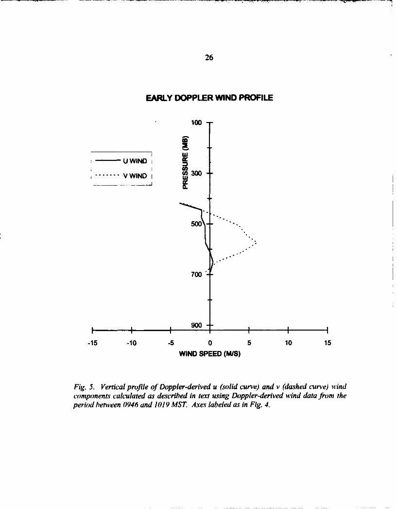
26

EARLY DOPPLER WIND PROFILE

100

w

UWINDS....... V ID•300

V VWIND I .

500

700

-15 -10 -5 0 5 10 15WIND SPEED (MIS)

Fig. 5. Vertical profile of Doppler-derived u (solid curve) and v (dashed c'urve) windcomponents calculated as described in text using Doppler-derived wind data from theperiod betiveen 0946 and 1019 MST. Axes labeled as in Fig. 4.

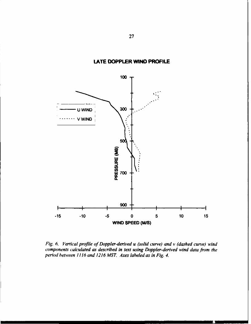
27

LATE DOPPLER WIND PROFILE

100

S....... V WIND

S0

I900-15 -10 -5 0 5 10 15

WIND SPEED (MIS)

Fig. 6. Vertical profile of Doppler-derived u (solid curve) and v (dashed curve) windcomponents calculated as described in text using Doppler-derived wind data from theperiod between / 116 and 1216 MST. Axes labeled as in Fig. 4.

28

UNSMOOTHED MODEL TERRA IN

07.5 0

*V sC) o

-2.5V

.7.

-a -17.5 -2.5 -7.5 -&S 25. 7.5 12.5 I.5 =.S

X (KM)

Fig. 7. Topographical view of terrain features near Langmuir Laboratory. Terrainelevation is relative to sea level in dekameters and contour intervals are evert' 20 deka-meters. The horizontal and vertical axes are labeled in kilometers. The origin (0,0) islocated at Langmuir Laboratory. Valleys and ridges are labeled as described in text.

29

initial activity in the mid-morning hours to full development shortly before noon to

gradual decay shortly after noon. All (xy) coordinate references are in kilometers

and based on a coordinate system with its origin at Langmuir Laboratory.

3.3.1 Pre-Storm Development

The NCAR CP-4 radar first detected an echo at 0946 MST over the eastern slope

of the main ridge approximately 1.5 km north of Langmuir Laboratory. The first

echo extended vertically to only 6.3 km MSL. The radar detected several shallow,

weak, short-lived showers between 0946 and 1110 MST. During this period one

shallow shower persisted north of Langmuir Laboratory. The shower's radar returns

rarely exceeded 40 dBZ and never extended above 6.3 km MSL. Although these ear-

ly showers never developed into thunderstorms, they served to moisten the low-level

environment for later storm development.

3.3.2 Storm Initiation And Early Development

By 1116 MST the CP-4 radar detected an organized cell (denoted hereafter as C l)

(-1.0, -4.5) with returns of approximately 20 dBZ over and east of RI south of Lang-

muir Laboratory. Cl was the first in a series of cells that developed and combined to

form a multi-cellular storm. For the purposes of this study a cell is defined, as in

Lang's (1991) analysis, as any relative reflectivity and/or updraft maximum that ex-

hibits vertical continuity. The radar also detected weak returns over R2 southeast of

the Laboratory. The radar returns at elevation 3.3 km MSL located along the main

ridge just to the north of Langmuir Laboratory appear to be ground clutter and per-

sisted through most of the remaining analysis times. By 1119 MST, Cl 's radar re-

turns (-1.0, -4.5) reached 30 dBZ, and 20 dBZ echoes extended to 7.3 km MSL. The

activity over R2 southeast of Langmuir continued to develop slowly (Fig. 8).

30

07/31/84~1119 MST 3.3 KM MSL I.O/4~ RRDARS- so s

I t :i2SP nnUW'1! I 0 ItU I

=00 3000.

11

-2 '1"1

-s ~0

-- A

-7

-10-fiin

16 ~5 -' 3 -2 1 0 1 2 3 '4 S 6 7 8

HORIZONTAL FLOW FIELD/REFLECTIVITY (OBZ)

Fig. 8. Horizontal cross-section of observed radar reflectivities in dBZ and vector v'elo-cities at an altitude of 3.3 kmn relative to mean sea level at 1119 MST 31 July 1984. Re-flectivities (solid contours) are contoured every 10 dBZ. Vector velocities areground-relative wit/h a vector length of one grid interval (0.5 kin) equal to 15 mn s-1.Terrain elevations (dashed contours) are relative to sea level in meters. and contourintervals are every 200 meters. The origin is at Lan gmuir Laboratory, and the axes arelabeled in kilometers.

31

At the next available analysis time, 1134 MST, the radar detected two well-

defined cells over the ridges: Cl (0.0, -5.0) over RI south of Langmuir; and a new

cell (denoted hereafter as C2) (2.5, -1.0) over R2 approximately 3 km east-southeast

of Langmuir. C l's radar reflectivities exceeded 40 dBZ and C2's exceeded 45 dBZ.

Cl's 20 dBZ returns extended to 9.3 km MSL, while C2's extended to 10.0 km. The

horizontal wind analysis at 3.3 km MSL showed significant upslope flow on the west-

ern side of R1 along with upslope flow through VI. The two flows converged very

near the location of Cl. Additionally, upslope flow on the eastern side of R2 con-

verged with the VI flow in the vicinity of C2. Above 6.3 km MSL, the horizontal

wind analysis also showed strong divergent flow over Cl and weak divergence over

C2 (Fig. 9). Cl contained a 1.5 km-wide updraft located on the southeastern edge of

the cell and an approximately 1.0 km-wide downdraft located just to the north of the

updraft. The updraft exceeded 9.0 m s-' between 3.3 and 6.3 km MSL with a maxi-

mum updraft of 12.0 m s-1 located at 5.3 km MSL. The updraft diminished rapidly

above 7.3 km MSL. The downdraft averaged approximately 3.0 m s- between 3.3

and 4.3 km MSL. C2 also contained a 1.5 km-wide updraft located on the southeast-

ern edge of the cell and an approximately 1.0 km-wide downdraft located north of the

updraft. The updraft exceeded 9.0 m s-1 between 5.3 and 7.3 km MSL and remained

identifiable up to 10.3 km MSL. Like Cl's downdraft, C2's extended between 3.3

and 4.3 km MSL.

3.3.3 Mature Storm Development

By 1137 MST, both Ci's and C2's maximum reflectivities exceeded 50 dBZ at

3.3 km MSL. The CP-4 radar again detected 20 dBZ returns up to 9.3 km MSL from

Cl (0.0, -4.5) and to 10.0 km MSL from C2 (2.5, -1.5). The horizontal wind analy-

sis at 3.3 km MSL showed little change from the 1134 MST analysis. The strong di-

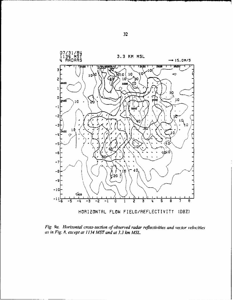
32

07/31/81411314 MST 3.3 KM MSL14 RRORRS -. 5O/

i -r- i r~io '' 2m o 00 ..,1 1 1%1 1244001 1 24A06 1 12 0 no3 10 i

to 10.. 10 .1'

11

.0........

ItC

-2I

2400

5%.J -. 0.-

-6

-100

-6 -5 -4 -3 -2 -1 0 1 2 3 4 5 6 7 e

HORIZONTAL FLOW FIELD/REFLECTIVITT (06Z)

Fig. 9a. Horizontal cross-section of observed radar reflectivities and vector velocitiesas in Fig. 8, except at 1 134 MST and at 3.3 km MRL.

33

07/31/84l134, MST 7.3 KM MSL4 RROARS -- 15.OM/S

3-

2-

1-

o-

-2-_ 2-3- "o " -/ - " - . . / y 20

-7- "2 0

-10-

11 1 1 1 1 f111 1 11 1 1 11 11 11 11 11 11

6-" -5 -4 -3 -2 -1 0 1 2 3 4 5 6 7 8

HORIZONTRL FLOW FIELD/REFLECTIVITT (OBZ)

Fig. 9b. As in Fig. 8, horizontal cross-section of observed radar refl.ctivitik ed 'ec-tor velocities for 1134 MST and at 7.3 km MSL.

34

vergence above 6.3 km MSL continued over Cl while virtually non-divergent flow

existed over C2. Cl's updraft expanded to a width of approximately 3.0 km. The

enlarged updraft contained two areas of maximum vertical velocities at low levels

which merged into a single updraft at 6.3 km. Cl's updraft exceeded 9.0 m s- be-

tween 4.3 and 7.3 km MSL with a maximum of 12.0 m s-1 between 5.3 and 6.3 km

MSL. Cl's downdraft became extremely weak (less than 3.0 m s'). C2's updraft

began to weaken considerably from the bottom with vertical velocities exceeding 9.0

m s-' only between 7.3 and 8.3 km MSL. C2's downdraft became much stronger

than at 1134 MST, exceeding 3.0 m s-1 between 3.3 and 6.3 km MSL with a maxi-

mum of 6.0 m s' at 3.3 km MSL. Strong divergent flow near 7.0 km MSL over CI

contributed to the weakening of C2's updraft.

The trend of Cl strengthening and C2 weakening continued at 1140 MST. The

radar continued to detect maximum returns of 50 dBZ from both cells, but C I's stron-

gest returns (-0.25, -4.75) extended higher (to 4.3 km MSL) than at the previous

time. Cl's double-maxima updraft continued with the northern branch strengthening

to 15.0 m s1 between 5.3 and 6.3 km MSL while the southern branch remained at

about 9.0 m s-'. The two branches merged near 8.3 km MSL. Meanwhile, C2's

(2.25, -0.75) updraft weakened to about 6.0 m s-1. Both cells contained weak down-

drafts at this analysis time. Cl's downdraft remained less than 3.0 m s1, while C2's

decreased to about 3.0 m s-1 between 3.3 and 4.3 km MSL. The vertical cross-

section shown in Figure 10 again shows strong divergent flow near 7.0 km MSL over

CI undercutting the remnants of C2's updraft.

By 1143 MST, both cells had weakened from their previous strengths. Cl's

maximum reflectivity (-0.25, -4.0) decreased to 45 dBZ and C2's (2.25, -1.75) de-

creased to 40 dBZ. The horizontal flow at 3.3 km MSL remained virtually un-

35

07/31/8q1140 MSTCROSS-SECTIONS 4 RRAR4.26KM REFLECTIVITY [OBZ)

3 10

I01 1 - o

11001

100

_ 10,x Sj 10/

10

-55

-7-2

-6 R /-q -22

Fig. lOa. Horizontal cross-section of observed radar reflectivities in dBZ at an altitudeof 4.3 km relative to mean sea level at 1140 MST 31 July 1984. Reflectivities are con-toured every 5 dBZ. The origin is at Langmuir Laboratory. The ares are labeled inkilometers. Line AB shows the location of the vertical cross-section in Fig. lOh.

36

R (0.4,-3.71 AT 57.0 OEG 11040 MST 07/31/8 BSTORM MOTION COMPONENT IN PLANE -P 20.0 M/S

Jq I I I I I I I I I I I I I I I I I i

12-

10 0

:2

- ,' e II I I II I I I I I I I Ix- s -3.7 - -2.5 -3.5 -o.11 0.7 1.3 2.9 3.9 5.0

-11.7 -10.0 -6.I -6.7 -5.0 -3.3 -. 7 0.0 1.7 3. .VELOCITY/REFLECTIV ITT

Fig. lOb. Vertical cross-section of observed radar reflectivities in dBZ and vector velo-cities at 1140 MST 31 July 1984. Reflectivities are contoured eve' 5 dBZ. Vector ve-locities are ground-relative with the vector length shown in upper right-hand corner of

figure equal to 20 m s/. Cross-section location AB is shown in Fig. IOa.

37

changed from previous times. The horizontal wind analyses between 4.3 and 5.3 km

MSL, however, showed that the circulation induced by Cl significantly diminished

the southwesterly flow into C2 found in earlier analyses at these levels. Cl's updraft

remained split with the northern branch dominant with vertical velocities exceeding

12.0 m s-1 at 7.3 km MSL. The southern branch contained vertical velocities as

strong as 9.0 m s-. Cl again developed an identifiable downdraft of about 3.0 m s-

between 3.3 and 4.3 km MSL. C2's updraft became very weak (approximately 3.0

m s-1) and narrow (approximately 0.5 km wide). C2's downdraft remained at about

3.0 m s- at 3.3 km MSL.

At 1146 MST both cells began to show some signs of regeneration. The reflecti-

vities from both cells remained about the same as at 1143 MST. The horizontal wind

analysis shows continued strong low-level convergence near the location of Cl (0.0,

-3.5) and increased low-level convergence in the vicinity of C2 (2.25, -1.25). Strong

upper-level divergence continued over CI (Fig. 11). The split updraft continued in

Cl with the northern branch remaining dominant. A new updraft formed at this time

on the eastern edge of CI (over the western slopes of R2). This updraft was approxi-

mately 1.0 km wide and reached a maximum strength of 9.0 m st before merging

with the other two branches of Cl's updraft at 8.3 km. C2's updraft remained very

narrow, but increased in strength to over 9.0 m s- between 6.3 and 8.3 km MSL with

a maximum of 12.0 m s-1 at 7.3 km MSL. Cl's downdraft remained 3.0 m sl, but

increased in vertical extent to 5.3 km MSL. C2's downdraft remained unchanged

from the previous analysis time (Fig. 12).

The regeneration trend of Cl (0.0, -4.25) continued at 1149 MST as its maximum

reflectivity increased to 50 dBZ. C2's (3.0, -1.75) maximum reflectivity remained

steady at 40 dBZ, but extended in height to 7.3 km MSL from the previously ob-

38

07/31/841146 MST 3.3 KM MSL

2~ca1 403

0P

21400

0-7

-290

-10

OF N7. aa a

-7 - 5 -'. -%- 1 0 1 2 3 '

HOI-8LFO ILORFETVT OZ

Fi. a.Hoionalcos-scio o bsredraa rflcivtisan vcorveoiteas~~~~~~~~~~; inFg ,ecp t146MTada . mML

39

07/31/85411146 MST 9.3 KM MSL4, RRORRS 15.0 M/S

SI I I I I I I I I "I I I I I I I I I I I I I ! I I I I

3-

2-11 '10

0 - • , I i,

-2- 1 - - - - - - --

_L . 3G"1 .-2D-20

--5 -- - - - - --

10 .110

-110

t I im

10 10 Ud'*l 0,

- 8 0

- 6 -5 -'1 -3 -2 -1 0 1 2 3 4 5 6 7 8

HORIZONTRL FLOW FIELD/REFLECTIVITT (DBZ)

Fig. I lb. As in Fig. 8, horizontal cross-section of observed radar reflectivities and vec-tor velocities for 1146 MST and at 9.3 /In MSL.

40

07/31/84111146 MST 3.3 KM MSL41 RADARS

I I I I I I I I I I I I I I I I I I I I I I I I I I

3

2

1

0-

-1

-2-

-33

-5 •O

-6

-7-

-81

0-10

I I I I I 1 I I I I I I III I I I I I I I I I I I I I

-6 -S -q -3 -2 -1 0 1 2 3 4 5 6 7 8

W COMPONENT (M/S)

Fig. 12a. Horizontal cross-section of observed vertical velocities at an altitude of 3.3km relative to mean sea level at 1146 MST 31 July 1984. Velocities are contoured ev-ery 3.0 m s-i starting at 0 m sl. Solid contours denote upward vertical velocities(positive w). and dashed contours denote downward vertical velocities (negative w).Origin and axes are as in Fig. 8.

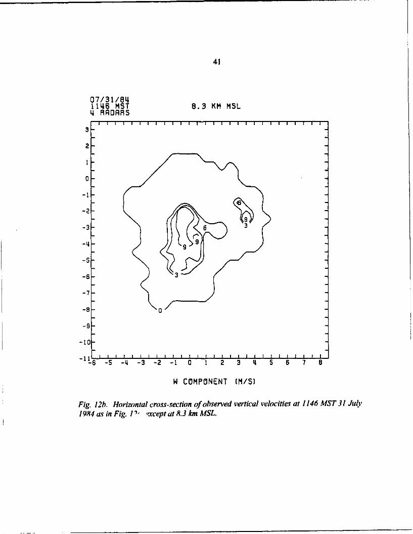
41

07/31/841146 MST 8.3 KM MSL4 RADARS

3-

2-

0-

2-

-3

-4-

-6E

-7-

-91-

-10_

i i i i I I , t I l I IlI I I I I I , I I I I I I I

-6 -5 -4 -3 -2 -1 0 1 2 3 4 5 6 7 8

W COMPONENT (M/S)

Fig. 1 2h. Horizontal cross-section of observed vertical velocities at 1146 MST 31 July1984 as in Fig. I" except at 8.3 km MSL.

42

served 3.3 km MSL. Low-level convergence continued in the vicinity of C I and C2,

while strong divergence continued over Cl. The reflectivity analysis also shows the

development of a new cell (-0.5, -7.5) (denoted hereafter as C3) as an elongation in

the reflectivity contours along Rl's ridge axis (Fig. 13). Cl's updraft remained split

at this time. The new updraft noted on the eastern edge of cell CI at 1146 MST

dominated Cl with a maximum vertical velocity of 18.0 m sl at 6.3 km MSL (1.25,

-4.0). Cl's southern updraft remained relatively strong with a maximum updraft of

12.0 m s-' (0.0, -5.5). The two updrafts merged with each other and with the rem-

nants of the older third updraft at 8.3 km MSL. C2's updraft (3.25. -2.5) remained

relatively weak, barely reaching 9.0 m s1 at 8.3 km MSL. C3 contained no distin-

guishable updrafts or downdrafts at this time. The downdrafts from both Cl and C2

combined to form a broad area of downward motion covering approximately 12 km2

below 4.3 km MSL northwest of the updrafts. The downdrafts reached a maximum

strength of 6.0 m s1 (Fig. 14).

By 1152 MST, Cl (-0.25, -4.0) had drifted slowly northward. C2 lost its identity

after slowly weakening and being absorbed by the northward-moving Cl. Cl re-

mained strong with its maximum reflectivity exceeding 50 dBZ. C3 (-0.25, -6.5)

showed further signs of development with its maximum reflectivity exceeding 30 dBZ

between 3.3 and 8.3 km MSL. The horizontal wind analysis continued to show

strong convergence over both RI and R2, especially at 4.3 km MSL. Strong diver-

gence existed above both C1 and C3 at and above 8.3 km MSL. Cl continued with a

very complex updraft structure below 8.3 km MSL. Several small updrafts formed at

this time below 8.3 km MSL, especially along the southeastern edge of the cell.

These were likely caused by the convergence of the downdraft air as it spilled down

the valleys and the southeasterly flow up the valleys ahead of the storm. The updrafts

43

07/31/8411149 MST 7.3 KM MSL14 RORRS -- 15.O4/5

I I I I I I I I I I 1 I ! I I I | I ! I I ! I I I

3-

2-

I - - "010I 4

0-

-10

-2

-7

-8-1 20

-39

-10- --

-5 -41 -3 -2 -1 0 1 2 3 q 5 6 7 8

HORIZONTRL FLOW FIELD/REFLECTIVITT (DBZ)

Fig. 13. As in Fig. 8, horizontal cross-section of observed radar reflectivities and vec-tor velocities for 1149 MST and at 7.3 km MSL.

44

07/31/8u411'49 MST 3.3 KM MSL4. RORAS

I I I I I I I I I I I I I I i I I I I I I I I I I I

3-

2- 0

0-

-3-7-

---

-7-

-10-

- I I I I I I II I I I I I I I I II I I I I

- -5 -' -3 -2 -1 0 1 2 3 4 5 6 7 8

W COMPONENT (MIS)

Fig. 14a. Horizontal cross-section of observed vertical velocities as in Fig. 12a. exceptat 1)49 MST and at 3.3 km MSL. Labels indicate locations of updrafts associated with

ells Cl and C2.

45

07/31/•411'49 MST 6.3 KM MSL'4 RADARS

S I I I i I I I I I I i I i I III I I I I I I I I I I

3

2-

0- .

-24--

-3-

-7'- 0

-5j0

-to

-I I I I I I I --5 -4 -3 -2 -1 0 1 2 3 4 5 6 7 8

W COMPONENT (M/S]

Fig. 14b. As in Fig. 12a, horizontal cross-section of observed vertical velocities.fi•r1149 MST and at 6.3 km MSL. Labels indicate locations of updrafts associated withcells Cl and C2.

46

combined to form the main CI updraft with a maximum strength of 12.0 m s-1. CYs

narrow updraft (approximately 0.5 km wide) strengthened markedly from the pre-

vious analysis to a maximum strength of 15.0 m s-. Cl's downdraft continued to

cover a broad area with a maximum strength of 6.0 m s-'. The vertical cross-sections

shown in Figure 15 show that CI had a significant backward tilt. As a result, the pre-

cipitation and the precipitation-induced downdraft occurred north and west of the up-

draft so that they did not interfere with it. Similar storm structures and circulations

have been observed in some long-lived severe storms (see e.g., Browning et al.,

1976).

Poor data quality at 1155 MST prevented an analysis for that time. At 1158

MST, Cl (0.5, -3.5) reached its peak intensity, and C3 (-0.5, -6.5) increased in

strength slightly. Cl's area of 50 dBZ reflectivities grew substantially from 1152

MST, and C3's reflectivities increased to 40 dBZ. A new cell (5.0, -3.5) (denoted

hereafter as C4) developed at this time over R3 (Fig. 16). The maximum reflectivity

from C4 reached 40 dBZ at 7.3 km MSL. Strong low-level convergence continued

over both RI and R2. The horizontal wind analysis showed strong divergence over

C1 between 10.3 and 12.3 km MSL and over C3 and C4 at 8.3 km MSL. Cl's mul-

tiple updrafts continued, but weakened considerably at low levels. The analysis

showed updrafts greater than 9.0 m s-1 only above 8.3 km MSL with maximum up-

drafts of 12.0 m s-. The updrafts merged at 11.3 km MSL. The downdraft asso-

ciated with Cl became very broad and strong by this time, exceeding 12.0 m sl at

3.3 km MSL. The downdraft impacted the surface very near the top of Vl. The

analysis also showed a strong updraft (maximum strength 18.0 m s-') associated with

C3 located directly over RI. The vertical cross-sections shown in Figure 17 show the

strong interrelationships between the circulations of all three cells. For example, the

47

07/31/841152 MSTCROSS-SECTI ONS L RAROAR't.26KM REFLECTIVIT (OBZ)

Is

-to

I04 to /I

0\5 5 lo

-9 -- 10 010

-- 6 -q -2 02

A

Fig. 15a. Horizontal cross-section of observed radar reflectivities as in Fig. lOa. ex-cept at 1152 MST and 4.3 km MSL. Lines AB and CD show locations of'vertical cross-sections in Figs. 15b and l5c. respectively.

48

R C-0.3.-3.7) AT 90.0 DEG 1152 MST 07/31/84ASTORM MOTION CMOETIN PLANE -p20.0 NIS

12-

10-a ,-

y -13.3 -11.3 -9.3 -7.3 -5.3 -3.3 1*3 0.8 2.8 4:8

VELOCITT/REFLECrI VITY

Fig. l~b. As in Fig. 10b, vertical cross-section of observed radar reflectivities and vev-for velocities at 1152 MST. Cross-section location A B is shown in Fig. 15a.

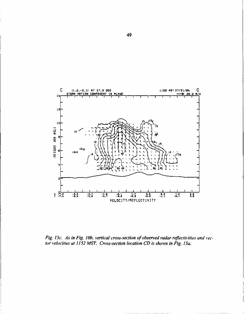
49

C (1.2.-3.1) AT 27.0 DEG I1152 MST 07/31/8's 0STORM MOTION COMPONENT IN PL ANE 0 0. MIS

12-

10-i-is

zaa

I S.I

X 972 5.I-.7 -1. %01 17 35 . ..

-7.4 f6. -Is-. 36 -. -. 11 -. .

L 15T/~FLCIVT

Fig 1c. s n Fg.l~b vrtialcros-ecionofobsrvd rda reletivtis ad3ect()r ekwites a I 1S MS3 Crs-eton' loainC 2ssoni i.I

50

07/31/8B41158 MST 8.3 KM MSL4 RFRORAS -- 15.OM/S

I I I I I I I I I I i I I I I I I I I I I I I I I I | I

3 - 1010

2

1 10

-3- -5 -4 -- -2 -- 0 1 2 - - -

5 -- P2

a t dt-L• • • • - • 10

- . . . . .-. 9 - 2-. . .

- -5. . .- . .2 - 0 1 2 3 q 5 6 7 8

HOFRIZONTFIL FLOW FIELD/FREFLECTIVITT [DBZ)

Fig. 16. Horizontal cross-section of observed radar reflectivities and vector velocitiesas in Fig. 8, except at 1/158 MST and at 8.3 Ian MSR.

51

07/31/841158 MST '

CROSS-SECT IONS ROR,4.26KM REFLECTIVITY (OBZ)

S101_

C 0 0-1 -0

iis

1 1 5

A I -2 0 2 5

Fig. 17a. As in Fig. 1Oa, horizontal cross-section of observed radar reflectivities at1158 MST and 4.3 km MSL. Lines AB and CD show locations of vertical cross-sectionsin Figs. 1 7h and 1 7c, respectively.

52

R (0.5,-3.61 AT 56.0 OG 1158 MST 07/31/811STORM NOTION COMPONENT IN PLANE b 20.0 M/SI1 I I I I I I I I I I I I I I I I I

12-

Is -

I-I

IS/ 10 IO_

10- 1 !

I:Is.

I I I I I I I l I I I I I I I I Ix 1.4 -2.0 -1.7 -0.9 -.0.I 0.7 I.S 2.3 3.1 4.0T -12:3 -ta.5 -0.3 -6.0 -5.0 -3.1 -1.3 O.S 2.3 '8.2

VELOCITY/REFLECTIVITY

Fig. 17b. Vertical cross-section of observed radar reflectivities and vector velocities asin Fig. lob, except at 1158 MST. Cross-section location AB is shown in Fig. 17a.

53

C (0.3.-2.s5 AT -5.0 OEG 1158 MST 07/31/$q 0STORM MOTION COMPONENT IN PLANE b 20.0 M/Sti I I I ! II I I I I I I I I I I !

12-

-10

x -. 2 -7.2 -5. 2 -3.2 -1.2 0.7 2.7 3.7 6.7 6.7T -1.7 -1.8 -2.0 -2.2 -2.: -2.5 -2.7 -2.9 -3.1 -3.2

VELOC I TT/REFLECTIV ITT

Fig. 17c. Vertical cross-section of observed radar reflectivities and vector velocities asin Fig. lob, except at 1158 MfST. Cross-section location CD is shown in Fig. / 7a.

54

outflow at the top of C3, the newer cell, feeds directly into the much higher updraft

in the older cell, Cl. Additionally, the flow through C4 feeds directly into Cl's up-

draft.

3.3.4 Storm Decay

The 1201 MST analysis suffered from a lack of data over most of the southern

half of the analysis grid. The available data showed CI (0.5, -3.0) began a slight

weakening trend at this time. The maximum reflectivities observed from Cl de-

creased to 40 dBZ. C3 (-0.5, -6.5) moved slightly northward and weakened slightly.

but radar still detected 45 dBZ returns. The actual amount of weakening is question-

able due to the lack of data. C4 (5.0, -3.0) continued to strengthen with 40 dBZ re-

turns detected between 6.0 and 8.3 km MSL. The horizontal wind analysis showed

strong mid-level divergence southeast of the storm area over the eastern slope of RI.

Additionally, the analysis showed strong upper-level divergence over both C I and C3.

The updrafts in both C I and C3 weakened at this time: C I to a maximum strength of

9.0 m sl, C3 to a maximum of 12.0 m s-'. C4's updraft intensified rapidly to 12.0

m s-1. Cl's downdraft remained broad and strong with a maximum strength of 12.0

m s" at 3.3 km MSL. The missing data prevented analysis of C3's downdrafts. C4's

rapid intensification led to the development of a narrow, but strong downdraft (9.0

m s-1).

The reflectivity analysis at 1204 MST showed only minor changes in Cl (0.5,

-2.5) and C3 (0.0, -5.5) from the 1201 analysis. By 1204, C4 (3.5, -2.5) had drifted

northwestward to the location where C2 had previously dissipated, and its area of 40

dBZ returns extended downward to 3.3 km MSL. The radar detected 30 dBZ returns

between 4.3 and 7.3 km MSL from a new cell (-4.0, -5.0) (denoted hereafter as C5)

just west of RI (Fig. 18). The horizontal wind analysis showed a weakening of the

55

07/31/841204` MST 6.3 KM MSL4L RADARS -1 1S.OM/S

31- l 1llOio 1 1110 12 orr r

-•n 10102 0 10 10

10

0 " 10

-10

115 . . ..- -3 .2 - 0 1-2.3 4.5,6,, .-or-eltiesfo 10 MT a t 6 •

21 40!

-6" -5 -q -3 -2 -1 0 1 2 :3 4 5 6 7 8

HORIZONTRL FLOW FIELD/REFLECTIVITY (DBZ3

Fig. 18. As in Fig. 8, horizontal cross-section of observed radar reflectivities and 1ec-tor velocities for 1204 MST and at 6.3 km MSL.

56

channelling effect in VI with a slight increase in the convergent channelling in V2.

Moderate low-level convergence existed in the region between Cl and C4 directly

over the southern tip of R2. The mid-level divergence continued over the eastern

slopes of RI and a new divergence area formed over the western slopes of RI in the

vicinity of C5. The strongest upper-level divergence existed over C4. The vertical

velocity analysis for 1204 MST showed a slight increase in updraft strength in Cl,

C3, and C4. The analysis showed no distinct updraft regions associated with C5.

The downdrafts in CI and C4 weakened to 6.0 m s-1 and covered a slightly smaller

area than earlier. The analysis showed a well-established (6.0 m s-1) downdraft asso-

ciated with C3. The vertical cross-section (Fig. 19) shows the strong development of

C4 and that its circulation continued to feed into Cl's circulation.

The reflectivity analysis at 1207 MST showed very few changes from the 1204

and 1201 MST analyses. By this time both CI (0.5, -2.5) and C3 (0.0, -5.5) had

drifted slowly northward. Radar detected several new echoes developing over the

eastern slopes of R3. These appear to have developed as a result of the strong ups-

lope flow into C4 (3.5, -2.5). The horizontal wind analysis showed continued strong

low- and mid-level convergence in the vicinity of C1. The analysis showed strong

upper-level divergence over both C3 and C4. Cl's updraft remained at about the

same strength as at 1201, while C3's weakened slightly. C4's updraft weakened con-

siderably to a strength of 6.0 m s-. C5's (-3.75, -4.75) updraft became more orga-

nized, reaching a strength of 6.0 m s-'. All four active cells showed organized

downdrafts at this time with Cl's and C3's increasing in strength again to over 9.0

m s-'. The vertical velocity analyses showed that by this time the updrafts existed

mainly at mid- and upper-levels.

57

07/31/841204 MSTCROSS-SECT IONS 4 RADR4.26KM REFLECTIVITY' (oez]

Fg 1 1a. sinFg ia I

19b. Ln ABwa nt•oued

0 is 101

-t 0120 0 is2301002Fig 19. A inFig l~, hriznta crss-eto fosre aa elciiisa

Fi.19a. AsT ind Fi.3 10a hor.iznt Dsoslcto fvral cross-section ofosre aa elcinii it.

19h. Line ,AB was not used.

58

C (1.2.-2.1) AT -14.0 OEG 120q MST 07/31/84 0STORM MOTION COMPONENT IN PLANE b 20.0 MIS

l•--12

10- I-t

x -8.0 -'4. 1 -2.1 -0.2 1.7 3.7 5.8 7.8 9.57r 0.2 -0., -0.S -4.3 -1.7 -2.2 -2.7 -3.2 -3.7 -'1.2

VLOC ITT/4 FLCT IV I2TT

Fig. 1 9b. Vertical cross-section of observed radar reflectivities and vector velocities asin Fig. l Ob, except at 1204 MST. Cross-section location CD is shown in Fig. / 9a.

59

By 1210 MST, the defining reflectivity contours of Cl (0.5, -2.0) and C3 (0.5,

-4.5) had merged. Radar returns from C4 (3.0, -2.5) weakened slightly while those

from C5 (-3.5, -4.0) increased in strength to 40 dBZ at 3.3 krn MSL. The weak de-

velopment over R3 continued while several new cells formed in the extreme north-

eastern corner of the analysis area. The horizontal wind analysis showed strong

low-level convergence over the western slopes of R2 and over the northern end of V2.

Strong upper-level divergence also existed over these same regions. Cl's updraft re-

mained as its oni distinguishing feature at 1210 MST. At this time, it still main-

tained a strength of 9.0 m s-'. C3's updraft remained about the same strength as at

1207 MST, but C4's updraft strengthened again to 9.0 m s-1. and C5's updraft

reached 9.0 m s- for the first time. At this analysis time, Cl's downdraft had de-

creased significantly to less than 3.0 m s'. C3, C4, and C5 all contained maximum

downdrafts of 6.0 m s-1.

By 1213 MST, C3 (0.5, -3.5) had overtaken all remnants of Cl and most of the

remnants of C4 (2.5, -2.0). C3's maximum reflectivity increased to over 50 dBZ at

3.3 km MSL at approximately the midpoint between the previous locations of C3,

C l, and C4. C4 appeared in the reflectivity analysis as only a bulge in the 40 dBZ

contour at 3.3 kln MSL. C5's (-3.0, -4.0) maximum reflectivity remained about 40

dBZ, however the maximum expanded in vertical extent to 5.3 km MSL. A new cell

(2.0, -7.0) (denoted hereafter as C6) developed along the southeastern edge of C3 al-

most directly over the center of VI. This cell was best defined in the reflectivity

analyses at 6.3 and 7.3 km MSL (Fig. 20). The horizontal wind analysis showed

weak low-level flow over the northern half of the analysis domain, but a relatively

strong southwesterly flow over the southern half. The analysis showed very little

low-level convergence. Some upper-level divergence still existed over C3 and C6.

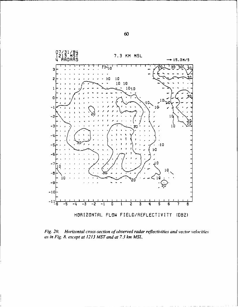
60

07/31/8141213 MST 7.3 KM MSL'4 ARORAS - 5O/

3 . . . . .

2~~~ ~ ~ ~ .. . ..... -1

-10-10 '

HOI0NR FLWFEO0ELC ,VT DZ

Fig. ~ ~ ~ ~ ~ ~ ~ ~ -20. Hoiotlcosscinofosre-aaoelciite n etrvlcte

as n Fg.8, xcpt t 213M0 n t . mML

61

C3's updraft continued with a maximum strength of 9.0 m s' between 5.3 and 9.3 km

MSL while C4's updraft became indistinguishable at this time. C5's updraft contin-

ued to strengthen, reaching a maximum strength of 12.0 m s-'. By 1213 MST, C6's

updraft had already reached 9.0 m s-I between 5.3 and 6.3 km MSL. The area cov-

ered by C3's downdraft continued to shrink, although the downdraft's maximum

strength continued at 6.0 m sl. The weak downdraft (3.0 m sl) remained as the only

structure that distinguished C4 from C3 at 1213 MST. C5's downdraft increased in

strength to 6.0 m s'.

At 1216 MST, C3 (0.5, -4.0) had absorbed the final remnants of C4. C3 contin-

ued with a maximum reflectivity of 40 dBZ. C5 (-3.0, -4.0) maintained its previous

strength, while C6 (2.0, -7.0) strengthened rapidly, with its 40 dBZ maximum reflec-

tivities extending down to the lowest analysis level of 3.3 km MSL. A weak new cell

(5.5, -2.0) (denoted hereafter as C7) developed at this time over R3. The horizontal

wind analysis at this time again showed very weak flow over the northern half of the

analysis domain with a relatively strong southerly to southwesterly flow over the

southern half. Some weak low-level convergence existed just east of C6. The verti-

cal velocity analysis showed that by this time most of the vertical motion had weak-

ened considerably. Only C6's updraft exceeded 9.0 m s-. Downdrafts of 6.0 m s-

existed only in C3 and C5 by this time.

3.3.5 Summary

The previous subsections provide a detailed description of the initiation and evolu-

tion of the 31 July 1984 storms as observed by the Doppler radars. These observa-

tions provide some insight into the general nature of the storms.

Early cell development occurred directly over or slightly east of the ridge lines.

These observations are consistent with the theory that the New Mexico storms evolve

62

mainly as a result of thermally driven mountain-valley circulations and are focused by

local topographic features (see, for example, Barker and Banta, 1985; Banta and

Schaaf, 1987; Schaaf et al., 1988). The weak low-level southeasterly flow into the

convergent valleys, V I and V2, produced areas of upslope and convergent flow at the

northwestern (upslope) end of those valleys. The upslope flow and convergence fo-

cused the areas of convective initiation over the ridges nearest the ends of VI and V2

as described by Banta and Schaaf (1987).

After the first cells had developed, the mountain-valley circulation and the conver-

gent flows continued to help focus the location of new cell initiation. However, cir-

culations from the existing cells also began to affect the location of cell initiation.

For example, at 1152 MST, several short-lived cells developed along the outflow

boundaries from Cl and C3. In some cases the low-level flow induced by the exist-

ing cells enhanced or created upslope and/or convergent flows which in turn helped

focus new cell development.

The storm observed near Langmuir Laboratory on 31 July 1984 generally had a

lifetime of approximately 1.0 to 1.5 hr. The storm contained several cells with life-

times of from 20 to 60 min. Many of the cells exhibited periodic intensification and

weakening with a period of 6 to 12 min. For example, both CI and C2 underwent at

least two cycles of intensification/weakening during the analysis period (CI from

1134 to 1143 MST and 1146 to 1210 MST; C2 from before 1134 to 1143 MST and

1146 to 1152 MST). This periodic activity resembles closely the updraft pulsations

suggested by Ziegler et al. (1986). Radar returns from the strongest cells exceeded 50

dBZ several times, but maximum returns from most cells ranged from 30 to 40 dBZ.

Most of the cells never extended higher than 10.0 km MSL, however, the stronger

63

cells, CI and C4, frequently extended above 10.0 km and in some cases to over 12.0

km MSL.

Most cells contained single updrafts approximately 2.0 km wide with maximum

vertical velocities of 12.0 m s- or less. Cl frequently contained multiple low-level

updrafts which merged into a single updraft at mid-levels. The strongest observed

updrafts of 18.0 m s-1 occurred in C1 and C3. In the early stages of cell develop-

ment, the downdrafts were only about 1.5 km wide with maximum vertical velocities

of 3.0 m s- or less. As the cells matured, however, the downdrafts expanded in areal

coverage and increased in strength with maximum vertical velocities frequently ex-

ceeding 6.0 m s-1 and with an absolute maximum of 12.0 m s1. In at least one cell,

Cl, during the cell's mature stage, the interaction between the updraft and the down-

draft appeared to be symbiotic in a manner similar to that often observed in long-lived

severe storms. As discussed in a previous section, the updraft tilted northwestward

(or backward relative to the low-level storm inflow). The precipitation and its asso-

ciated downdraft were located behind and below the updraft (relative to the low-level

inflow) and thus did not interfere with the inflow or the updraft. Several other cells

contained tilted updrafts, but to a lesser extent than Cl. As the cells entered the

decay stage, the updrafts became nearly vertical so that the precipitation and the

downdraft interfered considerably with the updraft.

The Doppler radar observations and the associated wind analyses reveal a strong

interrelationship between all the cells in the analysis domain. Ia the mature stage, the

outflow from downdrafts appeared in some cases to enhance low-level convergence

that either focused the development of new cells or helped sustain existing cells. In

several instances the updrafts of two or more cells merged into one updraft at upper-

levels. Often the updraft of a newer cell developed in the low- to mid-levels and fed

64

into a higher-level updraft associated with an older cell. Additionally, the divergent

flow located near the top of a strong cell often cut off the updraft of a weaker neigh-

boring cell. The periodic intensification noted above frequently appeared to alternate

among the cells. For example, during Cl's first period of intensification, C2 was

weakening. This certainly did not occur without exception, but the trend was readily

apparent. Finally, the observations showed several cases where older or weaker cells

were overtaken and absorbed by newer and/or stronger cells.

Chapter 4

The Numerical Model

This chapter describes the numerical model chosen for this study. Section 4.1 de-

scribes the criteria used to select the numerical model. Section 4.2 discusses the mod-

el's ability to simulate mountain thunderstorms. In section 4.3 the model selected for

this study is briefly described. Sections 4.4 and 4.5 describe the model's vertical and

horizontal grid structures, respectively, and section 4.6 describes the topography used

in the numerical simulations. Finally, the model initialization procedure is discussed

in section 4.7.

4.1 Model Selection

Before conducting any numerical study, a numerical model must be selected.

Choosing a model is extremely important and should be deliberate and well-planned.

Essential criteria must be defined and used in the selection process. Flexibility, appli-

cability, and availability must also be considered. If existing models do not meet the

needs of the study, then a new model must be developed.

To study the type of mountain thunderstorms of interest here, it was necessary to

choose a model with fully compressible, non-hydrostatic equations of motion; the op-

tion of conducting two- or three-dimensional simulations; a terrain-following coordi-

nate system; a surface layer parameterization and a soil model which interact with

realistic long- and short-wave radiation parameterizations; and a cloud microphysical

parameterization which includes the ice phase. Additionally, the model needed to be

compatible with locally available computer software and hardware. The Colorado

65

66

State University (CSU) Regional Atmospheric Modeling System (RAMS) was chosen

for this study. RAMS was chosen over other potential models because it met all of

the above criteria, because of its flexibility, its applicability to modeling mountain

circulations and storms, and its availability.

4.2 Model Ability To Simulate Mountain Storms

Before undertaking any numerical study, it is essential to assess the model's ability

to simulate the basic processes responsible for the phenomenon under study. This

study is concerned with the initiation and development of mountain thunderstorms un-

der conditions of strong solar heating and weak ambient flow. As discussed in Chap-

ter 3, the-.-- processes are expected to include primarily thermodynamic processes and

possibly dynamic processes such as orographic lifting and valley channeling. Only

after verifying the model's skill with these processes can we use it with confidence to

study the more complex phenomenon of mountain thunderstorms.

The simple, three-dimensional, no-wind simulation used by Klemp and Wilhelm-

son (1978a) to test their model also provided an excellent test for this model's skill

with thermodynamic processes. In this test, simulated convection is initiated by in-

serting a warm, moist, symmetric perturbation in the lower part of an otherwise ho-

mogeneous atmosphere. Because this type of perturbation should yield an

axisymmetric storm, this type of test can immediately reveal many coding errors.

This was an important benefit in this case because RAMS was revised and recoded

shortly before the start of this study. The results of this test did, in fact, reveal sever-

al coding errors. After these errors were corrected, the test results agreed very well

with those reported by Klemp and Wilhelmson. Some minor differences were noted

between the two tests. These could be attributed to the different physical parameter-

izations used by the two models. Tripoli (1986) tested the model's ability to simulate

67

simple gravity waves and reported good agreement between his simulations and those

of Durran (1981).

In addition to these simple tests, the model has been used for simulations of more

complex processes important to mountain convection. Banta (1983, 1986), Bader and

McKee (1983, 1985), and Bader et al. (1987) used the cloud model portion of RAMS

to study mountain upslope flow and boundary layer evolution. Cotton and Tripoli

(1978), Tripoli and Cotton (1980, 1982, 1986), and Cotton et al. (1982) also used the

cloud model portion of RAMS successfully in studies of cumulus and thunderstorm

development. The simple Klemp-Wilhelmson tests described above, along with the

successful complex simulations carried out by other investigators, indicate that the

model is well-suited to simulate the initiation and development of mountain thunder-

storms of interest in this study.

4.3 Model Description

As its name implies, the CSU RAMS is a modeling system, not a single model.

RAMS is a combination of the Tripoli and Cotton (1982) non-hydrostatic cloud model

and of two hydrostatic mesoscale models (Tremback et at., 1985; Mahrer and Pielke,

1977). Because of this combination, RAMS is very flexible and allows the user to

select from a wide variety of physical processes and numerical techniques.

This study employed the non-hydrostatic cloud model portion of RAMS. This

section briefly describes the characteristics of the non-hydrostatic model and the vari-

ous options employed in this study. The description here closely follows that given by

Tripoli (1986).

The model formulation is a revised and slightly modified form of the CSU

cloud/mesoscale model described by Tripoli and Cotton (1982) and Cotton et al.

(1982, 1986). The model employs a non-hydrostatic, quasi-Boussinesq, fully com-

68

pressible set of primitive equations cast in two or three dimensions (Tripoli and Cot-

ton, 1986; Tripoli, 1986). The current model formulation follows Klemp and

Wilhelmson (1978a) and predicts the Exner function (x) and diagnoses density

(Tripoli, 1986; Bader et al., 1987).

The model uses time-dependent partial differential equations to predict the three

wind components (u, v, w), the Exner function (x) , the liquid-ice potential tempera-

ture (0,) (Tripoli and Cotton, 1981), total water mixing ratio (r, ), mixing ratios of

rain water (r,), pristine ice crystals (ri ), graupel or hail (rg), and aggregated snow

flakes (r,,). The model also predicts the total concentration of pristine ice crystals

(Nk,). This gives a total of eleven prognostic variables. The model uses a diagnostic

procedure described by Tripoli and Cotton (1982) to diagnose potential temperature

(0), temperature (T), cloud water mixing ratio (r,), water vapor mixing ratio (r),

pressure (p), and density (p).

The model includes parameterizations for several important physical processes.

Microphysical processes are treated by a generalized microphysical parameterization

scheme described by Tripoli et al. (1988). Within this generalized framework it is

possible to vary parameters to formulate the desired microphysical parameterization.

The microphysical parameterizations chosen for this study are similar to those of

Tripoli and Cotton (1980) for warm rain processes and Cotton et al. (1982, 1986) for

ice phase processes. Long- and short-wave radiative tendencies on 0il are computed

following Chen and Cotton (1983). For the simulations conducted in this study, the

radiative tendencies were updated at 120 s intervals starting at t = 900 s. Surface

layer fluxes of heat, moisture, and momentum are parameterized following the meth-

ods of Louis (1979) and Manton and Cotton (1977). A surface roughness of 1.0 cm

was prescribed for the surface layer parameterization. Soil temperature and soil mois-

69

ture are predicted by an underlying soil model described by McCumber and Pielke

(1981) and modified by Tremback and Kessler (1985). The soil model included five

levels located at the surface and 1, 4, 16, and 32 cm beneath the surface. Chapter 5

provides further details on the soil parameters prescribed for the simulations. Turbu-

lent mixing abovr the surface layer is modeled using the eddy viscosity approach de-

scribed by Lilly (1962). Mixing is enhanced in unstable regions as suggested by Hill

(1974) and implemented by Tripoli (1986).

The predictive equations are solved on a staggered grid described by Tripoli and

Cotton (1982) with a terrain-following vertical coordinate system similar to that of

Gal-Chen and Sommerville (1975a, 1975b). The time-differencing scheme used here

was described by Tripoli and Cotton (1982) and modified by Tripoli (1986). The

time-split leapfrog scheme developed by Klemp and Wilhelmson (1978a) provides the

basic time-differencing framework. In this scheme the terms responsible for sound

wave propagation are integrated on a small time step while the non-acoustic terms are

held fixed for several small time steps and updated on the larger leapfrog time step.

For the small time step, the model employs a forward-backward differencing scheme

for the horizontal terms and an implicit Crank-Nicholson scheme described by Durran

(1981) and Tripoli and Cotton (1986) for the vertical terms. The physical parameter-

izations are all computed with a forward time-differencing scheme. The turbulent

mixing parameterization uses a combined forward and Crank-Nicholson scheme sug-

gested by Paegle et aL. (1976). For this study, the acoustic terms were integrated us-

ing a 2.5 s small timestep, while the non-acoustic terms were integrated with a 5.0 s

large timestep. All advective terms are computed with a fourth-order finite-

differencing method.

70

Because RAMS is a limited area model, appropriate boundary conditions must be

specified in order to determine unique solutions to the time dependent equations. For

the top boundary condition a rigid upper lid similar to that employed by Klemp and

Wilhelmson (1978a) was used. The bottom boundary condition assumed zero mean

vertical fluxes at the surface with surface layer turbulent fluxes of momentum, heat,

and water vapor diagnosed by the surface layer parameterization. The open lateral

boundary conditions described by Klemp and Wilhelmson (1978a) were employed

with a specified intrinsic gravity wave phase velocity of 30 m s'.

4.4 Horizontal Grid Structure

The horizontal grid structure for this study was chosen to maximize the horizontal

resolution over a model domain large enough to accommodate the simulation of

mountain convection while minimizing artificial model boundary effects on the simu-

lated storms. Computational limitations dictated the choice of a medium-sized do-

main to allow for a desired high-resolution grid structure.

As discussed in Chapter 3, the storms of interest here developed over the Magda-

lena Mountains, a range that extends approximately 28 km in the north-south direction

and approximately 20 km in the east-west direction. Most of the convection on 31

July 1984 developed and remained near the center of the range. A 33 km model do-

main centered on the Langmuir Laboratory was chosen for the simulations in this

study. This domain was large enough to allow ample room for storm development

near the domain center and also provided for "buffer" regions around the domain

boundaries to minimize the boundary -ffects on the domain's interior.

A 500 m horizonta .,:solution was chosen for this study. This resolution was cho-

sen based on three considerations. First, an accurate numerical simulation of the

types of storms of interest here required a high-resolution grid to capture the cloud-

71

and sub-cloud-scale processes known to be important in mountain convection. Se-

cond, the extremely rough terrain in the model domain (see Section 4.6) necessitated

a high-resolution grid to capture the important terrain features and resultant effects on

storm development. Finally, the desire for the highest resolution possible was neces-

sarily tempered by the availability of computer resources. The 500 m grid structure

provided a suitable compromise among the considerations above.

Several other studies have employed similar grid structures and domain sizes to

simulate thunderstorm development in general and mountain convection in particular.

For example, Klemp and Wilhelmson (1978a) employed a 24 km domain with 1000

m grid spacing to simulate a generic severe storm; Tripoli and Cotton (1980) used a

35.25 km domain with 750 m grid spacing to simulate a Florida thunderstorm; and

Clark and Gall (1982) and Smolarkiewicz and Clark (1985) used a 51 km domain

with 1000 m grid spacing to simulate New Mexico and Montana thunderstorms, re-

spectively.

4.5 Vertical Grid Structure

The vertical grid structure chosen for this study reflects an attempt to adequately

resolve most of the important features of thunderstorm initiation and development

with a minimum of comput;.,r resources. It was computationally prohibitive to use an

extremely high-resolution vertical grid structure required to resolve such important

processes as turbulent fluxes, gust fronts, etc. Instead, a vertical grid structure was

chosen which resolves the processes thought to be most important and at least allows a

gross parameterization of the unresolvable processes.

Banta (1984). Braham and Draginis (1960), Orville (1965a), and others have

shown that shallow mountain-valley circulations play a critical role in he develop-

ment of mountain storms. These flows typically are only a few hundred meters deep.

72

Properly resolving such circulations would require a vertical grid spacing of 100-200

m. Tripoli (1986) showed that a grid spacing of 500-1000 m is required to adequately

resolve gravity waves under conditions similar to those ooserved over the Magdalena

Mountains. Resolving turbulent effects would require a grid spacing on the order of

tens of meters.

It is reasonable to expect the actual and simulated thunderstorms to occasionally

penetrate the tropopause. To adequately simulate this phenomenon, the model's verti-

cal domain should extend at least several kilometers into the stratosphere. The tropo-

pause on 31 July 1984 was located at approximately 12.4 km. The desired vertical

resolution of 100 m would require a computationally prohibitive 160 vertical grid

points. In order to facilitate the desired horizontal resolution of 500 m, a vertical

resolution of 500 m was chosen. Above the tropopause, the grid is stretched to a

maximum spacing of 2000 m at the top to provide the desired extension into the

stratosphere. The complete vertical grid structure (for the vertical velocity portion of

the staggered grid) is shown in Table 1. Note that the z and Az values given in Table

I represent the vertical grid structure over flat terrain with a terrain elevation of zero.

In areas of mountainous terrain the actual z and Az values vary considerably from

those shown in Table 1 as a result of the vertical coordinate transformation developed

by Gal-Chen and Sommerville (1975a, 1975b).

Several previous studies have employed similar grid structures. For example,

Tripoli and Cotton (1986) used a 500 m grid to model an intense, quasi-steady left-

moving thunderstorm over mountainous terrain; Smolarkiewicz and Clark (1985) used

a 200 m grid to model Montana thunderstorm development; Tripoli (1986) used a

variable grid spacing from 250 m to 750 m to model mountain-induced mesoscale

convective systems; and Banta (1986) used a 100 m grid spacing to model the evolu-

73

Table 1: Moidel vertical grid structure for

vertical velocity grid points.

HEIGHT AZ(Meters) (Meters)

0 -

500 5001000 5001500 5002000 5002500 5003000 5003500 5004000 5004500 5005000 5005500 5006000 5006500 5007000 5007500 5008000 5008500 5009000 5009500 500

10000 50010500 50011000 50011500 50012000 50012500 50013000 50014000 1000

NOTE: The model vertical grid uses a terrain-Pllowing coordinate system similar to that describedby Gal-Chen anti Sommerville (1975a. 1975b). Thegrid structure shown above is valid only in areaswhere the terrain elevation is zero and the terrain is

flat. Elsewhere, the transformed Az values are lessthan those shown above.

74

tion of the boundary layer in mountainous terrain.

4.6 Model Topography

The topography employed in the model for this study was derived from actual 3

arc-second terrain data acquired from the National Cartographic Information Center.

The model topography was constructed in the following manner. First, the appropri-

ate data were extracted from the original terrain data set and interpolated to a 33 X 33

km grid (centered on Langmuir Lab) with 0.5 km grid spacing. The data were then

smoothed three times using a simple five-point smoother. It was necessary to smooth

the terrain field in order to minimize the occurrence of numerical instabilities induced

by extremely rough terrain. Around the boundaries of the grid, the topography was

flattened to minimize terrain-induced effects at the model's boundaries. Next, to sat-

isfy an internal model requirement that the lowest terrain value be zero, the lowest

terrain elevation value in the smoothed field was subtracted from all terrain values in

the grid. The resulting terrain grid was used in three-dimensional test simulations.

Figure 21 shows the "3-D" model topography.

The model topography used in the two-dimensional simulations for this study was

constructed by extracting the appropriate slab of terrain values (y = 0.0 kin) from the

33 X 33 km gridded data discussed above. Again the lowest terrain elevation value

was subtracted from this subset of data to meet the model requirement. Figure 22

shows the final model topography used in the two-dimensional simulations.

4.7 Initialization

RAMS is initialized with base-state atmospheric temperature, moisture, and wind

profiles and base-state soil moisture and temperature profiles. The numerical simu-

lations in this study were all initialized with base-state atmospheric profiles (described

in Chapter 5) representative of the state of the atmosphere over the Magdalena Moun-

75

MODEL TERRAIN

13.0

10.0

"0/ -"-l&.1

-13.0 -10. -5.0 0.0 S.0 10.0 15.0

X (KM)

Fig. 21. "Three-dimensional" model terrain elevation data. Terrain elevations arerelative to lowest terrain value in grid domain after smoothing as described in text.Terrain elevations are labeled in dekameters and contoured every 20 dekameters. Thehorizontal and vertical axes are labeled in kilometers. The origin (0.0) is located atLangmuir Laboratory.

76

TWO-DIMENSIONAL MODEL TERRAIN

1.5

1.0

........N

0.5

0.0 h ..f ~. ... ......... h5

..

-15 -10 -5 0 5 10 15

X (KM)

Fig. 22. "Two-dimensional" model terrain elevation data. Terrain elevations are rela-tive to lowest terrain elevation value in slab at y = 0. 0 km as described in text. Bothaxes are labeled in kilometers, with the origin at Lan ginuir Laboratory.

77

tains at 0945 MST, 31 July 1984. It was assumed that at initialization time the atmo-

sphere was horizontally homogeneous throughout the model domain. While some

horizontal variability certainly existed and probably played a role in the thunderstorm

development, it was neglected in this study since it was not possible to determine the

exact nature of the variability from the available observational data. The base-state

soil moisture and temperature profiles (described in Chapter 5) were likewise assumed

to be horizontally homogeneous for the numerical simulations.

For this study, no special initialization procedures were employed. The model

was initialized approximately 60 min prior to the expected onset of convection to al-

low time for model "spin-up." The employment of a simplified base-state wind pro-

file, described later in Chapter 5, combined with the assumption of a nearly

dynamically balanced base-state atmosphere permitted the short spin-up time. After

an initial 15 min period designed to allow dynamical balancing without external forc-

ing mechanisms, the short-wave radiation package was activated to produce the sur-

face heating crucial to the development of the thuncierstorms.

Chapter 5

Experimental Design

As discussed in Chapter 1, the purpose of this study is to determine the important

processes involved in the initiation, development, and maintenance of mountain thun-

derstorms by comparing the results of numerical simulation experiments with Doppler

radar observations. This chapter describes the experimental design chosen to achieve

this goal. A total of six numerical simulations (one control and five experiments)

were conducted with the RAMS to test the effect of differing initial conditions and

forcing mechanisms. Section 5.1 completes the description of the basic numerical

model configuration chosen for the control simulation. Section 5.2 describes the con-

struction of the base-state atmospheric environmental profiles used to initialize the

control simulation and most of the experiments. Finally, section 5.3 outlines the five

numerical simulation experiments.

5.1 Control Simulation Configuration

This section completes the description begun in Chapter 4 of the model configura-

tion employed in the control simulation. This configuration formed the basis for all

the numerical experiments; changes to the configuration for those experiments are

briefly described in section 5.3 and in more detail in later chapters.

The simulation initialization time and location were carefully chosen to properly

depict the radiative heating effects on the surface. The control simulation was ini-

tialized at 0945 MST and integrated forward in time 9000 s (2.5 hr). The model do-

main's western edge was placed at 33.975° N, 107.360 W.

78

79

The soil model assumes a uniform soil temperature profile throughout the depth of

the model. The soil temperature is taken to be the same as the base-state temperature

at the lowest level in the atmospheric profile. The base-state soil moisture profile

constructed for the control simulation assumed an increasing moisture content with

increasing depth beneath the surface. The initial soil moisture profile was specified as

a percentage of the soil moisture content at saturation (expressed in terms of volume

of water per volume of soil) (Tremback and Kessler, 1985). Table 2 provides the

base-state soil moisture profile used to initialize the control simulation. A sandy clay

loam soil type was chosen for use in the soil model. This choice is consistent with the

soil type typically found in the mountains of the southwestern United States.

Table 2: Soil model base-state soilmoisture profile. Soil moisture given aspercentage of saturated soil moisture.

SOIL MODEL SOIL MOISTURE

LEVEL (CM) (% OF SATURATION)

0 36

1 414 48

16 56

32 60

5.2 Atmospheric Base-State Profiles

RAMS requires base-state temperature, moisture, and wind profiles for initializa-

tion. This section describes the construction of the atmospheric base-state profiles

80

used to initialize most of this study's numerical experiments. Modified base-state

profiles used to initialize some of the simulation experiments will be discussed as ap-

propriate in later chapters.

The base-state profiles were derived from the observations collected over and near

the Magdalena Mountains on the morning of 31 July 1984 (see Chapter 3). Data gaps

and unreliable wind information from the morning soundings prevented their use

alone to initialize the model. Instead, the two rawinsonde temperature and moisture

soundings were combined to construct the base-state temperature and moisture pro-

files. The alternative wind profiles derived from synthesized Doppler radar wind

fields (see section 3.2.4) were used to construct the base-state wind profile.

5.2.1 Temperature And Moisture Profiles

Figures 2 and 3 show the morning radiosonde temperature and moisture soundings

available for 31 July 1984 (referred to as the airport and Langmuir soundings respec-

tively). The Langmuir sounding was collected at nearly the simulation initialization

time but does not extend down to the valley floor. The airport sounding extends to

the valley floor but was collected about 1.5 hr prior to initialization time. Therefore,

neither set of observed temperature and moisture data could be used by itself to ini-

tialize the model. In constructing the base-state temperature and moisture profiles,

the observational data was preserved to the greatest extent possible.

The airport sounding was chosen as the basis for the base-state temperature pro-

file. The later sounding (Langmuir) was not used explicitly because it contained un-

usually cold temperatures between 550 and 400 mb. At other levels, the two

soundings were nearly identical. The airport sounding was used above 780 mb with

only minor smoothing. Below 780 mb the observed temperatures were increased

slightly to account for the effect of morning heating between the early morning ob-

81

servation time and the model initialization time. The bottom of the profile was cho-

sen to coincide with the lowest terrain elevation in the model domain. Figure 23

shows the final base-state temperature profile.

Both soundings exhibited basically the same vertical moisture structure, but with

widely varying differences in magnitude. Above 660 mb the final base-state profile

represents a smoothed average of the two soundings. Below 660 mb the mixing ratio

was increased by about 1.5 g kg' over that in the airport sounding to account for the

low-level moistening typically observed in the area in the early morning. This moist-

ening, described by Raymond and Wilkening (1982), is brought on by a weak

thermally-driven upslope flow which advects moisture from the lower elevations of

the Rio Grande Valley. As with the temperature profile, the bottom of the profile

was chosen to coincide with the lowest terrain elevation in the model domain. The

final moisture profile (Fig. 23) is similar to the composite thunderstorm profile de-

scribed by Raymond and Wilkening (1985).

5.2.2 Wind Profiles

Figures 5 and 6 show the two Doppler-derived wind profiles available for 31 July

1984 (referred to as Profiles I and 2, respectively). Profile 1 was constructed with

data collected nearest the initialization time but extends to only approximately 400

mb. Profile 2 was constructed with data collected well after the initialization time but

extends to at least 200 mb. Neither profile provides wind data below the mountain

top (approximately 3280 m). Figure 4 shows the Ziegler (personal communication,

1986) estimated wind profile (referred to as Profile 3) that extends from the valley

floor to 2000 m above the mountain-top level (approximately 5280 m MSL). Clearly

neither set of Doppler-derived wind profiles nor the estimated wind profile could be

used alone to initialize the model.

82

100,4

/

//300

400

6300

800-

-20 0 20 40TEMMEATURE (0, Q)

Fig. 23. Skew T, log P plot of base-state thermodynamic profile used to initialize thenumerical model. Heav solid and dashed lines represent sensible and deupoint tem-perature profiles, respectively. Skew T, log P diagram labeled as in Fig. 2.

83

This subsection describes the construction of a preliminary composite wind profile

from the three profiles described above. It then describes the modifications made to

the preliminary profile to arrive at the base-state wind profile used to initialize the

two-dimensional (2-D) numerical simulations.

5.2.2.1 Preliminary Composite Wind Profile

Since Profile I contained data collected nearest the initialization time and before

significant storm development, it was used wherever possible to construct the prelimi-

nary wind profile. Profile 1 was combined with Profile 2 (above 440 mb) and with

Profile 3 (below 640 mb) to produce the preliminary profile. Figure 24 shows the

three profiles and the smoothed preliminary composite wind profile. The composite

wind profile is similar to the composite thunderstorm profile described by Raymond

and Wilkening (1985).

5.2.2.2 Base-State Wind Profiles

The preliminary composite wind profile served as the basis for constructing two

base-state wind profiles: one a full profile containing both u and v wind components

(referred to as the 3-D profile), and the other a profile containing only the u compo-

nent (referred to as the 2-D profile). Since the 2-D base-state profile was based di-

rectly on the 3-D profile, the 3-D profile will be described first.

Above 480 mb the 3-D profile is identical to the preliminary composite profile.

Below 740 mb (approximate height of the model mountain top) the wind speed was

set to zero. This was done for two reasons. First, the wind profile available for be-

low the mountain top was only estimated--other qualitative observations that day indi-

cated the winds were light and variable below the mountain (Winn, personal

communication, 1987). Second, setting the wind speed to zero below the mountain

top significantly simplified the model's spin-up phase. Between 740 mb and 480 mb

84

COMPOSITE U WIND PROFILE

100

PRELIMINARYCOMPOSITE

~300M - ZIEGLER

CA EARLY DOPPLER

.... .... ....... LATE DOPPLER

506,

700

900 _ ___

-15 -10 -5 0 5 10 15

WIND SPEED (M/S)

Fig. 24a. Composite vertical projile of u wind component used to construct pro/ile toinitialize the numerical model. Heavy solid line represents preliminary composite pro-file .'u wind component. Observed and estimated proliles (y/hown in Figs. 4. 5, and 6)are shown fiJr reference. Ax cs laheled as in Fig. 4.

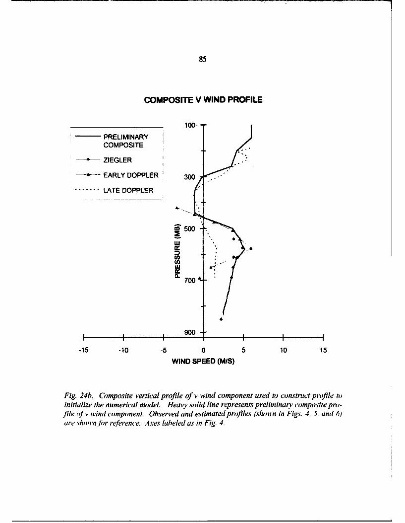
85

COMPOSITE V WIND PROFILE

100---PRELIMINARYCOMPOSITE

* ZIEGLER

- EARLY DOPPLER 300

....... LATE DOPPLER

o500 ,

.4a,,

U)

S700 ,

-15 -10 -5 0 5 10 15

WIND SPEED (M/S)

Fig. 24b. Composite vertical profile of v wind component used to construct profile toinitialize the numerical model. Heavy solid line represents preliminary composite pro-file oJfv wind component. Observed and estimated profiles (shown in Figs. 4. 5. and 6)are shown finr reference. Axes labeled as in Fig. 4.

86

the wind speeds were gradually increased from zero at 740 mb to the full preliminary

composite profile speed at 480 mb. Figure 25 shows the preliminary profile and the

final 3-D base-state profile.

The construction of the 2-D base-state profile required further manipulation to sat-

isfy the RAMS requirements for 2-D simulations. The version of RAMS employed

for this study allows 2-D simulations to be run only in an x-z slab. Thus only the u

component of the wind is allowed in such simulations. The 2-D profile was con-

structed from the 3-D base-state profile by using the magnitude of the total wind at

each pressure level as the -u component of the wind. The shape of the mountain and

its orientation with respect to the predominant wind flow permitted this approach.

The actual wind was predominantly southeasterly (particularly at low-levels) (Figs. 5,

6, and 25) and perpendicular to the mountain slopes. Similar wind vs. slope relation-

ships can be produced within the 2-D limitations by using the magnitude of the actual

wind as the -u component. The actual wind orientation is even less important in these

simulations since the magnitude was set to zero below the mountain top. Figure 26

shows the 2-D base-state wind profile.

5.3 Numerical Experiments

This section describes the five numerical simulation experiments conducted to test

the effect of differing initial conditions and forcing mechanisms on the simulated

storms. For each experiment, only one such condition or mechanism was varied from

the control's configuration. The simulation experiments will be referred to as EXPI

through EXP5 for the rest of this discussion. Table 3 provides a brief overview of all

the simulations conducted for this study. The term "standard" as used in the table re-

fers to the profiles or configuration used for the control simulation and described in

Chapter 4 and in Sections 5.1 and 5.2. Details of base-state profiles differing from

87

3-D BASE-STATE U WIND PROFILE

100

30- 3-D BASE-STATE

PRELIMINARYCOMPOSITE

50 "0

coC,Cm

w

700

900

-15 -10 -5 0 5 10 15

WIND SPEED (M/S)

Fig. 25a. Vertical profile of the u wind component of the "three-dimensional" hase-state profile (heay, solid line with ticks) used to build final profilefor input to the mod-el. The preliminary composite profile shown in Fig. 24a is showli. fr reference. Axesas labeled in Fig. 4.

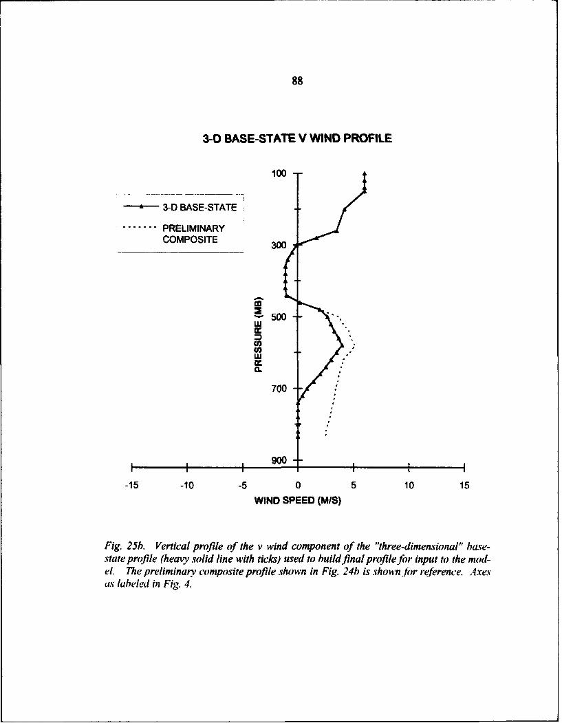
88

3-D BASE-STATE V WIND PROFILE

100

-J" 3-D BASE-STATE

....... PRELIMINARYCOMPOSITE 1 300

" 500w

700

-15 -10 -5 0 5 10 15

WIND SPEED (M/S)

Fig. 25b. Vertical profile of the v wind component of the "three-dimensional" base-state profile (heavy solid line with ticks) used to build final profile for input to the mod-el. The preliminary composite profile shown in Fig. 24b is shown.fhr reference. Axesas labeled in Fig. 4.

89

2-D MODEL WIND PROFILE

100

"COCA

m

1rn

I I I I I I

-15 -10 -5 0 5 10 15

WIND SPEED (M/S)

Fig. 26. Vertical wind profile used to initialize the numerical model. Wind speed inthis profile equals the magnitude of the total wind in the profiles shown in Fig. 25.Axes labeled as in Fig 4.

90

Table 3: Numerical simulation experimnt overview. "Standard" refers to conditionor process employed in the control simulation.

SIMULATION WIND PROFILE THERMODYNAMIC MICROPHYSICS SHORT-WAVENAME PROFILE RADIATION

CONTROL STANDARD STANDARD STANDARD STANDARD

EXPI CALM STANDARD STANDARD STANDARD

EXP2 50% SPEED STANDARD STANDARD STANDARDPROFILE

EXP3 STANDARD STANDARD STANDARD NONEEXP4 STANDARD STANDARD WARM RAIN STANDARD

MICROPHYSICS

EXP5 STANDARD MOISTENED STANDARD STANDARDI____ I_ _ LOWER LEVELS II_ I

those of the control simulation will be described as appropriate in the following chap-

ters.

EXPI and EXP2 evaluated the sensitivity of the simulated storms to the initial

base-state wind profiles. The intent behind this set of experiments was to isolate the

contribution of the environmental wind field to the development of the storms. EXPI

was initialized with calm winds throughout the depth of the atmosphere, while

EXP2's initial wind profile contained wind speeds half the magnitude of the control's.

EXP3 and EXP4 tested the sensitivity of the simulations to diabatic heating ef-

fects. The purpose of EXP3 was to evaluate the importance of solar heating in storm

development. EXP3's simulation was conducted with the RAMS short-wave radiation

package deactivated; in effect, "turning off the sun". It is important to note that deac-

tivation of the short-wave radiation package strongly impacts the behavior of the un-

derlying soil model. As in nature, removing the model's solar radiation also cuts off

91

surface heating and any thermal forcing resulting from such heating. The purpose of

EXP4 was to determine the importance of the ice-phase cloud microphysical processes

and their associated latent heating effects in storm development. EXP4 was con-

ducted with all the ice-phase microphysical processes deactivated and only the warm

rain microphysical parameterizations activated.

The final experiment, EXP5, was conducted to evaluate the effect on the simu-

lated storm of a moistened base-state moisture profile. The base-state moisture profile

was moistened by up to 0.5 g kg-1 below 720 mb. Section 9.1 describes the profile

used for EXP5.

Chapter 6

Analysis And Verification Of The Control Simulation

This chapter describes the results of the control simulation (referred to as the con-

trol). Section 6.1 provides a brief analysis of the simulated storm's evolution, and

Section 6.2 compares the simulated storm with the 31 July 1984 Doppler radar ob-

servations described in Chapter 3. Section 6.3 compares the microphysical evolution

of the simulated storm with the results of Lang's (1991) microphysical retrieval study

of a similar storm that occurred on 3 August 1984.

Throughout the simulation descriptions which follow in this and later chapters, the

following conventions will be employed. First, all time references will be simulation

times in seconds unless otherwise noted. Table 4 provides a conversion between

simulation times in seconds and hours and actual times with the 0945 MST model ini-

tialization time employed for these simulations.

All references wo heights will be based on the model's grid coordinates unless

otherwise noted. As discussed in Chapter 4, the model terrain elevations were ad-

justed so that the lowest terrain elevation in the model grid had a value of zero.

Thus, the model's lower boundary is located at approximately 1820 m MSL. All oth-

er model grid heights are reduced from actual MSL heights by this same amount. Ta-

ble 5 provides a conversion between model heights and actual MSL heights.

Finally, for the purposes of the following descriptions, a cell is defined as any

relative condensate and/or updraft maximum that exhibits vertical continuity. This

definition follows closely that used by Lang (1991) and employed in Chapter 3.

92

93

Table 4: Simulation time to actual time conversion chart.

SIMULATION SIMULATION ACTUAL TIME SIMULATION SiMULATION ACTUAL TMETWE (S) TIME (lit) (MT) TIME (M) TIME (MR1) (%w)

0 0.00 9:45 4680 1.30 11:03180 0.05 9:48 4860 1.35 11:06360 0.10 9:51 5040 1.40 11:09540 0.15 9:64 5220 1.45 11:12720 0.20 9:57 5400 1.50 11:15900 0.25 10:00 5580 1.55 11:181080 0.30 10:03 5760 1.60 11:211260 0.35 10:06 5940 1.66 11:241440 0.40 10:09 6120 1.70 11:271620 0.45 10:12 6300 1.75 11:301800 0.50 10:15 6480 1.80 11:331980 0.55 10:18 6660 1.85 11:362160 0.60 10:21 6840 1.90 11:392340 0.65 10:24 7020 1.95 11:422520 0.70 10:27 7200 2.00 11:452700 0.75 10:30 7380 2.05 11:482880 0.80 10:33 7560 2.10 11:513060 0.85 10:36 7740 2.15 11:543240 0.90 10:39 7920 2.20 11:573420 0.95 10:42 8100 2.25 12.003600 1.00 10:45 8280 2.30 12:033780 1.05 10:48 8460 2.35 12:06

3960 1.10 10:51 8640 2.40 12:094140 1.15 10:54 8820 2.45 12:12

4320 1.20 10:57 9000 2.50 12:154500 1.25 11:00

94

Table 5: Model height to actual height conversion.

MODEL HEIGHT ACTUAL HEIGHT(KM) (KM MSL)

0.00 1.820.25 2.070.75 2.571.25 3.071.75 3.572.25 4.072.75 4.573.25 5.073.75 5.574.25 6.074.75 6.575.25 7.075.75 7.576.25 8.076.75 8.577.25 9.077.75 9.578.25 10.078.75 10.579.25 11.079.75 11.5710.25 12.0710.75 12.5711.25 13.0711.75 13.5712.25 14.07

95

6.1 Analysis of Simulated Storm Evolution

Three primary cells developed during the control simulation. The origins of two

of the cells can be traced back to the earliest cloud and updraft development in the

simulation. The third cell developed primarily as a result of the upslope wind flow

induced by circulation of the first two cells.

The first condensate developed at 5760 s over the western slope of the mountain at

x = -2.5 km and z = 2.0 km. For the next 9 min, the cloud grew slightly and drifted

westward. By 6480 s the cloud had dissipated and was replaced by a new cloud

which formed at nearly the same position as the first. Figures 27 and 28 show analy-

ses of total condensate mixing ratio and vertical velocity, respectively, for 6480 s.

An analysis of the wind field for this time period showed that the first cloud drifted

away from the weak updraft which contributed to its initial development. The updraft

remained fixed at approximately its original position and led to the subsequent initia-

tion of the second cloud which quickly developed into a cell. During this same peri-

od, a low-level westerly flow of approximately 1.5 m s- developed below 2.0 km

west of the mountain ridge. Further investigation and the results of EXP3 (discussed

in Chapter 8) show that this westerly flow appeared to develop as a result of a dy-

namically induced mountain-wave circulation on the lee side of the mountain. The

interaction of this westerly flow with the easterly flow over the mountain created an

area of low-level convergence at approximately x = -2.5 km which supported the

fixed updraft described above. Figure 29 shows an example of this convergence.

By 6660 s the first cell (denoted hereafter as CCI) was located atx = -2.5 km and

z = 2.5 and was approximately 1.0 km deep. A new cell (denoted hereafter as CC2)

had developed just over the ridge at x = -1.0 km and z = 2.0 km. These cells

continued to develop slowly and drift slowly westward until 7200 s. During this peri-

96

CONTROL EXP

12. 0

-- -----------------------------------------------

-------------------------- --------10.-

. - - - - -

--- -

---------- -- ...

2.

I I II I I I I III 15.

-15.9 -19.0 -5.0 3.0 5.3. 10. 15..

X (KMI

TOTAL CONDENSATE WINDSIN VECTORS

Y = 0.00 KM T = 6480, S

Fig. 27. East-west vertical cross-section of simulated total condensate mitring ratiosoverlaid with simulated wind vectors for CONTROL simulation at 6480 s. Contoursare eveny 2.0 g kg' starting at 0.1 g kg1. Wind vector length shown in lower right-hand corner o1figure equals 50 m st. Vertical axis is labeled in kilometers above theminimum terrain elevation in the simulation grid (in this case 1.82 kin) as described inthe text. Horizontal axis is horizontal distance labeled in kilometers. The cross-sectionshown is located at y = 0.0 km and runs east-west, with the origin at Langmuir Labora-torv.

97

CONTROL EXP

12.,

10.-

8.-

4. .0--

4.0-

2. - ) ,

-15.0 -10.0 -5.0 0.0 5.0 19.0 15.9

X (KM)

VERTICAL WIND

Y = 0.00 KM T = 6480. S

Fig. 28. Eayt-west vertical cross-section of simulated vertical velocity contoured ever3.0 m v' starting at 1.5 m s' for CONTROL simulation at 6480s. Solid (dashed) con-tour sghow po•sitive (negative) vertical velocities. Axes labeled av in Fig. 27.

98

CONTROL EXP

12.-

--------------------------------------------------------------------------------------

--------------------------------------------------------------------------------------

............................................... ....................

. ....................-...-............. ........... --------------------------------------------------------------

2 ... ; . ... ............... . . . . . . . . . . . . . . . . . . . . . . .. 1. 50

4.

2. ................... .Q "... . .. . .. . -15

II II

-15.0 -10.0 -5.0 0.0 5.0 19.0 15.0

X (KM]

WESTERLY WIND

Y = 0.00 KM T = 6480. S

Fig. 29. East-west vertical cross-section of simulated u wind component contoured eV-

ety 3.0 m s-1 starting at 1.5 m s- for CONTROL simulation at 6480 s. Solid (dashed)contours show westerly (ea-rteriv) winds. Axes are labeled av in Fig. 27.

99

od, the convergent area remained at approximately x = -2.5 km. At the same time, a

shallow layer of easterly flow developed beneath the westerly flow, creating a second

low-level convergent area at x = -5.0 km (Fig. 30). The updraft associated with CC I

at 6660 s separated into two distinct updrafts after 6840 s. The upper portion of the

original updraft drifted westward with the condensate while the lower portion of the

updraft remained anchored at approximately x = -2.5 kin. CC2s original updraft

developed at about 6840 s and moved slightly westward before diminishing after 7200

s. At about this same time, the condensate associated with CC2 moved over the an-

chored updraft at x = -2.5 km. By 7200 s both major updrafts exceeded 4.5 m s-.

Figures 31 and 32 show analyses of total condensate mixing ratio and vertical veloc-

ity, respectively, for a time representative of this period--6840 s.

Between 7200 s and 7560 s, CC2's condensate drifted westward and merged with

the lower remnants of CCI's updraft. During this period, both cells' updrafts re-

mained separate and drifted westward. CC2's updraft increased to 6.7 m s', while

CCI's weakened to about 1.5 m s-1 by 7560 s. At 7200 s, a new updraft developed

west of CCl at x = -5.0 km in response to the secondary convergent area at that loca-

tion. This updraft began to strengthen as CCI moved into its vicinity. By 7560 s,

both CCI's original updraft and the new updraft were approximately the same

strength. A relatively strong easterly jet developed west of CCI at z = 3.75 km near

the level of the capping inversion. Several small cloud masses also formed over the

ridge between x = 0.0 km and x = 2.0 km and remained very weak with no asso-

ciated updrafts. The first significant development of rain water, pristine ice crystals,

and graupel occurred during this period. Prior to these developments, the condensate

consisted almost entirely of cloud water. Rain water first developed at 7100 s in CCI

near z = 3.75 kln. By 7380 s, most of the small area of rain had evaporated as it fell

100

CONTROL EXP

F ----------------------------------------------------------------------------------------

-----------------------------

n -------:- -

===.=:::;:-.-:o . , .- I* - ... ,

-5.0 0.0 5.0 1..0 15.0X (KM J

WESTERLY WIND

Y 0.00 KM T = 7200. S

Fig. 30. East-west vertical cross-section of simulated u wind component as in Fig. 249except.for CONTROL simulation at 7200 s.

101

CONTROL EXP

1--.--l -

-------........-- ----------------

2.0-o

e. - . . .- - -. -

0.-

-1.3 -10.0 -53335.3 10.0 15.0

X (KM)

TOTAL CONDENSATE WINDSIN VECTORS

Y = 0.00 KM T = 6840. S

Fig. 31. Analogous to Fig. 27, east-west vertical cross-section of simulated total con-densate mixing ratios overlaid with simulated wind vectorm for CONTROL simulation at6840 s. Contour label "1"represents 0.1 g kg1.

102

CONTROL EXP

12. "i

_r

-- 16. -5.3 6.0 5.0 10.0 15.6

X (KM)

VERTICAL WIND

Y = 0.00 KM T = 6840. S

Fig. 32. Analogous to Fig. 28, east-west vertical cross-section of simulated vertical ve-locity for CONTROL simulation at 6840 s.

103

out of CCI, and CCI drifted away. Both pristine ice crystals and graupel developed

in CCl near z = 4.0 km between 7110 and 7290 s. Rain water developed at 7560 s

near the center of CC2 between z = 3.25 and 3.75 km. Figures 33 and 34 show

analyses of total condensate mixing ratio and vertical velocity, respectively, for

7560 s.

By 7740 s, CC2 had become the dominant cell in the merged storm with maxi-

mum total condensate mixing ratios of 3.4 g kg'. A new cell (denoted hereafter as

CC3) developed at x = 0.0 km and z = 1.75 km with a weak updraft. CC3's devel-

opment appears to have resulted primarily from upslope flow induced by the inflow

into CCI and CC2. CCI's original updraft dissipated by this time and was replaced

by the newer updraft at x = -5.0 km which had strengthened to 4.5 m s-1. The sec-

ondary area of low-level convergence continued to support CCI's new updraft and

also provided support to CC2's updraft. Graupel first developed in CC2 at this time

between z = 3.0 and 4.5 km. Ice crystals continued in CCl and also began to devel-

op in CC2 at this time.

At 7920 s the first precipitation developed as a rain shaft from CC2 between x =

-3.0 and -4.0 km. At this time also, CCI had regenerated significantly while CC2

weakened slightly. Maximum total condensate mixing ratios in both CCI and CC2

ranged from 2.0 to 3.0 g kg-'. The rapid regeneration of CCI can be attributed to the

rapid strengthening of its new updraft to over 10.0 m s-1. At the same time, another

new updraft also developed just to the west of CCI in response to the low-level con-

vergence which continued near x = -6.0 km. Graupel and rain water redeveloped in

CC1 between z = 2.25 and 3.75 km. CCI's total condensate maximum consisted en-

tirely of cloud water, while CC2's maximum consisted of a mixture of ice crystals,

104

CONTROL EXP

12. ,.

-----------------------------

8. .". .

~ 6.

-15.3 -1. --. -. 5- -3. - -

X (KM)TOTAL CONDENSATEWIO

IN VECTORSY 0.00 KM T 7560. S .

Fig. 33. As in Fig. 27, east-west vertical cross-section of simulated total condensatemixing ratios overlaid with simulated wind vectors for CONTROL simulation at 7560 s.Contour label "1" represents 0.1 g kg

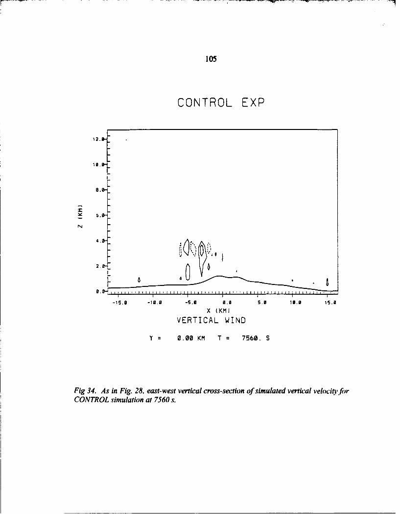
105

CONTROL EXP

2.-2H

-15.9 -10.0 -5.91 0.91 5.9 19.0 15.11

X (KMJVERTICAL WIND

Y = 0.00 KM T = 7560. S

Fig 34. As in Fig. 28, east-west vertical cross-section of simulated vertical velocity firCONTROL simulation at 7560 s.

106

cloud water, and graupel. Figures 35 and 36 show analyses of total condensate mix-

ing ratio and vertical velocity, respectively, for 7920 s.

CCI had become the dominant cell at 8100 s with a maximum total condensate

mixing ratio exceeding 4.0 g kg-". By this time both updrafts in the vicinity of CCI

had merged to produce a double maxima updraft. The upper portion of the updraft

had strengthened to 13.0 m st' while the lower portion exceeded 4.5 m s1. Both por-

tions of the updraft continued to be supported by the low-level convergence near x =

-6.0 km. CC2's updraft remained distinct with a maximum strength of over 4.5

m s1. A significant downdraft of 5.5 m s- developed at this time between the up-

drafts associated with CCI and CC2 and at a height of z = 3.75 km. CC3 remained

very weak with several weak updrafts in its vicinity. A new area of rain water devel-

oped near CCI's maximum total condensate atz = 4.25 km. CCI's total condensate

maximum at this time consisted of a mixture of ice crystals, cloud water, rain water,

and graupel. Figures 37 and 38 show analyses of total condensate mixing ratio and

vertical velocity, respectively, for 8100 s.

By 8280 s, CCl was clearly the dominant cell with double maxima in both the

total condensate mixing ratio and the vertical velocity fields. Maximum total conden-

sate mixing ratios exceeded 4.0 g k41 in the upper portion of the cell and 2.0 g kg-'

in the lower portion. The cell's condensate reached a maximum height of about 6.0

kmn. The upper portion of the updraft remained strong at 11.0 m s- while the lower

portion strengthened to over 7.5 m s-1. The low-level convergence continued beneath

CCI's updraft while a divergent flow developed at z = 5.25 km near the top of the

updraft. As rain began to fall from CCI, the storm's rain shaft increased in size to

approximately 2.5 km wide. CC2 remained evident in the total condensate analysis as

a turret of condensate on the eastern side of the storm. CC2's updraft diminished

107

CONTROL EXP

-- -----------------------------------------------

- ------------------------------------- --

-- - - - -- -- -- ---- - - - .- .-- ---- -. . . .- -

e.°

[ ....................................r

4.0-

4.. .. .

2.0-

0.

-15.6 -19.9 -5.3 3.3 S.0 13.3 1S.0

X (KM)

TOTAL CONDENSATE WINDSIN VECTORS

Y = 0.00 KM T z 7920. S

Fig. 35. East-west vertical cross-section of simulated total condensate mixing ratiosoverlaid with simulated wind vectors, av in Fig. 27, except for CONTROL simulation at7920 s. Contour label "1" represents 0.1 g kgt.

108

CONTROL EXP

N4.

4. 0-

I I 1 1 1 1 i f1 1 # 1 1 H I l 1 - f I . 1 1 [ . . . .

04. 5.0 10.0 15.3

X (KM)

VERTICAL WIND

Y = 0.00 KM T = 7920. S

Fig. 36. East-west vertical cross-section of simulated vertical velocity, as in Fig. 28,except for CONTROL simulation at 7920 s.

109

CONTROL EXP

------------ -------------------

-------------------------------

r - -- - - - - - -

S.. ........... .............

Fo0o6.- ...J .........

4 15.i0 -0 .• 5.. 6 15.

X (KM)

TOTAL CONDENSATE WINDS

IN VECTORS

Y = 0.00 KM T = 8100. S

Fig. 37. Analogous to Fig. 27, east-west vertical cross-section of simulated total con-densate mixing ratios overlaid with simulated wind vectors for CONTROL simulation at8100 s. Contour label "1" represents 0.1 g kg'.

110

CONTROL EXP

12. ý

IS.0

-15.0 -10.9 53 . 10.0 15.0

X (KM)

VERTICAL WINO

Y = 0.00 KM T =- 8100. S

Fig. 38. Analogous to Fig. 28, east-west vertical cross-section of simulated vertical ve-locitv for CONTROL simulation at 8100 s.

111

considerably in size from the previous analysis. CC3 had increased in size (primarily

by building westward), but still contained no significant updrafts. Aggregated snow

flakes first developed at this time in CC2. Both CCI and CC2 contained well-defined

graupel shafts. CC3's condensate at this time consisted entirely of cloud water.

CC2's area of maximum total condensate consisted primarily of pristine ice crystals

but also contained a mixture of graupel, cloud water, and aggregated snow flakes.

CCI's maxima on the other hand, consisted primarily of cloud water, with smaller

amounts of rain water, graupel, and pristine ice crystals.

At 8460 s, CC1 continued to strengthen with maximum total condensate mixing

ratios exceeding 6.0 g kg-' at approximately 6.0 km near the top of the cell. CCl's

updraft again contained a double maxima with vertical velocities exceeding 10.5 m s-'

and 14.5 m s-1 in the upper and lower maxima, respectively. By this time, the area of

low-level convergence supporting CCl's updraft had moved slightly westward to x =

-7.5 km. This movement resulted from the westward expansion of the cool easterly

outflow associated with the precipitation shaft. Meanwhile the divergent flow contin-

ued near the top of CCl's updraft at z = 5.75 km. CCI's condensate reached a

maximum height of about 7.5 km at this time. CC2 remained distinct as a turret of

condensate on the eastern edge of the storm, however, its updraft had weakened to

about 1.5 m s-. At the same time, CC3 had strengthened significantly and moved

slightly westward. CC3's maximum total condensate mixing ratios had increased to

2.0 g kg', and its updraft developed to a maximum of 4.5 m s-'. Both CCI and CC2

were dominated by the ice phase at this time. The areas of highest total condensate

mixing ratios in both cells consisted primarily of ice crystals, while very little cloud

water existed anywhere in the cells. Aggregated snow flakes had also developec by

this time in CC1. As expected from the location of the pristine ice crystals, the ag-

112

gregates were located near the total condensate maxima in both cells. Graupel also

continued in both CCI and CC2. Rain water developed for the first time in CC3.

CCI continued to dominate the simulation at 8640 s. While CCl's maximum to-

tal condensate mixing ratios decreased slightly to 5.9 g kg-', its updraft continued to

exhibit a double maxima with vertical velocities remaining about the same strength as

at 8460 s. The low-level convergence at the outflow boundary continued to support

CC 's updraft at this time, while the divergence near the top of the updraft continued

to increase in height to approximately 6.5 km. The downdraft located just to the east

of CCI's updraft strengthened again to 4.5 m s-1. CCI's condensate reached a maxi-

mum height of approximately 9.0 km. A new updraft with maximum vertical veloci-

ties of 4.5 m s-1 developed at this time between the condensate masses associated with

CCI and the remnants of CC2. CC3 continued to strengthen and move slowly west-

ward to about x = -1.0 km. While CC3's total condensate mixing ratios remained

virtually unchanged from 8460 s, its updraft increased to a maximum of 7.5 m s-1. A

very weak westerly flow, resulting from the precipitation-induced outflow, developed

at this time near x = -4.5 km and z = 1.5 km. The interaction of this westerly flow

with the prevailing easterly flow at that location produced another area of conver-

gence which helped strengthen CC3's updraft. The ice phase continued to dominate

CCI at this time. The bulk of CCI's condensate, particularly near its maximum, con-

sisted of pristine ice crystals. At the same time, a deep shaft of graupel had devel-

oped near the center if the cell. The areas of aggregates continued near the ice

crystal maxima in both CCI and CC2. The bulk of CC3's condensate remained cloud

water with smaller amounts of graupel and rain water. Figure 39 shows analyses of

total condensate, cloud water, rain water, pristine ice crystals, graupel, and aggre-

113

CONTROL EXP

12.0-

- ------------------------------------------------

------------------------

- ---------------------------------------

8.0-4.0-2.0--

-.0-

-15.0 -10.0 -5.0 0.0 5.0 10.0 15.2

X (KM)

TOTAL CONDENSATE WINOSIN VECTORS

Y = 000 KM T= 8640. S

Fig. 39a. East-west vertical cross-section of simulated total condensate mixing ratiosoverlaid with simulated wind vectors, as in Fig. 27, except for CONTROL simulation at8640 s. Contour label "1" represents 0. 1 g kgt'.

114

CONTROL EXP

12.0-

10.1-

8.3"

2. @-c

-15.0 -10.0 -5.0 0.0O 5.0 10•.@ 15.2

X (KM)

CLOUD WATER

Y 0.00 KM T = 8640. S

Fig. 39h. East-west vertical cross-section of simulated cloud water mixing ratios con-toured every 2.0 g kg-' starting at 0. 1 g kg-' for CONTROL simulation at 8640 s. Axeslabeled as in Fig. 27. Contour label "I" represents o. I g kg-'.

115

CONTROL EXP

12.

a..-

N

-15.9 -19.9 -5.9J 9.9 5.9 19.9 15.9]

X (KM)

RAIN

Y = 0.00 KM T 8640. S

Fig. 39c. Analogous to Fig. 39b, east-west vertical cross-section of simulated rain wa-ter mixing ratios for CONTROL simulation at 8640 s. Contour label "I" represents 0. 1g kg'.

116

CONTROL EXP

12.-

8. Oý._

E-6.4

2. 1

-15.9 -1.9 -5.90 0.9 5.0 19.9 15.9

X (KM)

PRISTINE ICE

Y = 0.00 KM T = 8640. S

Fig. 39d. Analogous to Fig. 39b, east-west vertical cross-section of simulated pristineice crystal mixing ratios for CONTROL simulation at 8640 s. Contour label "1" repre-sents 0. 1 g kg-'.

117

CONTROL EXP

12.0-

-15.8 -10.0 -5.9 9.9 5.0 10.0 15.9

X (KM)

GRAUPEL

Y = 0.00 KM T = 8640. S

Fig. 39e. Analogous to Fig. 39b, east-west vertical cross-section of simulated graupelmixing ratios for CONTROL simulation at 8640 s. Contour label "1" represents 0. 1g kg-'.

118

CONTROL EXP

iS. 0-

4. 04

r

-15.0 -10.0 -5.9 0.0 5.0 10.0 15.0

X (KM)

AGGREGATES

Y 0.00 KM T = 8640. S

Fig. 39f Analogous to Fig. 39b, east-west vertical cross-section of simulated aggre-gated snowflake mixing ratios for CONTROL simulation at 8640 s. Contour label "I"'represents 0. 1 g kg'1.

119

gated snow flake mixing ratios, respectively, for 8640 s. Figure 40 shows an analysis

of vertical velocity for 8640 s.

By 8820 s CC2 had lost its identity as CC3 moved westward and CC3's conden-

sate merged with CCL. The maximum total condensate mixing ratio exceeded 5.9

g kg-' in both CCI and CC3, with the highest mixing ratios located above 4.0 km in

both cells. CCI's condensate reached a maximum height of 10.25 km, and precipita-

tion first developed from CC3 at this time. CCI's updraft contained several local

vertical velocity maxima with the primary maximum of 16.6 m s-1 located at 8.0 km

near the top of the cell. The precipitation-induced outflow below CCI continued to

create areas of convergence both to the west and east of the main precipitation shaft.

The westerly flow portion of the outflow first noted at 8640 s, became better defined

by this time. The divergent flow near CCI's updraft extended to nearly z = 8.0 km.

The downdraft on the eastern edge of CCI weakened considerably, while a new

downdraft of about 6.2 m s-1 formed near the center of the precipitation shaft. CC3's

updraft continued at its previous strength of 7.5 m s-1, but the updraft's structure be-

came much less organized. A weak divergent flow developed at 4.75 km near the top

of CC3's updraft. The new updraft which had developed between CCI and CC2 at

8640 s weakened dramatically to 1.5 m s-1 as it came under the influence of the down-

drafts from CC1 and CC3 as they merged. By this time, the bulk of CC! 's conden-

sate consisted of either pristine ice crystals or aggregated snow flakes. Aggregate

mixing ratios exceeded 2.0 g kg-'. The graupel shaft continued in CCI, and graupel

reached the surface for the first time. CC3's condensate still consisted primarily of

cloud water, but pristine ice crystals had developed for the first time. The area of

graupel expanded, and rain reached the surface for the first time out of CC3. Figures

120

CONTROL EXP

12.4

B.Z.- /-8114

N.• .I. . . I ,I . .. I' I

A

-15.1 -16.3 -5.6 6.3 5.6 '6.6 15.6

X (KM)

VERTICAL WIND

Y - 0.00 K(M T = 8640. S

Fig. 40. East-west vertical cross-section of simulated vertical velocity as in Fig. 28.except for CONTROL simulation at 8640 s.

121

41 and 42 show analyses of total condensate mixing ratio and vertical velocity, re-

spectively, for 8820 s.

At 9000 s, CCl still dominated the merged storm. The maximum total condensate

mixing ratio exceeded 6.0 g kg-' in CCI, while barely reaching 2.0 g kg-' in CC3.

CC I's condensate reached a maximum height of 11.0 km. The updraft structure be-

came very complicated as CCI and CC3 began to interact with each other. CCI's

main updraft contained a maximum vertical velocity of over 10.5 m s-. Meanwhile a

secondary updraft core had developed slightly to the east of the original. This core

contained a maximum vertical velocity of 7.5 m s'. At the same time, CC3's updraft

had become more organized and strengthened to 10.5 m s-. By this time the low-

level outflow convergence areas were very well defined. The convergent flow on the

western side of the outflow spawned the development of several updrafts on the west-

ern edge of CCI, while the strong low-level convergence on the eastern side of the

outflow supported the strengthening of CC3's updraft. The upper-level divergence

near CCI's updraft continued, but became less organized than at previous times. The

same basic microphysical structure existed in the cells at this time as reported for the

previous time.

6.2 Comparison With Radar Observations

This section presents a comparison of the control simulation results with the Dop-

pler radar storm observations from the 31 July 1984 case. The two-dimensional na-

ture of the numerical simulations conducted for this study naturally limit direct

comparisons with storm observations, however, qualitative and some quantitative

comparisons can yield a realistic assessment of the simulation's accuracy. Establish-

ing the fidelity of the control simulation represents a crucial first step of this study

122

CONTROL EXP

12.o,

-------------------------------

-------------------------

1 9. _

--4. - -" - - - .-

-0--0

-.o -19.9 -5.9 9.9 5.9 19.9 5.

X (KM)

TOTAL CONDENSATE WINDSIN VECTORS

Y = 0.00 KM T = 8820. S

Fig. 41. East-west vertical cross-section of simulated total condensate mixing ratiosoverlaid with simulated wind vectors, as in Fig. 27, cept for CONTROL simulation at8820 s. Contour label "1" represents 0. 1 g kg'.

123

CONTROL EXP

12.0

10.8.-1

v 6.0-

N "Q

X (KM)

VERTICAL WINO

Y 0.00 KM T = 8820. S

Fig. 42. East-west vertical cross-section of simulated vertical velocitY, as in Fig. 27.exceptYfor CONTROL simulation at 8820 s.

124

since the numerical simulation experiments discussed in later chapters will be com-

pared to the control.

Given the limitations imposed by the two-dimensionality of the numerical simu-

lation, the simulation compared very favorably with the Doppler radar observations

collected on 31 July 1984. The simulation captured most of the important cell and

storm features and characteristics noted in the description of the radar observations in

Chapter 3.

6.2.1 General Comparisons

The control simulation captured the multicellular nature of the storms as observed

by the radars. Three dominant cells developed in the simulation while seven cells

were observed by the radars. Some of this difference can be attributed to the two-

dimensional nature of the simulation which naturally decreases the amount of space

available for cell development. Second, as described later, the convective develop-

ment in the simulation lags the observations by between 15 and 40 min. The final

four observed cells developed in the last 18 min of the analysis. It is likely that the

simulation lag resulted in the simulation ending before further cell development oc-

curred.

The development of low-level convergence areas in the simulation compares rea-

sonably well with that seen in the observations. Since the simulation was conducted

in two dimensions, it could not capture the terrain-induced channelling convergence

found in the observations. The simulation did show the development of low-level

convergence areas in response to the mountain-valley flow as observed in the synthe-

sized wind fields. In both the simulation and in the observations, the low-level con-

vergence areas were crucial to convective initiation. These convergence areas

primarily determined the location of initiation. The simulation also reasonably repro-

125

duced the development of upper-level divergence areas above the strongest cells. For

the most part, the simulation's upper-level divergence areas were weaker than those in

the synthesized wind fields.

In both the observations and in the simulation, the convective initiation occurred

over or very near the ridges. The simulated initiation locations tended to be slightly

to the west of the ridge lines while in the observations, the initiation locations

generally were either directly over or slightly to the east of the ridge lines. The mag-

nitude of the distance differences between observed and simulation initiation locations

was always less than 5.0 km. The two-dimensional nature of the simulation again ex-

plains in part the difference in the pattern of initiation locations. As described in

Chapter 3, the initiation locations were strongly influenced by the channelling conver-

gence induced by the narrow valleys. These features could not be adequately repre-

sented in a two-dimensional simulation. As a result, the simulation's initiation

locations are more strongly determined by the thermally-driven mountain-valley

flows.

As mentioned previously, the simulation's convective development lagged that ob-

served by the radars by a significant amount of time. The two-dimensional nature of

the simulation makes it difficult to determine the exact timing difference: As ex-

pected, investigation of individual features yields different timing differences. For

example, a comparison of the simulated maximum updrafts and downdrafts with those

synthesized from the radar observations (Fig. 43) shows good agreement between the

simulation and the observations with a simulation lag time of about 14 min. The

simulation's condensate first developed at 1115 (simulation time) and the condensate

first extended down to 1.5 km (3.3 km MSL) at 1151 (simulation time). Comparing

this time with the observed radar reflectivities of 30 dBZ at 3.3 km MSL at 1116

126

SYNTHESIZED AND SIMULATED VERTICAL VELOCITIES

OBSERVATION TIME (MST)

--10

I- I

V- O - T--

I- -. - ----.

>~ -5ji ?

-10 /4

-15 1 1 1 i i 1 1 I L I I I I I L .I 1 -1 1 1 1 I a I

SIMULATION TIME (SEC)

Fig. 43. Time evolution of synthesized (heavy curves with ticks) and CONTROL simu-lation simulated (light curves without ticks) maximum and minimum vertical velocities.Solid curves show maximum upward vertical velocities (positive w). Dashed curv.esShow maximum downward vertical velocities (negative w). Vertical axis is vertical ve-locitv in m s-1, bottom horizontal axis is simulation time in seconds, and top horizontalaxis is observation time in hours and minutes (MST).

127

MST yields a lag time of at least 35 min. It is important, therefore, to exercise cau-

tion when attempting to make one-to-one temporal comparisons between the simulated

storms and the observed storms.

The simulated updrafts qualitatively compared quite well with those analyzed from

synthesized wind fields. The updrafts in both cases agreed quite well in both horizon-

tal and vertical extent. The width of the simulated updrafts averaged only slightly less

than the 2.0 km widths seen in the observations. The simulated updrafts were about

8.0 km deep compared to the 7.0 to 8.0 km depth of the observed updrafts. The

comparison of the maximum updrafts (again using Figure 43) shows that, taking into

consideration the timing lag discussed above, the maximum strength of the simulated

updrafts agrees very well with the observed maximum updrafts. In general, the de-

velopment of the simulated updrafts also follows quite well that seen in the synthe-

sized wind fields. In both cases cells frequently contained single updrafts with

vertical velocities of 12.0 m s-1 or less. Also in both cases, early in the convective

development, the updrafts are strongest in the low- to mid-levels, and both show a

tendency for the updraft maxima to move to the mid- to upper-levels as the cells ma-

ture. The simulation showed that some cells developed either multiple updrafts or

updrafts with two or more local maxima in the vertical direction. The observed

storms also showed a similar phenomenon. The simulated updrafts for the most part

are nearly vertical with very little tilt. This contrasts markedly with the observed up-

drafts which frequently tilted backward (away from the inflow). As observed in the

synthesized wind fields, the simulated updrafts developed most often near regions of

low-level convergence. The stronger updrafts were associated also with regions of at

least weak upper-level divergence.

128

The simulated downdrafts do not compare nearly as well with observations. A

comparison of the horizontal and vertical extent of the simulated downdrafts with the

observed shows only a poor correspondence. The simulated downdrafts for the most

part are much narrower and shallower than those observed. A comparison of the

maximum downdrafts (again using Figure 43) shows agreement between both the

simulation and the observations after taking into consideration the simulation's timing

lag. The simulation fails to develop the strong downdrafts of over 9.0 m s-' seen in

the observations between 1158 and 1201 MST. The simulation also fails to capture

the broad areas of strong downdrafts as observed. Instead the simulated downdrafts

were usually confined to very narrow regions. The simulated downdrafts were lo-

cated primarily in low-levels as was predominantly the case with the observations.

However, the simulated downdrafts could also be found throughout nearly the entire

vertical extent of the model domain.

The analysis of the validity of the simulation's precipitation development is some-

what hindered by the fact that the lowest radar analyses were performed at 3.3 km

MSL. Thus it is not possible to determine precisely where or when the precipitation

was associated with radar returns at that level. If it is assumed that the precipitation

shaft is approximately the size of the radar maximum at the 3.3 km MSL analysis lev-

el, then the simulation's precipitation shafts compared very favorably with those ob-

served. In both cases, the precipitation shafts early in the precipitating stage ranged

from 1.0 to 1.5 km in diameter and increased to 2.5 to 3.0 km in the latter part of the

mature stage. Also in both cases, several precipitation shafts developed. The ob-

servations contained more precipitation shafts, and they were farther apart than in the

simulation; a discrepancy most likely resulting from the limitations imposed by the

two-dimensional nature of the simulation. In both the simulation and in the observa-

129

tions, the precipitation shafts were located near or directly beneath major updrafts.

The separation between precipitation and updrafts was generally greater in the ob-

servations than in the simulation.

The simulation's ability to capture the vertical development of cells can be as-

sessed by comparing the height of simulated condensate with the height of radar re-

turns. A comparison of the maximum heights of the simulated condensate with the

maximum height of radar returns (Fig. 44) shows a lag of approximately 23 min be-

tween the simulated development and the actual development similar to that discussed

earlier in this section. Taking this lag into consideration, the simulation captured the

rapid increase in maximum radar return height observed between 1146 MST and 1152

MST. Through most of the simulation, the maximum condensate heights remained

2.0 to 3.0 km lower than the observed radar return heights. The simulation indicated

a slow steady growth in height to about 5.25 km (7.0 km MSL) followed by a single

rapid surge in height to near the absolute maximum seen in the radar data. The rapid

development which followed the penetration of the 5.25 km (7.0 km MSL) level ap-

pears to result from the favorable moisture and temperature profiles above that level.

The relatively strong inversion and the very dry layer which exk',ted below 5.25 km

(7.0 km MSL) capped the convective development until late in the simulation. A

similar capping phenomenon can be seen in the observed early convective develop-

ment where no echoes penetrated above 6.5 km MSL until after 1I 3 MST. The

simulation failed to capture the observed double peak in maximum heights seen in

Figure 44.

The lifetime of the simulated cells compared very closely with those observed in

the radar observations. The longest-lived simulated cell, CCI, existed for 42 min

prior to the simulation's termination. This cell likely would have existed for up to

130

OBSERVED AND SIMULATED CLOUD TOP HEIGHTS

OBSERVATION TIME (MST)

1- 1 ~ , ' ' -Y % CYJ CJ

16 , , , , , , , , , , , , , , , , , , , 14

14 12

-12 -10

- Cn

C,,

•10 8

000 X"8 6 5

<6 4,-

4 2

21 0

SIMULATION TIME (SEC)

Fig. 44. Time-height cross section showing maximum simulated total condensateheight for the CONTROL simulation (plain curve) and maximum height of observed re-flectivitv (solid curve wfth ticks). Plain curve shows maximum height of 0. 1 g kg' totalcondensate mixing ratios. Ticked curve shows maximum height of 10 dBZ radar re/lec-tivities. Right vertical axis is labeled in kilometers above the minimum terrain elevationin the simulation grid (in this case 1.82 /om) as described in the text, and left verticalaxis is height relative to mean sea level in kin. Bottom horizontal axis is simulationtime in seconds and top horizontal axis is observation time in hours and minutes MST

131

another 10 min had the simulation been extended. CC2 existed for 36 min before be-

ing absorbed in CCl. Finally, CC3 existed only 21 min before the simulation ended.

This cell was in the early stages of development and likely would have developed for

some time had the simulation been extended. These lifetimes compare well with the

20 to 60 min lifetimes seen in the observations. It is likely that had the simulation

been extended, the storm would have grown and eventually decayed with the result

that the overall storm lifetime also would have compared favorably with the 1.0 to 1.5

hr storm lifetime observed by the radars.

Only one of the simulated cells, CC1, showed the tendency for periodic reintensi-

fication seen in the observed cells. In the simulated cell, the cycle of reintensification

occurred early in the cell's development between 7200 and 7740 s simulation time.

The simulated cell's reintensification period of 9 min agreed well with the observed

reintensification periods of 6 to 12 min.

Finally, the simulation captured reasonably well the intercellular relationships seen

in the radar data and the synthesized wind fields. The simulation accurately repro-

duced the alternating intensification between cells described in Chapter 3. CC2 ini-

tially developed as the strongest cell in the simulation. Then by 8100 s, CCI had

become the dominant cell. Later, as CCI began to mature and weaken, CC3 began to

intensify. Additionally, the simulation reproduced the observed tendency for intensi-

fying cells to entirely absorb the condensate and circulation of surrounding cells. For

example, CC2 was absorbed into CCM as CC1 and CC3 merged. The simulation to a

lesser extent captured the strong observed relationships between the circulations of

neighboring cells. Only in a few cases did the divergent outflow at the top of a cell

influence or feed the inflow of a neighboring cell. The best example of this occurred

between CC3 and CC1 late in the simulation.

132

6.2.2 Detailed Comparisons

Comparisons of simulation results at selected times throughout the storm develop-

ment with radar observations and synthesized wind fields provide more detailed in-

sight into the accuracy of the simulation. The comparisons were made using the

vertical cross sections of the observed storm cell referred to as C2 in Chapter 3. This

cell was chosen because of its proximity to the location of the simulation domain.

The comparison times were chosen to account for the simulation's apparent lag time

from the observed time as discussed in the previous section. The most rapid cell de-

velopment occurred in the simulation immediately after penetration of the capping in-

version. Unfortunately, the corresponding penetration in nature occurred during the

radar data gap between 1119 and 1134 MST. As a result, no comparisons between

the simulation and observations could be made for this crucial period in the storm's

development.

The first comparison was made using the simulation results at 6840 s (Figs. 31

and 32) and the ob -rvations from 1119 MST (Fig. 8). This comparison examines the

very early stages of cell development. Both the simulation and the observations show

only very weak development occurring at this time. No vertical cross-sections were

made from the observations at this time, however, the horizontal cross-sections show

only very weak echoes existed above 5.3 km MSL in the vicinity of C2. The simu-

lated cells extended to only 3.75 km (4.5 km MSL). The observed echo and the

simulated cell were both approximately 1.5 km wide. The observations at 1119 MST

did not support the synthesis of vertical velocities in the vicinity of the echo. The

simulated vertical velocities were only 1.5 m s-1.

The next comparison was made using simulation time 8460 s and observations

from 1134 MST. This comparison examines the early part of the cell's mature stage.

133

Figure 45 shows the simulated total condensate and wind fields for 8460 s, and Fig-

ure 46 shows the radar reflectivity and synthesized wind fields for 1134 MST. The

two figures show many similar features present in both the simulation and in the ob-

servations. In both cases, the cell extends to approximately the same MSL height.

Both cells contain a relatively strong core of high reflectivity (observed) or total con-

densate mixing ratio (simulated) located just to the west of the cell's main updraft.

Both cases also show low- to mid-level inflow into the eastern side of the cell with

relatively strong mid- to upper-level outflow on the western side. Additionally, both

cases exhibit a developing weak westerly inflow into the cell at very low levels.

The comparison also shows several marked differences between the simulation and

the observations. First, the simulated cell developed several kilometers west of the

observed cell. The cause of this difference is not clear, but may be attributed to the

lack of three-dimensional forcing effects in the simulation or perhaps an unrealistical-

ly strong initial wind profile. Second, the simulation contains a significant total con-

densate maximum near the top of the cell which does not appear as a maximum in the

observed reflectivity field. Further inspection shows the simulated maximum con-

sisted primarily of pristine ice crystals. The lack of a similar upper-level maximum in

the observed reflectivity analysis may be attributed to the low radar reflectivity of

such ice crystals (Battan, 1973). This phenomena was noted in almost all of the simu-

lations conducted for this study. Third, the simulated cell's updraft was significantly

stronger than that observed in C2 (14.6 m s-' vs. 9.0 m s-'). Fourth, the simulated

cell measured only about 3.5 km across, while the observed cell measured nearly 7.0

km across.

The final comparison was made using simulation time 9000 s and observations

from 1152 MST. This comparison examines the latter part of the cell's mature stage.

134

CONTROL EXP

12.0-

- ----------------- - - - - - - - -

- - - - - - - - o- - - - - - -b. 0

-------- T---

-15.3 -13.3 --5.3 3.3 5.3 13.3 15.3

X (KMI

TOTAL CONDENSATE WINDSIN VECTORS

Y = 0.00 KM T = 8460. S

Fig. 45. Analogous to Fig. 27, east-west vertical cross-section of simulated total con-densate mixing ratios overlaid with simulated wind vectors for CONTROL simulation atX460 s. Contour label "1" represents 0. 1 g kg'.

135

07/31/841 134 MSTCROSS-OECT IONS 4 RAOAR4.26KM 'PEFLECTIVITTY WOZ)

•• 10 10

100

-I -15)

Sis

-1!10

Fig. 46a. Horizontal cross-section of observed radar reflectivities as in Fig. IOa, ex-cept at 1134 MST and 4.3 nU MSL. Line AB shows location of vertical cross-section inFig. 46b. Line CD was not used.

136

R C1.S.-L.S) AT 0.0 OEG 1134 MST07/31/841STORM MOTION COMPONENT IN PLANE - 20.0 MI/lq i I I I i I I I" I I l I I I .. I I I i

12-

Z 10

-- 10 t

S10 "* -10

10-1

i s 2 0 I S \ % pP • ", ql . i o 4 0 : 15, '.

x -. -6.0 -1.0 -2.0 0.0 2.0 '.0 6.o 6.0 20.0T -1.5 -1.5 -1.5 -3.5 -1.5 -!.5 -1.5 -1.5 -I.5

VELOC ITT/REFLECTIVITY

Fig. 46b. As in Fig. lOh, vertical cross-section of observed radar reflectivities and vec-tor velocities at 1134 MST. Cross-section location AB is shown in Fig. 46a.

137

Figure 47 shows the simulated total condensate and wind fields for 9000 s, and Fig-

ure 48 shows the radar reflectivity and synthesized wind fields for 1152 MST. It is

important to note that in the previous two comparisons, the single simulated cell

(denoted CCI in earlier discussions) was compared with the observed cell C2, while

in this comparison, CCI corresponds more closely to the observed cell Cl. While

this change is significant, the qualitative nature of these comparisons still allows an

assessment of the simulation's accuracy. The two figures again show many similar

features between the simulation and the observations. In both cases, two cells exist in

nearly the same configuration. The western cell in both cases extends to nearly the

same MSL height. Both western cells contain strong downdrafts associated with the

cells' precipitation shafts. In both cases, low-level flow enters the eastern side of the

eastern cell, rises through the eastern cell's updraft, exits the western side of the east-

ern cell, then enters the western cell's updraft to finally exit in the western cell's out-

flow region. The horizontal dimensions of both simulated cells compared very

favorably with those observed. Also in both cases, there are two precipitation shafts

with an area between the shaft which contained little or no precipitation.

In addition to the change in cell correspondence described in the previous para-

graph, this comparison showed several other major differences between the simulation

and the observations. Several of the differences noted in the previous comparison

were also noted in this comparison. First, the simulated cells were again located sev-

eral kilometers west of the observed locations. Second, the western simulated cell

again contained a tG,,, condensate maximum near the top of the storm with no cvrr.-

sponding reflectivity maximum in the observations. Third, the maximum simulated

vertical velocity exceeded that observed in CCI by over 4.0 m s-1 . Finally, the simu-

138

CONTROL EXP

12. 0-

--- ---- - - -- -- -- -- -- -- -- -- -- --

---- ----------------------

410.

2.0-

-15.0 -10.0 -5.0 :.0 5.0 10.0 15.0

X (KM)

TOTAL CONDENSATE WINDSIN VECTORS

Y = 0.00 KM T = 9000. S

Fig. 47. East-west vertical cross-section of simulated total condensate mixing ratiosoverlaid with simulated wind vectors, as in Fig. 27, except for CONTROL simulation at9000 s. Contour label "I" represents 0. 1 g kg-'.

139

07/31/841152 MST 4 RADARCROSS-SECW IONS4.26KM RE ECTIVITY (DBZ)

3-

A,0- ý10-10

5 10

1_ tOol

- 0

-2 2 6 6

Fig. 48a. Analogous to Fig. 10a, horizontal cross-section of observed radar reflectivi-

ties except at 1152 MST and 4.3 k/n MSL. Line AB shows location of vertical cross-section in Fig. 48h. Line CD was not used.

140

R (I.5.-2.01 AT 0.0 OEG 1152 MST 07/31/814STORM NOTION COMPONENT IN PLANE b4 20.0 M/S

12-

10-

I " I I II I I I I I I I I I I I I I

2.-

x -O .0 .,4.0 -2.0 0.0 2.0 I.0 S .0 10.0T -2.0 -2.0 -2.0 -2.0 -2.0 -2.0 -2.0 -2.0 -2.0 -2.0

VELOC ITT/REFLECTI VITT

Fig. 48t Analogous to Fig. lOb, vertical cross-section of observed radar reflectivitiesand vector velocities at 1152 MST. Cross-section location AB is shown in Fig. 48a.

141

lated eastern cell did not extend nearly as high as the observed eastern cell (5.7 km

17.5 km MSLJ vs. 10.0 km MSL).

6.3 Comparison With Microphysical Retrievals

The accuracy of the simulated storm's microphysical structure and morphology

can be assessed by comparing it with the microphysical structure and morphology re-

trieved by Lang (1991) from the Doppler radar observations from the 3 August 1984

case. This section presents a brief overview of Lang's (1991) microphysical retrieval

results and a comparison of those results with the simulated microphysical results.

Lang's (1991) retrieval showed that the cell development could be divided into

two distinct stages: the first phase, in which the cell consisted mostly of liquid cloud

and rain water; and the second stage which occurred after penetration of the cell into

colder air, in which the ice phases dominated the cell. The maximum retrieved cloud

water mixing ratios ranged between 2.5 and 2.7 g kg' throughout the analysis period.

The cloud water existed between 4.3 and 9.3 km MSL. The maximum retrieved rain

mixing ratio reached 5.0 g kg' near the middle of the first phase of development.

Lang (1991) reported that the rain mixing ratio maxima in this stage of development

existed near the top of the updrafts. Later maxima which occurred in the second stage

of development occurred much lower in the analysis domain. The lower elevation

rain maxima in the second stage were attributed to the melting of hail/graupel falling

from higher levels. Rain water existed between 3.3 and 7.8 km MSL through most of

the analysis period and between 3.3 and 5.3 km MSL late in the analysis. The maxi-

mum retrieved cloud ice crystal mixing ratio exceeded 3.0 g kg-' about midway

through the second phase of development. Cloud ice crystals existed between 7.8 and

11.8 km MSL with the maximum located near 10.0 km MSL. The maximum re-

trieved hail mixing ratio reached 3.5 g kg"- early in the second phase of development.

142

The hail existed between 4.3 and 8.3 km MSL during the entire second phase. A dis-

tinct double maxima existed in the hail mixing ratio analysis. One maximum was lo-

cated at 7.3 km MSL while the second was located at 5.3 km MSL. Lang (1991)

noted the correspondence of these maxima with the top of the updraft and with the

melting level, respectively. Finally, the maximum retrieved snow mixing ratio

reached 0.6 g kg' about mid-way through the second phase. The snow existed be-

tween 4.3 and 10.3 km MSL during most of the second phase.

In most respects, the simulated microphysical evolution closely resembled that

found by Lang's (1991) microphysical retrievals for the 3 August 1984 case. Ex-

amination of the simulated microphysical evolution (Fig. 49) showed that early in the

cells' development, the condensate consisted primarily of cloud and rain water. This

agrees well with Lang's (1991) observation that warm rain processes dominated the

early cell development. As in Lang's (1991) retrievals, as the simulated cells devel-

oped and penetrated into the cold air, the ice species rapidly began to dominate the

cells' development.

The maximum simulated cloud water mixing ratios generally ranged between 2.5

and 3.0 g kg-' with a few maxima near 4.0 g kg1. The cloud water was located be-

tween 2.0 and 6.1 km (3.8 and 7.9 km MSL). These values and locations agree quite

well with those found in the retrieval. The maximum simulated rain water mixing

ratio reached 3.1 g kg-1 at 8730 s. The rain water existed between the surface and 4.0

km (5.8 km MSL) early in the early precipitating stages of cell development and be-

tween the surface and 3.2 km (5.0 km MSL) in the later stages of development. The

simulated mixing ratios are about 2.0 g kg-' less than those retrieved. Additionally,

the simulated maximum rain water mixing ratio occurred much later in the develop-

ment than in the retrieval. In fact, in the simulation the rain maximum occurred after

143

CONTROL CONDENSATE MIXING RATIOS

0n 1% M In ~ V_ &fl L

10 V_ Y%1 N N (J C4

10

I CONDENSATE 18

'-----.CLOUD

-- -- RAIN

- 6 ...... PRISTINE i

S-G GRAUPEL , \.

....... AGGREGATE /Z 4

"_ I ii I/

2 /-

0 1 • ' " 1 w; i l lI I I I I it

0 0 0 0 0 00 0 00

SIMULATION TIME (SEC)

Fig. 49. Time evolution of maximum simulated condensate mixing ratios.for the CON-TROL simulation. Solid curve shows total condensate mixing ratios, dot-dash cur'eshows cloud water mixing ratios, (lashed c-urve shows rain water mixing ratios. doubledot-dash curve shows pristine ice ciwstal mixing ratios, shaded curve .shows" graipelmixing ratios, and dotted curve shows aggregated snow lake mixing ratios. Verticalaxis is mixing ratio in grams per kilogram. Horizontal axis is simulation time in sec-ond" (bottom) and in hours and seconds MST (top).

144

the graupel maximum, while in the retrieval the rain maximum occurred before the

graupel maximum. The simulation did show a tendency, similar to that seen in the

retrieval, for the rain water maximum to be located near the top of the updraft early

in the development, and descend to lower elevations beneath the graupel/hail shaft

later in the development.

The maximum simulated pristine ice crystal mixing ratio reached a maximum of

6.8 g kg' with a typical late simulation value of about 6.0 g kg-'. The ice crystals

existed between 3.7 and 11.2 km (5.5 and 13.0 km MSL). The simulated mixing ra-

tios were about twice the magnitude of those found in the retrieval. The ice crystals'

location agreed fairly well with those found by Lang (1991). The maximum simu-

lated graupel mixing ratios reached 2.3 g kg-' at 8550 s and near 2.2 kmn (4.0 km

MSL). The graupel/hail existed between the surface and 6.0 km (7.8 km MSL). The

simulated mixing ratios agree quite well with those retrieved. The simulation fails to

depict the double hail maxima exhibited in the retrieval. In fact, the single simulated

graupel/hail maximum is located much lower than the retrieved lower elevation maxi-

mum. Additionally, the simulated graupel/hail field extends to the surface while the

retrieved hail shafts extend down to only 4.3 km MSL. The maximum simulated ag-

gregated snowflake mixing ratio reached 1.7 g kg-' very late in the simulation. The

aggregates existed between 3.2 and 10.7 km (5.0 and 12.5 km MSL). The maximum

simulated mixing ratios were about three times the magnitude of those in the retrieval.

The location of the aggregates agreed quite well with the retrieval.

The differences between the simulation and the retrieval may be attributed to sev-

eral factors. First, although the 31 July and 3 August cases were similar, there were

certainly differences between them. For example the thermodynamic and wind pro-

files were certainly different between the two days. Second, the difference in the mi-

145

crophysical parameterizations between RAMS and the microphysical retrieval model

certainly was an important factor in the differing results.

Chapter 7

Sensitivity To Wind Flow

The first two experiments conducted for this study investigated the sensitivity of

the simulated storms to the initial base-state wind profiles. In Experiment I (EXPI),

the simulation was initialized with calm winds throughout the depth of the atmo-

sphere. The next section provides a brief description of the evolution of EXPI's

simulated storm. Section 7.2 compares EXPI's results with those of the control. In

Experiment 2 (EXP2), the simulation was initialized with a wind profile with wind

speeds 50% of those in the control's profile. This simulation developed serious

boundary condition instabilities which rendered the simulation useless for the purposes

of this study. Section 7.3 provides a brief description of the problems encountered

with this simulation.

7.1 Experiment 1 - No Wind Case: Analysis Of Simulated Storm Evolution

Two cells developed directly over the mountain peaks early in the simulation.

The cells are denoted hereafter as EICI and E1C2 for the western and eastern cells,

respectively. Until 6300 s, EIC2 dominated with maximum total condensate mixing

ratios of over 4.0 g kgl and maximum vertical velocities of 11.0 m s-. Precipitation

first developed as a rain shaft out of EIC2 at 6300 s. By 6300 s, both cells already

contained some pristine ice crystals. Figures 50 and 51 show analyses of total con-

densate mixing ratio and vertical velocity, respectively, for 6300 s.

EICl strengthened slightly and E1C2 weakened between 6300 and 6660 s. Dur-

ing this period, rain first began reaching the surface from EICI and graupel reached

146

147

EXP 1

12.0,

8.0"

S 6. 0

2.

-15.8l -10.0 -5.0 0.0 5.0 10.0 15.0

X (KMi

TOTAL CONDENSATE WINDS

IN VECTORS

Y = 0.00 KM T = 6300. S

Fig. 50. East-west vertical cross-section of simulated total condensate mixing ratiosoverlaid with simulated wind vectors for EXPI simulation at 6300 s. Contours are ev-ery 2.0 g kg/ starting at 0.1 g kg1. Wind vector length shown in lower right-hand cor-nero./figure equals 50 m s-1. Vertical axis is labeled in kilometers above the minimumterrain elevation in the simulation grid (in this case 1.82 /in) as described in the text.Horizontal axis is horizontal distance labeled in kilometers. The cross-section shown islocated at y = 0.0 Ian and runs east-west, with the origin at Langmuir Laboratory.

148

EXP 1

12.0-

a0.-

"" 6. y-

4."

2.0

-15.0 -60.9 -5.0 0.0 5.K 10.0 15.0

X (KM)VERTICAL WIND

Y 0.00 KM T = 6300. S

Fig. 51. East-west vertical cross-section of simulated vertical velocity contoured ever3.0 n s- starting at 1.5 m s- for EXPI simulation at 6300 s. Solid (dashed) contoursshow positive (negative) vertical velocities. Axes labeled as in Fig. 50.

149

the surface from EIC2 at 6480 s. Maximum total condensate mixing ratios ranged

between 3.0 and 3.7 g kg-', while maximum updrafts decreased to 3.1 m s-' before

increasing again in E1C2 to 5.5 m s-1. The cells achieved a maximum height of 6.0

km during this period, and as a result, the ice phase dominated the development as the

cells pushed into the colder air at these higher levels.

Between 6660 and 7560 s, both EICI and EIC2 continued to develop. The cells

exhibited a degree of the oscillatory development individually and between each other

as noted in the observations described in Chapter 3 and described by Ziegler et al.

(1986). During this period, the maximum total condensate mixing ratios reached

peaks of 3.6 g kg-' in ElC2 at 6840 s and 4.2 g kg1 in ElCI at 7290 s. The maxi-

mum updrafts during this period reached peaks of 14.0 m s- in E1C2 at 6840s and

11.5 m s- in EIC 1 at 7290 s. During most of the period, precipitation only fell from

E1C2, but by 7380 s, precipitation was falling from both cells. Graupel reached the

surface again from EIC2 at 7200 s. Significant pristine ice crystal development also

occurred during this period. Figure 52 shows an analysis of total condensate mixing

ratio for 7380 s.

Between 7560 and 8190 s further development occurred in both ElC1 and E1C2,

and a new cell (hereafter denoted as ElC3) developed just to the east of ElC2. The

new cell developed slowly at first, but by 8190 s contained total condensate mixing

ratios of over 3.0 g kg-' and updrafts of over 10.0 m s-1. Precipitation first reached

the surface from ElC3 between 7920 and 8100 s. Meanwhile E1CI and EIC2 devel-

oped to a maximum height of 8.0 km and contained maximum total condensate mix-

ing ratios of over 4.0 g kg-' and maximum updrafts of up to 11.0 m s'. During this

period, ElCI also began to build westward slightly. Precipitation fell throughout the

period with graupel reaching the surface from EICI at 7560 s, from EIC2 at 7740 s,

150

EXP 1

12.0

r4

2 . - 0

-1 .I.

- . . . l9.9 15.2

X (KM)

TOTAL CONDENSATE WINDS

IN VECTORS

Y = 0.00 KM T = 7380. S

Fig. 52. Analogoms to Fig. 50, east-west vertical cross-section of simulated total con-densate mixing ratios overlaid with simulated wind vectors .for EXPI simulation at7380 s. Contour label "I" represents 0. 1 g kg-'.

151

and from EIC2 and EIC3 between 7920 and 8100 s. The ice phases dominated the

development during this time with pristine ice crystals and aggregated snow flakes

showing maximum mixing ratios of 4.1 and 2.3 g kg', respectively. Figures 53 and

54 show analyses of total condensate mixing ratio and vertical velocity, respectively,

for 8100 s.

By 8280 s EIC2 had essentially merged with EICi. At the same time a new cell

(hereafter denoted as EIC4) developed near x = -4.0 km. Between 8280 and 9000 s,

ElC4 rapidly developed from a small cell to one with a peak maximum total conden-

sate mixing ratio in excess of 4.0 g kg" and a peak maximum updraft in excess of

15.0 m s-1. During this period, E1C4 consisted primarily of liquid water phases, with

ice phases developing near the end of the simulation. The cell began producing rain

at the surface by 8820 s. During the same period, E1CI continued to develop, pri-

marily at the upper levels, where the ice phases were dominant. Maximum total con-

densate mixing ratios exceeded 4.0 g kg' through most of this period while the

maximum updrafts remained between 7.5 and 10.5 m s-'. The cell reached a maxi-

mum height of 10.25 km at 9000 s and produced rain at the surface between 8640 and

9000 s and graupel between 8820 and 9000 s. EIC3 continued its rapid development

through the period with maximum total condensate mixing ratios reaching over 6.0

g kg' and maximum updrafts in excess of 15.0 m s- with a peak of 19.1 m s1 at

8370 s. This cell consisted of both ice and the liquid water phases. The cell pro-

duced rain at the surface throughout the period and graupel after 8460 s. E1C3 devel-

oped to reach a maximum height of just under 10.0 km by 9000 s. Over the entire

storm, the ice phases continued to dominate during this period with pristine ice crystal

mixing ratios reaching a peak of 5.0 g kg-', aggregated snow flakes a peak of 2.5

g kg-', and graupel 2.4 g kg-1. At the same time, though, rain and cloud water mix-

152

EXP 1

12.a

4O.0-

r2.

-- 10.0 -5.0 .5,0 1 .

X (KM)

TOTAL CONDENSATE WINDS

tIN VECTORS

Y = 0.00 KM T = 8100. S

Fig. 53. East-west vertical cross-section of simulated total condensate mixing ratiosoverlaid with simulated wind vectors, as in Fig. 50, except for EXPI simulation at 8100s. Contour label "1" represents 0. 1 g kg-'.

153

EXP 1

12.

-15.0

-10.0

-5.0

o.0

5.0

1O.0 1 .

X (KM)

VERTICAL WIND

Y

0.00

KM

T =

8100.

S

Fig. 54.

Analogous

to Fig. 51,

east-west

vertical

cross-section

of sim ulated

vertical

ve-

Iocityfor EXP I

simulation at 8100 s.

154

ing ratios reached their simulation peaks of 2.5 and 4.2 g kg-', respectively. A pro-

nounced low-level inflow developed into the storm over this time period also. The

low-level flow created convergence areas near the location where EIC4 developed

and where E1C3 continued to develop. This low-level convergence continued to sup-

port the development of these cells throughout the period. Compensating divergence

near the top of the storm also aided continued development. Figures 55 and 56 show

analyses of total condensate mixing ratio and vertical velocity, respectively, for a time

representative of this period--8820 s.

Figures 57 and 58 show the evolution of the simulation's maximum condensate

mixing ratios and upward and downward vertical velocities, respectively.

7.2 Experiment 1 - No Wind Case: Comparison With Control

EXPl's simulated storm showed several similarities to the control simulation's

storm, but also exhibited many differences. Qualitatively, the storms appear similar.

Both storms contain several cells--four in EXPI compared with three in the control.

Both attained nearly the same maximum heights-10.25 km in EXPI compared with

11.0 km in the control. Finally, both storms generally look similar in shape.

The storms exhibit some major differences also. First, EXPI's storm is about 3.0

km wider than the control. Second, EXPI's cells appear to have had a more equal

chance for development than those in the control. The two major cells in EXPI grew

to about the same height, while in the control, CC1 dominated the vertical develop-

ment. These two differences may be attributed to the absence of an initial environ-

mental wind flow in EXPI. Compared to the control, EXPI's cells likely

experienced less entrainment of drier, less buoyant environmental air. This decreased

entrainment allowed the overall storm to grow more in horizontal extent than the con-

trol, and also allowed EXPI's eastern cell to grow stronger than the eastern cell in the

155

EXP 1

12.-

10. -

0. 1 1 1 1

I -i

-15.0 -10.0 -5.0 0l.0 5.0 10}.0 15.0

X (KM)

TOTAL CONDENSATE WINDS

IN VECTORS

Y 0.00 KM T = 8820. S

Fig. 55. As in Fig. 50, east-west vertical cross-section of simulated total condensatemixing ratios overlaid with simulated wind vectors for EXPI simulation at 8820 s.Contour label "1" represents 0. 1 g kg-'.

156

EXP 1

12.5

10.$

.............................0 K-8

Fi .56. Asi i.5,es-etvria rs-et onosiuaevrtcleoiyfn

E ,X=P I s imlao at 882 I s. ••II! I

0. i ii

-15.0 -10.0 -5.0 0.s 5.0 10.0 15.0

X (KMI

VERTICAL WIND

Y = 0.00 KM T : 8820. S

Fig. 56. As in Fig. SI, east-west vertical cross-section of simulated vertical velocifvfirEXP I .imulaiion at 8820 s.

157

EXPI CONDENSATE MIXING RATIOS

W0- .- W- .-... . . .-

10CI C~ ~ C) 0 110 I l I , I .I I l I I .I 5 I I I I I I I I I I I I I I l I l I I I I I

CONDENSATE

-..-.- CLOUD8

RAIN

-...... PRISTINE

56 GRAUPEL0

....... AGGREGATE

Z 4

xV

2

0~ ~ - ...........

- 4 / ,4"\ .,SIMLAIO TIME (SEC)

F m .c m a

Fig.lat57. TimeSevolution ofumaximum s imulat condensate mixing ratios. fr the ows

cloud water mixing ratios, dashed curve shows rain water mixing ratios, double (lot-((US/ curve shotws pristine ice crystwal mixing ratios, shaded curve shows grauipel mixiingratios, and dotted curve shows aggregated snow flake mixing ratios. Vertical axis ismixing ratio in grams per kilogram. Horizontal axis is simulation time in seconds(bhottom) and in hours and seconds MfST (top).

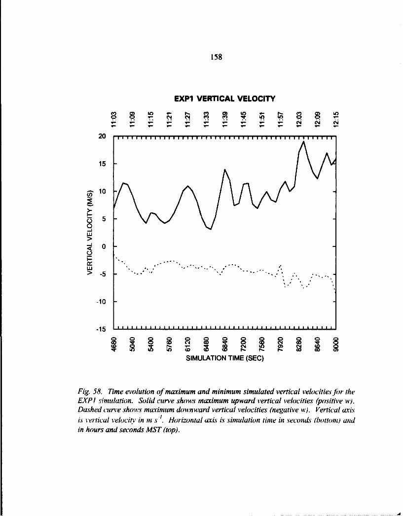
158

EXP1 VERTICAL VELOCITY

0 C% -C% (n) (D) i n W- 0-(nV

20

15

10

0-jLU

<0

> -5

-10

CA N

SIMULATION TIME (SEC)

Fig. 58. Time evolution of maximum and minimum simulated vertical velocitiesoor theEXP I simulation. Solid curve shows maximum upward vertical velocities (positive wt).Dashed curve showts maximum downward vertical velocities (negative i). Vertical axis

is vertical velocity in in s . Horizontal axis is simulation time in se'onds (bottomn andin hours and seconds MST (top).

159

control. Third, the convective initiation occurred much earlier in EXPI than in the

control--4230 s in EXPI compared to 5670 s in the control. The initial calm winds

limited the turbulent transport of heat away from the surface, allowing maximum so-

lar heating and rapid convective development. Fourth, the cells developed between

3.0 and 5.0 km farther east, more directly over the mountain tops, in EXPI than in

the control. Several studies discussed in Chapter 2 (Banta, 1984; Braham and Dragi-

nis, 1960; Glass and Carlson, 1963; Orville, 1965b; Barker and Banta, 1985; Banta

and Schaaf, 1987; Schaaf et al., 1988) described the tendency for leeside convective

development and the mechanisms for such development. In the absence of environ-

mental wind, there is less translation of convective updrafts toward the lee of the

mountains (Orville, 1965b). Thus, under calm wind conditions such as EXPI, it is

natural to expect the storms to develop closer to the mountains than under windier

conditions such as the control. Finally, EXPI's storm developed more steadily and

more slowly than the storm in the control. The reason for this difference in develop-

ment is not entirely clear. The control's more rapid development late in the simu-

lation may be attributed to the relatively strong flow above 6.0 to 8.0 km which

served as an "exhaust mechanism" for the developing cell. This flow helped remove

heat from the top of the cell and the surrounding environment, keepiicg the environ-

mental lapse rate favorable for rapid development. The absence of such a flow in

EXPI may have contributed to its slower, more steady development.

Quantitatively, the storms are markedly different in many respects. The maxi-

mum total condensate mixing ratio evolution shown in Figure 57 shows a rapid rise in

EXPI between 5850 and 6210 s followed by a steady increase through the rest of the

simulation. This development is much different than the extended period of rapid in-

creases in the maximum total condensate mixing ratio seen in the control. Second,

160

the peak total condensate mixing ratio in EXPI reached 6.4 g kg-1 compared to 7.2

g kg'1 in the control. EXPI's pristine ice crystal maximum mixing ratio evolution

differed dramatically from that seen in the control. In EXPI, the maximum mixing

ratio barely reached 5.0 g kg', while in the control, the maximum pristine ice crystal

mixing ratio never went below 5.0 g kgl after 8460 s. The maximum aggregated

snow flake and graupel mixing ratios increase earlier atd persist longer in EXPI than

in the control. All of the maximum mixing ratio traces in Figure 57 show a large

amount of variability not seen in the control. The evolution of maximum updrafts and

downdrafts shown in Figure 58 show a similar amount of variability. The maximum

updrafts exceeded 5.0 m s-' much earlier in EXPI than in the control. EXPI's peak

updraft exceeded the control's by nearly 3.0 m sl, while EXPI's peak downdraft ex-

ceeded the control's by about 1.0 m s-'. Again, the maximum updrafts and down-

drafts indicate a much slower, steadier development in EXPI than in the control.

The marked differences between EXPl's simulation and the control's precluded

any detailed comparison between the two simulations at similar analysis times.

7.3 Experiment 2 - 50% Wind Case

EXP2 was initialized with a wind profile with wind speeds 50% of those in the

control's wind profile. This simulation developed serious boundary condition insta-

bilities which ultimately rendered the simulation useless for the purposes of this study.

The simulation started very much like the control. As early as 5400 s, though, the

first signs of the boundary problems began to appear. By this time a 4.5 m s- easter-

ly flow developed near the eastern model boundary at about 2.5 km. A westerly flow

of 3.0 m s-' had developed at the same boundary at 0.5 kmn. This circulation was ac-

companied by a relatively large negative pressure perturbation (from the base state) in

the low levels near the same boundary.

161

As the simulation progressed, the pressure perturbation and the wind maxima con-

tinued to increase in magnitude. Additionally, strong updrafts and downdrafts devel-

oped and produced extremely large areas of condensate. The spurious circulations

and cells continued to strengthen throughout the simulation. Eventually, the effect of

these disturbances destroyed the credibility of the simulation in the rest of the model

domain.

The cause of the boundary condition problems observed in this simulation are un-

clear. The problem most likely resulted from some reflection or excitation of a cer-

tain wavelength or wavelengths in the model. It is not obvious why the 50% wind

profile produced such disturbances while the stronger winds in the control profile did

not. The problem appears to be related to the topography since it occurs in the lower

levels. However, the topography should have little effect since the initial wind pro-

files for both EXP2 and the control had calm winds below the mountain top.

Chapter 8

Sensitivity To Diabatic Heating Effects

The second two experiments conducted for this study investigated the sensitivity of

the simulated storms to diabatic heating effects. Section 8.1 describes the results of

Experiment 3's (EXP3) simulation. Section 8.2 provides a brief description of the

evolution of Experiment 4's (EXP4) simulated storm and a comparison of the results

with those of the control.

8.1 Experiment 3 - No Short Wave Radiation Case

In EXP3, the simulation was conducted with the RAMS short-wave radiation

package deactivated, effectively "turning off the sun". While no storm developed in

this case, the results provide crucial evidence of the importance of the wind flow in

focusing the convective initiation.

8.1.1 Analysis Of Simulated Cloud Evolution

No convective development occurred during the simulation, however, a small

cloud did develop and persist between 6300 s and 9000 s (Fig. 59). The cloud con-

sisted entirely of cloud water and the maximum mixing ratio never exceeded 0.6

g kg'. A very weak, but steady, updraft of between 2.5 and 3.4 m s- supported the

small cloud. The updraft developed near a quasi-stationary area of low-level conver-

gence located between x = -2.0 and -3.0 km. The convergence resulted from the

interaction of the initial easterly flow with a weak westerly flow below 2.0 km. The

westerly flow appears to have developed as result of a dynamically induced mountain-

wave circulation, perhaps even a rotor circulation, on the lee side of the mountain.

162

163

EXP 3

12~-------------------------------

-------------------------------

I .- - - - - - - - -

F - -8 .0•-4_ .

4 .0ý - - - - - - - -- - -

r2. - - - - - -

-15.0 -10.9 -5.0 0.0 5.0 10.0 15.0

X (KM)

TOTAL CONDENSATE WINDSIN VECTORS

Y = 0.00 KM T = 8460. S

Fig. 59. East-west vertical cross-section of simulated total condensate mixing ratiosoverlaid with simulated wind vectors for EXP3 simulation at 8460 s. Contours are ev-ety 2. 0 g kg-' starting at 0.1 g kg1. Wind vector length shown in lower right-hand cor-

ner of figure equals 50 m s. Vertical axis is labeled in kilometers above the minimumterrain elevation in the simulation grid (in this case 1.82 kin) as described in the text.Horizontal axis is horizontal distance labeled in kilometers. The cross-section shown islocated at y = 0.0 km and runs east-west, with the origin at Langmuir Laborator.

164

Figure 60 shows an example from 7740 s of the convergence described above. A

similar pattern existed well into the simulation to 8460 s.

Both the cloud and the updraft developed between x = -2.0 and -3.0 kin, and re-

mained there through the rest of the simulation. The cloud was located at approxi-

mately z = 2.75 km. A very small secondary cloud developed just to the east of the

first near the end of the simulation.

8.1.2 Comparison With Control

Comparison of the results of EXP3 with those of the control shows several notable

similarities. In both cases, the first clouds formed at nearly the same location. The

cloud developed slightly higher in EXP3 than in the control. Also in both cases, the

cloud and supporting updraft remained nearly stationary for an extended period. In

the control, the stationary cloud and updraft remained in place until the convective

development began to dominate the circulation in the r ea. Finally, both EXP3 and

the control show the development of the quasi-stationary area of low-level conver-

gence induced by the mountain-wave circulation discussed above. This comparison

points out the crucial importance of environmental wind in focusing the convective

initiation.

8.2 Experiment 4 - Warm Rain Microphysics Case

EXP4 was conducted with all the ice-phase microphysical processes deactivated

and only the warm rain purameterizations activated.

8.2.1 Analysis Of Simulated Storm Evolution

Prior to 7920 s, EXP4's development followed exactly or nearly exactly that de-

scribed in Chapter 6 for the control and will not be discussed again here. By 7920 s,

three cells had developed, E4CI near x = -5.0 kin, E4C2 slightly to the east, and

E4C3 near x = 0.0 km. E4CI dominated the simulated storm with total condensate

165

EXP 3

12.0-

S...................... o............. .. o............... .. ................... ................................

-- -- ---.. 0

... . - -.. ... .... .. ............ .

4.9-v 6 .o --... .. .. . . .. .... . ------

- 5.- ...... - .... .. • . 5-.- 1-...1...

X (KM I

WESTERLY WINO

Y = 0.00 KM T = 7740. S

Fig. 60. East-west vertical cross-section of simulated u wind component contoured ev-ery 3.0 m s'1 starting at 1.5 m s-1 for EXP3 simulation at 7740 s. Solid (dashed) con-tours show westerly (easterly) winds. Axes are labeled as in Fig. 59.

166

mixing ratios of up to 3.2 g kg-' and updrafts of 10.0 m s1. E4C2 contained total

condensate mixing ratios in excess of 2.0 g kg-' and updrafts in excess of 4.5 m s-'.

E4C3 contained low total condensate mixing ratios and weak updrafts of about 1.5

m s1. The horizontal flow featured an area of low-level convergence near x = -5.5

km. A rain shaft associated with E4C1 and E4C2 developed between x = -3.5 and

-4.0 km. The peak rain mixing ratio in the storm reached 0.4 g kg-'. The maximum

cloud top at this time reached 5.25 km. Figures 61 and 62 show analyses of total

condensate mixing ratio and vertical velocity, respectively, for 7920 s.

At 8100 s, E4CI continued to dominate the storm with maximum total condensate

mixing ratios of 4.8 g kg-' and maximum updrafts of 13.7 m s-'. E4C2 still contained

total condensate mixing ratios in excess of 2.0 g kgt and updrafts of over 7.5 m s-'.

A significant downdraft of 5.1 m s-' developed at this time between the updrafts asso-

ciated with E4CI and E4C2. E4C3 remained weak with updrafts near 1.5 m s-1 and

low total condensate mixing ratios. The rain shaft widened to about 1.0 km with a

p-.ak storm rain mixing ratio of 1.6 g kg-'. The maximum cloud top reached 5.5 km

by this time.

By 8280 s, both E4CI and E4C2 had weakened slightly. E4CI continued to

dominate with total condensate mixing ratios of 4.8 g kg-1 and a maximum updraft of

10. 1 m s-. E4CI 's updraft showed a double maxima structure with the upper maxi-

mum located near z = 4.5 km and the lower maximum located near z = 2.5 km.

E4C2's total condensate mixing ratio remained slightly above 2.0 g kg' while its up-

draft weakened to about 4.5 m s-1. Meanwhile E4C3 grew slightly in size, but re-

mained at about the same strength as at previous analysis times. The rain shaft

associated with E4CI and E4C2 widened again, this time to nearly 2.0 km. The

167

EXP 4

12.0-_

4 . Z-- - -- - - -

F - - - - - - -

2 .0 ,

• o~ - .. ...1 . . .

• -, I . . . . ' ' ' ' • I I ' I E ', ' ,-

-15.0 -19.6 -5.0 6.0 5.9 16.0 15.0

X (KMI

TOTAL CONDENSATE WINDS

IN VECTORS

Y : 0.00 KM T = 7920. SMIAX tMuM VUTI

Fig. 61. Analogous to Fig. 59, east-west vertical cross-section of simulated total con-densate mixing ratios overlaid with simulated wind vectors Jbr EXP4 simulation at7920 s.

168

EXP 4

1?.j2.0-

-15.0 -10.0 -5.0 0.0 5.0 10.0 15.7X (KM)

VERTICAL WIND

Y = 0.00 KM T = 7920. S

Fig. 62. East-west vertical cross-section of simulated vertical velocity contoured eveiy3.0 m s-1 starting at 1.5 m s'f.br EXP4 simulation at 7920 s. Solid (dashed) contoursshow positive (negative) vertical velocities. Axes labeled as in Fig. 59.

169

maximum storm rain mixing ratio reached 1.9 g kg' in E4CI, and the maximum

cloud top reached 6.25 km.

At 8460 s E4C1 clearly dominated the storm. The cell contained a double maxi-

ma in the totalcondensate mixing ratio. The upper maximum was located at about

5.5 km and contained mixing ratios in excess of 4.0 g kg-t. The lower maximum was

located near 4.0 km and contained mixing ratios of 5.5 g kg-1. The updraft associated

with E4CI increased to 11.8 m s-. Meanwhile, E4C2 continued to weaken with

maximum total condensate mixing ratios dropping below 2.0 g kg' and maximum

updrafts only reaching 1.5 m s-. At the same time, E4C3 developed significantly

over previous analyses with total condensate mixing ratios exceeding 2.0 g kg-' and

maximum updrafts exceeding 4.5 m s-'. The maximum rain mixing ratio in the storm

reached 3.5 g kg-' in E4CI. The rain shaft widened to 2.5 kin, and the maximum

cloud height reached 6.5 km. Figures 63 and 64 show analyses of total condensate

mixing ratio and vertical velocity, respectively, for 8460 s.

The simulation at 8640 s showed that E4CI continued to dominate the storm. Its

maximum total condensate mixing ratio remained nearly steady at 5.4 g kg- I, and its

maximum updraft strengthened to 13.0 m s-1. E4C2 remained relatively weak with

total condensate mixing ratios barely exceeding 2.0 g kg-1 and maximum updrafts of

4.5 m s-1. E4C3 remained at about the same strength as at the previous analysis time,

but grew in size. At this time, a strong mid-level flow out of E4C3, through E4C2,

and into E4CI matured. The rain shaft continued to widen at this time to 3.0 km.

The shaft began to show signs of a split between E4CI and E4C2. The maximum

rain mixing ratio at this time reached 4.4 g kg-1 in E4CI, while the maximum cloud

height remained at 6.5 km.

170

E'-_XP 4

12.ý

------------------------------

F- - - -- - -- - - - -

2 Of

7 . . . . .

-15.0 -10.0 -5.9 9.9 5.0 19.0 15.0

X (KM)

TOTAL CONDENSATE WINDSIN VECTORS

Y = 0.00 KM T = 8460. S

Fig. 63. Analogous to Fig. 59, east-west vertical cross-section of simulated total con-

densate mixing ratios overlaid with simulated wind vectors for EXP4 simulation at8460 s. Contour label "1" represents 0. 1 g kg-1.

171

EXP 4

12.0--

10. On

8.

EAS0

-1. -80 590.0 5.9 10.8 1.5.0

X (K(M)

VERTICAL WIND

Y 0.00 KM T 8460. S

Fig. 64. A nalogo us to Fig. 62, east-west vertical cross-section of simulated vertical ve-bocity for EXP4 simulation at 8460 s..

172

At 8820 s, the condensate from all three cells joined to form a single storm domi-

nated by E4C1. The cell's updraft contained double maxima in both the total conden-

sate mixing ratio field and the updraft. The maximum total condensate mixing ratio

exceeded 4.0 g kg-', and the maximum updraft reached 9.2 m s-1. E4C2 showed little

change in strength from the previous analysis time. A strong downdraft of 5.7 m s-'

developed between the updrafts associated with E4CI and E4C2. E4C3 remained at

about the same strength as in the previous analysis. The rain shaft associated with

E4CI and E4C2 widened to 3.5 km with a split between E4CI and E4C2. The maxi-

mum rain mixing ratio decreased to 3.7 g kg'. The maximum cloud height increased

at this time to 7.0 km.

By 9000 s, E4CI still dominated the storm with a maximum total condensate mix-

ing ratio of 4.9 g kg-t and a maximum updraft of 10.2 m s-. Both of these maxima

were located very near the top of the storm at elevations above 6.0 km. E4C2 be-

came nearly absorbed in E4C1 and E4C3 at this time. E4C3 contained two updrafts

with the strongest exceeding 4.5 m s-1. The maximum total condensate mixing ratio

in E4C3 exceeded 4.0 g kg'. Rain fell out of all three cells at this time, with a maxi-

mum rain mixing ratio of 3.1 g kg-'. The maximum cloud height reached 7.5 km.

Figures 65 and 66 show analyses of total condensate mixing ratio and vertical veloc-

ity, respectively, for 9000 s.

Figures 67 and 68 show the evolution of the simulation's maximum condensate

mixing ratios and upward and downward vertical velocities, respectively.

8.2.2 Comparison With Control

In general, the results of EXP4's simulation were similar to those of the control--

especially given the marked difference in the microphysical parameterizations used.

Prior to 7920 s, EXP4's simulation nearly reproduced exactly that seen in the control.

173

EXP 4

-------------------------

---------------------------------

"- - 1. -. 9.-91.

4.J

2. 9 . -

.- ,0 0

X (KM)

TOTAL CONDENSATE WINDS

IN VECTORS

Y = 0.00 KM T = 9000. S " o.SM-A

Fig. 65. Analogous to Fig. 59, east-west vertical cross-section of simulated total con-densate mixing ratios overlaid with simulated wind vectors for EXP4 simulation at9000 s. Contour label "1" represents 0. 1 g kg-'.

174

EXP 4

12.-

1 6.,;

A.,Iiv,,,

4.0- : 1 ',. 1

-15.0 -10. 0 -5.0 0.0 5.0 16.0 15.9)

X (KM)

VERTICAL WIND

Y 0.00 KM T = 9000..S

Fig. 66. Analogous to Fig. 62, east-west vertical cross-section of simulated vertical ve-locity for EXP4 simulation at 9000 s.

175

EXP4 CONDENSATE MIXING RATIOS

U~~V '- rV c

8

CONDENSATE

-- CLOUD

- - RAIN

Z4

2/

02 1F-- I I' II'/ r-I

SIMULATION TIME (SEC)

Fig. 67. Time evolution of maximum simulated condensate mixing ratios fo•r the EXP4simulation. Solid czuve shows total condensate mixing ratios, dot-dash curve showsukoud water mixing ratios, dashed curve shows rain water mixing ratios, double dlot-dash curve shows pristine ice crystal mixing ratios, shaded curve shoi~w graupel mixingratios, and dotted curve shows aggregated snow flake mixing ratios. Vertical axis ismixing ratio in grams per kilogram. Horizontal axis is simulation time in seconds(hottom) and in hours and seconds MST (top).

176

EXP4 VERTICAL VELOCITY

0 n 0 M- W~0 S - r- 2 0 S

.0. .. ,- W.. T- .. .. -. .. .- . ,,-

15

10

(n

0-J

<00 ...................

-10

SIMULATION TIME (SEC)

Fig. 68. Time evolution of maximum and minimum simulated vertical velocities for theEXP4 simulation. Solid curve shows maximum upward vertical velocities (positive w).Dashed curve shows maximum downward vertical velocities (negative w). Vertical axisis vertical velocit in in s#. Horizontal axis is simulation time in seconds (bottom) andin hours and seconds MST (top).

177

After that time, the two simulations began to differ substantially, but they still gener-

ally corresponded quite well. A comparison of EXP4's condensate mixing ratio

evolution (Fig. 67) with the control's evolution (Fig. 49) shows nearly perfect agree-

ment in the timing of total condensate mixing ratio maxima and minima. Naturally,

the values do not agree quantitatively, but the degree of qualitative agreement is re-

markable. A similar comparison of the vertical velocity evolution (Fig. 68 for EXP4

and Fig. 43 for the control) shows good agreement prior to about 8280 s. After that

time, the correspondence between the two simulations deteriorates with the control's

maximum updrafts and downdrafts exceeding the strength seen in EXP4.

A more detailed comparison of the simulations shows similar results. Prior to

7920 s, very little, if any, distinction could be made between the two simulations.

After that time, several of EXP4's storm characteristics were weaker or less signifi-

cant than the control's. First, EXP4's maximum cloud heights evolved from nearly

the same height as the control's at 7920 s, to 1.0 km lower than the control's at 8460

s, to 2.5 km lower at 8640 s, to 3.5 km lower at 8820 s, and finally to 4.5 km lower

than the control's at 9000 s. During this time period, the ice phases dominated the

development of the storm in the control. In EXP4, the ice phases were not permitted

and thus the development was retarded significantly. Second, the maximum updrafts

in EXP4 were sometimes 5.0 to 7.0 m s-1 weaker than in the control. Similarly,

EXP4's total condensate mixing ratios in many cases were up to 2.0 g kg- less than

in the control. Again, most of these differences can be attributed to the lack of the

ice phases in the simulation. The latent heat release associated with the ice phases

accounted for the most rapid development of the cells in the control during this time

period. Throughout the precipitating phase of EXP4's simulation, the rain shafts

were always narrower and weaker than those observed in the control. This, too, can

178

be attributed to the lack of the ice phases. The rain shafts in the control were very

strongly influenced by the presence of graupel shafts aloft above the rain shafts.

Without the graupel in EXP4, the rain production process did not proceed as efficient-

ly as it did in the control. EXP4's simulated cells did not exhibit the strong total con-

densate mixing ratio maxima found near the top of the control simulation's cells. The

maxima in the control were a direct result of maxima in the ice phases' mixing ratios,

and thus were not a factor in EXP4's simulation. Finally, both E4C2 and E4C3 were

noticeably less significant in EXP4 than their counterparts in the control simulation.

Chapter 9

Sensitivity To Initial Moisture Profile

The final experiment conducted for this study investigated the sensitivity of the

simulated storm to the initial base-state moisture profile. Section 9.1 provides a brief

description of the modified moisture profile used to initialize EXP5. Section 9.2

briefly describes the evolution of EXP5's simulated storm, and Section 9.3 compares

EXP5's results with those of the control.

9.1 Experiment 5 - Moistened Lower Levels Case

EXP5 was designed to test the sensitivity of the simulated storm development to

the initial atmospheric moisture profile. As briefly described in Chapter 5, EXP5's

initial moisture profile was constructed to produce a profile with a higher moisture

content in the lower atmosphere. For this case the initial mixing ratio was increased

in the lowest model levels by 0.5 g kg-1 over that in the control's base-state moisture

profile. The amount of increase over the control was gradually reduced to zero at 720

mb. Above 720 mb, EXP5's initial moisture profile and the control's were identical.

Figure 69 shows EXP5's moisture profile superimposed over the control's.

9.2 Analysis Of Simulated Storm Evolution

By 6840 s, two cells, ESCI near x = -3.0 km and E5C2 near x = -1.0 km, had

developed. E5CI contained a maximum updraft of 5.4 m s-' and a maximum total

condensate mixing ratio of 2.2 g kg-1. The cells' development prior to this time fol-

lowed that of the control with EXP5's development occurring slightly more rapidly

than the control's. For example, by 6840 s, the control's maximum updraft and total

179

180

100 /

200) /

~~~- -4b•• ,, .3W0

S/ ///

700 'p

-20 0 20 40TEMPERATURE (0oQ

Fig. 69. Skew T, log P plot of modified base-state moisture profile used to initialize thenumerical model for the EXP5 simulation. Heavy solid and dashed lines represent sen-sible and dewpoint temperature profiles, respectively. Light dashed line shows originalbase-state moisture profile f)r reference. Skew T, log P diagram labeled as in Fig. 2.

181

condensate mixing ratio reached only 3.2 m sl and 1.2 g kgl, respectively, compared

with EXP5's 5.4 m s-' and 2.2 g kg-'. Figures 70 and 71 show analyses of total con-

densate mixing ratio and vertical velocity, respectively, for 6840 s.

Between 6840 and 7380 s, the storm matured significantly with E5CI dominating

the storm until 7200 s and E5C2 dominating late in the period. The cells exhibited a

degree of the oscillatory development individually and between each other as noted in

the observations described in Chapter 3 and described by Ziegler et al. (1986). ESCI

dominated the storm until 7200 s with maximum updrafts reaching 6.2 m s- at 7020 s

and maximum total condensate mixing ratios reaching 2.6 g kg' at the same time.

These values diminished quickly to about 1.5 in s-I and less than 2.0 g kgt by 7380 s.

A new updraft of about 1.5 m s-1 developed in association with ESCI after 7200 s

near x = -5.0 km. By 7380 s, cloud water, pristine ice crystals, rain, and graupel

had developed in ESCI. As ESCI was weakening late in the period, E5C2 strength-

ened significantly to contain peak updrafts of 5.5 m s-l and total condensate mixing

ratios of 2.4 g kg'. At 7380 s, a new cell (denoted hereafter as E5C3) developed

near x = 1.0 km. Figures 72 and 73 show analyses of total condensate mixing ratio

and vertical velocity, respectively, for 7380 s. During this period, two areas of low-

level convergence developed: one near x = -3.0 km and the other near x = --5.0 km

(Fig. 74). The convergence resulted from the interaction of wind flow patterns simi-

lar to those described in the analysis of the control simulation's evolution.

E5C3 had developed quite rapidly by 7560 s. The cell contained maximum up-

drafts of 10.4 in s1 and a peak total condensate mixing ratio of over 2.0 g kg-'. By

this time, cloud water, pristine ice crystals, graupel, and rain water had developed in

the cell. E5C2 remained relatively unchanged from the previous analysis time with

maximum updrafts of over 4.5 m s1 and maximum total condensate mixing ratios of

182

EXP 5

12."

--- - - - - - -- -- - -- -- - - .- - - - - - - - - - - -

. - . . .-

- - -- - -

4. 0

0.0 . ........2. -•.

X (KM)

TOTAL CONDENSATEIN VECTORS

Y = 0.00 KM - T = 6840. S

Fig. 70. East-west vertical cross-section of simulated total condensate mixing ratiosoverlaid with simulated wind vectors for EXP5 simulation at 6840 s. Contours are ev-ery 2.0 g kg' starting at 0.1 g kg'. Wind vector length shown in lower right-hand cor-

ner o.ffigure equals 50 m s,1. Vertical axis is labeled in kilometers above the minimumterrain elevation in the simulation grid (in this cave 1.82 Imn) as described in the text.Horizontal axis is horizontal distance labeled in kilometers. The cross-section shown islocated at y = 0.0 kon and runs east-west, with the origin at Langmuir Laboratory.

183

EXP 5

X (KM)

VERTICAL WINO

Y = 0.00 KM T = 6840. S

Fig. 71. East-west vertical cross-section of simulated vertical velocit contoured every

3.0 m s-~ starting at 1.5 m s'fipr EXP5 simulation at 6840 s. Solid ('das/zed) contoursvshowt positive (negative) vertical velocities. Axes labeled as in Fig. 70.

184

EXP 5

-. - - - - - - - - - - - - - - - - - - - - - - - -

F - -- -- - - - - -

4 O,ý - -- -- - -

-. 0 -08 -5.0 8.0 5.0 18.0 15.0

X (KM)TOTAL CONDENSATE WINOS

[N VECTORS

Y = 0.00 KM T = 7380. S 9

Fig. 72. Analogous to Fig. 70, east-west vertical cross-section of simulated total c.on-densate mixing ratios overlaid with simulated wind vectors for ExpS sijmulation at7380 Y. Contour label "1 "1represents 0.1I g kg'1.

185

EXP 5

12. 0

2. 0-.

0.0j.

-15.0 -19.0 -51 .0 S.O 10.0 15.0

X (KM)

VERTICAL WIND

Y = 0.00 KM T = 7380. S

Fig. 73. Analogous to Fig. 71, east-west vertical cross-section of simulated vertical ve-locity for EXP5 simulation at 7380 s.

186

EXP 5

12.A-

S....... °.............°....... ....... .. o.. .... .. o.o.. .... o°°o.......o°°....... .................. °......... ....

10.-

& . .................... .......... ...oo ........ . .. ........ .o ......... o .... o .... o ....... o.. .... .......... o.. ......

................................. ..... ........ o oo.o..o...... ......... ......................... o.............

....... .. .......... .50 ..........

r ..... . .. .. ... .. .... ...

I.,

4. 0.-. -2 ....C30

4.•"~ ~ .:-- ,: ......, ,...

--------------- o--o

-15.9 -I,0 -5.0 0.0 5.0 1.9 15.0

X (KM)

WESTERLY WIND

Y 0 00 KM T = 7380. S

Fig. 74. East-west vertical cross-section of simulated u wind component contoured ev-ery 3.0 m s- starting at 1.5 m s'.for EXP5 simulation at 7380 s. Solid (dashed) con-toury show westerly (easterly) winds. Axes are labeled as in Fig. 70.

187

3.0 g kg'. E5CI remained weak with only very weak updrafts and maximum total

condensate mixing ratios of less than 2.0 g kg-'.

By 7740 s, E5C2 clearly dominated the storm with maximum updrafts of 11.8

m s! and peak total condensate mixing ratios of 4.3 g kg-". Graupel developed for

the first time in E5C2 at this time. E5C2 also contained a relatively strong downdraft

of 4.5 m s-. At the same time, E5C3 weakened slightly with a maximum updraft of

7.5 m s'- and maximum total condensate mixing ratios of over 2.0 g kg-. This cell

also contained a downdraft in excess of 4.5 m s-1. E5CI strengthened slightly to in-

clude maximum total condensate mixing ratios of over 2.0 g kg-I.

At 7920 s, E5C3 dominated the storm with a maximum total condensate mixing

ratio of 4.4 g kgl. The cell's updraft contained a double maxima with the upper

maximum (located near 4.0 km) reaching 11.2 m s-1 and the lower maximum (located

near 3.0 kin) reaching over 4.5 m s1. The cell also contained a downdraft of 4.7

m s-'. The first precipitation reached the surface at this time as a rain shaft from

E5C3. E5C2 weakened from the previous analysis time as its updraft split into two

maxima. The upper maximum, located near 4.0 km, exceeded 7.5 m s-, while the

lower maximum, located near 3.0 kin, exceeded 4.5 m s- . The cell's maximum total

condensate still exceeded 2.0 g kg-'. E5CI remained very weak with updrafts still

near 1.5 m S-1 and maximum total condensate mixing ratios dropping below 2.0

g k4-l. Figures 75 and 76 show analyses of total condensate mixing ratio and vertical

velocity, respectively, for 7920 s.

By 8100 s, E5CI showed signs of reintensification while E5C3 weakened dramati-

cally. E5C3 contained maximum updrafts of over 4.5 m s! and maximum total con-

densate mixing ratios of 3.9 g kg-'. Rain continued to fall out of this cell. E5C2

maintained its earlier strength with a maximum updraft in excess of 4.5 m s-1 and

188

EXP 5

12.0--

19.

-15.9 -1- .9 -5.6 6.6 5.- 1-.9 15.9

X (KM)TOTAL CONDENSATE WINOS

IN VECTORS

Y= 0.00 KM T= 7920 S

Fig. 75. East-west vertical cross-section of simulated total condensate mixing ratiosoverlaid with simulated wind vectors, as in Fig. 70, except for EXP5 simulation at 7920s. Contour label "1" represents 0. 1 g kgt.

189

EXP 5

12. 9-

4.0-

2 .0--0.m

- -10 ,.0 -5.0 9.0 5.0 10.0 1 .

X (KM IVERTICAL WIND?

Y = 0.00 KM T = 7920. S

Fig. 76. East-west vertical cross-section of simulated vertical velocity as in Fig. 71.except.for EXP5 simulation at 7920 s.

190

maximum total condensate mixing ratios of over 2.0 g kg-1. The first precipitation

developed out of E5C2 at this time as a rain shaft. Meanwhile, E5CI's maximum

updraft increased to 7.5 m s- while its maximum total condensate mixing ratio re-

mained below 2.0 g kg'. The maximum cloud top reached 6.0 km at this time. The

ice phases began to dominate at this time as E5C2 pushed into the colder air at these

higher levels. E5CI's intensification at this time resulted from the intensification of

the low-level convergence near x = -5.5 km. This intensification was accompanied

by a gradual weakening of the convergent area nearx = -3.0 km (Fig. 77).

ESCI continued to develop rapidly at 8280 s with maximum updrafts of 12.2 n s-'

and maximum total condensate mixing ratios exceeding 2.0 g kg-'. The first preci-

pitation from E5CI developed as a rain shaft at this time. Also, the first graupel de-

veloped in the cell at this time. All of E5CI's condensate became very closely

merged with that of E5C2 at this time. E5C2's strength remained nearly steady with

peak updrafts in excess of 4.5 m s-l and a maximum total condensate mixing ratio of

4.4 g kg-'. The condensate maximum occurred near the top of the cell and consisted

primarily of pristine ice crystals. The first aggregated snow flakes of the simulation

developed near this maximum at this time. Rain continued to fall from E5C3, but its

maximum updraft decreased to just over 1.5 m s-1 while its maximum total condensate

mixing ratio dropped below 2.0 g kg8". At the same time, graupel from the cell near-

ly reached the surface and some weak development of aggregated snow flakes oc-

curred near the top of the cell.

By 8460 s, E5CI's updraft dominated the storm with a maximum value of 14.8

Ss-1. The cell's maximum total condensate mixing ratio continued to remain above

2.0 g kgl. E5C2 contained a double maxima updraft with the upper maximum ex-

ceeding 7.5 m s-1 and the lower maximum exceeding 4.5 m s-1. The cell's maximum

191

EXP 5

12.1-

.............. ...--...-." " 1-11°-- ...... o....°....... .... .......................... ........---............

r6..............o.. ....... ........ °...... ........-.......... .... .... .... .. ..... ...... ..... ............ .......

........ ..................... ---------- ................." .......... ..°°. ...° ...o ....o ............ .-- o.o o....

8."

z-1.i --S. .........

.,..................................I...........

S...." ", • .:..•_ .... , )0" ............=4.~~~-t ........... ..............."..,.."• ". o

2 0 ......................... ..... .,.........,- '-:::::::::

---------- -

2.• ":::'--2-

-15.0 -0.9 -S.0J 6.6 5.0 16.6 15.6

X IKM)

WESTERLY WIND

Y =. 0.00 KM T = 8100. S

Fig. 77. East-west vertical cross-section of simulated u wind component as in Fig. 74except.for EXP5 simulation at 8100 s.

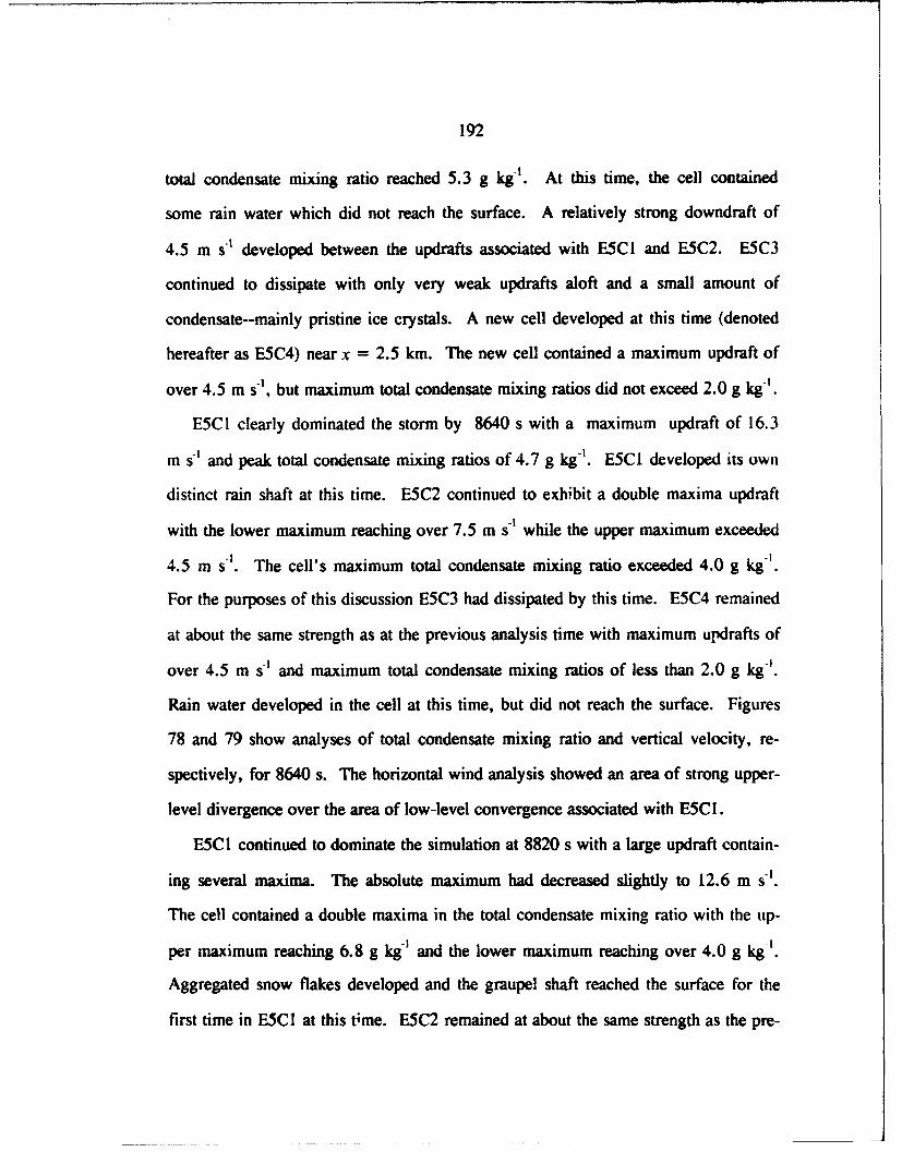
192

total condensate mixing ratio reached 5.3 g kg-1. At this time, the cell contained

some rain water which did not reach the surface. A relatively strong downdraft of

4.5 m s" developed between the updrafts associated with E5CI and E5C2. E5C3

continued to dissipate with only very weak updrafts aloft and a small amount of

condensate--mainly pristine ice crystals. A new cell developed at this time (denoted

hereafter as E5C4) near x = 2.5 km. The new cell contained a maximum updraft of

over 4.5 m s1, but maximum total condensate mixing ratios did not exceed 2.0 g kg-'.

E5C1 clearly dominated the storm by 8640 s with a maximum updraft of 16.3

in s-1 and peak total condensate mixing ratios of 4.7 g kgl. E5CI developed its own

distinct rain shaft at this time. E5C2 continued to exhibit a double maxima updraft

with the lower maximum reaching over 7.5 m s-1 while the upper maximum exceeded

4.5 m s-1. The cell's maximum total condensate mixing ratio exceeded 4.0 g kg'.

For the purposes of this discussion E5C3 had dissipated by this time. E5C4 remained

at about the same strength as at the previous analysis time with maximum updrafts of

over 4.5 m s-' and maximum total condensate mixing ratios of less than 2.0 g kg-'.

Rain water developed in the cell at this time, but did not reach the surface. Figures

78 and 79 show analyses of total condensate mixing ratio and vertical velocity, re-

spectively, for 8640 s. The horizontal wind analysis showed an area of strong upper-

level divergence over the area of low-level convergence associated with E5CI.

E5CI continued to dominate the simulation at 8820 s with a large updraft contain-

ing several maxima. The absolute maximum had decreased slightly to 12.6 m s-'.

The cell contained a double maxima in the total condensate mixing ratio with the up-

per maximum reaching 6.8 g kg-' and the lower maximum reaching over 4.0 g kg-'.

Aggregated snow flakes developed and the graupel shaft reached the surface for the

first time in E5CI at this t;me. E5C2 remained at about the same strength as the pre-

193

EXP 5

12. --1---------------------K - - -

S. ... ........!. .... ....2. ,

0. Ii r I I I I I ) I ! I | I

-15.0 -10.0 -5.0 0.0 5.0 10.0 15.0

X (KM)

TOTAL CONDENSATE WINOS

IN VECTORS

Y = 0.00 KM T = 8640. S

Fig. 78. Analogous to Fig. 70, east-west vertical cross-section of simulated total con-densate mixing ratios overlaid with simulated wind vectors for EXP5 simulation at8640 s. Contour label "1" represents 0. 1 g kg'.

194

EXP 5

12.-

100. 1..

8.•-

2. Vo

8.-

-15.9 -19.9 -5.9 U.9 5.9 1@.9 15.9

X (KM)

VERTICAL WIND

Y = 0.00 KM T = 8640. S

Fig. 79. Analogous to Fig. 71, east-west vertical cross-section of simulated vertical ve-locity for EXP5 simulation at 8640 s.

195

vious analysis time with peak updrafts of over 7.5 m s-1. The cell contained several

total condensate mixing ratio maxima with most of them over 4.0 g kg-'. E5C4 con-

tinued to intensify with peak updrafts reaching over 7.5 m s-1 and maximum total con-

densate mixing ratios of over 2.0 g kg'. Pristine ice crystals and graupel developed

in E5C4 at this time.

By the end of the simulation at 9000 s, ESCI continued to dominate the storm.

The cell contained several updraft maxima with the strongest peaking at 14.6 m s-'.

The maximum total condensate mixing ratio reached 7.1 g kg' near the top of the

cell. The aggregated snow flake mixing ratio increased to over 2.0 g kg' for the first

time. E5C2 weakened slightly with a maximum updraft continuing to exceed 7.5

m s- , but with the maximium total condensate mixing ratio dropping to just over 2.0

g kg-'. E5C4 remained at about the same strength as before with updrafts in excess of

4.5 m s-1 and maximum total condensate mixing iatios of over 2.0 g kg-'.

Figures 80 and 81 show the evolution of the simulation's maximum condensate

mixing ratios and upward and downward vertical velocities, respectively.

9.3 Comparison With Control

Given the relatively small change in the initial moisture profile, the results of

EXP5's simulation differed dramatically from those of the control. EXP5's simu-

lation produced four cells compared to three cells in the control. The first three cells

to develop in EXP5 developed in generally the same locations as their counterparts in

the control. The development of these cells differed dramatically from those in the

control. While the western-most cell (ESCI in EXP5 and CCI in the control) ulti-

mately dominated the simulation in both cases, in EXP5, this domination was preced-

ed by strong development of E5C2 and E5C3. In fact, the rapid development of

E5C3 seemed to retard for a time the development of the two cells to its west. The

196

EXP5 CONDENSATE MIXING RATIOS

V - C4 N. C 4,

10 *, i a i * i i i I i i i i i i i i i i i i i i i i i i i i i i i i i ii i I

I CONDENSATE8

--..-- CLOUD

-. - - -- RAIN

c 6 ----- PRISTINE h.0 GRAUPEL/

-AGGREGATEIZ 4X

2

%- 04 4'I

3 , n co.,-rI, -.- - /.. , -i

SIMULATION TIME (SEC)

Fig. 80. Time evolution of maximum simulated condensate mixing ratios for the EXP5simulation. Solid curve shows total condensate mixing ratios, dot-dash curve showscloud water mixing ratios, dashed curve shows rain water mixing ratios, double (lot-dash curve shows pristine ice crystal mixing ratios, shaded curve show's graJpel mixingratios, and dotted curve shows aggregated snow flake mixing ratios. Vertical axis ismixing ratio in grams per kilogram. Horizontal axis is simulation time in seconds(bottom) and in hours and seconds MST (top).

197

EXP5 VERTICAL VELOCITY

M r~I- p Q , r

V- 1r T- `1 - V- V- T- V- W- C 1

20

15 -

10

I,- S50-j

.J<0

> -

-10

-15 ri v lo 1ity i 1 i 1 1 Ho r I i z o I I sl I mN lati on tu e 1 1 a of I N o I I I

SIMULATION TIME (SEC)

Fig. 81. Time evolution of maximum and minimum simulated vertical velocities for theEXP5 simulation. Solid curve shows maximum upward vertical velocities (positive w).Dashed curve shows maximum downward vertical velocities (negative %v). Vertical axisis• vertical velocity in m s-1. Horizontal axis is simulation time in seconds (hottom) andin hours and seconds MST (top).

198

circulation and cool downdrafts associated with E5C3 inhibited the flow of warm,

moist air into the cells to its west, thus slowing their development. E5C2 maintained

its strength much longer into the simulation than its counterpart cell in the control.

A comparison of EXP5's maximum condensate ratio evolution (Fig. 80) with the

control's evolution (Fig. 49) shows several differences. First, EXP5's development

appears steadier, and did not reach its absolute maximum total condensate mixing ra-

tio until the end of the simulation. The early development (before 8280 s) produced

higher total condensate mixing ratios in EXP5 than in the control. Second, EXP5's

rain water mixing ratios were slightly higher early in the simulation and then lagged

those of the control by up to 1.0 g kg-I later in the simulation. EXP5's peak graupel

mixing ratios were higher much earlier than in the control. The pristine ice crystal

mixing ratios in both cases followed about the same development pattern with a rapid

increases between 7920 s and 8280 s.

A similar comparison of the vertical velocity evolution (Fig. 81 for EXP5 and

Fig. 43 for the control) shows general agreement in the upward trend of updraft

strength. The comparison shows little correspondence between the timing of the

maxima and minima in the updrafts of both simulations. The absolute maximum for

EXP5 was about 4.0 m sm greater than in the control. A comparison of the downdraft

time series shows generally good agreement between both simulations.

A more detailed comparison of the simulations shows similar results. Prior to

7560 s, the simulations in both EXP5 and in the control were very similar. The dif-

ferences were minor with EXP5's updrafts slightly stronger than the control's and the

maximum total condensate mixing ratio in EXP5 reaching peaks about 0.5 g kg'

greater than the control's between 6840 and 7560 s. Between 7560 and 7920 s, E5C3

developed very rapidly and even began producing precipitation. The corresponding

199

cell in the control, CC3, showed only very weak development during this period.

EXP5's two western cells, E5CI and E5C2, still were not producing precipitation by

7920 s, while the merged storm in the control was producing precipitation by this

time. Between 8100 and 8460 s, as E5C3 diminished, the pattern of the merged

storm in EXP5 appeared very similar to that in the control. The major difference

during this period was that in EXP5, the dominant cell was E5C2, the eastern cell,

while in the control, the dominant cell was CCI, the western cell. The updrafts and

maximum total condensate mixing ratios for the two simulations agreed reasonably

well during this period. During the period from 8640 to 9000 s, the maximum cloud

tops in EXP5 were consistently lower than those in the control. The difference

ranged from 0.75 km at 8640 s to 1.75 km at 8820 s. Also during this time, both

ESCI and E5C2 attained approximately the same height while in the control, CC1

grew to much higher levels than did CC2.

Chapter 10

Conclusions

This research examined the initiation, development, and maintenance of a small

mountain thunderstorm using numerical simulations. The storm considered in this

study occurred on 31 July 1984 and is typical of the many storms which form each

summer in and around the Magdalena Mountains of central New Mexico. As a result

of their frequency and relatively fixed location, the storms have been studied exten-

sively for at least the past 15 years. The current study examines the 31 July 1984

storm using the two-dimensional, non-hydrostatic cloud model configuration of the

Colorado State University Regional Atmospheric Modeling System (Tripoli and Cot-

ton, 1982, 1986; Cotton et al., 1982, 1986; Tripoli, 1986). The study also employs

the multiple Doppler analyses performed by Lang (personal communication, 1992)

following the technique of Ray etal. (1981) and described in detail by Lang (1991) as

well as the three-dimensional microphysical retrieval performed by Lang (1991) for a

similar storm that occurred on 3 August 1984.

The numerical model was used to isolate the processes and initial conditions most

important in the initiation, development, and maintenance of these types of storms. A

total of six simulations were conducted--one control and five experiments. The re-

sults of the control sinI.•-ion were compared with Doppler analyses and with Lang's

(1991) retrieval to assess the validity of the simulation and its usefulness in studying

the storm. The experiments were conducted to test the sensitivity of the simulated

storms to initial wind profile, the lack of solar heating, restriction to warm rain

200

201

processes, and the initial moisture profile. The results of these simulations were com-

pared with the control's results.

Analyses of the Doppler radar observations and synthesized wind fields provided

the basis for evaluating the accuracy of the control numerical simulation. The analy-

ses showed that early cell development occurred directly over or slightly east of the

ridge lines. Convective initiation was favored in these locations by upslope flow

through convergent valleys located on the eastern and southeastern slopes of the

mountain. As the storm developed, circulations from existing cells affected the initia-

tion locations of new cells. For example, several short-lived cells developed along

the outflow boundaries from older cells, and in some cases the low-level flow induced

by the existing cells enhanced or created upslope and/or convergent flows which in

turn helped focus new cell development.

The observed storms generally had lifetimes of 1.0 to 1.5 hr with individual cell

lifetimes ranging from 20 to 60 min. Many of the cells exhibited periodic intensifica-

tion and weakening with a period of 6 to 12 min. Radar returns from the strongest

cells exceeded 50 dBZ several times, but maximum returns from most cells ranged

from 30 to 40 dBZ. Most cells never extended higher than 10.0 km MSL, however,

the strongest cells frequently extended to over 12.0 km MSL. Most cells contained

single updrafts approximately 2.0 km wide with maximum vertical velocities of 12.0

m s-1 or less, however, the strongest updrafts reached 18.0 m s-1. At least one cell

contained multiple low-level updrafts which merged into a single updraft at mid-

levels. Mature cells contained downdrafts with large areal coverages and maximum

vertical velocities frequently exceeding 6.0 m s- with an absolute maximum of 12.0

m s-. During one cell's mature stage, the interaction between the updraft and the

downdraft appeared to be symbiotic in a manner similar to that often observed in

202

long-lived severe storms. In this case, the precipitation and its associated downdraft

were located behind and below the updraft (relative to the low-level inflow) and thus

did not interfere with the inflow or the updraft.

A strong interrelationship existed between all the cells in the analysis domain. In

the mature stage, the outflow from downdrafts appeared in some cases to enhance

low-level convergence that either focused the development of new cells or helped sus-

tain existing cells. In several instances the updrafts of two or more cells merged into

one updraft at upper-levels. Often the updraft of a newer cell developed in the low-

to mid-levels and fed into a higher-level updraft associated with an older cell. The

periodic intensification noted above appeared to alternate among the cells. In other

words, when one cell intensified, the others weakened slightly. Finally, the observa-

tions showed several cases where older or weaker cells were overtaken and absorbed

by newer and/or stronger cells.

Comparison of the evolution of the control's simulated storm with observations

and with Lang's (1991) microphysical retrieval show that the simulation accurately

captured the major features observed by the radars and accurately depicted the micro-

physical evolution of the storm cells. In fact, given the limitations imposed by the

use of a single initialization sounding and the two-dimensional nature of the simu-

lation, the simulation performed above expectations. The simulation accurately de-

picted the development of a multi-cellular storm with horizontal and vertical

dimensions very similar to those observed. The simulation captured low-level inflow

and convergence regions as well as upper-level outflow regions. In general, the

strength of the simulated cells was close to that observed by the radars. The imposed

limitations did, however, introduce several discrepancies between the simulation and

the observations. These included an initial delay in convective development of about

203

20-30 min from that observed; more rapid development than observed; slightly stron-

ger updrafts and weaker, less-organized downdrafts than observed; a tendency for de-

velopment farther west than observed; and the development of an upper-level total

condensate mixing ratio maximum with no corresponding maximum in the radar re-

flectivity fields.

The simulated microphysical evolution compared favorably with that described by

Lang (1991). In particular, the simulation accurately depicted the importance of

warm rain processes early in the cell development and the subsequent rapid increase

in the importance of the ice phase processes. The simulation also differed from the

retrieval results in several areas. The simulated mixing ratios of ice crystals and ag-

gregated snow flakes were much higher than those retrieved, while the simulated rain

mixing ratios were much lower than those retrieved. Additionally, the maximum

simulated rain mixing ratio occurred after the graupel maximum, while in the retriev-

al, the rain maximum occurred first.

The first two experiments tested the sensitivity of the simulated storm to the initial

wind profile. The first experiment, EXPI, used an initial wind profile consisting of

calm winds throughout the depth of the atmosphere. Comparison of the results of this

simulation with those of the control shows that the initial wind profile plays an impor-

tant role in the initiation and evolution of the simulated storms. The simulated cells

in EXPI developed directly over the ridge lines instead of to the west of the ridges as

in the control. The location of cell development in EXPI is more consistent with the

observed cell development than is the control. EXPI's storm cells developed earlier,

but grew at a slower, steadier pace than the control's. EXPI's initially calm winds

limited the turbulent transfer of heat away from the surface, allowing maximum solar

heating and rapid convective development. The control's more rapid growth may be

204

attributed to a relatively strong flow at mid- to upper-levels which served as an "ex-

haust mechanism" for the developing cells. EXPI's storm contained two cells of

nearly equal strength and height through most of the development period. The reason

for this difference from the control was riot clear. Finally, EXPI's microphysical and

vertical velocity evolution showed a much greater variability than that seen in the con-

trol.

The results of EXP1 showed that the initial wind profile strongly influences the

rate of development of all cells and may even inhibit the development of some cells.

The wind profile also exerts influence over the microphysical evolution and vertical

velocity evolution of the storm. Finally, the initial wind profile plays a significant

role in the convective initiation location.

The second experiment, EXP2, was initialized with a wind profile containing

wind speeds 50% of those in the control. This simulation developed serious boundary

condition instabilities which rendered the simulation useless for the purposes of this

study.

The third experiment, EXP3, was conducted with the model's short-wave radi-

ation package deactivated to test the effect on the simulated storm of a "no sun" sce-

nario. In this simulation, very small, non-convective clouds form at nearly the same

locations as the initial clouds in the control--slightly west of the ridge. A weak, but

steady, updraft supported the clouds. The updraft developed near a nearly stationary

area of low-level convergence which resulted from interaction of the predominantly

easterly flow with a weak westerly flow near the surface. The westerly flow devel-

oped as a result of a dynamically induced mountain wave circulation on the lee side of

the mountain. The results of this simulation show that solar heating plays the most

important role in the development of these mountain thunderstorms. The results of

205

this experiment combined with those of EXPI also show that the environmental wind

field plays a crucial role in determining the convective initiation locations.

The fourth experiment, EXP4, tested the sensitivity of the simulated storm to a

restriction to warm rain microphysical processes. In this experiment all the model's

ice phase microphysical parameterizations were deactivated. The results from early in

this simulation agreed very well with those of the control. Later in the simulation

EXP4's results showed the simulated storm contained weaker updnrifts and lower total

condensate mixing ratios. Additionally, the cells did not extend as high as those in

the control. EXP4's rain shafts were much weaker than in the control, and the total

condensate mixing ratio maxima noted near the cell tops in the control were much

weaker in EXP4. The good early agreement between the results of this experiment

and those of the control confirm the importance of warm rain processes in the storm's

early development. The growing differences between the two simulations show that

as the storm matured, the ice phases became increasingly important to the evolution of

the storm's development. Indeed, the absence of the ice phase processes and their

associated latent heat release processes in EXP4 prevented the storm from reaching

the strengths achieved in the control. The lack of the efficient precipitation-producing

mechanisms associated with the ice phases prevented the rain shafts in EXP4 from

reaching the strengths achieved in the control. This experiment demonstrated the im-

portance of the ice phases in the development of these mountain storms--particularly

in their middle to late stages of development.

The final experiment, EXP5, tested the sensitivity of the simulated storms to the

initial base-state moisture profile. The initial moisture profile in this case was moist-

ened by up to 0.5 g kg* in the lowest 1.0 km. This simulated storm generally fol-

lowed that of the control, however, one of the very minor cells in the control

206

dominated EXP5's simulation for a time. In general EXP5's simulated storm devel-

oped at a steadier pace than the control and eventually contained stronger updrafts and

higher graupel mixing ratios than the control. EXP5's cells did not reach the same

heights as the control's, and as in EXPI, two cells developed to nearly the same

strength. This experiment clearly shows the importance of low-level moisture to the

evolution of these mountain storms. In particular, the moisture profile seemed to in-

fluence the ability of some cells to develop beyond cumulus stages. Additional low-

level moisture contributes to stronger updrafts and slightly higher condensate mixing

ratios, but interestingly does not increase the height of the cells. The lower cloud

heights may be attributed to the increase in the number of larger cells. The increased

competition among the larger cells may prevent any of them from reaching the heights

seen in the control.

In summary, the results of the numerical simulations showed the following condi-

tions and processes to be most important (in descending order) to the development and

maintenance of the mountain storms under study here: solar heating, ice phase micro-

physical processes, environmental wind profile, and low-level moisture profile. The

environmental wind profile was the single most important factor in the convective ini-

tiation location.

The most obvious limitation of the simulations conducted for this study was their

two-dimensional nature. This limitation prevented a detailed quantitative analysis of

the validity of the control simulation compared with the Doppler analyses. It also

prevented the simulation from capturing the channelling of the wind flow up the vari-

ous valleys in the Magdalena Mountains. The observations demonstrate the impor-

tance of this phenomenon in focusing the convective initiation and in contributing to

the maintenance of the storm development.

207

Future studies of this nature should attempt to overcome these limitations by em-

ploying fully three-dimensional simulations. The three-dimensional simulations

should also be conducted with larger domains so as to further minimize the boundary

condition effects on the areas of interest such as those noted in EXP2. Future studies

should also attempt to employ higher resolution grid systems in both the horizontal

and vertical directions. A higher resolution grid system will naturally require a high-

er resolution input terrain field. Such high resolution grids will minimize the need for

extensive parameterizations of processes so important to the development of these

small storms.

Comparison of numerical simulation results with Doppler analyses would be

markedly simplified with the employment of a technique to synthesize radar reflectivi-

ties based on the simulated microphysical storm structure. Finally, the accuracy of

three-dimensional simulations could be improved with improved initial conditions.

This study used a single profile to initialize the simulation. A complex four-

dimensional data assimilation system using all available data including Doppler radar

observations and perhaps retrieved microphysical parameters could provide the model

with a significantly more realistic representation of the base-state atmosphere. With

further model developments, such high-quality analyses could provide information

required to "nudge" the simulation as it is progressing toward a more realistic solu-

tion.

REFERENCES

Anderson, C.E., 1960: A study of the pulsating growth of cumulus clouds. Geopkys-ical Research Papers, No. 72, Air Force Cambridge Research Laboratories, 136PP.

Bader, D.C. and T.B. McKee, 1983: Dynamical model simulation of the morningboundary layer development in deep mountain valleys. J. Clim. Appi. Meteor., 22,341-351.

Bader, D.C. and T.B. McKee, 1985: Effects of shear, stability and valley characteris-tics on the destruction of temperature inversions. J. Clim. AppL. Meteor., 24,822-832.

Bader, D.C., T.B. McKee, and G.J. Tripoli, 1987: Mesoscale boundary layer evolu-tion over complex terrain. Part I: Numerical simulation of the diurnal cycle. J.Atmos. Sci., 44, 2823-2838.

Banta, R.M., 1983: A boundary-layer-scale model of mountain upslope flow. Pre-prints, Sixth Conference on Numerical Weather Prediction, Omaha, American Me-teorological Society, Boston, 328-334.

Banta, R.M., 1984: Daytime boundary-layer evolution over mountainous terrain. PartI: Observation of the dry circulations. Mon. Wea. Rev., 112, 340-356.

Banta, R.M., 1986: Daytime boundary-layer evolution over mountainous terrain. PartII: Numerical studies of upslope flow duration. Mon. Wea. Rev., 114, 1112-1130.

Banta, R.M. and C.B. Schaaf, 1987: Thunderstorm genesis zones in the ColoradoRocky Mountains as determined by traceback of geosynchronous satellite images.Mon. Wea. Rev., 115, 463-476.

Barker, C.L. and R.M. Banta, 1985: Preferred regions of thunderstorm initiation overthe Colorado Rockies. Preprints, 14th Conference on Severe Local Storms, In-dianapolis, Indiana, American Meteorological Society, Boston, 17-20.

Battan, Louis J., 1973: Radar Ubservation of the Atmosphere. University of ChicagoPress, Chicago, IL, 324 pp.

Braham, R.R. and M. Draginis, 1960: Roots of orographic cumuli. J. Meteor.. 17,214-226.

208

209

Browning, K.A., J.C. Fankhauser, J.-P. Chalon, P.J. Eccles, R.G. Strauch, F.H.Merrem, D.J. Musil, E.L. May, and W.R. Sand, 1976: Structure of an evolvinghailstorm, Part V: Synthesis and implications for hail growth and hail suppression.Mon. Wea. Rev., 104, 603-610.

Chen, C. and W.R. Cotton, 1983: A one-dimensional simulation of thestratocumulus-capped mixed layer. Boundary-Layer Meteorol., 25, 289-321.

Clark, T.L., 1977: A small scale dynamic model using a terrain-following coordinatetransformation. J Comp. Physics, 24, 186-215.

Clark, T.L. and R. Gall, 1982: Three-dimensional numerical model simulations ofairflow over mountainous terrain: A comparison with observations. Mon. Wea.Rev., 110, 766-791.

Cotton, W.R., M.A. Stephens, T. Nehrkorn, and G.J. Tripoli, 1982: The ColoradoState University three-dimensional cloud/mesoscale model--1982. Part II: An icephase parameterization. J. Rech. Atmos., 16, 295-320.

Cotton, W.R. and G.J. Tripoli, 1978: Cumulus convection in shear flow--Three-dimensional numerical experiments. J. Atmos. Sci., 35, 1503-1521.

Cotton, W.R., G.J. Tripoli, R.M. Rauber, and E.A. Mulvihill, 1986: Numericalsimulation of the effects of varying ice crystal nucleation rates and aggregationprocesses on orographic snowfall. J. Clim. AppL Meteor., 25, 1658-1680.

Defant, F., 1951: Local winds. Compendium of Meteorology, T.M. Malone, Ed.,American Meteorological Society, 655-672.

Durran, D.R., 1981: The effects of moisture on mountain lee waves. Ph. D. Dis-sertation, Massachusetts Institute of Technology and National Center for Atmo-spheric Research, Cooperative Thesis No. 65, 142 pp.

Dye, J.E., B.M. Ruiz, J.J. Jones, W.P. Winn, W. Williams, J.W. Bullock, B.A.Miller, and D.J. Younkin, 1987: The onset of electrification in New Mexico thun-derstorms. Preprints, 23rd Conference on Radar Meteorology, Snowmass, CO,American Meteorological Society, 153-156.

Gal-Chen, T. and R.C.J. Somerville, 1975a: On dhe use of a coordinate transforma-tion for the solution of the Navier-Stokes equations. J. Comp. Physics, 17,209-228.

Gal-Chen, T. and R.C.J. Somerville, 1975b: Numerical solution of the Navier-Stokesequations with topography. J. Comp. Physics, 17, 276-310.

Glass, M. and T.N. Carlson, 1963: The growth characteristics of small cumulusclouds. J. Atmos. Sci., 20, 397-406.

Hill, G.E., 1974: Factors controlling the size and spacing of cumulus clouds as re-vealed by numerical experiments. J. Atmos. Sci., 31, 646-673.

210

Joss, J. and D. Waldvogel, 1970: Raindrop size distributions and Doppler velocities.Preprints, 14th Conference on Radar Meteorology, Tuscon, AZ, American Meteo-rological Society, 153-156.

Kessler, E. I11, 1969: On the Distribution and Continuity of Water Substance in At-mospheric Motions. Meteorological Monographs, No. 32, American Meteorologi-cal Society, Boston, 84 pp.

Klemp, J.B. and R.B. Wilhelmson, 1978a: The simulation of three-dimensional con-vective storm dynamics. J. Atmos. Sci., 35, 1070-1096.

Klemp, J.B. and R.B. Wilhelmson, 1978b: Simulations of right- and left-movingstorms produced through storm splitting. J. Atmos. Sci., 35, 1097-1110.

Lang, S.E., 1991: Retrieving microphysical variables in a small mountain thunder-storm. M. S. Thesis, Florida State University, Tallahassee, FL, 269 pp.

Lilly, D.K., 1962: On the numerical simulation of buoyant convection. Tellus, 14,148-172.

Liu, J.Y. and H.D. Orville, 1969: Numerical modeling of precipitation and cloudshadow effects on mountain-induced cumuli. J. Atmos. Sci., 26, 1283-1298.

Louis, J.-F., 1979: A parametric model of vertical eddy fluxes in the atmosphere.Boundaiy-Layer Meteorol., 17. 187-202.

Manton, M.J. and W.R. Cotton, 1977: Parameterization of the atmospheric surfacelayer. J. Atmos. Sci., 34, 331-334.

McCumber, M.C. and R.A. Pielke, 1981: Simulation of the effects of surface fluxesof heat and moisture in a mesoscale numerical model. 1. Soil layer. J. Geophys.Res., 86, 9929-9938.

McCutchan, M.H. and D.G. Fox, 1986: Effect of elevation and aspect on wind, tem-perature, and humidity. J. Clim. Appl. Meteor., 25, 1996-2013.

Ogura, Y., 1962: Convection of isolated masses of buoyant fluid: a numerical cal-culation. J. Atmos. Sci., 19, 492-502.

Orville, H.D., 1964: On mountain upslope winds. J. Atmos. Sci., 21, 622-633.

Orville, H.D., 1965a: A numerical study of the initiation of cumulus clouds overmountainous terrain. J. Atmos. Sci., 22, 684-699.

Orville, H.D., 1965b: A photogrammetric study of the initiation of cumulus cloudsover mountainous terrain. J. Atmos. Sci., 22, 700-709.

Orville, H.D., 1968: Ambient wind effects on the initiation and development of cu-mulus clouds over mountains. J. Atmos. Sci., 25, 385-403.

211

Paegle J., W.G. Zdunkowski, and R.M. Welch, 1976: Implicit differencing of pre-dictive equations of the boundary layer. Mon. Wea. Rev., 104, 1321-1324.

Ray, P.S., C.L. Ziegler, W. Bumgarner, and R.J. Serafin, 1980: Single- andmultiple-Doppler radar observations of tornadic storms. Mon. Wea. Rev., 106,1607-1625.

Raymond, D.J. and M. Wilkening, 1980: Mountain-induced convections under fairweather conditions. J. Atmos. Sci., 37, 2693-2706.

Raymond, D.J. and M. Wilkening, 1982: Flow and mixing in New Mexico mountaincumuli. J. Atmos. Sci., 39, 2211-2228.

Raymond, D.J. and M. Wilkening, 1985: Characteristics of mountain-induced thun-derstorms and cumulus congestus clouds from budget measurements. J. Atmos.Sci., 42, 773-783.

Schaaf, C.B., J. Wurman, and R.M. Banta, 1988: Thunderstorm-producing terrainfeatures. Bull. Amer. Meteor. Soc., 69, 272-277.

Schlesinger, R.E., 1975: A three-dimensional numerical model of an isolated deepconvective cloud: Preliminary results. J. Atmos. Sci., 32, 934-957.

Schlesinger, R.E., 1978: A three-dimensional numerical model of an isolated thun-derstorm: Part I. Comparative experiments for variable ambient wind shear. J.Atmos. Sci., 35, 690-713.

Scorer, R.S., 1958: Natural Aerodynamics. Pergamon Press, New York, NY, 312Pp.

Scorer, R.S. and F.H. Ludlam, 1953: Bubble theory of penetrative convection.Quart. J. Roy. Meteor. Soc., 79, 94-103.

Smolarkiewicz, P.K. and T.L. Clark, 1985: Numerical simulation of the evolution ofa three-dimensional field of cumulus clouds. Part I: Model description comparisonwith observations and sensitivity studies. J. Atmos. Sci., 42, 502-522.

Srivastava, R.C., 1967: A study of the effect of precipitation on cumulus dynamics.J. Atmos. Sci., 24, 36-44.

Tapp, M.C. and P.W. White, 1976: A non-hydrostatic mesoscale model. Quart. J.Roy. Meteor. Soc., 102, 277-296.

Todd, C.J., 1964: Aircraft traverses in a growing mountain cumulus cloud. J. Atmos.Sci., 21, 529-538.

Toth, J.J. and R.H. Johnson, 1985: Summer surface flow characteristics over north-east Colorado. Mon. Wea. Rev., 113, 1458-1469.

212

Tremback, C.J. and R. Kessler, 1985: A surface temperature an moisture parameter-ization for use in mesoscale numerical models. Preprints, Seventh Conference onNumerical Weather Prediction, Montreal, Canada, American Meteorological Soci-ety, 355-358.

Tremback, C.J., G.J. Tripoli, and W.R. Cotton, 1985: A regional scale atmosphericnumerical model including explicit moist physics and a hydrostatic time-splitscheme. Preprints, Seventh Conference on Numerical Weather Prediction, Mon-treal, Canada, American Meteorological Society, 433-434.

Tripoli, G.J., 1986: A numerical investigation of an orogenic meso-scale convectivesystem. Ph. D. Dissertation, Atmos. Sci. Paper No. 401, Colorado State Univer-sity, Ft. Collins, CO, 290 pp.

Tripoli, G.J. and W.R. Cotton, 1980: A numerical investigation of several factorscontributing to the observed variable intensity of deep convection over south Flori-da. J. Appl. •leteor., 19, 1037-1063.

Tripoli, G.J. and W.R. Cotton, 1981: The use of ice-liquid water potential tempera-ture as a thermodynamic variable in deep atmospheric models. Mon. Wen. Re%.,109, 1094-1102.

Tripoli, G.J. and W.R. Cotton, 1982: The Colorado State University three-dimensional cloud/mesoscale model--1982. Part 1: General theoretical frameworkand sensitivity experiments. J. Rech. Atmos., 16, 185-219.

Tripoli, G.J. and W.R. Cotton, 1986: An intense, quasi-steady thunderstorm overmountainous terrain, Part IV: Three-dimensional numerical simulation. J. Attmos.Sci., 43, 894-912.

Tripoli, G.J., P.J. Flatau, and W.R. Cotton, 1988: Generalized microphysics schemefor use in mesoscale/cloud models. Preprints, 10th International Cloud PhysicsConference, 15-20 August 1988, Bad Homburg, FRG.

Turner, J.S., 1962: The "starting plume" in neutral surroundings. J. Fluid Mech.,13, 356-368.

Winn, W.P., G.W. Schweda, and C.B. Moore, 1974: Measurements of electric fieldsin thunderclouds. J. Geophys. Res., 79, 1761-1767.

Ziegler, C.L., P.S. Ray, and D.R. MacGorman, 1986: Relations of kinematics, mi-crophysics, and electrification in an isolated mountain thunderstorm. J. .4tlos.Sci., 43, 2098-2114.

BIOGRAPHICAL SKETCH

Mark Edwin Raffensberger was born on 9 January 1961 in York, Pennsylvania.

Mark graduated in June of 1979 from Dallastown Area High School in Dallastown,

Pennsylvania. From 1979 to 1983 he attended the Pennsylvania State University

campuses in York and State College, Pennsylvania and graduated with a Bachelor of

Science degree in meteorology in May of 1983. After completing Officer Training

School in November of 1983, Mark was commissioned in the United States Air Force

and assigned to Hill Air Force Base in Utah where he served as Staff Meteorologist

for the Utah Test and Training Range. He began his graduate work in the Air Force

Institute of Technology Civilian Institutions program at Florida State University in the

fall of 1986. After completing his coursework in 1988, he was transferred to Air

Weather Service Headquarters at Scott Air Force Base, Illinois, where he managed

Air Force weather research and development programs while simultaneously complet-

ing his thesis requirements for graduate school.

Mark has co-authored a paper presented in 1989 at the 24th Conference on Radar

Meteorology in Tallahassee, Florida based on material from his master's thesis. He

will continue his work in numerical modeling in the Simulations and Techniques

branch at the United States Air Force Environmental Technical Applications Center at

Scott Air Force Base, Illinois, where he was transferred in August of 1993.

213