numerical simulation of underexpanded sonic jet

NUMERICAL SIMULATION OF UNDEREXPANDED SONIC JET

Malsur Dharavath and Debasis Chakraborty

Directorate of Computational Dynamics

Defence Research and Development Laboratory

Kanchanbagh Post

Hyderabad - 500 058, India

Email : [email protected]

Abstract

Underexpanded sonic jet is numerically simulated using commercial CFD software. Three

dimensional Navier Stokes equations alongwith two equation turbulence models are solved.

Computed centerline distribution and profiles of various flow variables at various axial

stations agree quantitatively with experimental results. The comparison of the flow variables

computed with four different two equation models reveals that k - ε and RNG k - ε models

perform very well in predicting both pressure and temperature throughout the flow filed;

whereas SST and k - ω models fail to predict the flow behavior beyond the first Mach disc.

Introduction

Sonic and supersonic jets are of interest from the point

of view of fundamental fluid mechanics as well as practi-

cal applications. Underexpanded sonic jets are often used

in high-performance nozzles of missiles and rockets,

scramjet combustor, chemical lasers etc. A thorough

knowledge of the global structure and the dynamics of

these flows are important in the future development of air

and space propulsion systems. Better understanding of the

jet structure can lead to reduced thermal signature and jet

noise. The underexpanded sonic jet is treated as a canoni-

cal problem in the literature and efforts are continuing to

have better understanding of its structure.

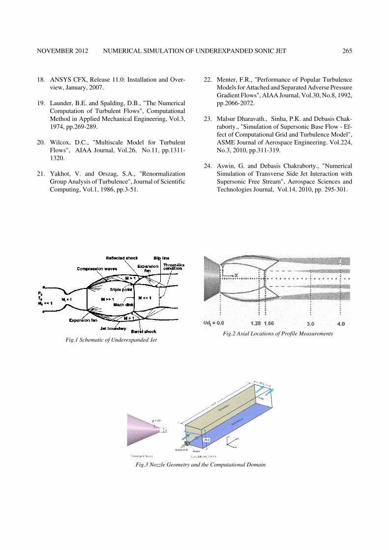
The schematic of the underexpanded sonic jet flow

field is shown in Fig.1. The underexpanded jet flowfield

contains viscous and inviscid regions, normal and oblique

shocks, and regions of expansion and compression waves.

As the static pressure at jet exit is greater than the ambient

pressure, flow at the exit of the jet is accelerated by the

Prandtl-Meyer expansion fan centered at the lip of the jet

nozzle. In the downstream, the atmospheric constant pres-

sure boundary redirects the expansion waves towards the

jet centerline as a series of compression waves which in

turn coalesce to form the oblique intercepting shock. This

barrel-like shock, separating the inner jet core from the

outer sheath of supersonic fluid, terminates at the Mach

disk. The outer jet region persists downstream of the Mach

disk and the near-field shock system repeats itself down-

stream, forming a number of weaker shock cells. The

compressible shear layer at the outer edge of the jet grows

with downstream distance and the jet eventually transit to

a fully-developed turbulent stream in the far field.

The underexpanded jet flowfield has been studied

theoretically, experimentally and computationally since

last few decades. Englert [1] used series solution to pro-

vide an operational method for determining the initial

contour and pressure field about a supersonic jet. Previous

numerical studies often relied on the method of charac-

teristics (MOC) [2-4] for determining the inviscid jet

velocity field, centreline Mach number distribution and

Mach disk location as a function of stagnation pressure

over a range of flow conditions in both sonic and super-

sonic underexpanded jets. Measurements in sonic/super-

sonic jets are difficult because of nonsuitability of direct

measurement method, due to varying static pressure, high

velocities and shocks. Nonintrusive flow measurement

techniques, namely Laser Doppler Anemometry and Laser

Induced Fluorescence have been employed to measure

various flow parameters in the underexpanded jet [5-9].

Woodmansee, Dutton and Lucht [10] used high-resolution

N2 CARS technique to obtain mean pressure, temperature,

and density measurements in the flowfield of an underex-

panded jet. Time averaged CARS measurements have

been acquired along the centerline and for radial traverses

at a number of streamwise locations in the underexpanded

Paper Code : V64 N4/771-2012. Manuscript received on 23 Jan 2012. Reviewed and accepted as a Full Length Contributed Paper

on 03 Sep 2012

jet flowfield. Reliable measurement of velocity and turbu-

lent quantities of the underexpanded jet is still very limited

for the validation of computational model.

With the advent of powerful computer and advanced

numerical techniques, CFD methods have become ma-

tured and are increasingly being used in aerospace designs

and in complex flow physics exploration. Various Euler

[11] and Parabolised Navier Stokes (PNS) [12, 13] meth-

ods are employed in the simulation of underexpanded jet

and these methods overpredict the shock structure and

underpredict the mixing rate. NavierStokes calculations

[14] with k-ε turbulence model showed promising results

to capture the underexpanded jet flow structure. Birkby

and Page [15] used Navier Stokes equations and k-ε tur-

bulence model with compressibility corrections to simu-

late underexpanded jet flow field using a pressure based

methodology. Their simulations predict correct shock -

cell wavelength but decay was too rapid compared to the

experimental results. The comparison of Fluorescence

Imaging of underexpanded jet by Wilkes et al. [16] with

CFD results from GASP (General Aerodynamic Simula-

tion Program) [17] revealed that although for lower jet

pressure ratios, the jet primary wave length agrees with the

experimental results but for higher pressure ratio, the

computed Mach disk diameter and Mach disk location

differ from the experimental results by 35% and 15 %

respectively. It is clear that underexpanded jets need to be

analyzed in greater detail and the role of various turbu-

lence models need to be studied for accurate prediction of

the jet characteristics.

In this work, experimental condition of Woodmansee

et al. [10] is simulated numerically and the centerline

distribution and radial profiles at different cross sections

of various flow parameters are compared with experimen-

tal values. The capabilities of different two equation tur-

bulence models were also assessed in predicting the radial

profiles of underexpanded sonic jet.

Experimental Condition for Which the Simulation is

Carried Out

The present simulation explore the experimental con-

dition of Woodmansee et al. [10] where the center line and

radial profiles of mean pressure, temperature, and density

of an underexpanded jet is measured using a high-resolu-

tion N2 CARS technique. The underexpanded jet flowfield

is generated using a converging nozzle attached to a high-

pressure flow system. Upstream of the converging nozzle,

the stagnation temperature and pressure are measured. The

jet facility is moved with respect to the stationary probe

volume, instead of translating the CARS probe volume to

different positions in the jet flowfield. The jet operating

conditions are summarized in Table-1. The jet with a

Reynolds number of 1.31 x 105 is operated with a nozzle

pressure ratio (Pt/ p∞) of 6.17. The relatively large convec-

tive Mach number (Mc = 0.8), shows that the shear layer

experienced substantial compressibility effect. Upstream

of the Mach disk, the CARS centerline measurement

locations are spaced by 356 µm, whereas the spacing

between the measurement locations is doubled in the

downstream of the Mach disc. The radial profiles are

measured at locations corresponding to x /dj of 0.0, 1.28,

1.56, 3.0, and 4.0 as shown in Fig.2. The profile locations

are chosen so that jet structure near nozzle exit, mach disk

and the farfield region could be clearly distinguished.

Computational Methodology

CFX-10 [18] is an integrated software system capable

of solving diverse and complex multidimensional fluid

flow problems. The software solves three dimensional

Reynolds Averaged Navier Stokes (RANS) equations in a

fully implicit manner. It is a finite volume method and is

based on a finite element approach to represent the geome-

try. The method retains much of the geometric flexibility

of finite element methods as well as the important conser-

vation properties of the finite volume method. The soft-

ware has four major modules a) CFX Build, imports CAD

geometry or creates geometry and generates unstructured

volume meshing based on the user input b) preprocessor

- sets up the boundary condition and initial field condition

c) solver manager - solves the flow field based on the grid

and the boundary condition and d) postprocessor - visual-

izes and extracts the results. It utilizes numerical upwind

schemes to ensure global convergence of mass, momen-

tum, energy and species. In the present study, the discreti-

Table-1 : Inflow Parameters for Underexpanded Jet

Parameters Values

Jet stagnation pressure (Pt) [atm] 6.05

Jet stagnation temperature [K] 296

Jet Reynolds Number (Rej) [million] 0.13

Convective Mach Number (Mc) 0.8

Nozzle exit diameter (d) [mm] 5.0

Nozzle convergent angle (deg) 20

Free stream pressure (p∞) [atm] 0.98

Free stream temperature [K] 294

260 JOURNAL OF AEROSPACE SCIENCES & TECHNOLOGIES VOL.64, No.4

sation of the convective terms is done by second order

upwind difference scheme. Local time stepping has been

used to obtain steady state solutions. Baseline calculations

are done with k-ε turbulence model [19] with wall func-

tion. Three different two-equation turbulence turbulence

models namely k-ω [20] and SST [21], RNG based k-εturbulence model [22] are also simulated for assessing the

predictive capabilities of these models in predicting un-

derexpanded jet structures. In RNG k-ε model, the dissi-

pation rate transport equation models the rate of strain rate

that may be important for the treatment of nonequilibrium

flows and flows in rapid distortion limit such as massively

separating flow and stagnation flow. To find out the accu-

racy and the range of applications, the software has been

validated extensively for various complex flows including

supersonic base flows [23], transverse injection in super-

sonic flow for missile control [24] etc and very good

quantitative agreement with the experimental results are

obtained The details of governing equations, turbulence

models and the discretisation schemes are given in the

following subsections.

Governing Equations

The appropriate system of equations governed the

turbulent compressible gas may be written as

Continuity equation :

∂ ρ∂ t

+ ∂

∂ xk

(ρ uk ) = 0 k = 1 ,2 ,3

Momentum equation :

∂∂ t

(ρ ui ) +

∂∂ x

k

(ρ ui u

k) +

∂ p

∂ xi

= ∂(τ

ik)

∂ x i

, i, k = 1, 2, 3

Energy equation :

∂∂ t

(ρ E ) + ∂

∂ xk

(ρ uk H) = −

∂∂ x

k

(uj τ

jk) +

∂ qk

∂ xk

, j, k = 1, 2, 3

where, ρ , ui , p , E and H are the density, velocity com-

ponents, pressure and total energy and total enthalpy re-

spectively Turbulent shear stress is defined as

τik

= µ

∂ ui

∂ xk

+ ∂ u

k

∂ xi

µ = µ l + µ t is the total viscosity ; µ l , µt being the laminar

and turbulent viscosity

Laminar viscosity (µ l) is calculated from Sutherland law

as

µ l = µ

ref

T

Tref

3⁄2

Tref

+ S

T + S

where, T is the temperature and µref , Tref and S are known

coefficient.

In eddy viscosity models, the stress tensor is expressed

as a function of turbulent viscosity (µ t). Based on dimen-

sional analysis, few variables (k, ε, ω) are defined as given

below,

Turbulent kinetic energy k,

k = u′i u′

i

_____ ⁄ 2

Turbulent dissipation rate ε,

ε ≡ v ∂ u′

i

∂ xj

∂ u′i

∂ xj

+ ∂ u′

j

∂ xi

Specific dissipation rate ω,

ω = εk

The turbulent viscosity µ i is calculated as

µ i = cµ

ρ k2

ε

The heat flux qk is calculated as qk = − λ ∂ T

∂ xk

, λ is the

thermal conductivity

k-ω Turbulence Model

The turbulent viscosity is calculated as function of k

and ω [20].

µ i = f

ρk

ω

NOVEMBER 2012 NUMERICAL SIMULATION OF UNDEREXPANDED SONIC JET 261

Turbulent kinetic energy (k) equation :

∂∂ t

(ρ k) + ∂

∂ xi

(ρ kui) =

∂∂ x

j

Γk ∂ k

∂ xj

+ Gk − Y

k

Specific dissipation rate (ω) equation :

∂∂ t

(ρ ω) + ∂

∂ xi

(ρ ωui) =

∂∂ x

j

Γω ∂ ω∂ x

j

+ Gω − Yω

Where Gk, Yk, Γk and Gω, Yω, Γω are the production,

dissipation and diffusion terms of the k and ω equations

respectively.

SST Turbulence Model

To retain the robust and accurate formulation of Wil-

cox’s k-ω model in the near wall region, and to take

advantage of the freestream independence of the k-εmodel in the outerpart of the boundary layer, Menter [21]

blended both the models through a switching function. k-εmodel was transformed into Wilcox’s k-ω formulation

and was multiplied by (1-F1) and added to original k-ωmodel multiplied by F1 . The blending function F1 will be

one in the near wall region and zero away from the surface.

.In the second step, the definition of eddy viscosity was

modified in the following way to account for the

vt =

a1 k

max (a1 ω ; Ω F

2)

transport of the principal turbulent shear stress

(τ = − ρ u′ v′_______

)

Renormalized Group (RNG) k-ε Model

An improved method for rapidly strained flows based

on rigorous statistical technique [22] is also used in the

present calculations. The k and ò equations are given

below :

∂∂ t

(ρ k) + ∂

∂ xi

(ρ kui) =

∂∂ x

j

αk µ

eff

∂ k

∂ xj

+ Gk − ρ ò − Y

M

∂∂ t

(ρ ò) + ∂

∂ xi

(ρ òui) =

∂∂ x

j

αò µ

eff

∂ ò

∂ xj

+ C1 ò

× ò

k × G

k − C

2 ò ρ

ò2

k − R

ò

Where Gk is the generation of turbulence kinetic energy

due to the mean velocity gradients, calculated as

Gk = − ρu′i u′j_____

∂ uj

∂ xi

and YM represents compressibility

effects given by, YM = 2 ρ ò Mt 2

. The turbulent Mach

number Mt is given by Mt = √k ⁄ a2.

The model constants are taken as,

C1ò = 1.42 , C2ò = 1.68 , Cµ = 0.0845 , σk = σò = 1.393

The additional term in ε equation Rε is given as

Rò =

Cµ ρ η3 (1 − η ⁄ η

o )

1 + β η3

ò

2

k ,

where η ≡ Sk / ò, ηo = 4.38 and β = 0.012.

Discretisation of Governing Equations

The CFX-TASCflow solver utilizes a finite volume

approach, in which the conservation equations in differen-

tial form are integrated over a control volume described

around a node, to obtain an integral equation. The pressure

integral terms in momentum integral equation and the

spatial derivative terms in the integral equations are evalu-

ated using finite element approach. An element is de-

scribed with eight neighboring nodes. The advective term

is evaluated using upwind differencing with physical ad-

vection correction. The set of discretised equations form

a set of algebraic equations: A x→ = b where x→ is the

solution vector. The solver uses an iterative procedure to

update an approximated xn (solution of x at nth

time level)

by solving for an approximate correction x′ from the equa-

tion A x′→

= R→

, where R→

= b→

− A x→n is the residual at

nth

time level. The equation A x′→

= R→

is solved approxi-

mately using an approach called Incomplete Lower Upper

factorization method.

Results and Discussions

Taking the advantage of the symmetry of the flowfield,

only one quadrant of the flowfield is simulated. The nozzle

geometry and the computational domain are shown in

Fig.3. The X, Y and Z axes are taken along the longitudi-

nal, height and lateral directions respectively and the ori-

gin is taken at the centerline of the nozzle at the exit plane.

The computational domain is extended to 103 times the

nozzle diameter (103d) in the longitudinal direction and

20d in the both lateral and height direction. The free stream


inflow plane is placed at 4d upstream of the nozzle exit

plane. A Very fine structured grid of 3.7 million size (292

x 90 x 85) is generated in the flowfield. To capture the

initial growth of the jet very fine mesh are employed near

the inflow and the centerline. The grids are made progres-

sively coarser as we proceed downstream and the far field

boundary. The typical computational grid is shown in

Fig.4. Grid independence of the results are studied by

carrying out the simulation with another grid of 1.84

million size (240 x 90 x 85) and comparing the results.

(Grid independence of the results are discussed later).

Stagnation pressure (6.05 atm) and stagnation temperature

(296K) are specified in the convergent section of the

nozzle and free stream pressure (0.98 atm) and tempera-

ture (294 K) are specified in the free stream inflow plane.

Pressure and supersonic boundary conditions are pre-

scribed for the farfield and outflow boundaries respec-

tively. A log normalized residue of 10-6

is considered as

the convergence criteria for mass, momentum and energy

equations.

The qualitative features of the flow field are depicted

through the Mach number and temperature distributions

in the symmetry plane of the flow field in Fig.5. All the

essential features of the flow field including Mach discs,

barrel shocks, shock cells are crisply captured in the simu-

lation. Computed centerline distribution of pressure, tem-

perature and pressure profile at x/D =4.0 are compared for

two different grids and experimental values in Fig.6. It can

be observed that by changing the grid from 1.84 million

to 3.67 million the results do not vary significantly thus

demonstrating the grid independence of the results.

Simulations are carried out with four different two

equation turbulence models namely, (1) k-ε (2) k-ω (3)

SST and (4) RNG k-ε to assess their capabilities in simu-

lating underexpanded jet. The axial distributions of cen-

terline pressure and temperatures with different turbulence

models are compared with experimental results Figs.7a

and 7b respectively. A very good comparison is obtained

between the experimental and numerical values obtained

with k-ε and RNG k-ε models . The computed locations

of the first two Mach discs match extremely well with the

experimental data. Downstream of the second recompres-

sion region (x/D > 3.5) the computed pressure data show

a plateau, while the experimental data is showing wavy

trend. The maximum difference of computed and experi-

mental pressure values are of the order of 10% (same as

the experimental uncertainty as reported in Ref.10). All

turbulence models captured the overall trend of the experi-

mental results. The k-ε and RNG k-ε models followed the

similar pattern throughout the computational length and

match the experimental pressure extremely well. The SST

and k-ω models show higher pressure beyond x/d > 2.0.

SST model could not predict centerline temperature be-

yond x/D > 3.

The pressure profiles at x/d = 0, 1.28, 1.56, 3.0 and 4.0

are compared between experimental and different turbu-

lence model in Fig.8. It is observed in the figures that upto

the first shock cell (Upto x/d =1.28), all the turbulence

models showing the similar trend. But downstream of the

first Mach disc, SST and k-ω models fail to capture the

experimental trends. Both k-ε and RNG k-ε models pre-

dict the experimental pressure profiles reasonably well

upto x/d = 3.0. In the last axial station (x/d = 4.0), none of

the turbulence models in able to predict centerline vari-

ation of the pressure. At the nozzle exit (Fig.8a, although

trend of the pressure profile is captured, computed pres-

sure under predict the experimental value by about 12%.

In the middle of the first shock cell, the jet structure is well

behaved and the computations agree very well with the

experimental value. In the recompression region of 1st

Mach disc (Fig.8c), the computation captures the experi-

mental trend reasonably well, although the crest and valley

of the experimental pressure is higher than the computa-

tional result in the zone (0 < y/d < 0.4). At X/d =3.0,

(Fig.8d) the comparison is very good except the dip in

experimental pressure at y/D = 0.7. The computation could

not capture the pressure profile at the second Mach disc

location at x/D =4.0 (Fig.8e). Although the jet width is

captured, computed pressure profile is showing a plateau

region compared to intense shock interactions in the cen-

terline region. The cause of this mismatch could not be

explained. The experimental temperature profiles at the

same axial stations are compared with different turbulence

model in Fig.9. Temperature profiles are seen to match the

experimental values quite nicely. Maximum deviations

between the computed and the experimental values with

k-ε turbulence model are of the order 10 K. Turbulence

models exhibit similar trends for temperature prediction

also. Both k-ε and RNG k-ε models predict the experimen-

tal temperature profiles for all the axial stations; while the

performance of SST and k-ω models are not statisfactory

for the prediction the temperature profiles for axial sta-

tions downstream of the first Mach disc.

Conclusions

Numerical explorations are carried out for underex-

panded sonic jet using commercial CFD solvers. Three


dimensional Navier Stokes equations are solved alonwith

two equation turbulence model. Simulation captures all

the essential flow features including Mach discs, barrel

shocks etc. Very good match has been obtained with

experimental data for centerline distribution of all the

variables. Computed temperature profiles match very

nicely with the experimental values at different axial sta-

tions. Although, pressure profiles at near field axial loca-

tions match nicely with the experimental values, some

deviations are observed for the core pressure in the farfield

axial stations. Four different turbulence models were stud-

ied to assess their predictive capabilities for underex-

panded sonic jet and all the turbulence models predicts the

profiles and centerline values of pressure and temperature

upto the first Mach disc very well. Both k-ε and RNG k-εmodels predict the experimental temperature profiles for

all the axial stations very well, but the performance of SST

and k-ω models are not very good in predicting tempera-

ture and pressure profiles in the far field region beyond

first Mach disc.

References

1. Englert, G.W., "Operational Method of Determining

Initial Contour of and Pressure Field about a Super-

sonic Jet", NASA TND 279, 1960.

2. Adamson, T.C., Jr, and Nicholls, J.A., "On the Struc-

ture of Jets from Highly Underexpanded Nozzles into

Still Air", Journal of Aerospace Sciences, Vol 26,

No.1, 1959, pp.16-24.

3. Fox, J.H., "On the Structure of Jet Plumes", AIAA

Journal Vol.12, No.1, January 1974, pp.105-107.

4. Abbett, M., "The Mach Disk in Underexpanded Ex-

haust Plumes", AIAA Journal, Vol.9, No.3, March

1971, pp.512-514.

5. Adrian, R. J., "Laser Velocimetry", in Fluid Mechan-

ics Measurements, R.J. Goldstein, ed., Taylor and

Francis, 1996, pp.175-293.

6. Eggins, P.L. and Jackson, D.A., "Laser- Doppler

Velocity Measurementsin an Under-Expanded Free

Jet", Journal of Physics D: Applied Physics, Vol.7,

1974, pp.1894-1906.

7. Krothapalli, A., Buzyna, G. and Lourenco, L.,

"Streamwise Vortices in an Underexpanded Axisym-

metric Jet", Physics of Fluids A, Vol.3, No.8, 1991,

pp.1848-1851.

8. Chuech, S.G., Lai, M.C. and Faeth, G.M., "Structure

of Turbulent Underexpanded Free Jets", AIAA Jour-

nal, Vol.27, 1989, pp.549-559.

9. Wilkes, J.A., Glass, C.E., Danehy, P.M. and Nowak,

R. J., "Fluorescence Imaging of Underexpanded Jets

and Comparison with CFD", AIAA Paper No. 2006-

910, 2006.

10. Woodmansee, M. A., Dutton, J.C. and Lucht, R.P.,

"Experimental Measurements of Pressure, Tempera-

ture, and Density in an Underexpanded Sonic Jet

Flowfield, AIAA Paper No.99-3600, 1999.

11. Matsuda, T., Umedy, Y., Ishii, R., Yasuda, A. and

Sawada, K., "Numerical and Experimental Studies

on Choked Underexpanded Jets" AIAA Paper

No.87-1378, 1987.

12. Dash, S. M., Wolf, D.E. and Seiner, J.M., "Analysis

of Turbulent Underexpanded Jets, Part-1: Parabol-

ized Navier - Stokes Model, SCIPVS", AIAA Jour-

nal, Vol.23, No.4, April 1985, pp.505-514.

13. Abdol-Hamid, K.S. and Wilmoth, R.G., "Multiscale

Turbulence Effects in Underexpanded Supersonic

Jet", AIAA Journal, Vol.27, 1989, pp.315-322.

14. Cumber, P.S., Fairweather. M., Falle, S.A.E.G. and

Giddings, J.R., "Predictions of the Structure of Tur-

bulent, Moderately Underexpanded Jets", Trans.

ASME, Journal of Fluid Engineering, Vol.116, 1994,

pp.703-713.

15. Birkby, P. and Page, G.J., "Numerical Predictions of

Turbulent Underexpanded Sonic Jets Using a Pres-

sure-based Methodology", Proceedings of IME - Part

G - Journal of Aerospace Engineering, 2001, Vol.215

(3), pp.165-173

16. Wilkes, J.A., Glass, C.E., Danehy, P.M. and Nowak,

R.J., "Fluorescence Imaging of Underexpanded Jets

and Comparison with CFD", AIAA 2006-910.

17. GASP Version 4.0 User’s Manual, Aerosoft, Inc.,

Blacksburg, VA, 2002, ISBN 09652780-5-0.


18. ANSYS CFX, Release 11.0: Installation and Over-

view, January, 2007.

19. Launder, B.E. and Spalding, D.B., "The Numerical

Computation of Turbulent Flows", Computational

Method in Applied Mechanical Engineering, Vol.3,

1974, pp.269-289.

20. Wilcox, D.C., "Multiscale Model for Turbulent

Flows", AIAA Journal, Vol.26, No.11, pp.1311-

1320.

21. Yakhot, V. and Orszag, S.A., "Renormalization

Group Analysis of Turbulence", Journal of Scientific

Computing, Vol.1, 1986, pp.3-51.

22. Menter, F.R., "Performance of Popular Turbulence

Models for Attached and Separated Adverse Pressure

Gradient Flows", AIAA Journal, Vol.30, No.8, 1992,

pp.2066-2072.

23. Malsur Dharavath., Sinha, P.K. and Debasis Chak-

raborty., "Simulation of Supersonic Base Flow - Ef-

fect of Computational Grid and Turbulence Model",

ASME Journal of Aerospace Engineering. Vol.224,

No.3, 2010, pp.311-319.

24. Aswin, G. and Debasis Chakraborty., "Numerical

Simulation of Transverse Side Jet Interaction with

Supersonic Free Stream", Aerospace Sciences and

Technologies Journal, Vol.14, 2010, pp. 295-301.

Fig.1 Schematic of Underexpanded JetFig.2 Axial Locations of Profile Measurements

Fig.3 Nozzle Geometry and the Computational Domain


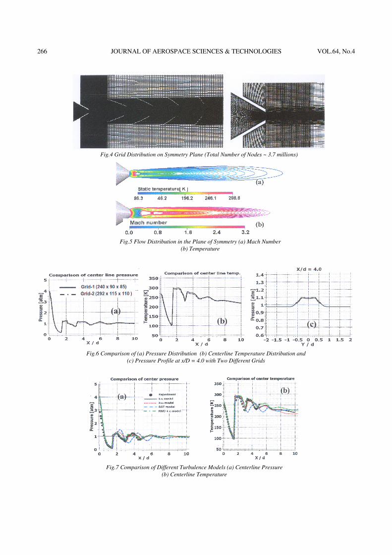
Fig.4 Grid Distribution on Symmetry Plane (Total Number of Nodes ~ 3.7 millions)

Fig.5 Flow Distribution in the Plane of Symmetry (a) Mach Number

(b) Temperature

Fig.6 Comparison of (a) Pressure Distribution (b) Centerline Temperature Distribution and

(c) Pressure Profile at x/D = 4.0 with Two Different Grids

Fig.7 Comparison of Different Turbulence Models (a) Centerline Pressure

(b) Centerline Temperature


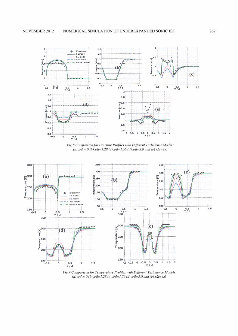
Fig.8 Comparison for Pressure Profiles with Different Turbulence Models

(a) x/d = 0 (b) x/d=1.28 (c) x/d=1.56 (d) x/d=3.0 and (e) x/d=4.0

Fig.9 Comparison for Temperature Profiles with Different Turbulence Models

(a) x/d = 0 (b) x/d=1.28 (c) x/d=1.56 (d) x/d=3.0 and (e) x/d=4.0


numerical simulation of underexpanded sonic jet

Documents