numerical simulation of two-phase solid-liquid slush flows ... · politecnico di milano laurea...
TRANSCRIPT
POLITECNICO DI MILANO
LAUREA MAGISTRALE ING. AERONAUTICA
VON KARMAN INSTITUTE FOR FLUID DYNAMICS
NUMERICAL SIMULATION OF TWO-PHASE SOLID-LIQUIDSLUSH FLOWS FOR PROPULSION SYSTEMS
RUBEN DI BATTISTA
Supervisor: Prof. Luciano GalfettiCo-Supervisor: Prof. Maria Rosaria Vetrano (Von Karman Institute for Fluid Dynamics)Co-Supervisor: Prof. Jean-Marie Buchlin (Von Karman Institute for Fluid Dynamics)

A mio padre, mia madre e mio fratello
ρ = |tanϕ||cotϕ|
Indice
Abstract 9
Sommario 11
1 Introduction 131.1 Classification of slurries . . . . . . . . . . . . . . . . . . . . . . . . . . . . . . . . . . . . . . . 14
1.1.1 Stokes number . . . . . . . . . . . . . . . . . . . . . . . . . . . . . . . . . . . . . . . . 17
2 State of the Art 192.1 Production Techniques . . . . . . . . . . . . . . . . . . . . . . . . . . . . . . . . . . . . . . . . 19
2.1.1 Auger method . . . . . . . . . . . . . . . . . . . . . . . . . . . . . . . . . . . . . . . . . 192.1.2 Freeze-thaw method . . . . . . . . . . . . . . . . . . . . . . . . . . . . . . . . . . . . . 20
2.2 Experimental Setups . . . . . . . . . . . . . . . . . . . . . . . . . . . . . . . . . . . . . . . . . 212.2.1 Density Measurements . . . . . . . . . . . . . . . . . . . . . . . . . . . . . . . . . . . 212.2.2 Flow rate measurements . . . . . . . . . . . . . . . . . . . . . . . . . . . . . . . . . . 232.2.3 Heat Transfer Measurements . . . . . . . . . . . . . . . . . . . . . . . . . . . . . . . 23
2.3 Handling . . . . . . . . . . . . . . . . . . . . . . . . . . . . . . . . . . . . . . . . . . . . . . . . 242.3.1 Piping . . . . . . . . . . . . . . . . . . . . . . . . . . . . . . . . . . . . . . . . . . . . . 242.3.2 Heat leaks and pressure oscillations . . . . . . . . . . . . . . . . . . . . . . . . . . . 252.3.3 Pressurization . . . . . . . . . . . . . . . . . . . . . . . . . . . . . . . . . . . . . . . . . 252.3.4 Aging . . . . . . . . . . . . . . . . . . . . . . . . . . . . . . . . . . . . . . . . . . . . . . 25
3 Numerical Modeling 273.1 Eulerian Two-Fluid Model . . . . . . . . . . . . . . . . . . . . . . . . . . . . . . . . . . . . . . 27
3.1.1 Differences with the Lagrangian Approach . . . . . . . . . . . . . . . . . . . . . . . 283.1.2 Averaging . . . . . . . . . . . . . . . . . . . . . . . . . . . . . . . . . . . . . . . . . . . 293.1.3 Turbulence Modeling . . . . . . . . . . . . . . . . . . . . . . . . . . . . . . . . . . . . 293.1.4 Governing Equations . . . . . . . . . . . . . . . . . . . . . . . . . . . . . . . . . . . . 303.1.5 Interphase Momentum Exchange . . . . . . . . . . . . . . . . . . . . . . . . . . . . . 32
3.1.5.1 Drag . . . . . . . . . . . . . . . . . . . . . . . . . . . . . . . . . . . . . . . . . 333.2 Kinetic Theory for granular flows . . . . . . . . . . . . . . . . . . . . . . . . . . . . . . . . . 35
3.2.1 Governing Equations . . . . . . . . . . . . . . . . . . . . . . . . . . . . . . . . . . . . 373.2.2 Frictional Stress . . . . . . . . . . . . . . . . . . . . . . . . . . . . . . . . . . . . . . . 383.2.3 Johnson and Jackson Boundary Conditions (BCs) . . . . . . . . . . . . . . . . . . . 40
3.3 Validation . . . . . . . . . . . . . . . . . . . . . . . . . . . . . . . . . . . . . . . . . . . . . . . . 41
4 Correlations and Engineering Models 434.1 FLow of slUSH . . . . . . . . . . . . . . . . . . . . . . . . . . . . . . . . . . . . . . . . . . . . . 43
3
4.2 Durand and Condolios . . . . . . . . . . . . . . . . . . . . . . . . . . . . . . . . . . . . . . . . 444.2.1 Terminal Velocity correlations . . . . . . . . . . . . . . . . . . . . . . . . . . . . . . . 46
4.3 Turian and Yuan Correlations . . . . . . . . . . . . . . . . . . . . . . . . . . . . . . . . . . . . 48
5 Results 495.1 Notes on Convergence . . . . . . . . . . . . . . . . . . . . . . . . . . . . . . . . . . . . . . . . 495.2 Initial and Boundary Conditions . . . . . . . . . . . . . . . . . . . . . . . . . . . . . . . . . . 515.3 Pure Water . . . . . . . . . . . . . . . . . . . . . . . . . . . . . . . . . . . . . . . . . . . . . . . 525.4 Water-Glass-Beads slurry (Kaushal) . . . . . . . . . . . . . . . . . . . . . . . . . . . . . . . . 54
5.4.1 Sensitivity analysis for the KTGF . . . . . . . . . . . . . . . . . . . . . . . . . . . . . 545.4.2 Comparison with experimental data . . . . . . . . . . . . . . . . . . . . . . . . . . . 56
5.5 SLN2 slush . . . . . . . . . . . . . . . . . . . . . . . . . . . . . . . . . . . . . . . . . . . . . . . 62
6 Conclusions 696.0.1 Future Improvements . . . . . . . . . . . . . . . . . . . . . . . . . . . . . . . . . . . . 69
Acknowledgements 71
Appendices 73
A pyslurry User Guide 75
Acronimi 77
Latin Symbols 79
Greek Symbols 81
Non-dimensional Groups 83
Bibliografia 85
4

Elenco delle figure
1.1 Shuttle payload gain when using different state of hydrogen [6] . . . . . . . . . . . . . . 141.2 Homogeneous slurry flow . . . . . . . . . . . . . . . . . . . . . . . . . . . . . . . . . . . . . . 151.3 Heterogeneous slurry flow . . . . . . . . . . . . . . . . . . . . . . . . . . . . . . . . . . . . . . 151.4 Moving Bed slurry flow . . . . . . . . . . . . . . . . . . . . . . . . . . . . . . . . . . . . . . . 161.5 Stationary Bed slurry flow . . . . . . . . . . . . . . . . . . . . . . . . . . . . . . . . . . . . . . 16
2.1 Image of auger method apparatus for producing SLH2 [17] . . . . . . . . . . . . . . . . . 202.2 Image of freeze-thaw method for producing SLH2 [1] . . . . . . . . . . . . . . . . . . . . 212.3 Working principle of the capacitance/waveguide flowmeter [19], [24] . . . . . . . . . . 232.4 Experimental setup for heat transfer measurements [20] . . . . . . . . . . . . . . . . . . . 24
3.1 Sphere drag coefficient at different regimes . . . . . . . . . . . . . . . . . . . . . . . . . . . 343.2 Comparison between drag models [41] . . . . . . . . . . . . . . . . . . . . . . . . . . . . . . 363.3 Control volume for the the energy flux BC [44] . . . . . . . . . . . . . . . . . . . . . . . . . 41
4.1 Durand-Condolios correlation prediction on L4, L8 Sands . . . . . . . . . . . . . . . . . . 47
5.1 Pressure drop profile over time . . . . . . . . . . . . . . . . . . . . . . . . . . . . . . . . . . . 505.2 Base mesh for all the cases . . . . . . . . . . . . . . . . . . . . . . . . . . . . . . . . . . . . . 515.3 Velocity profile for pure water . . . . . . . . . . . . . . . . . . . . . . . . . . . . . . . . . . . 535.4 Velocity Profiles comparison for Gidaspow model . . . . . . . . . . . . . . . . . . . . . . . 575.5 α Profiles comparison for Gidaspow model . . . . . . . . . . . . . . . . . . . . . . . . . . . 585.6 Gidaspow vs Syamlal velocity profiles comparison . . . . . . . . . . . . . . . . . . . . . . . 595.7 Gidaspow vs Syamlal α profiles comparison . . . . . . . . . . . . . . . . . . . . . . . . . . . 605.8 Pressure drop for Kaushal case . . . . . . . . . . . . . . . . . . . . . . . . . . . . . . . . . . . 615.9 Phase fraction for Kaushal case . . . . . . . . . . . . . . . . . . . . . . . . . . . . . . . . . . . 625.10 Pressure drop for slush case . . . . . . . . . . . . . . . . . . . . . . . . . . . . . . . . . . . . . 645.11 α profiles for slush case . . . . . . . . . . . . . . . . . . . . . . . . . . . . . . . . . . . . . . . 655.12 α profiles comparison. u= 3.0 [m/s] . . . . . . . . . . . . . . . . . . . . . . . . . . . . . . . 665.13 Velocity profile check against exp. data. u= 2.0 [m/s] . . . . . . . . . . . . . . . . . . . . 67
5


Elenco delle tabelle
3.1 Interface momentum exchange terms . . . . . . . . . . . . . . . . . . . . . . . . . . . . . . . 333.2 Kinetic Theory Correlations . . . . . . . . . . . . . . . . . . . . . . . . . . . . . . . . . . . . 39
5.1 Boundary Conditions Summary . . . . . . . . . . . . . . . . . . . . . . . . . . . . . . . . . . 525.2 Pure water pressure drop . . . . . . . . . . . . . . . . . . . . . . . . . . . . . . . . . . . . . . 535.3 Kaushal case properties . . . . . . . . . . . . . . . . . . . . . . . . . . . . . . . . . . . . . . . 545.4 Sensitivity Analysis for Kaushal Case . . . . . . . . . . . . . . . . . . . . . . . . . . . . . . . 555.5 Settings for Kaushal case . . . . . . . . . . . . . . . . . . . . . . . . . . . . . . . . . . . . . . 565.6 Kaushal case results summary . . . . . . . . . . . . . . . . . . . . . . . . . . . . . . . . . . . 635.7 Slush case properties . . . . . . . . . . . . . . . . . . . . . . . . . . . . . . . . . . . . . . . . . 635.8 Slush case results summary . . . . . . . . . . . . . . . . . . . . . . . . . . . . . . . . . . . . . 63
7


Abstract
Slushes are two-phase solid-liquid single-species cryogenic fluids that exhibit an increased densityand a greater heat capacity in respect to normal boiling point fluids. This promising features are ofbig interest for applications that exploit the slush as a thermal fluid, like super magnets refrigerationor air conditioning, and for aerospace systems that use slush fluids as fuel or oxidizer. Several pro-grams in the frame of the research on Slush Hydrogen (SLH2) as a new-generation fuel for aerospacepropulsion system have been started in the past and still continue to be performed in the present(National Aeronautics and Space Administration (NASA)’s National Space Plane (NASP), EuropeanSpace Agency (ESA)’s Future European Space Transportation Investigations Programme (FESTIP)and Japan Aerospace eXploration Agency (JAXA) program for researh on SLH2 are the most famousexamples).In this work a numerical simulation based on a finite-volumes discretization using the software libra-ry OpenFOAM is carried on on solid-liquid multiphase flows (slurry) and slush flows inside a typicalpipe geometry, very common in propulsion pipelines. A benchmark with previous experiments andsimulations is also performed to assess the degree of accuracy of the code in predicting pressure dropsand solid phase fraction dispersion. The effects of particle size, inlet velocity and concentration is alsoinvestigated.


Sommario
Gli «slush» sono correnti bifase solido-liquido composte da una singola specie in entrambi gli statidi aggregazione che esibiscono una densità più alta e una maggiore capacità termica rispetto al sololiquido puro. Queste promettenti caratteristiche sono di grande interesse in applicazioni che utilizza-no gli slush come fluidi termici di lavoro, come per esempio nella refrigerazione dei super magneti,condizionamento e per sistemi aerospaziali dove gli slush andrebbero utilizzati come combustibili e/oossidanti. Diversi programmi nell’ambito della ricerca sull’idrogeno slush (SLH2) sono stati inaugu-rati nel passato e continuano ad essere sviluppati nel presente (NASA’s NASP, ESA’s FESTIP e JAXA’sprogram for research on SLH2 sono i pià famosi esempi). In questa tesi è presentata una simulazionenumerica basata su una modellazione a volumi finiti (FVM) usando una la libreria opensource Open-FOAM di correnti bifase solido-liquido (cosiddetti «slurry flows») e correnti slush all’interno di unatipica geometria tubolare, molto comune nelle linee propulsive. Viene affrontata la validazione deirisultati su dati sperimentali provenienti da letteratura in modo da stimare il grado di accuratezza delcodice nel predire le cadute di pressione e le distribuzioni di particolato solido. Vengono inoltre pre-sentati gli effetti della dimensione delle particelle, della velocità di immissione e della concentrazionesulle caratteristiche della corrente.


Capitolo 1
Introduction
Solid-liquid two-phase flows have been investigated a lot during the years with practical applicationsin many sectors like the mining industry, the slurry pipelines that are used for transporting diffe-rent types of slurries, the energy and conditioning engineering where different kind of slurries arecurrently investigated as replacement for the very polluting Chlorofluorocarbons (CFCs) in the refri-geration cycles, river mechanics, combustion efficiency in power generation plants, nuclear reactorsoperations, particle-accelerators cooling, etc...
Classically solid-liquid multiphase flows are addressed as a liquid carrier that drives inside of it adispersed phase of particles with a well established concentration. Typical slurry pairs widely docu-mented in the related literature are water-sand, water-glass-beads or water-coal that have been studiedboth in terms of experimental evaluation and numerical modeling.
Slush flows could be considered a particular type of solid-liquid multiphase flows defined by a liquidcarrier of a particular fluid (interesting examples are Liquid Hydrogen (LH2), Liquid Nitrogen (LN2),Liquid Oxygen (LOX)) that drives inside of it a dispersed phase of particles of the same fluid in a dif-ferent state of aggregation. This kind of flows are interesting because of their phase-changing naturethat allows them to inherit better performances in terms of heat-transfer characteristics. Moreover thedispersion of particles inside the liquid carrier that exhibit higher density than the carrier allows toreach, for high concentration of solids, a higher overall density of the mixture. Such promising featu-res are well suited to several applications like the already mentioned cooling cycle for air conditioningor super-magnets cooling. The increased overall density given by the higher-density dispersed parti-cles and the improved heat transfer properties allowed by the phase change could be a game-changeraspect of the next generation space launchers and aerospace vehicles (e.g. scramjets).
The investigations on the use of SLH2 for aerospace application date back to the ’60s in the frame ofresearch on the NASP with the work of Sindt and collaborators [1]–[5]. Later on in the ’80s and ’90sthe interest spread also to Europe with the ESA FESTIP program and in Japan with JAXA-contractedstudies. SLH2 is a solid-liquid mixture of LH2 filled with solid particles of the same element thatexhibits higher density and higher heat capacity (respectively +16.5% and +18% [1] or +15% and+18% [6]) in respect to the normal LH2 at the boiling point.In Figure 1.1 the payload gain for an Earth-to-Orbit mission on a Shuttle is reported [6].
With the recent increase of private investment into space sector and the creation of highly innovativestartups as SpaceX, the space industry is expected to move from government-only funded programsto highly competitive joint ventures between private and public stakeholders that would speed up
13

the development process of space technology. In such a frame of perspectives the adoption of newpropulsion means is mandatory to achieve competitiveness and reliability. In facts SpaceX has recentlyused super-chilled oxygen as oxidizer of the new versions of Falcon 9 [7] with some minor troubles.This super-chilled oxygen could be seen as the step «just before» the adoption of slush oxygen.
In addition to the use of Slush Oxygen (SLO2) as oxidizer in a Liquid Rocket Engine (LRE), recentlyalso the Hybrid Rocket Engines (HREs) have been rediscovered [8] in terms of performance andcost competitiveness against LREs and Solid Rocket Motors (SRMs). A configuration of a HRE for alightweight space launcher (as planned by Leaf Space s.r.l., an Italian startup that plans to developPrimo™, a HRE-powered nanolauncher) with SLO2 as oxidizer and wax as fuel surely deserves deeperstudy.
NBPH2 TPH2 SLH2
Hydrogen State
38000
39000
40000
41000
42000
43000
Payload [lbm]
Shuttle Payload Gain
Specific Impulse
Hydrogen Load
Combined
Figura 1.1: Shuttle payload gain when using different state of hydrogen [6]
1.1 Classification of slurries
Solid-liquid two-phase flows are reported in several different fields and applications, with severaldifferent working conditions spanning a wide plethora of physical situations. This deep intrinsic va-riance of scenarios made hard to establish a coherent and accepted classification of flow regimes.Moreover slush flows may (or may not) differ in behavior from the classical slurries even because thephenomenon is not fully understood.
14
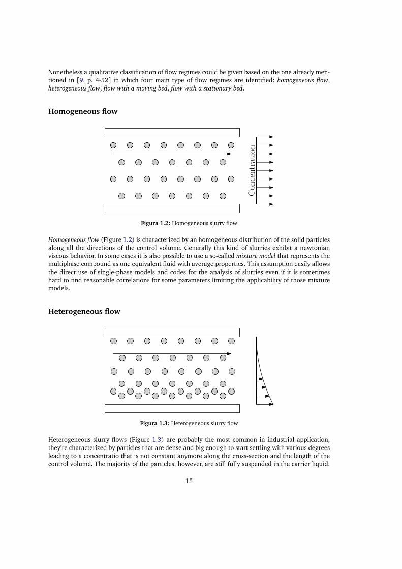
Nonetheless a qualitative classification of flow regimes could be given based on the one already men-tioned in [9, p. 4-52] in which four main type of flow regimes are identified: homogeneous flow,heterogeneous flow, flow with a moving bed, flow with a stationary bed.
Homogeneous flow
Concentration
Figura 1.2: Homogeneous slurry flow
Homogeneous flow (Figure 1.2) is characterized by an homogeneous distribution of the solid particlesalong all the directions of the control volume. Generally this kind of slurries exhibit a newtonianviscous behavior. In some cases it is also possible to use a so-called mixture model that represents themultiphase compound as one equivalent fluid with average properties. This assumption easily allowsthe direct use of single-phase models and codes for the analysis of slurries even if it is sometimeshard to find reasonable correlations for some parameters limiting the applicability of those mixturemodels.
Heterogeneous flow
Figura 1.3: Heterogeneous slurry flow
Heterogeneous slurry flows (Figure 1.3) are probably the most common in industrial application,they’re characterized by particles that are dense and big enough to start settling with various degreesleading to a concentratio that is not constant anymore along the cross-section and the length of thecontrol volume. The majority of the particles, however, are still fully suspended in the carrier liquid.
15

The analysis of this kind of regime cannot exempt from a model that keep intact the different pro-perties of the phases that have to be considered separately.
Moving bed flow
Figura 1.4: Moving Bed slurry flow
Moving Bed slurry flows (Figure 1.4) are observed when the larger and/or denser settling particleswill accumulate on the bottom of the volume forming a bed and reaching the maximum packing limit.In the bed zone of the volume frictional stresses are high enough to make the particles move or slidealong the length. The upper part of the volume, instead, is generally occupied by an heterogeneousslurry flow.
Stationary bed flow
Figura 1.5: Stationary Bed slurry flow
Stationary bed slurry flows (Figure 1.5) are encountered when the velocity of the slurry is not hi-gh enough to carry all the particles that form a stationary bed at the bottom. This kind of regime,as suggested in [9, p. 4-53] has to be avoided since it gives unstable flow or, in the worst cases,plugging.
16

1.1.1 Stokes number
A more quantitative attempt to establish the flow regime is the definition of the Stokes number St,its definition and physical meaning can be derived considering the equation of motion for a singlespherical particle in a fluid:
mdup
dt=
12
CD
πd2p
4ρc
u− up
u− up
(1.1)
considering the Stokes result for the drag coefficient of a sphere for Re→ 0:
CD =24Re
(1.2)
and the definition of a Reynolds number for the particle:
Rep =ρc D
u− up
µc=ρc D |ur |µc
(1.3)
the Equation (1.1) becomes:
dup
dt=
18µc
ρpd2p
u− up
=1τu
u− up
where the volume of a spherical particle has been considered for the mass
m= ρpV = 43ρpπ
d3p
8
.
This way a characteristic response time of a particle associated to momentum exchange between theparticle itself and the carrier fluid has been defined:
τu =18µc
ρpd2p
(1.4)
The Stokes number is defined as the ratio between the characteristic time of a particle τu and thecharacteristic time of the flow τ f :
St =τu
τ f=
18µc
ρpd2p
UD
(1.5)
17


Capitolo 2
State of the Art
In this chapter a literature survey about production, experimentation and modeling for cryogenictwo-phase flows is provided. The interest will be mainly focused on SLH2 as it is one of the majorcandidates for the use in the new generation space launchers or space planes like the NASP or theconcepts published in the frame of the ESA’s FESTIP but the concepts are in general extendable to allthe kind of slush flows used in several industrial and research applications like SLO2, Slush Nitrogen(SLN2) or Slurry Ice (SLH2O). A quite comprehensive research on literature about SLH2 is reportedin [10] while another review on production and utilization of SLH2 is in [11]; the main findings inthose papers are reported in this chapter with enrichments from other sources where needed.
2.1 Production Techniques
In the examined literature mainly two production techniques emerge: Auger method (Section 2.1.1)and Freeze-thaw method (Section 2.1.2) . Other methods are reported [10], [12] like Helium injectionor Magnetic Refrigeration but there is not comparable documentation and they will not be describedin this section.
2.1.1 Auger method
This metod is an alternative method to the one described in Section 2.1.2 that exploits the rotatingmovement of an auger that scrapes the solid layer of the fluid that froze on the cooled walls (sincelower temperatures than hydrogen Triple-point (TP) are needed, gaseous or liquid helium are chosenas refrigerant). Differently from the method described in Section 2.1.2 the process is completelycontinous and not alternate. The process has been reported for the production of SLH2 [13]–[15] butalso for SLO2 [15] and SLN2 [14], [16]. Problem with the auger locking, probably due to overcooling,is reported in [14]. In [15] the auger is also immersed in the liquid to be frozen. An image of a patent[17] describing a system for producing SLH2 with this method is showed in Figure 2.1.In [15] the auger method for producing SLH2 is described in details. It’s reported that, in spite of someirreversibilities associated to the extraction of the heat produced by the auger rotation, the systemsseems to require less energy then the Freeze-thaw (F-T) method. A relation also for the power needed
19

Figura 2.1: Image of auger method apparatus for producing SLH2 [17]
to produce slush with the auger method is suggested in Equation (2.1).Size of particles reported is: 0.1− 4 mm [15]
Pd = 0.0359ω+ 0.0014Pr For SLH2
Pd = 0.0359ω+ 0.0039Pr For SLO2(2.1)
where ω is the rotational speed of the auger, Pd total power required to rotate the auger, Pr therefrigeration supplied to the auger assembly [W].
2.1.2 Freeze-thaw method
A method to produce SLH2 that exploits periodic vacuum pumping of the ullage over the LH2 crea-ting solid layers on the surface. The pressure is lowered until the triple point of the LH2 (13.8K), asolid layer is hence produced. Following the production of the solid layer the pressure is allowed toincrease and the solid layer just produced melts near the vessel walls and sinks into the liquid henceforming slush ([1], [13], [18]–[20]). A patent regarding this production methodology is showed inFigure 2.2.
20

Figura 2.2: Image of freeze-thaw method for producing SLH2 [1]
An optimal rate of vacuum pumping is reported in [1] (0.91m3s−1 per m2of surface area for vacuumpump inlet conditions of 300K and 6.9kN m−2) and in [18] a relation among the parameters influen-cing the production time is given by Equation (2.2). Other example of this production technique forslush nitrogen are reported in [21].
t t
tmin= f
Ω0.5D0.75b D1.5
g t0.5th L
h0.5 V t f r
(2.2)
The particle size reported in [15] for previous F-T methods measurements are in the range of 0.5−10mm with 2 mm being the mosto common size.
2.2 Experimental Setups
2.2.1 Density Measurements
Gamma Radiation attenuation
γ-rays attenuation method is proposed as density measurement techniques in [1], [22]. The measu-rement principle is based on the Lambert’s Equation (Equation (2.3)):
21

I = I0e−µMρ l (2.3)
where I0 and I are the ingoing and outgoing γ-ray flux, ρ is the density of the sample, l the lenghtof the sample and µM the mass absorption coefficient. The µM coefficient is retrieved from XCOMdatabase [23]. In [22] is reported that relative error on density is function of µM, l, and ρ itselfEquation (2.4)
∆ρ
ρ=∆ll+
c′p
I0
(2.4)
being:
c′ =1−p
e−µMρ l
−µMρ lp
e−µMρ l
Statistical error are reported for density measurements on different type of slushes and in particularfor SLN2 an error of about 5.8% is highlighted.
Hydrostatic weighting
Capacitance and Waveguide Type
In [19], [24] densimeters based on capacitance changes are described. This kind of densimeter ex-ploits the difference between the specific dielectric constant during the shift from liquid (εl = 1.252)to solid (εs = 1.286)to estimate SLH2 density. The dielectric constant - density relation is provided bythe Clausius-Mossotti equation Equation (2.5) and the relation between capacitance and dielectricconstant is given in Equation (2.6):
ε − 1ε + 2
= ρP (2.5)
C = C0ε+ Cd (2.6)
When microwaves are transmitted through a medium whose dielectric constant is changing phaseshift ∆φ occurs. The phase shift is related to the dielectric constant change as showed in Equa-tion (2.7):
∆ε =λpε
180L∆φ (2.7)
beingλ the microwave wavelength, L the distance between receiving and transmitting antennas, ε thespecific dielectric constant. Accuracy within ±0.5% is reported for the density measurement.
22

Figura 2.3: Working principle of the capacitance/waveguide flowmeter [19], [24]
2.2.2 Flow rate measurements
Capacitance and Waveguide Type
Using two waveguide type densimeters described in Section 2.2.1 installed in two different locationsalong the piped flow the flow velocity is calculated from the densimeters distance and the delay timewhen the cross-correlation functions of the two density signals was at maximum (see Figure 2.3)being V the velocity measured, L the distance of the densimeters and τ the delay time of the cross-correlation peak detection instant.
When using microwaves the variation in the said constant influences the cutoff frequency fc by whichthe gain corresponding to the microwave transmission signal passing through the waveguide falls offlike a step function as highlighted by the equation Equation (2.8):
fc =c
3.41apε
(2.8)
The accuracy of the flowmeters is estimated to be «high enough» compared to the data achievedmeasuring the liquid level loss (±5%) but more experiments to confirm it are suggested.
2.2.3 Heat Transfer Measurements
Experiments and report on the heat transfer characteristics for SLH2 are somehow lacking in theliterature; [2], [20] describe similar approaches to the study of the nucleate boiling heat transferproperties of triple point SLH2, triple point LH2 and even SLN2 and LN2: a circular flat plate ofstainless steel of 0.025 m in diameter was used as the heat transfer surface for [2] while [20] uses anelectrolytic tough pitch copper circular flat plate of the same size. The effect of the orientation angleφ of the heat transfer surface is also investigated.
The experimental setups described in [20] consists of three glass Dewar vessels nested together filledrespectively, from the outer to the inner, of LN2, LH2 and SLH2. The purpose of the two most outervessels is to lower the heat leak into the SLH2 from the outer environment. The experimental setupis showed in Figure 2.4.
The major outcomes of the experiments are:
23
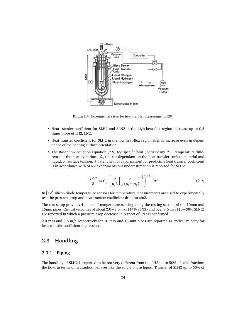
Figura 2.4: Experimental setup for heat transfer measurements [20]
• Heat transfer coefficient for SLH2 and SLN2 in the high-heat-flux region decrease up to 0.5times those of LH2, LN2.
• Heat transfer coefficient for SLH2 in the low-heat-flux region slightly increase even in depen-dance of the heating surface orientation
• The Rosenhow equation Equation (2.9) (cl : specific heat, µl : viscosity, ∆T : temperature diffe-rence at the heating surface, Cs f : factor dependant on the heat transfer surface material andliquid, σ: surface tension, λ: latent heat of vaporization) for predicting heat transfer coefficientis in accordance with SLN2 experiments but underestimation is reported for SLH2.
cl∆Tλ= Cs f
¨
qµlλ
σ
g (ρl −ρv)
12
«0.33
Prsl (2.9)
In [12] silicon diode temperature sensors for temperature measurements are used to experimentallytest the pressure drop and heat transfer coefficient drop for sln2.
The test setup provides 4 points of temperature sensing along the testing section of the 10mm and15mm pipes. Critical velocities of about 2.0−3.0 m/s (14% SLN2) and over 3.6 m/s (10−30% SLN2)are reported in which a pressure drop decrease in respect of LN2 is confirmed.
2.0 m/s and 3.6 m/s respectively for 10 mm and 15 mm pipes are reported as critical velocity forheat transfer coefficient depression.
2.3 Handling
2.3.1 Piping
The handling of SLH2 is reported to be not very different from the LH2 up to 50% of solid fraction:the flow, in terms of hydraulics, behaves like the single-phase liquid. Transfer of SLH2 up to 60% of
24

solid fraction is reported inside of 16.6 mm up to 25 mm diameter pipes [1]. The minimum velocitythat allows an homogeneous flow is reported to be 0.46 m/s for 16.6 mm diameter pipes.
In [25] a pipe of 15 mm is reported to be used for the grid and in [12], [26] pipes of 10 mm and 15mm are used.
2.3.2 Heat leaks and pressure oscillations
Pressure oscillations are reported to arise [1], [10], [27] caused by thermal leak in SLH2. Basicallythe flow encounters a warmer environment and starts to vaporize; the pressure increases pushing itback to the source, even repeatedly. And in [1] a precooling of the pipes before letting the SLH2 flowin them is strongly advised.
2.3.3 Pressurization
The triple point conditions for SLH2 (0.08 bar at 13.8K), in particular the low pressure, could leadto higly dangerous security issues since air could leak into the tank and forming an easily-explosivemixture with the hydrogen itself. Moreover the low pressure inside the tanks could also cause struc-tural problems (buckling). To overcome all this side effects pressurization with helium is reported in[1], [12], [13], [19], [24].
2.3.4 Aging
In [1] aging effects up to 100 hours are discussed. The aging phenomenon leads to an increase insettled slush density and in that paper it is explained as a result of heat leak into the slush. From asolid fraction of about 35− 45% for the freshly prepared slush after respectively 50 hours in a wellinsulated and shielded vessel (Q = 6.7 · 10−8 W
cm3 ) and 17 hours in a vacuum insulated glass vesselwith 20 times of heat imput a solid fraction of 60% is reached.
25


Capitolo 3
Numerical Modeling
Numerical simulation and Computational Fluid Dynamics (CFD) are tools that are gaining importancenowadays thanks to the quick increase of computational power density of modern, also commercial,processors. Often for multiphase flows, experimental sampling of some properties (i.e. velocity pro-files and phase fractions) are very hard to accomplish also because of the operating conditions (i.e.low temperatures and pressures). In this frame of perspectives the possibility to predict complex fieldsthanks to the use of numerical analysis is very important for an efficient development of technologicalresearch.
In this chapter an overview of the mathematical models available for the simulation of slush andmore generally slurry flows is discussed, with particular interest towards the Two-fluids model (2FM).Differences with the Lagrangian approach are briefly discussed and the Kinetic Theory for granularflows (KTGF) is also introduced.
3.1 Eulerian Two-Fluid Model
The considerations made in this section are focused to a system composed by two phases, a carrierliquid and a phase representing dispersed solid particles, but the Eulerian approach to multiphasemodeling can be (and actually it is) extended also to systems that are characterized by several morephases that could behave as solids, liquids or gases.
In the Eulerian approach both the carrier phase and the particulate are modeled as interpenetratingcontinua characterized by Eulerian fields (like velocity u (x, t)) that are described by averaged con-servation equations. The averaging process introduces the phase fraction αϕ which is defined as theprobability that a certain phase is present at a certain point in space and time. Applying the Principleof Conservation of Difficulty1 it is possible to understand how, even if several different regimes arepossible to be simulated with the Eulerian approach, the difficulty migrates to the additional term thatarises in the momentum conservation equation due to loss of information caused by the averagingprocess, named interphase momentum exchange term.
1Origin of this principle is somehow unknown. The author came into knowledge of it the first time when reported by Prof.Quartapelle in one of his Fluid Dynamics classes at Politecnico di Milano.
27
This chapter is dedicated to the formalization of the theoretical and numerical background of thework, a brief comparison against the Lagrangian approach is given in Section 3.1.1, comments aboutthe averaging process are reported in Section 3.1.2 with particular focus on physical differencesamong time, volume and ensemble averaging, the governing equations are described in Section 3.1.4and an overview on the KTGF that is used to model solid-fluid interactions is provided in Sec-tion 3.2.
Literature examples of use of this model on slush are not a lot, in [25], [28] an Finite Volume Method(FVM) Euler-Euler (E-E) approach is used to numerically model the problem. In [25] the choiceis justified in order to minimize the computational cost. Other examples of numerical simulationperformed in the frame of the Eulerian two-fluid model applied to slush flows are also [21], [29],[30]. In [31]–[33] the same theoretical and numerical background is applied to more classical slurrieslike sand-water, coal-water, glass-beads-water and ice slurry.
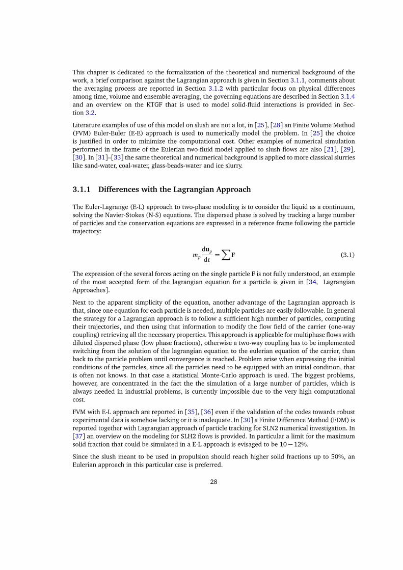
3.1.1 Differences with the Lagrangian Approach
The Euler-Lagrange (E-L) approach to two-phase modeling is to consider the liquid as a continuum,solving the Navier-Stokes (N-S) equations. The dispersed phase is solved by tracking a large numberof particles and the conservation equations are expressed in a reference frame following the particletrajectory:
mp
dup
dt=∑
F (3.1)
The expression of the several forces acting on the single particle F is not fully understood, an exampleof the most accepted form of the lagrangian equation for a particle is given in [34, LagrangianApproaches].
Next to the apparent simplicity of the equation, another advantage of the Lagrangian approach isthat, since one equation for each particle is needed, multiple particles are easily followable. In generalthe strategy for a Lagrangian approach is to follow a sufficient high number of particles, computingtheir trajectories, and then using that information to modify the flow field of the carrier (one-waycoupling) retrieving all the necessary properties. This approach is applicable for multiphase flows withdiluted dispersed phase (low phase fractions), otherwise a two-way coupling has to be implementedswitching from the solution of the lagrangian equation to the eulerian equation of the carrier, thanback to the particle problem until convergence is reached. Problem arise when expressing the initialconditions of the particles, since all the particles need to be equipped with an initial condition, thatis often not knows. In that case a statistical Monte-Carlo approach is used. The biggest problems,however, are concentrated in the fact the the simulation of a large number of particles, which isalways needed in industrial problems, is currently impossible due to the very high computationalcost.
FVM with E-L approach are reported in [35], [36] even if the validation of the codes towards robustexperimental data is somehow lacking or it is inadequate. In [30] a Finite Difference Method (FDM) isreported together with Lagrangian approach of particle tracking for SLN2 numerical investigation. In[37] an overview on the modeling for SLH2 flows is provided. In particular a limit for the maximumsolid fraction that could be simulated in a E-L approach is evisaged to be 10− 12%.
Since the slush meant to be used in propulsion should reach higher solid fractions up to 50%, anEulerian approach in this particular case is preferred.
28
3.1.2 Averaging
The classical turbulence treatment is based on the averaging of the N-S equations using a time-averageoperator and the so-called «Reynolds decomposition» that represents a general fluctuating propertyas:
u (x, t) = u (x) + u′ (x, t) (3.2)
where the first member in the Right Hand Side (RHS) represents a time averaged field,
u (x) = limT→∞
1T
∫ T
0
u (x, t)dt (3.3)
and the last expression in the RHS is the fluctuating part of the field.
An alternative classical approach to the averaging process of the N-S equations is the volume avera-ging,
u (x, t) = limV→δV
1V
∫
V
u (x, t)dV (3.4)
Both those approaches underlie constraints on the time/length scale that must be observed to keepthe meaning of the resulting equations (i.e. when they are applied to multiphase flows care must betaken to account properly time/length scales of particles and turbulence) [34, p. 41].
In [34, p. 42] the ensemble averaging is reported to be the most mathematically rigorous since itallows to consider time and length scales that could be also infinitesimal and a wide explanation alsoon the number of averaging steps to accomplish is given. The final directives of that discussion are touse the ensemble average as the only averaging operator to be applied to the equations. In this frameof work, the phase fraction α has to be considered as the probability that a certain phase is presentat a certain point in time and space.
Following the procedure reported in [34] and also employed in [38] , based on the work of [39],the conservation equations are derived conditioning the starting instantaneous microscopic equationswith a phase indicator function so that contributions to the averaged conservation equations come onlyfrom regions (in space and time) that contain that particular phase. The phase indicator function isdefined as
χϕ =
¨
1, If phase ϕ is present
0, Otherwise(3.5)
3.1.3 Turbulence Modeling
The turbulence modeling of two-phase systems is a complex topic and the closure equations may varyin dependence with the specific problem (i.e. bubble flow, solid-liquid, liquid-gas, etc...).
Generally the fundamental assumption that is made for the closure of the momentum equation is tomodel the Reynolds stress using the so-called Boussinesq hypothesis
29

µt = ρCµk2
ε(3.6)
the Reynolds stress are computed as expressed in Equation (3.24) here below reported for conve-nience,
R= −ρu′u′ = µt
∇u+∇uT −23ρkI (3.7)
while the turbulent kinetic energy and the turbulent dissipation rate behavior is described by twotransport equations:
∂ ραε
∂ t+∇ · (ραεu) =∇ ·
α
µ+µt
σε
∇ε
+ C1ραGε
k− C2ρα
ε
k+ραΠε (3.8)
∂ ραk∂ t
+∇ · (ραku) =∇ ·
α
µ+µt
σk
∇k
+ραG −ραε+ραΠk (3.9)
where in general Cµ = 0.09, C1 = 1.44, C2 = 1.92, σk = 1, σε = 1.3 and G is given by Equa-tion (3.10).
G = µt
∇u+∇uT (3.10)
The source terms Πk, Πε can be expressed in rapport to the specific problem, for example addres-sing for bubble-generated or particle-generated turbulence. More details on multiphase turbulencemodeling can be more deeply investigated reading [40].
3.1.4 Governing Equations
Mass Conservation
An example of the application of the conditioning process briefly described in Section 3.1.2 is he-re applied to the mass conservation equation (from [34]). Starting from the local mass balanceequation
∂ ρ
∂ t+∇ · (ρu) = 0 (3.11)
phase conditioning is applied ad then the ensemble averaging is performed resulting in
χϕ∂ ρ
∂ t+χϕ∇ · (ρu) = 0 (3.12)
that can be rearranged to give
30

∂ χϕρ
∂ t+∇ ·
χϕρu
= ρ∂ χϕ
∂ t+ρu · ∇χϕ (3.13)
The derivative of the phase indicator can be linked to the motion of the interface between phases[34, Appendix A]
∂ χϕ
∂ t= −vi · ∇χϕ (3.14)
so the equation becomes
∂ χϕρ
∂ t+∇ ·
χϕρu
= ρ (u− vi) · ∇χϕ (3.15)
The conditional averaged quantities (i.e. the quantities related to one specific phase ϕ are expressedas
γϕ =χϕγ
αϕ(3.16)
being γ a generic property (e.g. density ρ) and αϕ the phase fraction. This allows to write theEquation (3.15) as
∂ αϕρϕ
∂ t+∇ ·
αϕρϕuϕ
=
ρϕ
uϕ − vi
· n
i Σ (3.17)
where the notation ⟨γ⟩Σ is defined as the surface integral per unit volume divided by the surfacearea per unit volume Σ [34, Appendix A],
⟨γ⟩=1Σ
limδV→0
1δV
∫
δS
γdS (3.18)
where
Σ= limδV→0
1δV
∫
δS
dS (3.19)
This can be interpreted as the surface-weighted value of γ at the interface.
The last term of the RHS of Equation (3.17) is null for non-reacting interfaces (since the velocity ofthe interface vi is equal to the velocity of the phase ϕ at the interface). Hence the equation can besimplified as:
∂ αϕρϕ
∂ t+∇ ·
αϕρϕuϕ
= 0 (3.20)
31

Momentum conservation
Applying the same concepts of phase-conditioning and ensemble averaging an averaged version ofthe momentum conservation can be derived:
∂ αϕρϕuϕ∂ t
+∇ ·
αϕρϕuϕuϕ
+∇ ·
αϕReffϕ
= −αϕ∇p+αϕρϕg+Mϕ (3.21)
where Reffϕ is the combined turbulent and viscous stress
Reff= τ f +R (3.22)
being (with the hypothesis of incompressibility ∇ · u= 0)
τ f = µ
∇u+∇uT (3.23)
and
R= −ρu′u′ = µt
∇u+∇uT −23ρkI (3.24)
hence
Reff= (µ+µt)
∇u+∇uT −23ρkI (3.25)
and Mϕ is the interphase momentum exchange term.
3.1.5 Interphase Momentum Exchange
In the averaged momentum equation (Equation (3.21)) there is a term of each phaseϕ that embodiesthe exchange of momentum between them. It needs modeling.
First of all, since also the total momentum over all the phases is conserved, the sum of all theinterphase momentum exchange terms has to be zero
∑
ϕ
Mϕ = 0 (3.26)
Moreover, restricting the considerations on multiphase flows composed by two different phases, onlyone expression it is needed to close the system of equations. As reported in [38], the term is derivedconsidering all the forces acting on the single particle. The most important are: drag, lift, virtual mass,while other forces can be added as the Soret effect (also knows as termophoresis for liquid mixtures,i.e. the generation of a force caused by a strong temperature gradient, it is the symmetric effect ofthe Dufour effect) or turbulent dispersion (i.e. generation of a drag-like term due to turbulence andequation averaging).
32
Standard Phase Inversion
Mdraga αa
34ρbda
CD |ur |ur αaαb34
faCDaρb
db+ fb
CDbρa
da
|ur |ur
Mlifta αaCLρbur × (∇× ub) αaαb fa
CLaρbur × (∇× ua)
+αaαb fb
CLbρaur × (∇× ub)
Mv.m.a αaCv.m.ρb
DbubDt −
DauaDt
αaαb
faCv.m.aρb + fbCv.m.bρa
DbubDt
DauaDt
a, b are two generical phases. b is the continuous phase. da is the diameter of the dispersed phase. fa and fb are blendingfunctions such that αϕ → 0, fϕ → 0
DϕφDt =
∂ φ∂ t + uϕ · ∇
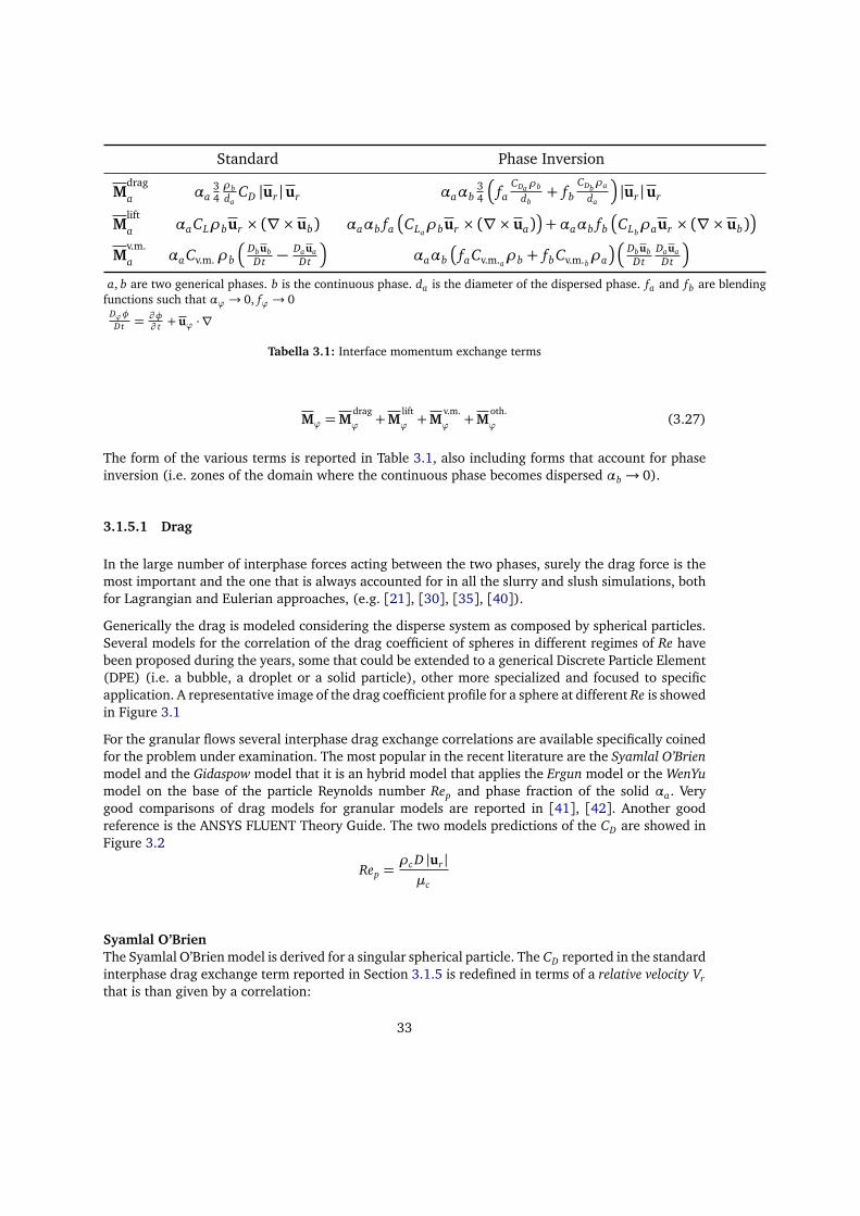
Tabella 3.1: Interface momentum exchange terms
Mϕ =Mdragϕ +M
liftϕ +M
v.m.ϕ +M
oth.ϕ (3.27)
The form of the various terms is reported in Table 3.1, also including forms that account for phaseinversion (i.e. zones of the domain where the continuous phase becomes dispersed αb → 0).
3.1.5.1 Drag
In the large number of interphase forces acting between the two phases, surely the drag force is themost important and the one that is always accounted for in all the slurry and slush simulations, bothfor Lagrangian and Eulerian approaches, (e.g. [21], [30], [35], [40]).
Generically the drag is modeled considering the disperse system as composed by spherical particles.Several models for the correlation of the drag coefficient of spheres in different regimes of Re havebeen proposed during the years, some that could be extended to a generical Discrete Particle Element(DPE) (i.e. a bubble, a droplet or a solid particle), other more specialized and focused to specificapplication. A representative image of the drag coefficient profile for a sphere at different Re is showedin Figure 3.1
For the granular flows several interphase drag exchange correlations are available specifically coinedfor the problem under examination. The most popular in the recent literature are the Syamlal O’Brienmodel and the Gidaspow model that it is an hybrid model that applies the Ergun model or the WenYumodel on the base of the particle Reynolds number Rep and phase fraction of the solid αa. Verygood comparisons of drag models for granular models are reported in [41], [42]. Another goodreference is the ANSYS FLUENT Theory Guide. The two models predictions of the CD are showed inFigure 3.2
Rep =ρc D |ur |µc
Syamlal O’BrienThe Syamlal O’Brien model is derived for a singular spherical particle. The CD reported in the standardinterphase drag exchange term reported in Section 3.1.5 is redefined in terms of a relative velocity Vrthat is than given by a correlation:
33

10-3 10-2 10-1 100 101 102 103 104 105 106
Reynolds Number
100
101
102
103
Sphere Drag Coefficient
Figura 3.1: Sphere drag coefficient at different regimes
34

CD = fCD(1−αa)
V 2r
(3.28)
fCD =
0.63+ 4.8
√
√
√Vr
Rep
!
(3.29)
Vr =12
A− 0.06Rep
+r
0.06Rep
2+ 0.12Rep (2B − A) + A2 (3.30)
A= (1−αa)4.14 (3.31)
B =
¨
0.8 (1−αa)1.28 if αa ≥ 0.15
(1−αa)1.28 if αa < 0.15
(3.32)
GidaspowThe Gidaspow model applies the Ergun model for higher solid fractions and the WenYu model other-wise:
CD =
¨
fCD (1−αa)−1.65 if αa ≤ 0.2
200αaµb(1−αa)daρb |ur |
+ 73 if αa > 0.2
(3.33)
the expression for the CD in case of αa > 0.2 is derived from the original expression that is written interms of the interphase exchange term:
Mdraga = 150
α2aµb
(1−αa) d2a
+αa74ρb
da|ur | (3.34)
The drag coefficient is given by:
fCD =
¨
24Rep(1−αa)
1+ 0.15
(1−αa)Rep
0.687
if (1−αa)Rep < 1000
0.44 if (1−αa)Rep ≥ 1000(3.35)
3.2 Kinetic Theory for granular flows
The Kinetic Theory for granular flows is a theory that extends the ideas and tools applied successfullyfor the kinetic theory of gases to flows characterized by dispersed particles. The dispersed particlesare treated statistically, characterized by a frequency distribution of velocities and collisions, and thefluctuating velocities are then related to the shear gradient. The final outcome of the application ofthis model to the granular flow is a transport equation that describes the behaviour of a «granulartemperature» Θ associated to the random movement of particles whose diffusion coefficients aregiven by (several different) empirical correlations.
The model implemented in Open source Field Operation And Manipulation (OpenFOAM) is derivedfrom [41], a wide description of the theoretical background and applications of the KTGF is presentin [43]. The notation in this section will follow the one proposed by [43].
35

0.0 0.1 0.2 0.3 0.4 0.5 0.6
Solid Volume Fraction
0
50
100
150
Dra
g C
oeffic
ient
Syamlal O'Brien
Gidaspow
Figura 3.2: Comparison between drag models [41]
36

3.2.1 Governing Equations
The granular temperature is defined as a measure of the particle velocity fluctuations
Θ =13
c′
(3.36)
the ⟨γ⟩ operator is an averaging operator defined as
⟨γ⟩=
∫
γ f dc
n(3.37)
n=
∫
f dc (3.38)
being f the frequency distribution of velocities, that is a function of time, position and instantaneousvelocity
f = f (t,x,c) (3.39)
The granular temperature behaviour is described by the Equation (3.40)
32
∂
∂ t(αsρsΘs) +∇ · (αsρsusΘs)
=
(−PsI+τs) :∇us︸ ︷︷ ︸
Production due toshear stress
+ ∇ · (κΘ∇Θ)︸ ︷︷ ︸
Diffusion
− γΘ︸︷︷︸
Dissipation due toinelastic collisions
+ ΦΘ︸︷︷︸
Dissipation/Productiondue to the interaction
with the carrier
(3.40)
where Ps is the granular pressure and represent the normal forces acting on the solid phase due toparticle interactions. τs is the stress tensor of the solid phase, κΘ is the granular conductivity, γΘ andΦΘ are two terms that describe production and/or dissipation of granular energy. Expression for allthe terms can be derived [43]:
τs = αsµs
∇us +∇uTs −
23(∇ · us) I
+ (−Ps +λs∇ · us) I (3.41)
Ps = ρsαsΘ [1+ 2 (1+ e) g0αs] (3.42)
λs =43α2
sρsds g0 (1+ e)
√
√Θ
π(3.43)
γΘ = 12
1− e2 α2
sρs g0
dspπΘ
32 (3.44)
ΦΘ = β
3Θ−βds |ur |
2
4αsρspΘπ
(3.45)
37
where λs is the bulk viscosity of the solid phase, e is the restitution coefficient that represents thepercentage of momentum conserved after a collision between two particles, g0 is a radial distributionfunction. β is the coupling coefficient for drag force that can be obtained from the interface dragexchange term:
Mdraga = αa
34ρb
daCD |ur |ur = βur (3.46)
Expression for κΘ,µs, g0 are given by several authors and summarized in Table 3.2.
3.2.2 Frictional Stress
When the solid phase fraction is high in a particular zone of the domain, lots of contacts among par-ticles occurr and a frictional stress derives from them that must be accounted for in the mathematicalmodel. In this state the collisions among particles could not be considered instantaneous as previou-sly done in the kinetic theory and the frictional stress is accounted for adding a term in the granularpressure and in the granular viscosity:
Ps = Pkinetic + Pf (3.47)
µs = µkinetic +µ f (3.48)
A semi-empirical expression for the normal component of the frictional stress is given by [44]:
Pf = F r(αs −min (αs))
n
αs,max −αs
p (3.49)
where F r, n, p are empirical constants. The frictional shear viscosity is than expressed by the Coulomblaw:
µ f = Pf sinδ (3.50)
being δ the angle of internal friction of the particle.
Another approach is suggested in [45] where the frictional normal stress is provided using the Equa-tion (3.51) and the viscosity is then obtained by the Equation (3.52).
Pf = A(αs −min (αs))n (3.51)
µ f =Pf sinδ
αs
s
16
∂ us∂ x −
∂ vs∂ y
2+
∂ vs∂ y
2+
∂ us∂ x
2
+ 14
∂ us∂ y +
∂ vs∂ x
2(3.52)
38

Granular viscosity µs
Syamlal et al. 45α
2sρsds g0 (1+ e)
q
Θπ +
115
pΘπρsds g0
(1+e)( 32 e− 1
2 )32−
e2
α2s +
112αsdsρs
pπΘ
32−
e2
Gidaspow 45α
2sρsds g0 (1+ e)
q
Θπ +
115
pΘπρsds g0 (1+ e)α2
s +16
pΘπρsdsαs +
1096
pΘπ
ρsds(1+e)g0
Lun et al. 45α
2sρsds g0 (1+ e)
q
Θπ +
115
pΘπ
ρsds g0(1+e)( 32 e− 1
2 )α2s
32−
12 e
+ 16
pΘπ
ρsdsαs( 34 e+ 1
4 )32−
e2
+ 1096
pΘπ
ρsds
(1+e)( 32−
12 e)g0
Granular conductivity κΘ
Syamlal et al. 2α2sρsds g0 (1+ e)
q
Θπ +
98
pΘπ
ρsds g0( 12+
e2 )
2(2e−1)α2
s
( 4916−
3316 )
+ 1532
pΘπ
αsρsds
( 4916−
3316 e)
Gidaspow 2α2sρsds g0 (1+ e)
q
Θπ +
98
pΘπρsds g0
12 +
e2
α2s +
1516
pΘπαsρsds +
2564
pΘπ
ρsds(1+e)g0
Lun et al. 2α2sρsds g0 (1+ e)
q
Θπ +
98
pΘπ
ρsds g0( 12+
e2 )
2(2e−1)α2
s
( 4916−
3316 e) + 15
16
pΘπ
αsρsds
e2
2 +14 e+ 1
4
( 4916−
3316 e) + 25
64
pΘπ
ρsds
(1+e)( 4916−
3316 e)g0
Radial Function g0
Lun and Savage
1− αsαs, max
−2.65αs,max
Sinclair and Jackson
1−
αsαs, max
13
−1
Gidaspow 35
1−
αsαs, max
13
−1
Tabella 3.2: Kinetic Theory Correlations

3.2.3 Johnson and Jackson BCs
The solid phase does not behave as the classical liquid on the walls, that means the classical no-slipcondition that it is usually used on the walls for a liquid is not considered correct for a particulate.Instead, in [44] is proposed a different boundary condition on walls that allows non-zero velocitieson the boundary. The derivation is done considering the balance of the tangential force per unit areaexerted on the boundary by the particles and the corresponding stress within the particle assemblynear the boundary. The tangential force is assumed to be (Coulomb’s law of friction applied to thematerial sliding on the surface):
T f = N f tanδ (3.53)
where N f is the normal component of the frictional stress. The rate of transfer of momentum tounit area of the surface due to collisions is given by the collisional frequency of particles
p3Θ/s times
the average tangential momentum exchanged per collision
φρpVpuslip
and the number of particlesadjacent to the unit area of the surface 1/ac. s is the average distance of a particle surface from thewall boundary, uslip is the difference between the velocity of the particle and the velocity of the wall(us − uwall), ac is the average boundary area per particle, ρp and Vp are respectively the density and
the volume of the particle
that is assumed to be spherical Vp = 1/6πd3p
, φ is a specularity coefficientthat is dependant from the average roughness of the surface and its values range from 0 (perfectspecular collision) to 1 (perfect diffuse collisions). In other words φ is a measure of the amount inpercentage of tangential momentum lost in a collision with the wall. Both s and ac are functions ofthe solid phase fraction:
s = dp
αs, max
αs
13
− 1
(3.54)
ac = d2p
αs, max
αs
23
(3.55)
In this case the expression αs, max stands for the phase fraction at maximum packing condition that isgenerally taken to be 0.65.
Equating all the contributions projected along theuslip
|uslip| direction gives the first boundary condition
for the particles velocity at wall.
uslip ·
σkinetic +σ f
· n
uslip
+
p3φρpπ
pΘ
uslip
6αs,max
1−
αsαs,max
23
+ N f tanδ = 0 (3.56)
In Equation (3.56) the first element in the Left Hand Side (LHS) is the total stress component along theuslip direction, the second is the collisional contribution to momentum balance, the third is the frictio-nal force in the same direction. σkinetic+σ f is the total stress tensor defined in the compressive sense,made by a collitional and a frictional contribution as reported in the introduction of [44].
Making a similar balance over the control volume showed in Figure 3.3 for the total energy and the«true» energy (opposed to the «pseudo-thermal» energy associated to the fluctuations of particles –analogy to the kinetic theory of gases) Equation (3.57) and Equation (3.58) are obtained.
40

n
us
uwall
1
2
Figura 3.3: Control volume for the the energy flux BC [44]
− n · q|1 − us · (σ · n)|1 + n · q|2 + uwall · (σ · n)|2 = 0 (3.57)
− n · q|1 + n · q|2 +D − uslip · Sbf = 0 (3.58)
q = q + qPT is the total heat flux composed by the summation of a true thermal heat flux q and apseudo-thermal one qPT.D is the rate of dissipation of pseudo-thermal energy due to inelastic collisions of particles with theunit area of the boundary whose expression is given in Equation (3.60). The last term is the frictionalheating caused by particles sliding over the surface. Sb = σ · n = Sb
c + Sbf is the total force per unit
area arising from kinetic and frictional contribution. Subtracting the two equations, Equation (3.59)is obtained.
− n · qPT = D + uslip · Sbc (3.59)
Sbc is the force per unit area acting on the boundary due to collisions, and it is already derived in
the second term of the Equation (3.56). The only expression that is missing is for D, that is given bythe energy loss per particle collision with the wall (1− ew)ρpVp
32Θ, the collision frequency and the
number of particles adjacent to the unit area of the wall surface as already given before.
D =
14πρpd3
pΘ (1− ew)
p3Θ
dp
αs,max
αs
13 − 1
1
d2p
αs, max
αs
23
(3.60)
ew is the restitution coefficient of the wall, i.e. the amount of normal momentum lost hitting thewall.
In this section Equation (3.56) and Equation (3.59) have been described, those are the boundaryconditions to be applied respectively to the us and Θ fields in the comprehensive system of resolvingequations of the problem under examination.
3.3 Validation
A numerical model, to be useful for industrial application, must be validated on experimental dataand/or on other validated numerical results (e.g. Direct Navier-Stokes Simulation (DNS)). Experi-mental data for slush flows are not so common in literature and in addition, apart from the data
41

available about the pressure drops in pipe geometries, the sampling of the phase fractions and thesolid phase velocity is somehow problematic due to the intrinsic choking tendency of probes for thisking of flows and to the low temperatures needed for the production and use of those kind of flows.However in the documents collected by the author, the most promising techniques to sample consi-stently those properties is the Particle Image Velocimetry (PIV). In [25] the validation is carried onusing PIV together with experimental outcomes from [12], [26], meanwhile in [44] only the meanvalues are sampled. No profiles are given. The work in [1] is also showing mean parameters, noprofiles.
42

Capitolo 4
Correlations and EngineeringModels
Flows with dispersed particulate within a liquid carrier are of big importance in the industrial fra-mework. For this reason, next to more computational intensive toolset fast and reliable engineeringmodels are also needed to perform preliminary size and estimations.
For what concerns slush flows, empirical correlations and tools are very rare, the only example thatwas possible to find is a tool developed by NASA named FLow of slUSH (FLUSH) for sizing of pi-pelines of SLH2 in the frame of Shuttle program and later ones (e.g. NASP) briefly mentioned inSection 4.1.
Widening the point of view to general slurry flows, the situations improves and several correlationsand models are available in the literature, both purely empirical and mechanistic semi-empiricalattempts that show conflicting applicability in dependency to the various problem properties (e.g.solid-liquid density ratio, pipe diameter, ...).Nonetheless, assuming that a slush flow could be modeled as a slurry flow – and this might be con-sidered as an hazardous assumption since the shape of solid particles is not well determined in slushflows and it is still debatable that the behavior of a slush flow could be compared in analogy to slurryflows – when interested to the hydrodynamic behavior, that means neglecting the very important fea-ture of phase change, could be a first step towards the set up of a correlation or engineering modelfor slushes. A good overview on empirical correlations is reported in [46].
In this section a brief evaluation of some experimental correlation available to estimate pressure dropsand nature of the flow for slurries is performed and discussed. A lightweight Python library namedpyslurry is also introduced.
4.1 FLow of slUSH
At NASA a software tool named FLUSH was developed to calculate pressure drops and solid fractionlosses within different elements of a pipeline system of SLH2 solving one-dimensional steady-stateenergy equation Equation (4.1) and Bernoulli’s equation Equation (4.2) [47].
43

∆
h+|u|2
2+ gz
=Qm−Ws (4.1)
∆
pρ+|u|2
2+ gz
+Ws = 0 (4.2)
where Ws is the shaft work
Jkg =
m2
s2
The thermo-physical properties of the SLH2 are retrieved using GASPLUS, a FORTRAN 77 programdescribed in [48]. The software allows the user to specify several different elements of the pipelinelike elbows, valves and straight pipe segments, and is equipped with the capability of heat-leaksautomated calculation for vacuum-jacketed piping if not available.
The assumption made in the model which the program is based on are reported to be:
• Steady-state flow exists in the system
• Fluid is incompressible
• Lines are pre-cooled to TP
• Slush is well-mixed at the entrance of the line and settling effects are neglected
• The viscosity of the slush is equal to the LH2 (since the SLH2 viscosity is unknown)
• Heat of fusion is a constant
• Heat flux is used first (and only) to melt solids in a isotherm and constant pressure process
The algorithm pseudo-code described in [47] is reported in Algorithm 1.
4.2 Durand and Condolios
Durand and Condolios are one of the pioneers in the field of slurry flows. They carried out severalexperiments on sands and gravels whose results are explained in [49]. The original correlation iswritten in terms of relative head loss (Equation (4.3)), being islurry the head loss of the slurry, ipure thehead loss of the relative pure fluid (e.g. water), C the volumetric concentration of the solids.
islurry − ipure
ipureC=∆pslurry −∆ppure
∆ppureC= Φ (4.3)
In [46] a modification of the original correlation is reported, suggested by Gibert, to be as in Equa-tion (4.4).
Φ= Kψ−32 (4.4)
44

Algorithm 1 FLUSH algorithm for computation of SLH2 [47]1: Initialize temperatures, pressures, slush solid fraction, heat leak, element length, diameter and height2: while Yi > 0 and err (p, T )< tol do3: Use GASPLUS to obtain initial-element SLH2 properties4: ρl = ρl (Ti , pi)5: µl = µl (Ti , pi)6: Calculate an effective slush density at the inlet7: ρmix = Yiρs + (1− Yi)ρl8: Calculate mass flow rate and Reynolds number (using liquid viscosities)9: Calculate a friction factor using the Darcy-Weisbach correlation or National Institute of Standards and Technology
(NIST)’s slush correlations10: Calculate the downstream pressure from Bernoulli’s equation11: p f = pi +∆p12: Obtain final-element hydrogen properties from GASPLUS13: ρl = ρl
T f , p f
14: µl = µl
T f , p f
15: Obtain initial and final enthalpies from GASPLUS16: Hl, f = Hl, f
T f , p f
17: Hl,i = Hl,i (Ti , pi)18: Calculate initial mixture enthalpy19: Hmix,i = Hl,i − Yi Hfus20: Calculate final mixture enthalpy from energy equation21: Hmix, f = Hmix, i +∆H22: Calculate the change in slush solid fraction due to heat
23: Yf ,heat =Hl, f −Hmix, f
Hfus24: Calculate the change in slush solid fraction due to friction25: ∆Yfrict =
fHJ
fus26: Calculate the slush fraction at the element exit27: Yf = Yf ,heat −∆Yfrict28: end while
45

ψ= F r2fl F r−1
p (4.5)
F rp =1
p
Cx
=vt
Æ
gdp
(4.6)
F rfl =u
p
gDη(4.7)
η=ρp
ρl(4.8)
where g is the gravitational field, vt is the terminal settling velocity of the particles, dp the diameterof the particles, D the hydraulic diameter of the duct, ρp and ρl the densities of the particle and thecarrier liquid respectively, u the velocity of the slurry. The modification suggested by Gibert lies in thedefinition of the flow Froude number Ffl since in the original paper by Durand and Condolios [49]that number is defined without the density ratio η at the denominator.
4.2.1 Terminal Velocity correlations
The Durand and Condolios correlation reported in Equation (4.4) needs an estimation of the terminalvelocity of the particles vt , or equivalently, of the drag coefficient CD, since by the definition of theterminal velocity (informally «the terminal velocity is the velocity for which the gravitational forceequates the buoyancy and drag forces») the two parameters are related by Equation (4.9).
CD =43(η− 1) g
v2t
(4.9)
In the original paper few hints are given, often in terms of graphs relating the Froude numbers, whilein [46] the Zanke correlation for the terminal velocity is used (Equation (4.10)). Several correlationsare analyzed in [50] and another correlation, this time for the drag coefficient, is given by [51] andreported in Equation (4.11) and Equation (4.12) for convenience.
vt =10νl
dp
1+ 0.01(s− 1) gd3
ν2l
0.5
− 1
(4.10)
Λ= Rep
p
CD =
43
gd3pρl (ρs −ρl)
µl
(4.11)
log10
Rep
= −1.38+ 1.94 log10Λ− 8.60e−2 log2Λ− 2.52e−2 log3Λ
+ 9.19e−4 log4Λ+ 5.35e−4 log5Λ (4.12)
The prediction quality of the Durand-Condolios correlation together with the two Zanke and Turiandrag estimation are showed in Figure 4.1.The quality of prediction is not satisfying also considering that the cross-check data are collectedby the original work of Durand. The computation is performed using pyslurry library, a brief userguide is referred in Chapter A.
46

2.0 2.5 3.0 3.5 4.0 4.5 5.0
Velocity [m/s]
−5
0
5
10
15
20
25
30
35
40
Phi []
Durand-Condolios wrt Experimental Data
Zanke Drag Model
Turian Drag Model
L4-D0p15
(a) Durand-Condolios Estimation for L4 Sands
2.5 3.0 3.5 4.0 4.5
Velocity [m/s]
0
10
20
30
40
50
60
Phi []
Durand-Condolios wrt Experimental Data
Zanke Drag Model
Turian Drag Model
L8-D0p15
(b) Durand-Condolios Estimation for L8 Sands
Figura 4.1: Durand-Condolios correlation prediction on L4, L8 Sands
47

4.3 Turian and Yuan Correlations
Another example of correlations for slurry flows is given by Turian et al. in [51]. Differently fromwhat Durand et al. did, Turian and coworkers provide different correlations for different regime ofslurry flow, together with means to estimate the nature of flow on the basis of typical parameterscharacterizing a slurry. In that work, four different regimes are identified: flow with a stationary bed,saltation flow, heterogeneous flow, homogeneous flow, those regimes can be delineated computingsome regime numbers Ri j , when these regime numbers reach the value of 1, transition occurs. Thefunctional structure of this regime numbers is given by Equation (4.13).
Ri j =u2
k1Cn1 f n2w Cn3
D Dg(η− 1)(4.13)
where k1, n1, n2, n3 are empirical parameters given by the paper. fw is the Fanning friction factor of theassociated pure liquid. An example for the regime number associated to the transition from stationarybed (0) to saltation (1) is given in Equation (4.14).
R01 =u2
31.93C1.083 f 1.064w C−0.06160
D Dg(η− 1)(4.14)
Once the regime is identified, specific pressure-drop correlations can be applied. The pressure dropis given relatively to the friction factor of the associated pure fluid of the slurry (i.e. water) and thefunctional form of a pressure drop correlation is of the type:
f − fw = k1C n1 f n2w C n3
D
u2
Dg (η− 1)
n4
(4.15)
Also considering the higher flexibility of the correlations provided by Turian and coworkers, fromtests performed on several different dataset of slurries, the results are not satisfying. The regimedelineation often failed in the correct determination of the flow, hence predicting wrong pressuredrops. In addition to that, in a future work always by Turian et al. [52], the same correlations are cross-referenced, but they appear with a different prefactor, for example for stationary bed regime:
f − fw = 0.4936C0.7389 f 0.7717w C−0.4054
D
u2
Dg (η− 1)
−1.096
[51] (4.16)
f − fw = 12.127C0.7389 f 0.7717w C−0.4054
D
u2
Dg (η− 1)
−1.096
[52] (4.17)
(4.18)
That circumstance raises some doubts about the correctness of the formulas, also considering thatthe difference between the two prefactors are not constant among the different correlations leadingto some sort of ambiguity. Still, the model of Turian has been coded in pyslurry with the hope thatcommunity contributions could help to clarify the situation.
48

Capitolo 5
Results
Several different runs of simulations have been performed as benchmark of the model. Since notmany experimental data for slush flows are available in literature, together with configuration withSLN2, also cases run for a «more classical» water-glass-beads have been performed comparing theresults with the experimental data available on [53].
A sensitivity analysis on the Kaushal case has been performed to compare the effect of the va-rious parameters that can be tuned in the KTGF in addition to the effects of mesh and turbulencemodels.
5.1 Notes on Convergence
twoPhaseEulerFoam is a transient solver, it is not possible to set up a steady state as differently itis possible on FLUENT. To keep the two kind of simulations as similar as possible, the convergencecriterion has been established to stop the simulation when the pressure drop across the pipe reach asteady value. An example of a pressure drop profile over simulated time with a zoom over the lasttime iterations is reported in Figure 5.1. As it is possible to see, the pressure drop keeps oscillatingas if it was the response of an undamped marginally stable harmonic system, for this reason the finalvalue of the pressure drop reported in the next sections has been calculated as a mean value of thelast 400 time iterations.
For what concerns the numerical schemes, the twoPhaseEulerFoam solver in OpenFOAM is veryirritable, the mesh has to be very smooth and for the simulations performed in this work, the AspectRatio (AR) has not to exceed a value of ∼ 20 or the pressure calculations started to oscillate leadingvery often to divergence and crash. In order to account for this intrinsic sensitivity to the mesh,first-order schemes (upwind) have been chosen for all the fluxes ( divSchemes in OpenFOAM) toobtain as stability as possible. Another important parameter to monitor is the Courant Number Co,value too near to 1 led to instability and divergence in particular at the starting up. This is probablyalso addressable to the semi-implicit nature of the MUlti-dimensionsal Limiter for Explicit Solution(MULES) solver for the phase fraction equation used in OpenFOAM. As a probably too conservativerule in the following simulations the Co has been constrained to not be greater than 0.5.
49

0.0 0.5 1.0 1.5 2.0
Time [s]
−100000
−50000
0
50000
100000
150000
Pressure Drop [Pa]
Pressure Drop
1.95 1.9910700
10800
Figura 5.1: Pressure drop profile over time
50

Figura 5.2: Base mesh for all the cases
5.2 Initial and Boundary Conditions
The mesh for all the simulations, both for the Kaushal and slush case, is created using the blockMeshutility provided by OpenFOAM using a parametrizable cylinder.m4 or halfcylinder.m4 file thatis compiled using the GNU m4 macro preprocessor, allowing to change the geometrical dimensionsof the mesh and the number of cells per block easily. blockMesh creates structured mesh made ofhexahedral blocks. An example of the mesh is shown in Figure 5.2.
The mesh is composed respectively by 3 different patches (inlet, outlet and walls for the normalfull-size cylinder, by 4 instead for the half-cylinder (the fourth patch is the symmetry plane). BCs forall the fields must be set on all the patches and for the initial internal field. For the inlet patch,uniform constant profiles have been configured for all the fields. Also constant profiles are providedfor initialization of the internal field. On the walls, for the turbulent fields k,ε,ω,νt wall functionsare used since y+ > 30 averagely over all the domain. At the outlet the gradients of all the fields arefixed to zero (except for the pressure that has instead a fixed value since it is not possible to fix boththe pressure and the velocity on the same boundary - it would cause an over-constrained problem).The BCs are summarized in Table 5.1.
51
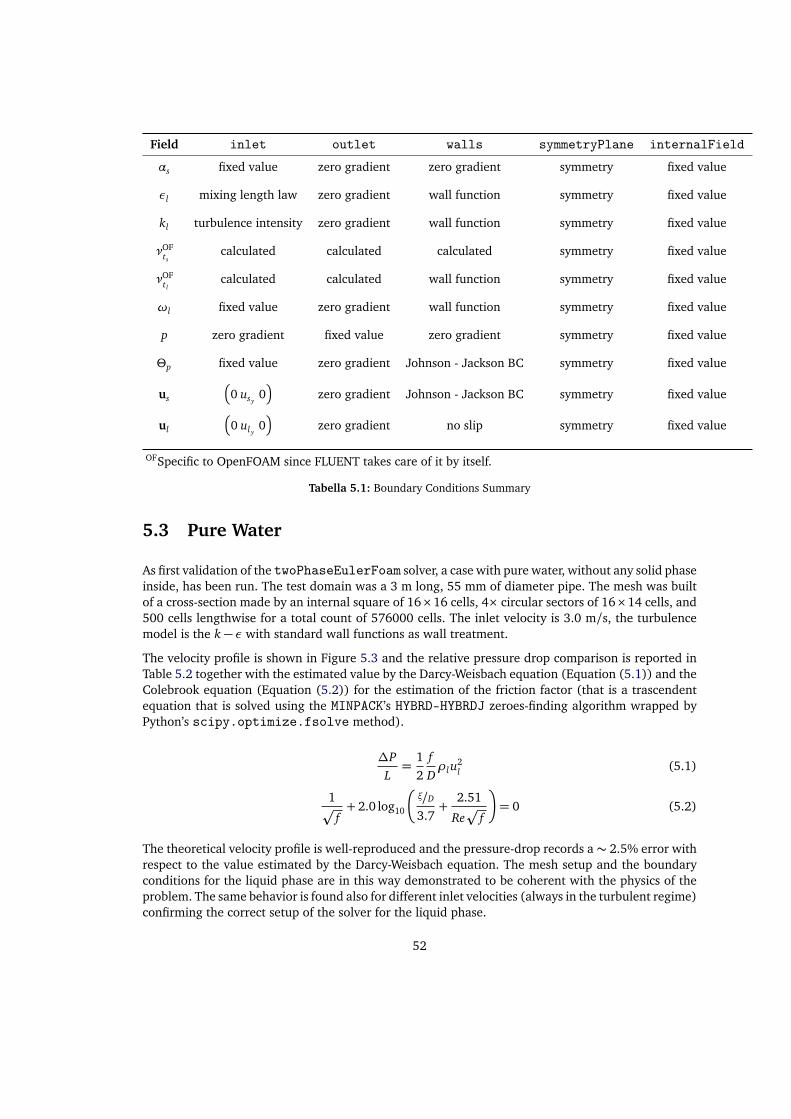
Field inlet outlet walls symmetryPlane internalField
αs fixed value zero gradient zero gradient symmetry fixed value
εl mixing length law zero gradient wall function symmetry fixed value
kl turbulence intensity zero gradient wall function symmetry fixed value
νOFts
calculated calculated calculated symmetry fixed value
νOFt l
calculated calculated wall function symmetry fixed value
ωl fixed value zero gradient wall function symmetry fixed value
p zero gradient fixed value zero gradient symmetry fixed value
Θp fixed value zero gradient Johnson - Jackson BC symmetry fixed value
us
0 usy0
zero gradient Johnson - Jackson BC symmetry fixed value
ul
0 ul y0
zero gradient no slip symmetry fixed value
OFSpecific to OpenFOAM since FLUENT takes care of it by itself.
Tabella 5.1: Boundary Conditions Summary
5.3 Pure Water
As first validation of the twoPhaseEulerFoam solver, a case with pure water, without any solid phaseinside, has been run. The test domain was a 3 m long, 55 mm of diameter pipe. The mesh was builtof a cross-section made by an internal square of 16×16 cells, 4× circular sectors of 16×14 cells, and500 cells lengthwise for a total count of 576000 cells. The inlet velocity is 3.0 m/s, the turbulencemodel is the k− ε with standard wall functions as wall treatment.
The velocity profile is shown in Figure 5.3 and the relative pressure drop comparison is reported inTable 5.2 together with the estimated value by the Darcy-Weisbach equation (Equation (5.1)) and theColebrook equation (Equation (5.2)) for the estimation of the friction factor (that is a trascendentequation that is solved using the MINPACK’s HYBRD-HYBRDJ zeroes-finding algorithm wrapped byPython’s scipy.optimize.fsolve method).
∆PL=
12
fDρlu
2l (5.1)
1p
f+ 2.0 log10
ξ/D
3.7+
2.51
Rep
f
= 0 (5.2)
The theoretical velocity profile is well-reproduced and the pressure-drop records a ∼ 2.5% error withrespect to the value estimated by the Darcy-Weisbach equation. The mesh setup and the boundaryconditions for the liquid phase are in this way demonstrated to be coherent with the physics of theproblem. The same behavior is found also for different inlet velocities (always in the turbulent regime)confirming the correct setup of the solver for the liquid phase.
52

0.0 0.1 0.2 0.3 0.4 0.5
r/D
0.0
0.2
0.4
0.6
0.8
1.0
U/m
ax(U
)
One seventh law
twoPhaseEulerFoam k-e
pimpleFoam k-e
Figura 5.3: Velocity profile for pure water
twoPhaseEulerFoam pimpleFoam Darcy-Weisbach
1361.2 1382.9 1330.5
Tabella 5.2: Pure water pressure drop
53

Pipe Diameter [mm] Liquid Viscosity [Pa s] Solid Density
kgm3
Liquid Density
kgm3
55 1e−3 2470 1000
Tabella 5.3: Kaushal case properties
5.4 Water-Glass-Beads slurry (Kaushal)
The first multiphase case simulated using OpenFOAM is a more classical, with respect to slush flows,slurry flow characterized by water as liquid carrier and glass-beads as solid particulate.The choice to perform an analysis of this kind has been driven by the fact that the shape of theparticles in this case is well-established to be spherical and also because more experimental dataare available in literature. In Table 5.3 the geometric and thermo-physical properties of the case arereported.
The benchmark case chosen is the one reported in [53]. First of all a sensitivity analysis over theseveral parameters that could be tuned in the KTGF is performed, the most important effects of pa-rameters variation are highlighted. Then a complete set of simulations is performed and is comparedwith experimental data from [53].
5.4.1 Sensitivity analysis for the KTGF
In the Section 3.2 the Kinetic Theory for granular flows is presented. From the details there describedis clear as there are several parameters that can be modified and that can influence the results of thesimulation. In the literature analyzed some suggestions are given about few parameters, in particularthe restitution coefficient e and the specularity coefficient φ, both for walls bouncing and internalcollisions, in [29] are taken with the values of, respectively, of ew = 0.99, e = 0.9, φ = 0.0001 whilein [21] φ = 0.02. Moreover a maximum packing limit for the phase fraction is given αmax = 0.52 forslush nitrogen. It’s clear as those parameters show a behaviour that is strongly case-specific, hence theneed for a sensitivity analysis over the several different tunable parameters and models has emerged.A summary of the different modifications done is summarized in Table 5.4 in terms of effects on thepressure drop along the pipe.
From the analysis of Table 5.4 is possible to understand how the most important parameter, in termsof influence over the pressure drop, is the specularity coefficient φ. This importance could be easilyunderstood since φ represents the amount in percentage of tangential momentum loss at the wall.As in a «normal» pure-liquid situation where the viscosity and the boundary layer that it is creatednear the wall influence the pressure loss, also here the wall interaction is very important even if thephysical process that creates the momentum loss is not fully related to friction, but also to collisionsof solid particles with the wall itself (see Section 3.2.3).
Pressure drop is not the only property of interest. Also the distribution of the solid phase along thediameter in a cross-section and the velocity profile are interesting. A selection of cases are comparedin terms of velocity profiles in Figure 5.4 and in terms of phase fraction dispersion over the diameterin Figure 5.5. Moreover a comparison between the Gidaspow and the Syamlal model is also shownin Figure 5.6 and Figure 5.7.
54

Case Name Particle Diameter [mm] Drag Model Viscosity Conductivity Granular Pressure Frictional Model Radial Model δ αmax e ew φ Y + ∆PL
Pam
gidasphi 44e−3 Gidaspow-Ergun-WenYu Gidaspow Gidaspow Lun Schaeffer SinclairJackson 30 0.64 0.9 0.9 0.01 37 2309gidasphi075 44e−3 Gidaspow-Ergun-WenYu Gidaspow Gidaspow Lun Schaeffer SinclairJackson 30 0.64 0.75 0.9 0.01 37 2249gidasphie 44e−3 Gidaspow-Ergun-WenYu Gidaspow Gidaspow Lun Schaeffer SinclairJackson 30 0.64 0.9 0.2 0.01 37 2309
gidasphie099 44e−3 Gidaspow-Ergun-WenYu Gidaspow Gidaspow Lun Schaeffer SinclairJackson 30 0.64 0.9 0.99 0.01 37 2309gidasphiam 44e−3 Gidaspow-Ergun-WenYu Gidaspow Gidaspow Lun Schaeffer SinclairJackson 30 0.5 0.9 0.9 0.01 37 4329
gidasphiam0001 44e−3 Gidaspow-Ergun-WenYu Gidaspow Gidaspow Lun Schaeffer SinclairJackson 30 0.5 0.9 0.9 0.001 37 1965gidasphi002 44e−3 Gidaspow-Ergun-WenYu Gidaspow Gidaspow Lun Schaeffer SinclairJackson 30 0.64 0.9 0.9 0.02 43 3354gidasphi005 44e−3 Gidaspow-Ergun-WenYu Gidaspow Gidaspow Lun Schaeffer SinclairJackson 30 0.64 0.9 0.9 0.05 43 7137gidasnofrict 44e−3 Gidaspow-Ergun-WenYu Gidaspow Gidaspow Lun Schaeffer SinclairJackson 0 0.64 0.9 0.9 0.01 36 2239gidasfr25 44e−3 Gidaspow-Ergun-WenYu Gidaspow Gidaspow Lun Schaeffer SinclairJackson 25 0.64 0.9 0.9 0.01 37 2255gidasphijj 44e−3 Gidaspow-Ergun-WenYu Gidaspow Gidaspow Lun JohnsonJackson SinclairJackson 28.5 0.64 0.9 0.9 0.01 37 2290
gidasphijj002 44e−3 Gidaspow-Ergun-WenYu Gidaspow Gidaspow Lun JohnsonJackson SinclairJackson 28.5 0.64 0.9 0.9 0.02 37 3122gidasphils 44e−3 Gidaspow-Ergun-WenYu Gidaspow Gidaspow Lun Schaeffer LunSavage 30 0.64 0.9 0.9 0.01 37 2229
gidasphismall 1.25e−4 Gidaspow-Ergun-WenYu Gidaspow Gidaspow Lun Schaeffer SinclairJackson 30 0.64 0.9 0.9 0.01 43 3650gidasphigibilaro 44e−3 Gibilaro Gidaspow Gidaspow Lun Schaeffer SinclairJackson 30 0.64 0.9 0.9 0.01 37 2478
syamlal 1.25e−4 Syamlal-OBrien Syamlal Syamlal Syamlal-Rogers-OBrien Schaeffer SinclairJackson 30 0.64 0.9 0.9 0.01 43 3580syamlaljj 1.25e−4 Syamlal-OBrien Syamlal Syamlal Syamlal-Rogers-OBrien JohnsonJackson SinclairJackson 28.5 0.64 0.9 0.9 0.01 43 3580
syamlaljj002 1.25e−4 Syamlal-OBrien Syamlal Syamlal Syamlal-Rogers-OBrien JohnsonJackson SinclairJackson 28.5 0.64 0.9 0.9 0.02 43 3880syamlaljj0001 1.25e−4 Syamlal-OBrien Syamlal Syamlal Syamlal-Rogers-OBrien JohnsonJackson SinclairJackson 28.5 0.64 0.9 0.9 0.001 43 3431
u= 3.0 ms ,α= 0.30,αmin f
= 0.5, Turbulence model: k− ε.In black the modifications with respect to the base case that is gidasphi.
Tabella 5.4: Sensitivity Analysis for Kaushal Case
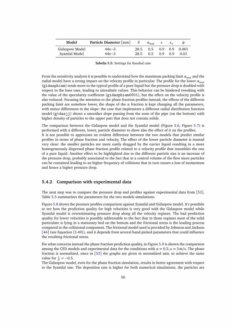
Model Particle Diameter [mm] δ αmax e ew φ
Gidaspow Model 44e−3 28.5 0.5 0.9 0.9 0.001Syamlal Model 44e−3 28.5 0.5 0.9 0.9 0.01
Tabella 5.5: Settings for Kaushal case
From the sensitivity analysis it is possible to understand how the maximum packing limit αmax and theradial model have a strong impact on the velocity profile in particular. The profile for the lower αmax(gidasphiam) tends more to the typical profile of a pure liquid but the pressure drop is doubled withrespect to the base case, leading to unrealistic values. This behavior can be hindered tweaking withthe value of the specularity coefficient (gidasphiam0001), but the effect on the velocity profile isalso reduced. Focusing the attention to the phase fraction profiles instead, the effects of the differentpacking limit are somehow lower, the shape of the α fraction is kept changing all the parameters,with minor differences in the slope: the case that implements a different radial distribution functionmodel (gidasjj) shows a smoother slope passing from the zone of the pipe (on the bottom) withhigher density of particles to the upper part that does not contain solids.
The comparison between the Gidaspow model and the Syamlal model (Figure 5.6, Figure 5.7) isperformed with a different, lower, particle diameter to show also the effect of it on the profiles.It is not possible to appreciate an evident difference between the two models that predict similarprofiles in terms of phase fraction and velocity. The effect of the lower particle diameter is insteadvery clear: the smaller particles are more easily dragged by the carrier liquid resulting in a morehomogeneously dispersed phase fraction profile related to a velocity profile that resembles the oneof a pure liquid. Another effect to be highlighted due to the different particle size is an increase ofthe pressure drop, probably associated to the fact that in a control volume of the flow more particlescan be contained leading to an higher frequency of collisions that in turn causes a loss of momentumand hence a higher pressure drop.
5.4.2 Comparison with experimental data
The next step was to compare the pressure drop and profiles against experimental data from [53].Table 5.5 summarizes the parameters for the two models simulations.
Figure 5.8 shows the pressure profiles comparison against Syamlal and Gidaspow model. It’s possibileto see how the prediction quality for high velocities is very good with the Gidaspow model whileSyamlal model is overestimating pressure drop along all the velocity regimes. The bad predictionquality for lower velocities is possibly addressable to the fact that in those regimes most of the solidparticulate is lying in a stationary bed on the bottom and the frictional stress is the leading processcompared to the collisional component. The frictional model used is provided by Johnson and Jackson[44] (see Equation (3.49)), and it depends from several hand-picked parameters that could influencethe resulting frictional stress.
For what concerns instead the phase fraction prediction quality, in Figure 5.9 is shown the comparisonamong the CFD models and experimental data for the conditions with α= 0.3, u= 3m/s. The phasefraction is normalized, since in [53] the graphs are given in normalized axis, to achieve the samevalue for r
D = −0.5.The Gidaspow model, even for the phase fraction simulation, results in better agreement with respectto the Syamlal one. The deposition rate is higher for both numerical simulations, the particles are
56

−0.4 −0.2 0.0 0.2 0.4
r/D
1.5
2.0
2.5
3.0
3.5
4.0
Velocity [m/s]
gidasphi
gidasphi002
gidasphiam
gidasphiam0001
gidasphijj
Figura 5.4: Velocity Profiles comparison for Gidaspow model
57

0.0 0.2 0.4 0.6 0.8 1.0
Phase fraction
−0.4
−0.2
0.0
0.2
0.4
r/D
gidasphi
gidasphi002
gidasphiam
gidasphiam0001
gidasphijj
Figura 5.5: α Profiles comparison for Gidaspow model
58

−0.4 −0.2 0.0 0.2 0.4
r/D
1.5
2.0
2.5
3.0
3.5
4.0
4.5
5.0
Velocity [m/s]
gidasphismall
syamlal
Figura 5.6: Gidaspow vs Syamlal velocity profiles comparison
59

0.0 0.2 0.4 0.6 0.8 1.0
Phase fraction
−0.4
−0.2
0.0
0.2
0.4
r/D
gidasphismall
syamlal
Figura 5.7: Gidaspow vs Syamlal α profiles comparison
60

2.0 2.5 3.0 3.5 4.0 4.5 5.0
Velocity [m/s]
0
1000
2000
3000
4000
5000
6000
Pressure Drop over Length [Pa/m]
Gidaspow model
Syamlal model
Exp. Data (30%)
Pure water
Durand-Condolios
Figura 5.8: Pressure drop for Kaushal case
61

0.4 0.6 0.8 1.0 1.2
Normalized Pha e Fraction
−0.4
−0.2
0.0
0.2
0.4
r/D
Gida pow model
Syamlal model
Experimental Data (30%)
Figura 5.9: Phase fraction for Kaushal case
settling more than in the experimental case, the overall slope of the α profile is satisfying. All theresults are summarized in Table 5.6.
5.5 SLN2 slush
The second case analyzed is a SLN2 slush case whose experimental data are provided by Ohira et al in[12], the thermo-physical properties of the slush are shown in Table 5.7 . In the case of the slush flow,the particle shape is not fully known since measuring it is difficult due to the very low temperatureof the SLN2 together with the intrinsic heterogeneous nature of the solid particles that are solidifiedduring the slush production process. The pressure drop comparison is reported in Figure 5.10 andsummarized in Table 5.8.
As it is possible to see, the prediction of the pressure drop over the different flow velocities is ingood agreement with the experimental data. The pressure-drop rise for low velocities experiencedin the water-glass-beads case is not noticeable, one reason could be the different domain: the pipehas smaller diameter and length, the walls are closer and the collision of the particles keep the slushmore homogeneous with less settling tendency.
In Figure 5.11 the profiles for the solid fraction are displayed. In that image is possible to see theeffect of the increasing inlet velocity over the particle distribution along the diameter. The α value isnormalized with the inlet value α/αinlet.
62

Model Velocity
ms
δ αmax e ew φ∆pL
Gidaspow 1 28.5 0.5 0.9 0.9 0.001 880Gidaspow 2 28.5 0.5 0.9 0.9 0.001 1429Gidaspow 3 28.5 0.5 0.9 0.9 0.001 1965Gidaspow 4.5 28.5 0.5 0.9 0.9 0.001 3265Gidaspow 5 28.5 0.5 0.9 0.9 0.001 3821Syamlal 1 28.5 0.5 0.9 0.9 0.01 775Syamlal 2 28.5 0.5 0.9 0.9 0.01 1619Syamlal 3 28.5 0.5 0.9 0.9 0.01 2248Syamlal 4 28.5 0.5 0.9 0.9 0.01 3413Syamlal 5 28.5 0.5 0.9 0.9 0.01 5038
Tabella 5.6: Kaushal case results summary
Pipe Diameter [mm] Liquid Viscosity [Pa s] Solid Density
kgm3
Liquid Density
kgm3
15 0.292e−3 1026.5 867.86
Tabella 5.7: Slush case properties
The effect of velocity follows the intuition that for higher flow rates particles are more strongly in-teracting with the carrier fluid leading to a way more homogeneous distribution along the diameter.
In Figure 5.12 it is possible to appreciate the influence of the concentration on the α profile. Withthe Gidaspow model for a slush flow with a 13% volume concentration of solid particles the particlesare distributed less homogeneously than for the 30% case. This is linked to the fact that with alower concentration the average rate of collision for particles is reduced, there is less fluctuation, theparticles tend to settle more. No sensible differences between the two models are reported.
In Figure 5.13 a check on the prediction quality for the velocity profiles is plotted. Since in the origi-nal paper of the experimental data the values for the velocity are given normalized over an unknownmean velocity u/umean, the results of the CFD simulations are normalized in order to have same maxi-mum value as the experimental outcomes. Moreover the CFD velocity plotted is a mixture velocity,
Model Velocity
ms
δ αmax e ew φ∆pL
Syamlal 1 28.5 0.5 0.9 0.9 0.01 1192Syamlal 2 28.5 0.5 0.9 0.9 0.01 3059Syamlal 3 28.5 0.5 0.9 0.9 0.01 5958Syamlal 4 28.5 0.5 0.9 0.9 0.01 9715Syamlal 5 28.5 0.5 0.9 0.9 0.01 14368
Gidaspow 2 28.5 0.5 0.9 0.9 0.01 2817Gidaspow 3 28.5 0.5 0.9 0.9 0.01 5860Gidaspow 4 28.5 0.5 0.9 0.9 0.01 9888Gidaspow 5 28.5 0.5 0.9 0.9 0.01 14858
Tabella 5.8: Slush case results summary
63

1 2 3 4 5
Velocity [m/s]
0
2000
4000
6000
8000
10000
12000
14000
16000
Pressure Drop over Length [Pa/m]
Gidaspow model (phi = 0.01)
Gidaspow model (phi = 0.001)
Syamlal model
Exp. Data (30%)
Pure water
Figura 5.10: Pressure drop for slush case
expressed by Equation (5.3)
u= αus + (1−α)uliquid (5.3)
The results are in good agreement with the experimental data, it is possible to record a small velocityleak in the upper part of the pipe (r/D > 0.1) that is caused by an higher deposition in the experimentalcase compared to the simulated one.
64

0.4 0.6 0.8 1.0 1.2 1.4 1.6
Phase fraction
−0.6
−0.4
−0.2
0.0
0.2
0.4
0.6
r/D
1 m/s
2 m/s
3 m/s
4 m/s
5 m/s
Figura 5.11: α profiles for slush case
65

0.85 0.90 0.95 1.00 1.05 1.10 1.15 1.20
Phase frac ion
−0.6
−0.4
−0.2
0.0
0.2
0.4
0.6
r/D
Syamlal Model 30%
Gidaspow Model 30%
Gidaspow 13%
Figura 5.12: α profiles comparison. u= 3.0 [m/s]
66

0.2 0.4 0.6 0.8 1.0 1.2
Normalized Velocity
−0.4
−0.2
0.0
0.2
0.4
r/D CFD
Exp. Data
Figura 5.13: Velocity profile check against exp. data. u= 2.0 [m/s]
67


Capitolo 6
Conclusions
The importance of being able to simulate high-concentration slurries and slushes is of vital impor-tance in order to achieve a better efficiency in the process of design and development of propulsionsystems for the next generation launchers. In the present work the Euler-Euler model for the nu-merical computation of two-phase solid-liquid flows has been thoroughly investigated in terms ofprediction capability for hydrodynamic (incompressible) properties. The results presented in Chap-ter 5 demonstrate how the Eulerian approach is a solid alternative to Euler-Lagrange for high andvery high solid concentration (up to 30%), mainly because of the too intense computational cost con-nected to the lagrangian tracking of an high number of particles.The quality of prediction for pressure drops is in good agreement with literature experimental dataespecially for high inlet velocities of the flow even if the correct value is strongly dependant on thechoice of the KTGF parameters, mainly the specularity coefficient φ that has to be carefully hand-picked to reach satisfying prediction quality. For lower velocities, in geometries with bigger diameters,the particles are settling on the bottom of the pipe creating a stationary bed that is mainly driven byfrictional stress that is not fully reproduced, at least in the case analyzed, by the closure equationsprovided by the Kinetic Theory for granular flows.
Reasonable accuracy is also obtained for solid fraction profile over the pipe diameter, in particular forthe Kaushal case, where the pipe diameter is not very small, the slope of the α profile is reproducedwith very good agreement.
The velocity profile computed for the slush case and compared with Ohira experimental results isalso in close agreement with the PIV outcomes of Ohira work.
OpenFOAM has demonstrated to be a good choice for the analysis of solid-liquid multiphase flowsalso thanks to its opensource nature that allows the decomposition of the case on several, arbitrarilynumbered, computational units without any additional1 cost.
6.0.1 Future Improvements
From the somehow preliminary results of this work several different paths for future improvementsare possible, both in theoretical-numerical and experimental declinations.
1additional to the cost of hardware
69

Theoretical-Numerical
• The analysis performed does not account for thermal effects. The slush flows are promisingapplications of multiphase flows also because their possibility of undergoing phase change. Thenatural following extension to the present study is to account for heat and mass exchange in thenumerical simulation. OpenFOAM is already equipped with a solver, reactingEulerFoam,that already implements several models for energy and mass transfer. It could be a good startingpoint for the future analysis.
• A pipe is only one of the several domains that are interesting for propulsion systems. The sa-me analysis performed on other components like injectors, valves, angle-pipes, inclined-pipeswould paint a more complete scenario of the capabilities of this modeling strategy applied topropulsion complex assemblies.
• A minor task that would really ease the current simulation status would be the redesign of theyPlus tool provided by OpenFOAM to compute turbulence wall Y + increasing its abstractionin order to allow the direct computation of Y + also for twoPhaseEulerFoam cases that iscurrently not possible.
Experimental
• At Von Karman Institute for Fluid Dynamics (VKI) a new experimental facility for the study ofcryogenic LN2 and SLN2 is available. Following the path originated from this work we suggestto perform a broad experimental campaign to produce additional data to be cross-checked withthe CFD setup here presented and to derive an as-general-as-possible experimental correlation.
• Literature is lacking a statistically-relevant number of experimental data about thermal proper-ties of slush flows. Computing heat-exchange coefficient and solid-fraction loss due to thermalheat leak is incredibly important to achieve a complete awareness of the phenomenon.
• Aging of slushes is one of the main reasons that are still keeping the space industry from usingthem in space launchers. An experimental campaign addressed to the study of this problemwould really improve the current knowledge of the physics of this kind of flows finally leadingto the implementation of industry-ready propulsion systems based on slush fuel/oxidizers.
70
Acknowledgements
2
It is funny how you always believe to walk alone along the impervious road that leads to graduationbut when you just stop, being almost at the end, few lines literally far from the end, you realize howmany people you met that in a way or in another changed your life. As I always keep saying recently,it is not about the notions you learn, it is about the people you meet.
First of all, I would like to express my profound gratitude and love to my family. My dad, my mum,my brother. They kept supporting me along this difficult journey making me feel as the most belovedperson in the world. They have been, and keep being, an example for me.
I would like to thank my supervisor Prof. Luciano Galfetti for supporting the incredible adventure inSkyward Experimental Rocketry and for allowing me to choose to develop this thesis abroad at VKI.An heartfelt thanks to Prof. Maria Rosaria Vetrano, co-supervisor at VKI for helping me to develop thiswork in the best way possible; I am very honored to have the possibility to continue the project in thenext year at VKI. I would also like to thank Prof. Jean-Marie Buchlin for helping me to understand inmore depth the subject involved in this thesis.
A piece of merit for the growth of a student surely goes to his teachers, I would like to thank Prof.Alessandro Giovannetti for teaching me to be a proud student, Prof. Rosella Valentini for the energyspent for culture, Prof. Filomena Cipriani for enlightening my mind with her unstoppable enthusiasmand contagious love and passion for Mathematics and Physics.I would also like to thank Prof. Quartapelle, undoubtedly the professor I learnt more from at PoliMI,for the countless pills of wisdom about life and Fluid Dynamics. Thanks to Prof. Topputo and Prof.Di Lizia, for the competence and passion - a rare good among PoliMI professors - that inspired meduring these years.
I would also like to mention Skyward Experimental Rocketry friends and colleagues, we achievedamazing heights and it was an honor to share that experience with you all. A special thanks goesto Michele, Giovanni and Jonata, for being such a pushing force. I’m sure you will revolutionize theworld. Thanks for involving me in your projects.Being the best I could would have been hard without the amazing stagiaires at VKI. Sharing the sameroom with you was one of the most stimulating experience of my life. Thanks for being the best youcan to Max, Ed, Pacome, Fran, Rahand, Nishant and all the others. I would also like to acknowledgeMaria for being a precious help while fighting with OpenFOAM. Thanks to Simon for being an inva-luable source of optimism, I’m very happy to share another (probably rainy) year in Belgium withyou. Audrey, for all the useful comments and opinions about my work and my projects.
2This work was financially supported by Politecnico di Milano (PoliMI)’s Tesi all’estero scholarship.
71

It is always easier to climb a mountain if you have expert mountain guides at your side, friends likeLorenzo e Michele are the fuel of my ambitions. I am proud and honored to have such an example ofdedication, competence and optimism in my life. From the first day we met at Princeton you inspiredme to be the best I could. Thanks for the countless all-night-long stimulating conversations, for theappreciated visit in Belgium and for being amazing like you are.
Thanks to Luca Di Pancrazio, for sharing with me life, dreams and pains of studying here in Milan. Itis hard to face a person like me, thanks for being a true friend.
Thanks to Riccardo, the most skillful engineer I know, for the lots of discussions we had abouteverything. I would without hesitation bet my life on his competence.
Thanks to Luigi, for being my desk mate at school (of life).
Thanks to Matteo, for the shared love for dachshunds and the solid lasting friendship.
A special mention goes to Jon. We always had a strong link between our souls that made us morethan friends. Thanks for being in my life since the beginning. I love you like a brother.
Thanks, last but surely not least, to Federica. You colored my life here with peace and love. Thanksfor being on my side.
Thanks to all the amazing people I met. You changed my life.
72

Appendices
73

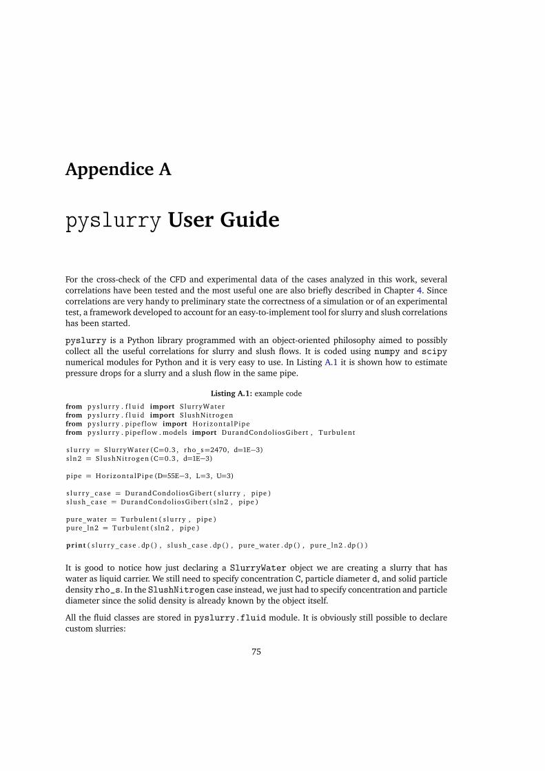
Appendice A
pyslurry User Guide
For the cross-check of the CFD and experimental data of the cases analyzed in this work, severalcorrelations have been tested and the most useful one are also briefly described in Chapter 4. Sincecorrelations are very handy to preliminary state the correctness of a simulation or of an experimentaltest, a framework developed to account for an easy-to-implement tool for slurry and slush correlationshas been started.
pyslurry is a Python library programmed with an object-oriented philosophy aimed to possiblycollect all the useful correlations for slurry and slush flows. It is coded using numpy and scipynumerical modules for Python and it is very easy to use. In Listing A.1 it is shown how to estimatepressure drops for a slurry and a slush flow in the same pipe.
Listing A.1: example code
from pys lu r r y . f l u i d import SlurryWaterfrom pys lu r r y . f l u i d import SlushNitrogenfrom pys lu r r y . p ipef low import Hor izonta lP ipefrom pys lu r r y . p ipef low . models import DurandCondoliosGibert , Turbulent
s l u r r y = SlurryWater (C=0.3 , rho_s=2470, d=1E−3)s ln2 = SlushNitrogen (C=0.3 , d=1E−3)
pipe = Hor izonta lP ipe (D=55E−3, L=3, U=3)
s l u r r y _ c a s e = DurandCondoliosGibert ( s l u r r y , pipe )s lu sh_case = DurandCondoliosGibert ( sln2 , pipe )
pure_water = Turbulent ( s lu r r y , pipe )pure_ln2 = Turbulent ( sln2 , pipe )
print ( s l u r r y _ c a s e . dp () , s lu sh_case . dp () , pure_water . dp () , pure_ln2 . dp () )
It is good to notice how just declaring a SlurryWater object we are creating a slurry that haswater as liquid carrier. We still need to specify concentration C, particle diameter d, and solid particledensity rho_s. In the SlushNitrogen case instead, we just had to specify concentration and particlediameter since the solid density is already known by the object itself.
All the fluid classes are stored in pyslurry.fluid module. It is obviously still possible to declarecustom slurries:
75

Listing A.2: Custom declaration
from pys lu r r y . f l u i d import S lu r ry
cus tom_s lurry = S lu r ry ( rho = f lu id_rho , rho_s = so l id_rho ,C=concentra t ion , mu = l i q u i d _ v i s c o s i t y ,d=p a r t i c l e _ d i a m e t e r )
The module is currently an alpha version, models for Laminar (Poiseuille),Turbulent (Turbulent)pure fluid and non-developed laminar pure fluid (NonDevPoiseuille) are provided together withDurand and Condolios [49] (DurandCondoliosGibert), see Section 4.2, and Yuan and Turian [54],[55] (TurianYuan1977), see Section 4.3, correlations for solid-liquid multiphase flows.
The code will be released soon under a Free and Open Source Software (FOSS) license. Check mygithub profile for updates github.com/rubendibattista.
76

Acronimi
2FM Two-fluids model. 7, 27
AR Aspect Ratio. 7, 49
BC Boundary Condition. 3, 5, 7, 40, 41, 51, 52
CFCs Chlorofluorocarbons. 7, 13
CFD Computational Fluid Dynamics. 7, 27, 56, 63, 70, 75
DNS Direct Navier-Stokes Simulation. 7, 41
DPE Discrete Particle Element. 7, 33
E-E Euler-Euler. 7, 28
E-L Euler-Lagrange. 7, 28
ESA European Space Agency. 7, 9, 11, 13, 19
F-T Freeze-thaw. 7, 19, 21
FDM Finite Difference Method. 7, 28
FESTIP Future European Space Transportation Investigations Programme. 7, 9, 11, 13, 19
FLUSH FLow of slUSH. 7, 43, 45
FOSS Free and Open Source Software. 7, 76
FVM Finite Volume Method. 7, 28
GNU GNU’s not Unix. 7
HRE Hybrid Rocket Engine. 7, 14
JAXA Japan Aerospace eXploration Agency. 7, 9, 11, 13
KTGF Kinetic Theory for granular flows. 7, 27, 28, 35, 49, 54, 69, 79
77
LH2 Liquid Hydrogen. 7, 13, 20, 23, 24, 44
LHS Left Hand Side. 7, 40
LN2 Liquid Nitrogen. 7, 13, 23, 24, 70
LOX Liquid Oxygen. 7, 13
LRE Liquid Rocket Engine. 7, 14
MULES MUlti-dimensionsal Limiter for Explicit Solution. 7, 49
N-S Navier-Stokes. 7, 28, 29
NASA National Aeronautics and Space Administration. 7, 9, 11, 43
NASP National Space Plane. 7, 9, 11, 13, 19, 43
NBPH2 Normal-Boiling-Point Hydrogen. 7
NIST National Institute of Standards and Technology. 7, 45
OpenFOAM Open source Field Operation And Manipulation. 7, 35, 49, 51, 52, 54, 69–71
PIV Particle Image Velocimetry. 7, 42, 69
PoliMI Politecnico di Milano. 7, 71
RANS Reynolds-Averaged Navier-Stokes equations. 7
RHS Right Hand Side. 7, 29, 31
SLH2 Slush Hydrogen. 5, 7, 9, 13, 19–25, 28, 43–45
SLH2O Slurry Ice. 7, 19
SLN2 Slush Nitrogen. 7, 19, 22–24, 28, 49, 62, 70
SLO2 Slush Oxygen. 7, 14, 19, 20
SRM Solid Rocket Motor. 7, 14
TP Triple-point. 7, 19, 44
TPH2 Triple-Point Hydrogen. 7
VKI Von Karman Institute for Fluid Dynamics. 7, 70, 71
78

Latin Symbols
c Particle fluctuating velocity in KTGFCD Drag coefficientCL Lift coefficientCv.m. Virtual Mass coefficient
dp Diameter of a particle
e Coefficient of restitutionew Wall Coefficient of restitution
g Gravity field at sea level
9.81
NKg
g0 Radial distribution function
h Enthalpy per unit of mass
Pf Granular pressure additional term due to frictio-nal stress
k Turbulent kinetic energy
` Reference Length
Mϕ Phase momentum exchange term
p PressurePs Granular pressure
R Reynols stress tensor
u Velocity vectorur Relative velocity between particle and carrier
V Volumevi Velocity of the interface between phasesVp Volume of a particlevt Terminal settling velocity of a particle
79

x Position vector
Yϕ Phase ϕ mass fraction
80

Greek Symbols
αϕ Phase ϕ fraction
χϕ Phase indicator function
δ Angle of friction
ε Turbulent dissipation rate
γ Generic property subjected to operators
κΘ Granular conductivity
λs Bulk viscosity of the granular phase
µ Viscosityµc Carrier liquid viscosityµ f Granular viscosity additional term due to frictio-
nal stressµt Turbulent viscosity
ω Turbulent specific dissipation
φ Specularity coefficient
ρ Density
Σ Surface Area per unit volume
Θ Granular temperature
81


Non-dimensional Groups
F rfl Flow Froude number sortF rp Particle Froude number sort
Co Courant number |u|∆t∆x
Rep Particle Reynolds number ρ|ur |Dµc
Re Reynolds number ρU Dµ
St Stokes number 18µcρpd2
p
UD
83

Bibliografia
[1] C. Sindt, «A summary of the characterization study of slush hydrogen», Cryogenics, vol. 10, n. 5, pp. 372–380, 1970.[2] C. F. Sindt, «Heat transfer to slush hydrogen», in Advances in Cryogenic Engineering, ser. Advances in Cryogenic En-
gineering 19, K. D. Timmerhaus, cur., DOI: 10.1007/978-1-4613-9847-9_52, Springer US, 1995, pp. 427–436, ISBN:978-1-4613-9849-3 978-1-4613-9847-9.
[3] D. B. Mann, P. R. Ludtke, C. F. Sindt e D. B. Chelton, «Liquid-solid mixtures of hydrogen near the triple point», inAdvances in Cryogenic Engineering, Springer, 1966, pp. 207–217.
[4] C. F. Sindt, P. R. Ludtke e D. E. Daney, Slush hydrogen fluid characterization and instrumentation. for sale by the Supt.of Docs., US Govt. Print. Off., 1969, vol. 377.
[5] D. E. Daney, P. R. Ludtke e C. F. Sindt, «Slush hydrogen pumping characteristics using a centrifugal-type pump», inAdvances in Cryogenic Engineering, Springer, 1969, pp. 438–445.
[6] A. Friedlander, R. Zubrin e T. L. Hardy, «Benefits of slush hydrogen for space missions», 1 ott. 1991.[7] S. Zhang. (2 mar. 2016). SpaceX keeps aborting liftoffs because rocket fuel is tricky, WIRED, indirizzo: http://
www.wired.com/2016/03/spacex- keeps- aborting- liftoffs- rocket- fuel- tricky/ (visitato il03/08/2016).
[8] M. A. Karabeyoglu, B. J. Cantwell e D. Altman, «Development and testing of paraffin-based hybrid rocket fuels», AIAApaper, vol. 4503, p. 2001, 2001.
[9] C. T. Crowe, cur., Multiphase flow handbook, ser. Mechanical engineering series, Boca Raton, Fla.: Taylor & Francis,2006, ISBN: 978-0-8493-1280-9.
[10] Y. M. Park, «Literature research on the production, loading, flow, and heat transfer of slush hydrogen», InternationalJournal of Hydrogen Energy, Asian Hydrogen Energy Conference 2009, vol. 35, n. 23, pp. 12 993–13 003, dic. 2010,ISSN: 0360-3199.
[11] S. Gürsu, S. A. Sheriff, T. N. Vezirocglu e J. W. Sheffield, «Review of slush hydrogen production and utilizationtechnologies», International Journal of Hydrogen Energy, vol. 19, n. 6, pp. 491–496, giu. 1994, ISSN: 0360-3199.
[12] K. Ohira, «Pressure drop reduction phenomenon of slush nitrogen flow in a horizontal pipe», Cryogenics, vol. 51, n. 7,pp. 389–396, lug. 2011, ISSN: 0011-2275.
[13] K. Ohira, S. Matsuo e H. Furumoto, «An experimental investigation of production and density measurement of slushhydrogen», Cryogenics, Fifteenth International Cryogenic Engineering Conference, vol. 34, Supplement 1, pp. 397–400, 1994, ISSN: 0011-2275.
[14] H. Fujiwara, M. Yatabe, H. Tamura, M. Takahashi, J. Miyazaki e Y. Tsuruta, «Experiment on slush hydrogen productionwith the auger method», International Journal of Hydrogen Energy, vol. 23, n. 5, pp. 333–338, mag. 1998, ISSN:0360-3199.
[15] R. O. Voth, «Producing liquid-solid mixtures (slushes) of oxygen or hydrogen using an auger», Cryogenics, vol. 25, n.9, pp. 511–517, 1 set. 1985, ISSN: 0011-2275.
[16] M. J. Baker, T. T. Denton e C. Herr, «An explanation for why it is difficult to form slush nitrogen from liquid nitrogenused previously for this purpose», Cryobiology, vol. 66, n. 1, pp. 43–46, feb. 2013, ISSN: 0011-2240.
[17] «Apparatus for making hydrogen slush using nitrogen and helium refrigerants», US3521457 A, U.S. Classification62/54.1, 62/354, 62/467; International Classification F25J1/00; Cooperative Classification F25J1/0072, F25J1/0052,F25J1/001, F25J2210/42, F25J2290/42, F25J1/0221, F25J1/0065, F25J1/0205, F25J2205/20, F25J1/0276; Euro-pean Classification F25J1/02, F25J1/02B4, F25J1/00R4N, F25J1/00C4V, F25J1/02F, F25J1/02Z4U2, F25J1/00R2H,F25J1/00A2W, 21 lug. 1970.
[18] N. B. Mcnelis, T. L. Hardy, M. V. Whalen, M. T. Kudlac, M. E. Moran, T. M. Tomsik e M. S. Haberbusch, «A summaryof the slush hydrogen technology program for the national aero-space plane», presentedatHypersonics TechnologiesConference, Chattanooga, TN, United States, 1 apr. 1995.
[19] K. Ohira, K. Nakamichi e Y. Kihara, «Development of a waveguide-type flowmeter using a microwave method for slushhydrogen», JSME International Journal Series B Fluids and Thermal Engineering, vol. 48, n. 1, pp. 114–121, 2005.
[20] K. Ohira, «Study of nucleate boiling heat transfer to slush hydrogen and slush nitrogen», Heat Transfer—Asian Research,vol. 32, n. 1, pp. 13–28, 1 gen. 2003, ISSN: 1523-1496.
85

[21] Y. Jiang e P. Zhang, «Pressure drop and flow pattern of slush nitrogen in a horizontal pipe», AICHE Journal, vol. 59, n.5, pp. 1762–1773, mag. 2013, ISSN: 00011541.
[22] A. Carapelle e J. .-.-P. Collette, «Gamma-ray attenuation for measuring cryogenic slush mixture density», NuclearInstruments and Methods in Physics Research Section B: Beam Interactions with Materials and Atoms, vol. 229, n. 1,pp. 111–116, feb. 2005, ISSN: 0168-583X.
[23] N. US Department of Commerce. (). NIST XCOM: Photon cross sections database, indirizzo: http://www.nist.gov/pml/data/xcom/ (visitato il 19/02/2016).
[24] K. Ohira, «Development of density and mass flow rate measurement technologies for slush hydrogen», Cryogenics, vol.44, n. 1, pp. 59–68, gen. 2004, ISSN: 0011-2275.
[25] K. Ohira, A. Ota, Y. Mukai e T. Hosono, «Numerical study of flow and heat-transfer characteristics of cryogenic slushfluid in a horizontal circular pipe (SLUSH-3d)», Cryogenics, vol. 52, n. 7, pp. 428–440, lug. 2012, ISSN: 0011-2275.
[26] K. Ohira, K. Nakagomi e N. Takahashi, «Pressure-drop reduction and heat-transfer deterioration of slush nitrogen inhorizontal pipe flow», Cryogenics, vol. 51, n. 10, pp. 563–574, ott. 2011, ISSN: 0011-2275.
[27] R. S. Collier, «Thermally induced oscillations in cryogenic systems», 1972.[28] T. E. Rhafiki, «Modélisation et étude numérique d’un écoulement diphasique solide-liquide subissant un chagement
de phase dans un échangeur de chaleur. application aux coulis de glace et stabilisé», tesi di dott., Université de Pau etdes Pays de l’Adour Pau-France, dic. 2009.
[29] Y. Jiang e P. Zhang, «Numerical investigation of slush nitrogen flow in a horizontal pipe», Chemical Engineering Science,vol. 73, pp. 169–180, mag. 2012, ISSN: 00092509.
[30] J. Ishimoto e R. Ono, «Numerical study of the two-phase flow characteristics of slush nitrogen», Cryogenics, vol. 45,n. 4, pp. 304–316, apr. 2005, ISSN: 0011-2275.
[31] L. Chen, Y. Duan, W. Pu e C. Zhao, «CFD simulation of coal-water slurry flowing in horizontal pipelines», KoreanJournal of Chemical Engineering, vol. 26, n. 4, pp. 1144–1154, lug. 2009, ISSN: 0256-1115, 1975-7220.
[32] D. Kaushal, T. Thinglas, Y. Tomita, S. Kuchii e H. Tsukamoto, «CFD modeling for pipeline flow of fine particles at highconcentration», International Journal of Multiphase Flow, vol. 43, pp. 85–100, lug. 2012, ISSN: 03019322.
[33] J. Wang, T. Zhang e S. Wang, «Heterogeneous ice slurry flow and concentration distribution in horizontal pipes»,International Journal of Heat and Fluid Flow, vol. 44, pp. 425–434, dic. 2013, ISSN: 0142-727X.
[34] D. P. Hill, «The computer simulation of dispersed two-phase flow», tesi di dott., University of London, 1998.[35] P. Crivellari, L. del Monte e F. Gamma, «Computational fluidynamics of hydrogen for aerospace vehicles», 1999.[36] F. Gamma, L. del Monte e R. Liberatore, «CFD-analysis of slush hydrogen flows in feed-systems of rocket-based
combined cycles», in AIAA/ASME/SAE/ASEE Joint Propulsion Conference & Exhibit, 34 th, Cleveland, OH, 1998.[37] P. Reynier, M. Bugel e J. Lecoîntre, «Review of the modelling of slush hydrogen flows», The Journal of Computational
Multiphase Flows, vol. 3, n. 3, pp. 123–146, 1 set. 2011, ISSN: 1757-482X.[38] H. Rusche, «Computational fluid dynamics of dispersed two-phase flows at high phase fractions», tesi di dott., Imperial
College London (University of London), 2003.[39] C. Dopazo, «On conditioned averages for intermittent turbulent flows», Journal of Fluid Mechanics, vol. 81, n. 3,
pp. 433–438, 1977.[40] A. D. Gosman, C. Lekakou, S. Politis, R. I. Issa e M. K. Looney, «Multidimensional modeling of turbulent two-phase
flows in stirred vessels», AICHE Journal, vol. 38, n. 12, pp. 1946–1956, 1992.[41] B. G. M. v. Wachem, «Derivation, implementation, and validation of computer simulation models for gas-solid fluidized
beds», ResearchGate,[42] J. Lundberg e B. M. Halvorsen, «A review of some exsisting drag models describing the interaction between phases in
a bubbling fluidized bed».[43] D. Gidaspow, Multiphase flow and fluidization: Continuum and kinetic theory descriptions. Boston: Acad. Press [u.a.],
1994, 467 pp., ISBN: 978-0-12-282470-8.[44] P. C. Johnson e R. Jackson, «Frictional–collisional constitutive relations for granular materials, with application to
plane shearing», Journal of Fluid Mechanics, vol. 176, pp. 67–93, 1987.[45] D. G. Schaeffer, «Instability in the evolution equations describing incompressible granular flow», Journal of differential
equations, vol. 66, n. 1, pp. 19–50, 1987.[46] S. A. Miedema, «An overview of theories describing head losses in slurry transport: A tribute to some of the early
researchers», in ASME 2013 32nd International Conference on Ocean, Offshore and Arctic Engineering, American Societyof Mechanical Engineers, 2013, V04AT04A038–V04AT04A038.
[47] T. L. Hardy, «Flush: A tool for the design of slush hydrogen flow systems», 1 feb. 1990.[48] J. R. Fowler e R. C. Hendricks, «Computing properties of pure and mixed fluids», 1993.[49] R. Durand e E. Condolios, «Experimental investigation of the transport of solids in pipes», Deuxieme Journée de
lhydraulique, Societé Hydrotechnique de France, 1952.[50] S. Sadat-Helbar, E. Amiri-Tolkadany, Steve Darby e A. Shafaie, «Fall velocity of sediment particles»,[51] R. M. Turian e T.-F. Yuan, «Flow of slurries in pipelines», AICHE Journal, vol. 23, n. 3, pp. 232–243, 1 mag. 1977, ISSN:
1547-5905.[52] R. M. Turian, F.-L. Hsu e T.-W. Ma, «Estimation of the critical velocity in pipeline flow of slurries», Powder Technology,
vol. 51, n. 1, pp. 35–47, 1987.
86
[53] D. Kaushal, K. Sato, T. Toyota, K. Funatsu e Y. Tomita, «Effect of particle size distribution on pressure drop andconcentration profile in pipeline flow of highly concentrated slurry», International Journal of Multiphase Flow, vol. 31,n. 7, pp. 809–823, lug. 2005, ISSN: 03019322.
[54] R. M. Turian, F. L. Hsu e M. S. Selim, «FRICTION LOSSES FOR FLOW OF SLURRIES IN PIPELINE BENDS, FITTINGS,AND VALVES», Particulate Science and Technology, vol. 1, n. 4, pp. 365–392, ott. 1983, ISSN: 0272-6351, 1548-0046.
[55] R. M. Turian, T.-F. Yuan e G. Mauri, «Pressure drop correlation for pipeline flow of solid-liquid suspensions», AICHEJournal, vol. 17, n. 4, pp. 809–817, 1 lug. 1971, ISSN: 1547-5905.
87