numerical simulation of fluidic actuators for flow control

Numerical Simulation of Fluidic Actuators for Flow ControlApplications

Veer N. Vatsa∗ , Mehti Koklu† , Israel L. Wygnanski‡

NASA Langley Research Center, Hampton,VA 23681

andEhab Fares§

Exa GmbH, Stutgart, Germany

Active flow control technology is finding increasing use in aerospace applications to control flow separationand improve aerodynamic performance. In this paper we examine the characteristics of a class of fluidic actua-tors that are being considered for active flow control applications for a variety of practical problems. Based onrecent experimental work, such actuators have been found to be more efficient for controlling flow separation interms of mass flow requirements compared to constant blowing and suction or even synthetic jet actuators. Thefluidic actuators produce spanwise oscillating jets, and therefore are also known as sweeping jets. The frequencyand spanwise sweeping extent depend on the geometric parameters and mass flow rate entering the actuatorsthrough the inlet section. The flow physics associated with these actuators is quite complex and not fully un-derstood at this time. The unsteady flow generated by such actuators is simulated using the lattice Boltzmannbased solver PowerFLOW R©. Computed mean and standard deviation of velocity profiles generated by a fam-ily of fluidic actuators in quiescent air are compared with experimental data. Simulated results replicate theexperimentally observed trends with parametric variation of geometry and inflow conditions.

Nomenclature

D divergence angle, degreeslb poundm metermdot mass flow rate, lb/secmm millimeterk turbulence kinetic energypsi pound per square inchs, sec secondt time, secondsV velocity magnitudeVavg time-averaged velocity magnitudeV′rms root-mean square of perturbation velocityVtotal instantaneous total velocityx,y,z Cartesian coordinates3-D three-dimensionalε dissipation length scale

∗Senior Research Scientist, Computational AeroSciences Branch, Research Directorate; Associate Fellow AIAA†Aerospace Engineer, Flow Physics and Control Branch, Research Directorate; Member AIAA‡Senior Aerodynamicist, Flow Physics and Control Branch, Research Directorate; Fellow AIAA§Technical Manager, Aerospace Applications, Exa GmbH; Senior Member AIAA

1 of 17

https://ntrs.nasa.gov/search.jsp?R=20120011819 2019-04-13T07:32:58+00:00Z

Abbreviations:AFC active flow controlCFD computational fluid dynamicsDNS direct numerical simulationERA environmentally responsible aviationLBM lattice Boltzmann methodVR variable resolution

Superscript:◦ angle in degrees′ perturbation quantity (e.g. V′ = V-Vavg)

Subscript:0 initial value

I. Introduction

There has been a growing emphasis on reducing the fuel burn of commercial aircraft to meet the stringent restrictionson emissions and noise imposed by regulatory agencies. A significant effort is being devoted to such activities at NASAthrough the Environmentally Responsible Aviation (ERA) program. One area of research under this program is toincrease the lift/drag ratio and/or reduce the size of control surfaces on aircraft by making use of active flow control(AFC) devices, which will decrease the overall weight of the aircraft. The AFC devices have to be designed to maximizeperformance with the least amount of weight penalty and power requirements. In addition, these devices must haveacceptable fault tolerance.

Recent advances in computational fluid dynamics (CFD) methods have made it possible to simulate the effect ofactive flow control devices on major aircraft components, as evidenced by a series of publications in the literature.1–5

The paper of Collis et al.4 summarizes the various issues encountered in active flow control applications from boththeoretical and experimental points of view. Until recently, flow control was achieved primarily with synthetic or pulsedjet actuators. All of these devices consist of moving parts and controllers, which can cause operational problems inflight.

During the last several years, fluidic actuators have come to prominence as viable flow control devices for improvingthe aerodynamic performance of high lift configurations by mitigating separated flow regions. Such devices do notcontain any moving parts and rely primarily on the feedback mechanism triggered by the unsteady flow inside theactuators. DeSalvo et al.6 and Woszidlo and Wygnanski7 have examined the performance of such actuators in recentpapers. Based on the available research, it appears that the fluidic actuators that produce spanwise oscillating or sweepingjets offer a reliable and efficient mechanism for active flow control applications.

CFD simulations are used here to examine the internal and external flow structures created by fluidic actuatorsoperating in quiescent air. Numerical studies are conducted to quantify the effect of geometric shape changes and inputconditions on the performance characteristics of such actuators. The computed solutions are compared with availableexperimental data for several configurations.

II. Configurations

The fluidic actuators under consideration here are closely related to the ones examined by Gokoglu et al.8–10 Theprimary difference in the current configuration is the absence of the divider section used in their work to create twinoutlets for the fluid to exit. In the current configuration, which is simpler to fabricate and is being used in severalpractical applications, the jet comes out of a single outlet, as sketched in Fig. 1. Here the x-coordinate aligns with theprimary jet flow direction, whereas the z-coordinate refers to the spanwise direction. The y-coordinate is out of the paperin this figure and is normal to the x-z plane. Some of the geometric details are suppressed here (covered by gray regionsin Fig. 1) because of the proprietary nature of the device.

The inflow boundary is connected to a high pressure source to inject a constant supply of air into the actuator. Thepressure differential between this air supply and the ambient atmosphere sets up a constant mass flow through the inflowsection. The mass flow going through the actuator is directly proportional to the pressure differential, or gauge pressure.The flow accelerates up to the first nozzle before entering the main chamber, which contains constrictions placed on

2 of 17

American Institute of Aeronautics and Astronautics Paper 2010-4001

the left and right sides, sub-dividing the main chamber. Due to the shape of this geometry, an oscillating unsteady flowdevelops inside the chamber such that in addition to the flow exiting through the second nozzle near the exit plane,there exists a backflow moving between the left and right side of the chamber. As a result, the flow exiting this nozzleoscillates from left to right in a cyclic pattern. The frequency and the spanwise extent of the oscillatory jet depend onthe precise shape of the actuator and pressure differential between the inflow boundary and the ambient atmosphere.

We consider two types of fluidic actuators in this paper. The first type are formed with straight edges, sharp corners,and planar surfaces. The divergence angle of the exit nozzle for the baseline configuration, shown schematically inFig. 1, is 124◦. The divergence angle of exit nozzle for the second actuator of this type under consideration is 90◦. Flowcharacteristics of similar actuators have been examined by Gokoglu et al. in a series of papers.8–10 These will be referredto as Type I, 124D and 90D actuators, or for simplicity as 124D and 90D actuators.

We also examine another type of fluidic actuator in this paper where the internal chamber consists of smooth curvededges instead of sharp corners and edges, as shown in Fig. 2. Woszidlo and Wygnanski discussed the geometric detailsand origins of such actuators in a recent paper.7 At the start of the process (t = t0), the jet attaches to either wall ofinterior cavity, shown schematically in Fig. 2. The curving of the jet increases the pressure at the feedback channel inletand induces reverse flow in the feedback channel that pushes the jet to the opposite side at a later time, t = t0 + dt. Theprocess repeats itself at a frequency set by the precise shape of the actuator and the inlet conditions. A series of suchactuators were embedded in a high-lift configuration consisting of a NACA 0021 airfoil with variable flap geometry.The effectiveness of these actuators to control the separated region for such airfoils was clearly demonstrated in Ref. 7,where significant improvement in measured lift was achieved with flow control compared to the baseline configuration.These actuators will be referred to as Type II curved-wall actuators, or as just curved-wall actuators for simplicity.

III. Experimental Setup

The fluidic actuators described in the previous section have been manufactured at NASA Langley Research Centerand are being tested in a bench-top environment. A photograph of the curved-wall actuator model under consideration isshown in Fig. 3. A high pressure air supply is attached to the inlet boundary and the flow exits from the outlet face intoquiescent air of the room. The mass flow entering the actuator and the magnitude of the exit velocity depend strongly onthe pressure differential between the inflow plane and the ambient atmosphere. The mass flow rate entering the actuatoris measured with a flow meter placed inline with the air supply tubing. A static pressure probe placed inside the inletsection is used to measure the inflow pressure. Hot-wire measurements are taken at several locations downstream of theexit plane. The raw data is processed to generate a time-series of the velocity signal. In addition to the instantaneous andmean velocities, the root mean square (rms) or standard deviation of the perturbation velocities are also extracted fromthe hot-wire data.

Fluidic actuators of different depths have been fabricated and tested at NASA Langley. However, the results presentedin this paper correspond to the actuators that are 0.25 inches (6.35 mm) deep. The throat width of the exit nozzle is nearlyequal in size to the depth for these actuators. Therefore, the aspect ratio of the rectangular throats for these actuators isapproximately one.

IV. Simulation Method

The numerical simulations presented in this paper were performed using the commercial software PowerFLOW R©

(version 4.3) which is based on the three dimensional 19 state (D3Q19) lattice Boltzmann model. The lattice Boltzmannmodel (LBM) can be derived from the velocity space discretization of the general Boltzmann equation, and it recoversthe full unsteady Navier–Stokes equations.11–14 The lattice Boltzmann equation can be solved in a DNS mode, where allof the turbulent scales are spatially and temporally resolved. However, for most engineering problems at high Reynoldsnumbers, the simulations are usually conducted in conjunction with a hybrid turbulence modeling approach where thesmall scales are modeled using a modified two-equations k−ε turbulence model and larger energy containing scalesare directly resolved. The turbulence model uses a swirl correction to locally reduce the influence of the modelededdy viscosity to allow vortical structures to develop and persist without added artificial damping.15–17 In addition, awall model relying on algebraic general relations such as the logarithmic law of the wall, and extended to account forpressure gradients effects is used to capture the boundary layer behavior and relax the grid spacing requirement nearthe solid walls.18 The turbulence modeling approach together with the inherently unsteady nature of the LBM ensuresaccurate and efficient simulation of the large structures especially in regions of separated flows and shows conceptualsimilarities with the recent DDES approach of Spalart.19 This was the approach used for obtaining numerical solutionspresented in this paper.

3 of 17


The lattice Boltzmann equation is solved on embedded Cartesian meshes, which are generated automatically withinthe flow solver for the configuration under consideration, irrespective of the geometric complexity. Furthermore, vari-able refinement regions (VR) can be defined to allow for local mesh refinement of the grid size by successive factorsof two in each direction.20 The PowerFLOW R©code scales well on highly parallel clusters using up to thousands ofprocessors, making it ideally suitable for large scale applications. The LBM used here has been extensively validatedfor a wide variety of applications ranging from academic cases using DNS21 to industrial flow problems in the fields ofaerodynamics, thermal management, and aeroacoustics, see e.g. Refs. (5, 17, 22, 23).

A cross section of the computational grid (lattices) for the Type II, curved-wall actuator used in the PowerFLOW R© sim-ulations is shown in Fig. 4. The 3-D computational domain consists of hexahedral voxels formed by extruding the 2-Dgrid in the y-direction. The volumetric mesh is very coarse in the outer region, which is essentially a quiescent (no flow)region and becomes successively finer as the computational boxes get closer to the actuator. The finest grids are usednear the solid walls to resolve the high gradient viscous regions. The grid for this case consisted of a total of 29.7 millionvoxels (cells) distributed among 6 VR regions. Similar grids were created for the Type I actuator simulations.

V. Results

The unsteady 3-D flow fields created by the fluidic actuators exhausting into quiescent air were computed using theThe PowerFLOW R©code. The baseline conditions chosen for this work correspond to an inlet mass flow of 0.015 lb/secat room temperature. Viscous wall conditions were imposed on all of the solid walls that form the actuator geometry andthe internal components. A back pressure of 14.7 psi was imposed at the outflow boundary. Frictionless wall boundaryconditions were imposed at rest of the computational boundaries.

The computations were run for large number of time steps to generate a database from which statistically convergedmean and perturbation flow quantities could be extracted. Instantaneous flow field data was collected at various locationscorresponding to experimental measurement locations downstream of the actuator exit. Computed time-averaged meanand perturbation velocities for three different actuators are compared with the measured data. These results are discussedin the following sub-sections.

A. Type I, 124D actuator

The first test case chosen for numerical simulations is the baseline 124D actuator which produces a sweeping jet thatoscillates in the spanwise direction, z. To compare the performance and characteristics of such actuators with the onesthat produce planar (non-sweeping) jets, the baseline configuration was modified as follows. Two 10 mm long solidblocks shown schematically as blue rectangles in Fig. 1, were inserted between the external walls and the internal diverterblocks on both sides to block the feedback channel. Although the flow field associated with this modified configurationis still unsteady in nature, the insertion of these solid blocks had the desired effect of creating an exit jet that residesmostly near the mid-section, instead of oscillating in the spanwise direction. The velocity magnitude contours from thenumerical simulations for the modified configuration are shown in Fig. 5. Notice that the jet stays close to the centerfor this case. These additional solid blocks were then removed to recover the original baseline actuator configuration.The computational results for the original 124D configuration verify the presence of sweeping jet oscillating from leftto right. Instantaneous velocity contours at two different times from these simulations are shown in Fig. 6. Results inFig. 6 (a) indicate that most of the flow exiting the nozzle of the actuator at this instant in time is leaning towards the leftside, thus leaving the flow on right side essentially undisturbed. The situation is exactly reversed in Fig. 6 (b), where thejet is leaning to the right. Time animation of these results (not shown here) is even more helpful in demonstrating theunderlying flow patterns and the highly unsteady nature of the flow for these cases.

The time-averaged and root mean square (rms) perturbation velocity profiles at the x=6 mm location for these casesare compared with the experimental data in Fig 7. The perturbation velocities shown in this figure have been normalizedfor each data set with the corresponding maximum average velocity. For the configuration with blocked feedback chan-nel, the maximum value of time-averaged velocity is almost 50% larger compared to the baseline 124D configuration.The opposite trend is observed for the normalized perturbation velocities (V′rms) in Fig. 7 (b), where the peak valuesfor the blocked channel configuration are seen to be nearly half of the values attained for the baseline configuration.The predicted velocity peak value for the original 124D configuration is slightly higher compared to the measurements,while the situation is reversed for the blocked channel case. Nonetheless, the overall agreement of the computed averagevelocity profiles with measurements is quite good. Note that the predicted velocity profiles are fuller (broader) in shapefor both of these cases compared to the experimentally measured profiles.

Although the perturbation velocities are under-predicted for both cases, the computed profiles replicate the shape andthe most salient features of the measured profiles quite well, including the twin off-center peaks and a local minimum at

4 of 17


the centerline, z=0. The twin off-center peaks shown in these figures indicate that the most unsteady or energetic part ofthe exit jet occurs away from the centerline. Note that the maximum levels for the perturbation velocities for the blockedfeedback channel configuration are approximately 20–25% of the corresponding mean velocity levels, which is typicalof free jets.24, 25 On the other hand, the perturbation velocities for the baseline 124D sweeping jet are almost twice aslarge, which indicates that the sweeping jets are more energetic in nature, and are accompanied by higher levels of flowunsteadiness.

Next we show the evolution of velocity profiles with the downstream distance x for the baseline 124D case in Fig. 8,where the computed time-averaged and perturbation velocities are compared with the experimental data at x= 6, 12, and18 mm stations. As expected, the peak velocities drop in magnitude with increasing value of downstream distance x, andthe velocity profiles become fuller by spreading out in the spanwise direction. The simulations over-predict the averagevelocities and under-predict the perturbation velocities by approximately 10–15% compared to measured data. Thelargest differences are observed at the x=18 mm location, where the experimental data displays significant asymmetryaround centerline. Even though there are quantitative differences in computed and measured velocities, it is important tonote that the computations predict the correct general trends, which can be very useful for conducting parametric studies.

The final set of results for the 124D configuration examines the effect of varying the mass flow rate flowing throughthe actuator. Experimental data at x=6 mm location is also available for the mass flow rates of 0.010 and 0.020 lb/secfor this configuration. The numerical simulations indicate that both of these mass flow rates produce sweeping jets. Thevelocity profiles showing the effect of varying the mass flow rates are shown in Fig. 9 at x= 6 mm. As seen in earlierresults, the computed profile shapes are fuller compared to experimental results. The average velocities are in fairlygood agreement with the measurements except for the mass flow rate of 0.020 lb/sec. The perturbation peak velocitiesfor all three mass flow rates are under-predicted by approximately 10–20% compared to measured values. However,the general shape of the perturbation velocity profiles and trend with variation in mass flow are similar to the measureddata. Once again, the biggest differences are observed for the higher mass flow rate (0.020 lb/sec) case. It is not clear ifcompressibility effects or some other factors at the higher speeds encountered for the larger mass flow rate cause thesedifferences.

B. Type I, 90D actuator

Computations were also performed for the actuator with 90◦ divergence angle for a mass flow rate of 0.015 lb/sec. Thetime-averaged velocity profiles are compared with the experimental data in Fig. 10 at a distance of 6 and 12 mm fromthe exit plane. The velocity peaks for this case are slightly over-predicted. Overall comparisons at the 6 mm locationare quite good. However, at the 12 mm location, the experimental data displays an asymmetric plateau region in themid-section for mean profiles, a feature that has not been observed in any of the results for the 124D configuration. Thecause of such different behavior is not clear at this point, and it might be worth repeating the experiment for this case.Except in this mid-section region, the agreement between the computed and experimental results is quite good.

The next set of results shows the effect of decreasing the divergence angle of the actuator from 124 to 90 degrees.Fig. 11 (a) shows the comparison of time-averaged velocities normalized by their respective peak levels for the 90D and124D configurations at a distance of 6 mm from the exit plane. The velocity profiles are broader in shape for the 90Dcase compared to the 124D case, which is indicative of larger jet width. In addition, based on the results shown in Fig. 11(b), where the peak mean velocities are plotted as a function of distance x, it is clear that a reduction in the divergenceangle of the actuator causes the peak velocities to decrease. The computational results for the time-averaged velocitiesare in general higher for both configurations compared to the measured values. Except for the station closest to exitplane (x=3 mm), the measured and experimental curves are nearly parallel to each other indicating good agreement fordecay rates of mean velocities with downstream distance x. It is conjectured that measurements at the x= 3 mm location,which is very close to the actuator could suffer from interference effects between the hot-wire probe and the actuatorsurface. It is encouraging to note that the effect of varying the divergence angle on peak levels is also well predicted formean velocities as indicated by the incremental shift in the curves shown in Fig. 11 (b).

C. Type II, curved-wall actuator

The next set of results presented here correspond to the Type II, curved-wall actuator that was shown in Figs. 2–3, andbelong to the class of devices that are currently being used in practical flow control applications to mitigate separatedflow regions.6, 7 Time-averaged and perturbation velocities for this configuration are presented in Figs. 12(a) and (b) atx= 6 mm, where the computed and measured velocity profiles are compared. Results from the 124D case discussed inthe earlier section are also added to these figures for comparison. The velocities presented in these figures have beennormalized by the corresponding maximum time-averaged velocities for each case. Several observations can be drawn

5 of 17


from the results shown in Fig. 12. First of all, the computed profile shapes are in good agreement with their experimentalcounterparts for both the average, and the perturbation (rms) velocities. The normalized perturbation velocities areunder-predicted by approximately 10% compared to measurements. The computations also predict the correct trendsbetween the 124D and curved-wall actuators. For example, the mean and perturbation velocities for the curved-wallactuator are much broader in shape compared to the 124D actuator. Also note that as a fraction of mean velocities, theperturbation velocities for the curved-wall actuator are nearly twice in magnitude when compared to the 124D case. Thelarger spanwise footprint and higher perturbation velocities produced by the curved actuators potentially make thesemore effective devices for flow control applications.

Note that for the Type II curved-wall actuator, the velocity profiles display different trends when compared to theType I actuators that were formed with straight edges and sharp corners discussed in previous figures. For example, thetwin off-center peaks and a sizable dip in the middle is observed in the velocity profiles for the curved-wall actuator incontrast to the single velocity peak at the jet centerline for Type I actuators discussed earlier in the paper. To understandthe reason for such significant differences in jet characteristics of these actuators, the experimentally measured timehistory of the velocity magnitude at z=0 and 10 mm, and x=6 mm for the baseline Type I, 124D actuator is comparedwith the corresponding results for the Type II, curved-wall actuator in Fig. 13. The velocity variation with time forthese two type of actuators display very different patterns. For the 124D actuator, the jet velocity at centerline (z=0)spends considerable time at the higher levels before dropping in magnitude. In contrast, the jet velocity at centerlinefor the curved-wall actuator stays at the higher values very briefly, then drops in magnitude and stays at low values forextended periods. On the other hand, at the off-center (z=10 mm) location, the velocities for the curved-wall actuatorspend approximately equal time between the high and low values as seen in Fig. 13 (b). Also note that the peak velocitylevels for the curved actuator at z=10 mm are almost twice in magnitude when compared to the 124D actuator results. Itis apparent from these velocity signals that the curved-wall actuator jet spends more time at the outer edges of the activeregion and passes very quickly over the centerline, thus creating twin peaks at the two ends and a dip in the velocity nearthe centerline.

Next, the internal and external flow fields associated with the fluidic actuators are examined to improve our under-standing of the underlying flow physics for such devices. For the curved-wall actuator under consideration here, theinstantaneous velocity magnitude contours from numerical simulations are shown in Figs 14 at the mid-plane (y=0)passing through the computational domain. The velocity vectors are also shown in these figures to delineate the instan-taneous flow direction. Fig. 14 (a) corresponds to the time when the jet is aligned with left side of the exit wall. Notethat when the jet aligns with the left side, it forces some of the fluid to enter the right side of the feedback channel andcreates a low speed region on the left side. The curving of the jet in this position increases the pressure in the left sectionof the chamber, which pushes the jet towards the right side. The exact opposite flow pattern develops inside the chamberwhen the jet aligns with the right side at a different time during the simulation cycle as shown in Fig. 14 (b). Such acyclic, bi-modal process sets up an oscillatory jet emanating from the nozzle exit, which in turn can energize the outerflow and enhance the aerodynamic performance of control surfaces, as demonstrated in Ref. 7.

Finally, we examine the behavior of the peak velocities as a function of distance x, measured from the actuator exitplane for the curved-wall actuator. These comparisons for the time-averaged mean velocities are presented in Fig. 15for x varying from 3 to 24 mm. The results for the baseline 124D actuator are also shown in this figure for comparisonpurposes. The computed velocities for the curved-wall actuator are substantially smaller compared to the measured data,the largest differences occurring near the exit plane. The differences become smaller with increasing values of x. Notethat the peak velocity magnitudes for the 124D case are much larger compared to the curved actuator case for the samemass flow rate. However, as seen in the Fig. 12, the curved-wall actuator produces a much fuller profile that spreadsover a larger spanwise extent in the field. The CFD results presented here display the correct qualitative and quantitativetrends in velocity profiles with variation in geometric shape for the two different type of actuators examined here.

D. Jet characteristics

From the flow-control perspective, it is important to examine and understand key properties of the jet flow produced bythe AFC devices. These include the frequency and width of the oscillating jets. The frequency plays an important rolein how quickly the jet mixes with the outer flow, whereas the jet width is representative of the extent of the physicaldomain occupied by the most energetic and unsteady part of the outflowing jet. Such quantitative parameters are helpfulin conducting parametric studies to compare the relative efficiency of different AFC devices. Effect of geometric andinput parameters on these quantities are discussed in the following section.

During the simulations performed with the PowerFLOW R©code, significant amount of time-dependent data were col-lected in pre-selected regions and at probe locations to construct the time-series, and to extract the oscillation frequencyusing spectral analysis. In the experimental work, hot-wire data for instantaneous velocities were collected along pre-

6 of 17


selected rake locations to extract statistical information. A close examination of the spectra obtained from the unsteadydata indicates the existence of a primary frequency that contains the most significant energy content, and hence it is themost important frequency for comparing relative characteristics of such devices. The primary frequency of oscillationsat x=6 and z=10 mm probe location obtained from the experimental data and simulations are compared in Fig. 16 forthe 124D and curved-wall actuators corresponding to mass flow rates of 0.010, 0.015 and 0.020 lb/sec. As expected,the oscillation frequency increases with the mass flow rate due to increase in flow velocities. The predicted frequenciesare somewhat higher compared to their measured counterparts, but replicate the experimentally observed trends withthe variation in mass flow rate fairly well. Except for the lowest mass flow rate (mdot=0.010 lb/sec), the simulated andmeasured frequencies for the curved-wall actuator are slightly lower compared to the baseline 124D case.

Final results presented here compare the growth of jet half-width with the downstream distance x. The jet half-widthis defined as the distance between two points where the mean velocity drops from the maximum to half of that value.For the curved-wall actuator that produce twin peaks in the velocity profile, we take the average of the left and right sidejets. The jet half-widths for the 124D and curved-wall actuators are plotted as a function of distance x in Fig. 17. TheCFD results for the jet width are in excellent agreement with the measured data. The computational results also correctlypredict the increment in jet width due to configuration change from the 124D to the curved-wall actuator.

VI. Concluding Remarks

Numerical simulations have been performed using the PowerFLOW R© code to compute the unsteady flow fieldgenerated by a family of fluidic actuators. These simulations provide useful information about the flow physics inthe internal and external regions of the fluidic actuators. The bi-stable feedback mechanism that produces sweeping,oscillatory jets is demonstrated with the help of computed flow field plots. The present results also demonstrated thatblocking the feedback channel inhibited the sweeping action of outflowing jets.

The effect of varying the inflow mass flow rate, as well as key geometric shape parameters on the jet velocity profileand spanwise spreading rate were presented. Overall agreement of the computed time-averaged mean and perturbationvelocities with measurements for the Type I, sharp-edged actuators was quite good. For the curved-wall actuators ofType II, the mean and perturbation velocities were under-predicted by about 25% near the exit plane, the agreementimproving with downstream distance. The simulations replicated the correct overall trends and profile shapes whencompared with the experimental data.

The primary frequency of oscillation of the sweeping jets produced by these fluidic actuators were extracted from theunsteady data using spectral analysis. The computed frequencies compare favorably with measured values and displayedthe correct trends with respective variation of input mass flow rate. Results were also presented for jet half-width for thebaseline mass flow rate of 0.0150 lb/sec, where the computed jet widths for both the sharp-edged 124D actuator and thecurved-wall actuator were found to be in excellent agreement with the measured data. It was observed from these resultsthat for the same inflow mass flow rate, the Type II fluidic actuator with curved-wall interior geometry produced muchhigher spreading rate for the outflowing jet, and is potentially a better performing device for flow control applications.

Future work will focus on simulating the effect of a series of fluidic actuators on external flow over an aerodynamicconfiguration of practical interest to examine the effectiveness of such AFC devices for separation control. Parametricstudies will be conducted to determine the optimum spacing between actuator arrays to achieve the desired controlauthority with minimum mass flow. An effort will be made to investigate the feasibility of simultaneously simulating theinstalled actuators or formulating suitable boundary conditions to approximate the effect of such devices on the externalflow field in order to improve computational efficiency.

VII. Acknowledgments

This work was supported by NASA’s Fundamental Aerodynamics and Integrated Systems Research Programs throughthe Environmentally Responsible Aviation Project. The first author would also like to acknowledge support provided byMr. Scott Brynildsen of Vigyan Inc. for the geometric modeling of the configurations examined here.

References1Shmilovich, R. and Yadin, Y., “Flow Control for the Systematic Buildup of High-Lift Systems,” Journal of Aircraft, Vol. 45, No. 5, September-

October 2008, pp. 1680–1688.2Shmilovich, R. and Yadin, Y., “Flow Control Techniques for Transport Aircraft,” AIAA Journal, Vol. 49, No. 3, March 2011, pp. 489–502.3Rumsey, C., Gatski, T., Sellers III, W., Vatsa, V., and Viken, S., “Summary of the 2004 Computational Fluid Dynamics Validation Workshop

on Synthetic Jets,” AIAA Journal, Vol. 44, No. 2, 2006, pp. 194–207.

7 of 17


4Collis, S., Joslin, R., Seifert, A., and Theofilis, V., “Issues in active flow control: theory, control, simulation and experiment,” Progress inAerospace Sciences, Vol. 40, No. 4-5, 2004, pp. 237–289.

5Bres, G., Fares, E., Williams, D., and Colonius, T., “Numerical Simulations of the Transient Flow Response of a 3D, Low-Aspect-Ratio Wingto Pulsed Actuation,” AIAA Paper 2011-3440, June 2011.

6DeSalvo, M., Whalen, E., and Glezer, A., “High-Lift Enhancement using Fluidic Actuation,” AIAA Paper 2010-0863, January 2010.7Woszidlo, R. and Wygnanski, I., “Parameters Governing Separation Control with Sweeping Jet Actuators,” AIAA Paper 2011-3172, June 2011.8Gokoglu, S., Kuczmarski, M., Culley, D., and Raghu, S., “Numerical Studies of a Fluidic Diverter for Flow Control,” AIAA Paper 2009-4012,

June 2009.9Gokoglu, S., Kuczmarski, M., Culley, D., and Raghu, S., “Numerical Studies of a Supersonic Fluidic Diverter Actuator for Flow Control,”

AIAA Paper 2010-4415, June 2010.10Gokoglu, S., Kuczmarski, M., Culley, D., and Raghu, S., “Numerical Studies of an Array of Fluidic Diverter Actuators for Flow Control,”

AIAA Paper 2011-3100, June 2011.11Chen, H., Chen, S., and Matthaeus, W., “Recovery of the Navier-Stokes Equations Using a Lattice-gas Boltzmann Method,” Phys. Rev. A,

Vol. 45, 1992, pp. 5339–5342.12Chen, H., Teixeira, C., and Molvig, K., “Digital Physics Approach to Computational Fluid Dynamics, Some Basic Theoretical Features,” Intl.

J. Mod. Phys. C, Vol. 8, No. 4, 1997, pp. 675–684.13Chen, S. and Doolen, G., “Lattice Boltzmann Method for Fluid Flows,” Ann. Rev. Fluid Mech., Vol. 30, 1998, pp. 329–364.14Shan, X., Yuan, X., and Chen, H., “Kinetic Theory Representation of Hydrodynamics: a way beyond the Navier–Stokes equation,” J. Fluid

Mech., Vol. 550, 2006, pp. 413–441.15Chen, H., Kandasamy, S., Orszag, S., Shock, R., Succi, S., and Yakhot, V., “Extended Boltzmann Kinetic Equation for Turbulent Flows,”

Science, Vol. 301, No. 5633, 2003, pp. 633–636.16Chen, H., Orszag, S., Staroselsky, I., and Succi, S., “Expanded Analogy between Boltzmann Kinetic Theory of Fluid and Turbulence,” J. Fluid

Mech., Vol. 519, 2004, pp. 307–314.17Fares, E. and Nolting, S., “Unsteady Flow Simulation of a High-Lift configuration using a Lattice Boltzmann Approach,” AIAA Paper 2011-

869, January 2011.18Teixeira, C., “Incorporating Turbulence Models into the Lattice-Boltzmann Method,” Intl. J. Mod. phys. C, Vol. 9, 1998, pp. 1159–1175.19Spalart, P., Deck, S., Shur, S., Strelets, M., and Tavin, A., “A New Version of DES Resistant to Ambiguous Grid Densities,” Theoretical and

Computational Fluid Dynamics, Vol. 20, No. 3, 2006, pp. 181–195.20Chen, H., “Volumetric Formulation of the Lattice Boltzmann Method for Fluid Dynamics: Basic Concept,” Phys. Rev. E, Vol. 58, 1998,

pp. 3955–3963.21Li, Y., Shock, R., and Chen, H., “Numerical Study of Flow Past an Impulsively Started Cylinder by Lattice Botzmann Method,” J. Fluid Mech.,

Vol. 519, 2004, pp. 273–300.22Fares, E., “Unsteady Flow Simulation of the Ahmed Reference Body using a Lattice Boltzmann Approach,” Comput. Fluids, Vol. 35, No. 8-9,

2006, pp. 940–950.23Bres, G. A., Wessels, M., and Noelting, S., “Tandem Cylinder Noise Predictions Using Lattice Boltzmann and Ffowcs Williams – Hawkings

Methods,” AIAA Paper 2010-3791, 2010.24Bradbury, L., “The Structure of a Self-Preserving Turbulent Plane Jet,” J. of Fluid Mech., Vol. 23, 1965, pp. 31–64.25Gutmark, E. and Wygnanski, I., “The Planar Turbulent Jet,” J. of Fluid Mech., Vol. 73, 1976, pp. 465–495.

8 of 17


Figure 1. Schematic of Type I, 124D fluidic actuator, top view.

t=t0 t=t0 + dt

Figure 2. Schematic of Type II, curved actuator, top view.

9 of 17


Figure 3. Experimental set-up for Type II curved actuator.

Figure 4. Schematic of PowerFLOW R© computational domain for Type I fluidic actuator.

10 of 17


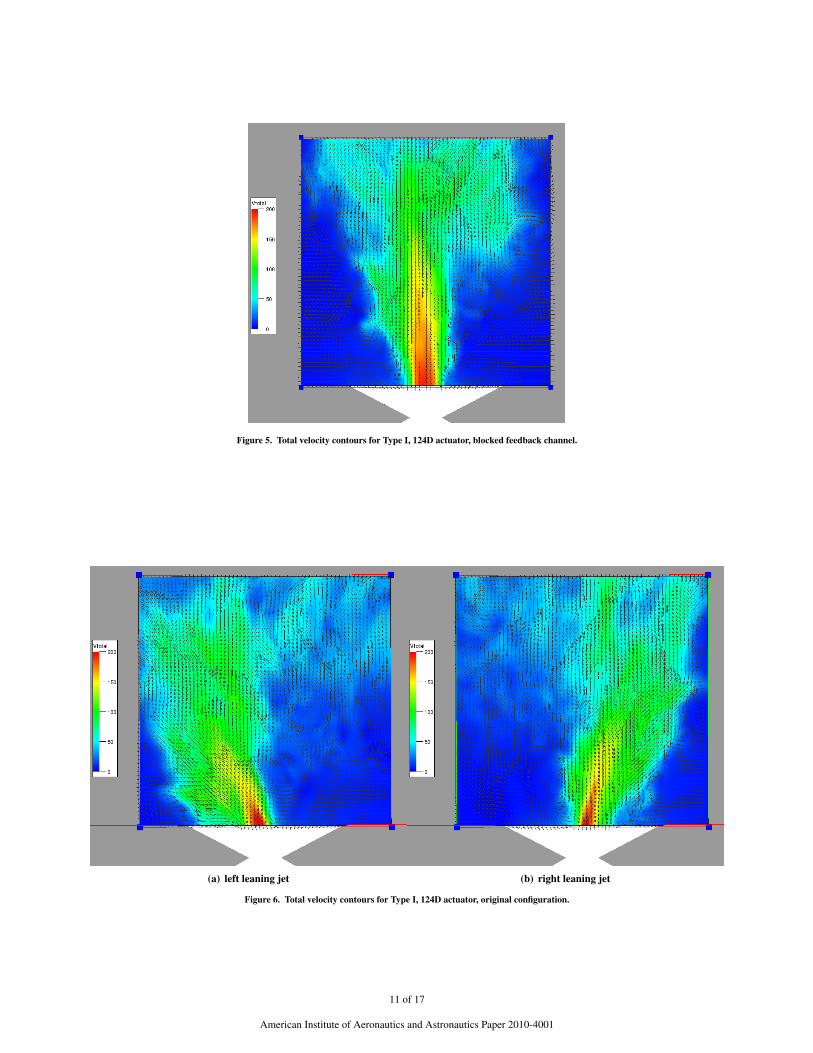
Figure 5. Total velocity contours for Type I, 124D actuator, blocked feedback channel.

(a) left leaning jet (b) right leaning jet

Figure 6. Total velocity contours for Type I, 124D actuator, original configuration.

11 of 17


(a) time-averaged velocities (b) perturbation velocities

Figure 7. Effect of blocked feedback channel on velocity profiles for Type I, 124D actuator, x=6 mm.


Figure 8. Evolution of time-averaged and perturbation velocities for Type I, 124D actuator.

12 of 17



Figure 9. Effect of varying mass flow rate on velocity profiles for Type I, 124D actuator, x=6 mm.

Figure 10. Time-averaged velocity comparisons for Type I, 90D actuator.

13 of 17


(a) mean velocity profiles (b) decay of mean velocities with x

Figure 11. Effect of divergence angle on mean velocities for Type I actuators, x=6 mm.


Figure 12. Normalized velocity comparisons for Type I 124D and Type II curved-wall actuators at x=6 mm, mdot=0.015 lb/sec.

14 of 17


(a) z = 0 mm

(b) z = 10 mm

Figure 13. Time variation of velocities at x=6 mm, experimental data.

15 of 17


(a) left leaning jet (b) right leaning jet

Figure 14. Total velocity contours for Type II, curved-wall actuator, m=0.015 lb/sec.

Figure 15. Decay of peak velocities with x-distance for Type II, curved actuator, mdot=0.015 lb/sec.

16 of 17


Figure 16. Frequency variation with mass flow rate for 124D and curved-wall actuators.

Figure 17. Comparison of jet half-widths for 124D and curved-wall actuators, mdot=0.015 lb/sec.

17 of 17


numerical simulation of fluidic actuators for flow control

Documents