University of Texas at El PasoDigitalCommons@UTEP

Open Access Theses & Dissertations

2014-01-01

Numerical Prediction Of Collection Efficiency OfA Personal Sampler Based On Cyclone PrincipleAntara BadhanUniversity of Texas at El Paso, abadhan@miners.utep.edu

Follow this and additional works at: https://digitalcommons.utep.edu/open_etdPart of the Mechanical Engineering Commons

This is brought to you for free and open access by DigitalCommons@UTEP. It has been accepted for inclusion in Open Access Theses & Dissertationsby an authorized administrator of DigitalCommons@UTEP. For more information, please contact lweber@utep.edu.

Recommended CitationBadhan, Antara, "Numerical Prediction Of Collection Efficiency Of A Personal Sampler Based On Cyclone Principle" (2014). OpenAccess Theses & Dissertations. 1203.https://digitalcommons.utep.edu/open_etd/1203

NUMERICAL PREDICTION OF COLLECTION EFFICIENCY OF A

PERSONAL SAMPLER BASED ON CYCLONE PRINCIPLE

ANTARA BADHAN

Department of Mechanical Engineering

APPROVED:

Shaolin Mao, Ph.D., Chair

Norman Love, Ph.D.

Grace Yan, Ph.D.

Charles H. Ambler, Ph.D.

Dean of the Graduate School

Copyright

by

Antara Badhan

2014

Dedication

To my father M. A. Rahman, my mother Nurzahan Begum & my husband Mohammad Arif

Ishtiaque Shuvo for their support and encouragement throughout my life.

NUMERICAL PREDICTION OF COLLECTION EFFICIENCY OF A

PERSONAL SAMPLER BASED ON CYCLONE PRINCIPLE

by

ANTARA BADHAN, Bachelor of Science in Civil Engineering

THESIS

Presented to the Faculty of the Graduate School of

The University of Texas at El Paso

in Partial Fulfillment

of the Requirements

for the Degree of

MASTER OF SCIENCE

Department of Mechanical Engineering

THE UNIVERSITY OF TEXAS AT EL PASO

August 2014

v

Acknowledgements

It would never have been possible to complete my thesis without the excellent guidance

of my committee members, encouragement from my friends and support from my family. I

would like to express my deepest gratitude to my research supervisor, Dr. Shaolin Mao for his

continuous support and encouragement. His expert guidance, valuable comments and useful

critiques has been a great help for my research. I would also like to thank Dr. Love and Dr. Yan

for being part of my thesis committee members. My completion of this project could not have

been accomplished without the financial support of Department of Mechanical Engineering. The

assistance provided by the Department of Mechanical Engineering is greatly appreciated and I

am really grateful to the department for providing such an opportunity to do research in an

excellent environment. I wish to thank to all the Mechanical Engineering Department staffs for

their generous help and assistance. My grateful thanks to my fellow mate Luz Bugarin for her

co-operation and technical support on this project. A special thank goes to all my friends from

cSETR Computational Lab for their support and encouragement throughout my thesis. Finally, I

owe more than thanks to my family for being always by my side and for helping and

encouraging me throughout my life.

vi

Abstract

A personal bio-aerosol sampler is a self-contained, operation flexible, high-efficient

device for indoor air quality (IAQ) and health risk exposure monitoring and measurement. Bio-

aerosols such germ-laden viruses, microbial species, airborne microorganisms and volatile

organic compounds (VOC) are sucked into the sampler and are deposited on the inner wall

surface based on cyclone principal. The major concern with bio-aerosol samplers is the

collection efficiency. In this study, we used computational fluid dynamics (CFD) tools to

evaluate key design parameters, specifically the inlet tube angle and collection tube inner wall

roughness. 3D incompressible turbulent flow was simulated using commercial software ANSYS

FLUENT. Reynolds stress model (RSM) was used to investigate the turbulence effect with the

following boundary conditions (velocity-inlet boundary condition at inlet, outflow boundary

condition at outlet and no slip at walls). The numerical approach for air-aerosol interaction is

based on an Eulerian-Lagrangian fluid dynamics framework, where the particles or droplets

trajectories are computed in a Lagrangian method (discrete phase element) and then conjugate

these particles to the continuous phase in the Eulerian frame. The variation of inlet angle affects

the collection efficiency of the cyclone sampler. In addition, the flow characterizations with

different velocity fluctuation profiles validate the continuous phase model. The development

and evolution of the vortex core regions for velocities are obtained and evaluated in the

simulation of the cyclonic flow.

vii

Table of Contents

Acknowledgements ..........................................................................................................................v

Abstract ............................................................................................................................................v

Table of Contents .......................................................................................................................... vii

List of Tables ................................................................................................................................. ix

List of Figures ..................................................................................................................................x

Chapter 1: Introduction ....................................................................................................................1

1.1 Overview ........................................................................................................................1

1.2 Objectives of the research ..............................................................................................3

1.3 Thesis outlook ................................................................................................................4

Chapter 2: Literature Review ...........................................................................................................5

2.1 Cyclone bioaerosol sampler ...........................................................................................5

2.2 Bioaerosols .....................................................................................................................6

2.3 Bioaerosol sampler selection .........................................................................................8

2.3.1 Inertial Impactors ..................................................................................... ....................... 9

2.3.2 Impingers .................................................................................................. ..................... 10

2.3.3 The Centrifugal Sampler ................................................................................................ 11

2.3.4 Filter Sample .................................................................................................................. 12

Chapter 3: Numerical Method .......................................................................................................15

3.1 Governing equations ....................................................................................................15

3.1.1 Mathematical modelling .....................................................................................16

3.2 Boundary conditions ....................................................................................................19

3.3 Grid generation ............................................................................................................20

Chapter 4: Methodology of Cyclone Sampler Simulation .............................................................24

4.1 Geometry of cyclone-based bioaerosol sampler ..........................................................24

4.2 Cyclone-based bioaerosol sampler design ...................................................................26

4.3 Working principle ........................................................................................................27

4.4 Problem description .....................................................................................................28

4.5 Calculation of collection efficiency for cyclone sampler ............................................31

4.6 Cyclone sapmler modeling in workbench....................................................................32

viii

4.7 CFD simulation of cyclone sapmler ............................................................................34

4.8 Numerical Modeling ....................................................................................................35

4.8.1 Solver Settings ....................................................................................................36

Chapter 5: Results & Discussion ...................................................................................................38

5.1 Continuous phase simulation .......................................................................................38

5.1.1. Pressure field ......................................................................................................38

5.1.2. Velocity field .....................................................................................................39

5.1.3. Tangential velocity field ....................................................................................40

5.1.4. Axial velocity field ............................................................................................42

5.1.5. Radial velocity field ..........................................................................................43

5.2 Discrete phase simulation ............................................................................................44

5.2.1. Particle trajectories for particle residence time ..................................................44

5.2.2. Particle trajectories for particle velocity magnitude ..........................................46

5.2.3. Particle trajectories for particle y velocity magnitude .......................................47

5.3 Streamline Pattern for Cyclone Sampler......................................................................48

5.4 Dimensionless velocity profiles measurement.............................................................49

5.4.1. Tangential velocity profiles at z/D=0.5 .............................................................50

5.4.2. Tangential velocity profiles at z/D=1 ................................................................51

5.4.3. Tangential velocity profiles at z/D=2 ................................................................52

5.5 Velocity profile in vector plot for cyclone sampler .....................................................54

5.6 Flow pattern on different plane of cyclone sampler ....................................................57

5.7 Collection efficiency calculation .................................................................................58

Chapter 6: Conclusion....................................................................................................................61

References ......................................................................................................................................63

Appendix ........................................................................................................................................67

Vita…………….. ...........................................................................................................................69

ix

List of Tables

Table 2.2: Commonly used and commercially available bioaerosol samplers ............................... 9 Table 4.1: Geometrical dimensions of various microcentrifuge tubes used in bioaerosol samplers

....................................................................................................................................................... 25 Table 4.2: Geometric configuration of Cyclone studied for this project ...................................... 29 Table 4.3: Geometrical inlet tube angle of cyclone studied .......................................................... 29

Table 4.4: Mesh sizes for four bioaerosol samplers used in this study......................................... 32 Table 5.1: Collection efficiency data studied for this project ....................................................... 59

x

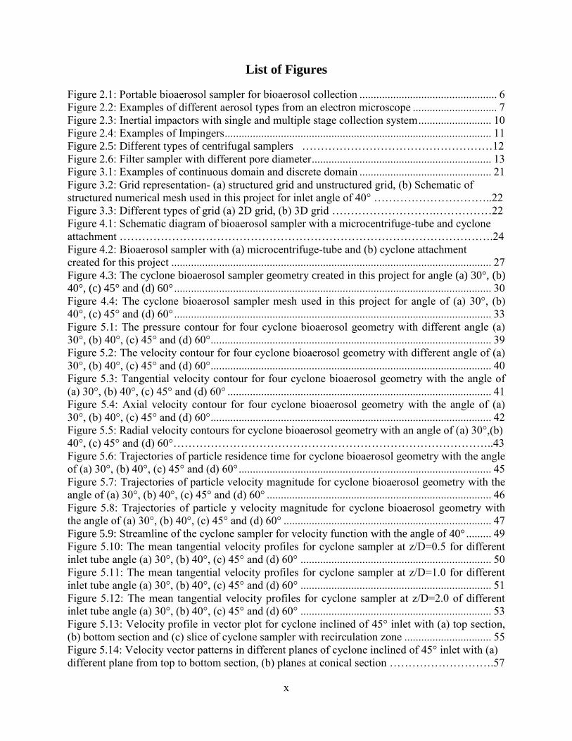
List of Figures

Figure 2.1: Portable bioaerosol sampler for bioaerosol collection ................................................. 6 Figure 2.2: Examples of different aerosol types from an electron microscope .............................. 7 Figure 2.3: Inertial impactors with single and multiple stage collection system .......................... 10 Figure 2.4: Examples of Impingers ............................................................................................... 11

Figure 2.5: Different types of centrifugal samplers ……………………………………………12

Figure 2.6: Filter sampler with different pore diameter ................................................................ 13 Figure 3.1: Examples of continuous domain and discrete domain ............................................... 21

Figure 3.2: Grid representation- (a) structured grid and unstructured grid, (b) Schematic of

structured numerical mesh used in this project for inlet angle of 40° …………………………..22

Figure 3.3: Different types of grid (a) 2D grid, (b) 3D grid ……………………….……………22

Figure 4.1: Schematic diagram of bioaerosol sampler with a microcentrifuge-tube and cyclone

attachment ……………………………………………………………………………………….24

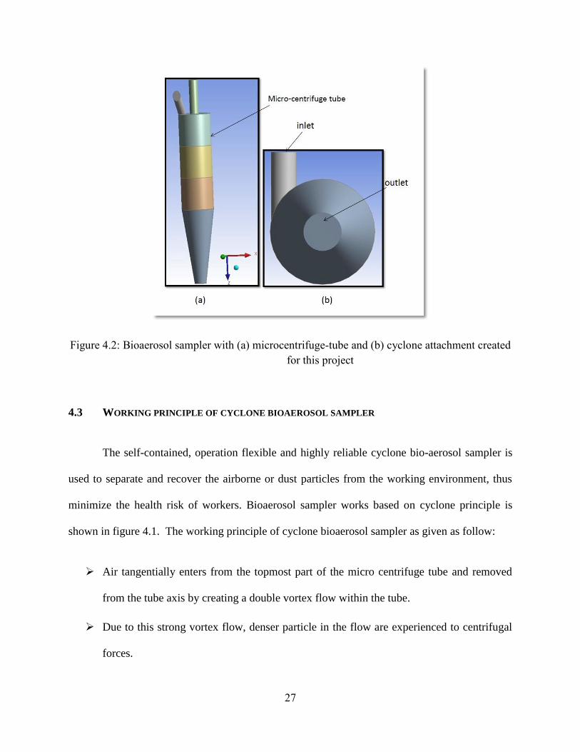
Figure 4.2: Bioaerosol sampler with (a) microcentrifuge-tube and (b) cyclone attachment created for this project .................................................................................................................. 27

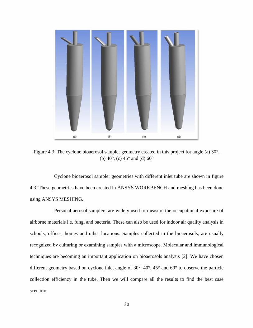
Figure 4.3: The cyclone bioaerosol sampler geometry created in this project for angle (a) 30°, (b)

40°, (c) 45° and (d) 60° ................................................................................................................. 30

Figure 4.4: The cyclone bioaerosol sampler mesh used in this project for angle of (a) 30°, (b)

40°, (c) 45° and (d) 60° ................................................................................................................. 33 Figure 5.1: The pressure contour for four cyclone bioaerosol geometry with different angle (a)

30°, (b) 40°, (c) 45° and (d) 60° .................................................................................................... 39 Figure 5.2: The velocity contour for four cyclone bioaerosol geometry with different angle of (a)

30°, (b) 40°, (c) 45° and (d) 60° .................................................................................................... 40 Figure 5.3: Tangential velocity contour for four cyclone bioaerosol geometry with the angle of

(a) 30°, (b) 40°, (c) 45° and (d) 60° .............................................................................................. 41

Figure 5.4: Axial velocity contour for four cyclone bioaerosol geometry with the angle of (a)

30°, (b) 40°, (c) 45° and (d) 60° .................................................................................................... 42

Figure 5.5: Radial velocity contours for cyclone bioaerosol geometry with an angle of (a) 30°,(b)

40°, (c) 45° and (d) 60°…………………………………………………………………………..43

Figure 5.6: Trajectories of particle residence time for cyclone bioaerosol geometry with the angle

of (a) 30°, (b) 40°, (c) 45° and (d) 60° .......................................................................................... 45

Figure 5.7: Trajectories of particle velocity magnitude for cyclone bioaerosol geometry with the

angle of (a) 30°, (b) 40°, (c) 45° and (d) 60° ................................................................................ 46 Figure 5.8: Trajectories of particle y velocity magnitude for cyclone bioaerosol geometry with

the angle of (a) 30°, (b) 40°, (c) 45° and (d) 60° .......................................................................... 47

Figure 5.9: Streamline of the cyclone sampler for velocity function with the angle of 40° ......... 49 Figure 5.10: The mean tangential velocity profiles for cyclone sampler at z/D=0.5 for different

inlet tube angle (a) 30°, (b) 40°, (c) 45° and (d) 60° .................................................................... 50

Figure 5.11: The mean tangential velocity profiles for cyclone sampler at z/D=1.0 for different

inlet tube angle (a) 30°, (b) 40°, (c) 45° and (d) 60° .................................................................... 51 Figure 5.12: The mean tangential velocity profiles for cyclone sampler at z/D=2.0 of different

inlet tube angle (a) 30°, (b) 40°, (c) 45° and (d) 60° .................................................................... 53

Figure 5.13: Velocity profile in vector plot for cyclone inclined of 45° inlet with (a) top section,

(b) bottom section and (c) slice of cyclone sampler with recirculation zone ............................... 55

Figure 5.14: Velocity vector patterns in different planes of cyclone inclined of 45° inlet with (a)

different plane from top to bottom section, (b) planes at conical section ……………………….57

xi

Figure 5.15: Collection efficiency curve with the particle diameter at flow rate of Q= 4 L/min for

cyclone sampler of different inlet tube angle (a) 30°, (b) 40°, (c) 45° and (d) 60° ...................... 58

1

Chapter 1: Introduction

This thesis is categorized into six sections. In this chapter, a brief description of the

cyclone-based bioaerosol sampler will be discussed in detail. This chapter will focus on the

significance of the bio-aerosol sampler and the process for accomplishing the research.

1.1 OVERVIEW

Cyclone-based bioaerosol samplers are extensively used in hospitals, schools, offices,

industries and agronomical poultry farms to maintain indoor and outdoor air quality, as the air

quality may degrade due to various microbial agents. These microbial agents may cause several

health issues like allergic reactions, toxic effects, and infectious diseases [1]. Due to minimal

operational costs, relatively simple geometry, and absence of moving parts and high reliability,

cyclones are widely used in industries. Bioaerosol samplers are used to separate and recover the

airborne or dust particles from the working environments such as schools, office, hospitals and

industries. This study is focused on the microbial agent fungi. A high moisture level is favorable

for fungal growth. Fungal spores are also acknowledged for asthma risk factor in indoor

environments.

Airborne particles have been characterized and detected by the use of bioaerosol samplers

from a long time. The main purpose of monitoring aerosol particles is to evaluate the social,

economic and environmental impacts on human lives and health which occurs due to respiratory

inhalation from aerosol particulates. One conventional method is used to detect and quantify

fungal aerosols and airborne particles; this is the so-called short-term area grab samples. A

considerable number of researchers have promoted techniques for detecting specific or “total”

indoor fungal species [1, 2]. The effect of change on the cyclone dimensions are varied with the

2

change of the inlet angle or the change of the cyclone cone dimension and body diameter. Thus,

researchers have developed a bioaerosol sampler that permits sample analysis without the

requirement for a sample transfer step. As a big difference from industrial cyclone samplers, the

bio-aerosol samplers do not require high temperature, high pressure loadings, so it is highly

effective to collect airborne aerosol particles/droplets including various microbial species and

airborne microorganisms. These type of bio-aerosol samplers can be directly used to supplement

CFD simulation of airborne particles transport [1, 3]. The major concern of a personal sampler is

its collection efficiency at indoor conditions for different particle/droplet size.

Though the cyclone-based bioaerosol sampler has a simple geometrical design, the

underlying mechanism that describes the position and velocity of particles and the interaction

with fluid flow in a cyclone sampler is very intricate due to intense turbulence, dynamic

anisotropy and three dimensional natures of flow [4]. The cyclone-based bioaerosol sampler

performance is measured by its collection efficiency and also by the pressure drop. In our study,

the pressure-drop is a less critical parameter than the industrial sampler. It becomes more clear

that the inlet angle, inner wall of the collection tube and the cone geometry will play critical role

for particle motions and therefore, for the collection efficiency of the sampler [1]. The effect of

change on the cyclone dimensions are varied with the change of the inlet angle or the change of

the other dimensions, such as inlet diameter, height of cylindrical and conical part. An inlet

angle in cyclone sampler is vital for cyclone performances, as it allows the collected particles to

enter the cyclone and deliver them to the discharge point of the cyclone. Though the

understanding of the physics of the flow field inside the cyclone has been advanced rather

quickly, the mathematical modelling of particle removal is not comprehensible yet [5]. The

geometry was created by using the ANSYS WORKBENCH, and the numerical simulation was

done by FLUENT 13.0.0.

3

1.2 OBJECTIVES OF THE RESEARCH

The goal of this study is to evaluate several design options, such as inlet tube angles and

different surface roughness of the collection tube inner wall through computational fluid

dynamics (CFD) simulations. CFD modeling of the change of vortex core region as well as

several velocity fluctuation profiles will shed light on the fundamental mechanism that

influences the collection efficiency. Based on the results obtained from the simulation, the best

design option will be determined.

To accomplish the project goals, the following objectives have been established:

Generate detailed data about continuous phase flow in samplers using the state-of-the art

CFD tools.

Predict the motion of the dispersed phase particles inside a bio-aerosol cyclone sample

using a 3D dispersed parcel method (DPM).

Analyze the development and evolution of the vortex core region in the sampler.

Assess the collection efficiency of the cyclone sampler by combining continuous phase

flow and dispersed phase particles.

Four cyclone geometries have been used with different inlet tube angles in this research

project. After measuring the cyclone-based bioaerosol sampler’s collection efficiency, the best

design option will be selected. The roughest inner wall proceeds to the best collection efficiency.

The best collection efficiency leads to choose the best bioaerosol cyclone sampler design.

Cyclone performances may be enhanced by the change of inlet tube angle.

4

1.3 THESIS OUTLOOK

This thesis is divided into six chapters. Chapter 1 outlines the importance of cyclone bio-

aerosol samplers and the procedure for achieving the research in shortly. It also depicts the goals

and objectives of this study that was designed to accomplish the result. Chapter 2 features the

literature review on bioaerosol sampler, different types of bioaerosol and technologies to capture

particles from working environments, which links the background to this research. Chapter 3

focuses on the theory behind the calculation and gives information for software outline. Chapter

4 gives a comprehensive description of experimental methods and boundary conditions under

which the simulations were performed. It includes the geometry creation, mesh analysis and

other conditions that are used to perform the simulation. A discussion of the numerical results

and theoretical calculations are discussed in Chapter 5. Finally, chapter 6 summarizes the

conclusion about this work as well as recommendations for future work.

The numerical analysis was done by using the commercial software ANSYS FLUENT

13.0.0 and ANSYS CFX. These CFD tools are available on multicore processor computers at the

cSETR Computational Lab, The University of Texas at El Paso.

5

Chapter 2: Literature Review

Chapter 2 features the literature review of a cyclone-based bioaerosol sampler, different

types, source and size of micro-organisms that may be removed from the personal sampler. It

also discusses the various types of bioaerosol samplers used in sampling of bioaerosol particles,

and their uses will be explained in greater detail later.

2.1 CYCLONE BIOAEROSOL SAMPLER

Aerosol particles are the solid or liquid particulate matters that are suspended in air or

any other gaseous environments. These aerosol particles are varied with size, shape and origin.

Bioaerosol particles are particles of biological origin that might release from living organisms

[6]. These particles are comprised of bacteria, viruses, pollen, spores and toxin; while their sizes

may vary from 0.015- 0.45 μm for viruses and 1.0-100 μm for fungal spores. Bioaerosol

sampling and characterization is complicated because of their attachment to non-viable particles

and recurrent phenomena in particle accumulation. Bioaerosol sampling includes airborne

particles collection and analysis of microorganisms within the sampler. These two

interdependent actions are governed by aerosol physics and microbiology respectively.

Dr. Bean T. Chen, an aerosol scientist from NIOSH Health Effects Lab, has developed a

new design of cyclone bioaerosol sampler while working on his research project. This cyclone

bioaerosol sampler is a flow device that cleans the air from indoor and outdoor environments by

taking the contaminated particles (i.e. bioaerosols and dust particles) from a working

environment. Several microbial agents like bioaerosol and dust particles are responsible for

various health issues which may include fatigue, allergic reactions, asthma and chronic lungs and

6

several heart diseases. Figure 2.1 shows a portable bioaerosol sampler that is used in bioaerosol

collection.

Figure 2.1: Portable bioaerosol sampler for bioaerosol collection

2.2 BIOAEROSOLS

Bioaerosols are the airborne particles that are suspended in air and have biological origin.

These particles are small in size, and their range varies from less than one micrometer (<1μm) to

one hundred micrometers (100μm). In case of outdoor air, 30 percent of all particles larger than

0.2 µm are considered to be of biological origin [7]. Different types of bioaerosol particles based

on particle size and concentration are described in following charts [8]:

Table 2.1: Bioaerosol sizes and concentrations in normal environment

Type of Bioaerosols Size (µm) Concentration (#/m3)

Viruses 0.02-0.3 -

Bacteria 0.3-10 0.5 – 1,000

Fungal Spores 0.5-30 0 – 10,000

Pollen 10-100 1 – 1,000

7

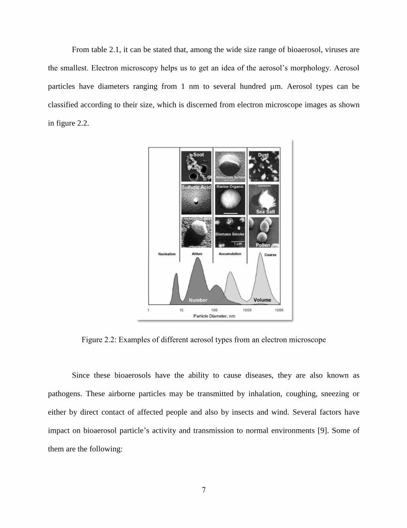
From table 2.1, it can be stated that, among the wide size range of bioaerosol, viruses are

the smallest. Electron microscopy helps us to get an idea of the aerosol’s morphology. Aerosol

particles have diameters ranging from 1 nm to several hundred µm. Aerosol types can be

classified according to their size, which is discerned from electron microscope images as shown

in figure 2.2.

Figure 2.2: Examples of different aerosol types from an electron microscope

Since these bioaerosols have the ability to cause diseases, they are also known as

pathogens. These airborne particles may be transmitted by inhalation, coughing, sneezing or

either by direct contact of affected people and also by insects and wind. Several factors have

impact on bioaerosol particle’s activity and transmission to normal environments [9]. Some of

them are the following:

8

1. Relative Humidity and Temperature- Due to the hygroscopic nature of the

bioaerosols, a particle’s permanence is affected by their dehydration or rehydration

rate. This water transfer rate is directly related to their relative humidity and

temperature.

2. Oxygen- Toxic oxygen may reduce the viability of anaerobic airborne bacteria.

Oxygen concentration also affects the survival rate of the bacteria by developing their

growth on low oxygen conditions.

3. Radiation- Radiation effects exacerbate free-radical reactions by breaking DNA

strands and protein-DNA crosslinks as well as by damaging protein, lipids, membrane

and nucleic acids. Long wave radiation has less effect on bioaerosol viability.

4. Other Pollutants: The presence of ozone in outdoor environments subdued the

survival rate of outdoor bioaerosols, which enhance airborne disease’s transmission in

indoor environments than outdoors.

2.3 BIOAEROSOL SAMPLER SELECTION

According to type and level of air sampling, commonly used and commercially available

bioaerosol samplers can be selected [9]. These samplers are subdivided based on their

mechanism of air sampling on microorganisms. A classification of the bioaerosol sampler is

shown in table 2.2 based on the mechanisms and type of sampling device [7].

9

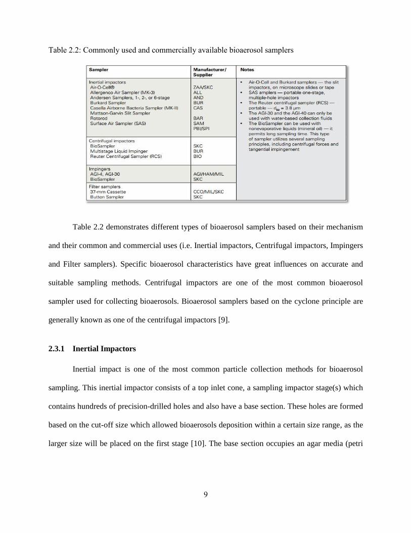
Table 2.2: Commonly used and commercially available bioaerosol samplers

Table 2.2 demonstrates different types of bioaerosol samplers based on their mechanism

and their common and commercial uses (i.e. Inertial impactors, Centrifugal impactors, Impingers

and Filter samplers). Specific bioaerosol characteristics have great influences on accurate and

suitable sampling methods. Centrifugal impactors are one of the most common bioaerosol

sampler used for collecting bioaerosols. Bioaerosol samplers based on the cyclone principle are

generally known as one of the centrifugal impactors [9].

2.3.1 Inertial Impactors

Inertial impact is one of the most common particle collection methods for bioaerosol

sampling. This inertial impactor consists of a top inlet cone, a sampling impactor stage(s) which

contains hundreds of precision-drilled holes and also have a base section. These holes are formed

based on the cut-off size which allowed bioaerosols deposition within a certain size range, as the

larger size will be placed on the first stage [10]. The base section occupies an agar media (petri

10

dish) where the accumulated air particles are deposited. Since the cut-off sizes are known for the

impactors, they can give acquainted size-dependent collection efficiencies at ease [11].

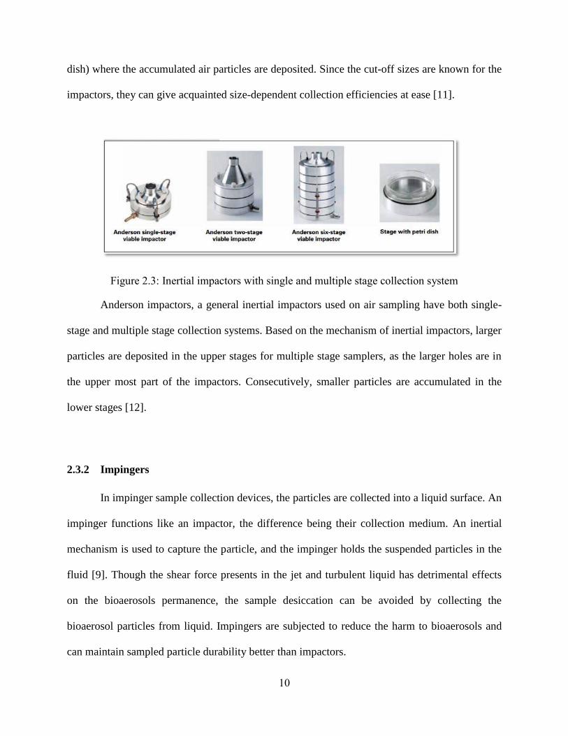
Figure 2.3: Inertial impactors with single and multiple stage collection system

Anderson impactors, a general inertial impactors used on air sampling have both single-

stage and multiple stage collection systems. Based on the mechanism of inertial impactors, larger

particles are deposited in the upper stages for multiple stage samplers, as the larger holes are in

the upper most part of the impactors. Consecutively, smaller particles are accumulated in the

lower stages [12].

2.3.2 Impingers

In impinger sample collection devices, the particles are collected into a liquid surface. An

impinger functions like an impactor, the difference being their collection medium. An inertial

mechanism is used to capture the particle, and the impinger holds the suspended particles in the

fluid [9]. Though the shear force presents in the jet and turbulent liquid has detrimental effects

on the bioaerosols permanence, the sample desiccation can be avoided by collecting the

bioaerosol particles from liquid. Impingers are subjected to reduce the harm to bioaerosols and

can maintain sampled particle durability better than impactors.

11

Figure 2.4: Examples of Impingers

Different types of impingers are shown in Figure 2.4. AGI-30 and AGI-4 are the most

conventional impingers used in bioaerosols collection. The cutoff diameter is 0.3 µm for an AGI-

30 impinger. Because of the inertia and minor flow of the sampler, particles larger than the cut-

off size are collected during sampling. Consecutively, particles smaller than 0.3 µm are subjected

to the major flow, decreasing the sampling efficiency [13]. The particle cut-off size mainly

depends on the flow rates of the sampler [14]. In case of multistage liquid impinger (MSLI),

three different sampling flow rates have been used to separate the particles into three size

fractions.

2.3.3 The Centrifugal Sampler

The Aerojet cyclone sampler and the Biotest RCS centrifugal are the most conventional

centrifugal samplers used for air sampling. Cyclones have been worked as a pre-sampler before

the impactors and filters from a long time [15]. These samplers work based on the centrifugal

force effects by spinning the bioaerosol particles throughout the tube axis. Larger particle are

subjected to fall at the bottom of the sampler due to their inertia, while the smaller ones escape

12

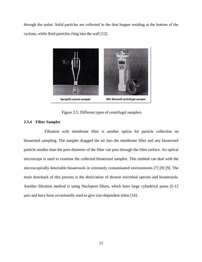
through the outlet. Solid particles are collected in the dust hopper residing at the bottom of the

cyclone, while fluid particles cling into the wall [12].

Figure 2.5: Different types of centrifugal samplers

2.3.4 Filter Sampler

Filtration with membrane filter is another option for particle collection on

bioaerosol sampling. The sampler dragged the air into the membrane filter and any bioaerosol

particle smaller than the pore diameter of the filter can pass through the filter surface. An optical

microscope is used to examine the collected bioaerosol samples. This method can deal with the

microscopically detectable bioaerosols in extremely contaminated environments [7] [8] [9]. The

main drawback of this process is the desiccation of diverse microbial species and bioaerosols.

Another filtration method is using Nuclepore filters, which have large cylindrical pores (5-12

μm) and have been occasionally used to give size-dependent inlets [16].

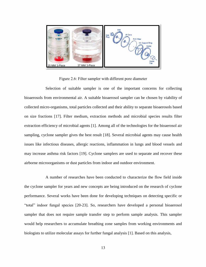
13

Figure 2.6: Filter sampler with different pore diameter

Selection of suitable sampler is one of the important concerns for collecting

bioaerosols from environmental air. A suitable bioaerosol sampler can be chosen by viability of

collected micro-organisms, total particles collected and their ability to separate bioaerosols based

on size fractions [17]. Filter medium, extraction methods and microbial species results filter

extraction efficiency of microbial agents [1]. Among all of the technologies for the bioaerosol air

sampling, cyclone sampler gives the best result [18]. Several microbial agents may cause health

issues like infectious diseases, allergic reactions, inflammation in lungs and blood vessels and

may increase asthma risk factors [19]. Cyclone samplers are used to separate and recover these

airborne microorganisms or dust particles from indoor and outdoor environment.

A number of researches have been conducted to characterize the flow field inside

the cyclone sampler for years and new concepts are being introduced on the research of cyclone

performance. Several works have been done for developing techniques on detecting specific or

“total” indoor fungal species [20-23]. So, researchers have developed a personal bioaerosol

sampler that does not require sample transfer step to perform sample analysis. This sampler

would help researchers to accumulate breathing zone samples from working environments and

biologists to utilize molecular assays for further fungal analysis [1]. Based on this analysis,

14

public health specialists can apply and improve control strategies on improving air quality for

indoor and outdoor environments.

15

Chapter 3: Numerical Method

The numerical analysis of fluid flow gives us an extensive idea of the computational fluid

dynamics (CFD), which becomes a great concern to engineers and scientists. CFD owes its

popularity for predicting fluid flow, heat transfer, and chemical species transport in different

environmental condition analysis [24]. With the advent of powerful parallel computers and

advancement of computational techniques in recent years, CFD gives quantitative and qualitative

analysis of fluid flow that is able to deal with the real life problems with better accuracy [25].

In this numerical analysis-based work, we have discussed several cases for different inlet

angles with different geometry of the cyclone sampler and the particle collection efficiency of

this device. To get the best collection efficiency, we have made a comparison of all obtained

results from different cyclone geometry. It would take a huge cost to check all these cases in

practical life. Therefore, numerical analysis provides a guideline to choose the best experimental

setup to make it more cost effective [5].

3.1 GOVERNING EQUATIONS

The flow field inside the cyclone sampler is a complex phenomenon in fluid dynamics

problem. A combined approach on CFD and discrete element method (DEM) is exhibited on this

project which explains the particle-particle and particle-fluid interactions [26-37]. For better

understanding of complex particle-fluid flow, CFD–DEM approach has been extended in several

studies on the gas–solid flow of a gas cyclone [38-42]. CFD analyzes the fluid dynamic

phenomena by using numerical methods. Fluid Dynamics (FD) solution can be obtained by sets

of governing equation. Navier–Stokes equation controlled the gas phase simulation in CFD–

DEM modelling [43]. The Navier–Stokes equations are nonlinear partial differential equations

16

that illustrates the conservation of linear momentum for a linearly viscous (Newtonian),

incompressible fluid flow [44, 45]. Density does not vary with the fluid motion in an

incompressible flow.

3.1.1 Mathematical modelling:

Computational fluid dynamics (CFD) method is used to model the performance of cyclone

bioaerosol sampler and it can anticipate the flow field characteristics and the particle trajectories

inside the cyclone. The intricate swirling turbulent flow in a cyclone places great demands on

the numerical techniques and the turbulence models employed in the CFD codes when modelling

the collection performance.

FLUENT uses a finite volume method (FVM) to solve the governing equations. Reynolds-

averaged Navier-Stokes equations (RANS) for steady and incompressible fluid flow can be

expressed as:

𝜌𝑢𝑗𝜕𝑢𝑖

𝜕𝑥𝑗= −

𝜕𝑝

𝜕𝑥𝑖+

𝜕

𝜕𝑥𝑗[𝜇 (

𝜕𝑢𝑖

𝜕𝑥𝑗+𝜕𝑢𝑗

𝜕𝑥𝑖)] +

𝜕𝜏𝑖𝑗

𝜕𝑥𝑗 (3.1)

𝜕𝑢𝑖

𝜕𝑥𝑖= 0 (3.2)

where, the superscripts i, j = 1, 2 represent the Cartesian coordinate system components,

𝜌, 𝑢, 𝑝 𝑎𝑛𝑑 μ is the fluid density, velocity, pressure and viscosity respectively and

𝜏𝑖𝑗 = −𝜌𝑢𝑖́ 𝑢�́� (3.3)

which is defined as the Reynolds stress tensor that indicates the turbulent fluctuations effects

on the fluid flow. The dash and overbar represent the fluctuating part and a Reynolds average

term.

17

Reynolds stress model

The standard k-ɛ model is inappropriate due to its certain limitations in the case of strong

swirling flow [46]. Reynolds stress model (RSM) can solve the transport equations of Reynolds

stress model within particular stress components and improves the isotropic turbulence of k- ɛ

model. The transport equations of Reynolds stress (RSM) model can be written as follows:

𝜕𝜌𝑢𝑖𝑢𝑗

𝜕𝑡+

𝜕

𝜕𝑥𝑘 (𝑈𝑘𝜕𝜌𝑢𝑖𝑢𝑗) =

𝑃𝑖𝑗 + ∅𝑖𝑗 +𝜕

𝜕𝑥𝑘 [(𝜇 +

2

3 𝑐𝑠 𝜌

𝑘2

ɛ )𝜕𝜌𝑢𝑖𝑢𝑗

𝜕𝑥𝑘 ] −

2

3𝛿𝑖𝑗휀𝜌 (3.4)

where, k is the turbulent kinetic energy, ɛ is the dissipation rate of k, pressure-strain correlation

is expressed in ∅𝑖𝑗 terms and 𝑃𝑖𝑗 is the production term of 𝑢𝑖𝑢𝑗 which can be written as follows:

P = -ρ (𝑢. 𝑢(∇𝑈)𝑇 + (∇ 𝑈) (3.5)

The turbulent dissipation rate presents within the individual stress equations. The equation for

the turbulent dissipation rate ɛ is given as:

𝜕𝜌𝜀

𝜕𝑡+ ∇. (ρ Uε) =

𝜀

𝑘(𝑐𝜀1𝑃 − 𝑐𝜀2) + ∇. [

1

𝜎𝜀𝑅𝑆(𝜇 + 𝜌𝐶𝜇𝑅𝑆

𝑘2

𝜀) . 휀]

(3.6)

The model constants in these equations are

𝑐𝑠 = 0.22; 𝑐𝜀1 = 1.45; 𝑐𝜀2 = 1.9; 𝑐𝜇𝑅𝑆 = 0.115

18

Model Equations for Particle Motion

The equation of dispersed particles motion can be by integrating the force balance equation

in a Lagrangian reference frame. FLUENT anticipates the trajectory of a discrete phase in a

Lagrangian reference frame [47]. The force balance equation of a single dispersed particle can

be written (for the x direction in Cartesian coordinates) as

𝑑𝑢𝑝

𝑑𝑡= 𝐹d (u - up)

𝑔𝑥 (𝜌𝑝 – 𝜌)

𝜌𝑝+ Fx (3.7)

where, Fx is an additional acceleration term , u is the fluid phase velocity, up is the particle

velocity, 𝜌p is the density of the particle, 𝑔𝑥 is the gravitational acceleration and Fd (u-up) is the

drag force per unit particle mass where Fd can be written as [49]:

𝐹𝐷 =18𝜇

𝜌𝑝𝑑𝑝2 𝐶𝑑

24 𝑅𝑒 (3.8)

Here, 𝜇 is the molecular viscosity of the fluid, 𝜌 is the fluid density, dp is the particle

diameter and drag coefficient Cd can be determined by Morsi and Alexander’s correlation. Re is

the relative Reynolds number, which is defined as,

Re = 𝜌 𝑑𝑝|𝑢𝑝−𝑢|

𝜇 (3.9)

Saffman’s Lift Force

The Saffman's lift force (lift due to shear) can also be included in coupled force term. The

Saffman lift force is a generalization form from Li and Ahmadi which can be written as:

�⃗� = 2𝐾𝑣1/2𝜌𝑑𝑖𝑗

𝜌𝑝𝑑𝑝(𝑑𝑙𝑘𝑑𝑘𝑙)1/4 (�⃗� − �⃗�𝑝) (3.10)

19

where K = 2:594 and dij is the deformation tensor. This form of the lift force is intended for small

particle Reynolds numbers.

3.2 BOUNDARY CONDITIONS

Boundary conditions (BC) are a set of conditions that specify the flow and thermal

variables at the boundary of its domain. These are verily important parameter for the

mathematical model and FLUENT simulations [48]. Without appropriate boundary condition

settings, numerical simulation would not be able to solve the flow analysis. CFD requires proper

boundary condition on the outer and inner surfaces of the fluid domain, while the inner surfaces

represent fluid-structure interfaces. In general, boundary conditions are two types i.e.

i. Dirichlet boundary conditions – specify the value of the variable at the

boundary, e.g. 𝑢( ) = 𝑐 𝑛 𝑎𝑛

ii. Neumann boundary conditions – specify the gradient normal to the boundary of

the variable at the boundary, e.g. 𝜕 𝑢( ) = 𝑐 𝑛 𝑎𝑛

Usually boundary conditions depend on the type of analysis (incompressible or compressible).

Another type of boundary condition is used to analyze fluid dynamics problem is called mixed

type boundary conditions. These types of boundary condition specify a function of the form

𝑎𝑢( ) + 𝜕 𝑢( ) = 𝑐 𝑛 𝑎𝑛 at the boundary.

Proper boundary conditions give an accurate solution of numerical simulation. Boundary

conditions used at each face of each computational domain. It specifies physical conditions (e.g.

solid wall, symmetry plane, etc.) in the boundary region and interfaces between contiguous or

20

overlapped domain [49]. Inaccurate boundary condition settings can lead to a nonphysical

simulation results. Therefore, defining proper and effective boundary condition is the most

important part of CFD analysis.

For this research, we have used four different boundary conditions, i.e., velocity inlet at inlet,

outflow at outlet, wall for boundary wall and interior BC for the interior zone.

i. Velocity inlet: Velocity inlet BC defines the velocity vectors and scalar properties of the

flow at flow inlets. Since the total (or stagnation) properties of the flow are not fixed,

their values may vary to give the recommended velocity distribution.

ii. Outflow: Outflow BC is used when flow velocity and pressure are not known previously.

It can’t be used in unsteady compressible flow and where the backflow occurs. Other

flow variables are extrapolated from the interior.

iii. Wall: Wall BC is used to bound fluid and solid regions. No-slip BC is implemented on

the wall in viscous flow. Based on flow field details inside the computational domain, the

shear stress and heat transfer between the fluid and the wall are calculated.

iv. Interior: Interior BC is used on flow fluid through an area.

3.3 GRID GENERATION

Grid is generated in ANSYS WORKBENCE software for the CFD solver. Discrete

domain with grid can replace the continuous domain for CFD simulation. In continuous domain,

each flow function can be outlined at every point of the domain. On the other side, each flow

function is defined at the grid points only in discrete domain. The discrete system is a set of

coupled, algebraic equations in the discrete variables. Discrete system includes a very large

number of iterative calculations which is done by the digital computer. Figure 3.1 shows the

21

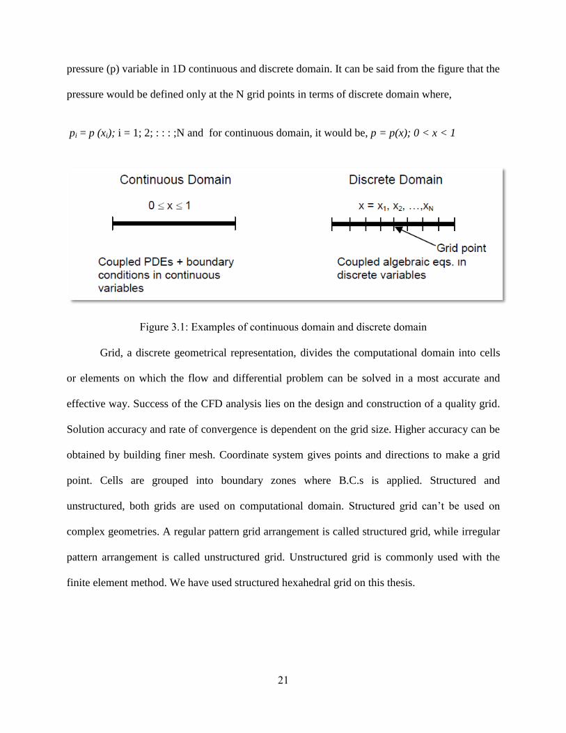
pressure (p) variable in 1D continuous and discrete domain. It can be said from the figure that the

pressure would be defined only at the N grid points in terms of discrete domain where,

pi = p (xi); i = 1; 2; : : : ;N and for continuous domain, it would be, p = p(x); 0 < x < 1

Figure 3.1: Examples of continuous domain and discrete domain

Grid, a discrete geometrical representation, divides the computational domain into cells

or elements on which the flow and differential problem can be solved in a most accurate and

effective way. Success of the CFD analysis lies on the design and construction of a quality grid.

Solution accuracy and rate of convergence is dependent on the grid size. Higher accuracy can be

obtained by building finer mesh. Coordinate system gives points and directions to make a grid

point. Cells are grouped into boundary zones where B.C.s is applied. Structured and

unstructured, both grids are used on computational domain. Structured grid can’t be used on

complex geometries. A regular pattern grid arrangement is called structured grid, while irregular

pattern arrangement is called unstructured grid. Unstructured grid is commonly used with the

finite element method. We have used structured hexahedral grid on this thesis.

22

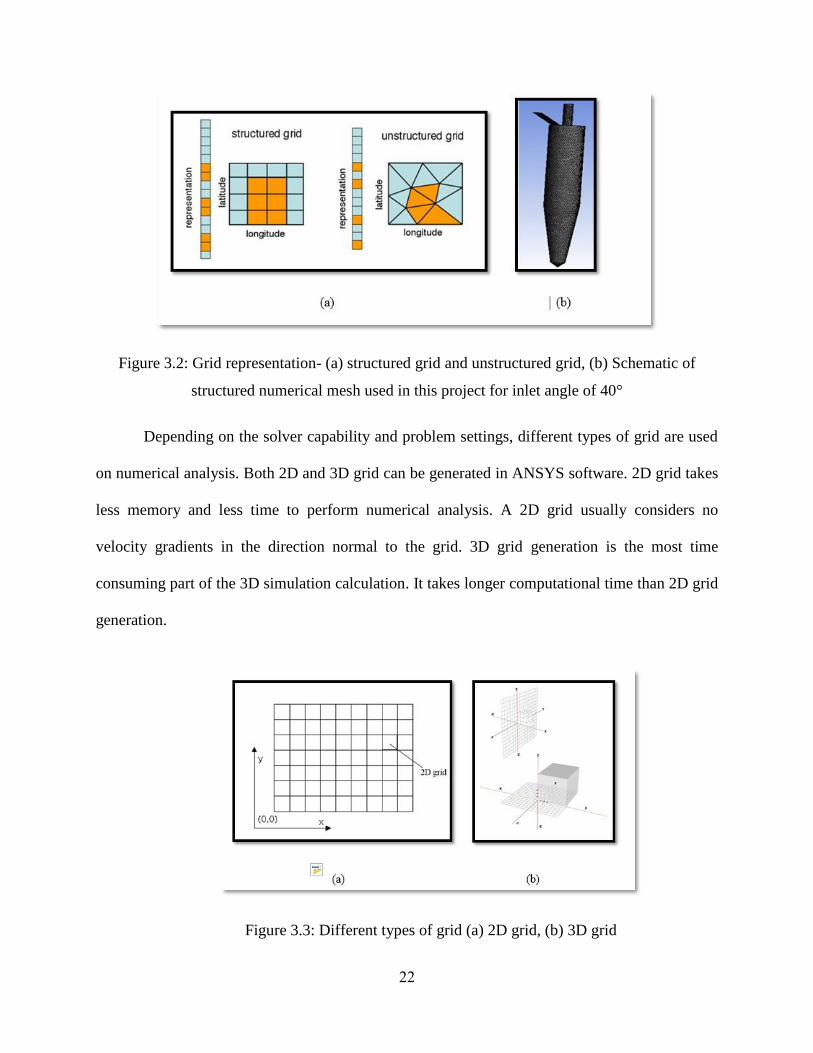
Figure 3.2: Grid representation- (a) structured grid and unstructured grid, (b) Schematic of

structured numerical mesh used in this project for inlet angle of 40°

Depending on the solver capability and problem settings, different types of grid are used

on numerical analysis. Both 2D and 3D grid can be generated in ANSYS software. 2D grid takes

less memory and less time to perform numerical analysis. A 2D grid usually considers no

velocity gradients in the direction normal to the grid. 3D grid generation is the most time

consuming part of the 3D simulation calculation. It takes longer computational time than 2D grid

generation.

Figure 3.3: Different types of grid (a) 2D grid, (b) 3D grid

23

Governing equations are not good enough to get analytical solutions of fluid flow or heat

transfer problem. Finite volume method can solve the partial differential equations on fluid flow

analysis. To analyze fluid flow inside a computational domain, the domain is discretized into

smaller volumes or subdomains. Then the governing equations solve every discretized volume.

These discretized subdomains are called elements or cells and the set of all elements are called

mesh. Appropriate choice of mesh will impede the simulation error and can give us an accurate

result during the flow analysis in Fluent.

24

Chapter 4: Methodology of Cyclone Sampler Simulation

In this chapter the theory behind the numerical analysis of the collection efficiency of a

cyclone-based bioaerosol sampler will be elaborately explained. At first, design and working

principle of bioaerosol sampler will be discussed. Then four geometries with different inlet tube

angle will be shown. At last the collection efficiency will be characterized for different cyclone

geometry will be obtained from several equations.

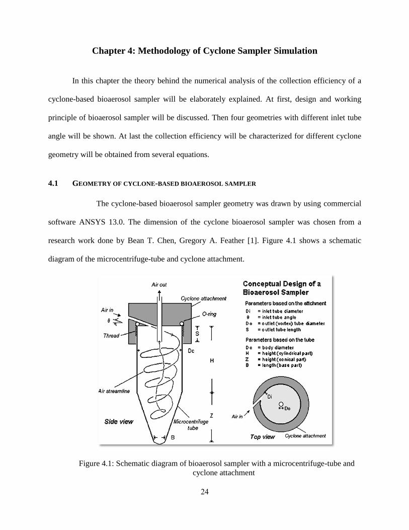
4.1 GEOMETRY OF CYCLONE-BASED BIOAEROSOL SAMPLER

The cyclone-based bioaerosol sampler geometry was drawn by using commercial

software ANSYS 13.0. The dimension of the cyclone bioaerosol sampler was chosen from a

research work done by Bean T. Chen, Gregory A. Feather [1]. Figure 4.1 shows a schematic

diagram of the microcentrifuge-tube and cyclone attachment.

Figure 4.1: Schematic diagram of bioaerosol sampler with a microcentrifuge-tube and

cyclone attachment

25

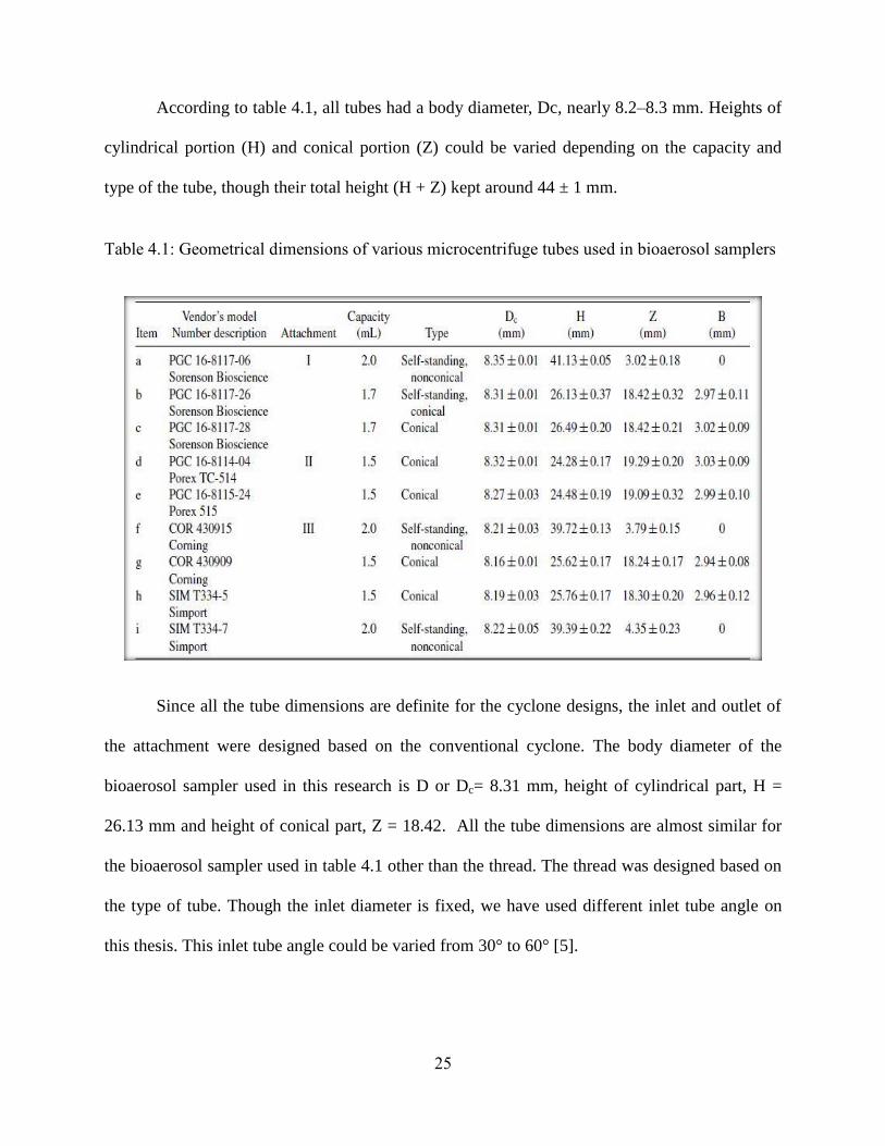
According to table 4.1, all tubes had a body diameter, Dc, nearly 8.2–8.3 mm. Heights of

cylindrical portion (H) and conical portion (Z) could be varied depending on the capacity and

type of the tube, though their total height (H + Z) kept around 44 ± 1 mm.

Table 4.1: Geometrical dimensions of various microcentrifuge tubes used in bioaerosol samplers

Since all the tube dimensions are definite for the cyclone designs, the inlet and outlet of

the attachment were designed based on the conventional cyclone. The body diameter of the

bioaerosol sampler used in this research is D or Dc= 8.31 mm, height of cylindrical part, H =

26.13 mm and height of conical part, Z = 18.42. All the tube dimensions are almost similar for

the bioaerosol sampler used in table 4.1 other than the thread. The thread was designed based on

the type of tube. Though the inlet diameter is fixed, we have used different inlet tube angle on

this thesis. This inlet tube angle could be varied from 30° to 60° [5].

26

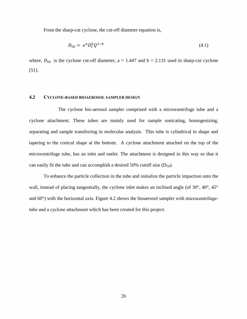
From the sharp-cut cyclone, the cut-off diameter equation is,

= 𝑒 1 (4.1)

where, is the cyclone cut-off diameter, a = 1.447 and b = 2.131 used in sharp-cut cyclone

[51].

4.2 CYCLONE-BASED BIOAEROSOL SAMPLER DESIGN

The cyclone bio-aerosol sampler comprised with a microcentrifuge tube and a

cyclone attachment. These tubes are mainly used for sample sonicating, homogenizing,

separating and sample transferring in molecular analysis. This tube is cylindrical in shape and

tapering to the conical shape at the bottom. A cyclone attachment attached on the top of the

microcentrifuge tube, has an inlet and outlet. The attachment is designed in this way so that it

can easily fit the tube and can accomplish a desired 50% cutoff size (D50).

To enhance the particle collection in the tube and initialize the particle impaction onto the

wall, instead of placing tangentially, the cyclone inlet makes an inclined angle (of 30°, 40°, 45°

and 60°) with the horizontal axis. Figure 4.2 shows the bioaerosol sampler with microcentrifuge-

tube and a cyclone attachment which has been created for this project.

27

Figure 4.2: Bioaerosol sampler with (a) microcentrifuge-tube and (b) cyclone attachment created

for this project

4.3 WORKING PRINCIPLE OF CYCLONE BIOAEROSOL SAMPLER

The self-contained, operation flexible and highly reliable cyclone bio-aerosol sampler is

used to separate and recover the airborne or dust particles from the working environment, thus

minimize the health risk of workers. Bioaerosol sampler works based on cyclone principle is

shown in figure 4.1. The working principle of cyclone bioaerosol sampler as given as follow:

Air tangentially enters from the topmost part of the micro centrifuge tube and removed

from the tube axis by creating a double vortex flow within the tube.

Due to this strong vortex flow, denser particle in the flow are experienced to centrifugal

forces.

28

Particles which have sufficient inertia have an impact on the tube walls.

Some of the particles are retained on the walls and due to the secondary flow in the

boundary layers; other particles migrate to the bottom of the tube.

The vortex flow headway to the bottom of the cyclone sampler that reduces the rotational

radius of the stream thus separates smaller particles from main flow.

Two types of vortices formed inside the cyclone- inner vortex and outer vortex. Outer

vortex spirals downward from the inlet along the cyclone wall towards the bottom end

and inner vortex starts from the cone apex then spirals upward to the outlet.

The purpose of this cyclone-based bioaerosol sampler design is to collect more particles

in the microcentrifuge tube, which could be used as the collection receptacle for further

analysis.

Cyclone attachment placed on the top of the microcentrifuge tube is used to get a desired

50% cutoff size (D50).

Cyclone inlet makes an inclined angle with the horizontal axis to enhance the particle

collection in the tube within specific size range and initialize the particle impaction onto

the wall.

4.4 PROBLEM DESCRIPTION OF CYCLONE-BASED BIOAEROSOL SAMPLER

The present study deals with the cyclone-based bioaerosol sampler as shown in

figure 4.1. The geometrical dimensions of four cyclone sampler used in this study are given in

table 4.2. All of their dimensions are the same only the inlet tube angle is different for the four

cyclone sampler. From figure 4.1, it is seen that the inlet angle of air sucking into the sample is

denoted by θ, different angle will directly impact the tangential and axial velocity components.

The inlet section is changed by using 30°, 40°, 45° and 60° with respect to the microcentrifuge

29

tube. All the cases will be simulated by using different inlet tube angle on the flow field of

cyclone sampler and overall collection efficiencies will be measured.

Table 4.2: Geometric configuration of Cyclone studied for this project

Dimension Size(mm)

Body diameter, D or Dc 8.31

Gas outlet diameter, Do 2.24

Gas inlet diameter, Di 1.99

Outlet tube length, S 2.91

Height of cylindrical part, H 26.13

Height of conical part, Z 18.42

Length of Base, B 2.97

Table 4.3 shows the different inlet tube angle used in this study. We have created

four cyclone samplers with different inlet tube angle to observe the difference of flow pattern

and particle collection efficiency.

Table 4.3: Geometrical inlet tube angle of cyclone studied

Dimension Angle ( ° )

Inlet tube angle, θ 40°

30°

45°

60°

In this research, we have used a 3D full order high-fidelity CFD tool angle to

simulate the particle flow inside a bio-aerosol cyclone sampler to evaluate different design

options for optimization of the collection efficiency of particles.

30

Figure 4.3: The cyclone bioaerosol sampler geometry created in this project for angle (a) 30°,

(b) 40°, (c) 45° and (d) 60°

Cyclone bioaerosol sampler geometries with different inlet tube are shown in figure

4.3. These geometries have been created in ANSYS WORKBENCH and meshing has been done

using ANSYS MESHING.

Personal aerosol samplers are widely used to measure the occupational exposure of

airborne materials i.e. fungi and bacteria. These can also be used for indoor air quality analysis in

schools, offices, homes and other locations. Samples collected in the bioaerosols, are usually

recognized by culturing or examining samples with a microscope. Molecular and immunological

techniques are becoming an important application on bioaerosols analysis [2]. We have chosen

different geometry based on cyclone inlet angle of 30°, 40°, 45° and 60° to observe the particle

collection efficiency in the tube. Then we will compare all the results to find the best case

scenario.

31

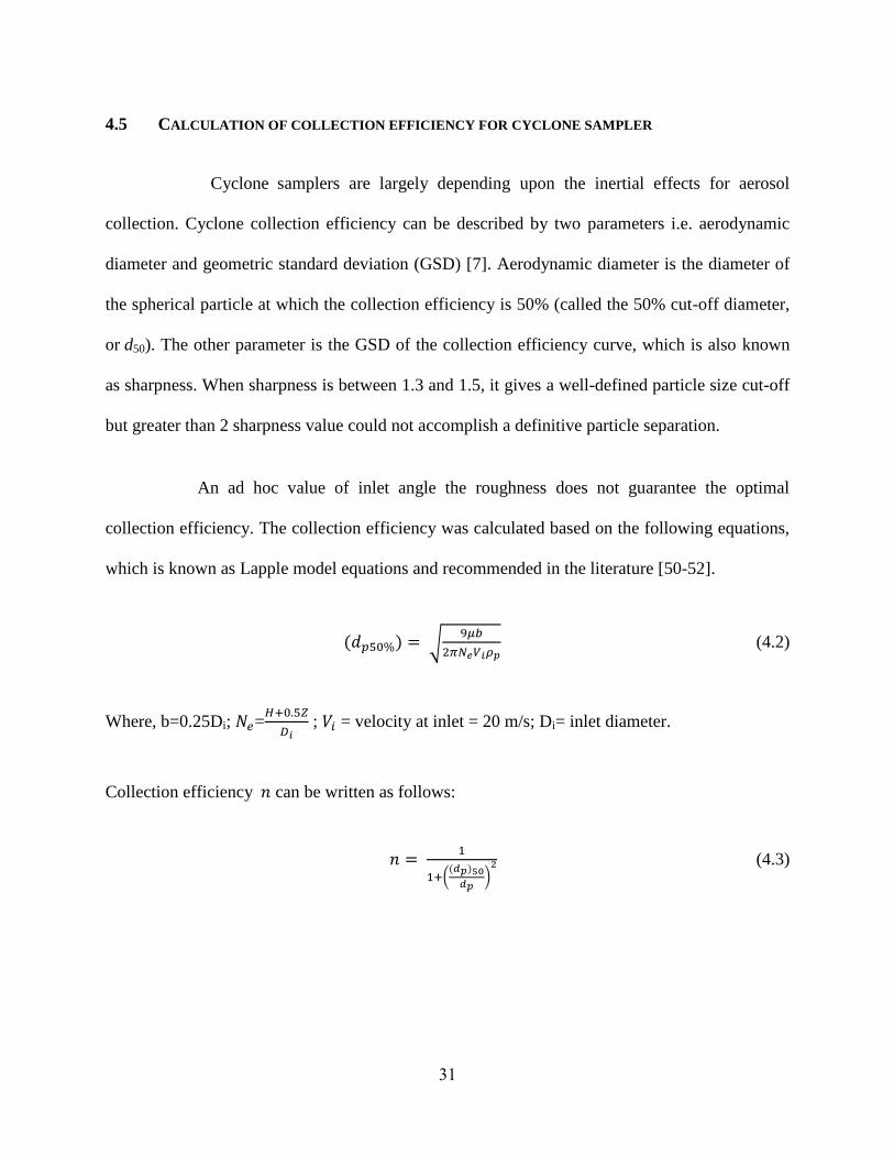
4.5 CALCULATION OF COLLECTION EFFICIENCY FOR CYCLONE SAMPLER

Cyclone samplers are largely depending upon the inertial effects for aerosol

collection. Cyclone collection efficiency can be described by two parameters i.e. aerodynamic

diameter and geometric standard deviation (GSD) [7]. Aerodynamic diameter is the diameter of

the spherical particle at which the collection efficiency is 50% (called the 50% cut-off diameter,

or d50). The other parameter is the GSD of the collection efficiency curve, which is also known

as sharpness. When sharpness is between 1.3 and 1.5, it gives a well-defined particle size cut-off

but greater than 2 sharpness value could not accomplish a definitive particle separation.

An ad hoc value of inlet angle the roughness does not guarantee the optimal

collection efficiency. The collection efficiency was calculated based on the following equations,

which is known as Lapple model equations and recommended in the literature [50-52].

(𝑑𝑝 ) = √ 𝜇

2 𝑖𝜌𝑝 (4.2)

Where, b=0.25Di; = .

𝐷𝑖 ; 𝑖 = velocity at inlet = 20 m/s; Di= inlet diameter.

Collection efficiency 𝑛 can be written as follows:

𝑛 = 1

1 ((𝑑𝑝)

𝑑𝑝)2 (4.3)

32

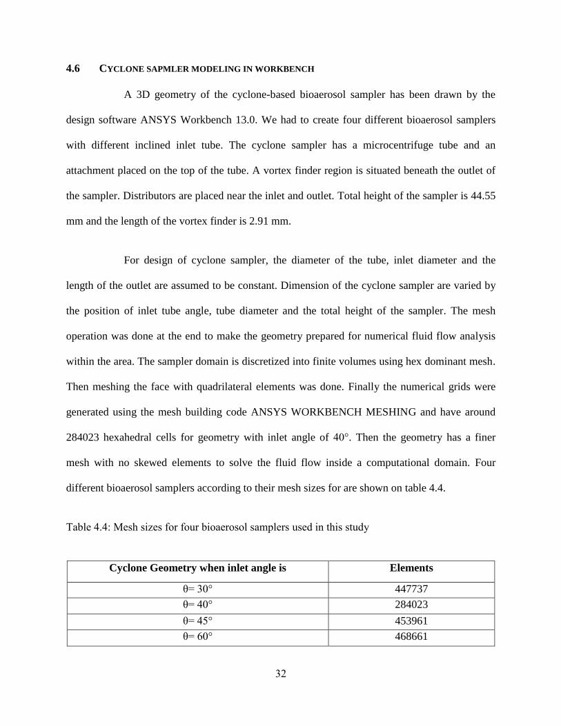
4.6 CYCLONE SAPMLER MODELING IN WORKBENCH

A 3D geometry of the cyclone-based bioaerosol sampler has been drawn by the

design software ANSYS Workbench 13.0. We had to create four different bioaerosol samplers

with different inclined inlet tube. The cyclone sampler has a microcentrifuge tube and an

attachment placed on the top of the tube. A vortex finder region is situated beneath the outlet of

the sampler. Distributors are placed near the inlet and outlet. Total height of the sampler is 44.55

mm and the length of the vortex finder is 2.91 mm.

For design of cyclone sampler, the diameter of the tube, inlet diameter and the

length of the outlet are assumed to be constant. Dimension of the cyclone sampler are varied by

the position of inlet tube angle, tube diameter and the total height of the sampler. The mesh

operation was done at the end to make the geometry prepared for numerical fluid flow analysis

within the area. The sampler domain is discretized into finite volumes using hex dominant mesh.

Then meshing the face with quadrilateral elements was done. Finally the numerical grids were

generated using the mesh building code ANSYS WORKBENCH MESHING and have around

284023 hexahedral cells for geometry with inlet angle of 40°. Then the geometry has a finer

mesh with no skewed elements to solve the fluid flow inside a computational domain. Four

different bioaerosol samplers according to their mesh sizes for are shown on table 4.4.

Table 4.4: Mesh sizes for four bioaerosol samplers used in this study

Cyclone Geometry when inlet angle is Elements

θ= 30° 447737

θ= 40° 284023

θ= 45° 453961

θ= 60° 468661

33

Figure 4.4: The cyclone bioaerosol sampler mesh used in this project for angle of (a) 30°,

(b) 40°, (c) 45° and (d) 60°

Computational grids used in this project have 447737 and 284023 cells for inlet tube

angle of 30° and 40° respectively. The other mesh used in this study for four bioaerosol samplers

are shown through table 4.4 and later on figure 4.4.

34

4.7 CFD SIMULATION OF CYCLONE SAPMLER

A commercially available CFD code, FLUENT is used to solve the discretized

equations (conservation of mass, momentum and energy equations) by finite volume

formulation. Once the bioaerosol sampler modeling had done, boundary condition was

implemented. In this study, a velocity inlet boundary condition was applied at inlet; outflow BC

at outlet and no slip BC at the walls. Air was considered as continuous phase material and water-

liquid as a dispersed phase material in this study. The Eulerian-Lagrangian approach has been

employed to simulate the cyclone sampler. Numerical simulations were done by the Eulerian

reference frame for continuous gas phase flow and by Lagrangian method for dispersed phase

particle trajectories. 3-D, unsteady and incompressible fluid flow in Eulerian formulation was

introduced in this investigation. The Lagrangian approach resolves the transport equations of

continuous phase in Eulerian frame and then integrates the dispersed phase equations by

tracking individual spherical particles through the converged flow field. The stochastic Particle

Tracking Model outlined the particle motions by tracking particle trajectories in Lagrangian

frame of reference. By keeping track on the number of particles escaping through the outflow,

the collection efficiency could be measured.

There are a lot of turbulence model available in FLUENT solver. As k-ɛ model has

some limitations to swirling turbulent flow, Reynolds stress turbulence model (RSTM) was used

to simulate the cyclone-based bioaerosol sampler. The standard wall function is chosen for the

near-wall treatment. Because of the small size (i.e. 0.5-16 μm) of the injected particle in the

sampler, the velocity fluctuation of the small particles on turbulent dispersion cannot be

overlooked. The fluctuating gas velocities can be determined by using a discrete random walk

(DRW) model which is based on the stochastic tracking scheme.

35

The SIMPLEC (Semi-Implicit Method for Pressure-Linked Equations-Consistent) scheme

for pressure – velocity coupling has been used in finite volume method to discretize the partial

differential equations and second order upwind scheme is used in the solution method for the

control volume variables. The inlet velocity is considered as 20 m/s for this study [4]. The

maximum number of integration steps were 5 × 10 and a length scale of 0.005m were chosen

for the dispersed particle trajectories. Particle time step size of 0.001s with an automated tracking

scheme was selected for the numerical experiments and an accuracy of 10 was performed for

accuracy control. In inlet, the turbulent intensity was set as 0.1 and Reynolds stresses are

specified as normal and shear stresses which is 666.67 m2/s

2 and 0 respectively.

4.8 NUMERICAL MODELING

A highly reliable CFD modeling can help us to understand the physics inside the flow

field of cyclone sampler. Appropriate computational modeling is essential to comprehend the

flow physics of the system and determine the underlying methodology of CFD. It can accurately

predict the behavior of flow with the help of powerful digital computers. The numerical solution

of computational flow modeling includes resolving the fluid dynamics phenomena in details.

Grid refinement is important to determine the ordered discretization error in CFD simulation.

Computational problem size can be augmented by grid refinement which will increase the need

for parallel computing. The multiphase flow considered here is isothermal system which does not

involve temperature change, even though temperature variation could play a role to change the

deposition of particle inside the tube. The flow is 3D incompressible gas-droplet/particle two-

phase interactions.

36

Problem with mathematical modelling of flow field includes for indoor air measurement,

the inlet air velocity is large enough that the flow is turbulent in the sampler. Turbulence models

are based on statistical analysis as it is becoming an interesting alternative on CFD modelling. In

past years, different turbulent models, e.g. standard − model, − model, and −

have been applied to RANS to model cyclone flow inside the sampler [53]. Large disparate

results compared to experimental data have been reported in published literature (e.g. Chen

1997). For this reason, different turbulent models have been justified for cyclone flow as a first

step of the design evaluation. On the other hand, the numerical simulation efficiency mainly

depends on the form of the turbulence modelling. As standard k–ɛ turbulence model conducts to

impracticable tangential velocities and enormous turbulent viscosities, previous studies indicate

the inability of standard k–ɛ turbulence model to simulate the highly swirling turbulence flow

[54]. Since Reynolds stress turbulence model (RSTM) justifies the stream curvature effects,

rotation and the swirling flow effects, this (RSTM) model is appropriate for highly anisotropic

flows. So, the preciseness of the numerical simulation can be improved by Reynolds stress

turbulence model (RSTM) [55-57].

We carried out CFD analysis for various design option to evaluate the particles collection

efficiency using Fluent 13.0 software. Several velocity fluctuation profiles will describe

fundamental mechanism inside the bio-aerosol cyclone sampler. Finally, the best design option

will be chosen for cyclone sampler based on their particle collection efficiency.

4.8.1 Solver Settings

Numerical analysis was performed by using a commercially available CFD code,

FLUENT 13.0 that utilizes the finite volume formulation to perform segregated or coupled

calculations with the help of conservation of mass, momentum and energy equations [50]. The

37

flow is assumed to be turbulent. We have chosen RSM in this study. Velocity distribution is

calculated by using the pressure based solver for steady-state flow. Energy equation was enabled

for this numerical analysis from the solver panel. The temperature assumed to be constant along

the velocity distribution through the cyclone sampler. Fluid properties were maintained mixing-

law for mixture-species which means that the properties such as, density, specific heat capacity,

thermal conductivity, and viscosity were composition dependent. Air and water-liquid were

considered as continuous and dispersed phase material in this study. After calculation of

continuous phase flow on Eulerian reference frame, the particle trajectories for dispersed phase

were computed through Lagrangian method. Spherical particles are used in discrete phase

modelling.

38

Chapter 5: Results & Discussion

The numerical results on the performance of cyclone-based bioaerosol sampler for

different inlet tube angle are presented in this chapter. To validate the continuous phase model,

we have used RSM for better accuracy over other models and the flow will be specified with

different velocity fluctuation profiles. Then the particle trajectories calculations for the dispersed

phase will be undertaken until the particles reach at the bottom of the sampler. We have used

Eulerian-Lagrangian approach to simulate the cyclone sampler. Four different cyclone

geometries have been studied. At last, a comparison will be made for all these four cyclone

geometries to find the best design option.

5.1 RESULTS OF CONTINUOUS PHASE SIMULATION ON CYCLONE SAMPLER

CFD is an important tool to describe the details of flow field of a cyclone sampler.

The RSM used in this study described the turbulence model and DPM described the dispersed

phase. RSM model is very effective to comprehend the flow field of cyclone sampler.

Continuous phase model validates the flow individualizations with different velocity fluctuation

profiles. RSM is used to simulate the fluid flow field inside the cyclone sampler and the fluid

flow behavior is reviewed in the terms of velocity components of the sampler.

5.1.1 Pressure field

The pressure contour plot shows that the static pressure decrease from wall to center

and due to high swirling velocity in the central region, a negative pressure region found in the

vortex finder. So, if any particle enters into this zone is supposes to escape through vortex finder

39

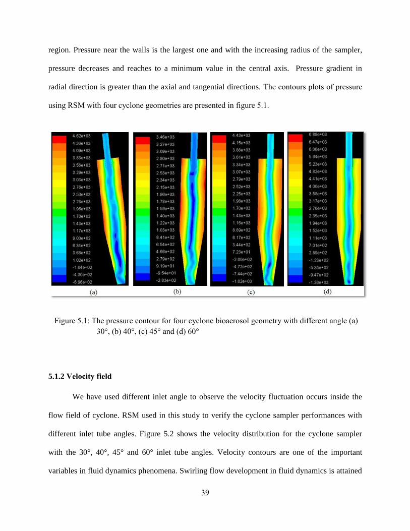
region. Pressure near the walls is the largest one and with the increasing radius of the sampler,

pressure decreases and reaches to a minimum value in the central axis. Pressure gradient in

radial direction is greater than the axial and tangential directions. The contours plots of pressure

using RSM with four cyclone geometries are presented in figure 5.1.

Figure 5.1: The pressure contour for four cyclone bioaerosol geometry with different angle (a)

30°, (b) 40°, (c) 45° and (d) 60°

5.1.2 Velocity field

We have used different inlet angle to observe the velocity fluctuation occurs inside the

flow field of cyclone. RSM used in this study to verify the cyclone sampler performances with

different inlet tube angles. Figure 5.2 shows the velocity distribution for the cyclone sampler

with the 30°, 40°, 45° and 60° inlet tube angles. Velocity contours are one of the important

variables in fluid dynamics phenomena. Swirling flow development in fluid dynamics is attained

40

by the numerical simulations in fluid dynamics. Their effects on the velocity distribution on

figure 5.2 for different inlet section angles are observed. There is recirculation occurred inside

the cyclone due to their high swirling velocity. Smaller velocity is found near the vortex finder

region. As the flow moves towards the conical section of the cyclone, the flow became

constricted due to the curtailed flow area. Therefore, the velocity increases as the particle

separation happens at the main separation area.

Figure 5.2: The velocity contour for four cyclone bioaerosol geometry with different angle of (a)

30°, (b) 40°, (c) 45° and (d) 60°

5.1.3 Tangential velocity

Tangential velocity plays an important role in three-dimensional incompressible fluid

flow of cyclone sampler because of their approach of generating centrifugal force. As the

tangential velocity is the prevalent component in the sampler, so the contours plot of the velocity

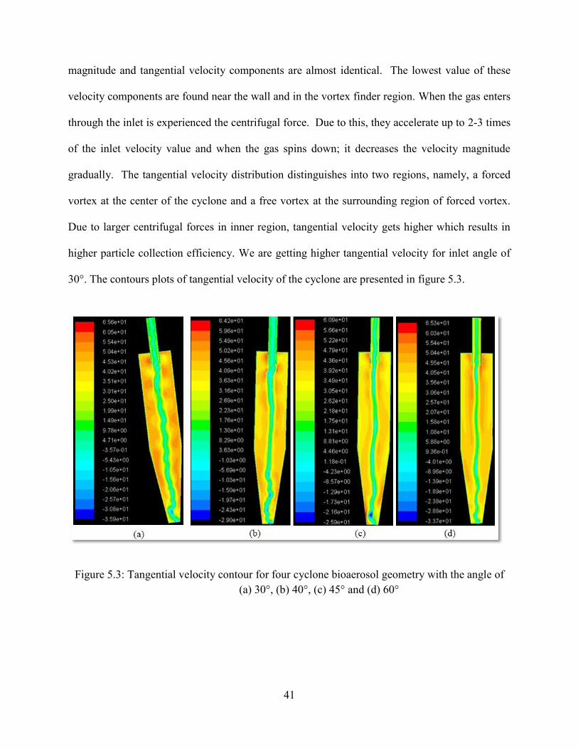
41

magnitude and tangential velocity components are almost identical. The lowest value of these

velocity components are found near the wall and in the vortex finder region. When the gas enters

through the inlet is experienced the centrifugal force. Due to this, they accelerate up to 2-3 times

of the inlet velocity value and when the gas spins down; it decreases the velocity magnitude

gradually. The tangential velocity distribution distinguishes into two regions, namely, a forced

vortex at the center of the cyclone and a free vortex at the surrounding region of forced vortex.

Due to larger centrifugal forces in inner region, tangential velocity gets higher which results in

higher particle collection efficiency. We are getting higher tangential velocity for inlet angle of

30°. The contours plots of tangential velocity of the cyclone are presented in figure 5.3.

Figure 5.3: Tangential velocity contour for four cyclone bioaerosol geometry with the angle of

(a) 30°, (b) 40°, (c) 45° and (d) 60°

42

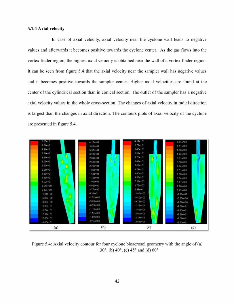
5.1.4 Axial velocity

In case of axial velocity, axial velocity near the cyclone wall leads to negative

values and afterwards it becomes positive towards the cyclone center. As the gas flows into the

vortex finder region, the highest axial velocity is obtained near the wall of a vortex finder region.

It can be seen from figure 5.4 that the axial velocity near the sampler wall has negative values

and it becomes positive towards the sampler center. Higher axial velocities are found at the

center of the cylindrical section than in conical section. The outlet of the sampler has a negative

axial velocity values in the whole cross-section. The changes of axial velocity in radial direction

is largest than the changes in axial direction. The contours plots of axial velocity of the cyclone

are presented in figure 5.4.

Figure 5.4: Axial velocity contour for four cyclone bioaerosol geometry with the angle of (a)

30°, (b) 40°, (c) 45° and (d) 60°

43

The variation of axial velocity with changing inlet tube angle is most likely the

same on near to the wall, especially in the cylindrical part of the sampler. The change of axial

velocity is more noticeable in the central section with the change of inlet angle.

5.1.5 Radial velocity

On the velocity distribution of the cyclone sampler, the radial velocity has a smaller

magnitude while tangential and axial velocities always maintain a positive value. For the

contour plot of the radial velocity, the radial velocity experienced some negative inward velocity

as the flow enters into the rotating stream of the cyclone. The radial velocity also gained positive

velocity because of the centrifugal force. Radial velocity becomes negative again around the

vortex finder region as the flow directing to the center. Contours plots of radial velocity are

shown in figure 5.5.

Figure 5.5: Radial velocity contours for cyclone bioaerosol geometry with an angle of (a) 30°,

(b) 40°, (c) 45° and (d) 60°

44

In the conical section, the radial velocity of upward flows show average magnitude and

the maximum radial velocities are close to the inlet velocity. In this section, the velocity

gradually shifts inward along the axial direction. In case of cylindrical section, the intersection

point between upward flows and downward flows is independent of the axial position.

5.2 RESULTS OF DISCRETE PHASE SIMULATION ON CYCLONE SAMPLER

Because particle phase characteristics cannot be easily described by continuum models,

Lagrangian approach is used to define the particle phase. Once the continuous phase model was

determined, the Discrete Phase Model (DPM) was used to resolve for the particles trajectories of

different range. Since all the particles being considered in this thesis were in the micron range,

their effect on the fluid during particle trajectories calculation can be neglected. The particle

motion can be expressed by differential equations in Lagrangian reference frame and

incorporated to get individual particle tracking [58]. After obtaining the dynamic behavior of the

gas phase by Eulerian approach, Lagrangian-equation for a particular moving particle is to be

solved. As particle velocity and particle trajectory are computed for each particle, this approach

is more appropriate to get the discrete motion of particles. Flow behavior is reviewed in the

terms of velocity components of the sampler.

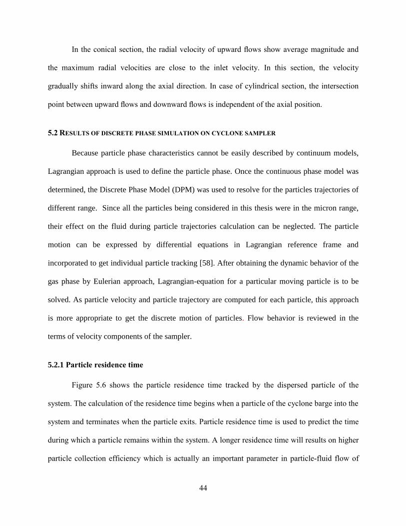
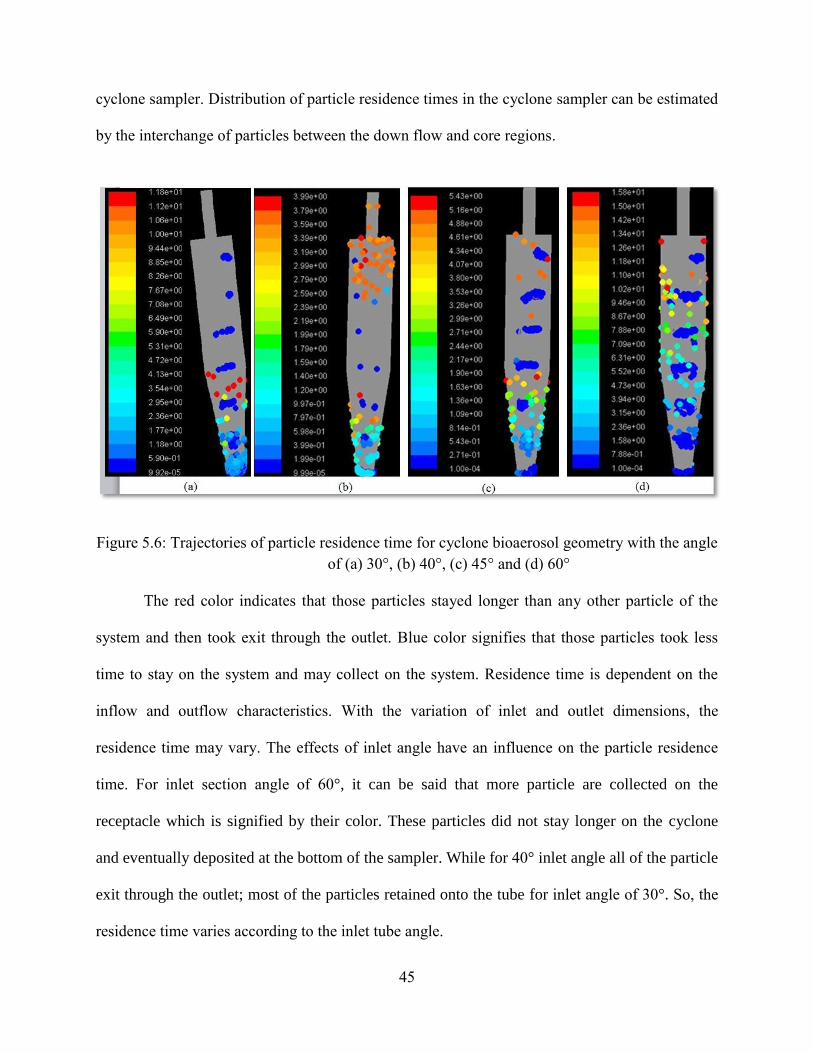
5.2.1 Particle residence time

Figure 5.6 shows the particle residence time tracked by the dispersed particle of the

system. The calculation of the residence time begins when a particle of the cyclone barge into the

system and terminates when the particle exits. Particle residence time is used to predict the time

during which a particle remains within the system. A longer residence time will results on higher

particle collection efficiency which is actually an important parameter in particle-fluid flow of

45

cyclone sampler. Distribution of particle residence times in the cyclone sampler can be estimated

by the interchange of particles between the down flow and core regions.

Figure 5.6: Trajectories of particle residence time for cyclone bioaerosol geometry with the angle

of (a) 30°, (b) 40°, (c) 45° and (d) 60°

The red color indicates that those particles stayed longer than any other particle of the

system and then took exit through the outlet. Blue color signifies that those particles took less

time to stay on the system and may collect on the system. Residence time is dependent on the

inflow and outflow characteristics. With the variation of inlet and outlet dimensions, the

residence time may vary. The effects of inlet angle have an influence on the particle residence

time. For inlet section angle of 60°, it can be said that more particle are collected on the

receptacle which is signified by their color. These particles did not stay longer on the cyclone

and eventually deposited at the bottom of the sampler. While for 40° inlet angle all of the particle

exit through the outlet; most of the particles retained onto the tube for inlet angle of 30°. So, the

residence time varies according to the inlet tube angle.

46

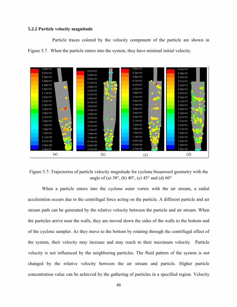
5.2.2 Particle velocity magnitude

Particle traces colored by the velocity component of the particle are shown in

Figure 5.7. When the particle enters into the system, they have minimal initial velocity.

Figure 5.7: Trajectories of particle velocity magnitude for cyclone bioaerosol geometry with the

angle of (a) 30°, (b) 40°, (c) 45° and (d) 60°

When a particle enters into the cyclone outer vortex with the air stream, a radial

acceleration occurs due to the centrifugal force acting on the particle. A different particle and air

stream path can be generated by the relative velocity between the particle and air stream. When

the particles arrive near the walls, they are moved down the sides of the walls to the bottom end

of the cyclone sampler. As they move to the bottom by rotating through the centrifugal effect of

the system, their velocity may increase and may reach to their maximum velocity. Particle

velocity is not influenced by the neighboring particles. The fluid pattern of the system is not

changed by the relative velocity between the air stream and particle. Higher particle

concentration value can be achieved by the gathering of particles in a specified region. Velocity

47

magnitude on discrete phase for cyclone sampler with four different geometry show identical

pattern.

5.2.3 Particle y velocity magnitude

Particle traces colored by the vertical velocity component of the particle are shown

in figure 5.8.

Figure 5.8: Trajectories of particle y velocity magnitude for cyclone bioaerosol geometry with

the angle of (a) 30°, (b) 40°, (c) 45° and (d) 60°

When a particle moves from one space to another, then there is a change of their vertical

velocity component. Particles moves downward near the cyclone wall and upward near the

sampler axis. This downward particle velocity near the wall causes the particle movement from

the sampler wall to the bottom of the sampler. This flow pattern is created by the double vortex

flow generation, which centrifuges the particle onto the walls. If a particle is flowed out with a

vertical velocity, it will be decelerated gradually. The vertical deceleration magnitude will be

greater, however, the greater the vertical velocity relative to the fluid. The magnitude of the

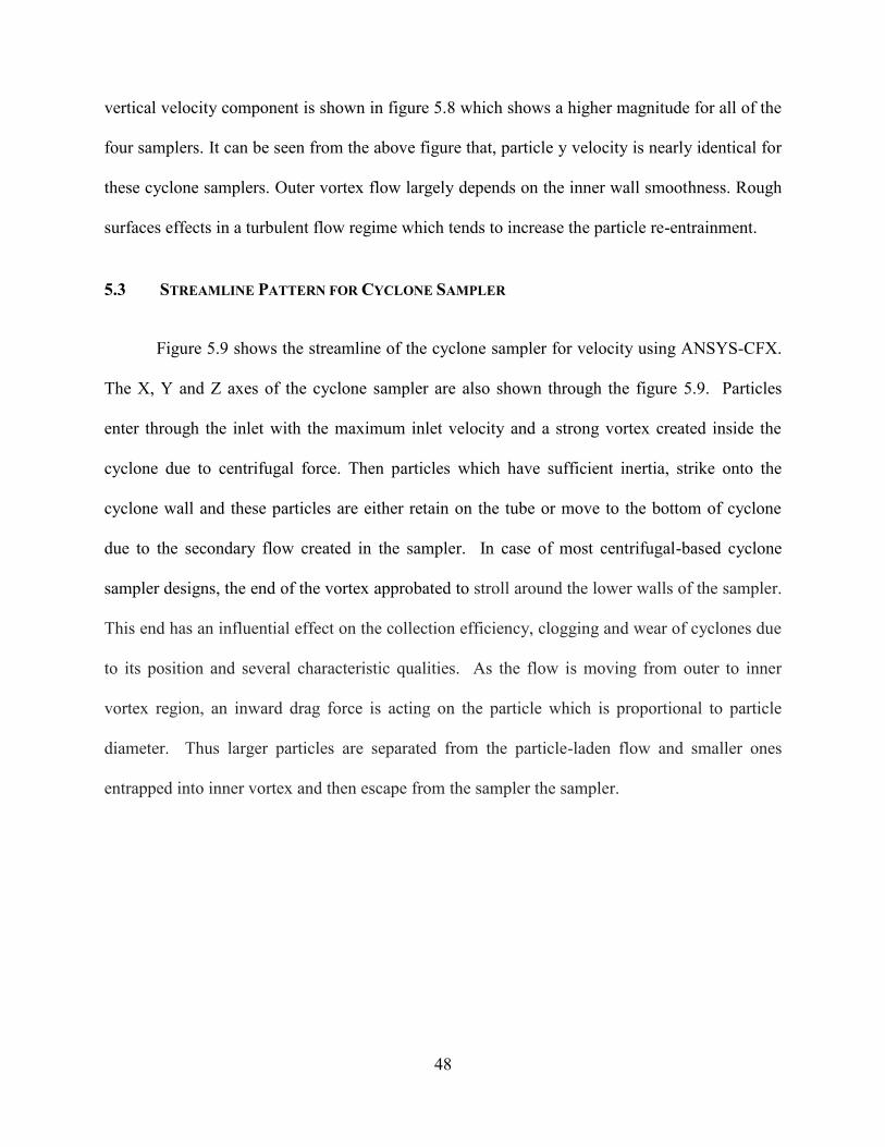
48

vertical velocity component is shown in figure 5.8 which shows a higher magnitude for all of the

four samplers. It can be seen from the above figure that, particle y velocity is nearly identical for

these cyclone samplers. Outer vortex flow largely depends on the inner wall smoothness. Rough

surfaces effects in a turbulent flow regime which tends to increase the particle re-entrainment.

5.3 STREAMLINE PATTERN FOR CYCLONE SAMPLER

Figure 5.9 shows the streamline of the cyclone sampler for velocity using ANSYS-CFX.

The X, Y and Z axes of the cyclone sampler are also shown through the figure 5.9. Particles

enter through the inlet with the maximum inlet velocity and a strong vortex created inside the

cyclone due to centrifugal force. Then particles which have sufficient inertia, strike onto the

cyclone wall and these particles are either retain on the tube or move to the bottom of cyclone

due to the secondary flow created in the sampler. In case of most centrifugal-based cyclone

sampler designs, the end of the vortex approbated to stroll around the lower walls of the sampler.

This end has an influential effect on the collection efficiency, clogging and wear of cyclones due

to its position and several characteristic qualities. As the flow is moving from outer to inner

vortex region, an inward drag force is acting on the particle which is proportional to particle

diameter. Thus larger particles are separated from the particle-laden flow and smaller ones

entrapped into inner vortex and then escape from the sampler the sampler.

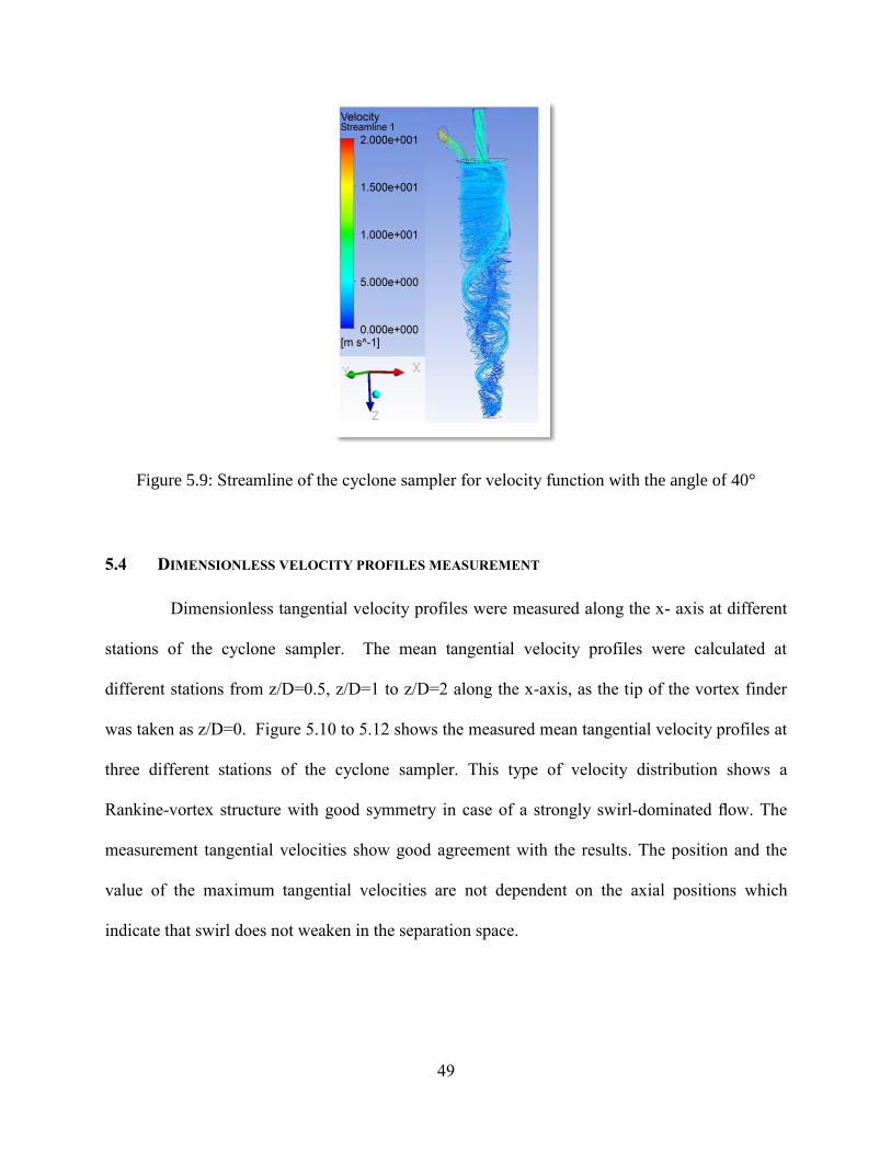
49

Figure 5.9: Streamline of the cyclone sampler for velocity function with the angle of 40°

5.4 DIMENSIONLESS VELOCITY PROFILES MEASUREMENT

Dimensionless tangential velocity profiles were measured along the x- axis at different

stations of the cyclone sampler. The mean tangential velocity profiles were calculated at

different stations from z/D=0.5, z/D=1 to z/D=2 along the x-axis, as the tip of the vortex finder

was taken as z/D=0. Figure 5.10 to 5.12 shows the measured mean tangential velocity profiles at

three different stations of the cyclone sampler. This type of velocity distribution shows a

Rankine-vortex structure with good symmetry in case of a strongly swirl-dominated flow. The

measurement tangential velocities show good agreement with the results. The position and the

value of the maximum tangential velocities are not dependent on the axial positions which

indicate that swirl does not weaken in the separation space.

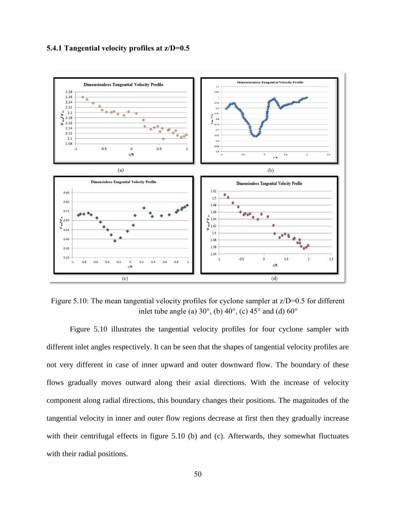
50

5.4.1 Tangential velocity profiles at z/D=0.5

Figure 5.10: The mean tangential velocity profiles for cyclone sampler at z/D=0.5 for different

inlet tube angle (a) 30°, (b) 40°, (c) 45° and (d) 60°

Figure 5.10 illustrates the tangential velocity profiles for four cyclone sampler with

different inlet angles respectively. It can be seen that the shapes of tangential velocity profiles are

not very different in case of inner upward and outer downward flow. The boundary of these

flows gradually moves outward along their axial directions. With the increase of velocity

component along radial directions, this boundary changes their positions. The magnitudes of the

tangential velocity in inner and outer flow regions decrease at first then they gradually increase

with their centrifugal effects in figure 5.10 (b) and (c). Afterwards, they somewhat fluctuates

with their radial positions.

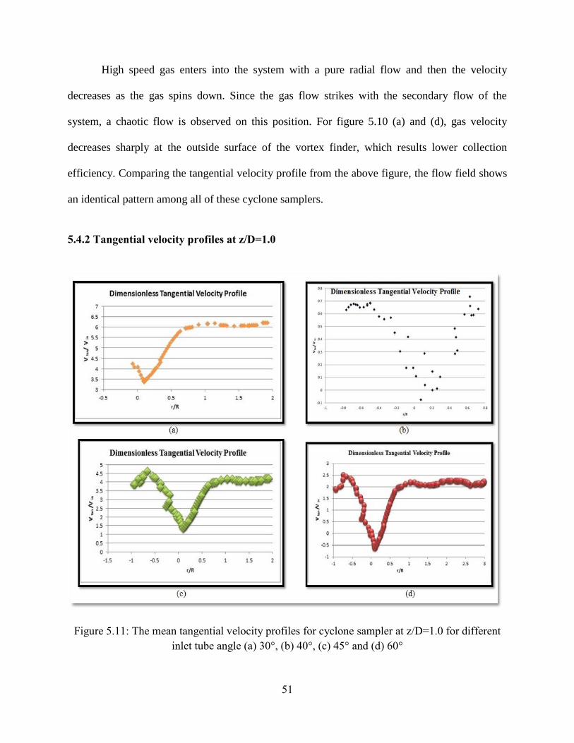
51

High speed gas enters into the system with a pure radial flow and then the velocity

decreases as the gas spins down. Since the gas flow strikes with the secondary flow of the

system, a chaotic flow is observed on this position. For figure 5.10 (a) and (d), gas velocity

decreases sharply at the outside surface of the vortex finder, which results lower collection

efficiency. Comparing the tangential velocity profile from the above figure, the flow field shows

an identical pattern among all of these cyclone samplers.

5.4.2 Tangential velocity profiles at z/D=1.0

Figure 5.11: The mean tangential velocity profiles for cyclone sampler at z/D=1.0 for different

inlet tube angle (a) 30°, (b) 40°, (c) 45° and (d) 60°

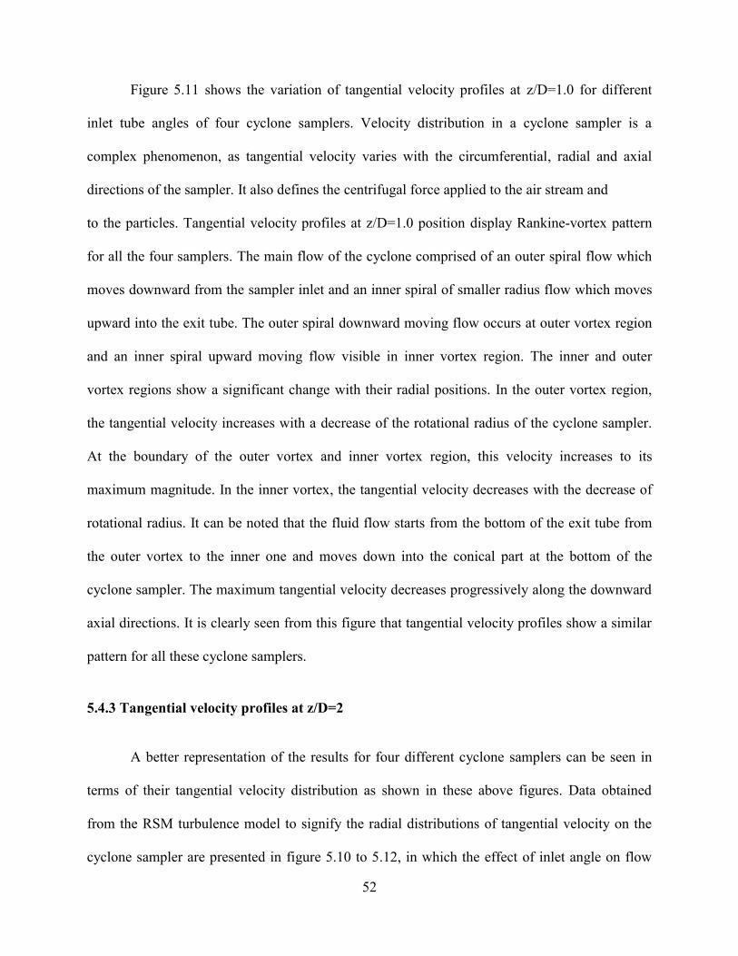
52

Figure 5.11 shows the variation of tangential velocity profiles at z/D=1.0 for different

inlet tube angles of four cyclone samplers. Velocity distribution in a cyclone sampler is a

complex phenomenon, as tangential velocity varies with the circumferential, radial and axial

directions of the sampler. It also defines the centrifugal force applied to the air stream and

to the particles. Tangential velocity profiles at z/D=1.0 position display Rankine-vortex pattern

for all the four samplers. The main flow of the cyclone comprised of an outer spiral flow which

moves downward from the sampler inlet and an inner spiral of smaller radius flow which moves

upward into the exit tube. The outer spiral downward moving flow occurs at outer vortex region

and an inner spiral upward moving flow visible in inner vortex region. The inner and outer

vortex regions show a significant change with their radial positions. In the outer vortex region,

the tangential velocity increases with a decrease of the rotational radius of the cyclone sampler.

At the boundary of the outer vortex and inner vortex region, this velocity increases to its

maximum magnitude. In the inner vortex, the tangential velocity decreases with the decrease of

rotational radius. It can be noted that the fluid flow starts from the bottom of the exit tube from

the outer vortex to the inner one and moves down into the conical part at the bottom of the

cyclone sampler. The maximum tangential velocity decreases progressively along the downward

axial directions. It is clearly seen from this figure that tangential velocity profiles show a similar

pattern for all these cyclone samplers.

5.4.3 Tangential velocity profiles at z/D=2

A better representation of the results for four different cyclone samplers can be seen in

terms of their tangential velocity distribution as shown in these above figures. Data obtained

from the RSM turbulence model to signify the radial distributions of tangential velocity on the

cyclone sampler are presented in figure 5.10 to 5.12, in which the effect of inlet angle on flow

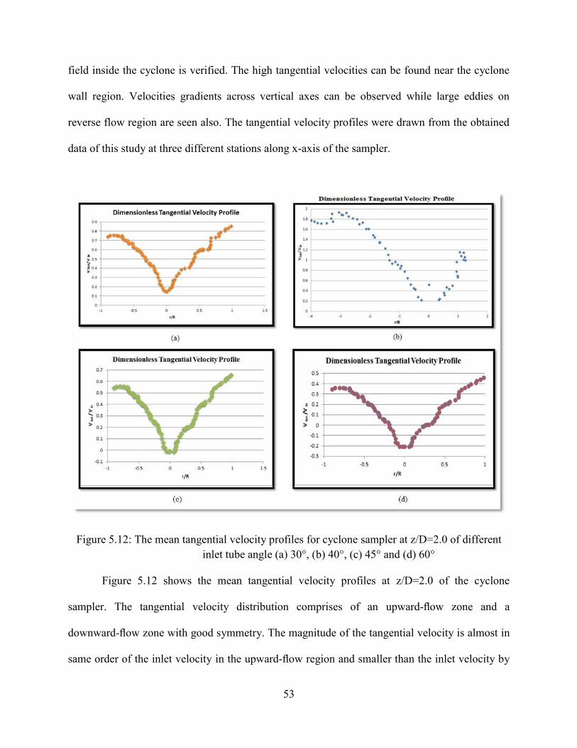
53

field inside the cyclone is verified. The high tangential velocities can be found near the cyclone

wall region. Velocities gradients across vertical axes can be observed while large eddies on

reverse flow region are seen also. The tangential velocity profiles were drawn from the obtained

data of this study at three different stations along x-axis of the sampler.

Figure 5.12: The mean tangential velocity profiles for cyclone sampler at z/D=2.0 of different

inlet tube angle (a) 30°, (b) 40°, (c) 45° and (d) 60°

Figure 5.12 shows the mean tangential velocity profiles at z/D=2.0 of the cyclone

sampler. The tangential velocity distribution comprises of an upward-flow zone and a

downward-flow zone with good symmetry. The magnitude of the tangential velocity is almost in

same order of the inlet velocity in the upward-flow region and smaller than the inlet velocity by

54

an order of magnitude in the downward-flow region. The recirculation occurs near the axis and

the inlet of the vortex finder which may results to the average pressure increment in the vortex

finder. With the increase of axial position, tangential velocity gradually shifts inward along the

axial direction and displays a cone shape.

From the above figures, it was found that with the increase of the radial position of the

sampler, the tangential velocity increases. So tangential velocity component at z/D=2 position

shows similar pattern, while velocity component at z/D=0.5 exhibits some fluctuations. It can be

seen from these figures that both the upward and the downward velocities are increasing with

inlet velocity of the sampler. Low velocities are visible in the core of the rotating flow, which is

adjacent with the center of the cyclone sampler (not in coincidence). As the distance from the

core is increasing, the velocity is accrescent to a peak value and then decreases again. For the

cyclone with 30° inlet angles have higher values than the cyclone with 60° inlet tube angle in

most cases. The tangential velocity distribution in each cross-section shows a symmetric pattern,

gradually alternates from higher to lower velocity, and then shifts towards high velocity again.

This pattern is clearly visible in all the above numerical results. High velocity fluctuation is

found near the center of the cyclone due to the advancement of the vortex core region. As the

fluid around the wall moves to underflow, the downward velocity increases consecutively. The

fluid moves then towards outlet and the upward velocity is getting increase with its radial

distance.

5.5 Velocity vectors for cyclone sampler

Velocity vector analysis for the velocity distribution is shown in the figure 5.13. Velocity

55

profile in vector plot for cyclone inclined of 45° inlet angle shows the top portion, bottom

portion and center portion of the sampler with recirculation zones respectively. Fig. 5.13 (a)

displays the top section of the cyclone sampler which shows the inlet and outlet velocity vector

of the sampler. Velocity vectors are influenced by the flow rates in the cyclone sampler. Velocity

vectors near the inlet and outlet segment exhibits the flow field in this region. Particles enter into

the sampler with a high velocity through the inlet and gradually decrease as it moves in radially

to the downward portion. Then it advances some momentum at hindmost portion of the inlet. In

Fig. 5.13 (b), Air flows in a spiral pattern from the top to the bottom of the cyclone and particles

in the flow are subjected to centrifugal forces because of the creation of a strong vortex inside

the cyclone sampler. Fig. 5.13 (c) shows the velocity vector along the center-plane which

intersects the whole cyclone sampler vertically.

Figure 5.13: Velocity profile in vector plot for cyclone inclined of 45° inlet with (a) top section,

(b) bottom section and (c) slice of cyclone sampler with recirculation zone

The velocity vector plot shows some of the minor flow patterns in the sampler flow field.

A recirculation zone appears beneath the vortex finder region, which is clearly visible at the

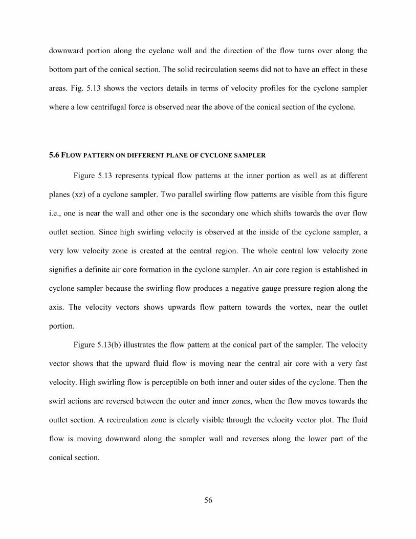
56

downward portion along the cyclone wall and the direction of the flow turns over along the

bottom part of the conical section. The solid recirculation seems did not to have an effect in these

areas. Fig. 5.13 shows the vectors details in terms of velocity profiles for the cyclone sampler

where a low centrifugal force is observed near the above of the conical section of the cyclone.

5.6 FLOW PATTERN ON DIFFERENT PLANE OF CYCLONE SAMPLER

Figure 5.13 represents typical flow patterns at the inner portion as well as at different

planes (xz) of a cyclone sampler. Two parallel swirling flow patterns are visible from this figure

i.e., one is near the wall and other one is the secondary one which shifts towards the over flow

outlet section. Since high swirling velocity is observed at the inside of the cyclone sampler, a

very low velocity zone is created at the central region. The whole central low velocity zone

signifies a definite air core formation in the cyclone sampler. An air core region is established in

cyclone sampler because the swirling flow produces a negative gauge pressure region along the

axis. The velocity vectors shows upwards flow pattern towards the vortex, near the outlet

portion.

Figure 5.13(b) illustrates the flow pattern at the conical part of the sampler. The velocity

vector shows that the upward fluid flow is moving near the central air core with a very fast

velocity. High swirling flow is perceptible on both inner and outer sides of the cyclone. Then the

swirl actions are reversed between the outer and inner zones, when the flow moves towards the

outlet section. A recirculation zone is clearly visible through the velocity vector plot. The fluid

flow is moving downward along the sampler wall and reverses along the lower part of the

conical section.

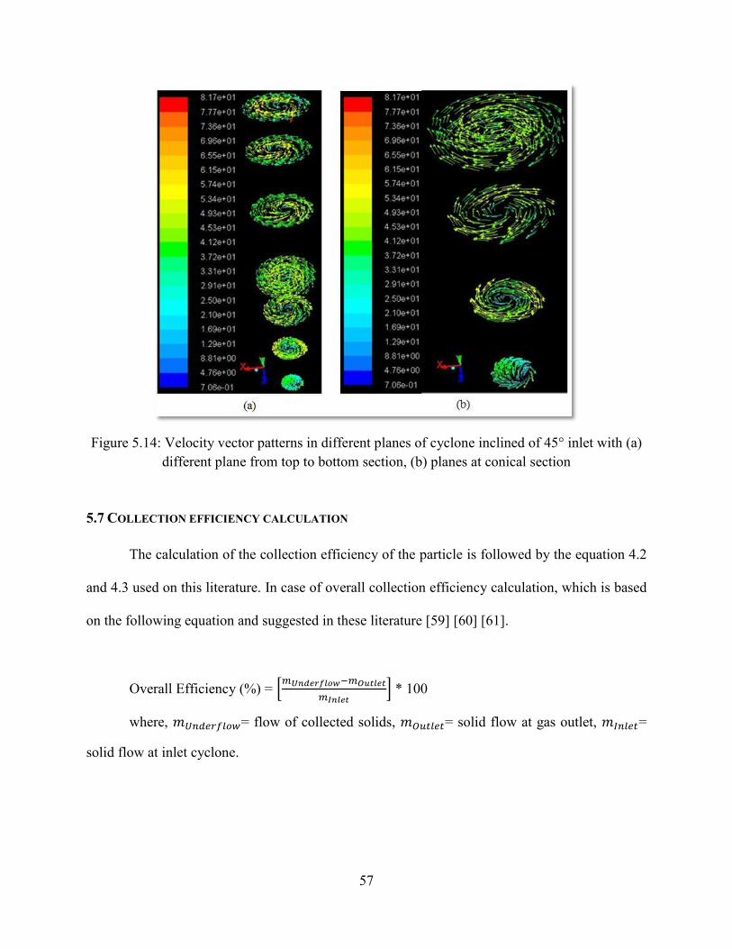
57

Figure 5.14: Velocity vector patterns in different planes of cyclone inclined of 45° inlet with (a)

different plane from top to bottom section, (b) planes at conical section

5.7 COLLECTION EFFICIENCY CALCULATION

The calculation of the collection efficiency of the particle is followed by the equation 4.2

and 4.3 used on this literature. In case of overall collection efficiency calculation, which is based

on the following equation and suggested in these literature [59] [60] [61].

Overall Efficiency (%) = [ 𝑑 𝑙 𝑢 𝑙

𝑙 ] * 100

where, 𝑑 = flow of collected solids, 𝑢𝑡 𝑡= solid flow at gas outlet, 𝑡=

solid flow at inlet cyclone.

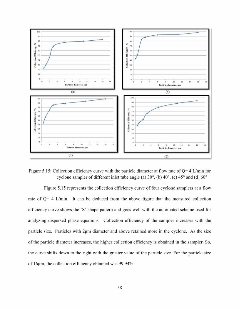
58

Figure 5.15: Collection efficiency curve with the particle diameter at flow rate of Q= 4 L/min for

cyclone sampler of different inlet tube angle (a) 30°, (b) 40°, (c) 45° and (d) 60°

Figure 5.15 represents the collection efficiency curve of four cyclone samplers at a flow

rate of Q= 4 L/min. It can be deduced from the above figure that the measured collection

efficiency curve shows the ‘S’ shape pattern and goes well with the automated scheme used for

analyzing dispersed phase equations. Collection efficiency of the sampler increases with the

particle size. Particles with 2μm diameter and above retained more in the cyclone. As the size

of the particle diameter increases, the higher collection efficiency is obtained in the sampler. So,

the curve shifts down to the right with the greater value of the particle size. For the particle size

of 16μm, the collection efficiency obtained was 99.94%.

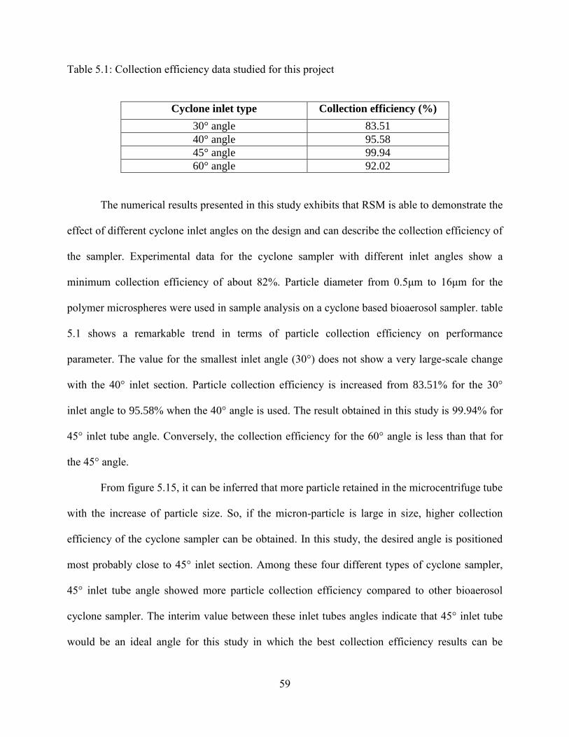
59

Table 5.1: Collection efficiency data studied for this project

Cyclone inlet type Collection efficiency (%)

30° angle 83.51

40° angle 95.58

45° angle 99.94

60° angle 92.02

The numerical results presented in this study exhibits that RSM is able to demonstrate the

effect of different cyclone inlet angles on the design and can describe the collection efficiency of

the sampler. Experimental data for the cyclone sampler with different inlet angles show a

minimum collection efficiency of about 82%. Particle diameter from 0.5μm to 16μm for the

polymer microspheres were used in sample analysis on a cyclone based bioaerosol sampler. table

5.1 shows a remarkable trend in terms of particle collection efficiency on performance

parameter. The value for the smallest inlet angle (30°) does not show a very large-scale change

with the 40° inlet section. Particle collection efficiency is increased from 83.51% for the 30°

inlet angle to 95.58% when the 40° angle is used. The result obtained in this study is 99.94% for

45° inlet tube angle. Conversely, the collection efficiency for the 60° angle is less than that for

the 45° angle.

From figure 5.15, it can be inferred that more particle retained in the microcentrifuge tube

with the increase of particle size. So, if the micron-particle is large in size, higher collection

efficiency of the cyclone sampler can be obtained. In this study, the desired angle is positioned

most probably close to 45° inlet section. Among these four different types of cyclone sampler,

45° inlet tube angle showed more particle collection efficiency compared to other bioaerosol

cyclone sampler. The interim value between these inlet tubes angles indicate that 45° inlet tube

would be an ideal angle for this study in which the best collection efficiency results can be

60

obtained. Therefore, it can be recommended from this study that changing scroll inlet angle is an

expedient way to improve cyclone sampler performance.

61

Chapter 6: Conclusion

We applied 3D full order high-fidelity CFD tool simulate particle motion and particle-air

interaction in a personal bio-aerosol sampler. Four cyclone sampler of different inlet tube angle

have been simulated using the Reynolds stress model (RSM), to observe the effect on cyclone

performance and flow pattern. FLUENT 13.0 were used to accomplish the Computational Fluid

Dynamics analysis. The inlet angles of the cyclone sampler have an impact on particle entrance

which affects cyclone efficiency in a statistically effective way. Changing the inlet tube angle

makes a considerable change in cyclone sampler performances. This study recommends a new

personal cyclone sampler design by using 30°, 40°, 45°and 60° angles for the inlet section.

Several fluid dynamics profiles and performance parameter were investigated, presented and

discussed. The fluid flow of the cyclone sampler has been characterized with different inlet angle

and flow velocity with corresponding velocity fluctuation profiles of axial, radial and tangential

components, which highlight the influence of wall boundary later on particle deposits on the

collection tube. The RSM exhibits a significant representation of fluid flow and fluid–particle

turbulent swirling flow behavior in cyclone sampler with the help of CFD technique. In order to

comprehend the sampler inlet tube angle effects on its collection efficiency based on the fluid

dynamics phenomena, elaborative flow field description was achieved through CFD simulation.

New characteristics of velocity distribution and particle tracks were obtained by application of

the RSM and DPM. Performance parameter such as collection efficiency indicates that this

different inlet angle application can give an alternative way to improve sampler performance.

Numerical results show that the inlet angle of 45 leads to a better collection efficiency

which is 99.94% where the inlet velocity and collection tube surface roughness were kept same

for different inlet tube angle. For the same inlet angle, the roughest inner wall leads to the best

62

collection efficiency. We have not done with the numerical analysis of two-stage cyclone

microcentrifuge tube sampler for the size segregated sample collection yet. We have plans in

future to perform numerical simulation on a two-stage cyclone sampler to observe the particle

collection ability of the sampler by using the current CFD techniques.

63

References

1. Chen, B.T., et al., Development of a personal sampler for collecting fungal spores.

Aerosol science and technology, 2004. 38(9): p. 926-937.

2. Lindsley, W.G., D. Schmechel, and B.T. Chen, A two-stage cyclone using

microcentrifuge tubes for personal bioaerosol sampling. Journal of Environmental

Monitoring, 2006. 8(11): p. 1136-1142.

3. Redrow, J., et al., Modeling the evaporation and dispersion of airborne sputum droplets

expelled from a human cough. Building and Environment, 2011. 46(10): p. 2042-2051.

4. Shukla, S.K., P. Shukla, and P. Ghosh, Evaluation of numerical schemes for dispersed

phase modeling of cyclone separators. Engineering Applications of Computational Fluid

Mechanics, 2011. 5(2): p. 235-246.

5. Bernardo, S., et al., 3-D computational fluid dynamics for gas and gas-particle flows in a

cyclone with different inlet section angles. Powder Technology, 2006. 162(3): p. 190-200.

6. Ksiazek, T.G., et al., A novel coronavirus associated with severe acute respiratory

syndrome. New England Journal of Medicine, 2003. 348(20): p. 1953-1966.

7. Kulkarni, P., P.A. Baron, and K. Willeke, Aerosol measurement: principles, techniques,

and applications. 2011: John Wiley & Sons.

8. Hinds, W.C., Aerosol technology: properties, behavior, and measurement of airborne

particles. 2012: John Wiley & Sons.

9. Cox, C.S. and C.M. Wathes, Bioaerosols handbook. 1995: crc press.

10. Marple, V.A., K.L. Rubow, and S.M. Behm, A microorifice uniform deposit impactor

(MOUDI): Description, calibration, and use. Aerosol Science and Technology, 1991.

14(4): p. 434-446.

11. Marple, V.A. and B.Y. Liu, On fluid flow and aerosol impaction in inertial impactors.

Journal of Colloid and Interface Science, 1975. 53(1): p. 31-34.

12. McMurry, P.H., A review of atmospheric aerosol measurements. Atmospheric

Environment, 2000. 34(12): p. 1959-1999.

13. Lin, X., et al., Effect of sampling time on the collection efficiency of all-glass impingers.

American Industrial Hygiene Association Journal, 1997. 58(7): p. 480-488.

14. Ghosh, T.K. and M.A. Prelas, Sensors and Detection Systems for Biological Agents.

Science and Technology of Terrorism and Counterterrorism, 2002.

15. Hering, S.V., Impactors, cyclones, and other inertial and gravitational collectors. Air

sampling instruments for evaluation of atmospheric contaminants. 8th ed. Cohen and

Hering, editors. Cincinnati (OH): ACGIH, 1995.

16. Flocchini, R., et al., Characterization of particles in the arid west. Atmospheric

Environment (1967), 1981. 15(10): p. 2017-2030.

17. Griffiths, W. and I. Stewart, Performance of bioaerosol samplers used by the UK

biotechnology industry. Journal of aerosol science, 1999. 30(8): p. 1029-1040.

18. Griffiths, W. and F. Boysan, Computational fluid dynamics (CFD) and empirical

modelling of the performance of a number of cyclone samplers. Journal of Aerosol

Science, 1996. 27(2): p. 281-304.

19. Delfino, R.J., et al., The effect of outdoor fungal spore concentrations on daily asthma

severity. Environmental health perspectives, 1997. 105(6): p. 622.

64

20. Li, D.-W., Stachybotrys eucylindrospora, sp. nov. resulting from a re-examination of

Stachybotrys cylindrospora. Mycologia, 2007. 99(2): p. 332-339.

21. Zhou, G., et al., Development of a fungus-specific PCR assay for detecting low-level

fungi in an indoor environment. Molecular and cellular probes, 2000. 14(6): p. 339-348.

22. Cruz-Perez, P., M. Buttner, and L. Stetzenbach, Detection and quantitation of< i>

Aspergillus fumigatus</i> in pure culture using polymerase chain reaction. Molecular

and cellular probes, 2001. 15(2): p. 81-88.

23. Schmechel, D., et al., Limitations of monoclonal antibodies for monitoring of fungal

aerosols using< i> Penicillium brevicompactum</i> as a model fungus. Journal of

immunological methods, 2003. 283(1): p. 235-245.

24. Ladeinde, F. and M.D. Nearon, CFD applications in the HVAC&R industry. ASHRAE

journal, 1997. 39: p. 44-48.

25. Hirsch, C., Numerical Computation of Internal and External Flows: The Fundamentals of

Computational Fluid Dynamics: The Fundamentals of Computational Fluid Dynamics.

Vol. 1. 2007: Butterworth-Heinemann.

26. Chu, K., et al., CFD–DEM simulation of the gas–solid flow in a cyclone separator.

Chemical Engineering Science, 2011. 66(5): p. 834-847.

27. Chu, K. and A. Yu, Numerical simulation of complex particle–fluid flows. Powder

Technology, 2008. 179(3): p. 104-114.

28. Tsuji, Y., T. Tanaka, and T. Ishida, Lagrangian numerical simulation of plug flow of

cohesionless particles in a horizontal pipe. Powder technology, 1992. 71(3): p. 239-250.

29. Xu, B. and A. Yu, Numerical simulation of the gas-solid flow in a fluidized bed by

combining discrete particle method with computational fluid dynamics. Chemical

Engineering Science, 1997. 52(16): p. 2785-2809.

30. Li, Y., J. Zhang, and L.-S. Fan, Numerical simulation of gas–liquid–solid fluidization

systems using a combined CFD-VOF-DPM method: bubble wake behavior. Chemical

Engineering Science, 1999. 54(21): p. 5101-5107.

31. Rhodes, M., et al., Use of discrete element method simulation in studying fluidization

characteristics: influence of interparticle force. Chemical Engineering Science, 2001.

56(1): p. 69-76.

32. Kafui, K., C. Thornton, and M. Adams, Discrete particle-continuum fluid modelling of

gas–solid fluidised beds. Chemical Engineering Science, 2002. 57(13): p. 2395-2410.

33. Yu, A.B. and B.H. Xu, Particle‐scale modelling of gas–solid flow in fluidisation. Journal

of Chemical Technology and Biotechnology, 2003. 78(2‐3): p. 111-121.

34. Limtrakul, S., A. Boonsrirat, and T. Vatanatham, DEM modeling and simulation of a

catalytic gas–solid fluidized bed reactor: a spouted bed as a case study. Chemical

Engineering Science, 2004. 59(22): p. 5225-5231.

35. Di Renzo, A. and F.P. Di Maio, Homogeneous and bubbling fluidization regimes in

DEM–CFD simulations: hydrodynamic stability of gas and liquid fluidized beds.

Chemical Engineering Science, 2007. 62(1): p. 116-130.

36. Tsuji, Y., Multi-scale modeling of dense phase gas–particle flow. Chemical Engineering

Science, 2007. 62(13): p. 3410-3418.

37. Malone, K. and B. Xu, Particle-scale simulation of heat transfer in liquid-fluidised beds.

Powder Technology, 2008. 184(2): p. 189-204.

38. Kawaguchi, T., T. Tanaka, and Y. Tsuji, Numerical simulation of two-dimensional

fluidized beds using the discrete element method (comparison between the two-and three-

dimensional models). Powder technology, 1998. 96(2): p. 129-138.

65

39. Ibsen, C.H., et al., Comparison of multifluid and discrete particle modelling in numerical

predictions of gas particle flow in circulating fluidised beds. Powder Technology, 2004.

149(1): p. 29-41.

40. Tryggvason, G., et al., A front-tracking method for the computations of multiphase flow.

Journal of Computational Physics, 2001. 169(2): p. 708-759.

41. Chu, K., et al., CFD–DEM study of the effect of particle density distribution on the

multiphase flow and performance of dense medium cyclone. Minerals Engineering, 2009.

22(11): p. 893-909.

42. Chu, K., et al., CFD-DEM modelling of multiphase flow in dense medium cyclones.

Powder Technology, 2009. 193(3): p. 235-247.

43. Liu, D., C. Bu, and X. Chen, Development and test of CFD–DEM model for complex

geometry: A coupling algorithm for Fluent and DEM. Computers & Chemical

Engineering, 2013. 58: p. 260-268.

44. Batchelor, G.K., An introduction to fluid dynamics. 2000: Cambridge university press.

45. Peyret, R. and T.D. Taylor, Computational methods for fluid flow. New York, Springer-

Verlag, 1985, 368 p., 1985. 1.

46. Hoffmann, A.C. and L.E. Stein, Gas Cyclones and Swirl Tubes: Principles, Design, and

Operation. 2007: Springer.

47. Fluent-Inc, ''Fluent 6.3. User's Guide,''. 2006, Fluent Inc.

48. Crowe, C.T., et al., Multiphase flows with droplets and particles. 2011: CRC press.

49. Krist, S.L., R.T. Biedron, and C.L. Rumsey, CFL3D user's manual (version 5.0). 1998:

Citeseer.

50. Gimbun, J., et al., A CFD study on the prediction of cyclone collection efficiency.

International Journal for Computational Methods in Engineering Science and Mechanics,

2005. 6(3): p. 161-168.

51. Shaw, B.W., Analysis of Cyclone Collection Efficiency. 2003.

52. Dietz, P., Collection efficiency of cyclone separators. AIChE Journal, 1981. 27(6): p.

888-892.

53. Elsayed, K. and C. Lacor, A CFD Study of the Effects of Cone Dimensions on the Flow

Field of Cyclone Separators using LES.

54. Boysan, F., W. Ayers, and J. Swithenbank, A fundamental mathematical modelling

approach to cyclone design. Transactions of the Institution of Chemical Engineers, 1982.

60(4): p. 222-230.

55. Hoekstra, A., J. Derksen, and H. Van Den Akker, An experimental and numerical study

of turbulent swirling flow in gas cyclones. Chemical Engineering Science, 1999. 54(13):

p. 2055-2065.

56. Pant, K., C. Crowe, and P. Irving, On the design of miniature cyclones for the collection

of bioaerosols. Powder Technology, 2002. 125(2): p. 260-265.

57. Sommerfeld, M. and C.A. Ho, Numerical calculation of particle transport in turbulent

wall bounded flows. Powder Technology, 2003. 131(1): p. 1-6.

58. Jayaraju, S.T., STUDY OF THE AIR FLOW AND AEROSOL TRANSPORT IN THE

HUMAN UPPER AIRWAY USING LES AND DES METHODOLOGIES. Phd diss., Vrije

Universiteit Brussel, Brussels, Belgium, 2009.

59. Meier, H.F. and M. Mori, Anisotropic behavior of the Reynolds stress in gas and gas–

solid flows in cyclones. Powder Technology, 1999. 101(2): p. 108-119.

60. Bernardo, S., A. Peres, and M. Mori, Computational study of cyclone flow fluid dynamics

using a different inlet section angle. Revista de Engenharia Térmica, 2005. 4(1).

66

61. de Nunes Fabião, P., V.R. Wiggers, and E.L. Reinehr, ANÁLISE EXPERIMENTAL E

NUMÉRICA DO ESCOAMENTO MULTIFÁSICO GÁS-SÓLIDO EM CICLONES. 2010.

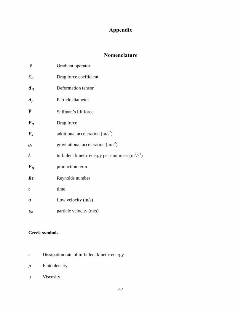
67

Appendix

Nomenclature

∇ Gradient operator

𝑪𝒅 Drag force coefficient

𝒅𝒊𝒋 Deformation tensor

𝒅𝒑 Particle diameter

�⃗⃗⃗⃗� Saffman’s lift force

𝑭𝑫 Drag force

Fx additional acceleration (m/s2)

gx gravitational acceleration (m/s2)

k turbulent kinetic energy per unit mass (m2/s

2)

𝑷𝒊𝒋 production term

Re Reynolds number

t time

u flow velocity (m/s)

up particle velocity (m/s)

Greek symbols

휀 Dissipation rate of turbulent kinetic energy

𝜌 Fluid density

μ Viscosity

68

𝜌p particle density

Subscripts

i, j, k unit vectors in x, y and z directions

p particle

d drag

Abbreviations

BC boundary condition

CFD computational fluid dynamics

DPM discrete phase model

DRW discrete random walk

FVM finite volume method

RSTM Reynolds stress turbulence modelling

SIMPLEC Semi-Implicit Method for Pressure-Linked Equations-Consistent

69

Curriculum Vita

Antara Badhan, only one child of Md. Abdur Rahman Mia and Nurzahan Begum, was

born on 21st September, 1989 in Dhaka, Bangladesh. Ms. Badhan completed her secondary

school certificate from Monipur High School and higher secondary school certificate from

Dhaka City College, Bangladesh and then joined Khulna University of Engineering &

Technology (KUET) for Bachelor of Science in Civil Engineering in February, 2007. She has

completed her Bachelor degree in May 2011 from KUET. She gained knowledge on Engineering

Measurements (Land Surveying), Foundation engineering and Hydraulic Engineering during her

undergraduate course. Ms. Badhan joined the University of Texas at El Paso (UTEP) to pursue

Master of Science degree in Mechanical Engineering in January 2013. She has been working as a

Graduate Research Assistant in Computational Fluid Mechanics Lab. Her work was focused on

numerical analysis of particle flow inside a bio-aerosol cyclone sampler to evaluate particle

collection efficiency for different design options. . In addition to her research work, Ms. Badhan

served teaching assistant duties in last two semesters in undergraduate level Thermal System

Design. She has instructed ungraduated students on their experiments/labs session in Lockheed

Martin Mechanical Engineering Lab at UTEP. She is a coauthor of 2 conference papers to be

published this year and is currently working on a journal draft as well as other proposals.

Permanent Address: 73/a, Kadamtala, Bashaboo, Sabujbagh

Dhaka, Bangladesh.

Author’s Name: Antara Badhan