numerical modeling of rock deformation, stefan schmalholz, eth zurich numerical modeling of rock...
Post on 21-Dec-2015
235 views
TRANSCRIPT
Numerical modeling of rock deformation, Stefan Schmalholz, ETH Zurich
Numerical modeling of rock deformation:
14 FEM 2D Viscous folding
Stefan [email protected]
NO E 61
AS 2008, Thursday 10-12, NO D 11
Numerical modeling of rock deformation, Stefan Schmalholz, ETH Zurich
Folding: Mechanism
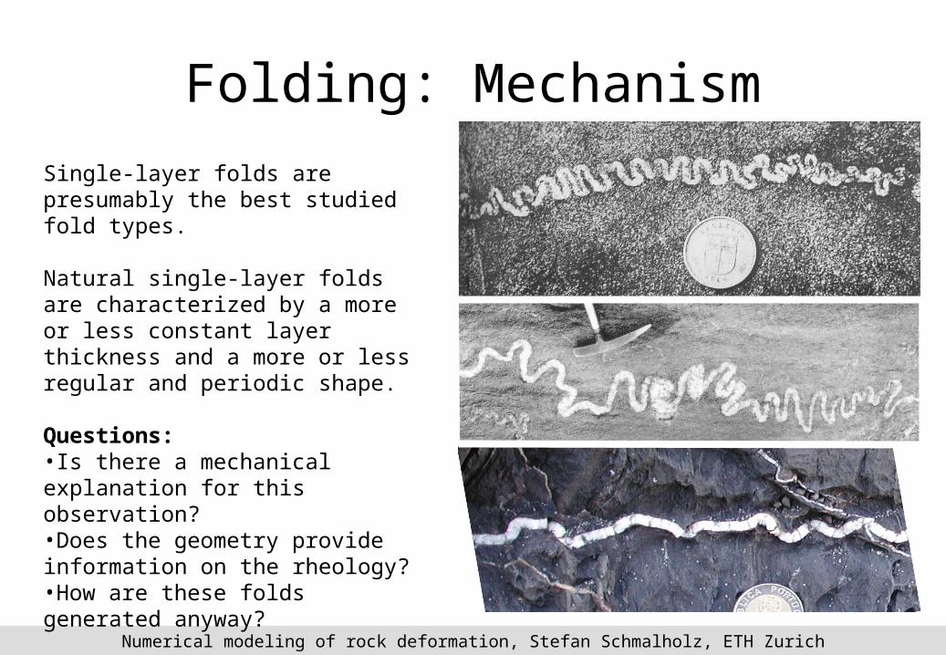
Single-layer folds are presumably the best studied fold types.
Natural single-layer folds are characterized by a more or less constant layer thickness and a more or less regular and periodic shape.
Questions:•Is there a mechanical explanation for this observation?•Does the geometry provide information on the rheology?•How are these folds generated anyway?
Numerical modeling of rock deformation, Stefan Schmalholz, ETH Zurich
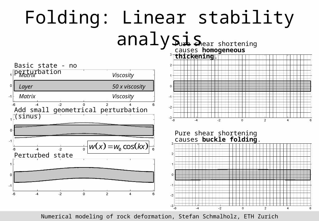
Folding: Linear stability analysisPure shear shortening causes homogeneous thickening.
Pure shear shortening causes buckle folding.
Basic state - no perturbation
Add small geometrical perturbation (sinus)
Perturbed state
Layer
Matrix
Matrix
50 x viscosity
Viscosity
Viscosity
0 cosw x w kx

Numerical modeling of rock deformation, Stefan Schmalholz, ETH Zurich
Folding: Linear stability analysis
0, exp cos 2 /w x t w t x
Is a layer with small sinusoidal perturbations stable under compression?Do small perturbations grow very fast?
Homogeneous pure shear thickening of the layer is:
stable if < 0 shortening/thickeningneutrally stable if = 0 shortening/thickeningand unstable if > 0 folding/buckling
Thin-plate equation for viscous folding.
12
H
w
2
Assuming exponential growth with time.
Partial differential equation. x
3 5 21
1 24 2
24 4 0
3
H w w wH
tx t x

Numerical modeling of rock deformation, Stefan Schmalholz, ETH Zurich
2
k
13 3
1 2
12
12
Hk
H k
The analytical solution for the growth rate of the wavelength components is
0, exp cos 2 /w x t w t x
1
0
ln /w
dtw
The analytical form for the amplitude, w, evolution considering the background shortening rate is
The numerical form for the amplitude evolution is
1 0 expw w dt
The growth rate can be calculated from the numerically calculated amplitude
1
0
amplitude after one time step
initial amplitude
time step
shortening rate
w
w
dt

Numerical modeling of rock deformation, Stefan Schmalholz, ETH Zurich
1 2
3 31 1
1 12 2
4 2 ,
6 3H
Plot the analytical growth rate and the numerical growth rate for different values of the wavelength (model width). Tips:-make a loop that changes the model width (i.e. wavelength) automatically-Only make one time step-Use a small time step and a small initial amplitude-You can extract the layer interface from the YCOORD array with the vector Ind_lay.
Test the formulas for the maximal value of the growth rate and for the dominant wavelength, i.e. the wavelength for which the growth rate is maximal.
Such tests are very important to test numerical algorithms and evaluate their accuracy.
The analytical solution is an approximate, thin-plate solution, because it neglects the shear deformation and shear strains during folding. Describe the difference between the analytical and numerical solution and explain them.You can also add a random perturbation on the layer interface and test whether the resulting fold shapes are close to the ones predicted by the analytical solution, such as on the next page.

Numerical modeling of rock deformation, Stefan Schmalholz, ETH Zurich
1
1
Dispersion curve
1
31
12
26
H
~1 ~1
2
31
12
46
Biot, 1957Ramberg, 1963
Numerical verification

Numerical modeling of rock deformation, Stefan Schmalholz, ETH Zurich
This is what you should get
Viscosity ratio = 100