numerical methods - unibspaola-gervasio.unibs.it/nummeth/intro_s.pdf · numerical analysis is a...
TRANSCRIPT
Numerical Methods
PhD Program in Natural Risks Assessment and Management(NRAM)
Spring 2012
Paola Gervasio
e-mail: [email protected] web: http://dm.ing.unibs.it/gervasiotel.: 030 371 5734
c©Paola Gervasio - Numerical Methods - 2012 1

What is Numerical Analysis
Numerical Analysis is a part of mathematics that investigates andstudies efficient methods for computing approximated solutions ofphysical problems modeled by mathematical systems.
Mathematical language
Computers
Approximation Techniques
Efficiency
c©Paola Gervasio - Numerical Methods - 2012 2
Some physical problems:
Fluid dynamicsGoal: Weather forecast, tsunami preventionGoal: monitoring and reporting the spread of ashesGoal: simulation of the fluid dynamics around obstacles
Offshore Platform DesignGoal: to develop a sound, reliable, and safe operating platform
Ice Sheet modelingGoal: to model the three-dimensional motion of a glacier
c©Paola Gervasio - Numerical Methods - 2012 3

...
Google searchGoal: quick and careful surfing on the web
Image compression and refinementComputer graphics, rendering, textiles simulation,...
c©Paola Gervasio - Numerical Methods - 2012 4
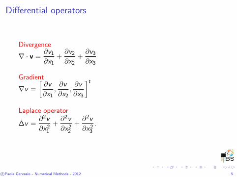
Differential operators
Divergence
∇ · v =∂v1
∂x1+
∂v2
∂x2+
∂v3
∂x3
Gradient
∇v =
[
∂v
∂x1,
∂v
∂x2,
∂v
∂x3
]t
Laplace operator
∆v =∂2v
∂x21
+∂2v
∂x22
+∂2v
∂x23
.
c©Paola Gervasio - Numerical Methods - 2012 5
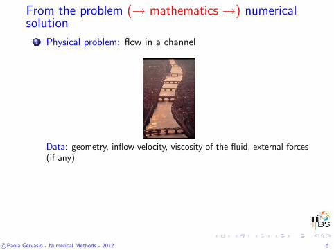
From the problem (→ mathematics →) numericalsolution
1 Physical problem: flow in a channel
Data: geometry, inflow velocity, viscosity of the fluid, external forces(if any)
c©Paola Gervasio - Numerical Methods - 2012 6

From the problem (→ mathematics →) numericalsolution
1 Physical problem: flow in a channel
2 Mathematical model: Incompressible Navier-Stokes equationswe want to look for velocity v = v(t, x) and pressurep = p(t, x), which are the solutions of
∂v
∂t− ν∆v + v · (∇v) + ∇p = f in Ω × (0,T )
∇ · v = 0 in Ω × (0,T )b.c. + i.c.
c©Paola Gervasio - Numerical Methods - 2012 7

From the problem (→ mathematics →) numericalsolution
1 Physical problem: flow in a channel
2 Mathematical model: Incompressible Navier-Stokes equations
3 Numerical approximation and algorithmsapproximation of derivatives, integrals, ...a small piece of a matlab program:for t = tspan(1)+dt:dt:tspan(2)
fn1 = f(xh,t);
rhs = An*[un;vn]+[dt*dt*zeta*fn1+dt*dt*(0.5-zeta)*fn;
dt*theta1*fn1+theta*dt*fn1];
rhs(1) = g(xspan(1),t); rhs(N)=g(xspan(2),t);
rhs(N+1:end)=rhs(N+1:end)-An211*temp1-An212*temp2;
uh = L\rhs; uh = U\uh;fn = fn1; un = uh(1:N); vn = uh(N+1:end); uhg=[uhg,un];
end
c©Paola Gervasio - Numerical Methods - 2012 8
From the problem (→ mathematics →) numericalsolution
1 Physical problem: flow in a channel
2 Mathematical model: Incompressible Navier-Stokes equations
3 Numerical approximation and algorithmsThe discrete solution is (vh, ph), it depends on thediscretization size h and in general it does not coincide withthe exact solution (v, p).
c©Paola Gervasio - Numerical Methods - 2012 9
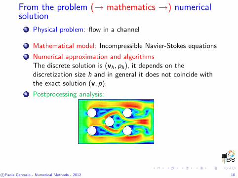
From the problem (→ mathematics →) numericalsolution
1 Physical problem: flow in a channel
2 Mathematical model: Incompressible Navier-Stokes equations
3 Numerical approximation and algorithmsThe discrete solution is (vh, ph), it depends on thediscretization size h and in general it does not coincide withthe exact solution (v, p).
4 Postprocessing analysis:
c©Paola Gervasio - Numerical Methods - 2012 10
The continuous problem
Mathematical Analysis
Is the problem well posed?
That is: there exists a unique solution and does it continuouslydepend on data? (= Do small changes on data provide smallchanges on the solution?)
c©Paola Gervasio - Numerical Methods - 2012 11
How can we find the solution?
Mathematical analysis often does not provide explicit rules to findthe solution, or sometimes the rules exist but are very complex tobe implemented
We have to look for approximated solutions by computers
But digital computers are not able to compute exact derivatives,integrals and all of what refers to the “limit” lim
t→0f (t)
Attention: We are not interested in computing derivatives andintegrals by symbolic tools (e.g.. Derive, Maple, Mathematica, ....)since they do not go beyond the rules of mathematical analysis.
c©Paola Gervasio - Numerical Methods - 2012 12

From mathematical analysis to numerical analysis
We have to translate the continuous problem in a discrete one:
1 Domain discretization: choose some points in the domain (afew: ≃ 102, lots of: ≃ 106, but the number is always finite) atwhich to look for the approximated (or numerical) solution.h is the discretization ”size”
h
c©Paola Gervasio - Numerical Methods - 2012 13
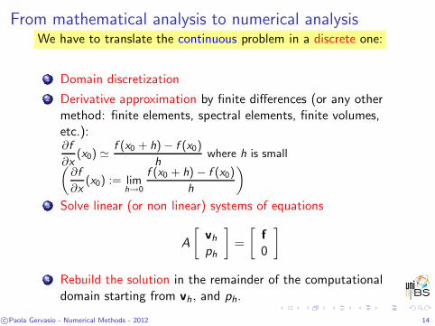
From mathematical analysis to numerical analysisWe have to translate the continuous problem in a discrete one:
1 Domain discretization
2 Derivative approximation by finite differences (or any othermethod: finite elements, spectral elements, finite volumes,etc.):∂f
∂x(x0) ≃
f (x0 + h) − f (x0)
hwhere h is small
(
∂f
∂x(x0) := lim
h→0
f (x0 + h) − f (x0)
h
)
3 Solve linear (or non linear) systems of equations
A
[
vh
ph
]
=
[
f
0
]
4 Rebuild the solution in the remainder of the computationaldomain starting from vh, and ph.
c©Paola Gervasio - Numerical Methods - 2012 14

Which are the goals of Numerical Analysis?
1 To propose discretization methods for mathematical problems.
2 To investigate if, when h → 0, the numerical solution (vh, ph)converges to the exact one (v, p) (theoretical study)
3 To translate numerical methods in efficient (in terms ofCPU-time and memory allocation) and stable (less sensible aspossible to machine arithmetic) algorithms
4 To verify the results
Ween need both mathematical and computational knowledges
c©Paola Gervasio - Numerical Methods - 2012 15
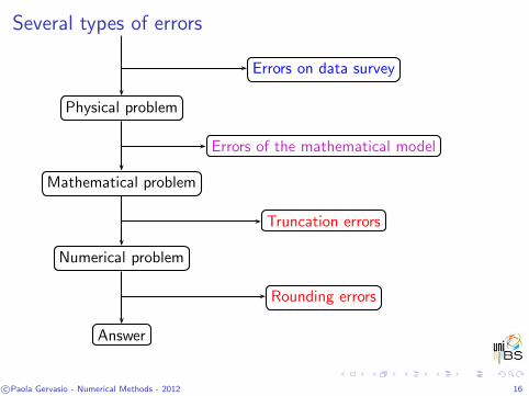
Several types of errors
Errors on data survey
Physical problem
Errors of the mathematical model
Mathematical problem
Truncation errors
Numerical problem
Rounding errors
Answer
c©Paola Gervasio - Numerical Methods - 2012 16

Truncation (or approximation) errors
In approximating f ′(x0) ≃f (x0 + h) − f (x0)
hwe introduce an error.
Write the Taylor 1st-order expansion of f (x) centered in x0:
f (x) = f (x0) + f ′(x0)(x − x0) + f′′(ξ)2 (x − x0)
2.
Set x = x0 + h:
f (x0 + h) = f (x0) + f ′(x0)(x0 + h − x0) +f ′′(ξ)
2(x0 + h − x0)
2,
explicit f ′(x0) and it holds:
f ′(x0) =f (x0 + h) − f (x0)
h−
f ′′(ξ)
2h
The error introduced in this approximation is of truncation typesince we have cut off the Taylor expansion of f to approximate f ′.
c©Paola Gervasio - Numerical Methods - 2012 17
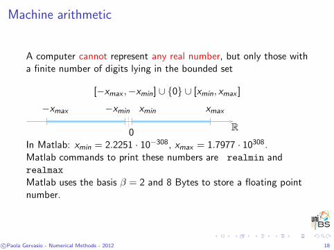
Machine arithmetic
A computer cannot represent any real number, but only those witha finite number of digits lying in the bounded set
[−xmax ,−xmin] ∪ 0 ∪ [xmin, xmax ]
−xmin−xmax xmin xmax
0R
In Matlab: xmin = 2.2251 · 10−308, xmax = 1.7977 · 10308.Matlab commands to print these numbers are realmin andrealmax
Matlab uses the basis β = 2 and 8 Bytes to store a floating pointnumber.
c©Paola Gervasio - Numerical Methods - 2012 18

Rounding errors
To represent a number, the computer introduces an error(rounding error) characterized by the basis β and the number t ofbits used to store the mantissa of the number itself:
|x − flt(x)| ≤1
2β1−t |x |
Matlab uses β = 2 and t = 53,12β1−t = 1.1102 · 10−16
c©Paola Gervasio - Numerical Methods - 2012 19
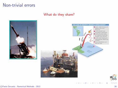
Non-trivial errors
What do they share?
c©Paola Gervasio - Numerical Methods - 2012 20

February, 25 1991: A Patriot missile fails in hitting a SCUDmissile, the latter falls on U.S. barrack: 28 people died.Why?The excessive propagation of rounding errors (in measuring time)gives rise to a large error in computing the trajectory of the missile.
c©Paola Gervasio - Numerical Methods - 2012 21
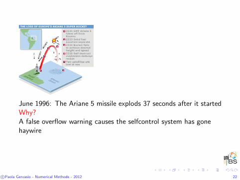
June 1996: The Ariane 5 missile explods 37 seconds after it startedWhy?A false overflow warning causes the selfcontrol system has gonehaywire
c©Paola Gervasio - Numerical Methods - 2012 22
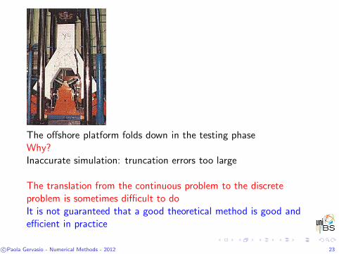
The offshore platform folds down in the testing phaseWhy?Inaccurate simulation: truncation errors too large
The translation from the continuous problem to the discreteproblem is sometimes difficult to doIt is not guaranteed that a good theoretical method is good andefficient in practice
c©Paola Gervasio - Numerical Methods - 2012 23
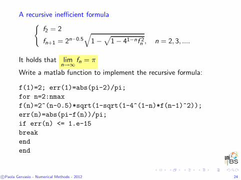
A recursive inefficient formula
f2 = 2
fn+1 = 2n−0.5√
1 −√
1 − 41−nf 2n , n = 2, 3, ....
It holds that limn→∞
fn = π
Write a matlab function to implement the recursive formula:
f(1)=2; err(1)=abs(pi-2)/pi;
for n=2:nmax
f(n)=2^(n-0.5)*sqrt(1-sqrt(1-4^(1-n)*f(n-1)^2));
err(n)=abs(pi-f(n))/pi;
if err(n) <= 1.e-15
break
end
end
c©Paola Gervasio - Numerical Methods - 2012 24
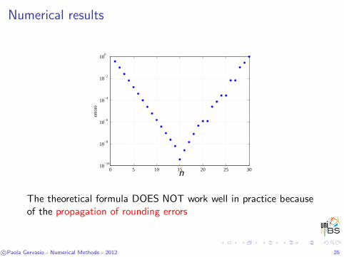
Numerical results
0 5 10 15 20 25 3010
−10
10−8
10−6
10−4
10−2
100
erro
re
n
The theoretical formula DOES NOT work well in practice becauseof the propagation of rounding errors
c©Paola Gervasio - Numerical Methods - 2012 25
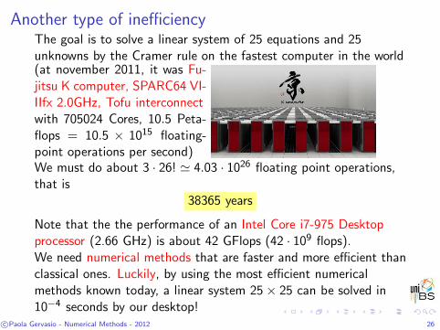
Another type of inefficiencyThe goal is to solve a linear system of 25 equations and 25unknowns by the Cramer rule on the fastest computer in the world(at november 2011, it was Fu-jitsu K computer, SPARC64 VI-IIfx 2.0GHz, Tofu interconnectwith 705024 Cores, 10.5 Peta-flops = 10.5 × 10¹⁵ floating-point operations per second)We must do about 3 · 26! ≃ 4.03 · 1026 floating point operations,that is
38365 years
Note that the the performance of an Intel Core i7-975 Desktopprocessor (2.66 GHz) is about 42 GFlops (42 · 109 flops).We need numerical methods that are faster and more efficient thanclassical ones. Luckily, by using the most efficient numericalmethods known today, a linear system 25 × 25 can be solved in10−4 seconds by our desktop!
c©Paola Gervasio - Numerical Methods - 2012 26
References
A. Quarteroni, F. Saleri.Calcolo Scientifico,
4a ed. Springer Italia, Milano, 2008.
A. Quarteroni, F. Saleri, P. Gervasio.Scientific Computing with Matlab and
Octave,
3rd ed. Springer, Berlin, 2010.
c©Paola Gervasio - Numerical Methods - 2012 27