numerical methods slides - jcthomedir.jct.ac.il/~naiman/nm/nm-slides-color.pdftaylor...

Numerical Methods

Aaron NaimanJerusalem College of Technology

[email protected]

http://jct.ac.il/∼naiman

based on: Numerical Mathematics and Computing

by Cheney & Kincaid, c©1994

Brooks/Cole Publishing Company

ISBN 0-534-20112-1

Copyright c©2014 by A. E. Naiman

Taylor Series

⇒ Definitions and Theorems

• Examples

• Proximity of x to c

• Additional Notes

Copyright c©2014 by A. E. Naiman NM Slides —Taylor Series, p. 1

http://jct.ac.il/~naiman/nm

Motivation

• Sought: cos (0.1)

• Missing: calculator or lookup table

• Known: cos for another (nearby) value, i.e., at 0

• Also known: lots of (all) derivatives at 0

• Can we use them to approximate cos (0.1)?

• What will be the worst error of our approximation?

These techniques are used by computers, calculators, tables.



Taylor Series — cosx

-1.5

-1

-0.5

0

0.5

1

1.5

-4 -2 0 2 4

function

value

cosx

1

1− x2

2

1− x2

2 + x4

4!

1− x2

2 + x4

4!− x6

6!

I

z

z

Other series

Better and better approximation, near c, and away.


http://demonstrations.wolfram.com/GraphsOfTaylorPolynomials


Taylor Series

• Series definition: If ∃f(k)(c), k = 0,1,2, . . ., then:

f(x) ≈ f(c) + f ′(c)(x− c) +f ′′(c)2!

(x− c)2 + · · ·

=∞∑

k=0

f(k)(c)

k!(x− c)k

• c is a constant and much is known about it (f(k)(c))

• x a variable near c, and f(x) is sought

• With c = 0 ⇒ Maclaurin series

• What is the maximum error if we stop after n terms?

• Real life: crowd estimation: 100K ±10K vs. 100K ±1K

Key NM questions: What is estimate? What is its max error?



Taylor’s Theorem

• Theorem: If f ∈ Cn+1[a, b] then

f(x) =n∑

k=0

f(k)(c)

k!(x− c)k +

f(n+1)(ξ(x))

(n+1)!(x− c)n+1

where

x, c ∈ [a, b], ξ(x) ∈ open interval between x and c

• Notes:

∗ f ∈ C(X) means f is continuous on X

∗ f ∈ Ck(X) means f, f ′, f ′′, f(3), . . . , f(k) are continuous

on X

∗ ξ = ξ(x), i.e., a point whose position is a function of x

∗ Error term is just like other terms, with k := n+1

ξ-term is “truncation error”, due to series termination



Taylor Series—Procedure

• Setup: writing it out, step-by-step:

∗ write formula for f(k)(x)

∗ choose c (if not already specified)

∗ write out summation and error term

⋆ note: sometimes easier to write out a few terms

• Things to (possibly) prove — by analyzing worst case ξ

∗ analytically: letting n→∞⋆ LHS remains f(x)

⋆ summation becomes infinite Taylor series

⋆ if error term → 0 ⇒infinite Taylor series represents f(x)

∗ numerically: for given n, what is max of error term?



Taylor Series

• Definitions and Theorems

⇒ Examples





Taylor Series: ex

• f(x) = ex, |x| <∞ · ·· f(k)(x) = ex,∀k

• Choose c := 0

• We have

ex =n∑

k=0

xk

k!+

eξ(x)

(n+1)!xn+1

• As n→∞ — take worst case ξ (x > 0: just less than x;

x < 0?)

error term → 0 (why?) · ··

ex =∞∑

k=0

xk

k!= 1+ x+

x2

2!+

x3

3!+ · · ·



Taylor Series: sinx

• f(x) = sin x, |x| <∞ · ·· f(k)(x) = sin(

x+ πk2

)

,∀k, c := 0

• We have

sinx =n∑

k=0

sin(πk2

)

k!xk +

sin(

ξ(x) +π(n+1)

2

)

(n+1)!xn+1

• Error term → 0 as n→∞

• Even k terms are zero · ·· ℓ = 0,1,2, . . ., and k→ 2ℓ+1

sin x =∞∑

ℓ=0

sin(π(2ℓ+1)

2

)

(2ℓ+1)!x2ℓ+1 =

∞∑

k=0

(−1)kx2k+1

(2k+1)!= x−x3

3!+

x5

5!−· · ·



Taylor Series: cosx

• f(x) = cos x, |x| <∞ · ·· f(k)(x) = cos(

x+ πk2

)

,∀k, c := 0

• We have

cosx =n∑

k=0

cos(πk2

)

k!xk +

cos(

ξ(x) +π(n+1)

2

)

(n+1)!xn+1

• Error term → 0 as n→∞

• Odd k terms are zero · ·· ℓ = 0,1,2, . . ., and k → 2ℓ

cos x =∞∑

ℓ=0

cos(π(2ℓ)

2

)

(2ℓ)!x2ℓ =

∞∑

k=0

(−1)k x2k

(2k)!= 1− x2

2!+

x4

4!− · · ·



Numerical Example: cos (0.1)

• We have 1)f(x) = cos x and 2)c = 0

∗ obtain series: cosx = 1− x2

2! +x4

4! − · · ·• Actual value: cos (0.1) = 0.99500416527803 . . .

• With 3)x = 0.1 and 4)specific n’s

∗ from Taylor approximations:

n∗ approximation |error| ≤0, 1 1 0.01/2!2, 3 0.995 0.0001/4!4, 5 0.99500416 0.000001/6!6, 7 0.99500416527778 0.00000001/8!... ... ...∗includes odd k

• Can also ask: given tolerance τ , what n is needed?

Obtain accurate approximation easily and quickly.



Taylor Series: (1− x)−1

• f(x) = 11−x, 6 ∃f(1)⇒ 1 6∈ [a, b]; below: error 6→ 0 for x ≤ −1

• · ·· |x| < 1, f(k)(x) = k!

(1−x)k+1,∀k, choose c := 0

• We have

1

1− x=

n∑

k=0

xk +(n+1)!

(1− ξ(x))n+2· xn+1

(n+1)!

=n∑

k=0

xk +

(

x

1− ξ(x)

)n+11

1− ξ(x)

• Why bother, with LHS so simple? Ideas?

• Problem: actually ξ = ξ(n); 1− ξ(x)→∞? Solution . . .

• Later: x bdd away from 1 · ·· suff.:∣∣∣

x1−ξ(x)

∣∣∣n+1 → 0 as n→∞

• For what range of x is this satisfied?

Need to determine radius of convergence.



(1− x)−1 — Range of Convergence

• Sufficient:∣∣∣

x1−ξ(x)

∣∣∣ < 1

• Approach:

∗ get variable x in middle of sufficiency inequality

∗ transform range of ξ inequality to LHS and RHS of

sufficiency inequality

∗ require restriction on x

⋆ but check if already satisfied

• |ξ| < 1 ⇒ 1− ξ > 0 ⇒ sufficient: −(1− ξ) < x < 1− ξ



(1− x)−1 — Range of Convergence (cont.)

• case x < ξ < 0:

∗ LHS: −(1− x) < −(1− ξ) < −1 ⇒ require: −1 ≤ x√

∗ RHS: 1 < 1− ξ < 1− x ⇒ require: x ≤ 1√

• case 0 < ξ < x:

∗ LHS: −1 < −(1− ξ) < −(1− x) ⇒ require: −(1− x) ≤ x,

or: −1 < 0√

∗ RHS: 1− x < 1− ξ < 1 ⇒ require: x ≤ 1− x, or: x ≤ 12

• Therefore, for −1 < x ≤ 12

1

1− x=∞∑

k=0

xk = 1+ x+ x2 + x3 + · · ·(

Zeno: x = 12, . . .

)

Need more analysis for the whole range |x| < 1.



Taylor Series: lnx

• f(x) = ln x, 0 < x ≤ 2 · ·· f(k)(x) = (−1)k−1(k−1)!xk

,∀k ≥ 1

• Choose c := 1

• We have

lnx =n∑

k=1

(−1)k−1(x− 1)k

k+ (−1)n 1

n+1

(x− 1)n+1

ξn+1(x)

• Sufficient∣∣∣x−1ξ(x)

∣∣∣n+1 → 0 as n→∞

• Again, for what range of x is this satisfied?



lnx — Range of Convergence• Sufficient:

∣∣∣x−1ξ(x)

∣∣∣ < 1 . . . 1− ξ < x < 1+ ξ

• case 1 < ξ < x:

∗ LHS: 1− x < 1− ξ < 0 ⇒ require: 0 ≤ x√

∗ RHS: 2 < 1+ ξ < 1 + x ⇒ require: x ≤ 2√

• case x < ξ < 1:

∗ LHS: 0 < 1− ξ < 1− x ⇒ require: 1− x ≤ x, or: 12 ≤ x

∗ RHS: 1 + x < 1 + ξ < 2 ⇒ require: x ≤ 1+ x√

• Therefore, for 12 ≤ x ≤ 2

ln x =∞∑

k=1

(−1)k−1(x− 1)k

k= (x− 1)− (x− 1)2

2+

(x− 1)3

3− · · ·

Again, need more analysis for entire range of x.



Ratio Test and lnx Revisited

• Theorem:∣∣∣an+1an

∣∣∣→ (< 1) ⇒ partial sums converge

• ln x: ratio of adjacent summand terms (not the error term)∣∣∣∣

an+1

an

∣∣∣∣ =

∣∣∣∣(x− 1)

n

n+1

∣∣∣∣

• Obtain convergence of partial sums for 0 < x < 2

• Note: not looking at ξ and the error term

• x = 2: 1− 12 + 1

3 − · · ·, which is convergent (why?)

• x = 0: same series, all same sign ⇒ divergent harmonic series

• · ·· we have 0 < x ≤ 2



(1− x)−1 Revisited

• Letting x→ (1− x)

ln (1− x) = −(

x+x2

2+

x3

3+ · · ·

)

, −1 ≤ x < 1

• ddx: lhs = −1

1−x and rhs = −(

1+ x+ x2 + x3 + · · ·)

• ! : no “=” for x = −1 as rhs oscillates (note: correct avg

value)

• |x| < 1 we have (also with ratio test)

1

1− x= 1+ x+ x2 + x3 + · · ·



Taylor Series


• Examples

⇒ Proximity of x to c




Proximity of x to c

Problem: Approximate ln 2

• Solution 1: Taylor ln (1 + x) around 0 with x = 1

ln2 = 1− 1

2+

1

3− 1

4+

1

5− 1

6+

1

7− 1

8+ · · ·

• Solution 2: Taylor ln(1+x1−x

)

around 0 with x = 13

ln 2 = 2

(

3−1 +3−3

3+

3−5

5+

3−7

7+ · · ·

)



Proximity of x to c (cont.)

• Approximated values, rounded:

∗ Solution 1, first 8 terms: 0.63452

∗ Solution 2, first 4 terms: 0.69313

• Actual value, rounded: 0.69315

• · ·· importance of proximity of evaluation and expansion points

• Accuracy and proximity and for varying c

This error is in addition to the truncation error.


http://demonstrations.wolfram.com/AccuracyOfSeriesApproximations

http://demonstrations.wolfram.com/TaylorPolynomials


Taylor Series


• Examples


⇒ Additional Notes



Polynomials and a Second Form• Polynomials ∈ C∞(−∞,∞)

∗ have finite number of non-zero derivatives, · ··∗ Taylor series ∀c . . . original polynomial, i.e., error = 0

f(x) = 3x2−1, . . . f(x) =2∑

k=0

f(k)(0)

k!xk = −1+0+3x2

∗ Taylor Theorem can be used for fewer terms

⋆ e.g.: approximate a P17 near c by a P3

• Taylor’s Theorem, second form (x = constant expansion

point, h = distance, x+ h = variable evaluation point):

If f ∈ Cn+1[a, b] then

f(x+ h) =n∑

k=0

f(k)(x)

k!hk +

f(n+1)(ξ(h))

(n+1)!hn+1

x, x+ h ∈ [a, b], ξ(h) ∈ open interval between x and x+ h



Taylor Approximate: (1− 3h)45

• Define: f(z) ≡ z45; x = 1 is the constant expansion point

• Derivs: f ′(z) = 45z−1

5, f ′′(z) = − 452

z−65, f ′′′(z) = 24

53z−

115 , . . .

• · ·· :

(x+ h)45 = x

45 +

4

5x−

15h− 4

2! · 52x−6

5h2 +24

3! · 53x−11

5 h3 + . . .

(x− 3h)45 = x

45− 4

5x−

153h− 4

2! · 52x−

659h2− 24

3! · 53x−

115 27h3+ . . .

(1− 3h)45 = 1− 4

53h− 4

2! · 529h2 − 24

3! · 5327h3 + . . .

= 1− 12

5h− 18

25h2 − 108

125h3 + . . .



Second Form — ln (e+ h)

• Evaluation of interest: ln (e+ h), for −e < h ≤ e

• Define: f(z) ≡ ln (z)

• x = e is the constant expansion point

• ln ⇒ z > 0

• Derivatives

f(z) = ln z f(e) = 1

f ′(z) = z−1 f ′(e) = e−1

f ′′(z) = −z−2 f ′′(e) = −e−2f ′′′(z) = 2z−3 f ′′′(e) = 2e−3

f(n)(z) = (−1)n−1(n− 1)!z−n f(n)(e) = (−1)n−1(n− 1)! e−n



ln (e+ h) — Expansion and Convergence• Expansion (recall: x = e)

ln (e+ h) ≡ f(x+ h) = 1+n∑

k=1

(−1)k−1(k − 1)!e−khk

k!+

(−1)n n! ξ(h)−(n+1)hn+1

(n+1)!

or

ln (e+ h) = 1+n∑

k=1

(−1)k−1k

(h

e

)k

+(−1)nn+1

(

h

ξ(h)

)n+1

• Range of convergence, sufficient (for variable h): −ξ < h < ξ

∗ case e+ h < ξ < e: . . . −e2 ≤ h

∗ case e < ξ < e+ h: . . . h ≤ e

• Can prove with: ln (e+ h) = ln(

e(

1+ he

))

= 1+ ln(

1+ he

)

,

and prev. section



O() Notation and MVT• As h→ 0, we write the speed of f(h)→ 0

f(h) = O(

hk)

≡ |f(h)| ≤ C|h|k

e.g., f(h): h, 11000h, h2; let h→ 1

10,1

100,1

1000, . . .

• Taylor truncation error = O(

hn+1)

; if for a given n the max

exists, then

C :=

∣∣∣∣∣maxξ(h)

f(n+1)(ξ(h))

∣∣∣∣∣/(n+1)!

• Mean value theorem (Taylor, n = 0): If f ∈ C1[a, b] then

f(b) = f(a) + (b− a)f ′(ξ), ξ ∈ (a, b)

or:

f ′(ξ) =f(b)− f(a)

b− a



Alternating Series Theorem

• Alternating series theorem: If ak > 0, ak ≥ ak+1, ∀k ≥ 0, and

ak → 0, then

n∑

k=0

(−1)kak → S and |S − Sn| ≤ an+1

• Intuitively understood

• Note: direction of error is also know for specific n

• We had this with sin and cos

• Another useful method for max truncation error estimation

Max truncation error estimation without ξ-analysis



ln (e+ h) — Max Trunc. Error Estimate• What is the max error after n+1 terms?

• Max error estimate also depends on proximity—size of h∗ from Taylor: obtain O

(

hn+1)

|error| ≤ 1

n+1|h|n+1max

ξ

∣∣∣∣∣

1

ξ

∣∣∣∣∣

n+1

∗ from AST (check the conditions!): also obtain

O(

hn+1)

, with different constant

|error| ≤ 1

n+1

∣∣∣∣

h

e

∣∣∣∣

n+1

• E.g.: h = e2: ln e

2 = 1+ 12 −

12 ·

122

+ 13 ·

123− 1

4 ·124

+ · · ·∗ Taylor max error (occurs as ξ → e+): 1

n+1 ·1

2n+1

∗ AST max error: 1n+1 ·

12n+1

∗ note same ln estimate (before); in this case only, samemax error estimate as well (not in general)



Base Representations

⇒ Definitions

• Conversions

• Computer Representation

• Loss of Significant Digits

Copyright c©2014 by A. E. Naiman NM Slides —Base Representations, p. 1


Number Representation

• Simple representation in one base 6⇒ simple representation in

another base, e.g.

(0.1)10 = (0.0 0011 0011 0011 . . .)2

• Base 10:

37294 = 4+ 90+ 200+ 7000 + 30000

= 4× 100 +9× 101 +2× 102 +7× 103 +3× 104

in general: an . . . a0 =n∑

k=0

ak10k



Fractions and Irrationals

• Base 10 fraction:

0.7217 = 7× 10−1 +2× 10−2 +1× 10−3 +7× 10−4

• In general, for real numbers:

an . . . a0.b1 . . . =n∑

k=0

ak10k +

∞∑

k=1

bk10−k

• Note: ∃ numbers, i.e., irrationals, such that an infinite number

of digits are required, in any rational base, e.g., e, π,√2

• Need infinite number of digits in a base 6⇒ irrational

(0.333 . . .)10 but1

3is not irrational

but, if rational, digits will repeat, e.g.: 0.312461



Other Bases

• Base 8, 6 ∃ ‘8’ or ‘9’, using octal digits

(21467)8 = · · · = (9015)10

(0.36207)8 = 8−5(

3× 84 + · · ·)

=15495

32768= (0.47286 . . .)10

• Base 16: ‘0’, ‘1’, . . . , ‘9’, ‘A’ (10), ‘B’ (11), ‘C’ (12), ‘D’

(13), ‘E’ (14), ‘F’ (15)

• Base β

(an . . . a0.b1 . . .)β =n∑

k=0

akβk +

∞∑

k=1

bkβ−k

• Base 2: just ‘0’ and ‘1’, or for computers: “off” and “on”,

“bit” = binary digit




• Definitions

⇒ Conversions





Conversion: Base 10 → Base 2• Basic idea:

3781 = 1+ 10︸︷︷︸(1010)2

8︸︷︷︸(1000)2

+10(7+ 10(3))

= · · ·

= (111 011 000 101)2

• Easy for computer, but by hand: (3781.372)10

remainder2)3781 ·2)1890 1 = a0 ↓2)945 0 = a1

...

0.372· 2

↓ b1 = 0 .7442

b2 = 1 .488 (drop 1 )...

• Valid from/to any base; one digit for each ∗/÷

• Usually from base 10, with familiar ∗/÷Copyright c©2014 by A. E. Naiman NM Slides —Base Representations, p. 6


Base 8 Shortcut

• Base 2 ↔ base 8, trivial

(551.624)8 = (101 101 001.110 010 100)2

• ≈ 3 bits for every 1 octal digit

• One digit produced for every step in (hand) conversion

• · ·· base 10 → base 8 → base 2

• For base 8 ↔ base 16: via base 2




• Definitions

• Conversions

⇒ Computer Representation




Computer Representation

• Scientific notation:

32.213→ 0.32213× 102

• In general

x = ±0.d1d2 . . .× 10n, d1 6= 0, or: x = ±r × 10n,1

10≤ r < 1

we have sign, “mantissa” r and “exponent” n

• On the computer, base 2 is represented

x = ±0.b1b2 . . .× 2n, b1 6= 0, or: x = ±r × 2n,1

2≤ r < 1

• Finite number of mantissa digits, therefore “roundoff” or

“truncation” error




• Definitions

• Conversions


⇒ Loss of Significant Digits



LSD—Addition

• (a+ b) + c = a+ (b+ c) on the computer?

• Six decimal digits for mantissa

1,000,000.+1.+ · · ·+1.︸︷︷︸

million times

= 1,000,000.

because

0.100000× 107 +0.100000× 101 = 0.100000× 107

but

1.+ · · ·+1.︸︷︷︸

million times

+1,000,000. = 2,000,000.

Add numbers in size order.



LSD—Subtraction

• Assume 10 decimal digits of precision ( N[] or vpa() )

• E.g.: x− sin x for x’s close to zero

x =1

15(radians)

x = 0.66666 66667× 10−1

sinx = 0.66617 29492× 10−1

x− sinx = 0.00049 37175× 10−1

= 0.49371 75000× 10−4

• Note

∗ still have 10−10 precision (because no more info), but

∗ can we rework calculation for 10−13 precision?

Avoid subtraction of close numbers.


http://reference.wolfram.com/mathematica/ref/N.html

http://www.mathworks.com/help/symbolic/vpa.html


LSD Avoidance for Subtraction

• x− sinx for x ≈ 0 → use Taylor series

∗ no subtraction of close numbers

∗ e.g., 3 terms: 0.49371 74328× 10−4

actual: 0.49371 74327× 10−4

• ex − e−2x for x ≈ 0 → use Taylor series twice and add

common powers

•√

x2 +1− 1 for x ≈ 0 → x2√x2+1+1

• cos2 x− sin2 x for x ≈ π4 → cos 2x

• ln x− 1 for x ≈ e → ln xe



Nonlinear Equations

⇒ Motivation

• Bisection Method

• Newton’s Method

• Secant Method

• Summary

Copyright c©2014 by A. E. Naiman NM Slides —Nonlinear Equations, p. 1


Motivation

• For a given function f(x), find its root(s), i.e.:

⇒ find x (or r = root) such that f(x) = 0

• BVP: dipping of suspended power cable. What is λ?

λ cosh50

λ− λ− 10 = 0

• (Some) simple equations ⇒ solve analytically

6x2 − 7x+2 = 0

(3x− 2)(2x− 1) = 0

x =2

3,

1

2

cos3x− cos 7x = 0

2 sin 5x sin 2x = 0

x =nπ

5,nπ

2, n ∈ ZZ



Motivation (cont.)

• In general, we cannot exploit the function, e.g.:

2x2 − 10x+1 = 0

and

cosh

(√

x2 +1− ex)

+ log |sin x| = 0

• Note: at times ∃ multiple roots

∗ e.g., previous parabola and cosine

∗ we want at least one

∗ we may only get one (for each search)

Need a general, function-independent algorithm.



Nonlinear Equations

• Motivation

⇒ Bisection Method


• Secant Method

• Summary



Bisection Method—Example

-5

-4

-3

-2

-1

0

1

2

3

4

a bx0x1x2 x3

function

value

Intuitive, like guessing a number ∈ [0,100].



Restrictions and Max Error Estimate

• Restrictions of the Bisection Method

∗ function slices x-axis at root

⋆ start with two points a and b ∋− f(a)f(b) < 0

⋆ graphing tool (e.g., Matlab) can help to find a

and b

∗ require C0[a, b] (why? note: not a big deal)

• Max error estimate

∗ after n steps, guess midpoint of current range

∗ error: ǫ ≤ b−a2n+1 (think of n = 0,1,2)

∗ note: error is in x; can also look at error in f(x) or

combination

⋆ enters entire world of stopping criteria

Question: Given tolerance (in x), what is n? . . .


http://demonstrations.wolfram.com/BisectionMethod


Convergence Rate

• Given tolerance τ (e.g., 10−6), how many steps are needed?

• Tolerance restriction (ǫ from before):(

ǫ ≤ b− a

2n+1

)

< τ

• · ·· 1) × 2, 2) log (any base)

log (b− a)− n log2 < log 2τ

or

n >log (b− a)− log 2τ

log 2

Rate is independent of function.



Convergence Rate (cont.)

• Base 2 (i.e., bits of accuracy)

n > log2 (b− a)− 1− log2 τ

i.e., number of steps is a constant plus one step per bit

• Linear convergence rate: ∃C ∈ [0,1)∣∣∣xn+1 − r

∣∣∣ ≤ C|xn − r|, n ≥ 0

i.e., monotonic decreasing error at every step, and∣∣∣xn+1 − r

∣∣∣ ≤ Cn+1|x0 − r|

• Bisection convergence

∗ not linear (examples?), but compared to init. max error:

⇒ similar form:∣∣∣xn+1 − r

∣∣∣ ≤ Cn+1(b− a), with C = 1

2

Okay, but restrictive and slow.



Nonlinear Equations

• Motivation


⇒ Newton’s Method

• Secant Method

• Summary



Newton’s Method—Example

-0.2

0

0.2

0.4

0.6

0.8

1

1.2

x0x1x2x3

function

value

Other functions


http://demonstrations.wolfram.com/LearningNewtonsMethod


Newton’s Method—Definition

• Approximate f(x) near x0 by tangent ℓ(x)

f(x) ≈ f(x0) + f ′(x0)(x− x0) ≡ ℓ(x)

Want ℓ(r) = 0 ⇒ r = x0 − f(x0)f ′(x0)

, · ·· x1 := r, likewise:

xn+1 = xn −f(xn)

f ′(xn)

• Alternatively (Taylor’s): have x0, for what h is

f

x0 + h︸︷︷︸≡x1

= 0

f(x0 + h) ≈ f(x0) + hf ′(x0) or h = − f(x0)f ′(x0)



Convergence Rate

• English: With enough continuity and proximity ⇒quadratic convergence!

• Theorem: With the following three conditions:

1)f(r) = 0, 2)f ′(r) 6= 0, 3)f ∈ C2(

B(

r, δ))

⇒∃δ ∋−∀x0 ∈ B(r, δ) and ∀n we have

∣∣∣xn+1 − r

∣∣∣ ≤ C(δ)|xn − r|2

∗ for a given δ, C is a constant (not necessarily < 1)

• Note: again, use graphing tool to seed x0

Newton’s method can be very fast.



Convergence Rate Example

f(x) = x3 − 2x2 + x− 3, x0 = 4

n xn f(xn)0 4 331 3 92 2.4375 2.0368652343753 2.21303271631511 0.2563633850614184 2.17555493872149 0.006463361488813065 2.17456010066645 4.47906804996122e − 066 2.17455941029331 2.15717547991101e − 12

• Stopping criteria

∗ theorem: uses x; above: uses f(x)—often all we have

∗ possibilities: absolute/relative, size/change, x or f(x)

(combos, . . . )

But proximity issue can bite, . . . .



Sample Newton Failure #1

-4

-3

-2

-1

0

1

2

3

4

5

xn

function

value

Runaway process




-4

-2

0

2

4

xn

function

value

Division by zero derivative—recall algorithm




-2

-1.5

-1

-0.5

0

0.5

1

1.5

2

xnxn+1

function

value

Loop-d-loop (can happen over m points)



Nonlinear Equations

• Motivation



⇒ Secant Method

• Summary



Secant Method—Definition• Motivation: avoid derivatives

• Taylor (or derivative): f ′(xn) ≈ f(xn)−f(xn−1)xn−xn−1

• · ·· xn+1 = xn − f(xn)xn − xn−1

f(xn)− f(

xn−1) ( Secant Method )

• Bisection requirements comparison:

∗ √ 2 previous points

∗ × f(a)f(b) < 0

• Additional advantage vs. Newton:

∗ only one function evaluation per iteration

• Superlinear convergence:∣∣∣xn+1 − r

∣∣∣ ≤ C|xn − r|1.618...

(recognize the exponent?)


http://demonstrations.wolfram.com/SecantRootFindingMethod


Nonlinear Equations

• Motivation



• Secant Method

⇒ Summary



Root Finding—Summary

• Performance and requirementsf ∈ C2 nbhd(r) init. pts. speedy

bisection × × 2√

1 ×Newton

√ √1 × 2

√

secant × √2 × 1

√\requirement that f(a)f(b) < 0function evaluations per iteration

• Often methods are combined (how?), with restarts for

divergence or cycles

• Recall: use graphing tool to seed x0 (and x1)



Interpolation and Approximation

⇒ Motivation

• Polynomial Interpolation

• Numerical Differentiation


Copyright c©2014 by A. E. Naiman NM Slides —Interpolation and Approximation, p. 1


Motivation

• Three sample problems

∗ (xi, yi)|i = 0, . . . , n, (xi distinct), want simple (e.g.,

polynomial) p(x) ∋−yi = p(xi), i = 0, . . . , n ≡“interpolation”

∗ Assume data includes errors, relax equality but still

close, . . . least squares

∗ Replace complicated f(x) with simple p(x) ≈ f(x)

• Interpolation

∗ similar to English term (contrast: extrapolation)

∗ for now: polynomial

∗ later: splines

Use p(x) for p(xnew),∫

p(x) dx, . . . .


http://demonstrations.wolfram.com/InterpolatingPolynomial



• Motivation

⇒ Polynomial Interpolation





Constant and Linear Interpolation

y0

y1

x0 x1

function

value

•

•

p0(x)

p1(x)

• n = 0: p(x) = y0

• n = 1: p(x) = y0 + g(x)(y1 − y0), g(x) ∈ P1, and

g(x) =

0, x = x0,1, x = x1

· ·· g(x) = x−x0x1−x0

• n = 2: more complicated, . . . .



Lagrange Polynomials

• Given: xi, i = 0, . . . , n; “Kronecker delta”: δi j =

0, i 6= j,1, i = j

• Lagrange polynomials: ℓi(x) ∈ Pn, ℓi(

xj)

= δi j, i = 0, . . . , n

∗ independent of any yi values

• E.g., n = 2:

0

1

x0 x1 x2

function

value

ℓ0(x) ℓ1(x) ℓ2(x)

• • •

• • •



Lagrange Interpolation• We have

ℓ0(x) =x− x1x0 − x1

· x− x2x0 − x2

,

ℓ1(x) =x− x0x1 − x0

· x− x2x1 − x2

,

ℓ2(x) =x− x0x2 − x0

· x− x1x2 − x1

,

y0ℓ0(

xj)

= y0δ0j =

0, j 6= 0,y0, j = 0

y1ℓ1(

xj)

= y1δ1j =

0, j 6= 1,y1, j = 1

y2ℓ2(

xj)

= y2δ2j =

0, j 6= 2,y2, j = 2

• · ·· ∃!p(x) ∈ P2, with p(

xj)

= yj, j = 0,1,2: p(x) =2∑

i=0

yiℓi(x)

• In general: ℓi(x) =n∏

j = 0j 6= i

x− xj

xi − xj, i = 0, . . . , n

• Great! What could be wrong? Easy functions (polynomials),

interpolation (· ·· error = 0 at xi) . . . but what about p(xnew)?Copyright c©2014 by A. E. Naiman NM Slides —Interpolation and Approximation, p. 6


Interpolation Error & the Runge Function

• (xi, f(xi))|i = 0, . . . , n, |f(x)− p(x)| ≤ ?

• Runge function: fR(x) =(

1 + x2)−1

, x ∈ [−5,5] and uniform

mesh: ! p(x)’s wrong shape and high oscillations ( Runge )

limn→∞ max

−5≤x≤5|fR(x)− pn(x)| =∞

0

1

x0x1x2x30x5x6x7x8

function

value

(= 5)(= x4)(= −5)

••••

•

••••


http://demonstrations.wolfram.com/RungesPhenomenon


Error Theorem

• Theorem: . . . , f ∈ Cn+1[a, b], ∀x ∈ [a, b], ∃ξ ∈ (a, b) ∋−

f(x)− p(x) =1

(n+1)!f(n+1)(ξ)

n∏

i=0

(x− xi)

• Max error

∗ with xi and x, still need max(a,b) f(n+1)(ξ)

∗ with xi only, also need max of∏

∗ without xi:

max(a,b)

n∏

i=0

(x− xi) = (b− a)n+1



Chebyshev Points

0

1

x0x1x2x3x4x5x6x7x8

function

value

(= 1)(= 0)(= −1)

• Chebyshev points on [−1,1]: xi = cos[(

in

)

π]

, i = 0, . . . , n

• In general on [a, b]: xi =12(a+ b) + 1

2(b− a) cos[(

in

)

π]

,

i = 0, . . . , n

• Points concentrated at edges



Runge Function with Chebyshev Points

0

1

x0x1x2x30x5x6x7x8

function

value

(= 5)(= x4)(= −5)

••••

•

••••

Is this good interpolation?



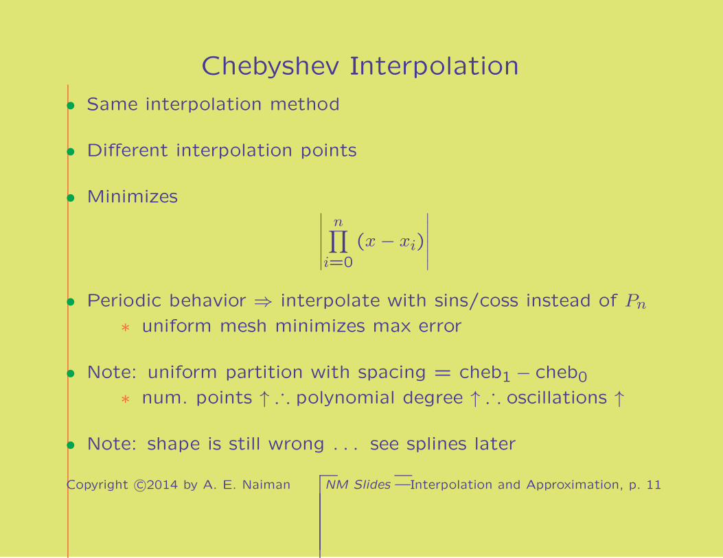
Chebyshev Interpolation

• Same interpolation method

• Different interpolation points

• Minimizes∣∣∣∣∣∣

n∏

i=0

(x− xi)

∣∣∣∣∣∣

• Periodic behavior ⇒ interpolate with sins/coss instead of Pn

∗ uniform mesh minimizes max error

• Note: uniform partition with spacing = cheb1 − cheb0∗ num. points ↑ · ·· polynomial degree ↑ · ·· oscillations ↑

• Note: shape is still wrong . . . see splines later




• Motivation


⇒ Numerical Differentiation




Numerical Differentiation

• Note: until now, approximating f(x), now f ′(x)

• f ′(x) ≈ f(x+h)−f(x)h

• Error = ?

• Taylor: f(x+ h) = f(x) + hf ′(x) + h2f ′′(ξ)2

• · ·· f ′(x) =f(x+ h)− f(x)

h− 1

2hf ′′(ξ)

• I.e., truncation error: O(h)

Can we do better?



Numerical Differentiation—Take Two

• Taylor for +h and −h:

f(x± h) =

f(x)± hf ′(x) + h2f′′(x)2! ± h3f

′′′(x)3! + h4f

(4)(x)4! ± h5f

(5)(x)5! + · · ·

• Subtracting:

f(x+ h)− f(x− h) = 2hf ′(x) + 2h3f ′′′(x)3!

+ 2h5f(5)(x)

5!+ · · ·

f ′(x) =f(x+ h)− f(x− h)

2h− 1

6h2f ′′′(x)− · · ·

• Note: for “=” there is either a ξ-term or “· · ·” — not both!

• Note: f(n)(ξ1) cannot cancel −f(n)(ξ2)We gained O(h) to O

(

h2)

. However, . . .



Richardson Extrapolation—Take Three

• We have

f ′(x) =f(x+ h)− f(x− h)

2h︸︷︷︸

≡φ(h)

+a2h2 + a4h

4 + a6h6 + · · ·

• Halving the stepsize, · ··

φ(h) = f ′(x)− a2h2 − a4h

4 − a6h6 − · · ·

φ

(h

2

)

= f ′(x)− a2

(h

2

)2

− a4

(h

2

)4

− a6

(h

2

)6

− · · ·

φ(h)− 4φ

(h

2

)

= −3f ′(x)− 3

4a4h

4 − 15

16a6h

6 − · · ·

Q: So what? A: The h2 term disappeared!



Richardson—Take Three (cont.)

• Divide by 3 and write f ′(x)

f ′(x) =4

3φ

(h

2

)

− 1

3φ(h)− 1

4a4h

4 − 5

16a6h

6 − · · ·

= φ

(h

2

)

+1

3

[

φ

(h

2

)

− φ(h)

]

︸︷︷︸

≡(∗)

+O(

h4)

• (∗) only uses old and current information

We gained O(

h2)

to O(

h4)

!!




• Motivation






Additional Notes• Three f ′(x) formulae used additional points ⇒

vs. Taylor, more derivatives in same point

• Similar for f ′′(x):

f(x± h) = f(x)±hf ′(x)+h2f ′′(x)2! ±h

3f′′′(x)3! +h4

f(4)(x)4! ±h

5f(5)(x)5! +· · ·

Adding:

f(x+ h) + f(x− h) = 2f(x) + h2f ′′(x) +1

12h4f(4)(x) + · · ·

or:

f ′′(x) =f(x+ h)− 2f(x) + f(x− h)

h2− 1

12h2f(4)(x) + · · ·

· ·· error = O(

h2)



Numerical Quadrature

⇒ Introduction

• Riemann Integration

• Composite Trapezoid Rule

• Composite Simpson’s Rule

• Gaussian Quadrature

Copyright c©2014 by A. E. Naiman NM Slides —Numerical Quadrature, p. 1


Numerical Quadrature—Interpretation

• f(x) ≥ 0 on [a, b] bounded ⇒ ∫ ba f(x) dx is area under f(x)

a b

function

value



Numerical Quadrature—Motivation

• Analytical solutions—rare:

∫ π2

0sinx dx = − cosx|

π20 = −(0− 1) = 1

• In general:∫ π

2

0

(

1− a2 sin2 θ)13 dθ

Need general numerical technique.



Lower Sum—Interpretation

x0 x1x2 x3x4

function

value

(= a) (= b)

Clearly a lower bound of integral estimate, and . . .



Upper Sum—Interpretation

x0 x1x2 x3x4

function

value

(= a) (= b)

. . . an upper bound. What is the max error?



Definitions• Mesh: P ≡ a = x0 < x1 < · · · < xn = b, n subintervals (n+1

points)

• Infima and suprema (or minima and maxima):

mi ≡ inf

f(x) : xi ≤ x ≤ xi+1

Mi ≡ sup

f(x) : xi ≤ x ≤ xi+1

• Two methods (i.e., integral estimates): lower and upper sums

L(f ;P) ≡n−1∑

i=0

mi

(

xi+1 − xi)

U(f ;P) ≡n−1∑

i=0

Mi

(

xi+1 − xi)

• Or combining, . . . . (how?)



Lower and Upper Sums—Example

• Third method, use lower and upper sums: (L+ U)/2

• f(x) = x2, [a, b] = [0,1] and P =

0, 14,12,

34,1

• . . . , L = 732, U = 15

32

• Split the difference: estimate 1132 (actual 1

3)

• Bottom line

∗ naive approach

∗ low n

∗ still error of 196. (!)

• Max error: (U − L)/2 = 18

Is this good enough?



Numerical Quadrature—Rethinking

• Perhaps lower and upper sums are enough?

∗ Error seems small

∗ Work seems small as well

• But: estimate of max error was not small (18)

• Do they converge to integral as n→∞?

• Will the extrema always be easy to calculate? Accurately?

(Probably not!)

Proceed in theoretical and practical directions.




• Introduction

⇒ Riemann Integration






Riemann Integrability

• f ∈ C0[a, b], [a, b] bdd ⇒ f is Riemann integrable

• When integrable, and max subinterval in P → 0 (|P |→0):

lim|P |→0

L(f ;P) =

∫ b

af(x) dx = lim

|P |→0U(f ;P)

• Counter example: Dirichlet function d(x) ≡

0, x rational,1, x irrational

⇒ L = 0, U = b− a



Challenge: Estimate n for Third Method

• Current restrictions for n estimate:

∗ Monotone functions

∗ Uniform partition

• Challenge:

∗ estimate

∫ π

0ecosx dx

∗ error tolerance = 12 × 10−3

∗ using L and U

∗ n = ?



Estimate n—Solution

• f(x) = ecos x ց on [0, π] · ·· mi = f(

xi+1

)

and Mi = f(xi)

• · ·· L(f ;P) = hn−1∑

i=0

f(

xi+1

)

and U(f ;P) = hn−1∑

i=0

f(xi), h = πn

• Want 12(U − L) < 1

2 × 10−3 or πn

(

e1 − e−1)

< 10−3

• . . . n ≥ 7385 (!!) (note for later: max error estimate = O(h))

• Number of f(x) evaluations

∗ 2 for (U − L) max error calculation

∗ > 7000 for either L or U

We need something better.




• Introduction


⇒ Composite Trapezoid Rule





Composite Trapezoid Rule—Interpretation

x0 x1x2 x3x4

function

value

(= a) (= b)

Almost always better than first three methods. (When not?)



Composite Trapezoid Rule (CTR)• Each area: 1

2

(

xi+1 − xi)[

f(xi) + f(

xi+1

)]

( CTR & CSR )

• Rule: T(f ;P) ≡ 1

2

n−1∑

i=0

(

xi+1 − xi)[

f(xi) + f(

xi+1

)]

• Note: for monotone functions and any given mesh (why?):

T = (L+ U)/2

• Pro: no need for extrema calculations

• Con: adding new points to existing ones (for a

non-monotonic function)

∗ T : “bad point” ⇒ ( last func., xi = −5,5, x2 = 0 )

no monotonic improvement (necessarily)

∗ L, U and (L+ U)/2 look for extrema on[

xi, xi+1

]

⇒monotonic improvement


http://demonstrations.wolfram.com/NumericalIntegrationUsingRectanglesTheTrapezoidalRuleOrSimps

http://demonstrations.wolfram.com/NumericalIntegrationUsingRectanglesTheTrapezoidalRuleOrSimps


Uniform Mesh and Associated Error

• Constant stepsize: h = b−an ,

nodes : x0 x1 x2 x3 · · · xn−1 xn

weights : 1↔ 1 1↔ 1 · · · 1 ↔ 1weights : 1↔ 1 1 · · · 1

total : 1 2 2 2 · · · 2 1

T(f ;P) ≡ h

n−1∑

i=1

f(xi) +1

2[f(x0) + f(xn)]

• Theorem: f ∈ C2[a, b] → ∃ξ ∈ (a, b) ∋−∫ b

af(x) dx− T(f ;P) = − 1

12(b− a)h2f ′′(ξ) = O

(

h2)

• Note: leads to popular Romberg algorithm (built on

Richardson extrapolation)

How many steps does T(f ;P) require?



ecos x Revisited—Using CTR

• Challenge:∫ π

0ecosx dx, error tolerance = 1

2 × 10−3, n = ?

• f(x) = ecos x ⇒ f ′(x) = −ecosx sinx . . .∣∣f ′′(x)

∣∣ ≤ e on (0, π)

• · ·· |error| ≤ 112π(π/n)

2e ≤ 12 × 10−3

• . . . n ≥ 119

• Recall perennial two questions/calculations of NM

∗ monotonic · ·· estimate of T produces same (L+ U)/2

∗ but previous max error estimate was less exact (O(h))

Better estimate of max error · ·· better estimate of n



Another CTR Example

• Challenge:

∫ 1

0e−x

2dx, error tolerance = 1

2 × 10−4, n = ?

• f(x) = e−x2, ⇒ f ′(x) = −2xe−x2 and f ′′(x) =

(

4x2 − 2)

e−x2

• · ··∣∣f ′′(x)

∣∣ ≤ 2 on (0,1)

• ⇒ |error| ≤ 16h

2 ≤ 12 × 10−4

• We have: n2 ≥ 13 × 104 or n ≥ 58 subintervals

How can we do better?




• Introduction



⇒ Composite Simpson’s Rule




Trapezoid Rule as∫

Linear Interpolant

Linear interpolant, one subinterval: p1(x) = x−ba−bf(a) +

x−ab−af(b),

intuitively:

∫ b

ap1(x) dx =

f(a)

a− b

∫ b

a(x− b) dx+

f(b)

b− a

∫ b

a(x− a) dx

=f(a)

a− b

[

b2 − a2

2− b(b− a)

]

+f(b)

b− a

[

b2 − a2

2− a(b− a)

]

= −f(a)[a+ b

2− b

]

+ f(b)

[a+ b

2− a

]

= −f(a)(a− b

2

)

+ f(b)

(b− a

2

)

=b− a

2(f(a) + f(b))

CTR is integral of composite linear interpolant.



CTR for Two Equal Subintervals

• n = 2 (i.e., 3 points):

T(f) =b− a

2

f

(a+ b

2

)

+1

2[f(a) + f(b)]

=b− a

4

[

f(a) + 2f

(a+ b

2

)

+ f(b)

]

with error = O

((b−a2

)3)

• (Previously, CTR error = O(

h2)

= TR error × n subintervals

= O(

h3)

×O(1h

)

)

• Deficiency: each subinterval ignores the other

How can we take the entire picture into account?



Simpson’s Rule

• Motivation: use p2(x) over the two equal subintervals

• Similar analysis actually loses O(h), but . . .

• Due to canceling terms, ∃ξ ∈ (a, b) ∋−

∫ b

af(x) dx =

b− a

6

[

f(a) + 4f

(a+ b

2

)

+ f(b)

]

− 1

90

(b− a

2

)5

f(4)(ξ)

• Similar to CTR, but weights midpoint more

• Note: for each method, denominator =∑

coefficients

Each method multiplies width by weighted average of height.



Composite Simpson’s Rule (CSR)• For an even number of subintervals n, h = b−a

n , ∃ξ ∈ (a, b) ∋−

• We have:

nodes : x0 x1 x2 x3 x4 x5 x6 · · · xn−2 xn−1 xn

weights : 1 4 1 1 4 1 · · · 1 4 1weights : 1 4 1 1 · · · 1

total : 1 4 2 4 2 4 2 · · · 2 4 1

∫ b

af(x) dx =

h

3

[f(a) + f(b)] + 4

n/2∑

i=1

f

a+ (2i− 1)h︸︷︷︸

odd nodes

+

2

(n−2)/2∑

i=1

f

a+2ih︸︷︷︸

even nodes

− b− a

180h4f(4)(ξ)

• Note: denominator =∑

coefficients = 3n

∗ but only n+1 function evaluations

• Pretty low error: Integration methods and more advanced

Can we do better than O(

h4)

?


http://demonstrations.wolfram.com/ComparingBasicNumericalIntegrationMethods

http://demonstrations.wolfram.com/NumericalIntegrationExamples


Integration Introspection• SR beat TR because heavier weighted midpoint

• But CSR, like CTR, suffers at subinterval-pair boundaries

(weight = 2 vs. 4 for no reason)

• All composite rules

∗ ignore other areas

∗ patch together local calculations

∗ · ·· will suffer from this

• Error: CTR: O(

h2f(2)(ξ))

, CSR: O(

h4f(4)(ξ))

• Note also, error = 0: CTR: ∀f ∈ P1, CSR: ∀f ∈ P3

• What about using all n+1 nodes and n-degree interpolation?

• Since error = 0, f ∈ Pn ⇒ lower error for general f?




• Introduction




⇒ Gaussian Quadrature



Interpolatory Quadrature

• xi, ℓi(x) =n∏

j = 0j 6= i

x− xj

xi − xj, i = 0, . . . , n; p(x) =

n∑

i=0

f(xi)ℓi(x)

• a = x0 and b = xn no longer required

•∫ b

ap(x) dx =

∫ b

a

n∑

i=0

f(xi)ℓi(x) dx =n∑

i=0

f(xi)∫ b

aℓi(x) dx

︸︷︷︸

≡Ai

• Ai = Ai

(

a, b;

xjn

j=0

)

, but Ai 6= Ai(f) !

• ∀f ∈ Pn ⇒ f(x) = p(x), and · ··

∀f ∈ Pn ⇒∫ b

af(x) dx =

n∑

i=0

Aif(xi), i.e., error = 0

(Endpoints, nodes) ⇒ Ai ⇒∫ b

af(x) dx ≈

n∑

i=0

Aif(xi).



Interp. Quad.—Error Analysis

• Uniform mesh: Newton-Cotes Quad. (TR: n = 1, SR: n = 2)

• Is

∫ b

af(x) dx ≈

∫ b

ap(x) dx ?

• Non-composite error: n even: O(

hn+3f(n+2)(ξ))

, n odd:

O(

hn+2f(n+1)(ξ))

• Often high order of h good enough, therefore popular

• What about Runge phenomenon: oscillations drive f(k) →∞?

• What if we choose n+1 specific nodes (with weights, total:

2(n+1) choices)?

Can we get error = 0 ∀f ∈ P2n+1?



Gaussian Quadrature (GQ)—Theorem

• Let

∗ q(x) ∈ Pn+1 ∋−∫ b

axkq(x) dx = 0, k = 0, . . . , n

i.e., q(x) ⊥ all polynomials of lower degree

∗ note: n+2 coefficients, n+1 conditions

⋆ unique to a constant multiplier

∗ xi, i = 0, . . . , n, ∋− q(xi) = 0

i.e., xi are zeros of q(x)

• Then ∀f ∈ P2n+1, even though f(x) 6= p(x) (∀f ∈ Pm, m > n)

∫ b

af(x) dx =

n∑

i=0

Aif(xi)

We jumped from Pn to P2n+1!



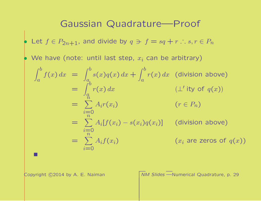
Gaussian Quadrature—Proof

• Let f ∈ P2n+1, and divide by q ∋− f = sq + r · ·· s, r ∈ Pn

• We have (note: until last step, xi can be arbitrary)

∫ b

af(x) dx =

∫ b

as(x)q(x) dx+

∫ b

ar(x) dx (division above)

=

∫ b

ar(x) dx

(⊥′ ity of q(x))

=n∑

i=0

Air(xi) (r ∈ Pn)

=n∑

i=0

Ai[f(xi)− s(xi)q(xi)] (division above)

=n∑

i=0

Aif(xi) (xi are zeros of q(x))



GQ—Additional Notes• Gaussian quadrature : 1) P2n+1 · ·· lower n with same

accuracy and fewer oscillations, 2) distr. like Chebyshev pts · ··tame oscillations

• Example qn(x): Legendre Polynomials: for [a, b] = [−1,1] and

qn(1) = 1 (∃ a 3-term recurrence formula, Legendre poly. )

q0(x) = 1, q1(x) = x, q2(x) =3

2x2 − 1

2, q3(x) =

5

2x3 − 3

2x, . . .

• Use qn+1(x) (why?), depends only on a, b and n

• Gaussian nodes ∈ (a, b)

∗ good if f(a) = ±∞ and/or f(b) = ±∞ (e.g.,

∫ 1

0

1√xdx)

• More general: with weight function w(x) in

∗ original integral

∗ q(x) orthogonality

∗ weights Ai


http://demonstrations.wolfram.com/GaussianQuadrature

http://demonstrations.wolfram.com/OrthogonalityOfTwoFunctionsWithWeightedInnerProducts


Numerical Quadrature—Summary

• n+1 function evaluations

composite? node placement error = 0 ∀PCTR

√uniform (usually)∗ 1

CSR√

uniform (usually)∗ 3

interp. × any (distinct) nGQ × zeros of q(x) 2n+1

∗P.S. There are also powerful adaptive quadrature methods



Linear Systems

⇒ Introduction

• Naive Gaussian Elimination

• Limitations

• Operation Counts


Copyright c©2014 by A. E. Naiman NM Slides —Linear Systems, p. 1


What Are Linear Systems (LS)?

a11 x1 + a12 x2 + · · · + a1n xn = b1a21 x1 + a22 x2 + · · · + a2n xn = b2

... + ... + .. . + ... = ...am1 x1 + am2 x2 + · · · + amn xn = bm

• Dependence on unknowns: powers of degree ≤ 1

• Summation form:n∑

j=1

ai j xj = bi , 1 ≤ i ≤ m, i.e., m

equations

• Presently: m = n, i.e., square systems (later: m 6= n)

Q: How to solve for [x1 x2 . . . xn]T? A: . . .



Linear Systems

• Introduction

⇒ Naive Gaussian Elimination

• Limitations





Overall Algorithm and Definitions

• Currently: direct methods only (later: iterative methods)

• General idea:

∗ Generate upper triangular system

(“forward elimination”)

∗ Easily calculate unknowns in reverse order

(“backward substitution”)

• “Pivot row” = current one being processed

“pivot” = diagonal element of pivot row

• “Naive” = no reordering of rows

Steps applied to RHS as well.



Forward Elimination

• Generate zero columns below diagonal

• Process rows downward

for each row i := 1, n− 1 // the pivot row

for each row k := i+1, n // ∀ rows below pivot

multiply pivot row ∋− ai i = ak i // “Gaussian multipliers”

subtract pivot row from rowk // now ak i = 0

// now column below ai i is zero

// now ai j = 0, ∀i > j

• Note: multiplication is temporary; pivot row is not changed

• Obtain triangular system

Let’s work an example, . . .



Compact Form of LS

6x1 − 2 x2 + 2 x3 + 4 x4 = 1612 x1 − 8 x2 + 6 x3 + 10 x4 = 263x1 − 13 x2 + 9 x3 + 3 x4 = −19

− 6x1 + 4 x2 + 1 x3 − 18 x4 = −34

→

6 −2 2 4 1612 −8 6 10 263 −13 9 3 −19−6 4 1 −18 −34

Proceeding with the forward elimination, . . .



Forward Elimination—Example

6 −2 2 4 1612 −8 6 10 263 −13 9 3 −19−6 4 1 −18 −34

−2R1

−12R1

−(−1)R1

→

6 −2 2 4 160 −4 2 2 −60 −12 8 1 −270 2 3 −14 −18

−3R2

−(

−12

)

R2

→

6 −2 2 4 160 −4 2 2 −60 0 2 −5 −90 0 4 −13 −21

−2R3

→

6 −2 2 4 160 −4 2 2 −60 0 2 −5 −90 0 0 −3 −3

Matrix is upper triangular.



Backward Substitution

6 −2 2 4 160 −4 2 2 −60 0 2 −5 −90 0 0 −3 −3

• Last equation: −3x4 = −3 ⇒ x4 = 1

• Second to last equation: 2x3 − 5 x4︸︷︷︸=1

= 2x3 − 5 = −9 ⇒

x3 = −2

• . . . second equation . . . x2 = . . .

• . . . [x1 x2 x3 x4]T = [3 1 − 2 1]T

For small problems, check solution in original system.



Linear Systems

• Introduction


⇒ Limitations





Zero Pivots

• Clearly, zero pivots prevent forward elimination

• ! zero pivots can appear along the way

• Later: When guaranteed no zero pivots?

• All pivots 6= 0?⇒ we are safe

Experiment with system with known solution.



Vandermonde Matrix

1 2 4 8 · · · 2n−1

1 3 9 27 · · · 3n−1

1 4 16 64 · · · 4n−1... ... ... ... . . . ...

1 n+1 (n+1)2 (n+1)3 · · · (n+1)n−1

• Want row sums on RHS ⇒ xi = 1, i = 1, . . . , n

• Geometric series:

1 + t+ t2 + · · ·+ tn−1 =tn − 1

t− 1

• We obtain bi, for row i = 1, . . . , n

n∑

j=1

(1 + i)j−1︸︷︷︸

ai j

· 1︸︷︷︸xj

=(1+ i)n − 1

(1+ i)− 1=

1

i[(1 + i)n − 1]

︸︷︷︸

bi

System is ready to be tested.



Vandermonde Test

• Platform with 7 significant (decimal) digits

∗ n = 1, . . . ,8 ⇒ expected results

∗ n = 9: error > 16,000% !!

• Questions:

∗ What happened?

∗ Why so sudden?

∗ Can anything be done?

• Answer: matrix is “ill-conditioned”

∗ Sensitivity to roundoff errors

∗ Leads to error propagation and magnification

First, how to assess vector errors.



Errors

• Given system: Ax = b and solution estimate x

• Residual (error): r ≡ Ax− b

• Absolute error (if x is known): e ≡ x− x

• Norm taken of r or e: vector → scalar quantity

(more on norms later)

• Relative errors: ||r||/||b|| and ||e||/||x||

Back to ill-conditioning, . . .



Ill-conditioning

• 0 · x1 + x2 = 1x1 + x2 = 2

⇒ 0 pivot

• General rule: if 0 is problematic ⇒numbers near 0 are problematic

• ǫ x1 + x2 = 1x1 + x2 = 2

. . . x2 =2−1/ǫ1−1/ǫ and x1 = 1−x2

ǫ

• ǫ small (e.g., ǫ = 10−9 with 8 significant digits) ⇒ x2 = 1 and

x1 = 0—wrong!

What can be done?



Pivoting

• Switch order of equations: non-Naive Gaussian Elimination

• Moving offending element off diagonal

• x1 + x2 = 2ǫ x1 + x2 = 1

⇒, x2 = 1−2ǫ1−ǫ and x1 = 2− x2 = 1

1−ǫ

• This is correct, even for small ǫ (or even ǫ = 0)

• Compare size of diagonal (pivot) elements above, to ǫ

• Ratio of first row of Vandermonde matrix = 1 : 2n−1

Issue is relative size, not absolute size.



Scaled Partial Pivoting

• Also called row pivoting (vs. column pivoting)

• Instability source: subtracting large values: ak j -= ai jak iai i

• W|o l.o.g.: n rows, and choosing which row to be first

• Find i ∋− ∀ rows k 6= i, ∀ columns j > 1: minimize∣∣∣ai j

ak 1ai1

∣∣∣

• O(

n3)

calculations! · ·· simplify (remove k), imagine: ak 1 = 1

• · ·· find i ∋− ∀ columns j > 1: mini

∣∣∣ai jai1

∣∣∣

• Still 1)O(

n2)

calculations, 2)how to minimize each row?

• Find i: minimaxj |ai j||ai1| , or: maxi

|ai1|maxj |ai j| (e.g., first matrix)



Linear Systems

• Introduction


• Limitations

⇒ Operation Counts




How Much Work on A?

• Real life: crowd estimation costs? (will depend on accuracy)

• Counting × and ÷ (i.e., long operations) only

• Pivoting: row decision amongst k rows = k ratios

• First row:

∗ n ratios (for choice of pivot row)

∗ n− 1 Gaussian multipliers

∗ (n− 1)2 multiplications

total: n2 operations

• · ·· forward elimination operations (for large n)

n∑

k=2

k2 =n

6(n+1)(2n+1)− 1 ≈ n3

3

How about the work on b?



Rest of the Work

• Forward elimination work on RHS:n∑

k=2

(k − 1) =n(n− 1)

2

• Backward substitution:n∑

k=1

k =n(n+1)

2

• Total: n2 operations

• O(n) fewer operations than forward elimination on A

• Important for multiple RHSs known from the start

∗ do not repeat O(

n3)

work for each

∗ rather, line them up, and process simultaneously

Can we do better at times?



Sparse Systems

× × 0 · · · · · · 0× × . . . . . . ...0 . . . . . .... . . . . . . ...

. . . 0... . . . . . . . . . ×0 · · · · · · 0 × ×

• Above, e.g., tridiagonal system (half bandwidth = 1)

∗ note: aij = 0 for |i− j| > 1

• Opportunities for savings

∗ storage

∗ computations

• Both are O(n)



Linear Systems

• Introduction


• Limitations





Pivot-Free Guarantee

• When are we guaranteed non-zero pivots?

• Diagonal dominance (just like it sounds):

|ai i| >n∑

j = 1j 6= i

∣∣∣ai j

∣∣∣, i = 1, . . . , n

• (Or “>” in one row, and “≥” in remaining)

• Many finite difference and finite element problems ⇒diagonally dominant systems

Occurs often enough to justify individual study.



LU Decomposition

• E.g.: same A, many b’s of time-dependent problem

∗ not all b’s are known from the start

• Want A = LU for decreased work later

• Then define y: L Ux︸︷︷︸≡y

= b

∗ solve Ly = b for y

∗ solve Ux = y for x

• U is upper triangular, result of Gaussian elimination

• L is unit lower triangular, 1’s on diagonal and Gaussian

multipliers below, e.g.:

1 0 0 02 1 0 0

1/2 3 1 0−1 −1/2 2 1

• For small systems, verify (even by hand): A = LU

Each new RHS is n2 work, instead of O(

n3)



Approximation by Splines

⇒ Motivation

• Linear Splines

• Quadratic Splines

• Cubic Splines

• Summary

Copyright c©2014 by A. E. Naiman NM Slides —Approximation by Splines, p. 1


Motivation

-40

-20

0

20

40

60

-4 -2 0 2 4

function

value

• ••

•

•

• Given: many points (e.g., n > 10), or very involved function

• Want: simple representative function for analysis or

manufacturing ( Designing a Car Body with Splines )

Any suggestions?


http://demonstrations.wolfram.com/DesigningACarBodyWithSplines


Let’s Try Interpolation

-40

-20

0

20

40

60

-4 -2 0 2 4

function

value

• ••

•

•

Disadvantages:

• Values outside x-range diverge quickly (interp(10) = −1592)

• Numerical instabilities of high-degree polynomials



Runge Function—Two Interpolations

0

1

c0c1c2c30x5x6x7x8

function

value

(= 5)(= x4 = c4)(= −5)

••••

•

••••

Chebyshevuniform

More disadvantages:

• Within x-range, often high oscillations

• Even Chebyshev points ⇒ often uncharacteristic oscillations

• Still high degree polynomial



Splines

Given domain [a, b], a spline S(x)

• Is defined on entire domain

• Provides a certain amount of smoothness

• ∃ partition of “knots” (= where spline can change form)

a = t0, t1, t2, . . . , tn = b

such that

S(x) =

S0(x), x ∈ [t0, t1],S1(x), x ∈ [t1, t2],

... ...Sn−1(x), x ∈ [tn−1, tn

]

is piecewise polynomial



Interpolatory Splines

• Note: splines split up range [a, b]

∗ opposite of CTR → CSR → GQ development

• “Spline” implies no interpolation, not even any y-values

• If given points

(t0, y0), (t1, y1), (t2, y2), . . . , (tn, yn)

“interpolatory spline” traverses these as well

Splines = nice, analytical functions




• Motivation

⇒ Linear Splines


• Cubic Splines

• Summary



Linear Splines

Given domain [a, b], a linear spline S(x)


• Provides continuity, i.e., is C0[a, b]

• ∃ partition of “knots”

a = t0, t1, t2, . . . , tn = b

such that

Si(x) = ai x+ bi ∈ P1

([

ti, ti+1

])

, i = 0, . . . , n− 1

Recall: no y-values or interpolation yet



Linear Spline—Examples

a b

function

value

undefined part

discontinuous

nonlinear part

linear spline

• Definition outside of [a, b] is arbitrary



Interpolatory Linear Splines

• Given points

(t0, y0), (t1, y1), (t2, y2), . . . , (tn, yn)

spline must interpolate as well

• Is S(x) (with no additional knots) unique?

∗ Coefficients: ai x+ bi, i = 0, . . . , n− 1 ⇒ total = 2n

∗ Conditions: 2 prescribed interpolation points for Si(x),

i = 0, . . . , n− 1 (includes continuity condition) ⇒total = 2n

• Obtain

Si(x) = ai x+ (yi − ai ti), ai =yi+1 − yi

ti+1 − ti, i = 0, . . . , n− 1



Interpolatory Linear Splines—Example

-40

-20

0

20

40

60

-4 -2 0 2 4

function

value

• •

•

•

•

Discontinuous derivatives at knots are unpleasing, . . .




• Motivation

• Linear Splines

⇒ Quadratic Splines

• Cubic Splines

• Summary



Quadratic Splines

Given domain [a, b], a quadratic spline S(x)


• Provides continuity of zeroth and first derivatives, i.e., is

C1[a, b]


a = t0, t1, t2, . . . , tn = b

such that

Si(x) = ai x2 + bi x+ ci ∈ P2

([

ti, ti+1

])

, i = 0, . . . , n− 1

Again no y-values or interpolation yet



Quadratic Spline—Example

f(x) =

x2, x ≤ 0,

−x2, 0 ≤ x ≤ 1,1− 2x, x ≥ 1,

f(x)?= quadratic spline

• Defined on domain (−∞,∞)√

• Continuity (clearly okay away from x = 0 and 1):

∗ Zeroth derivative:

⋆ f(

0−)

= f(

0+)

= 0

⋆ f(

1−)

= f(

1+)

= −1∗ First derivative:

⋆ f ′(

0−)

= f ′(

0+)

= 0

⋆ f ′(

1−)

= f ′(

1+)

= −2 √

• Each part of f(x) is ∈ P2√



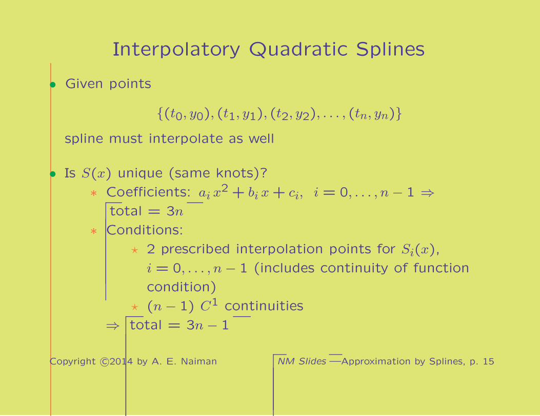
Interpolatory Quadratic Splines

• Given points

(t0, y0), (t1, y1), (t2, y2), . . . , (tn, yn)


• Is S(x) unique (same knots)?

∗ Coefficients: ai x2 + bi x+ ci, i = 0, . . . , n− 1 ⇒

total = 3n

∗ Conditions:

⋆ 2 prescribed interpolation points for Si(x),

i = 0, . . . , n− 1 (includes continuity of function

condition)

⋆ (n− 1) C1 continuities

⇒ total = 3n− 1



Interpolatory Quadratic Splines (cont.)

• Underdetermined system ⇒ need to add one condition

• Define (as yet to be determined) zi = S′(ti), i = 0, . . . , n

• Write

Si(x) =zi+1 − zi

2(

ti+1 − ti)(x− ti)

2 + zi(x− ti) + yi

therefore

S′i(x) =zi+1 − zi

ti+1 − ti(x− ti) + zi

• Need to

∗ verify continuity and interpolatory conditions

∗ determine zi



Checking Interpolatory Quadratic Splines

Check four continuity (and interpolatory) conditions:

(i) Si(ti)

√= yi

(ii) Si

(

ti+1

)

= (below)

(iii) S′i(ti)√= zi

(iv) S′i(

ti+1

)√= zi+1

(ii) Si

(

ti+1

)

=zi+1 − zi

2

(

ti+1 − ti)

+ zi(

ti+1 − ti)

+ yi

=zi+1 + zi

2

(

ti+1 − ti)

+ yi

set= yi+1

therefore (n equations, n+1 unknowns)

zi+1 = 2yi+1 − yi

ti+1 − ti− zi, i = 0, . . . , n− 1

Choose any 1 zi and the remaining n are determined.



Interpolatory Quadratic Splines—Example

-40

-20

0

20

40

60

-4 -2 0 2 4

function

value

• •

•

•

•

• •

•

•

•

z0 := 0

Okay, but discontinuous curvature at knots, . . .




• Motivation

• Linear Splines


⇒ Cubic Splines

• Summary



Cubic Splines

Given domain [a, b], a cubic spline S(x)


• Provides continuity of zeroth, first and second derivatives,

i.e., is C2[a, b]


a = t0, t1, t2, . . . , tn = b

such that for i = 0, . . . , n− 1

Si(x) = ai x3 + bi x

2 + ci x+ di ∈ P3

([

ti, ti+1

])

,

In general: spline of degree k . . . Ck−1 . . . Pk . . .



Why Stop at k = 3?

• Various orders of splines ; k too high ⇒ high oscillations

• Continuous curvature is visually pleasing

• Usually little numerical advantage to k > 3

• Technically, odd k’s are better for interpolating splines (later:

symmetric matrices and boundary conditions)

• Natural (defined later) cubic splines

∗ “best” in an analytical sense (stated later)


http://demonstrations.wolfram.com/InterpolatingASetOfData


Interpolatory Cubic Splines

• Given points

(t0, y0), (t1, y1), (t2, y2), . . . , (tn, yn)


• Is S(x) unique (same knots)?

∗ Coefficients: ai x3 + bi x

2 + ci x+ di, i = 0, . . . , n− 1 ⇒total = 4n

∗ Conditions:

⋆ 2 prescribed interpolation points for Si(x),

i = 0, . . . , n− 1 (includes continuity of function

condition)

⋆ (n− 1) C1 + (n− 1) C2 continuities

⇒ total = 4n− 2



Interpolatory Cubic Splines (cont.)

• Underdetermined system ⇒ need to add two conditions

• Natural cubic spline

∗ add: S′′(a) = S′′(b) = 0

∗ Assumes straight lines (i.e., no more constraints)

outside of [a, b]

∗ Imagine bent beam of Viking ship hull

∗ Defined for non-interpolatory case as well

• Required matrix calculation for Si definitions

∗ Linear: independent ai =yi+1−yiti+1−ti ⇒ diagonal

∗ Quadratic: two-term zi definition ⇒ bidiagonal

∗ Cubic: . . . ⇒ tridiagonal



Interp. Natural Cubic Splines—Example

-40

-20

0

20

40

60

-4 -2 0 2 4

function

value

• •

•

•

•

• •

•

•

•

Now the curvature is continuous as well. ( Cubic Spline )


http://demonstrations.wolfram.com/SimpleSplineCurves


Optimality of Natural Cubic Spline

• Theorem: If

∗ f ∈ C2[a, b],

∗ knots: a = t0, t1, t2, . . . , tn = b∗ interpolation points: (ti, yi) : yi = f(ti), i = 0, . . . , n

∗ S(x) is the natural cubic spline which interpolates f(x)

then∫ b

a

[

S′′(x)]2dx ≤

∫ b

a

[

f ′′(x)]2dx

• Bottom line

∗ average curvature of S ≤ that of f

∗ compare with interpolating polynomial




• Motivation

• Linear Splines


• Cubic Splines

⇒ Summary



Interpolation vs. Splines—Serpentine Curve

-2

-1.5

-1

-0.5

0

0.5

1

1.5

2

-2 -1.5 -1 -0.5 0 0.5 1 1.5 2

function

value

•• • • •

•••• • • •

•

interpolator

linear spline

Vs. oscillatory interpolator—even linear spline is better.



Three Splines

-20

0

20

40

60

80

-4 -2 0 2 4

function

value

• •

•

•

•

• •

•

•

•

linear

quadratic

natural cubic

Increased smoothness with increase of degree.



Ordinary Differential Equations

⇒ Introduction

• Euler Method

• Higher Order Taylor Methods

• Runge-Kutta Methods

• Summary

Copyright c©2014 by A. E. Naiman NM Slides —Ordinary Differential Equations, p. 1


Ordinary Differential Equation—Definition• ODE = an equation

∗ involving one or more derivatives of x(t)

∗ x(t) is unknown and the desired target

∗ somewhat opposite of numerical differentiation

• E.g.:(

x′′′)37(t) + 37 t ex

2(t) sin 4√

x′(t)− log 1t = 42 ⇒

Which x(t)’s fulfill this behavior?

• “Ordinary” (vs. “partial”) = one independent variable t

• “Order” = highest (composition of) derivative(s) involved

• “Linear” = derivatives, including zeroth, appear in linear form

• “Homogeneous” = all terms involve some derivative

(including zeroth)



Analytical Approach

• Good luck with previous equation, but others . . .

• Shorthand: x = x(t), x′ = d(x(t))dt , x′′ = d2(x(t))

dt2, . . .

• Analytically solvable∗ x′ − x = et ⇒ x(t) = t et + c et

∗ x′′+9x = 0 ⇒ x(t) = c1 sin 3t+ c2 cos 3t

∗ x′+ 12x = 0 ⇒ x(t) =

√c− t

• c, c1 and c2 are arbitrary constants

• Need more conditions/information to pin down constants

∗ Initial value problems (IVP)

∗ Boundary value problems (BVP)

Here: IVP for first-order ODE.



First-Order IVP

• General form:

x′ = f(t, x), x(a) given

• Note: non-linear, non-homogeneous; but, x′ not on RHS

• Examples∗ x′ = x+1, x(0) = 0 ⇒ x(t) = et − 1

∗ x′ = 6t− 1, x(1) = 6 ⇒ x(t) = 3t2 − t+4

∗ x′ = tx+1, x(0) = 0 ⇒ x(t) =

√

t2 +1− 1

• Physically: e.g., t is time, x is distance and f = x′ isspeed/velocity

Another optimistic scenario . . .



RHS Independence of x

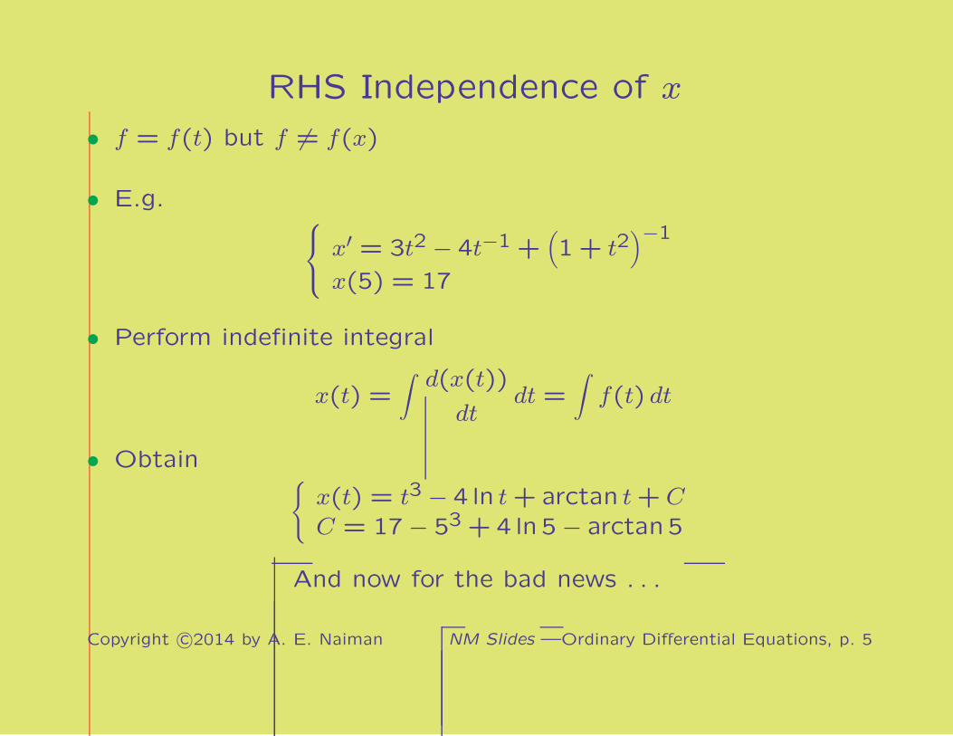
• f = f(t) but f 6= f(x)

• E.g.

x′ = 3t2 − 4t−1 +(

1 + t2)−1

x(5) = 17

• Perform indefinite integral

x(t) =∫

d(x(t))

dtdt =

∫

f(t) dt

• Obtain

x(t) = t3 − 4 ln t+arctan t+ C

C = 17− 53 +4 ln5− arctan5

And now for the bad news . . .



Numerical Techniques

• Source of need

∗ Usually analytical solution is not known

∗ Even if known, perhaps very complicated, expensive to

compute

• Numerical techniques

∗ Generate a table of values for x(t)

∗ Usually equispaced in t, stepsize = h

∗ ! with too small h, and far from initial value

roundoff error can accumulate and kill

How do we step from x(t) to x(t+ h)?



Differential Equations and Integration• Close connection between the two, with similar techniques

• Consider (τ is a time variable):

dxdτ = f(τ, x)x(a) = s

• Multiply by dτ and integrate from t to t+ h:∫ t+h

tdx =

∫ t+h

tf(τ, x(τ))dτ

• Therefore:

x(t+ h) = x(t) +∫ t+h

tf(τ, x(τ))dτ

• We can—and will!—replace integral with previous numerical

techniques



Practical Example — F = ma

• Newton’s second law of motion

• Rocket fired vertically, with displacement x and velocity v

• With just gravity (981) ⇒ solve analytically

• Propulsion upwards: 5370 (with correct units)

• Negative force of air resistance: v3/2/ ln (2 + v)

• Decrease in mass (m = m(t)) due to fuel burn: 321− 24t;

fuel gone by t = 10 seconds

5370− 981− v3/2/ ln (2 + v) = (321− 24t)v′

What is v(10)?




• Introduction

⇒ Euler Method



• Summary



Euler Method—Example (t sin t on [1.2,3])

x(a

)

a

function

value,x(t)

t

••

• • ••

•

•

h

actual function

Euler*

-

• explicit Euler ; when will the slopes match up at the points?

Okay, but not great. What about accuracy?


http://demonstrations.wolfram.com/NumericalMethodsForDifferentialEquations


Euler Method

• First-order IVP: given x′ = f(t, x), x(a), want x(b)

• Use first 2 terms of Taylor series (i.e., n = 1) to get from

x(a) to x(a+ h)

x(a+ h) = x(a) + hx′(a)︸︷︷︸

use f(a, x(a))

+

truncation error︷︸︸︷

O(

h2)

• This is just the left rectangle approximation of the integral

• Repeat to get from x(a+ h) to x(a+2h), . . .

• Total n = b−ah steps until x(b)

• Note: units of time/distance/speed are consistent



Euler Method—Pros and Cons

• Note: straight lines connecting points

∗ from Euler construction (linear in h)

∗ can be used for subsequent linear interpolation

• Advantages

∗ Accurate early on: O(

h2)

for first step

∗ Only need to calculate given function f(t, x(t))

∗ Only one evaluation of f(t, x(t)) needed

• Disadvantages

∗ Pretty inaccurate at b

∗ Cumulative truncation error: n×O(

h2)

= O(h)

∗ This is aside from (accumulative) roundoff error

How about more terms of the Taylor series?




• Introduction

• Euler Method

⇒ Higher Order Taylor Methods


• Summary



Taylor Method of Order 4

• First-order IVP: given x′ = f(t, x), x(a), want x(b)

• Use first 5 terms of Taylor series (i.e., n = 4) to get from

x(a) to x(a+ h)

x(a+ h) = x(a)+hx′(a)︸︷︷︸

use f(a, x(a))

+h2

2!x′′(a)+

h3

3!x′′′(a)+

h4

4!x(iv)(a)+O

(

h5)

• Use f ′, f ′′ and f ′′′ for x′′, x′′′ and x(iv), respectively

• Repeat to get from x(a+ h) to x(a+2h), . . .

• Note: units of time/distance/speed still are consistent

Order 4 is a standard order used.



Taylor Method—Numerical Example

• First-order IVP: x′ = 1+ x2 + t3, x(1) = −4, want x(2)

• Derivatives of f(t, x)

x′′ = 2x x′+3t2

x′′′ = 2x x′′+2(

x′)2

+6t

x(iv) = 2x x′′′+6x′ x′′+6

• Solution values of x(2), n = 100

∗ actual: 4.3712 (5 significant digits)

∗ Euler: 4.2358541

∗ Taylor4: 4.3712096

How about the earlier graphed example?



Taylor Method of Order 4—Example

x(a

)

a

function

value,x(t)

t

••

• • ••

•

•

h

actual function

Euler

Taylor4

*

:

-

Single step truncation error of O(

h5)

⇒ excellent match.



Taylor Method of Order 4—Larger Step

x(a

)

a

function

value,x(t)

t

••

• • ••

•

•

h

actual function

Euler

Taylor4, h→ 7h

*

z

-

Even single Taylor4 step beats Euler.



Taylor Method—Pros and Cons

• Note: graphs connecting points: from construction (P4 in h)

• Advantages

∗ Very accurate

∗ Cumulative truncation error: n×O(

h5)

= O(

h4)

• Disadvantages

∗ Need derivatives of f(t, x(t)) which might be

⋆ analytically: difficult

⋆ numerically: expensive—computationally and/or

accuracy-wise

⋆ just plain impossible

∗ Four new evaluations each step (Euler was just one)

How to avoid the extra derivatives?




• Introduction

• Euler Method


⇒ Runge-Kutta Methods

• Summary



Motivation

• We want to avoid calculating derivatives of f(t, x(t))

• Similar to Newton→secant motivation

• Also, recall different approaches for higher accuracy

∗ Taylor series: more derivatives at one point

∗ Numerical differentiation: more function evaluations, at

various points

• Runge-Kutta (RK) of order m: for each step of size h

∗ evaluate f(t, x(t)) at m interim stages

∗ arrive at accuracy order similar to Taylor method of

order m



Runge-Kutta Methods: RK2 and RK4• Each f(t, x(t)) evaluation builds on previous

• Weighted average of evaluations produces x(t+ h)

• Error for order m is O(

hm+1)

for each step of size h

• Note: units of time/distance/speed—okay

RK2:

x(t+ h) = x(t) + 12(F1 + F2)

F1 = hf(t, x)F2 = hf(t+ h, x+ F1)

RK4:

x(t+ h) = x(t)+16(F1 +2F2 +2F3 + F4)

F1 = hf(t, x)

F2 = hf(

t+ 12h, x+ 1

2F1

)

F3 = hf(

t+ 12h, x+ 1

2F2

)

F4 = hf(t+ h, x+ F3)



RK2 Derivation

• Trapezoid rule:

∫ t+h

tf(τ, x(τ))dτ ≈ h

2[f(t, x(t)) + f(t+ h, x(t+ h))]

• Our formula now:

x(t+ h) = x(t) +h

2[f(t, x(t)) + f(t+ h, x(t+ h))]

• Since x(t+ h) on both sides ⇒ “implicit” formula

• With Euler (which is “explicit”):

x(t+ h) = x(t) + hf(t, x(t))

on RHS, we have RK2




• Introduction

• Euler Method



⇒ Summary



Summary—First-Order IVP Solvers• Complex and complicated IVPs require numerical methods

• Usually generate table of values, at constant stepsize h

• Euler: simple, but not too accurate

• High-order Taylor: very accurate, but requires derivatives of

f(t, x(t))

• Runge-Kutta: same order of accuracy as Taylor, without

derivative evaluations

• Error sources

∗ Local truncation (of Taylor series approximation)

∗ Local roundoff (due to finite precision)

∗ Accumulations and combinations of previous two



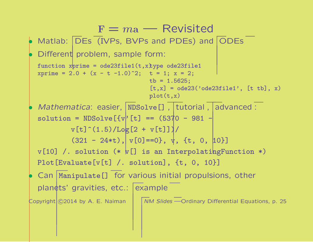
F = ma — Revisited• Matlab: DEs (IVPs, BVPs and PDEs) and ODEs

• Different problem, sample form:

function xprime = ode23file1(t,x)xprime = 2.0 + (x - t -1.0)^2;

type ode23file1t = 1; x = 2;tb = 1.5625;[t,x] = ode23(’ode23file1’, [t tb], x)plot(t,x)

• Mathematica: easier, NDSolve[] , tutorial , advanced :

solution = NDSolve[v’[t] == (5370 - 981 -

v[t]^(1.5)/Log[2 + v[t]])/

(321 - 24*t), v[0]==0, v, t, 0, 10]

v[10] /. solution (* v[] is an InterpolatingFunction *)

Plot[Evaluate[v[t] /. solution], t, 0, 10]

• Can Manipulate[] for various initial propulsions, other

planets’ gravities, etc.: example


http://www.mathworks.com/products/matlab/examples.html?file=/products/demos/shipping/matlab/odedemo.html

http://www.mathworks.com/help/matlab/math/ordinary-differential-equations.html;jsessionid=db467b57484992746463a203518a?s_tid=doc_12b

http://reference.wolfram.com/mathematica/ref/NDSolve.html

http://reference.wolfram.com/mathematica/tutorial/NumericalSolutionOfDifferentialEquations.html

http://reference.wolfram.com/mathematica/tutorial/NDSolveOverview.html

http://reference.wolfram.com/mathematica/ref/Manipulate.html

http://jct.ac.il/~naiman/nm/manip-ode.nb


Least Squares Method

⇒ Motivation and Approach

• Linearly Dependent Data

• General Basis Functions

• Polynomial Regression

• Function Approximation

Copyright c©2014 by A. E. Naiman NM Slides —Least Squares Method, p. 1


Source of Data

• Have the following tabulated data:x x0 x1 · · · xmy y0 y1 · · · ym

yivalues

xi values

•• •

••• • •

• •

• E.g., data from experiment

• Assume known dependence, e.g. linear, i.e., y = ax+ b

What a and b do we choose to represent the data?



Most Probable Line

• For each point, consider the equation yi = axi + b with the

two unknowns a and b

• One point ⇒ ∞ solutions

• Two points (different xi) ⇒ one unique solution

• > two points ⇒ in general no solution

> two points ⇒ What is most probable line?



Estimate Error

• Assume estimates a and b ⇒error at (xk, yk): ek = axk + b− yk

yivalues

xi values

•• •

••• • •

• •(xk, yk)

height is ek

y = ax+ b

• Note:

∗ vertical error, not distance to line (a much harder

problem)

∗ |ek| ⇒ no preference to error direction

How do we minimize all of the |ek|?



Vector Minimizations

Minimize:

• largest component: mina,b

max0≤k≤m

|ek|, “min-max”

• component sum: mina,b

m∑

k=0

|ek|, linear programming

Note: |·| won’t allow errors to cancel

• component squared sum: mina,b

m∑

k=0

e2k︸︷︷︸

≡φ(a,b)

, least squares

Why use least squares?



ℓp Norms

• Definition: ||v||p ≡

m∑

k=0

|vk|p

1p

, p-Norms (Norm[]→Abs[x]. . .)

• Minimizing ℓ∞, ℓ1 and ℓ2 norms, resp., in 2–D (m = 1):

-

6

v0

v1

1

1

−1

−1

||v||∞ = 1

||v||∞ = max(|v0|, |v1|)

7

v

-

6

v0

v1

1

1

−1

−1

||v||1 = 1

||v||1 = |v0|+ |v1|

7

v-

6

v0

v1

1

1

−1

−1

||v||2 = 1

||v||2 =√

v20 + v21

7

v

• Why use ℓ2?

∗ Can more easily use calculus (see below)

∗ If error is normally distributed ⇒get maximum likelihood estimator


http://demonstrations.wolfram.com/UnitNormVectorsUnderDifferentPNorms


φ(a, b) Minimization

• How do we minimize φ(a, b) =m∑

k=0

e2k wrt a and b?

• Standard calculus:∂φ

∂a

set= 0 and

∂φ

∂b

set= 0 ⇒

two equations with two unknowns

• If dependence of y on a and b is linear (and consequently,

dependence of φ(a, b) is quadratic) ⇒minimization leads to linear system for a and b

(linear least squares)

• Example also had linearly dependent data, i.e., y linear in x

• Non-linear LS, e.g.: a sin b x+ c cos d x, aeb x + ce−d x

Minimization of our example, . . .




• Motivation and Approach

⇒ Linearly Dependent Data






LLS for Linearly Dependent Data—Method

Function to minimize:

φ(a, b) =m∑

k=0

e2k =m∑

k=0

(axk + b− yk)2

lead to two differentiations:

2m∑

k=0

(axk + b− yk)xk = 0, and 2m∑

k=0

(axk + b− yk) = 0

or as a system of linear equations in a and b:

m∑

k=0

x2k

a +

m∑

k=0

xk

b =

m∑

k=0

xk yk

m∑

k=0

xk

a + (m+1)b =

m∑

k=0

yk

Coefficient matrix = cross-products of a and b coefficients.



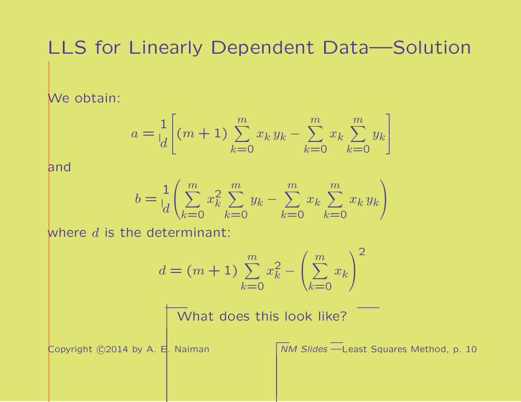
LLS for Linearly Dependent Data—Solution

We obtain:

a =1

d

(m+1)m∑

k=0

xk yk −m∑

k=0

xk

m∑

k=0

yk

and

b =1

d

m∑

k=0

x2k

m∑

k=0

yk −m∑

k=0

xk

m∑

k=0

xk yk

where d is the determinant:

d = (m+1)m∑

k=0

x2k −

m∑

k=0

xk

2

What does this look like?



LLS Solution for Sample Data

yivalues

xi values

•

• •

••

• ••• •

What about non-linearly dependent data?






⇒ General Basis Functions





Non-Linearly Dependent Data

• Linear least squares—for linear combination of any functions,

e.g.:

y = a ln x+ b cosx+ cex

• Minimization of φ: three differentiations:

∂φ

∂a

set= 0,

∂φ

∂b

set= 0 and

∂φ

∂c

set= 0

• Elements of matrix: sums of cross-products of functions:

m∑

k=0

lnxk exk,

m∑

k=0

(cos xk)2, . . .

A more general form, . . .



Linear Combinations of General Functions• m+1 points (x0, y0), (x1, y1), . . . , (xm, ym)

• n+1 “basis” functions g0, g1, . . . , gn, such that

g(x) =n∑

j=0

cj gj(x)

• Error function φ

φ(c0, c1, . . . , cn) =m∑

k=0

n∑

j=0

cj gj(xk)− yk

2

• Minimization:

∂φ

∂ci= 2

m∑

k=0

n∑

j=0

cj gj(xk)− yk

gi(xk)set= 0, i = 0, . . . , n

Pulling it together, . . .



Normal Equations• “Normal equations”:

n∑

j=0

m∑

k=0

gi(xk) gj(xk)

cj =m∑

k=0

yk gi(xk), i = 0, . . . , n

• Note: n+1 equations (i.e., rows) and n+1 columns

• (Coefficient matrix)i j =m∑

k=0

gi(xk) gj(xk)

• Possible solution method: Gaussian elimination

• Require of gj(x) for any solution method

∗ linear independence (lest there be no solution)

∗ appropriateness (e.g., not sin’s for linear data)

∗ well-conditioned matrix (opposite of ill-conditioned)



Choice of Basis Functions

• What if basis functions are unknown?

• Choose them for numerically “good” coefficient matrix (at

least not ill-conditioned)

• Orthogonality ⇒ diagonal matrix, would be nice

• Orthonormality ⇒ identity matrix, would be best, i.e.,m∑

k=0

gi(xk) gj(xk) = δi j and compute coefficients directly

ci =m∑

k=0

yk gi(xk), i = 0, . . . , n

• Can be done with Gram-Schmidt process

Another method for choosing basis functions, . . .



Chebyshev Polynomials

• Assume that the basis functions are ∈ Pn, xi ∈ [−1,1]

• 1, x, x2, x3, . . . are too alike to describe varying behavior

• Use Chebyshev polynomials: 1, x,2x2 − 1,4x3 − 3x, . . .

-1

1

0 0.2 0.4 0.6 0.8 1

function

value

xjT1

T2

T3

T4T5

. . . with Gaussian elimination produces accurate results.







⇒ Polynomial Regression




Motivation and Definition

• Want to smooth out data to a polynomial pN(x) —

play online! :-)

• Problem: what degree N polynomial? Curve Fitting

• For m+1 points, certainly N < m, as N = m is interpolation

• Define variance σ2n

σ2n =1

m− n

m∑

k=0

[yk − pn(xk)]2 (n < m)

• Note: summation part (i.e., without leading fraction) of σ2n∗ is monotonic non-increasing with n (why?)


http://demonstrations.wolfram.com/LinearAndQuadraticCurveFittingPractice

http://demonstrations.wolfram.com/CurveFitting


Regression Theory

• Statistical theory: if data (with noise) is really of pN(x), then:

σ20 > σ21 > σ22 > · · · > σ2N ≈ σ2N+1 ≈ σ2N+2 ≈ · · · ≈ σ2m−1

• · ·· with reasonable noise, stop when σ2N ≈ σ2N+1 ≈ σ2N+2 ≈ · · ·

σ2N

N − 4 N N +4

σ2 n

polynomial degree, n

•

•• • • • • • • • •








⇒ Function Approximation



Continuous Data

• Given f(x) on [a, b], perhaps from experiment

• Replace complicated or numerically expensive f(x) with

g(x) =n∑

j=0

cj gj(x)

• Continuous analog of error function

φ(c0, c1, . . . , cn) =

∫ b

a[g(x)− f(x)]2dx

• Can also weight parts of the interval differently

φ(c0, c1, . . . , cn) =

∫ b

a[g(x)− f(x)]2w(x) dx



Normal Equations and Basis Functions

• Differentiating, we get the normal equations

n∑

j=0

[∫ b

agi(x) gj(x)w(x) dx

]

cj =∫ b

af(x) gi(x)w(x) dx, i = 0, . . . , n

• Want orthogonality of (coefficient matrix)i j

∫ b

agi(x) gj(x)w(x) dx = 0, i 6= j

• For weighting interval ends, use Chebyshev polynomials

( Chebyshev poly. ) since

∫ 1

−1Ti(x)Tj(x)

1√

1− x2dx =

0, i 6= j,π2, i = j > 0

π, i = j = 0


http://demonstrations.wolfram.com/OrthogonalityOfTwoFunctionsWithWeightedInnerProducts


A Nonlinear Case

• Start with same tabulated data:x x0 x1 · · · xmy y0 y1 · · · ym

• But the functional dependence is nonlinear, e.g.: y = ec x

• Similarly as before, the function to minimize:

φ(c) =m∑

k=0

(ec xk − yk)2

• However, differenting and equating to zero:

dφ

dc= 2

m∑

k=0

(ec xk − yk)ec xkxk

set= 0

is highly nonlinear

• One possibility: methods (Newton, secant, etc.) for roots of

this nonlinear equation

• Another: minimization techniques for φ(x) itself



Approximating by Linearization• Another approach: transform nonlinear problem to linear one

• Define: z ≡ c x, then for y = ec x, we have: z = ln y

• We now define a different minimization (in “ln space”):

φ(c) =m∑

k=0

(c xk − zk)2 (zk ≡ ln yk)

• This leads to a simple, linear equation in c:

c =

m∑

k=0

zkxk

m∑

k=0

x2k

• Minimal noise : c ≈ c; no noise: c = c


http://jct.ac.il/~naiman/nm/nonlinear-ls.nb


Linear/Nonlinear Example• Same data: (xk, yk), k = 0, . . . ,m

• Functional dependence: y = a sin (b x)

• Note: linear in a and nonlinear in b

• Function to minimize:

φ(a, b) =m∑

k=0

(a sin (b xk)− yk)2

• Differentiating and setting to zero:

m∑

k=0

[a sin (b xk)− yk] sin (b xk) = 0

m∑

k=0

[a sin (b xk)− yk]a xk cos (b xk) = 0



Linear/Nonlinear Example (cont.)

• If b known ⇒ we get a from either equation:

a =

m∑

k=0

yk sin (b xk)

m∑

k=0

[sin (b xk)]2

, and a =

m∑

k=0

xkyk cos (b xk)

m∑

k=0

xk sin (b xk) cos (b xk)

• Need to find b such that the two forms are equal

• Possible methods: bisection, Newton, secant, etc.



Motivation

• Typical problem: traffic lights (sans clover leaf)

∗ given traffic flow parameters . . .

∗ how to determine the optimal period

∗ how to distribute the time per period

∗ note: these are all inter-dependent

• Analytically very hard (or impossible)

• Empirical simulation can approach the problem

• Need to implement randomization for modeling various

conditions

Less mathematical, but not less important.



Random Numbers—Usage

• With simulation ⇒ assist understanding of

∗ standard/steady state conditions

∗ various perturbations

• Monte Carlo: running a process many times with

randomization

∗ help draw statistics



Random Numbers—Requirements

• Not ordered, e.g., monotonic or other patterns

• Equal distribution

• Often RNG produce x ∈ [0,1)

• Desired (demanded!): P(a, a+ h) = h; independent of a

• Low or no periodicity

• No easy generating function from one number to the next

∗ can be deceivingly random-looking

∗ e.g.: digits of π



Random Number Generators

• Computers are deterministic ⇒ not an easy problem

• Current computer 1100 of seconds—not good

∗ for requests every < 1100 second

∗ for any requests with periodicity of 1100 second

• Often based on Mersenne primes ( Mersenne primes )

∗ so far, 48 of them

∗ definition: 2k − 1, for some k

∗ e.g.: k = 31 ⇒ 2,147,483,647

∗ largest (as of 2/2013): k = 57,885,161 ⇒ 17,425,170

decimal digits!

∗ other usages: cryptology


http://en.wikipedia.org/wiki/Mersenne_prime


Testing and Using a RNG

• “Not all RNG were created equal!”

• One can (and should) histogram a RNG

• Not obvious (nor necessarily known)

∗ number of trials necessary for testing a RNG

∗ number of trials necessary when using a RNG

• Require better RNG, for higher usage of RNG

• For ranges other than [0,1): apply obvious mapping



Incorrect Usage—In an Ellipse

-1

-0.5

0

0.5

1

-2 -1 0 1 2

function

value

+

++

+

+

+

+

+

+

+

++

+

+

+

+

+ ++

+

+

+

+

+

+

+

+

++

+

+

+++

+

+

++

+

++

+

+

+

+

+

+

+

+

+

+

+ +

++

++

+

+

+

+

+

++

+

+

+

+

+

+

+

+

+

+

+

+

+

++ +

+

++

+ +

+

++

+

++

++

+

+

+

+

+

+

+

+

++

++

+

+

+++

+

+

+

+

+

+

+

++

+

++

+

+

+

+

+

+

+

++

+

+

+

+

+

++

+

++

+

+

++

+

+

+

+

+

+

+

+

++

+

+

++

+

+

+

+

+

+

+

+

+

+

+

+

+

+

+

++

++

+

+

+

+

+

+

+

+

+

++

+

+

+

+

+

++

+

+

+

+

+

+

+

+

+

+

++

+

++

++

++

+

+

+

+

+

+

++

+

+

+

+

+

+

+

++

++

++

+

+

+

++

+

++

++

+

+

+

+

+

+

+

+

+

+

+

+

+

+

+

+ +

++

+

+

++

+

+

+

+

+

+

+

+

+

+

+

++

+

+

+

+

+

+

+

++

+

+

+

+

+

+

+

++

+

+

+

+

++

+++

+

+

+

+

++

+

+

+

+

+

+

+

+

++

++

+

+

+

+

++

+

+

+

+++ +

+

+

+

+ +++

++

+

++

+++

++

+

+

++

+

+

+

+

+

+

+

+

+

+

+

+

+

+

+

+

+

+

+

++

+

+

+

++

+

+ +

+

+

+

+

++++

+

+

+

+

+

+

+

+

++

+

+

+

+

+

+

+

+

+

+

+

++

+

+ +

+

+

++

+ +

+

+

++

++

+

++

+

+

+

+

+

+ ++

+

+

+

++

+

+

++

+

+

+

+

+ +

+

++

+

+

+

+

+

+

+

++

+

++

+

+

++

+

+

+

+

++

+

+ +

+

+

+

+

+

++

+

+

+

+

+

+

+

+

+

+

+

+

+

+

+

+

++

++

+

+

+

+

+

+

+

+

++

+ +

+

+

+

+

++

+

+

+

+

+

+

++

+

+

+

++

+

+

+

+

+

+

+

+

+

+

++

+

+

+

+

++

+

++

+

+

+

++

+

+

+ +

++

+

+

+ +

+

+

+

+

++

+

+

++

+

++

+

+

+

++ +

+

+

+ ++

+

+

+

++

+

+

+

+

+

+

+

++

+

++

+

++

+

+

++

+

+

+

+ +

+ +

+

+

+

+

+

+

+

++

+

+

+

++

+

+

+

+

+

+

+

+

+

+

+

+

+

++

+

+

+

+

++

++

+

+

+

+

+

++

+ +

+

+ +

+

++

+

+

+

+

++

+

+

+++

+

++

+ +

++

+

+

+

+

+

+ +

+

++

+

+

+

+

+

+

+

+

+

+

+

++

+

+

+++

+

+

+

+

+

+

+

+ +

++

+

+

+

+

+

+

+

+

+

+

+

+

+

++

+

+

+

+

+

+

++

+

+

++

+ ++

+

+

+

+

+

+

+

+

+

+

+

+

+

+

+

+

++ +

+

+

+

+

+

+++

+

+

+

+

+

+

+

+

+

+

+

+

+

+

+

++ +

+

+

+

++

+

++

+

+

+

+

+

+

+ +++

++

+

+

+

+

+

+

+

+

+

+

+

++

++

+

+

+

+

+

+

++

+

+

+

+

+

+

++

+ +

+

+

+

++

+

+

+

+

+

+

+

+

+

+

+

++

+

+

+

++

+

+

+

+

+

+

+

+

++

+

+

+

+

++ +

+

+

+

+

+

+

+

+++ +

+

++

+

+++

+

+

+

+

+

+++ +

+++

+

+

+

+

+

+ +

+

+

+

+

+

+

+++

++

+

+

+

++

+

++

+

+ +

++

+

+

+

+

++

+

+

++

+

+

+ +

+

+

+

+

++

+

+

+

• Equation: x2 +4y2 = 4

• Generation algorithm:

∗ xi ∈ rng(−2,2), yi ∈ rng(−1,1)∗ yi correction: yi← (yi/2)

√

4− x2i

Points bunch up at ends ⇒ non-uniformity.



Incorrect Usage—In a Circle

-1

-0.5

0

0.5

1

-1 -0.5 0 0.5 1

function

value

++

+

+++

+

+

+

+

+

+

+

+

+

+

+ +

+

+

+

+

+

+

+

+

+

+

+

+

+

+

+

+

+

+

++

+

+

++

+

+

+

+

+

+

+

+

++

++

+

+

+

+

+

+

+

+

+

+

+

+

+

+

+

+++

+

+

+

+

+

+

++

+

+

+

+

++ +

+

+

+

+

+

+

+

+

+

+

+

+

+

+++

+

+

+

+

+

++

+

+

+

+

++

+

+

+

+

++

+

++

+

+

+

+

+

+

+

+

+

+

+

++

+

+

+

+

+

+

+

+

+

+ ++

+

+

+

+++

+

+

+

+

+

+

+

+

+++

+

++

+

+

+

+

+

++

++

+

+

+

+

+

++

+

+

+

+

+

+

+

+

+

+

+

+

+

+

+

+

+

++

+

+

+

+

+

+

+

+

++

+

+

+

+

++

++

+

+

+

+

+

+

+

+

++

++

+

+

+

+ +

+

+

+

+

+

+

++

+

+

+

+

+

++

++

+

++

++

+

+

+

+

+

++

+

+

+

+

+

+

+

+

+

+

+

+

+

+

+

+

+

+

+

+

++

+

+

++

+

+

+

++

+

+

+

+

+

+

+

++

+

+

+

+

++

+

+

+

+

+

+

+

+

+

+

++

+

+

+

+

+

+

++

++

++

+

+

+

+

+

+

+

+

+++

++

+

+

+

++

+

+++

+

++ +

+

+

+

+

+

++

+

+

++

+

+ +

+

+

+

+

+

+

++

+

++

+

+

+

+ +

++

+

+

+

++ +

+

+

+

+

+

+

+

++

+

+

+

+

+

++

+

+

+

+

+

+

+

+

+

+

+

+

+

++

++

+

+

+

+

+

+

+

++

+

+

++

++

+

+

+

+

+

+

+

+

+

+

+

+

+

+

+ +

+

+

+

+

++

+

+

+

+

+

+

+

+

+

++

+

+

+

+

+

+

+

+

+

+

+

+

+

+

+

++

+

+

+ +

+

+

+

++

+

+

+

++

+

+

+

+

+

+

+

+

+++

++

+

++

+

+

++

+

+

+

+

+

+

++

++

+

++

+

+

+

+

+

++

+

+ +++

+

+

+

+

+

+

+

+

+

+

++

+

+

+

+

+

+

++

+

+

+

+

+

++ +

+

+

+

++

+

++

+

+ +

+

+

+

++

+

++

+

+

+

+

+

+

+ ++

+

+

+

++

+

+

+++

+

+

+

+

++

+

+

+

+

+

+

+

+

+

+

+

+

+

+

+

+

++

+

+

++

+

+

+ ++

+

+

+

+

+

+

+

+

+

+

+

+

+

+

+

+

+

+

+

++ +

+

+

+

+

+

+

+

+

+ ++

+

+

+

+

+

+

++

+

+ +

+

++

+

+

+

+

+

+

+

+

+

+

+

+

+

+

+

+

+

+

+ +

+

+

+

+

+

+

+

+

++

+

+

+

+

+

+

+

++

+

+

+

+

++

+

+

+

+

++ ++

+

+

+

+ +

+

+

+

+

+

+

++

+

+

+

+

+

+

+

+

+

+

+ +

+

+

+

++

+

+

++

+

++

+ +

+

+++

+++

+ +

+

+

+

+

+

+

+

++

+

+

+

+

++

+

++

+

+

+

+

+

+

+

+

+

+

+

+

+

++

+

++

+

+

+

+

+

+ +

+

++

+

+

+

+

+

+

+

+

+

+

+

++

+

+ ++++

+

+

+

+

+

+

+

+

+

+

+

+

+

+

+

++

+

+

+

+

+

+

+

+

++

+

+

+

+

+

+

+

+

+

++

+

+

+

+

++

++

+

+

+

+

+

+

+

++

+

+

+

++

+

++

+

+

+

+

+

+

+

+++

+

+

++

+

+

+

+

+

+

+

+

+

+

+++ +

+

+

+

+

++

+

+

+

+

+

+

++

+

+

+

+

+

+

+

++

+

+

+

+

+

+

+

+

+

++

+++

• Generation algorithm: θi ∈ rng(0,2π), ri ∈ rng(0,1)Points bunch in the middle ⇒ non-uniformity.



correct Usage—In an Ellipse

-1

-0.5

0

0.5

1

-2 -1 0 1 2

function

value

++

+

+

+

+

++

+

+

+

+

+

+

+

+

+

+

+

+

+

+

+

+

++

+

+++

+

+

+

+

+

+

++

+

+

+ +

++

++

+

++

+

+

+

+

+

+

+

+

+

+++

+

+

+

+

+ +

+

+

++

++

+

+

+

+

+

+

+

+

+

+

+

+

+

+

++

+

+

+

+

+

+ +

+

+

+

++

+ +

+

+

+

+

+

+

+

+

+

+

++

+

+

++

+

++

+

+

+

+

+

+

+

+

+

++

++

+

+

+

+

+

+

+

+

+

+

+

+

+

+

+

+

+

+

+

+

+

+

++

+ ++

+

+

+

+

+

+

+ +

+

++

+

+

+

+++

++

+

+

+

+

++

+

+

+

+

+

+

+

+

+

++

+

+

++

++

+

+

++

+

+

+

+

+

+

+

+

+

+

+

+

++

+

+

+

++

+

++

+

+

+

+

+

+

++

+

+

+

++

+

+

+

+

+

+

+

+

++

+

+

+

+

+

++

+

+

++

+

+

++++

++

+

+

++

+

+

+

+

+

+

+

+

+

+

+

+

+

+

+

++

+

+

+++

+

+ +

+

++

++

++

+

+

+++

+

+

+

+

+

+

+

+

+

+

++

+

++

++ +

+

+

++

+

+

++

+

+

+

+

++

+

+

+

++

+

+

+

+

+

+

++

++

+

+

+

+

+

+

++

+

+

+

++

+

+

+

+

+

+

+ ++

+

+

+

+

++

+

+

+

+

+

+

+

+

+

+

+

+

++

+

+

+

+

+

+

+

+

+

++

++

+

+

+

+

+++

+

+

+

++

+

+

+

+

+

+

+

+

+

+

+

+

+

+

+ +

+

+

+

+

+

++

+

+

+

+

+

+

+

++

+

+

+

+ +

+

+

++

+

++

++

++ +

+

+

+ +

+

+

+

+

+

+

+

+

+

+

++

+

++

+++

++

+

+

+

+

++

+

+

++

+

+

++

+

+

+

+

+

+

++

+

++

+

++

+

+

+

+

+

+

+

+

++

+

++

+

+

+

++

+

+

++

+

++

++

+

+

+

++

+

++

+

+

+

+

+

+

+

+

++

+

+

++

++

+

+

+

+

+

+

+

+

+

+

+

+

+

+

+

+

++

+++

+

+

+

++

+ ++

+

+

+

+

+

++

+

+

+

+

+

+

+

++ +

+

+

+

+

+

+

+

+

+

+

+

+

+

+

++

+

++ +

+

+

+

++

+

++

+

+

+

+

+

+

+

++

+

+

+

++

+

+

+

+

++

++

+

+

+

+

+

+

++

+ +

+

+

+

+

++

+

+

+

+

+

+

+

++

+

++

+

+

+

++

+

+

+

+

++ +

+

+

+

+

+++

+

++ +

+

+++

+

+

+

+

++

+ +

+++

+

+

+

+

+ +

+

+

+

+

+

+

+

+

+

+

+

+

+

+

++

+

+

+

+

+

+

+

++

+

+

+

+

++

+

• Generate extra points, discarding exterior ones



Correct Usage—In a Circle

-1

-0.5

0

0.5

1

-1 -0.5 0 0.5 1

function

value

++

+

+

+

+

++

+

+

+

+

+

+

+

+

+

+

+

+

+

+

+

+

++

+

++

+

+

+

+

+

+

+

++

+

+

+ +

++

++

+

++

+

+

+

+

+

+

+

+

+

+

+++

+

+

+

+ +

+

+

++

++

+

+

+

+

+

+

+

+

+

+

+

+

+

+

+

+

+

+

+

+

+

+ +

+

+

+

++

++

+

+

+

+

+

+

+

+

+

+

++

+

+

+

+

+

+

+

+

+

+

+

+

+

+

+

+

++

++

+

+

+

+

+

+

+

+

+

+

+

+

+

+

+

+

+

+

+

+

+

+

++

+ ++

+

+

+

+

+

+

+ +

+

+

+

+

+

+

++

+

++

+

+

+

+

+

+

+

+

+

+

+

+

+

+

+

++

+

+

+

+

++

+

+

+

+

+

+

+

+

+

+

+

+

+

+

+

+

++

+

+

+

++

+

+

+

+

+

+

+

+

+

+

+

+

+

+

++

+

+

+

+

+

+

+

+

++

+

+

+

+

+

+

+

+

+

++

+

+

+++

++

++

+

++

+

+

+

+

+

+

+

+

+

+

+

+

+

+

+

+

++

+

+++

+

+ +

+

++

++++

+

+

+++

+

+

+

+

+

+

+

+

+

+

++

+

++

++

+

+

+

++

+

+

+

+

+

+

+

+

++

+

+

+

++

+

+

+

+

+

+

++

++

+

+

+

+

+

+

++

+

+

+

+

+

+

+

+

+

+

+

++

+

+

+

+

+

++

+

+

+

+

+

+

+

+

+

+

+

+

++

+

+

+

+

+

+

+

+

+

++

+

+

+

+

+

+

+++

+

+

+

++

+

+

+

+

+

+

+

+

+

+

+

+

+

+

+ +

+

+

+

+

+

++

+

+

+

+

+

+

+

++

+

+

+

+ +

+

+

+

+

+

++

++

++ +

+

+

+ +

+

+

+

+

+

+

+

+

+

+

++

+

++

+++

+

+

+

+

+

+

++

+

+

++

+

+

++

+

+

+

+

+

+

++

+

++

+

++

+

+

+

+

+

+

+

+

++

+

+

+

+

+

+

++

+

+

++

+

++

++

+

+

+

++

+

++

+

+

+

+

+

+

+

+

++

+

+

+

+

++

+

+

+

+

+

+

+

+

+

+

+

+

+

+

+

+

++

+++

+

+

+

++

+++

+

+

+

+

+

+

+

+

+

+

+

+

+

+

++ +

+

+

+

+

+

+

+

+

+

+

+

+

+

+

++

+

++

+

+

+

+

+

+

+

++

+

+

+

+

+

+

+

++

+

+

+

+

+

+

+

+

+

++

++

+

+

+

+

+

+

+

+

+ +

+

+

+

+

+

+

+

+

+

+

+

+

+

++

+

++

+

+

+

+

+

+

+

+

+

++ +

+

+

+

+

+

+++

++ +

+

+++

+

+

+

+

+

+

+ +

++

+

+

+

+

+

+ +

+

+

+

+

+

+

+

+

+

+

+

+

+

+

++

+

+

+

+

+

+

+

++

+

+

+

+

++

+

• Generate extra Cartesian points, discarding exterior ones



Simulation

• Random Numbers

⇒ Monte Carlo Integration

• Problems and Games



Numerical Integration

• Motivation: to solve

∫ 1

0f(x)dx

• Possible solutions

∗ Composite Trapeziod Rule

∗ Composite Simpson’s Rule

∗ Romberg Algorithm

∗ Gaussian Quadrature

• Problem: sometimes things are more difficult, particularly in

higher dimensions

• Monte Carlo solution: for xi ∈ rng(0,1)

∫ 1

0f(x)dx ≈ 1

n

n∑

i=1

f(xi)

• Error (from statistical analysis): O(

1/√n)



Higher Dimensions and Non-Unity Domains

• In 3–D: for (xi, yi, zi) ∈ rng(0,1)

∫ 1

0

∫ 1

0

∫ 1

0f(x, y, z)dx dy dz ≈ 1

n

n∑

i=1

f(xi, yi, zi)

• Non-unity domain: for xi ∈ rng(a, b)

∫ b

af(x)dx ≈ (b− a)

1

n

n∑

i=1

f(xi)

• In general:∫

Af ≈ (size of A)× (average of f for n random points in A)



Sample Integration Problem

0 0.2 0.4 0.6 0.8 1 00.2

0.40.6

0.81

00.10.20.30.40.50.60.70.80.9

• Integral:∫ ∫

Ωsin

√

ln (x+ y +1) dx dy

• Domain:

Ω =

(

x− 1

2

)2

+

(

y − 1

2

)2

≤ 1

4Copyright c©2014 by A. E. Naiman NM Slides —Simulation, p. 14


Sample Integration Solution

0 0.2 0.4 0.6 0.8 1 00.2

0.40.6

0.81

00.10.20.30.40.50.60.70.80.9

• Solution:π

4n

n∑

i=1

f(pi), pi chosen properly (how?)



Computing Volumes

• Problem: determine the volume of the region which satisfies:

0 ≤ x ≤ 1 0 ≤ y ≤ 1 0 ≤ z ≤ 3

x2 + sin y ≤ zx+ ey + z ≥ 4

• Solution

∗ generate random points in (0,0,0) . . . (1,1,3)

∗ determine percentage which satisfies constraints



Geometric Interpretation

0 0.2 0.4 0.6 0.8 1 00.2

0.40.6

0.81

0

0.5

1

1.5

2

2.5

3

• Desired volume is on the left hand side, between the graphs



Simulation

• Random Numbers

• Monte Carlo Integration

⇒ Problems and Games



Probability/Chance of Dice and Cards

• Dice

∗ 12, for 2 die, 24 throws

∗ 19, for many die

∗ loaded die

• Histogram of two dice

• Cards

∗ shuffling in general

∗ straight flush

∗ royal flush

∗ 4 of a kind

• Bags of Marbles — “conditional probability”

Can be calculated exactly, or approximated by simulation.


http://demonstrations.wolfram.com/TwoDiceWithHistogram

http://www.mathsisfun.com/puzzles/bags-of-marbles.html


Miscellaneous Problems

• Coinciding birthdays? 1− 364!(365−n)! 365n−1

double and triple matches and watch the dates!

• Buffon’s Needle squares and triangles too!

∗ lined paper

∗ needle of inter-line length

∗ probability of dropped needle crossing a line?

• Monty Hall problem play or run statistics

• Neutron shielding (“random walk”) in 2-D and 3-D

• n tennis players ⇒ how many matches?

• 100 light switches, all off

∗ person i switches multiples of i, i = 1, . . . ,100

∗ which remain on?

Problems with somewhat difficult analytic solutions.


http://demonstrations.wolfram.com/TheBirthdayProblem

http://demonstrations.wolfram.com/SimulatingTheBirthdayProblem

http://demonstrations.wolfram.com/BuffonsNeedleExperimentForThreeTypesOfGrids

http://demonstrations.wolfram.com/MontyHallProblem

http://demonstrations.wolfram.com/StandardAndGeneralizedVersionsOfTheMontyHallProblem

http://demonstrations.wolfram.com/SimulatingTheSimpleRandomWalk

http://demonstrations.wolfram.com/LatticeRandomWalkIn3D


Tons of (Mathematica) Applications

• Mathematics of tsunamis

• Helmholtz problem

• Fractals

• Insulin molecule

• Klein bottle

• Keyboard composer


http://demonstrations.wolfram.com/MathematicsOfTsunamis

http://demonstrations.wolfram.com/ChebyshevCollocationMethodForTheHelmholtzProblem

http://demonstrations.wolfram.com/FiveFamousFractals

http://demonstrations.wolfram.com/InsulinMolecule

http://demonstrations.wolfram.com/4DRotationsOfAKleinBottle

http://demonstrations.wolfram.com/KeyboardAndComposer


numerical methods slides - jcthomedir.jct.ac.il/~naiman/nm/nm-slides-color.pdftaylor...

Documents