numerical methods of quantitative finance · numerical methods of quantitative finance eckhard...
TRANSCRIPT

NUMERICAL METHODS OF QUANTITATIVEFINANCE
Eckhard PlatenFinance Discipline Group and School of Mathematical Sciences
University of Technology, Sydney
Platen, E. & Bruti-Liberati, N.: Numerical Solution of SDEs with Jumps in FinanceSpringer, Applications of Mathematics (2010).
Platen, E. & Heath, D.: A Benchmark Approach to Quantitative FinanceSpringer Finance, 700 pp., 199 illus., Hardcover, ISBN-10 3-540-26212-1 (2010).
Kloeden, P. & Platen, E.: Numerical Solution of Stochastic Differential EquationsSpringer, Applications of Mathematics, 600 pp., Hardcover, ISBN-3-540-54062-8 (1999).

Contents1 Stochastic Expansions 1
2 Introduction to Scenario Simulation 26
3 Monte Carlo Simulation of SDEs 133
4 Numerical Stability 224
5 Variance Reduction Techniques 262
6 Trees and Markov Chain Approximations 312
7 Partial Differential Equation Methods 392
References 476
c⃝ Copyright E. Platen BA to QF Chap. ??

1 Stochastic Expansions
Stochastic Taylor Expansions
Deterministic Taylor Formula
• ordinary differential equation
d
dtXt = a(Xt)
• integral form
Xt = Xt0 +
∫ t
t0
a(Xs) ds
c⃝ Copyright E. Platen NS of SDEs Chap. 1 1
deterministic chain rule
=⇒d
dtf(Xt) = a(Xt)
∂
∂xf(Xt)
• operator
L = a∂
∂x
c⃝ Copyright E. Platen NS of SDEs Chap. 1 2

=⇒integral equation
f(Xt) = f(Xt0) +
∫ t
t0
Lf(Xs) ds
• special case
f(x) ≡ x
Lf = a, LLf = (L)2f = La, . . .
• apply to f = a
c⃝ Copyright E. Platen NS of SDEs Chap. 1 3
=⇒
Xt = Xt0 +
∫ t
t0
(a(Xt0) +
∫ s
t0
La(Xz) dz
)ds
= Xt0 + a(Xt0)
∫ t
t0
ds +
∫ t
t0
∫ s
t0
La(Xz) dz ds
=⇒
nontrivial Taylor expansion
c⃝ Copyright E. Platen NS of SDEs Chap. 1 4
• apply f = La
=⇒
Xt = Xt0 + a(Xt0)
∫ t
t0
ds + La(Xt0)
∫ t
t0
∫ s
t0
dz ds + R1
remainder term
R1 =
∫ t
t0
∫ s
t0
∫ z
t0
(L)2a(Xu) du dz ds
c⃝ Copyright E. Platen NS of SDEs Chap. 1 5
• continuing
=⇒
classical deterministic Taylor formula
f(Xt) = f(Xt0) +r∑
l=1
(t − t0)ℓ
l!(L)ℓf(Xt0)
+
∫ t
t0
· · ·∫ s2
t0
(L)r+1f(Xs1) ds1 . . . dsr+1
for t ∈ [t0, T ] and r ∈ N
c⃝ Copyright E. Platen NS of SDEs Chap. 1 6

Wagner-Platen Expansion
Wagner & Pl. (1978), Pl. (1982),
Pl. & Wagner (1982) and Kloeden & Pl. (1992a)
• SDE
Xt = Xt0 +
∫ t
t0
a(Xs) ds +
∫ t
t0
b(Xs) dWs
c⃝ Copyright E. Platen NS of SDEs Chap. 1 7

• Ito formula
f(Xt) = f(Xt0)
+
∫ t
t0
(a(Xs)
∂
∂xf(Xs) +
1
2b2(Xs)
∂2
∂x2f(Xs)
)ds
+
∫ t
t0
b(Xs)∂
∂xf(Xs) dWs
= f(Xt0) +
∫ t
t0
L0f(Xs) ds +
∫ t
t0
L1f(Xs) dWs
c⃝ Copyright E. Platen NS of SDEs Chap. 1 8

operators
L0 = a∂
∂x+
1
2b2
∂2
∂x2
and
L1 = b∂
∂x
f(x) ≡ x =⇒ L0f = a and L1f = b
c⃝ Copyright E. Platen NS of SDEs Chap. 1 9

• apply Ito formula to f = a and f = b
Xt = Xt0
+
∫ t
t0
(a(Xt0) +
∫ s
t0
L0a(Xz) dz +
∫ s
t0
L1a(Xz) dWz
)ds
+
∫ t
t0
(b(Xt0) +
∫ s
t0
L0b(Xz) dz +
∫ s
t0
L1b(Xz) dWz
)dWs
= Xt0 + a(Xt0)
∫ t
t0
ds + b(Xt0)
∫ t
t0
dWs + R2
c⃝ Copyright E. Platen NS of SDEs Chap. 1 10

remainder term
R2 =
∫ t
t0
∫ s
t0
L0a(Xz) dz ds +
∫ t
t0
∫ s
t0
L1a(Xz) dWz ds
+
∫ t
t0
∫ s
t0
L0b(Xz) dz dWs +
∫ t
t0
∫ s
t0
L1b(Xz) dWz dWs
c⃝ Copyright E. Platen NS of SDEs Chap. 1 11

• apply Ito formula to f = L1b
=⇒
Xt = Xt0 + a(Xt0)
∫ t
t0
ds + b(Xt0)
∫ t
t0
dWs
+L1b(Xt0)
∫ t
t0
∫ s
t0
dWz dWs + R3
c⃝ Copyright E. Platen NS of SDEs Chap. 1 12

remainder term
R3 =
∫ t
t0
∫ s
t0
L0a(Xz) dz ds +
∫ t
t0
∫ s
t0
L1a(Xz) dWz ds
+
∫ t
t0
∫ s
t0
L0b(Xz) dz dWs
+
∫ t
t0
∫ s
t0
∫ z
t0
L0L1b(Xu) du dWz dWs
+
∫ t
t0
∫ s
t0
∫ z
t0
L1L1b(Xu) dWu dWz dWs
example for Wagner-Platen expansion
c⃝ Copyright E. Platen NS of SDEs Chap. 1 13
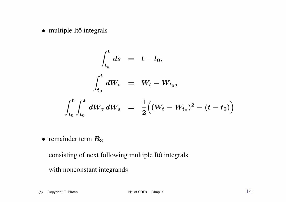
• multiple Ito integrals
∫ t
t0
ds = t − t0,
∫ t
t0
dWs = Wt − Wt0 ,∫ t
t0
∫ s
t0
dWz dWs =1
2
((Wt − Wt0)
2 − (t − t0))
• remainder term R3
consisting of next following multiple Ito integrals
with nonconstant integrands
c⃝ Copyright E. Platen NS of SDEs Chap. 1 14

Example
d=m = 1
for function f(t, x) ≡ x,
times ϱ= 0, τ = t
hierarchical set A = α ∈ Mm : ℓ(α) ≤ 3
drift a(t, x) = a(x)
diffusion coefficient b(t, x) = b(x)
dXt = a (Xt) dt + b(Xt) dWt
=⇒
Wagner-Platen expansion in the form:
c⃝ Copyright E. Platen NS of SDEs Chap. 1 15

Xt = X0 + a I(0) + b I(1) +
(a a′ +
1
2b2a′′
)I(0,0)
+
(a b′ +
1
2b2b′′
)I(0,1) + b a′I(1,0) + b b′I(1,1)
+
[a
(a a′′ + (a′)2 + b b′a′′ +
1
2b2a′′′
)+
1
2b2 (a a′′′ + 3 a′a′′
+((b′)2 + b b′′
)a′′ + 2 b b′a′′′)+ 1
4b4a(4)
]I(0,0,0)
+
[a
(a′b′ + a b′′ + b b′b′′ +
1
2b2b′′′
)+
1
2b2(a′′b′ + 2 a′b′′
+a b′′′ +((b′)2 + b b′′
)b′′ + 2 b b′b′′′ +
1
2b2b(4)
)]I(0,0,1)
c⃝ Copyright E. Platen NS of SDEs Chap. 1 16
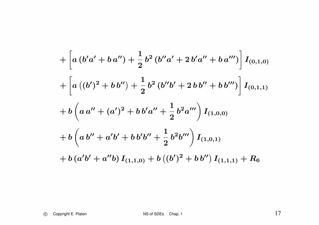
+
[a (b′a′ + b a′′) +
1
2b2 (b′′a′ + 2 b′a′′ + b a′′′)
]I(0,1,0)
+
[a((b′)2 + b b′′
)+
1
2b2 (b′′b′ + 2 b b′′ + b b′′′)
]I(0,1,1)
+ b
(a a′′ + (a′)2 + b b′a′′ +
1
2b2a′′′
)I(1,0,0)
+ b
(a b′′ + a′b′ + b b′b′′ +
1
2b2b′′′
)I(1,0,1)
+ b (a′b′ + a′′b) I(1,1,0) + b((b′)2 + b b′′
)I(1,1,1) + R6
c⃝ Copyright E. Platen NS of SDEs Chap. 1 17

Examples for Wagner Platen Expansions
• Vasicek interest rate model
drt = γ (r − rt) dt + β dWt
for t ∈ [0, T ], r0 ≥ 0
c⃝ Copyright E. Platen NS of SDEs Chap. 1 18
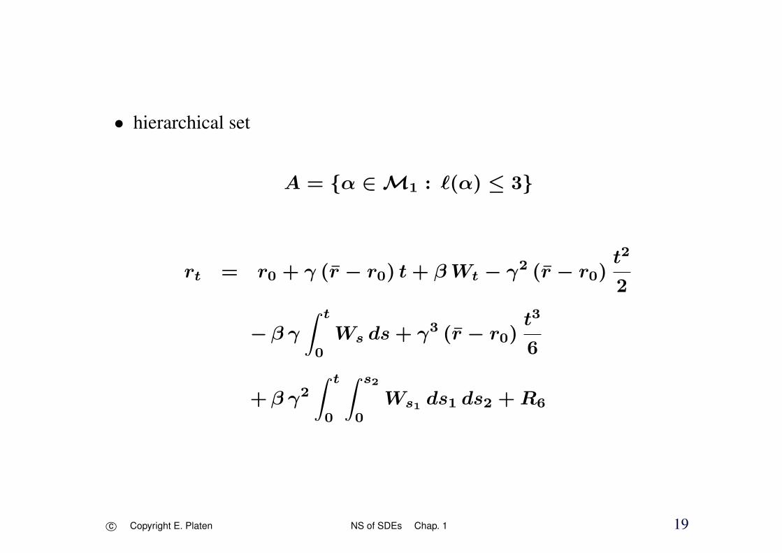
• hierarchical set
A = α ∈ M1 : ℓ(α) ≤ 3
rt = r0 + γ (r − r0) t + βWt − γ2 (r − r0)t2
2
−β γ
∫ t
0
Ws ds + γ3 (r − r0)t3
6
+β γ2
∫ t
0
∫ s2
0
Ws1 ds1 ds2 + R6
c⃝ Copyright E. Platen NS of SDEs Chap. 1 19

• Black-Scholes dynamics
dSt = St (a dt + σ dWt)
for t ∈ [0, T ], S0 ≥ 0
• Wagner-Platen expansion
hierarchical set
A = α ∈ M1 : ℓ(α) ≤ 3
c⃝ Copyright E. Platen NS of SDEs Chap. 1 20

is given by
St = S0
(1 + a t + σWt + a2 t2
2+ aσ (I(0,1) + I(1,0))
+σ2 1
2
((Wt)
2 − t)+ a3 t3
6
+ a2 σ (I(0,0,1) + I(0,1,0) + I(1,0,0))
+ aσ2 (I(0,1,1) + I(1,0,1) + I(1,1,0))
+σ3 1
6
((Wt)
3 − 3 tWt
))+R6
c⃝ Copyright E. Platen NS of SDEs Chap. 1 21

• relationship
tWt = I(0) I(1) = I(0,1) + I(1,0)
Wt
t2
2= I(1) I(0,0) = I(0,0,1) + I(0,1,0) + I(1,0,0)
t1
2
((Wt)
2 − t)
= I(0) I(1,1) = I(0,1,1) + I(1,0,1) + I(1,1,0)
c⃝ Copyright E. Platen NS of SDEs Chap. 1 22

• Wagner-Platen expansion
St = S0
(1 + a t + σWt + a2 t2
2+ aσ tWt
+σ2
2
((Wt)
2 − t)+ a3 t3
6+ a2σWt
t2
2
+ aσ2 t
2
((Wt)
2 − t)+ σ3 1
6
((Wt)
3 − 3 tWt
))+ R6
c⃝ Copyright E. Platen NS of SDEs Chap. 1 23

• squared Bessel process
dXt = ν dt + 2√
Xt dWt
for t ∈ [0, T ] with X0 > 0
hierarchical set
A = α ∈ M1 : ℓ(α) ≤ 2
c⃝ Copyright E. Platen NS of SDEs Chap. 1 24

• Wagner-Platen expansion
Xt = X0 + (ν − 1) t + 2√X0 Wt
+ν − 1√X0
∫ t
0
s dWs + (Wt)2 + R
c⃝ Copyright E. Platen NS of SDEs Chap. 1 25

2 Introduction to Scenario Simulation
Discrete Time Approximation
0 = τ0 < τ1 < · · · < τn < · · · < τN = T
one-dimensional SDE
dXt = a(t,Xt) dt + b(t,Xt) dWt
c⃝ Copyright E. Platen NS of SDEs Chap. 2 26

• Euler scheme
Euler-Maruyama scheme
Maruyama (1955)
Yn+1 = Yn+a(τn, Yn) (τn+1 − τn)+b(τn, Yn)(Wτn+1
− Wτn
)
Y0 = X0,
Yn = Yτn
∆n = τn+1 − τn
c⃝ Copyright E. Platen NS of SDEs Chap. 2 27

maximum step size
∆ = maxn∈0,1,...,N−1
∆n
• equidistant time discretization
τn = n∆
∆n ≡∆= TN
c⃝ Copyright E. Platen NS of SDEs Chap. 2 28

• Euler approximation recursively computed
• random increments
∆Wn = Wτn+1− Wτn
for n ∈ 0, 1, . . . , N−1
Wiener processW = Wt t ∈ [0, T ]
Gaussian distributed
meanE (∆Wn) = 0
varianceE((∆Wn)
2)= ∆n
c⃝ Copyright E. Platen NS of SDEs Chap. 2 29

Gaussian pseudo-random numbers generated
• abbreviationf = f(τn, Yn)
Euler scheme
Yn+1 = Yn + a∆n + b∆Wn,
discrete time approximations
c⃝ Copyright E. Platen NS of SDEs Chap. 2 30

Simulating Geometric Brownian Motion
• illustrate scenario simulation
standard market model as geometric Brownian motions
dXt = aXt dt + bXt dWt
for t ∈ [0, T ], X0 > 0
• drift coefficienta(t, x) = ax
• diffusion coefficientb(t, x) = b x
c⃝ Copyright E. Platen NS of SDEs Chap. 2 31

• appreciation rate a
• volatility b = 0
• explicit solution
Xt = X0 exp
((a −
1
2b2)t + bWt
)
• Wiener processW = Wt, t ∈ [0, T ]
c⃝ Copyright E. Platen NS of SDEs Chap. 2 32
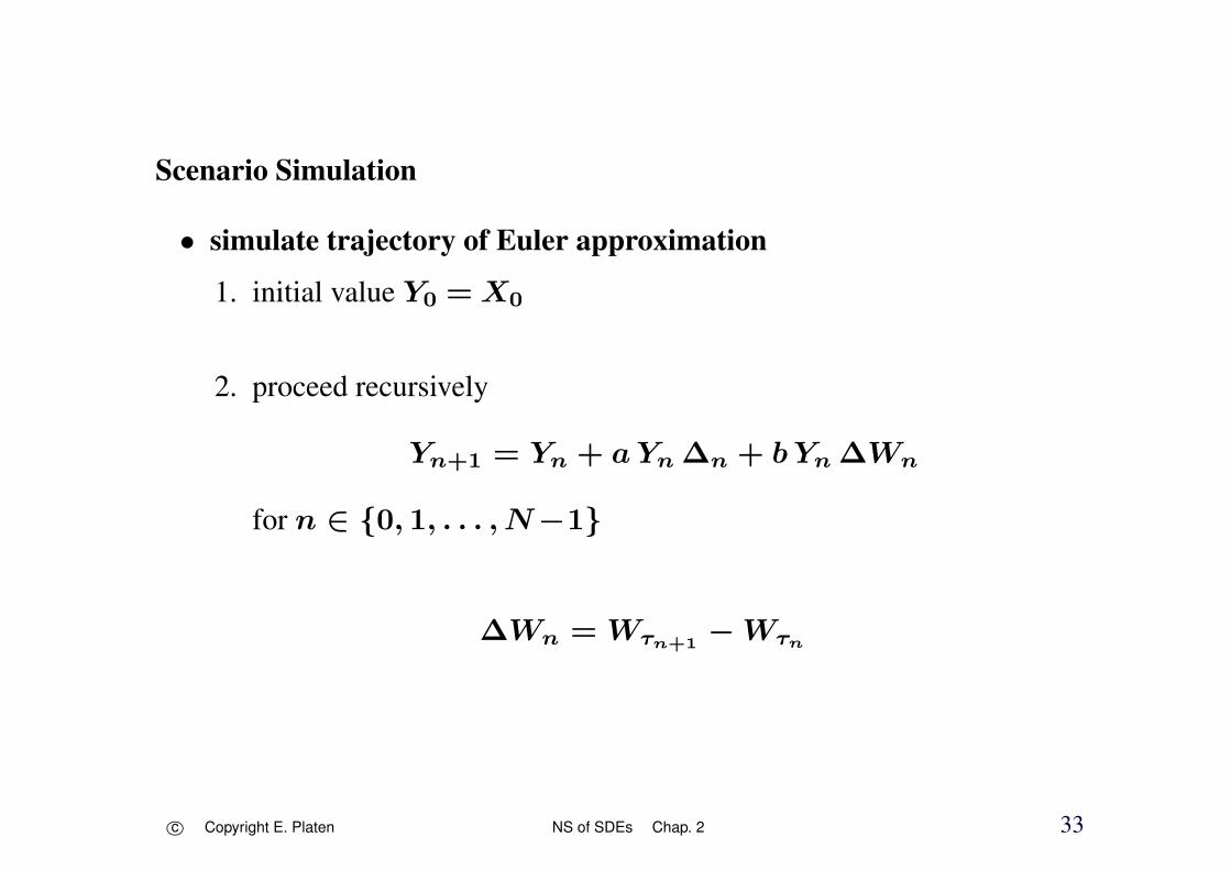
Scenario Simulation
• simulate trajectory of Euler approximation
1. initial value Y0 = X0
2. proceed recursively
Yn+1 = Yn + aYn ∆n + b Yn ∆Wn
for n ∈ 0, 1, . . . , N−1
∆Wn = Wτn+1− Wτn
c⃝ Copyright E. Platen NS of SDEs Chap. 2 33

• comparison with explicit solution at time τn
Xτn = X0 exp
((a −
1
2b2)τn + b
n∑i=1
∆Wi−1
)for n ∈ 0, 1, . . . , N−1Euler approximation
mathematically another new object
different
negative ?
alternative ways ?
c⃝ Copyright E. Platen NS of SDEs Chap. 2 34

0
2
4
6
8
10
0 0.2 0.4 0.6 0.8 1
Figure 2.1: Euler approximations for ∆ = 0.25 and ∆ = 0.0625 andexact solution for Black-Scholes SDE.
c⃝ Copyright E. Platen NS of SDEs Chap. 2 35

Strong Approximation
• not specified a criterion for classification
• scenario simulationapproximates paths
testing of calibration methods
statistical estimators
filtering
c⃝ Copyright E. Platen NS of SDEs Chap. 2 36

• Monte-Carlo simulation
approximates probabilities
functionals
simulates expectations
moments
prices of contingent claims
or risk measures as Value at Risk
c⃝ Copyright E. Platen NS of SDEs Chap. 2 37

Order of Strong Convergence
• absolute error criterion
ε(∆) = E(∣∣XT − Y ∆
T
∣∣)
A discrete time approximation Y ∆ converges strongly with order γ >
0 at time T if there exists a positive constant C, which does not dependon ∆, and a δ0 > 0 such that
ε(∆) = E(∣∣XT − Y ∆
T
∣∣) ≤ C ∆γ
for each ∆ ∈ (0, δ0).
c⃝ Copyright E. Platen NS of SDEs Chap. 2 38

Strong Taylor Schemes
• use Wagner-Platen expansions
appropriate truncation
• operators
L0 =∂
∂t+
d∑k=1
ak ∂
∂xk+
1
2
d∑k,ℓ=1
m∑j=1
bk,j bℓ,j∂
∂xk ∂xℓ
L0 =∂
∂t+
d∑k=1
ak ∂
∂xk
c⃝ Copyright E. Platen NS of SDEs Chap. 2 39

and
Lj = Lj =
d∑k=1
bk,j∂
∂xk
for j ∈ 1, 2, . . . ,m, where
ak = ak −1
2
m∑j=1
Lj bk,j
c⃝ Copyright E. Platen NS of SDEs Chap. 2 40

• multiple Ito integrals
I(j1,...,jℓ) =
∫ τn+1
τn
. . .
∫ s2
τn
dW j1s1
. . . dW jℓsℓ
• multiple Stratonovich integrals
J(j1,...,jℓ) =
∫ τn+1
τn
. . .
∫ s2
τn
dW j1s1
. . . dW jℓsℓ
for j1, . . . , jℓ ∈ 0, 1, . . . ,m, ℓ ∈ 1, 2, . . .and n ∈ 0, 1, . . .
W 0t = t
for all t ∈ [0, T ]
c⃝ Copyright E. Platen NS of SDEs Chap. 2 41

• Ito SDE
dXt = a(t,Xt) dt +m∑
j=1
bj(t,Xt) dWjt
• equivalent Stratonovich SDE
dXt = a(t,Xt) dt +m∑
j=1
bj(t,Xt) dW jt
c⃝ Copyright E. Platen NS of SDEs Chap. 2 42

Euler Scheme
simplest strong Taylor approximation
order of strong convergence γ = 0.5
• d =m= 1
Euler schemeYn+1 = Yn + a∆ + b∆W
∆ = τn+1 − τn
∆W = ∆Wn = Wτn+1− Wτn
N(0,∆) independent Gaussian distributed
c⃝ Copyright E. Platen NS of SDEs Chap. 2 43

• multi-dimensional Euler scheme
m = 1 and d ∈ 1, 2, . . .
kth component
Y kn+1 = Y k
n + ak ∆ + bk ∆W
for k ∈ 1, 2, . . . , d
a = (a1, . . ., ad)⊤ and b = (b1, . . ., bd)⊤
c⃝ Copyright E. Platen NS of SDEs Chap. 2 44

• general multi-dimensional Euler scheme
d, m ∈ 1, 2, . . .
Y kn+1 = Y k
n + ak ∆ +m∑
j=1
bk,j ∆W j
∆W j = W jτn+1
− W jτn
N(0,∆) independent Gaussian distributed
∆W j1 and ∆W j2 independent for j1 = j2
b = [bk,j]d,mk,j=1 d×m-matrix
truncated Wagner-Platen expansion
c⃝ Copyright E. Platen NS of SDEs Chap. 2 45

Theorem 2.1 Suppose that we have initial values X0 and Y0 = Y ∆0
such thatE(|X0|2
)< ∞
and
E(∣∣X0 − Y ∆
0
∣∣2) 12 ≤ K1 ∆
12 .
Furthermore, assume the Lipschitz condition
|a(t, x) − a(t, y)| + |b(t, x) − b(t, y)| ≤ K2 |x − y|,
the linear growth condition
|a(t, x)| + |b(t, x)| ≤ K3 (1 + |x| )
c⃝ Copyright E. Platen NS of SDEs Chap. 2 46

and
|a(s, x)−a(t, x)|+ |b(s, x)−b(t, x)| ≤ K4 (1 + |x| ) |s−t| 12
for all s, t ∈ [0, T ] and x, y ∈ ℜd, where the constants K1, . . ., K4 do
not depend on ∆. Then the Euler approximation Y ∆ converges with strongorder γ = 0.5, that is we have the estimate
E(∣∣XT − Y ∆
T
∣∣) ≤ K5 ∆12 ,
where the constant K5 does not depend on ∆.
c⃝ Copyright E. Platen NS of SDEs Chap. 2 47
A Simulation Example
• Black-Scholes SDE
dXt = µXt dt + σXt dWt
• exact solution
XT = X0 exp
(µ −
σ2
2
)T + σWT
c⃝ Copyright E. Platen NS of SDEs Chap. 2 48

absolute errorε(∆) = E(|XT − Y ∆
N |)
default parameters:
X0 = 1, µ = 0.06, σ = 0.2 and T = 1
5000 simulations
fitted line
ln(ε(∆)) = −3.86933 + 0.46739 ln(∆)
c⃝ Copyright E. Platen NS of SDEs Chap. 2 49

-4 -3 -2 -1 0
Log -dt
-6
-5.5
-5
-4.5
-4Log-Strong
Error
Figure 2.2: Log-log plot of the absolute error ε(∆) for an Euler Schemeagainst ln(∆).
c⃝ Copyright E. Platen NS of SDEs Chap. 2 50

Milstein Scheme
Milstein (1974)
• Milstein scheme
d = m = 1
Yn+1 = Yn + a∆ + b∆W +1
2b b′
(∆W )2 − ∆
order γ = 1.0 of strong convergence
c⃝ Copyright E. Platen NS of SDEs Chap. 2 51

• multi-dimensional Milstein scheme
m = 1 and d ∈ 1, 2, . . .
Y kn+1 = Y k
n +ak ∆+bk ∆W+
(d∑
ℓ=1
bℓ∂bk
∂xℓ
)1
2
(∆W )2 − ∆
c⃝ Copyright E. Platen NS of SDEs Chap. 2 52

• general multi-dimensional Milstein scheme
d, m ∈ 1, 2, . . .
kth component
Y kn+1 = Y k
n + ak ∆ +
m∑j=1
bk,j∆W j +
m∑j1,j2=1
Lj1bk,j2I(j1,j2)
Ito integrals I(j1,j2)
• alternatively
Y kn+1 = Y k
n + ak ∆ +m∑
j=1
bk,j∆W j +m∑
j1,j2=1
Lj1bk,j2J(j1,j2)
c⃝ Copyright E. Platen NS of SDEs Chap. 2 53

Stratonovich integrals J(j1,j2)
j1 = j2 j1, j2 ∈ 1, 2, . . . ,m
J(j1,j2) = I(j1,j2) =
∫ τn+1
τn
∫ s1
τn
dW j1s2
dW j2s1
cannot be simply expressed by ∆W j1 and ∆W j2
I(j1,j1) =1
2
(∆W j1)2 − ∆
and J(j1,j1) =
1
2
(∆W j1
)2
for j1 ∈ 1, 2, . . . ,m
c⃝ Copyright E. Platen NS of SDEs Chap. 2 54

Commutative Noise
• commutativity condition
Lj1bk,j2 = Lj2bk,j1
for all j1, j2 ∈ 1, 2, . . . ,m, k ∈ 1, 2, . . . , d and(t, x) ∈ [0, T ]×ℜd
• satisfied for Black-Scholes SDEs
additive noise
single Wiener process
c⃝ Copyright E. Platen NS of SDEs Chap. 2 55
• Milstein scheme under commutative noise
Y kn+1 = Y k
n +ak ∆+
m∑j=1
bk,j∆W j+1
2
m∑j1,j2=1
Lj1bk,j2∆W j1∆W j2
for k ∈ 1, 2, . . . , d
no double Wiener integrals
c⃝ Copyright E. Platen NS of SDEs Chap. 2 56

A Black-Scholes Example
• correlated Black-Scholes dynamics
d = m = 2
• first risky security
dX1t = X1
t
[r dt + θ1(θ1 dt + dW 1
t ) + θ2(θ2 dt + dW 2t )]
= X1t
[(r +
1
2
((θ1)2 + (θ2)2
))dt
+ θ1 dW 1t + θ2 dW 2
t
]
c⃝ Copyright E. Platen NS of SDEs Chap. 2 57

• second risky security
dX2t = X2
t
[r dt + (θ1 − σ1,1) (θ1 dt + dW 1
t )]
= X2t
[(r + (θ1 − σ1,1)
(1
2θ1 +
1
2σ1,1
))dt
+(θ1 − σ1,1) dW 1t
]
c⃝ Copyright E. Platen NS of SDEs Chap. 2 58
=⇒
L1 b1,2 =2∑
k=1
bk,1∂
∂xkb1,2 = θ1 X1
t θ2
=2∑
k=1
bk,2∂
∂xkb1,1 = L2 b1,1
and
L1 b2,2 =2∑
k=1
bk,1∂
∂xkb2,2 = 0 =
2∑k=1
bk,2∂
∂xkb2,1 = L2 b2,1
=⇒ commutativity condition satisfied
=⇒ Milstein scheme :
c⃝ Copyright E. Platen NS of SDEs Chap. 2 59

Y 1n+1 = Y 1
n + Y 1n
(r +
1
2
((θ1)2 + (θ2)2
)∆ + θ1 ∆W 1 + θ2 ∆W 2
+1
2(θ1)2(∆W 1)2 +
1
2(θ2)2(∆W 2)2 + θ1 θ2 ∆W 1 ∆W 2
)
Y 2n+1 = Y 2
n + Y 2n
((r +
1
2(θ1 − σ1,1) (θ1 + σ1,1)
)∆
+(θ1 − σ1,1)∆W 1 +1
2(θ1 − σ1,1)2 (∆W 1)2
)
( may produce negative trajectories )
c⃝ Copyright E. Platen NS of SDEs Chap. 2 60

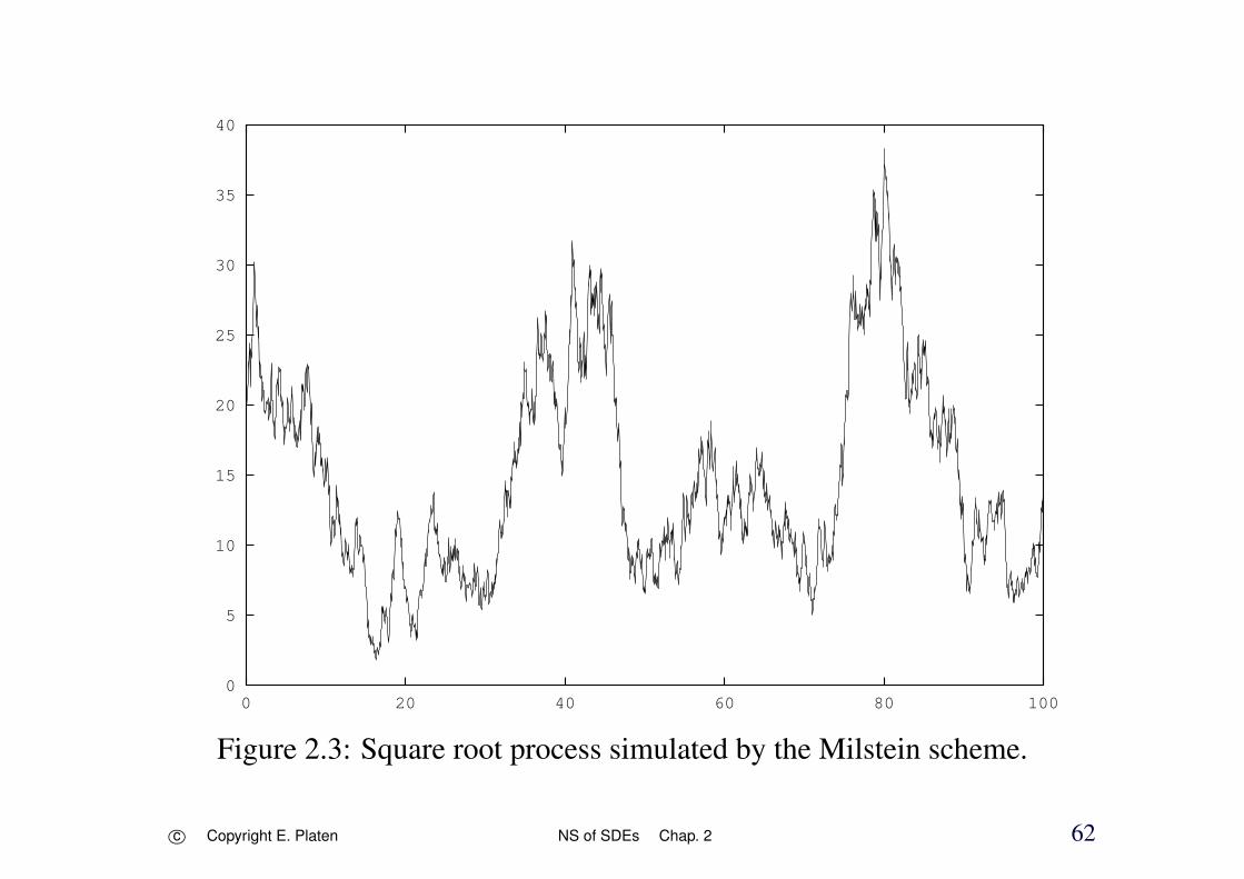
A Square Root Process Example
• square root process of dimension ν
dXt =ν
4η
(1
η− Xt
)dt +
√Xt dW
1t
X0 = 1η
for ν > 2
• Milstein
Yn+1 = Yn+ν
4η
(1
η− Yn
)∆+
√Yn ∆W +
1
4
(∆W 2 − ∆
)
c⃝ Copyright E. Platen NS of SDEs Chap. 2 61
0
5
10
15
20
25
30
35
40
0 20 40 60 80 100
Figure 2.3: Square root process simulated by the Milstein scheme.
c⃝ Copyright E. Platen NS of SDEs Chap. 2 62

Convergence Theorem
E(|X0|2
)< ∞
E(∣∣X0 − Y ∆
0
∣∣2) 12 ≤ K1 ∆
12
c⃝ Copyright E. Platen NS of SDEs Chap. 2 63

|a(t, x) − a(t, y)| ≤ K2 |x − y|∣∣bj1(t, x) − bj1(t, y)∣∣ ≤ K2 |x − y|∣∣∣Lj1bj2(t, x) − Lj1bj2(t, y)∣∣∣ ≤ K2 |x − y|
|a(t, x)| +∣∣∣Lja(t, x)
∣∣∣ ≤ K3 (1 + |x|)∣∣bj1(t, x)∣∣+ ∣∣∣Ljbj2(t, x)∣∣∣ ≤ K3 (1 + |x|)∣∣∣LjLj1bj2(t, x)∣∣∣ ≤ K3 (1 + |x|)
c⃝ Copyright E. Platen NS of SDEs Chap. 2 64

and
|a(s, x) − a(t, x)| ≤ K4 (1 + |x| ) |s − t| 12∣∣bj1(s, x) − bj1(t, x)
∣∣ ≤ K4 (1 + |x| ) |s − t| 12∣∣∣Lj1bj2(s, x) − Lj1bj2(t, x)
∣∣∣ ≤ K4 (1 + |x| ) |s − t| 12
for all s, t∈ [0, T ], x, y∈ℜd, j ∈ 0, . . ., m and j1, j2 ∈ 1, 2, . . . ,m.Then the Milstein scheme converges with strong order γ = 1.0
E(∣∣XT − Y ∆
T
∣∣) ≤ K5 ∆.
Kloeden & Pl. (1992b).
c⃝ Copyright E. Platen NS of SDEs Chap. 2 65

A Simulation Study
-4 -3 -2 -1 0
Log -dt
-9
-8
-7
-6
-5Log-Strong
Error
Figure 2.4: Log-log plot of the absolute error against log-step size for aMilstein scheme.
c⃝ Copyright E. Platen NS of SDEs Chap. 2 66

• linear regression
ln(ε(∆)) = −4.91021 + 0.95 ln(∆)
c⃝ Copyright E. Platen NS of SDEs Chap. 2 67

Order 1.5 Strong Taylor Scheme
• simulation tasks that require more accurate schemes
extreme log-returns
• including further multiple stochastic integrals
• order 1.5 strong Taylor scheme
d = m = 1
c⃝ Copyright E. Platen NS of SDEs Chap. 2 68

Yn+1 = Yn + a∆ + b∆W +1
2b b′
(∆W )2 − ∆
+ a′ b∆Z +
1
2
(a a′ +
1
2b2 a′′
)∆2
+
(a b′ +
1
2b2 b′′
)∆W ∆ − ∆Z
+1
2b(b b′′ + (b′)2
) 1
3(∆W )2 − ∆
∆W
c⃝ Copyright E. Platen NS of SDEs Chap. 2 69

• double integral
∆Z = I(1,0) =
∫ τn+1
τn
∫ s2
τn
dWs1 ds2
Gaussian
E(∆Z) = 0
E((∆Z)2) =1
3∆3
E(∆Z ∆W ) =1
2∆2
c⃝ Copyright E. Platen NS of SDEs Chap. 2 70

• two independent N(0, 1)
U1 and U2
=⇒
∆W = U1
√∆, ∆Z =
1
2∆
32
(U1 +
1√3U2
)
• triple Wiener integral
I(1,1,1) =1
2
1
3(∆W 1)2 − ∆
∆W 1
scaled monic Hermite polynomial
c⃝ Copyright E. Platen NS of SDEs Chap. 2 71

• multi-dimensional order 1.5 strong Taylor scheme
d ∈ 1, 2, . . . and m = 1
Y kn+1 = Y k
n + ak ∆ + bk ∆W
+1
2L1 bk (∆W )2 − ∆ + L1 ak ∆Z
+L0 bk ∆W ∆ − ∆Z +1
2L0 ak ∆2
+1
2L1 L1 bk
1
3(∆W )2 − ∆
∆W
c⃝ Copyright E. Platen NS of SDEs Chap. 2 72

• general multi-dimensional order 1.5 strong Taylor scheme
d,m ∈ 1, 2, . . .
Y kn+1 = Y k
n + ak ∆ +1
2L0 ak ∆2
+m∑
j=1
(bk,j∆W j + L0 bk,j I(0,j) + Lj ak I(j,0))
+
m∑j1,j2=1
Lj1 bk,j2 I(j1,j2) +
m∑j1,j2,j3=1
Lj1 Lj2 bk,j3 I(j1,j2,j3)
in case of additive noise simplifies considerably
strong order γ = 1.5
c⃝ Copyright E. Platen NS of SDEs Chap. 2 73

Approximate Multiple Stochastic Integrals
Let ξj , ζj,1, . . . , ζj,p, ηj,1, . . . , ηj,p, µj,p and ϕj,p
be independent N(0, 1)
for j, j1, j2, j3 ∈ 1, 2, . . . ,m and some p ∈ 1, 2, . . .
set
I(j) = ∆W j =√∆ ξj, I(j,0) =
1
2∆(√
∆ ξj + aj,0
)
with
aj,0 = −√2∆
π
p∑r=1
1
rζj,r − 2
√∆ ϱp µj,p
c⃝ Copyright E. Platen NS of SDEs Chap. 2 74
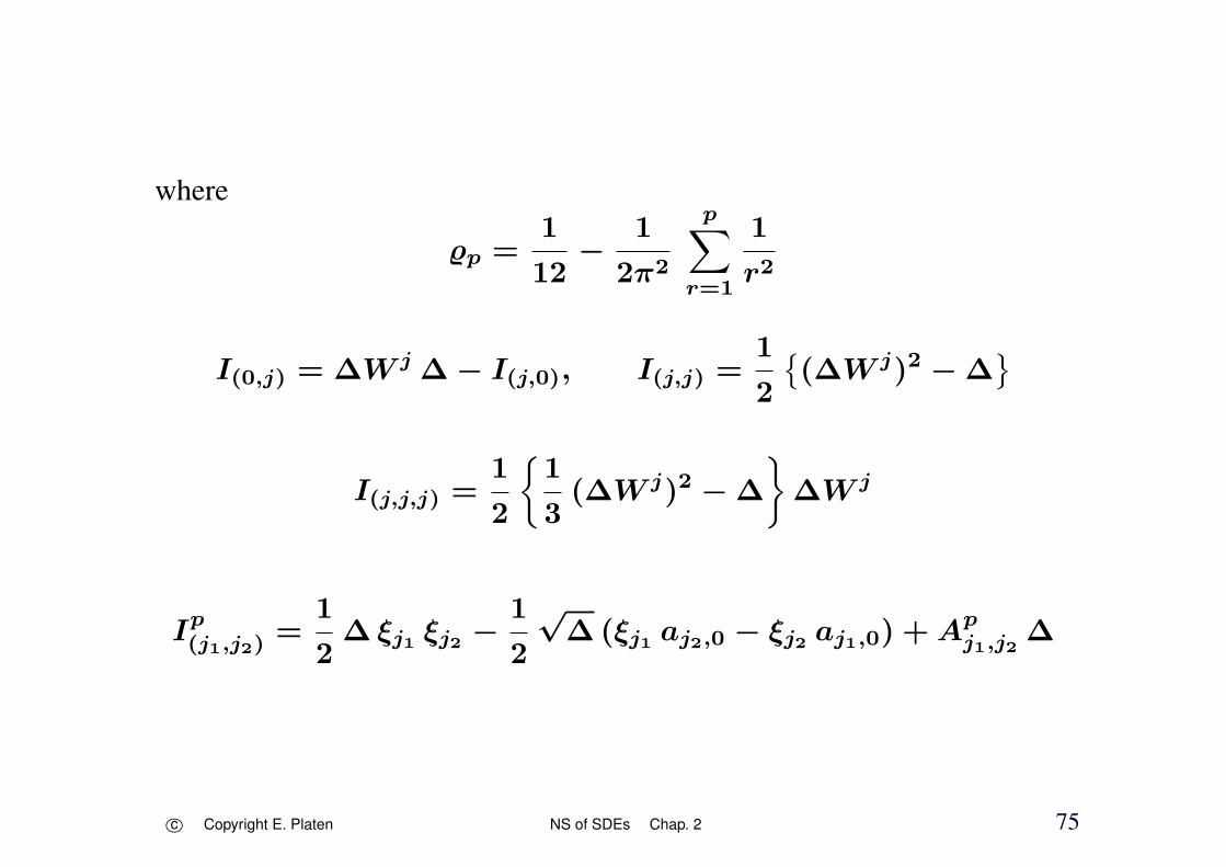
where
ϱp =1
12−
1
2π2
p∑r=1
1
r2
I(0,j) = ∆W j ∆ − I(j,0), I(j,j) =1
2
(∆W j)2 − ∆
I(j,j,j) =1
2
1
3(∆W j)2 − ∆
∆W j
Ip(j1,j2)
=1
2∆ ξj1 ξj2 −
1
2
√∆(ξj1 aj2,0 − ξj2 aj1,0) + Ap
j1,j2∆
c⃝ Copyright E. Platen NS of SDEs Chap. 2 75

Order 2.0 Strong Taylor Scheme
• use Stratonovich-Taylor expansion
d =m= 1
Yn+1 = Yn + a∆ + b∆W +1
2!b b′(∆W )2 + b a′ ∆Z
+1
2a a′ ∆2 + a b′∆W ∆ − ∆Z
+1
3!b (b b′)
′(∆W )3 +
1
4!b(b (b b′)
′)′
(∆W )4
+ a (b b′)′J(0,1,1) + b (a b′)
′J(1,0,1) + b (b a′)
′J(1,1,0)
c⃝ Copyright E. Platen NS of SDEs Chap. 2 76
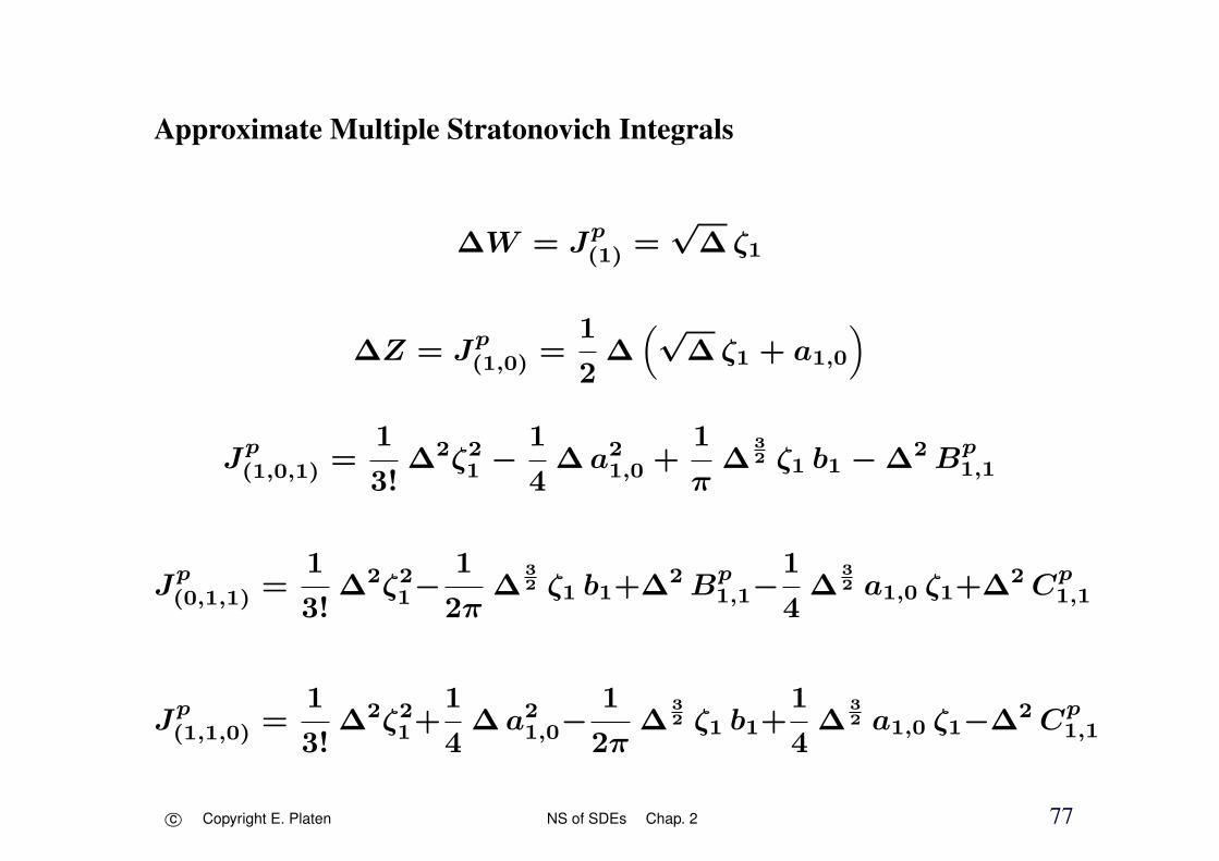
Approximate Multiple Stratonovich Integrals
∆W = Jp(1) =
√∆ ζ1
∆Z = Jp(1,0) =
1
2∆(√
∆ ζ1 + a1,0
)
Jp(1,0,1) =
1
3!∆2ζ2
1 −1
4∆ a2
1,0 +1
π∆
32 ζ1 b1 − ∆2 Bp
1,1
Jp(0,1,1) =
1
3!∆2ζ2
1−1
2π∆
32 ζ1 b1+∆2 Bp
1,1−1
4∆
32 a1,0 ζ1+∆2 Cp
1,1
Jp(1,1,0) =
1
3!∆2ζ2
1+1
4∆ a2
1,0−1
2π∆
32 ζ1 b1+
1
4∆
32 a1,0 ζ1−∆2 Cp
1,1
c⃝ Copyright E. Platen NS of SDEs Chap. 2 77

with
a1,0 = −1
π
√2∆
p∑r=1
1
rξ1,r − 2
√∆ϱp µ1,p
ϱp =1
12−
1
2π2
p∑r=1
1
r2
b1 =
√∆
2
p∑r=1
1
r2η1,r +
√∆αp ϕ1,p
αp =π2
180−
1
2π2
p∑r=1
1
r4
Bp1,1 =
1
4π2
p∑r=1
1
r2
(ξ21,r + η2
1,r
)
c⃝ Copyright E. Platen NS of SDEs Chap. 2 78

and
Cp1,1 = −
1
2π2
p∑r,l=1r =l
r
r2 − l2
(1
lξ1,r ξ1,ℓ −
l
rη1,r η1,ℓ
)
ζ1, ξ1,r η1,r, µ1,p and ϕ1,p ∼ N(0, 1) i.i.d.
c⃝ Copyright E. Platen NS of SDEs Chap. 2 79

Multi-dimensional Order 2.0 Strong Taylor Scheme
m= 1
Y kn+1 = Y k
n + ak ∆ + bk ∆W +1
2!L1 bk (∆W )2 + L1 ak ∆Z
+1
2L0ak ∆2 + L0bk ∆W ∆ − ∆Z
+1
3!L1L1bk (∆W )3 +
1
4!L1L1L1bk (∆W )4
+L0L1bk J(0,1,1) + L1L0bk J(1,0,1) + L1L1ak J(1,1,0)
c⃝ Copyright E. Platen NS of SDEs Chap. 2 80

• general multi-dimensional order 2.0 strong Taylor scheme
Y kn+1 = Y k
n + ak ∆ +1
2L0ak ∆2
+m∑
j=1
(bk,j ∆W j + L0bk,jJ(0,j) + Ljak J(j,0)
)
+m∑
j1,j2=1
(Lj1bk,j2J(j1,j2) + L0Lj1bk,j2J(0,j1,j2)
+Lj1L0bk,j2J(j1,0,j2) + Lj1Lj2ak J(j1,j2,0)
)
+m∑
j1,j2,j3=1
Lj1Lj2bk,j3J(j1,j2,j3)
+
m∑j1,j2,j3,j4=1
Lj1Lj2Lj3bk,j4J(j1,j2,j3,j4)
c⃝ Copyright E. Platen NS of SDEs Chap. 2 81
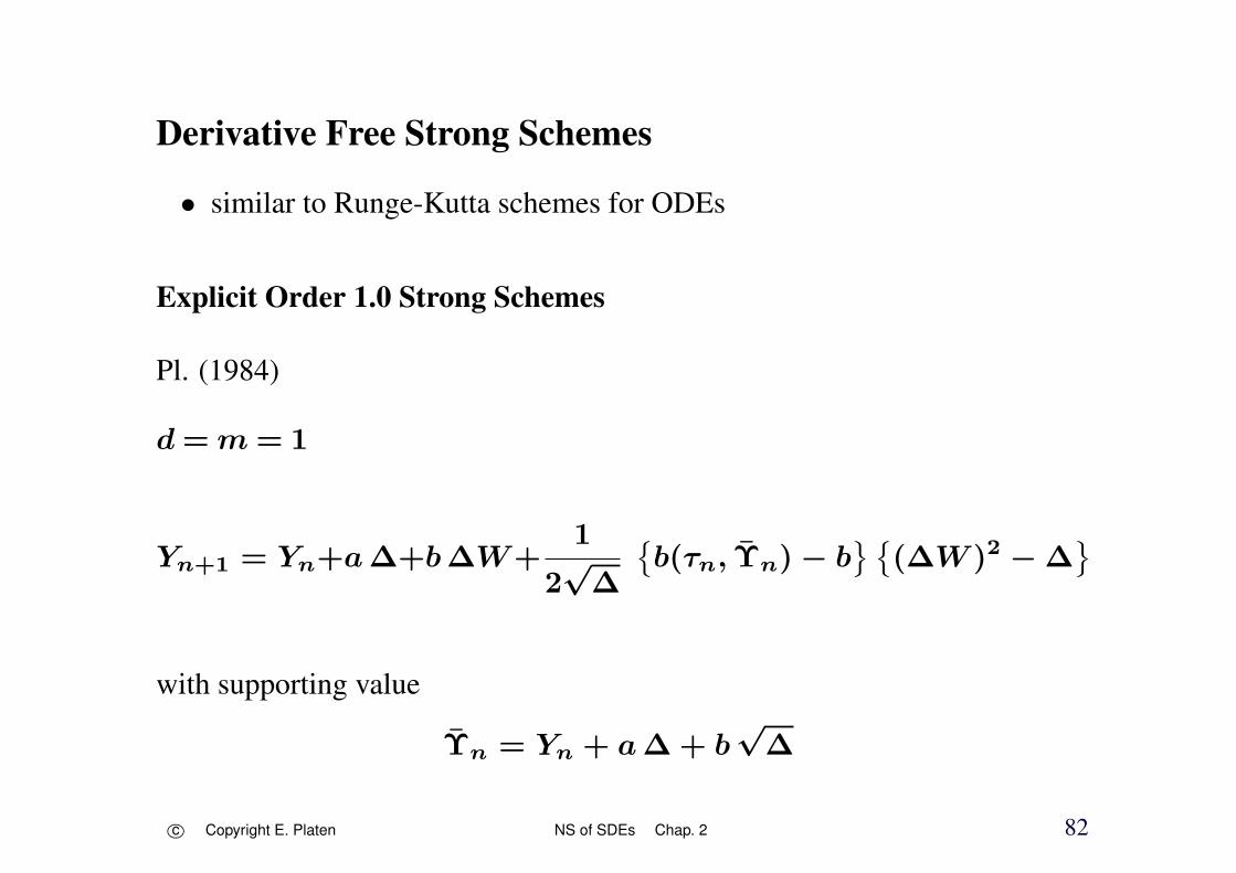
Derivative Free Strong Schemes
• similar to Runge-Kutta schemes for ODEs
Explicit Order 1.0 Strong Schemes
Pl. (1984)
d=m = 1
Yn+1 = Yn+a∆+b∆W+1
2√∆
b(τn, Υn) − b
(∆W )2 − ∆
with supporting value
Υn = Yn + a∆ + b√∆
c⃝ Copyright E. Platen NS of SDEs Chap. 2 82

• multi-dimensional Platen scheme
m = 1
Y kn+1 = Y k
n + ak ∆ + bk ∆W
+1
2√∆
(bk(τn, Υn) − bk
) ((∆W )2 − ∆
)
with the vector supporting value
Υn = Yn + a∆ + b√∆
c⃝ Copyright E. Platen NS of SDEs Chap. 2 83
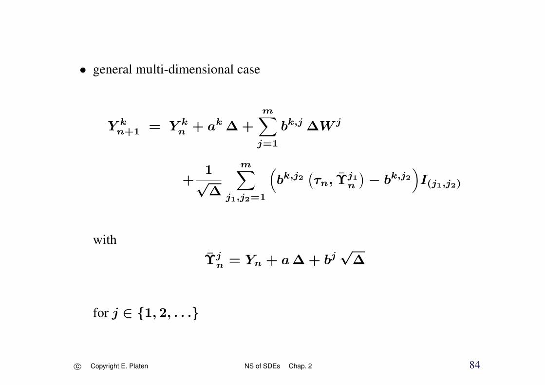
• general multi-dimensional case
Y kn+1 = Y k
n + ak ∆ +m∑
j=1
bk,j ∆W j
+1
√∆
m∑j1,j2=1
(bk,j2
(τn, Υ
j1n
)− bk,j2
)I(j1,j2)
withΥj
n = Yn + a∆ + bj√∆
for j ∈ 1, 2, . . .
c⃝ Copyright E. Platen NS of SDEs Chap. 2 84

• commutative noise
Y kn+1 = Y k
n + ak ∆ +1
2
m∑j=1
(bk,j
(τn, Υn
)+ bk,j
)∆W j
with
Υn = Yn + a∆ +m∑
j=1
bj ∆W j
strong order γ = 1.0
c⃝ Copyright E. Platen NS of SDEs Chap. 2 85

ln(ε(∆)) = −4.71638 + 0.946112 ln(∆)
-4 -3 -2 -1 0
Log -dt
-9
-8
-7
-6
-5Log-Strong
Error
Figure 2.5: Log-log plot of the absolute error for a Platen scheme.
c⃝ Copyright E. Platen NS of SDEs Chap. 2 86

• two stage Runge-Kutta method γ = 1.0
m = d = 1
Burrage (1998)
Yn+1 = Yn +(a(Yn) + 3 a(Yn)
) ∆
4
+1
4
(b(Yn) + 3 b(Yn)
)∆W
with
Yn = Yn +2
3(a(Yn)∆ + b(Yn)∆W )
c⃝ Copyright E. Platen NS of SDEs Chap. 2 87

Explicit Order 1.5 Strong Schemes
Pl. (1984)
d = m = 1
withΥ± = Yn + a∆ ± b
√∆
and
Φ± = Υ+ ± b(Υ+)√∆
c⃝ Copyright E. Platen NS of SDEs Chap. 2 88

Yn+1 = Yn + b∆W +1
2√∆
(a(Υ+) − a(Υ−)
)∆Z
+1
4
(a(Υ+) + 2a + a(Υ−)
)∆
+1
4√∆
(b(Υ+) − b(Υ−)
) ((∆W )2 − ∆
)+
1
2∆
(b(Υ+) − 2b + b(Υ−)
) (∆W∆ − ∆Z
)+
1
4∆
(b(Φ+) − b(Φ−) − b(Υ+) + b(Υ−)
)×(1
3(∆W )2 − ∆
)∆W
c⃝ Copyright E. Platen NS of SDEs Chap. 2 89
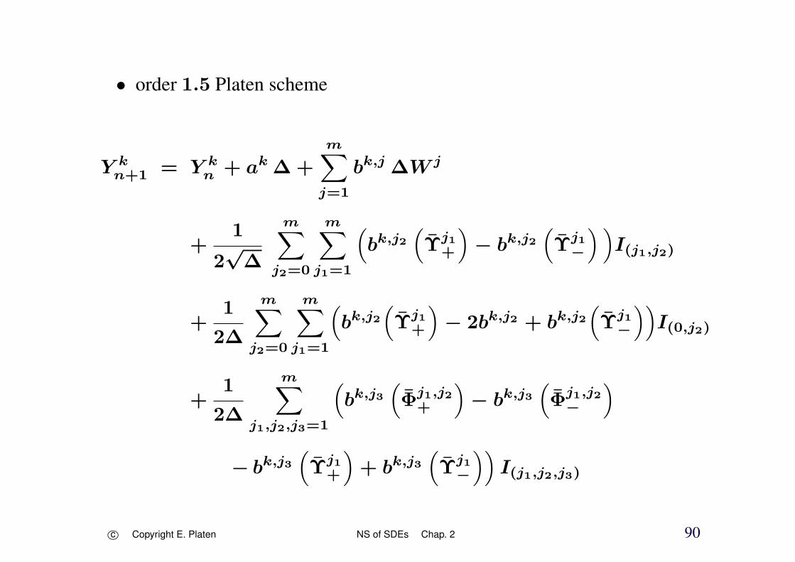
• order 1.5 Platen scheme
Y kn+1 = Y k
n + ak ∆ +
m∑j=1
bk,j ∆W j
+1
2√∆
m∑j2=0
m∑j1=1
(bk,j2
(Υj1
+
)− bk,j2
(Υj1
−
) )I(j1,j2)
+1
2∆
m∑j2=0
m∑j1=1
(bk,j2
(Υj1
+
)− 2bk,j2 + bk,j2
(Υj1
−
))I(0,j2)
+1
2∆
m∑j1,j2,j3=1
(bk,j3
(Φj1,j2
+
)− bk,j3
(Φj1,j2
−
)− bk,j3
(Υj1
+
)+ bk,j3
(Υj1
−
))I(j1,j2,j3)
c⃝ Copyright E. Platen NS of SDEs Chap. 2 90
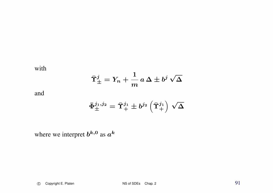
with
Υj± = Yn +
1
ma∆ ± bj
√∆
and
Φj1,j2± = Υj1
+ ± bj2(Υj1
+
) √∆
where we interpret bk,0 as ak
c⃝ Copyright E. Platen NS of SDEs Chap. 2 91
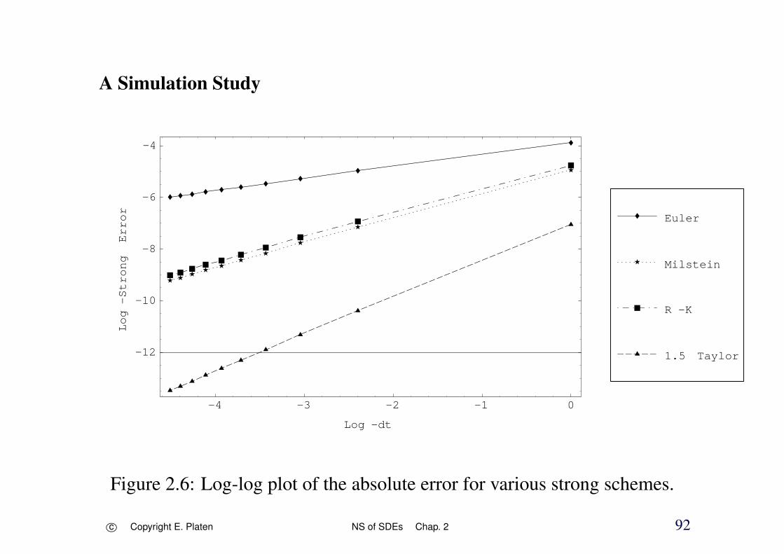
A Simulation Study
-4 -3 -2 -1 0
Log -dt
-12
-10
-8
-6
-4
Log-Strong
Error
1.5 Taylor
R -K
Milstein
Euler
Figure 2.6: Log-log plot of the absolute error for various strong schemes.
c⃝ Copyright E. Platen NS of SDEs Chap. 2 92

Method CPU Time
Euler 3.5 Seconds
Milstein 4.1 Seconds
1.0 Strong Platen 4.1 Seconds
1.5 Strong Taylor 4.4 Seconds
Table 1: Computational times for various strong methods.
500000 time steps
c⃝ Copyright E. Platen NS of SDEs Chap. 2 93

Numerical Stability
• ability of a scheme to control the propagationof initial and roundoff errors
• numerical stability has higher priority thana potentially high strong order
c⃝ Copyright E. Platen NS of SDEs Chap. 2 94

Deterministic A-Stability
• one-step method
Yn+1 = Yn + Ψ(τn, Yn, Yn+1,∆)∆
ordinary differential equation
dx
dt= a(t, x)
a(t, x) satisfies Lipschitz condition
c⃝ Copyright E. Platen NS of SDEs Chap. 2 95

• numerically stable
if there exist positive constants ∆0 and M such that
|Yn − Yn| ≤ M |Y0 − Y0|
n ∈ 0, 1, . . . , N, ∆ < ∆0
and any two solutions Y , Ycorresponding to the initial values Y0 Y0, respectively
• asymptotically numerically stable
if there exist ∆0 and M such that
limn→∞
|Yn − Yn| ≤ M |Y0 − Y0|
for any two Y , Y
c⃝ Copyright E. Platen NS of SDEs Chap. 2 96

• test equation
dxt
dt= λxt
with λ ∈ ℜ
c⃝ Copyright E. Platen NS of SDEs Chap. 2 97

numerical scheme in recursive form
Yn+1 = G(λ∆)Yn
• A-stability region:
those λ∆ ∈ ℜ for which
|G(λ∆)| < 1
c⃝ Copyright E. Platen NS of SDEs Chap. 2 98

• explicit Euler scheme
Yn+1 = Yn + a(tn, Yn)∆
Yn+1 = (1 + λ∆)Yn
A-stability region
open unit interval centered at −1 and ending at 0 since
|G(λ∆)| = |1 + λ∆|
c⃝ Copyright E. Platen NS of SDEs Chap. 2 99

-2 -1 0
-1
-0.5
0.5
1
Figure 2.7: Region of A-stability for the deterministic Euler scheme.
c⃝ Copyright E. Platen NS of SDEs Chap. 2 100

• implicit Euler scheme
Yn+1 = Yn + a(tn+1, Yn+1)∆
Yn+1 = Yn + λ∆Yn+1
(1 − λ∆)Yn+1 = Yn
G(λ∆) =1
1 − λ∆
|G(λ∆)| =1
|1 − λ∆|
exterior of an interval with center at 1 beginning at 0
• scheme is called A-stable if it covers at least the left half axis
c⃝ Copyright E. Platen NS of SDEs Chap. 2 101

Stochastic A-Stability
• test equation
dXt = λXt dt + dWt
λ ∈ ℜ
c⃝ Copyright E. Platen NS of SDEs Chap. 2 102

• discrete time approximation
Yn+1 = GA(λ∆)Yn + Zn,
Zn does not depend on Y0, Y1, . . . , Yn, Yn+1
c⃝ Copyright E. Platen NS of SDEs Chap. 2 103

• A-stability region
real numbers λ∆ for which
|GA(λ∆)| < 1
If A-stability region covers left half of the real axis
=⇒ then A-stable
c⃝ Copyright E. Platen NS of SDEs Chap. 2 104

Drift Implicit Euler Scheme
• drift implicit Euler scheme
strong order γ = 0.5
d = m = 1
Yn+1 = Yn + a (τn+1, Yn+1) ∆ + b∆W
c⃝ Copyright E. Platen NS of SDEs Chap. 2 105

• family of drift implicit Euler schemes
Yn+1 = Yn + αa (τn+1, Yn+1) + (1 − α) a ∆ + b∆W
degree of implicitness α ∈ [0, 1]
for α = 0 explicit Euler scheme
for α = 1 drift implicit Euler scheme
c⃝ Copyright E. Platen NS of SDEs Chap. 2 106

• general multi-dimensional
family of drift implicit Euler schemes
Y kn+1 = Y k
n +(αka
k (τn+1, Yn+1) + (1 − αk) ak)∆
+m∑
j=1
bk,j ∆W j
αk ∈ [0, 1], k ∈ 1, 2, . . . , d
c⃝ Copyright E. Platen NS of SDEs Chap. 2 107

• for test equation
Yn+1 = Yn +(αλYn+1 + (1 − α)λYn
)∆ + ∆Wn
Yn+1 = GA(λ∆)Yn + ∆Wn (1 − αλ∆)−1
transfer function
GA(λ∆) = (1 − αλ∆)−1 (1 + (1 − α)λ∆)
c⃝ Copyright E. Platen NS of SDEs Chap. 2 108

Yn corresponding discrete time approximation that starts at initial value Y0
Yn+1 − Yn+1 = GA(λ∆) (Yn − Yn)
= (GA(λ∆))n (Y0 − Y0)
as long as|GA(λ∆)| < 1
the initial error (Y0 − Y0) is decreased
=⇒ λ∆ ∈(−
2
1 − 2α, 0
)for α ≥ 1
2A-stable
c⃝ Copyright E. Platen NS of SDEs Chap. 2 109
Drift Implicit Milstein Scheme
d = m = 1
• Ito version
Yn+1 = Yn+a (τn+1, Yn+1) ∆+b∆W+1
2b b′((∆W )2−∆
)
c⃝ Copyright E. Platen NS of SDEs Chap. 2 110

• Stratonovich version
Yn+1 = Yn + a (τn+1, Yn+1) ∆ + b∆W +1
2b b′(∆W )2
adjusted Stratonovich drift a = a − 12b b′
both schemes are different
c⃝ Copyright E. Platen NS of SDEs Chap. 2 111

• multi-dimensional case with d = m ∈ 1, 2, . . . and commutativenoise
Y kn+1 = Y k
n +αk ak (τn+1, Yn+1) + (1 − αk) a
k∆
+
m∑j=1
bk,j ∆W j
+1
2
m∑j1,j2=1
Lj1bk,j2∆W j1∆W j2 − 1j1=j2∆
and
Y kn+1 = Y k
n +αk ak (τn+1, Yn+1) + (1 − αk) a
k∆
+m∑
j=1
bk,j ∆W j +1
2
m∑j1,j2=1
Lj1bk,j2∆W j1∆W j2
c⃝ Copyright E. Platen NS of SDEs Chap. 2 112

• general drift implicit Milstein scheme
Ito version
Y kn+1 = Y k
n +(αk ak (τn+1, Yn+1) + (1 − αk) a
k)∆
+
m∑j=1
bk,j ∆W j +
m∑j1,j2=1
Lj1bk,j2I(j1,j2)
c⃝ Copyright E. Platen NS of SDEs Chap. 2 113

Stratonovich version
Y kn+1 = Y k
n +(αk ak (τn+1, Yn+1) + (1 − αk) a
k)∆
+m∑
j=1
bk,j ∆W j +m∑
j1,j2=1
Lj1bk,j2J(j1,j2)
αk ∈ [0, 1] for k ∈ 1,. . ., d
multiple stochastic integrals I(j1,j2) and J(j1,j2)
approximated
c⃝ Copyright E. Platen NS of SDEs Chap. 2 114

Drift Implicit Order 1.0 Strong Runge-Kutta Scheme
d=m = 1
Yn+1 = Yn + a (τn+1, Yn+1) ∆ + b∆W
+1
2√∆
(b(τn, Υn
)− b
) ((∆W )2 − ∆
)
with supporting value
Υ = Yn + a∆ + b√∆
c⃝ Copyright E. Platen NS of SDEs Chap. 2 115

• family of drift implicit order 1.0 strong Runge-Kutta schemes
Y kn+1 = Y k
n +(αk a (τn+1, Yn+1) + (1 − αk) a
k)∆
+m∑
j=1
bk,j ∆W j
+1
√∆
m∑j1,j2=1
(bk,j2
(τn, Υ
j1n
)− bk,j2
)I(j1,j2)
withΥj
n = Yn + a∆ + bj√∆
for j ∈ 1, 2, . . . ,mαk ∈ [0, 1] for k ∈ 1, 2, . . . , d
c⃝ Copyright E. Platen NS of SDEs Chap. 2 116

• for commutative noise
Y kn+1 = Y k
n +(αk ak (τn+1, Yn+1) + (1 − αk) ak
)∆
+1
2
m∑j=1
(bk,j
(τn, Ψn
)+ bk,j
)∆W j
with
Ψn = Yn + a∆ +
m∑j=1
bj ∆W j
αk ∈ [0, 1] for k ∈ 1, 2, . . . , d
c⃝ Copyright E. Platen NS of SDEs Chap. 2 117

Alternative Implicit Methods
• implicit methods are important
• overcome a range of numerical instabilities
• the above strong schemes do not provide implicit diffusion terms
=⇒ important limitation
• drift implicit methods are well adapted for small noise and additive noisefor relatively large multiplicative noise
implicit diffusion terms seem unavoidable
c⃝ Copyright E. Platen NS of SDEs Chap. 2 118

• illustration with multiplicative noise
dXt = σXt dWt
• explicit strong methods have large errors for not too small time step sizes
• very small time step size may require unrealistic computational time
• cannot apply drift implicit schemes
c⃝ Copyright E. Platen NS of SDEs Chap. 2 119
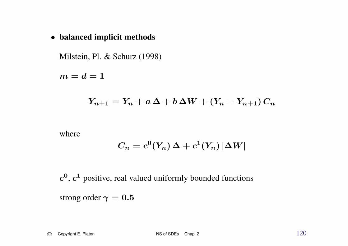
• balanced implicit methods
Milstein, Pl. & Schurz (1998)
m = d = 1
Yn+1 = Yn + a∆ + b∆W + (Yn − Yn+1)Cn
whereCn = c0(Yn)∆ + c1(Yn) |∆W |
c0, c1 positive, real valued uniformly bounded functions
strong order γ = 0.5
c⃝ Copyright E. Platen NS of SDEs Chap. 2 120

• low order strong convergence
price to pay for numerical stability
• family of specific methods providing a balance between approximatingdiffusion terms
c⃝ Copyright E. Platen NS of SDEs Chap. 2 121

Simulation Study for the Balanced Method
• Euler schemeYn+1 = Yn + σ Yn ∆W
• no simple stochastic counterpart of deterministic implicit Euler methodsince
Yn+1 = Yn + σ Yn+1 ∆W
Yn+1 =Yn
1 − σ∆W
fails becauseE|(1 − σ∆W )−1| = +∞
c⃝ Copyright E. Platen NS of SDEs Chap. 2 122

• partially implicit scheme
Yn+1 = Yn +
(σ∆W +
σ2
2(∆W )2
)Yn −
σ2
2Yn+1 ∆
• balanced implicit method
Yn+1 = Yn + σ Yn ∆W + σ (Yn − Yn+1) |∆W |
=⇒ implicitness also in diffusion term
c⃝ Copyright E. Platen NS of SDEs Chap. 2 123

• explicit solution
XT = exp
σWT −
σ2
2T
X0
• absolute error
εT (∆) = E(|XT − YN |)
c⃝ Copyright E. Platen NS of SDEs Chap. 2 124

Figure 2.8: Estimated absolute error εT (∆) of the Euler method at time T
for time step sizes ∆ = 2−4 and 2−5.
c⃝ Copyright E. Platen NS of SDEs Chap. 2 125

Figure 2.9: Absolute error for the partially implicit method.
c⃝ Copyright E. Platen NS of SDEs Chap. 2 126

Figure 2.10: Absolute error for the balanced implicit method.
c⃝ Copyright E. Platen NS of SDEs Chap. 2 127

The General Balanced Method and its Convergence
• d-dimensional SDE
dXt = a(t,Xt) dt +m∑
j=1
bj(t,Xt) dWjt
• family of balanced implicit methods
Yn+1 = Yn+a(τn, Yn)∆+m∑
j=1
bj(τn, Yn)∆W jn+Cn(Yn−Yn+1)
c⃝ Copyright E. Platen NS of SDEs Chap. 2 128

where
Cn = c0(τn, Yn)∆ +m∑
j=1
cj(τn, Yn) |∆W jn|
c0, c1, . . . , cm
d × d-matrix-valued uniformly bounded functions
c⃝ Copyright E. Platen NS of SDEs Chap. 2 129

• assume that for any sequence of real (αi) with α0 ∈ [0, α], α1 ≥ 0,. . ., αm ≥ 0, where α ≥ ∆
matrix
M(t, x) = I + α0 c0(t, x) +
m∑j=1
aj cj(t, x)
has an inverse
|(M(t, x))−1| ≤ K < ∞
c⃝ Copyright E. Platen NS of SDEs Chap. 2 130

Theorem (Milstein-Platen-Schurz)
The balanced implicit method converges with strong order γ = 0.5, that isfor all k ∈ 0, 1, . . . , N and step size ∆ = T
N, N ∈ 1, 2, . . . one
has
E(|Xτk − Yk|
∣∣A0
)≤
(E(|Xτk − Yk|2
∣∣A0
)) 12
≤ K(1 + |X0|2
) 12 ∆
12 ,
where K does not depend on ∆.
c⃝ Copyright E. Platen NS of SDEs Chap. 2 131

Predictor-Corrector Euler Scheme
• corrector
Yn+1 = Yn +(θ aη(Yn+1) + (1 − θ) aη(Yn)
)∆n
+(η b(Yn+1) + (1 − η) b(Yn)
)∆Wn
aη = a − η b b′
• predictor
Yn+1 = Yn + a(Yn)∆n + b(Yn)∆Wn
θ, η ∈ [0, 1] degree of implicitness
c⃝ Copyright E. Platen NS of SDEs Chap. 2 132

3 Monte Carlo Simulation of SDEs
Introduction to Monte Carlo Simulation
• classical Monte Carlo methods
Hammersley & Handscomb (1964)
Fishman (1996)
• Monte Carlo methods for SDEs
Kloeden & Pl. (1992b)
Kloeden, Pl. & Schurz (2003)
Milstein (1995), Glasserman (2004)
c⃝ Copyright E. Platen NS of SDEs Chap. 3 133

Weak Convergence Criterion
• CP (ℜd,ℜ) set of all polynomials g : ℜd → ℜ
• SDE
dXt = a(t,Xt) dt +m∑
j=1
bj(t,Xt) dWjt
• a discrete time approximation Y ∆ converges with weak order β > 0
to X at time T as ∆ → 0 if for each g ∈ CP (ℜd,ℜ) there exists aconstant Cg , which does not depend on ∆ and ∆0 ∈ [0, 1] such that
µ(∆) = |E(g(XT )) − E(g(Y ∆T ))| ≤ Cg ∆
β
for each ∆ ∈ (0,∆0)
• absolute weak error criterion
c⃝ Copyright E. Platen NS of SDEs Chap. 3 134

Systematic and Statistical Error
• functional
u = E(g(XT ))
• weak approximations Y ∆
• raw Monte Carlo estimate
uN,∆ =1
N
N∑k=1
g(Y ∆T (ωk))
N independent simulated realizations
c⃝ Copyright E. Platen NS of SDEs Chap. 3 135

Y ∆T (ω1), Y
∆T (ω2), . . . , Y
∆T (ωN)
ωk ∈ Ω for k ∈ 1, 2, . . . , N
• discrete time weak approximation Y ∆T
c⃝ Copyright E. Platen NS of SDEs Chap. 3 136

• weak errorµN,∆ = uN,∆ − E(g(XT ))
• systematic error µsys
• statistical error µstat
µN,∆ = µsys + µstat
c⃝ Copyright E. Platen NS of SDEs Chap. 3 137

• systematic error
µsys = E(µN,∆)
= E
(1
N
N∑k=1
g(Y ∆T (ωk))
)− E(g(XT ))
= E(g(Y ∆T )) − E(g(XT ))
µ(∆) = |µsys|
c⃝ Copyright E. Platen NS of SDEs Chap. 3 138

• statistical error
Central Limit Theorem
asymptotically Gaussian with mean zero and variance
Var(µstat) = Var(µN,∆) =1
NVar(g(Y ∆
T ))
deviation
Dev(µstat) =√
Var(µstat) =1
√N
√Var(g(Y ∆
T ))
decreases at slow rate 1√N
as N → ∞
may need an extremely large number N of sample paths
c⃝ Copyright E. Platen NS of SDEs Chap. 3 139
Confidence Intervals
• statistical error is halved by a fourfold increase in N
• Monte Carlo approach is very general
• high-dimensional functionals
• do usually not know the varianceof raw Monte Carlo estimates
c⃝ Copyright E. Platen NS of SDEs Chap. 3 140

• form batches
average of each batch
approximately Gaussian
Student t confidence intervals
• length of a confidence intervalproportional to the square root of the variance
reformulate the random variable
same mean but a much smaller variance
• variance reduction techniques
c⃝ Copyright E. Platen NS of SDEs Chap. 3 141

Example of Raw Monte Carlo Simulation
u = E(g(X))
X ∼ N(0, 1)
g(X) =(exp
r∆ + σ
√∆X
)2
r = 0.05, σ = 0.2, ∆ = 1
u = E(exp
2(r∆ + σ
√∆X
))= exp
(r + σ2
)2∆
≈ 1.197
c⃝ Copyright E. Platen NS of SDEs Chap. 3 142
• Raw Monte Carlo estimators
uN =1
N
N∑i=1
exp2(r∆ + σ
√∆X(ωi)
)
N ∈ 1, 2, . . . , 2000
asymptotically normal
c⃝ Copyright E. Platen NS of SDEs Chap. 3 143

0.4
0.5
0.6
0.7
0.8
0.9
1
1.1
1.2
1.3
0 200 400 600 800 1000 1200 1400 1600 1800 2000
^u_Nu
Figure 3.1: Raw Monte Carlo estimates in dependence on the number ofsimulations.
c⃝ Copyright E. Platen NS of SDEs Chap. 3 144

Normalized Monte Carlo Error
ZN =(uN − u)√Var(g(X))
√N ∼ N (0, 1)
CLT
Var(g(X)) = exp4∆ (r + 2σ2) (1 − exp−4∆σ2) ≈ 0.25.
c⃝ Copyright E. Platen NS of SDEs Chap. 3 145

-4
-3
-2
-1
0
1
2
0 1000 2000 3000 4000 5000 6000 7000 8000 9000 10000
Figure 3.2: Normalized raw Monte Carlo error.
c⃝ Copyright E. Platen NS of SDEs Chap. 3 146

-4
-3
-2
-1
0
1
2
3
9000 9200 9400 9600 9800 10000
Figure 3.3: Independent realizations of normalized Monte Carlo errors.
c⃝ Copyright E. Platen NS of SDEs Chap. 3 147
Weak Taylor Schemes
Euler and Simplified Weak Euler Scheme
• Euler scheme
Y kn+1 = Y k
n + ak ∆ +m∑
j=1
bk,j ∆W jn
∆W jn = W j
τn+1− W j
τn
truncated Wagner-Platen expansion
weak convergence β = 1.0
=⇒ weak order β = 1.0 Taylor scheme
c⃝ Copyright E. Platen NS of SDEs Chap. 3 148

• simplified weak Euler scheme
Y kn+1 = Y k
n + ak ∆ +
M∑j=1
bk,j ∆W jn
∆W jn independent Aτn+1
-measurable random variables with
∣∣∣E (∆W jn
)∣∣∣+∣∣∣∣E ((∆W jn
)3)∣∣∣∣+∣∣∣∣E ((∆W jn
)2)− ∆
∣∣∣∣ ≤ K ∆2
=⇒ β = 1.0
• two-point distributed random variable
P(∆W j
n = ±√∆)=
1
2
c⃝ Copyright E. Platen NS of SDEs Chap. 3 149

• Simulation Example
SDEdXt = aXt dt + bXt dWt
a = 1.5, b = 0.01 and T = 1
test function g(X) = x
N = 16, 000, 000
=⇒
confidence intervals of negligible length
• absolute weak errors
µ(∆) = |E(XT ) − E(YN)|
c⃝ Copyright E. Platen NS of SDEs Chap. 3 150

-5 -4 -3 -2 -1 0Log2-dt
-2.5
-2
-1.5
-1
-0.5
0
0.5
1
Log2-WeakErrors
Weak Error
Simp Euler
Euler
Figure 3.4: Log-log plot of the weak error for an SDE with multiplicativenoise for the Euler and simplified Euler schemes.
c⃝ Copyright E. Platen NS of SDEs Chap. 3 151

Weak Order 2.0 Taylor Scheme
further multiple stochastic integrals
• weak order 2.0 Taylor schemeone-dimensional case d = m = 1
Yn+1 = Yn + a∆ + b∆Wn +1
2b b′((∆Wn)
2 − ∆)
+ a′ b∆Zn +1
2
(a a′ +
1
2a′′b2
)∆2
+
(a b′ +
1
2b′′b2
)(∆Wn ∆ − ∆Zn
)
∆Zn = I(1,0) =
∫ τn+1
τn
∫ s
τn
dWz ds
c⃝ Copyright E. Platen NS of SDEs Chap. 3 152
generate pair of correlated Gaussian random variables ∆Wn and ∆Zn
c⃝ Copyright E. Platen NS of SDEs Chap. 3 153

• simplified weak order 2.0 Taylor scheme
Yn+1 = Yn + a∆ + b∆W +1
2b b′
((∆W
)2− ∆
)
+1
2
(a′ b + a b′ +
1
2b′′b2
)∆W ∆
+1
2
(a a′ +
1
2a′′b2
)∆2
c⃝ Copyright E. Platen NS of SDEs Chap. 3 154

∣∣∣E (∆W)∣∣∣+ ∣∣∣∣E ((∆W
)3)∣∣∣∣+ ∣∣∣∣E ((∆W)5)∣∣∣∣
+
∣∣∣∣E ((∆W)2)
− ∆
∣∣∣∣+ ∣∣∣∣E ((∆W)4)
− 3∆2
∣∣∣∣ ≤ K ∆3
• three-point distributed random variable
P(∆W = ±
√3∆
)=
1
6, P
(∆W = 0
)=
2
3
c⃝ Copyright E. Platen NS of SDEs Chap. 3 155

• weak order 2.0 Taylor scheme with scalar noise
d ∈ 1, 2, . . . with m = 1
Y kn+1 = Y k
n + ak ∆ + bk ∆W +1
2L1bk
((∆W )2 − ∆
)+
1
2L0ak ∆2 + L0bk
(∆W ∆ − ∆Z
)+ L1ak ∆Z
c⃝ Copyright E. Platen NS of SDEs Chap. 3 156

• weak order 2.0 Taylor scheme
d, m ∈ 1, 2, . . .
Y kn+1 = Y k
n + ak ∆ +1
2L0ak ∆2
+m∑
j=1
(bk,j∆W j + L0bk,j I(0,j) + Ljak I(j,0)
)
+m∑
j1,j2=1
Lj1bk,j2 I(j1,j2)
c⃝ Copyright E. Platen NS of SDEs Chap. 3 157

• simplified weak order 2.0 Taylor scheme
Y kn+1 = Y k
n + ak ∆ +1
2L0ak ∆2
+
m∑j=1
(bk,j +
1
2∆(L0bk,j + Ljak
))∆W j
+1
2
m∑j1,j2=1
Lj1bk,j2(∆W j1∆W j2 + Vj1,j2
)
c⃝ Copyright E. Platen NS of SDEs Chap. 3 158

• two-point distributed random variables
P (Vj1,j2 = ±∆) =1
2
for j2 ∈ 1, . . ., j1 − 1,
Vj1,j1 = −∆
and
Vj1,j2 = −Vj2,j1
for j2 ∈ j1 + 1, . . ., m and j1 ∈ 1, 2, . . . ,m
β = 2.0
c⃝ Copyright E. Platen NS of SDEs Chap. 3 159

Weak Order 3.0 Taylor Scheme
• weak order 3.0 Taylor scheme
d, m ∈ 1, 2, . . .
Y kn+1 = Y k
n + ak ∆ +m∑
j=1
bk,j∆W j +m∑
j=0
Ljak I(j,0)
+m∑
j1=0
m∑j2=1
Lj1bk,j2 I(j1,j2) +m∑
j1,j2=0
Lj1Lj2ak I(j1,j2,0)
+
m∑j1,j2=0
m∑j3=1
Lj1Lj2bk,j3 I(j1,j2,j3)
c⃝ Copyright E. Platen NS of SDEs Chap. 3 160

• simplified weak order 3.0 Taylor scheme
m = 1, d = 1
Yn+1 = Yn + a∆ + b∆W +1
2L1b
((∆W
)2− ∆
)
+L1a∆Z +1
2L0a∆2 + L0b
(∆W ∆ − ∆Z
)+
1
6
(L0L0b + L0L1a + L1L0a
)∆W ∆2
+1
6
(L1L1a + L1L0b + L0L1b
) ((∆W
)2− ∆
)∆
+1
6L0L0a∆3 +
1
6L1L1b
((∆W
)2− 3∆
)∆W
c⃝ Copyright E. Platen NS of SDEs Chap. 3 161

∆W ∼ N(0,∆), ∆Z ∼ N
(0,
1
3∆3
)
E(∆W ∆Z
)=
1
2∆2
c⃝ Copyright E. Platen NS of SDEs Chap. 3 162
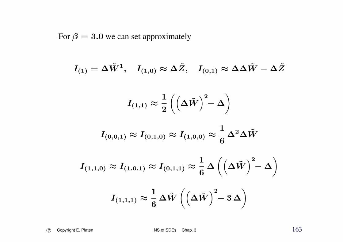
For β = 3.0 we can set approximately
I(1) = ∆W 1, I(1,0) ≈ ∆Z, I(0,1) ≈ ∆∆W − ∆Z
I(1,1) ≈1
2
((∆W
)2− ∆
)
I(0,0,1) ≈ I(0,1,0) ≈ I(1,0,0) ≈1
6∆2∆W
I(1,1,0) ≈ I(1,0,1) ≈ I(0,1,1) ≈1
6∆
((∆W
)2− ∆
)
I(1,1,1) ≈1
6∆W
((∆W
)2− 3∆
)
c⃝ Copyright E. Platen NS of SDEs Chap. 3 163

where ∆W and ∆Z
are correlated Gaussian random variables
c⃝ Copyright E. Platen NS of SDEs Chap. 3 164

Hofmann (1994)
=⇒ additive noise, β = 3.0, m ∈ 1, 2, . . .
I(0) = ∆, I(j) = ξj√∆, I(0,0) =
∆2
2, I(0,0,0) =
∆3
6
I(j,0) ≈1
2
(ξj + φj
1√3∆
)∆
32 , I(j,0,0) ≈ I(0,j,0) ≈
∆52
6ξj
I(j1,j2,0) ≈∆2
6
(ξj1 ξj2 +
Vj1,j2
∆
)
independent four point distributed random variables
ξ1, . . . , ξm
c⃝ Copyright E. Platen NS of SDEs Chap. 3 165

P
(ξj = ±
√3 +
√6
)=
1
12 + 4√6
P
(ξj = ±
√3 −
√6
)=
1
12 − 4√6
independent three point distributed random variables
φ1, . . . , φm
independent two-point distributed random variables
Vj1,j2
c⃝ Copyright E. Platen NS of SDEs Chap. 3 166

• multi-dimensional case
d, m ∈ 1, 2, . . .
additive noise
weak order 3.0 Taylor scheme
c⃝ Copyright E. Platen NS of SDEs Chap. 3 167

Y kn+1 = Y k
n + ak ∆ +
m∑j=1
bk,j ∆W j +1
2L0ak ∆2 +
1
6L0L0ak ∆3
+
m∑j=1
(Ljak ∆Zj + L0bk,j
(∆W j∆ − ∆Zj
)
+1
6
(L0L0bk,j + L0Ljak + LjL0ak
)∆W j ∆2
)
+1
6
m∑j1,j2=1
Lj1Lj2ak(∆W j1∆W j2 − Ij1=j2 ∆
)∆
c⃝ Copyright E. Platen NS of SDEs Chap. 3 168

∆W j and ∆Zj
independent pairs of
correlated Gaussian random variables
c⃝ Copyright E. Platen NS of SDEs Chap. 3 169

Weak Order 4.0 Taylor Scheme
Wagner-Platen expansion =⇒
• weak order 4.0 Taylor scheme
d, m ∈ 1, 2, . . .
Y kn+1 = Y k
n +4∑
ℓ=1
m∑j1,...,jℓ=0
Lj1 · · ·Ljℓ−1 bk,jℓ I(j1,...,jℓ)
β = 4.0
Pl. (1984)
c⃝ Copyright E. Platen NS of SDEs Chap. 3 170

• simplified weak order 4.0 Taylor scheme for additive noise
Yn+1 = Yn + a∆ + b∆W +1
2L0a∆2 + L1a∆Z
+L0b(∆W ∆ − ∆Z
)+
1
3!
(L0L0b + L0L1a
)∆W ∆2
+L1L1a
(2∆W ∆Z −
5
6
(∆W
)2∆ −
1
6∆2
)
+1
3!L0L0a∆3 +
1
4!L0L0L0a∆4
c⃝ Copyright E. Platen NS of SDEs Chap. 3 171

+1
4!
(L1L0L0a + L0L1L0a + L0L0L1a + L0L0L0b
)∆W ∆3
+1
4!
(L1L1L0a + L0L1L1a + L1L0L1a
) ((∆W
)2− ∆
)∆2
+1
4!L1L1L1a∆W
((∆W
)2− 3∆
)∆
∆W ∼ N(0,∆), ∆Z ∼ N(0,1
3∆3)
E(∆W ∆Z) =1
2∆2
c⃝ Copyright E. Platen NS of SDEs Chap. 3 172

A Simulation Study
• SDE with additive noise
dXt = aXt dt + b dWt
X0 = 1, a = 1.5, b = 0.01 and T = 1
g(X) = x
c⃝ Copyright E. Platen NS of SDEs Chap. 3 173

-5 -4 -3 -2 -1 0
Log2-dt
-20
-15
-10
-5
0
Log2-WeakErrors
Weak Error
4Taylor
3Taylor
2Taylor
Euler
Figure 3.5: Log-log plot of the weak error for an SDE with additive noiseusing weak Taylor schemes.
c⃝ Copyright E. Platen NS of SDEs Chap. 3 174

• SDE with multiplicative noise
dXt = aXt dt + bXt dWt
g(X) = x
c⃝ Copyright E. Platen NS of SDEs Chap. 3 175

-5 -4 -3 -2 -1 0
Log2-dt
-15
-10
-5
0
Log2-WeakErrors
Weak Error
4Taylor
3Taylor
2Taylor
Euler
Figure 3.6: Log-log plot of the weak error for an SDE with multiplicativenoise using weak Taylor schemes.
c⃝ Copyright E. Platen NS of SDEs Chap. 3 176

Convergence Theorem
• Wagner-Platen expansion
• Ito coefficient functions
f(t, x) ≡ x
fα(t, x) = Lj1 · · ·Ljℓ−1 bjℓ(x)
α = (j1, . . . , jℓ) ∈Mm, m ∈ 1, 2, . . .
c⃝ Copyright E. Platen NS of SDEs Chap. 3 177
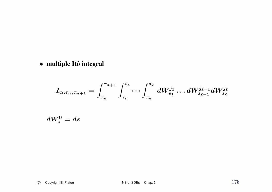
• multiple Ito integral
Iα,τn,τn+1=
∫ τn+1
τn
∫ sℓ
τn
· · ·∫ s2
τn
dW j1s1
. . . dW jℓ−1sℓ−1
dW jℓsℓ
dW 0s = ds
c⃝ Copyright E. Platen NS of SDEs Chap. 3 178
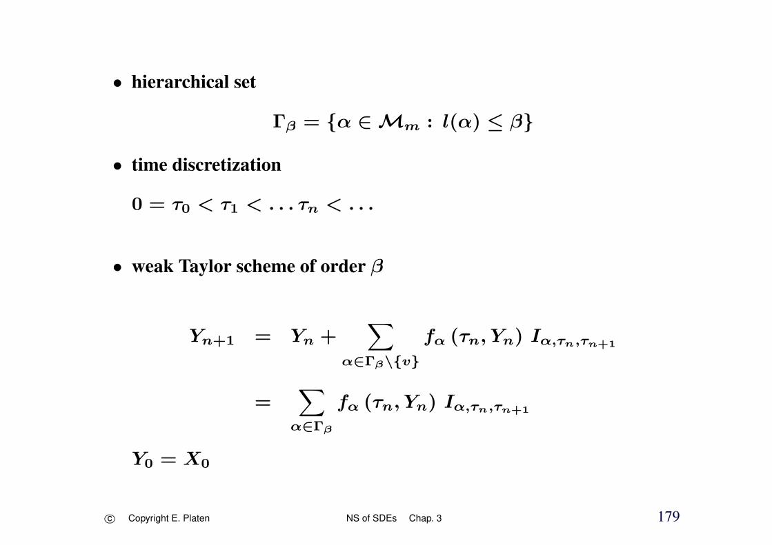
• hierarchical set
Γβ = α ∈ Mm : l(α) ≤ β
• time discretization
0 = τ0 < τ1 < . . . τn < . . .
• weak Taylor scheme of order β
Yn+1 = Yn +∑
α∈Γβ\v
fα (τn, Yn) Iα,τn,τn+1
=∑
α∈Γβ
fα (τn, Yn) Iα,τn,τn+1
Y0 = X0
c⃝ Copyright E. Platen NS of SDEs Chap. 3 179

Theorem
For some β ∈ 1, 2, . . . and autonomous X let Y ∆ be a weak Taylorscheme of order β. Suppose that a and b are Lipschitz continuous withcomponents ak, bk,j ∈ C2(β+1)
P
(ℜd,ℜ
)for all k ∈ 1, 2, . . . , d and
j ∈ 0, 1, . . . ,m, and that the fα satisfy a linear growth bound
|fα(t, x)| ≤ K (1 + |x|) ,
for all α ∈ Γβ, x ∈ℜd and t ∈ [0, T ], where K <∞. Then for each g ∈
C2(β+1)P
(ℜd,ℜ
)there exists a constant Cg , which does not depend on ∆,
such that
µ(∆) =∣∣E (g (XT )) − E
(g(Y ∆T
))∣∣ ≤ Cg ∆β,
that is Y ∆ converges with weak order β to X at time T as ∆ → 0.
c⃝ Copyright E. Platen NS of SDEs Chap. 3 180

Derivative Free Weak Approximations
Explicit Weak Order 2.0 Scheme
• explicit weak order 2.0 scheme
m = 1 and d ∈ 1, 2, . . .
Yn+1 = Yn +1
2
(a(Υ)+ a
)∆
+1
4
(b(Υ+
)+ b
(Υ−)+ 2b
)∆W
+1
4
(b(Υ+
)− b
(Υ−)) ((∆W
)2− ∆
)∆
12
c⃝ Copyright E. Platen NS of SDEs Chap. 3 181

with supporting values
Υ = Yn + a∆ + b∆W
and
Υ± = Yn + a∆ ± b√∆
∆W Gaussian or three-point distributed
P(∆W = ±
√3∆)=
1
6and P
(∆W = 0
)=
2
3
c⃝ Copyright E. Platen NS of SDEs Chap. 3 182

• multi-dimensional explicit weak order 2.0 scheme
d, m ∈ 1, 2, . . .
Yn+1 = Yn +1
2
(a(Υ)+ a
)∆
+1
4
m∑j=1
[ (bj(Rj
+
)+ bj
(Rj
−
)+ 2bj
)∆W j
+m∑
r=1r =j
(bj(Ur
+
)+ bj
(Ur
−
)− 2bj
)∆W j ∆− 1
2
]
c⃝ Copyright E. Platen NS of SDEs Chap. 3 183

+1
4
m∑j=1
[(bj(Rj
+
)− bj
(Rj
−
))((∆W j
)2− ∆
)
+m∑
r=1r =j
(bj(Ur
+
)− bj
(Ur
−
))(∆W j∆W r + Vr,j
)]∆− 1
2
c⃝ Copyright E. Platen NS of SDEs Chap. 3 184

with supporting values
Υ = Yn + a∆ +m∑
j=1
bj ∆W j, Rj± = Yn + a∆ ± bj
√∆
andU j
± = Yn ± bj√∆
∆W j and Vr,j as before
c⃝ Copyright E. Platen NS of SDEs Chap. 3 185

• additive noise
=⇒
Yn+1 = Yn +1
2
a
(Yn + a∆ +
m∑j=1
bj ∆W j
)+ a
∆
+m∑
j=1
bj ∆W j
c⃝ Copyright E. Platen NS of SDEs Chap. 3 186

Explicit Weak Order 3.0 Schemes
• explicit weak order 3.0 scheme
d ∈ 1, 2, . . . with m = 1
Yn+1 = Yn + a∆ + b∆W +1
2
(a+ζ + a−
ζ −3
2a −
1
4
(a+ζ + a−
ζ
))∆
+
√2
∆
(1√2
(a+ζ − a−
ζ
)−
1
4
(a+ζ − a−
ζ
))ζ ∆Z
+1
6
[a(Yn +
(a + a+
ζ
)∆ + (ζ + ϱ) b
√∆)− a+
ζ − a+ϱ + a
]×[(ζ + ϱ) ∆W
√∆ + ∆ + ζ ϱ
((∆W
)2− ∆
)]
c⃝ Copyright E. Platen NS of SDEs Chap. 3 187
witha±ϕ = a
(Yn + a∆ ± b
√∆ϕ
)and
a±ϕ = a
(Yn + 2a∆ ± b
√2∆ϕ
)
∆W ∼N(0,∆) and ∆Z ∼N(0, 13∆3)
E(∆W∆Z) =1
2∆2
P (ζ = ±1) = P (ϱ = ±1) =1
2
c⃝ Copyright E. Platen NS of SDEs Chap. 3 188

• explicit weak order 3.0 scheme for scalar noise
Yn+1 = Yn + a∆ + b∆W +1
2Ha ∆ +
1
∆Hb ∆Z
+
√2
∆Ga ζ ∆Z +
1√2∆
Gb ζ
((∆W
)2− ∆
)
+1
6F++a
(∆ + (ζ + ϱ)
√∆∆W + ζϱ
((∆W
)2− ∆
))+
1
24
(F++b + F−+
b + F+−b + F−−
b
)∆W
c⃝ Copyright E. Platen NS of SDEs Chap. 3 189
+1
24√∆
(F++b − F−+
b + F+−b − F−−
b
)((∆W
)2− ∆
)ζ
+1
24∆
(F++b + F−−
b − F−+b − F+−
b
)((∆W
)2− 3
)∆W ζϱ
+1
24√∆
(F++b + F−+
b − F+−b − F−−
b
)((∆W
)2− ∆
)ϱ
c⃝ Copyright E. Platen NS of SDEs Chap. 3 190

with
Hg = g+ + g− −3
2g −
1
4
(g+ + g−) ,
Gg =1√2
(g+ − g−)− 1
4
(g+ − g−) ,
F+±g = g
(Yn +
(a + a+
)∆ + b ζ
√∆ ± b+ ϱ
√∆)− g+
− g(Yn + a∆ ± b ϱ
√∆)+ g
c⃝ Copyright E. Platen NS of SDEs Chap. 3 191
F−±g = g
(Yn +
(a + a−)∆ − b ζ
√∆ ± b− ϱ
√∆)− g−
−g(Yn + a∆ ± b ϱ
√∆)+ g
where
g± = g(Yn + a∆ ± b ζ
√∆)
and
g± = g(Yn + 2 a∆ ±
√2 b ζ
√∆)
with g being equal to either a or b.
c⃝ Copyright E. Platen NS of SDEs Chap. 3 192
Extrapolation Methods
Weak Order 2.0 Extrapolation
• equidistant time discretizations
• simulate functional
E(g(Y ∆T
))using Euler scheme
with step size ∆
• repeat with the double step size 2∆
c⃝ Copyright E. Platen NS of SDEs Chap. 3 193

=⇒E(g(Y 2∆T
))
c⃝ Copyright E. Platen NS of SDEs Chap. 3 194

• combine these two functionals
=⇒
• weak order 2.0 extrapolation
V ∆g,2(T ) = 2E
(g(Y ∆T
))− E
(g(Y 2∆T
))
Talay & Tubaro (1990)
Richardson extrapolation
c⃝ Copyright E. Platen NS of SDEs Chap. 3 195

• example
geometric Brownian motion
dXt = aXt dt + bXt dWt
X0 = 0.1, a = 1.5 and b = 0.01
Richardson extrapolation V ∆g,2(T )
g(x) = x
=⇒ absolute weak error
µ(∆) =∣∣∣V ∆
g,2(T ) − E (g (XT ))∣∣∣
β = 2.0
c⃝ Copyright E. Platen NS of SDEs Chap. 3 196

-12
-11
-10
-9
-8
-7
-6
-6 -5.5 -5 -4.5 -4 -3.5 -3
time
Figure 3.7: Log-log plot for absolute weak error of Richardson extrapolationagainst step size.
c⃝ Copyright E. Platen NS of SDEs Chap. 3 197

Higher Weak Order Extrapolation
• weak order 4.0 extrapolation
V ∆g,4(T ) =
1
21
[32E
(g(Y ∆T
))− 12E
(g(Y 2∆T
))+ E
(g(Y 4∆T
)) ]
c⃝ Copyright E. Platen NS of SDEs Chap. 3 198

-13
-12
-11
-10
-9
-8
-7
-6
-5
-4
-3
-4 -3.5 -3 -2.5 -2
time
Figure 3.8: Log-log plot for absolute weak error of weak order 4.0 extra-polation.
c⃝ Copyright E. Platen NS of SDEs Chap. 3 199

Implicit and Predictor Corrector Methods
• numerical stability has highest priority
Drift Implicit Euler Scheme
d, m ∈ 1, 2, . . .
Yn+1 = Yn + a (τn+1, Yn+1)∆ +m∑
j=1
bj (τn, Yn)∆W j
P(∆W j = ±
√∆)=
1
2
c⃝ Copyright E. Platen NS of SDEs Chap. 3 200
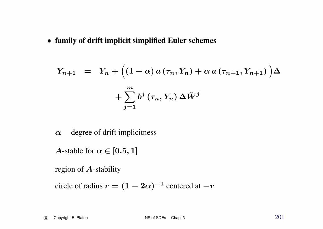
• family of drift implicit simplified Euler schemes
Yn+1 = Yn +((1 − α) a (τn, Yn) + αa (τn+1, Yn+1)
)∆
+m∑
j=1
bj (τn, Yn)∆W j
α degree of drift implicitness
A-stable for α ∈ [0.5, 1]
region of A-stability
circle of radius r = (1 − 2α)−1 centered at −r
c⃝ Copyright E. Platen NS of SDEs Chap. 3 201
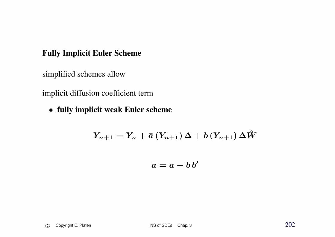
Fully Implicit Euler Scheme
simplified schemes allow
implicit diffusion coefficient term
• fully implicit weak Euler scheme
Yn+1 = Yn + a (Yn+1)∆ + b (Yn+1)∆W
a = a − b b′
c⃝ Copyright E. Platen NS of SDEs Chap. 3 202

• family of implicit weak Euler schemes
Yn+1 = Yn +(α aη (τn+1, Yn+1) + (1 − α) aη (τn, Yn)
)∆
+m∑
j=1
(η bj (τn+1, Yn+1) + (1 − η) bj (τn, Yn)
)∆W j
aη = a − ηm∑
j1,j2=1
d∑k=1
bk,j1∂bj2
∂xk
for α, η ∈ [0, 1]
c⃝ Copyright E. Platen NS of SDEs Chap. 3 203

Implicit Weak Order 2.0 Taylor Scheme
Yn+1 = Yn + a (Yn+1)∆ + b∆W
−1
2
(a (Yn+1) a
′ (Yn+1) +1
2b2 (Yn+1) a
′′ (Yn+1)
)∆2
+1
2b b′
((∆W
)2− ∆
)
+1
2
(−a′ b + a b′ +
1
2b′′b2
)∆W ∆
P(∆W = ±
√3∆)=
1
6and P
(∆W = 0
)=
2
3
Milstein (1995)
c⃝ Copyright E. Platen NS of SDEs Chap. 3 204

• family of implicit weak order 2.0 Taylor schemes
Yn+1 = Yn +(αa (τn+1, Yn+1) + (1 − α) a
)∆
+1
2
m∑j1,j2=1
Lj1bj2(∆W j1∆W j2 + Vj1,j2
)
+m∑
j=1
(bj +
1
2
(L0bj + (1 − 2α)Lja
)∆
)∆W j
+1
2(1 − 2α)
(β L0a + (1 − β)L0a (τn+1, Yn+1)
)∆2
α = 0.5 =⇒
c⃝ Copyright E. Platen NS of SDEs Chap. 3 205

Yn+1 = Yn +1
2
(a (τn+1, Yn+1) + a
)∆
+m∑
j=1
bj ∆W j +1
2
m∑j=1
L0bj ∆W j ∆
+1
2
m∑j1,j2=1
Lj1bj2(∆W j1∆W j2 + Vj1,j2
)
c⃝ Copyright E. Platen NS of SDEs Chap. 3 206

Implicit Weak Order 2.0 Scheme
m = 1
Pl. (1995)
• implicit weak order 2.0 scheme
Yn+1 = Yn +1
2(a + a (Yn+1))∆
+1
4
(b(Υ+
)+ b
(Υ−)+ 2 b
)∆W
+1
4
(b(Υ+
)− b
(Υ−)) ((∆W
)2− ∆
)∆− 1
2
c⃝ Copyright E. Platen NS of SDEs Chap. 3 207

with supporting values
Υ± = Yn + a∆ ± b√∆
∆W can be chosen as before
c⃝ Copyright E. Platen NS of SDEs Chap. 3 208

• implicit weak order 2.0 scheme
d, m ∈ 1, 2, . . .
c⃝ Copyright E. Platen NS of SDEs Chap. 3 209

Yn+1 = Yn +1
2(a + a (Yn+1))∆
+1
4
m∑j=1
[bj(Rj
+
)+ bj
(Rj
−
)+ 2bj
+
m∑r=1r =j
(bj(Ur
+
)+ bj
(Ur
−
)− 2bj
)∆− 1
2
]∆W j
+1
4
m∑j=1
[(bj(Rj
+
)− bj
(Rj
−
)) ((∆W j
)2− ∆
)
+m∑
r=1r =j
(bj(Ur
+
)− bj
(Ur
−
))(∆W j∆W r + Vr,j
)]∆− 1
2
c⃝ Copyright E. Platen NS of SDEs Chap. 3 210

supporting values
Rj± = Yn + a∆ ± bj
√∆
andU j
± = Yn ± bj√∆
A-stable
β = 2.0
c⃝ Copyright E. Platen NS of SDEs Chap. 3 211
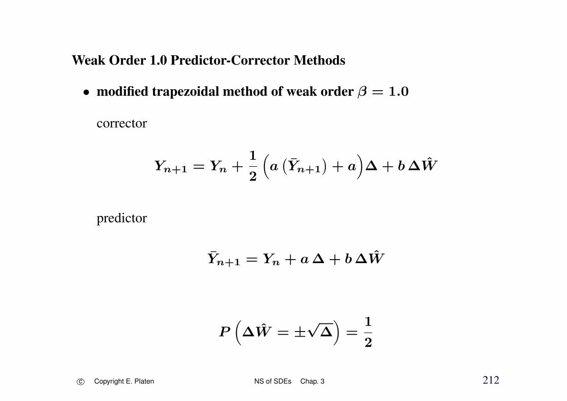
Weak Order 1.0 Predictor-Corrector Methods
• modified trapezoidal method of weak order β = 1.0
corrector
Yn+1 = Yn +1
2
(a(Yn+1
)+ a
)∆ + b∆W
predictor
Yn+1 = Yn + a∆ + b∆W
P(∆W = ±
√∆)=
1
2
c⃝ Copyright E. Platen NS of SDEs Chap. 3 212
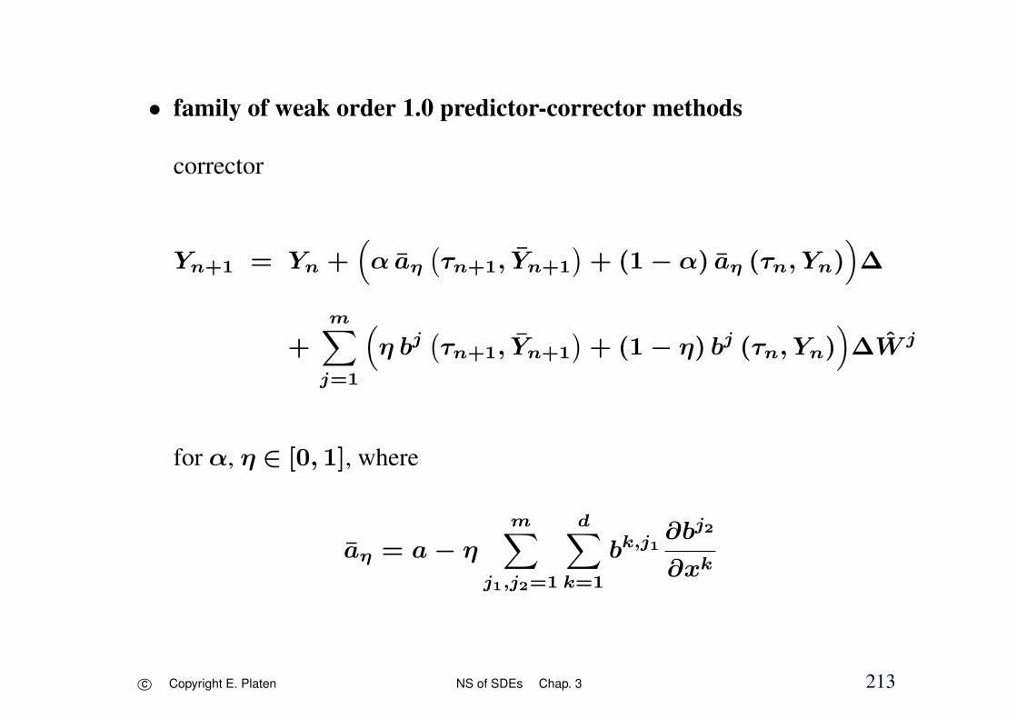
• family of weak order 1.0 predictor-corrector methods
corrector
Yn+1 = Yn +(α aη
(τn+1, Yn+1
)+ (1 − α) aη (τn, Yn)
)∆
+
m∑j=1
(η bj
(τn+1, Yn+1
)+ (1 − η) bj (τn, Yn)
)∆W j
for α, η ∈ [0, 1], where
aη = a − η
m∑j1,j2=1
d∑k=1
bk,j1∂bj2
∂xk
c⃝ Copyright E. Platen NS of SDEs Chap. 3 213

and predictor
Yn+1 = Yn + a∆ +m∑
j=1
bj ∆W j
c⃝ Copyright E. Platen NS of SDEs Chap. 3 214

Weak Order 2.0 Predictor-Corrector Methods
• weak order 2.0 predictor-corrector method
corrector
Yn+1 = Yn +1
2
(a(Yn+1
)+ a
)∆ + Ψn
with
Ψn = b∆W +1
2b b′
((∆W
)2− ∆
)
+1
2
(a b′ +
1
2b2 b′′
)∆W ∆
c⃝ Copyright E. Platen NS of SDEs Chap. 3 215

and as predictor
Yn+1 = Yn + a∆ + Ψn
+1
2a′ b∆W ∆ +
1
2
(a a′ +
1
2a′′b2
)∆2
P(∆W = ±
√3∆)=
1
6and P
(∆W = 0
)=
2
3
c⃝ Copyright E. Platen NS of SDEs Chap. 3 216

• general multi-dimensional case
corrector
Yn+1 = Yn +1
2
(a(τn+1, Yn+1
)+ a
)∆ + Ψn
where
Ψn =m∑
j=1
(bj +
1
2L0bj∆
)∆W j
+1
2
m∑j1,j2=1
Lj1bj2(∆W j1 ∆W j2 + Vj1,j2
)and predictor
Yn+1 = Yn + a∆ + Ψn +1
2L0a∆2 +
1
2
m∑j=1
Lja∆W j ∆
c⃝ Copyright E. Platen NS of SDEs Chap. 3 217

• derivative free weak order 2.0 predictor-corrector method
corrector
Yn+1 = Yn +1
2
(a(Yn+1
)+ a
)∆ + ϕn
where
ϕn =1
4
(b(Υ+
)+ b
(Υ−)+ 2 b
)∆W
+1
4
(b(Υ+
)− b
(Υ−)) ((∆W
)2− ∆
)∆− 1
2
with supporting values
Υ± = Yn + a∆ ± b√∆
c⃝ Copyright E. Platen NS of SDEs Chap. 3 218

and with predictor
Yn+1 = Yn +1
2
(a(Υ)+ a
)∆ + ϕn
with the supporting value
Υ = Yn + a∆ + b∆W
c⃝ Copyright E. Platen NS of SDEs Chap. 3 219

• multi-dimensional generalization
corrector
Yn+1 = Yn +1
2
(a(Yn+1
)+ a
)∆ + ϕn
c⃝ Copyright E. Platen NS of SDEs Chap. 3 220

where
ϕn =1
4
m∑j=1
[bj(Rj
+
)+ b
(Rj
−
)+ 2 bj
+m∑
r=1r =j
(bj(Ur
+
)+ b
(Ur
−
)− 2 bj
)∆− 1
2
]∆W j
+1
4
m∑j=1
[ (bj(Rj
+
)− b
(Rj
−
))((∆W
)2− ∆
)
+
m∑r=1r =j
(bj(Ur
+
)− b
(Ur
−
))(∆W j ∆W r + Vr,j
)]∆− 1
2
c⃝ Copyright E. Platen NS of SDEs Chap. 3 221

supporting values
Rj± = Yn + a∆ ± bj
√∆ and U j
± = Yn ± bj√∆
c⃝ Copyright E. Platen NS of SDEs Chap. 3 222

predictor
Yn+1 = Yn +1
2
(a(Υ)+ a
)∆ + ϕn
supporting value
Υ = Yn + a∆ +
m∑j=1
bj ∆W j
local error
Zn+1 = Yn+1 − Yn+1
c⃝ Copyright E. Platen NS of SDEs Chap. 3 223

4 Numerical Stability
• roundoff and truncation errors
• propagation of errors
• numerical stability priority over higher order
c⃝ Copyright E. Platen NS of SDEs Chap. 4 224

• specially designed test equations
Hernandez & Spigler (1992, 1993)
Milstein (1995)
Kloeden & Pl. (1992b)
Saito & Mitsui(1993a, 1993b, 1996)
Hofmann & Pl. (1994, 1996)
Higham (2000)
c⃝ Copyright E. Platen NS of SDEs Chap. 4 225

• linear test dynamics
Xt = X0 exp(1 − α)λ t +
√α |λ|Wt
α, λ ∈ ℜ
=⇒
P(limt→∞
Xt = 0)= 1 ⇐⇒ (1 − α)λ < 0
c⃝ Copyright E. Platen NS of SDEs Chap. 4 226

• linear Ito SDE
dXt =
(1 −
3
2α
)λXt dt +
√α |λ|Xt dWt
• corresponding Stratonovich SDE
dXt = (1 − α)λXt dt +√α |λ|Xt dWt
• α = 0 no randomness
• α = 23
Ito SDE no drift =⇒ martingale
• α = 1 Stratonovich SDE no drift
c⃝ Copyright E. Platen NS of SDEs Chap. 4 227

Definition 4.1 Y = Yt, t ≥ 0 is called asymptotically stable if
P(limt→∞
|Yt| = 0)= 1.
impact of perturbations declines asymptotically over time
c⃝ Copyright E. Platen NS of SDEs Chap. 4 228

• stability region Γ
those pairs (λ∆, α) ∈ (−∞, 0)× [0, 1) for which approximation Y
asymptotically stable
c⃝ Copyright E. Platen NS of SDEs Chap. 4 229

• transfer function
∣∣∣∣Yn+1
Yn
∣∣∣∣ = Gn+1(λ∆, α)
Y asymptotically stable ⇐⇒
E(ln(Gn+1(λ∆, α))) < 0
Higham (2000)
c⃝ Copyright E. Platen NS of SDEs Chap. 4 230
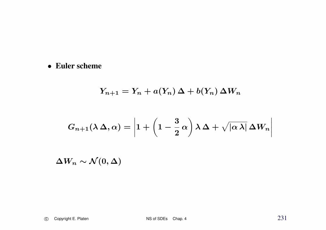
• Euler scheme
Yn+1 = Yn + a(Yn)∆ + b(Yn)∆Wn
Gn+1(λ∆, α) =
∣∣∣∣1 +
(1 −
3
2α
)λ∆ +
√|αλ|∆Wn
∣∣∣∣∆Wn ∼ N (0,∆)
c⃝ Copyright E. Platen NS of SDEs Chap. 4 231

Figure 4.1: A-stability region for the Euler scheme.
c⃝ Copyright E. Platen NS of SDEs Chap. 4 232
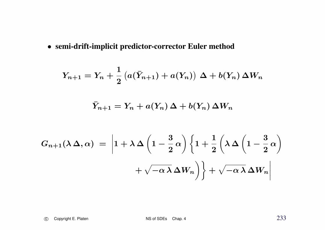
• semi-drift-implicit predictor-corrector Euler method
Yn+1 = Yn +1
2
(a(Yn+1) + a(Yn)
)∆ + b(Yn)∆Wn
Yn+1 = Yn + a(Yn)∆ + b(Yn)∆Wn
Gn+1(λ∆, α) =
∣∣∣∣1 + λ∆
(1 −
3
2α
)1 +
1
2
(λ∆
(1 −
3
2α
)
+√−αλ∆Wn
)+√−αλ∆Wn
∣∣∣∣
c⃝ Copyright E. Platen NS of SDEs Chap. 4 233

Figure 4.2: A-stability region for semi-drift-implicit predictor-corrector Eu-ler method.
c⃝ Copyright E. Platen NS of SDEs Chap. 4 234

• drift-implicit predictor-corrector Euler method
Yn+1 = Yn + a(Yn+1)∆ + b(Yn)∆Wn
Yn+1 = Yn + a(Yn)∆ + b(Yn)∆Wn
Gn+1(λ∆, α) =
∣∣∣∣1 + λ∆
(1 −
3
2α
)1 + λ∆
(1 −
3
2α
)
+√−αλ∆Wn
+√
−αλ∆Wn
∣∣∣∣
c⃝ Copyright E. Platen NS of SDEs Chap. 4 235

Figure 4.3: A-stability region for drift-implicit predictor-corrector Eulermethod.
c⃝ Copyright E. Platen NS of SDEs Chap. 4 236
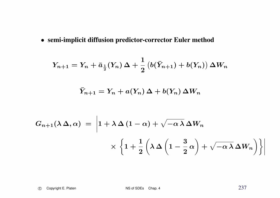
• semi-implicit diffusion predictor-corrector Euler method
Yn+1 = Yn + a 12(Yn)∆ +
1
2
(b(Yn+1) + b(Yn)
)∆Wn
Yn+1 = Yn + a(Yn)∆ + b(Yn)∆Wn
Gn+1(λ∆, α) =
∣∣∣∣1 + λ∆(1 − α) +√−αλ∆Wn
×1 +
1
2
(λ∆
(1 −
3
2α
)+√−αλ∆Wn
)∣∣∣∣
c⃝ Copyright E. Platen NS of SDEs Chap. 4 237

Figure 4.4: A-stability region for the predictor-corrector Euler method withθ = 0 and η = 1
2.
c⃝ Copyright E. Platen NS of SDEs Chap. 4 238

• symmetric predictor-corrector Euler method
Yn+1 = Yn+1
2
(a 1
2(Yn+1) + a 1
2(Yn)
)∆+
1
2
(b(Yn+1) + b(Yn)
)∆Wn
Yn+1 = Yn + a(Yn)∆ + b(Yn)∆Wn
Gn+1(λ∆, α) =
∣∣∣∣1 + λ∆(1 − α)
1 +
1
2
(λ∆
(1 −
3
2α
)+√−αλ∆Wn
)
+√
−αλ∆Wn
1 +
1
2
(λ∆
(1 −
3
2α
)+√−αλ∆Wn
)∣∣∣∣
c⃝ Copyright E. Platen NS of SDEs Chap. 4 239

Figure 4.5: A-stability region for the symmetric predictor-corrector Eulermethod.
c⃝ Copyright E. Platen NS of SDEs Chap. 4 240

Gn+1(λ∆, α) =
∣∣∣∣1 + λ∆
(1 −
1
2α
)1 + λ∆
(1 −
3
2α
)+√
−αλ∆Wn
+√−αλ∆Wn
1 + λ∆
(1 −
3
2α
)+√−αλ∆Wn
∣∣∣∣=
∣∣∣∣1 +
1 + λ∆
(1 −
3
2α
)+√−αλ∆Wn
×λ∆
(1 −
1
2α
)+√−αλ∆Wn
∣∣∣∣
c⃝ Copyright E. Platen NS of SDEs Chap. 4 241

Figure 4.6: A-stability region for fully implicit predictor-corrector Eulermethod.
c⃝ Copyright E. Platen NS of SDEs Chap. 4 242

0
5
10
15
20
25
30
35
40
0 0.05 0.1 0.15 0.2 0.25 0.3 0.35 0.4 0.45 0.5
time
exact solutionpredictor corrector
Figure 4.7: Exact solution and approximate solution generated by the sym-metric predictor-corrector Euler scheme.
c⃝ Copyright E. Platen NS of SDEs Chap. 4 243

p-Stability
Pl. & Shi (2008)
Definition 4.2 For p > 0 a process Y = Yt, t > 0 is called p-stableif
limt→∞
E(|Yt|p) = 0.
For α ∈ [0, 11+p/2
) and λ < 0 test SDE is p-stable.
c⃝ Copyright E. Platen NS of SDEs Chap. 4 244

• Stability region those triplets (λ∆, α, p) for which Y is p-stable.
c⃝ Copyright E. Platen NS of SDEs Chap. 4 245

For λ∆ < 0, α ∈ [0, 1) and p > 0 Y p-stable ⇐⇒
E((Gn+1(λ∆, α))p) < 1
• for p > 0
=⇒
E(ln(Gn+1(λ∆, α))) ≤1
pE((Gn+1(λ∆, α))p − 1) < 0
=⇒ asymptotically stable
c⃝ Copyright E. Platen NS of SDEs Chap. 4 246

Figure 4.8: Stability region for the Euler scheme.
c⃝ Copyright E. Platen NS of SDEs Chap. 4 247
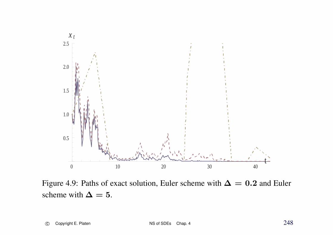
0 10 20 30 40t
0.5
1.0
1.5
2.0
2.5x t
Figure 4.9: Paths of exact solution, Euler scheme with ∆ = 0.2 and Eulerscheme with ∆ = 5.
c⃝ Copyright E. Platen NS of SDEs Chap. 4 248

Figure 4.10: Stability region for semi-drift-implicit predictor-corrector Eulermethod.
c⃝ Copyright E. Platen NS of SDEs Chap. 4 249

Figure 4.11: Stability region for drift-implicit predictor-corrector Eulermethod.
c⃝ Copyright E. Platen NS of SDEs Chap. 4 250

Figure 4.12: Stability region for the predictor-corrector Euler method withθ = 0 and η = 1
2.
c⃝ Copyright E. Platen NS of SDEs Chap. 4 251

Figure 4.13: Stability region for the symmetric predictor-corrector Eulermethod.
c⃝ Copyright E. Platen NS of SDEs Chap. 4 252

Figure 4.14: Stability region for fully implicit predictor-corrector Eulermethod.
c⃝ Copyright E. Platen NS of SDEs Chap. 4 253
Stability of Some Implicit Methods
• semi-drift implicit Euler scheme
Yn+1 = Yn +1
2(a(Yn+1) + a(Yn))∆ + b(Yn)∆Wn
• full-drift implicit Euler scheme
Yn+1 = Yn + a(Yn+1)∆ + b(Yn)∆Wn
solve algebraic equation
c⃝ Copyright E. Platen NS of SDEs Chap. 4 254

Figure 4.15: Stability region for semi-drift implicit Euler method.
c⃝ Copyright E. Platen NS of SDEs Chap. 4 255

Figure 4.16: Stability region for full-drift implicit Euler method.
c⃝ Copyright E. Platen NS of SDEs Chap. 4 256

• balanced implicit Euler method
Milstein, Pl. & Schurz (1998)
Yn+1 = Yn+
(1 −
3
2α
)λYn∆+
√α|λ|Yn∆Wn+c|∆Wn|(Yn−Yn+1)
c⃝ Copyright E. Platen NS of SDEs Chap. 4 257

Figure 4.17: Stability region for a balanced implicit Euler method.
c⃝ Copyright E. Platen NS of SDEs Chap. 4 258

Figure 4.18: Stability region for the simplified symmetric Euler method.
c⃝ Copyright E. Platen NS of SDEs Chap. 4 259

Figure 4.19: Stability region for the simplified symmetric implicit EulerScheme.
c⃝ Copyright E. Platen NS of SDEs Chap. 4 260

Figure 4.20: Stability region for the simplified fully implicit Euler Scheme.
c⃝ Copyright E. Platen NS of SDEs Chap. 4 261

5 Variance Reduction Techniques
Various Variance Reduction Methods
• classical
Hammersley & Handscomb (1964)Ermakov (1975), Boyle (1977)Maltz & Hitzl (1979), Rubinstein (1981)Ermakov & Mikhailov (1982), Ripley (1983)Kalos & Whitlock (1986), Bratley, Fox & Schrage (1987)Chang (1987),Wagner (1987)Law & Kelton (1991), Ross (1990)
c⃝ Copyright E. Platen NS of SDEs Chap. 5 262

• stochastic differential equations
Boyle (1977)Boyle, Broadie & Glasserman (1997)Broadie & Glasserman (1997), Fu (1995)Grant, Vora & Weeks (1997), Joy, Boyle & Tan (1996)Glasserman (2004)Longstaff & Schwartz (2001)Milstein (1988), Kloeden & Pl. (1992b)Hofmann, Pl. & Schweizer (1992), Heath (1995)Goldman, Heath, Kentwell & Pl. (1995)Fournie, Lasry & Touzi (1997)Newton (1994)
c⃝ Copyright E. Platen NS of SDEs Chap. 5 263

Antithetic Variates
• probability space
(Ω,AT ,A, P ) where Ω = C([t0, T ],ℜ2)
ω(t) = (ω1(t), ω2(t))⊤ ∈ ℜ2 for t ∈ [t0, T ]
• coordinate mappings
W 1t (ω) = ω1(t) and W 2
t (ω) = ω2(t)
dXt0,xt = a
(t,X
t0,xt
)dt + b
(t,X
t0,xt
)dWt
c⃝ Copyright E. Platen NS of SDEs Chap. 5 264

For ω ∈ Ω, define ω ∈ Ω by ω(t) = (−ω1(t),−ω2(t))⊤, t ∈
[t0, T ]
h(X
t0,xT
)(ω) = h
(X
t0,xT
)(ω)
• unbiased estimator
h(X
t0,xT
)=
1
2
(h(X
t0,xT
)+ h
(X
t0,xT
))=⇒
Var(h(X
t0,xT
))=
1
4
(Var
(h(X
t0,xT
))+ Var
(h(X
t0,xT
))+ 2 Cov
(h(X
t0,xT
), h(X
t0,xT
)))c⃝ Copyright E. Platen NS of SDEs Chap. 5 265
Stratified Sampling
• set of events
Ai ⊆ AT , i ∈ 1, 2, . . . , N
N∪i=1
Ai = Ω, Ai ∩ Aj = ∅
for i, j ∈ 1, 2, . . . , N, P (Ai) = 1N
A = σ Ai, i ∈ 1, 2, . . . , N
c⃝ Copyright E. Platen NS of SDEs Chap. 5 266

• random variable
Z : Ω → ℜ
• restriction of Z to Ai
ZAi(ω) = Z(ω) for ω ∈ Ai
c⃝ Copyright E. Platen NS of SDEs Chap. 5 267

• unbiased estimator for E(Z)
Z =1
N
N∑i=1
ZAi
where ZAi independent
E(Z) =1
N
N∑i=1
E(ZAi) =
N∑i=1
∫Ai
Z dP =
∫Ω
Z dP = E(Z)
independence
=⇒
c⃝ Copyright E. Platen NS of SDEs Chap. 5 268

Var(Z) =
N∑i=1
Var(ZAi)
N2
=1
NE(Var(Z
∣∣A))
≤1
NVar(Z)
c⃝ Copyright E. Platen NS of SDEs Chap. 5 269

Example: simplified weak Euler approximation Y ∆
∆Wk two-point distributed
two-point variates with N time steps
underlying sample space
=⇒ΩN = −1, 10,1,...,N−1
‘path’ for Wk
given by ∆Wk(ω) = ωk
√∆
probabilities PN(ω) = 12N
only a tiny fraction of these paths can be sampled
c⃝ Copyright E. Platen NS of SDEs Chap. 5 270

A stratified Monte Carlo estimation could consist of exhausting all pathsω ∈ ΩN up to time tN ′ and then sampling randomly;
reduces duplicate traversals of the early nodes of the lattice.
c⃝ Copyright E. Platen NS of SDEs Chap. 5 271
Measure Transformation Method
see Kloeden & Pl. (1992b)
• d-dimensional diffusion
dXs,xt = a(t,Xs,x
t ) dt +m∑
j=1
bj(t,Xs,xt ) dW j
t
on (Ω,AT ,A, P )
• approximate the functional
u(s, x) = E(g(Xs,x
T )∣∣As
)c⃝ Copyright E. Platen NS of SDEs Chap. 5 272

• Kolmogorov backward equation
L0 u(s, x) = 0
for (s, x) ∈ (0, T ) × ℜd with
u(T, y) = g(y)
L0 =∂
∂s+
d∑k=1
ak ∂
∂xk+
1
2
d∑k,ℓ=1
m∑j=1
bk,j bℓ,j∂2
∂xk ∂xℓ
c⃝ Copyright E. Platen NS of SDEs Chap. 5 273

• Girsanov transformation
W jt = W j
t −∫ t
0
dj(z, X0,x
z
)dz
dj denotes given, rather flexible real-valued function
• Radon-Nikodym derivative
dP
dP=
Θt
Θ0
c⃝ Copyright E. Platen NS of SDEs Chap. 5 274

• SDE
dX0,xt = a
(t, X0,x
t
)dt +
m∑j=1
bj(t, X0,x
t
)dW j
t
=
a(t, X0,x
t
)−
m∑j=1
bj(t, X0,x
t
)dj(t, X0,x
t
) dt
+m∑
j=1
bj(t, X0,x
t
)dW j
t
• Radon-Nikodym derivative process
Θt = Θ0 +m∑
j=1
∫ t
0
Θz dj(z, X0,x
z
)dW j
z
(A, P )-martingale
c⃝ Copyright E. Platen NS of SDEs Chap. 5 275

• diffusion process X0,x with respect to P
same drift and diffusion coefficients as Xs,x
=⇒
E(g(X0,x
T
))=
∫Ω
g(X0,x
T
)dP
=
∫Ω
g(X0,x
T
)dP
=
∫Ω
g(X0,x
T
) ΘT
Θ0
dP
= E
(g(X0,x
T
) ΘT
Θ0
)
c⃝ Copyright E. Platen NS of SDEs Chap. 5 276

• unbiased estimator
g(X0,x
T
) ΘT
Θ0
no particular choice of dj made so far
c⃝ Copyright E. Platen NS of SDEs Chap. 5 277

• ideally choose dj in the form
dj(t, x) = −1
u(t, x)
d∑k=1
bk,j(t, x)∂u(t, x)
∂xk
then it can be shown that
u(t, X0,x
t
)Θt = u(0, x)Θ0
for all t ∈ [0, T ]
=⇒u(0, x) = g
(X0,x
T
) ΘT
Θ0
c⃝ Copyright E. Platen NS of SDEs Chap. 5 278
=⇒
g(X0,x
T
) ΘT
Θ0
is not random
c⃝ Copyright E. Platen NS of SDEs Chap. 5 279

• guess a function u
dj(t, x) = −1
u(t, x)
d∑k=1
bk,j(t, x)∂u(t, x)
∂xk
• used unbiased estimator
g(X0,x
T
) ΘT
Θ0
E
(g(X0,x
T
) ΘT
Θ0
)= E
(g(X0,x
T
))
c⃝ Copyright E. Platen NS of SDEs Chap. 5 280
Control Variates and Integral Representations
Clewlow & Carverhill (1992, 1994)
Basic Control Variate Method
• valuation martingale
Mt = u(t,X
t0,xt
)= E
(h(X
t0,xT
) ∣∣∣ At
)
construct an accurate and fast estimate of
E(h(Xt0,xT )) = u(t0, x)
c⃝ Copyright E. Platen NS of SDEs Chap. 5 281

• control variate
find Y with known mean E(Y )
• unbiased estimator
Z = h(Xt0,xT ) − α(Y − E(Y ))
α ∈ ℜ
E(Z) = E(h(Xt0,xT ))
c⃝ Copyright E. Platen NS of SDEs Chap. 5 282

• known valuation function
u(t, X
t0,xt
)= E
(h(X
t0,xT
) ∣∣∣ At
)
Xt0,x approximates Xt0,xT
• unbiased estimator
ZT = h(X
t0,xT
)− α
(h(X
t0,xT
)− E
(h(X
t0,xT
)))= u
(T,X
t0,xT
)− α
(u(T, X
t0,xT
)− u(t0, x)
)
variance can be reduced
c⃝ Copyright E. Platen NS of SDEs Chap. 5 283

Var(ZT ) = Var(h(X
t0,xT
))+ α2 Var
(h(X
t0,xT
))− 2α Cov
(h(X
t0,xT
), h(X
t0,xT
))
minimize the variance
αmin =Cov
(h(X
t0,xT
), h(X
t0,xT
))Var
(h(X
t0,xT
))
c⃝ Copyright E. Platen NS of SDEs Chap. 5 284

Example: Stochastic Volatility
• SDE
dSt = σt St dW1t
dσt = (κ − σt) dt + ξ σt dW2t
(Ω,AT ,A, P )
• European call payoff
h(ST ) = (ST − K)+
c⃝ Copyright E. Platen NS of SDEs Chap. 5 285

• adjusted price process
dSt = σtSt dW1t
dσt = (κ − σt) dt
• adjusted valuation function
u(t, St, σt) = E((ST − K)+
∣∣∣At
)• unbiased variate
ZT = (ST − K)+ − α((ST − K)+ − E(ST − K)+)
= (ST − K)+ − α((ST − K)+ − u(t0, s, σ))
unbiased variance reduced estimator
c⃝ Copyright E. Platen NS of SDEs Chap. 5 286
Variance Reduction via Integral Representations
Heath & Pl. (2002)
The HP Variance Reduced Estimator
• SDE
dXs,xt = a(t,Xs,x
t ) dt +m∑
j=1
bj(t,Xs,xt ) dW j
t
• first exit time
τ = inft ≥ s : (t,Xs,xt ) ∈ [s, T ) × Γ
c⃝ Copyright E. Platen NS of SDEs Chap. 5 287

• operators
L0 f(t, x) =∂f(t, x)
∂t+
d∑i=1
ai(t, x)∂f(t, x)
∂xi
+1
2
d∑i,k=1
m∑j=1
bi,j(t, x) bk,j(t, x)∂2f(t, x)
∂xi ∂xk
and
Lj f(t, x) =d∑
i=1
bi,j(t, x)∂f(t, x)
∂xi
for (t, x) ∈ (0, T ) × Γ
c⃝ Copyright E. Platen NS of SDEs Chap. 5 288

• valuation function
u(t, x) = E(h(τ,Xt,x
τ ))
for (t, x) ∈ [0, T ] × Γ
assume
Mt = E(h(τ,X0,x
τ
) ∣∣At
)
square integrable (A, P )-martingale
c⃝ Copyright E. Platen NS of SDEs Chap. 5 289

martingale representation theorem
=⇒
Mt = u(t,X0,xt∧τ )
= u(0, x) +m∑
j=1
∫ t∧τ
0
ξjs dWjs
for t ∈ [0, T ]
c⃝ Copyright E. Platen NS of SDEs Chap. 5 290

• given an approximation
u : [0, T ] × Γ → ℜ to u
u ∈ C1,2([0, T ] × Γ)
with
M jt =
∫ t∧τ
0
Lj u(s,X0,xs ) dW j
s
square integrable (A, P )-martingale
c⃝ Copyright E. Platen NS of SDEs Chap. 5 291

u(τ,X0,xτ ) = u(τ,X0,x
τ ) = h(τ,X0,xτ )
=⇒
u(τ,X0,xτ ) = u(0, x) +
∫ τ
0
L0 u(t,X0,xt ) dt
+m∑
j=1
∫ τ
0
Lj u(t,X0,xt ) dW j
t
c⃝ Copyright E. Platen NS of SDEs Chap. 5 292

=⇒
u(0, x) = E(h(τ,X0,x
τ ))
= E(u(τ,X0,x
τ ))
= u(0, x) + E
(∫ τ
0
L0 u(t,X0,xt ) dt
)
= u(0, x) +
∫ T
0
E(1t<τL
0 u(t,X0,xt )
)dt
• unbiased estimator for u(0, x)
Zτ = u(0, x) +
∫ τ
0
L0 u(t,X0,xt ) dt
HP estimator
c⃝ Copyright E. Platen NS of SDEs Chap. 5 293

Variance of the HP Estimator
Zτ = u(τ,X0,xτ ) −
m∑j=1
∫ τ
0
Lj u(t,X0,xt ) dW j
t
= u(τ,X0,xτ ) −
m∑j=1
∫ τ
0
Lj u(t,X0,xt ) dW j
t
= u(0, x) +m∑
j=1
∫ τ
0
(ξjt − Lj u(t,X0,x
t ))dW j
t
=⇒
c⃝ Copyright E. Platen NS of SDEs Chap. 5 294

Var(Zτ ) = E
m∑
j=1
∫ τ
0
(ξjt − Lj u(t,X0,x
t ))dW j
t
2
=m∑
j=1
∫ T
0
E
(1t<τ
(ξjt − Lj u(t,X0,x
t ))2)
dt
c⃝ Copyright E. Platen NS of SDEs Chap. 5 295

• integrands
ξjt = Lj u(t,X0,xt )
=⇒
Var(Zτ ) =
m∑j=1
∫ T
0
E
(1t<τ
((Lj u − Lj u) (t,X0,x
t ))2)
dt
if a good approximation u to u can be found,
so that Lj u is close to Lj u
variance will be small
c⃝ Copyright E. Platen NS of SDEs Chap. 5 296

• unbiased estimator
Zτ,α = u(τ,X0,xτ ) − α
m∑j=1
∫ τ
0
Lj u(t,X0,xt ) dW j
t
= Zτ + (1 − α)
m∑j=1
∫ τ
0
Lj u(t,X0,xt ) dW j
t
c⃝ Copyright E. Platen NS of SDEs Chap. 5 297

An Example for the Heston Model
• SDEs
dSs,x1
t = uSs,x1
t dt +
√vs,x2
t Ss,x1
t dW 1t
dvs,x2
t = κ(θ − vs,x2
t
)dt
+ ξ
√vs,x2
t
(ϱ dW 1
t +√1 − ϱ2 dW 2
t
)
c⃝ Copyright E. Platen NS of SDEs Chap. 5 298
• equivalent risk neutral martingale measure
dSs,x1
t = r Ss,x1
t dt +
√vs,x2
t Ss,x1
t dW 1t
dvs,x2
t = κ(θ − vs,x2
t
)dt
+ ξ
√vs,x2
t
(ϱ dW 1
t +√1 − ϱ2 dW 2
t
)
for t ∈ [s, T ] and s ∈ [0, T ], where θ = θ − ξ ϱ (µ−r)κ
and
dW 1t =
µ − r√vt
dt + dW 1t
dW 2t = dW 2
t
c⃝ Copyright E. Platen NS of SDEs Chap. 5 299
• option pricec(0, x) = e−rT u(0, x)
whereu(0, x) = E
((S0,x1
T − K)+)
• approximation
dSs,x1
t = r Ss,x1
t dt +
√vs,x2
t Ss,x1
t dW 1t
dvs,x2
t = κ(θ − vs,x2
t
)dt
explicitly computed
vs,x2
t = θ + (x2 − θ) e−κ(t−s)
c⃝ Copyright E. Platen NS of SDEs Chap. 5 300

Black-Scholes price
u(t, x) = E((St,x1
T − K)+)
= er(T−t) BS(x1,K, r, σt, T − t)
where
σt =
√1
T − t
∫ T
t
vt,x2
z dz
=
√θ − (x2 − θ)
e−κ(T−t) − 1
κ(T − t)
c⃝ Copyright E. Platen NS of SDEs Chap. 5 301

=⇒
(L0 − L0) f(t, x) = ξ x2
(ϱ∂2f(t, x)
∂x1 ∂x2+
1
2ξ∂2f(t, x)
∂(x2)2
)
(L0 − L0) u(t, x) = ξ x2 er(T−t)
[ϱ∂2BS(x1,K, r, σt, T − t)
∂x1 ∂σt
∂σt
∂x2
+1
2ξ
∂2BS(x1,K, r, σt, T − t)
∂σ2t
(∂σt
∂x2
)2
+∂BS(x1,K, r, σt, T − t)
∂σt
∂2σt
∂(x2)2
]
c⃝ Copyright E. Platen NS of SDEs Chap. 5 302

∂BS
∂σt
,∂2BS
∂x1 ∂σt
,∂2BS
∂σ2t
,∂σt
∂x2and
∂2σt
∂(x2)2
can be computed
c⃝ Copyright E. Platen NS of SDEs Chap. 5 303

Monte Carlo Simulation
0 = τ0 < τ1 < . . . < τN = T, ∆ =T
N
• predictor-corrector method of weak order 1.0
Yn+1 = Yn +(α a(τn+1, Yn+1) + (1 − α) a(τn, Yn)
)∆
+m∑
j=1
(η bj(τn+1, Yn+1) + (1 − η) bj(τn, Yn)
)∆W j
n
for n ∈ 0, 1, . . . , N−1 with predictor
Yn+1 = Yn + a(τn, Yn)∆ +m∑
j=1
bj ∆W jn
c⃝ Copyright E. Platen NS of SDEs Chap. 5 304

and modified drift coefficient values
a(τn, Yn) = a(τn, Yn) − ηd∑
i=1
m∑j=1
bi,j(τn, Yn)∂bj(τn, Yn)
∂xi
α, η ∈ [0, 1] and ∆W jn
Gaussian random two-point distributed random variables
Simulation Results
• raw Monte Carlo
intrinsic value (S0,x1
t − K)+
c⃝ Copyright E. Platen NS of SDEs Chap. 5 305

0 0.1 0.2 0.3 0.4 0.5
10
20
30
40
50
Figure 5.1: Simulated outcomes for the intrinsic value (S0,x1
t −K)+, t ∈[0, T ].
c⃝ Copyright E. Platen NS of SDEs Chap. 5 306

0 0.1 0.2 0.3 0.4 0.5
6.6
6.65
6.7
6.75
Figure 5.2: Simulated outcomes for the estimator Zt, t ∈ [0, T ].
c⃝ Copyright E. Platen NS of SDEs Chap. 5 307

80
90
100
110
120
S0.005
0.01
0.015
0.02
0.025
v
-0.75-0.5
-0.25
0
0.25
80
90
100
110S
Figure 5.3: Diffusion operator values (L−L0) u as a function of asset priceS and squared volatility v.
c⃝ Copyright E. Platen NS of SDEs Chap. 5 308

80
100
120K
0
0.1
0.2
0.3
0.4
t
-0.1-0.05
0
0.05
80
100
120K
Figure 5.4: Price differences between the Heston and corresponding Black-Scholes model as a function of strike K and time t.
c⃝ Copyright E. Platen NS of SDEs Chap. 5 309

80 90 100 110 120 130
-0.15
-0.1
-0.05
0
0.05
Figure 5.5: Prices and corresponding error bounds as a function of strike K.
c⃝ Copyright E. Platen NS of SDEs Chap. 5 310

80
100
120K
0
0.1
0.2
0.3
0.4
t
0.2
0.21
0.22
80
100
120K
Figure 5.6: Implied volatility term structure for the Heston model.
c⃝ Copyright E. Platen NS of SDEs Chap. 5 311

6 Trees and Markov Chain Approximations
Binomial Option Pricing
Single-Period Binomial Model
• growth optimal portfolio
Sδ∗ = Sδ∗t , t ∈ [0, T ]
• primary security account
S = St, t ∈ [0, T ]
cum-dividend price
c⃝ Copyright E. Platen NS of SDEs Chap. 6 312

• benchmarked primary security
St =St
Sδ∗t
• filtered probability space
(Ω,AT ,A, P )
c⃝ Copyright E. Platen NS of SDEs Chap. 6 313

• benchmarked portfolio
Sδt = δ0t + δ1t St
δ0t units in the GOP
δ1t units in the stock
• single period binomial model
benchmarked security S∆ at time t = ∆ > 0
P(S∆ = (1 + u) S0
)= p
c⃝ Copyright E. Platen NS of SDEs Chap. 6 314

and
P(S∆ = (1 + d) S0
)= 1 − p
for p ∈ (0, 1) and −d, u ∈ (0,∞)
• upward move
u =S∆ − S0
S0
• downward move
d =S∆ − S0
S0
c⃝ Copyright E. Platen NS of SDEs Chap. 6 315

Fair Pricing and Hedging
European call option on benchmarked stock
• benchmarked payoff
H∆ = (S∆ − K)+
deterministic benchmarked strike K
from interval ((1 + d) S0, (1 + u) S0)
maturity T = ∆
Sδ∗0 = 1
c⃝ Copyright E. Platen NS of SDEs Chap. 6 316

• real world pricing formula
=⇒
SδH∆0 = Sδ∗
0 E(H∆
∣∣A0
)=
((1 + u) S0 − K
)p
c⃝ Copyright E. Platen NS of SDEs Chap. 6 317

• cum-dividend stock price
fair price process
=⇒ S0 = E(S∆
∣∣A0
)= p (1 + u) S0 + (1 − p)(1 + d) S0
= p(1 + u) + (1 − p) (1 + d) S0
=⇒ condition
1 = p (1 + u) + (1 − p)(1 + d)
=⇒ probability
p =−d
u − d
c⃝ Copyright E. Platen NS of SDEs Chap. 6 318

• European call option price
SδH∆0 =
((1 + u) S0 − K
) −d
u − d
self-financing
=⇒S
δH∆0 = δ00 + δ10 S0
SδH∆
∆ = δ00 + δ10 S∆
= H∆ =(S∆ − K
)+
c⃝ Copyright E. Platen NS of SDEs Chap. 6 319

=⇒
• hedge ratio
δ10 =S
δH∆
∆ − SδH∆0
S∆ − S0
for upward move S∆ = (1 + u)S0
δ10 =(1 + u) S0 − K −
((1 + u) S0 − K
)−du−d
u S0
=(1 + u) S0 − K
(u − d) S0
c⃝ Copyright E. Platen NS of SDEs Chap. 6 320

c⃝ Copyright E. Platen NS of SDEs Chap. 6 321

for a downward move S∆ = (1 + d) S0
δ10 =−((1 + u) S0 − K
)−du−d
d S0
=(1 + u) S0 − K
(u − d) S0
market is complete, that is, all claims can be hedged,
priced according to real world pricing formula
=⇒ minimal price
c⃝ Copyright E. Platen NS of SDEs Chap. 6 322

• probability p is a real world probability
• refers to an upward move of the benchmarked security
• different to the standard approach
• variance of ratioS∆
S0
= 1 + η
two-point distributed benchmarked return η ∈ d, u
P (η = u) = p
P (η = d) = 1 − p
c⃝ Copyright E. Platen NS of SDEs Chap. 6 323
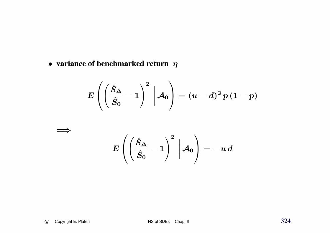
• variance of benchmarked return η
E
( S∆
S0
− 1
)2 ∣∣∣∣A0
= (u − d)2 p (1 − p)
=⇒
E
( S∆
S0
− 1
)2 ∣∣∣∣A0
= −ud
c⃝ Copyright E. Platen NS of SDEs Chap. 6 324

• binomial “volatility”
σ∆ =
√√√√√ 1
∆E
( S∆
S0
− 1
)2 ∣∣∣∣A0
=
√−ud
∆
• under the BS model option price increases for increasing volatility,
here not necessarily the case for European call price
SδH∆0 =
((1 + u) S0 − K
) (σ∆)2 ∆
u (u − d)
substantial freedomin u and d,not satisfactory do tosimplicity of the binomial model
c⃝ Copyright E. Platen NS of SDEs Chap. 6 325

Multi-Period Binomial Model
• benchmarked price of the stock
t = n∆
upwardSn∆ = S(n−1)∆ (1 + u)
probability
p =−d
u − d
c⃝ Copyright E. Platen NS of SDEs Chap. 6 326

downward
Sn∆ = S(n−1)∆ (1 + d)
probability 1 − p
for n ∈ 1, 2, . . .
c⃝ Copyright E. Platen NS of SDEs Chap. 6 327

• European call on S2∆
three values
Suu = (1 + u)2 S0
Sud = Sdu = (1 + u)(1 + d)S0
Sdd = (1 + d)2S0
binomial tree
c⃝ Copyright E. Platen NS of SDEs Chap. 6 328

• portfolioSδ2∆ = δ02∆ + δ12∆ S2∆
at time t = ∆
when S∆ = (1 + u) S0
SδH2∆
∆ =((1 + u)2 S0 − K
)+ −d
u − d+((1 + u)(1 + d) S0 − K
)+ u
u − d
for S∆ = (1 + d)S0
SδH2∆
∆ =((1 + u)(1 + d) S0 − K
)+ −d
u − d+((1 + d)2 S0 − K
)+ u
u − d
c⃝ Copyright E. Platen NS of SDEs Chap. 6 329

• fair benchmarked price at time t = 0
SδH2∆0 = p
(((1 + u)2 S0 − K
)+ −d
u − d
+((1 + u)(1 + d) S0 − K
)+ u
u − d
)
+(1 − p)
(((1 + u) (1 + d) S0 − K
)+ −d
u − d
+((1 + d)2 S0 − K
)+ u
u − d
)
perfect hedging strategy can be described
c⃝ Copyright E. Platen NS of SDEs Chap. 6 330

• binomial real world option pricing formula
similar to Cox, Ross & Rubinstein (1979) but real world pricing
SδHi∆0 = E
((Si∆ − K
)+ ∣∣∣A0
)
=i∑
k=0
i !
k ! (i − k) !pk (1 − p)i−k
×((1 + u)k(1 + d)i−k S0 − K
)+
c⃝ Copyright E. Platen NS of SDEs Chap. 6 331

= S0
i∑k=tk
i !
k ! (i − k) !pk (1 − p)i−k(1 + u)k(1 + d)i−k
− Ki∑
k=tk
i !
k ! (i − k) !pk (1 − p)i−k
tk first integer k for which (1 + u)k(1 + d)i−kS0 > K
(risk neutral pricing is here avoided)
c⃝ Copyright E. Platen NS of SDEs Chap. 6 332

• complementary binomial distribution
tN(tk, i, p) =
i∑k=tk
i !
k ! (i − k) !pk (1 − p)i−k
• binomial option pricing formula
SδHi∆0 = S0 tN(tk, i, 1−p) − K tN(tk, i, p)
similar to the Cox-Ross-Rubinstein binomial option pricing formula
similar to the Black-Scholes pricing formula
c⃝ Copyright E. Platen NS of SDEs Chap. 6 333

• hedging strategy
δk∆ = (δ0k∆, δ1k∆)⊤
self-financing benchmarked hedge portfolio
SδHi∆
k∆ = δ0(k−1)∆ + δ1(k−1)∆ Sk∆ = δ0k∆ + δ1k∆ Sk∆
c⃝ Copyright E. Platen NS of SDEs Chap. 6 334

• hedge ratio
δ1k∆ =
i−k∑ℓ=tkk
(i − k) !
ℓ ! (i − k − ℓ) !p(i−k−ℓ) (1 − p)ℓ
tkk smallest integer ℓ for which
(1 + u)ℓ (1 + d)i−k−ℓSk∆ > K
=⇒
δ0k∆ = SδHi∆
k∆ − δ1k∆ Sk∆
c⃝ Copyright E. Platen NS of SDEs Chap. 6 335

Approximating the Black-Scholes Price
step size ∆ → 0 limit
converges in a weak sense
• set u and d
ln(1 + u) = σ√∆
ln(1 + d) = −σ√∆
volatility parameter σ > 0
=⇒
c⃝ Copyright E. Platen NS of SDEs Chap. 6 336

u = expσ√∆− 1 ≈ σ
√∆
d = exp−σ
√∆− 1 ≈ −σ
√∆
for small ∆ ≪ 1 =⇒
σ∆ =1
√∆
√−ud ≈ σ
c⃝ Copyright E. Platen NS of SDEs Chap. 6 337

• stochastic processY ∆t = Sn∆
for t ∈ [n∆, (n + 1)∆), n ∈ 0, 1, . . .
Y ∆n∆+∆ = Y ∆
n∆ + Y ∆n∆ ηn
independent random variable ηn
P (ηn = u) = p =−d
u − d
P (ηn = d) = 1 − p =u
u − d
c⃝ Copyright E. Platen NS of SDEs Chap. 6 338

• rewrite approximately
Y ∆n∆+∆ ≈ Y ∆
n∆ + Y ∆n∆ σ
√∆ ξn
independent random variable ξn
P (ξn = 1) = p =1 − exp−σ
√∆
expσ√∆ − exp−σ
√∆
P (ξn = −1) = 1 − p
c⃝ Copyright E. Platen NS of SDEs Chap. 6 339

• by
E(Y ∆n∆+∆ − Y ∆
n∆
∣∣An∆
)= 0
E
((Y ∆n∆+∆ − Y ∆
n∆
)2 ∣∣∣An∆
)=
(Y ∆n∆
)2σ2∆ ∆
≈(Y ∆n∆
)2σ2 ∆
Y ∆ converges in a weak sense to
X = Xt, t ∈ [0, T ] as ∆ → 0, where
dXt = Xt σ dWt
=⇒
c⃝ Copyright E. Platen NS of SDEs Chap. 6 340

• for any suitable payoff function g
lim∆→0
E(g(Y ∆nT ∆
) ∣∣∣A0
)= E
(g(XT )
∣∣A0
)
c⃝ Copyright E. Platen NS of SDEs Chap. 6 341

=⇒
binomial option pricing formula
approximates for ∆ → 0
Black-Scholes pricing formula
S(δHT
)
0 = S0 N(d1) − K N(d2)
with
d1 =ln(S0
K) + 1
2σ2 T
σ√T
and
d2 = d1 − σ√T
c⃝ Copyright E. Platen NS of SDEs Chap. 6 342

Numerical Effects of Tree Methods
Option Prices from Binomial Trees
odd and even time steps
number at each time t = n∆
nodes starting with j = 1 from below
• binomial probability
pj(n) =n !
j ! (n − j) !pj (1 − p)n−j
for n ∈ 1, 2, . . . and j ∈ 1, 2, . . . , n with p ∈ (0, 1)
c⃝ Copyright E. Platen NS of SDEs Chap. 6 343

• European call or put option
setting at maturity the option value equal tothe European payoff
going one step back in time
obtain at each node the option value
expectation of the terminal payoff
using one step transition probabilities
c⃝ Copyright E. Platen NS of SDEs Chap. 6 344

at next step interpret obtained option price as new payoff
further step back in time
one step expectation
backward through the tree
at root of the tree
price of the option
• difference to Black-Scholes formulausing a CRR binomial tree
• CRR binomial tree
S0 = 1, K = 1, T = 1, r = 0.05, σ = 0.2
c⃝ Copyright E. Platen NS of SDEs Chap. 6 345

20 40 60 80 100nTimeSteps
0.0005
0.001
0.0015
0.002
0.0025
0.003
0.0035PriceError
Figure 6.1: Error of at-the-money European call option price for CRR bino-mial tree in dependence on the number of steps.
c⃝ Copyright E. Platen NS of SDEs Chap. 6 346

50 100 150 200 250nTimeSteps
0
0.0002
0.0004
0.0006
0.0008
0.001
0.0012PriceError
Figure 6.2: Error for out-of-the money CRR binomial European call in de-pendence on the number of time steps.
c⃝ Copyright E. Platen NS of SDEs Chap. 6 347

6 7 8 9 10
Log2nTimeSteps
-14
-12
-10
-8
-6Log2Error
Gamma
Delta
Price
Figure 6.3: Log-log plot of absolute weak error for at-the-money price, deltaand gamma of CRR binomial European call.
c⃝ Copyright E. Platen NS of SDEs Chap. 6 348

ln(µ(∆)) ≈ −3.91695 − 0.999291 ln
(T
∆
)
β ≈ 1.0
c⃝ Copyright E. Platen NS of SDEs Chap. 6 349

6 7 8 9 10
Log2nTimeSteps
-16
-14
-12
-10
-8
Log2Error
Gamma
Delta
Price
Figure 6.4: Log-log plot of absolute weak error for out-of-the money price,delta and gamma of CRR binomial European call.
c⃝ Copyright E. Platen NS of SDEs Chap. 6 350

6 7 8 9 10
Log2nTimeSteps
-20
-17.5
-15
-12.5
-10
-7.5
Log2Error
Gamma
Delta
Price
Figure 6.5: Log-log plot of the absolute error for in-the-money price, deltaand gamma of CRR binomial European call.
c⃝ Copyright E. Platen NS of SDEs Chap. 6 351

Binomial American Pricing
200 400 600 800 1000nTimeSteps
0.06075
0.060775
0.0608
0.060825
0.06085
0.060875
0.0609
AmericanPutPrice
Figure 6.6: CRR binomial American put prices.c⃝ Copyright E. Platen NS of SDEs Chap. 6 352

0 0.2 0.4 0.6 0.8 1Time
0.75
0.8
0.85
0.9
0.95
StockPrice
Figure 6.7: Early exercise boundary for American put.
c⃝ Copyright E. Platen NS of SDEs Chap. 6 353

Pricing on a Trinomial Tree
• next time step
S(d + 1), Sm or S(u + 1), d + 1 < m < u + 1
d = e−λσ√
∆ − 1
m = 1
u = eλσ√
∆ − 1
λ a free parameter
c⃝ Copyright E. Platen NS of SDEs Chap. 6 354

• Boyle (1988) trinomial probabilities
pd =(W − R) (u + 1)2 − (R − 1) (u + 1)3
u2 (u + 2)
pm = 1 − pd − pu
pu =(W − R) (u + 1) − (R − 1)
u2 (u + 2)
with
W = R2 eσ2∆
andR = er∆
for λ = 1 CRR binomial model
c⃝ Copyright E. Platen NS of SDEs Chap. 6 355

• first and second moment of the BS model are matched
pd (d + 1) + pm m + pu (u + 1) = R
and
pd (d+ 1)2 + pm m2 + pu (u+ 1)2 −R2 = e2r∆ (eσ2∆ − 1)
c⃝ Copyright E. Platen NS of SDEs Chap. 6 356

• Kamrad & Ritchken (1991) probabilities
pd =1
2λ2−
(r − σ2
2)√∆
2λσ
pm = 1 −1
λ2
pu =1
2λ2+
(r − σ2
2)√∆
2λσ
c⃝ Copyright E. Platen NS of SDEs Chap. 6 357

• matches the first and second moment of the logarithm
pd ln(d + 1) + pu ln(u + 1) =
(r −
σ2
2
)∆
pd (ln(d + 1))2 + pu (ln(u + 1))2 ≈ σ2∆ +
(r −
σ2
2
)2
∆2
applying Boyle’s trinomial tree with λ =√3
c⃝ Copyright E. Platen NS of SDEs Chap. 6 358

20 40 60 80 100nTimeSteps
0.001
0.002
0.003
0.004PriceError
Figure 6.8: Absolute error for Boyle’s trinomial at-the-money European call.
c⃝ Copyright E. Platen NS of SDEs Chap. 6 359

50 100 150 200 250nTimeSteps
0
0.00025
0.0005
0.00075
0.001
0.00125
0.0015PriceError
Figure 6.9: Absolute error for out-of-the money Boyle’s trinomial Europeancall with K = 1.1.
c⃝ Copyright E. Platen NS of SDEs Chap. 6 360

6 7 8 9 10
Log2nTimeSteps
-14
-12
-10
-8
-6Log2Error
Gamma
Delta
Price
Figure 6.10: Log-log plot of absolute error for at-the-money price, delta andgamma of Boyle’s trinomial European call.
c⃝ Copyright E. Platen NS of SDEs Chap. 6 361

6 7 8 9 10
Log2nTimeSteps
-16
-14
-12
-10
-8
-6
Log2Error
Gamma
Delta
Price
Figure 6.11: Log-log plot of absolute error for out-of-the money price, deltaand gamma of Boyle’s trinomial European call.
c⃝ Copyright E. Platen NS of SDEs Chap. 6 362

Black-Scholes Modification of a Tree
Broadie & Detemple (1997)
one step before maturity using Black-Scholes formula
=⇒
Black-Scholes modification of a tree
used to price American options
c⃝ Copyright E. Platen NS of SDEs Chap. 6 363

7 7.5 8 8.5 9 9.5 10
Log2nTimeSteps
-19
-18
-17
-16
-15
-14
-13
Log2Error
BBS
BTree
Figure 6.12: Log-log plot of absolute error with and without Black-Scholesmodification for CRR binomial out-of-the money European call.
c⃝ Copyright E. Platen NS of SDEs Chap. 6 364

Smooth Payoff
• cubic payoff
g(S) = S3 =
(S0 exp
(r −
σ2
2
)T + σWT
)3
• theoretical value
E(g(ST )) = (S0)3 exp(3 r + 4σ2) T
c⃝ Copyright E. Platen NS of SDEs Chap. 6 365
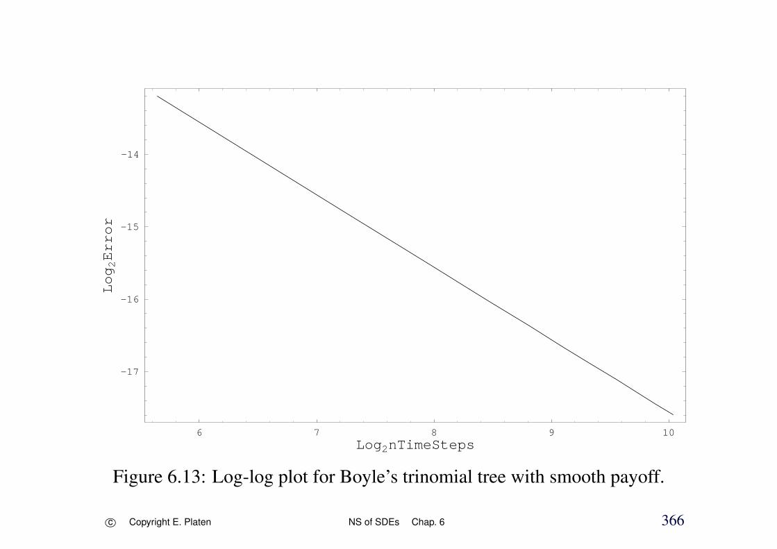
6 7 8 9 10Log2nTimeSteps
-17
-16
-15
-14
Log2Error
Figure 6.13: Log-log plot for Boyle’s trinomial tree with smooth payoff.
c⃝ Copyright E. Platen NS of SDEs Chap. 6 366

• Heston-Zhou trinomial tree
m = exp
(r −
σ2
2
)∆
d = m exp−σ
√3∆
− 1
u = m expσ√3∆
− 1
with probabilities
pd = pu =1
6
c⃝ Copyright E. Platen NS of SDEs Chap. 6 367

2 4 6 8 10Log2nTimeSteps
-30
-27.5
-25
-22.5
-20
-17.5
-15
Log2Error
Figure 6.14: Log-log plot for Heston-Zhou trinomial tree with smooth pay-off.
c⃝ Copyright E. Platen NS of SDEs Chap. 6 368
• calculating European calls
nonsmooth payoff experimentally only β ≈ 1.0
c⃝ Copyright E. Platen NS of SDEs Chap. 6 369
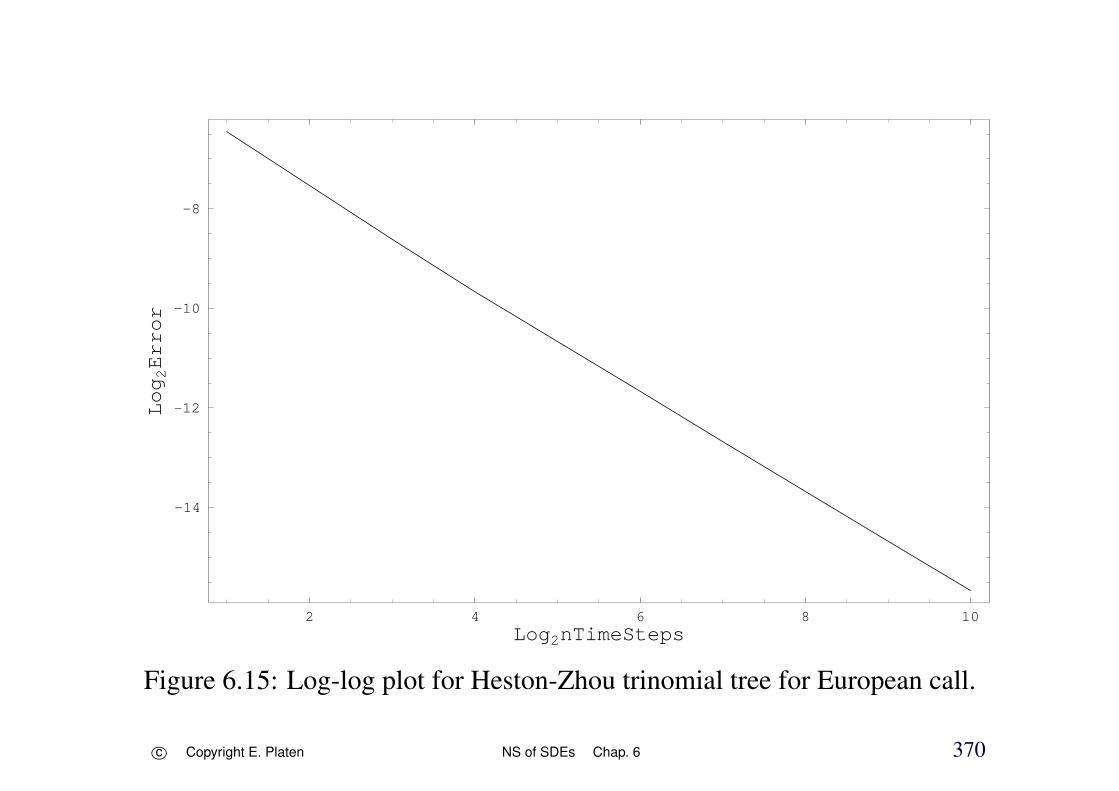
2 4 6 8 10Log2nTimeSteps
-14
-12
-10
-8
Log2Error
Figure 6.15: Log-log plot for Heston-Zhou trinomial tree for European call.
c⃝ Copyright E. Platen NS of SDEs Chap. 6 370

Extrapolation
• Richardson extrapolation
Kloeden & Pl. (1992b)
Glasserman (2004)
V ∆g,2(T ) = 2E
(g(Y ∆T
))− E
(g(Y 2∆T
))
if the leading error coefficients are appropriate
CRR binomial tree method
first weak order experimentally
c⃝ Copyright E. Platen NS of SDEs Chap. 6 371
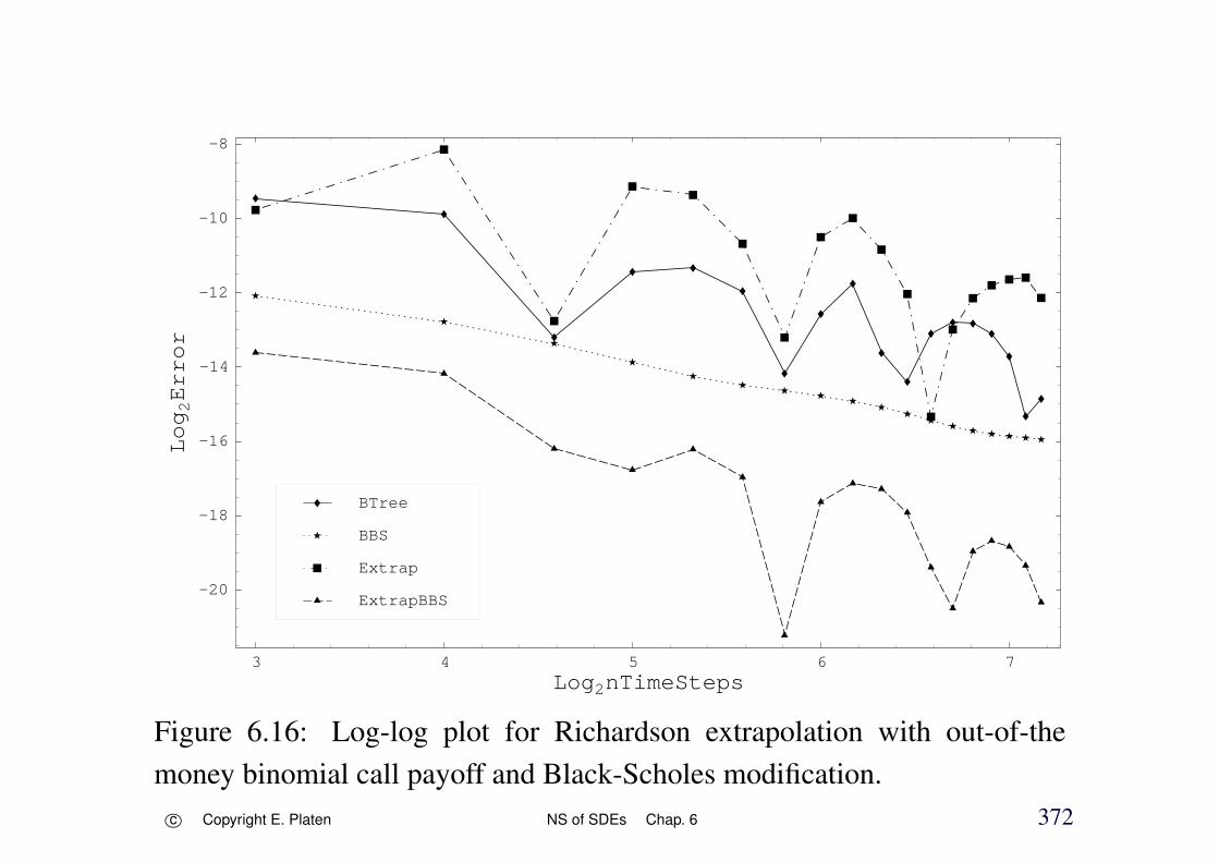
3 4 5 6 7
Log2nTimeSteps
-20
-18
-16
-14
-12
-10
-8
Log2Error
ExtrapBBS
Extrap
BBS
BTree
Figure 6.16: Log-log plot for Richardson extrapolation with out-of-themoney binomial call payoff and Black-Scholes modification.
c⃝ Copyright E. Platen NS of SDEs Chap. 6 372

• smooth payoffg(S) = S3
CRR binomial tree
Richardson extrapolation
c⃝ Copyright E. Platen NS of SDEs Chap. 6 373

1 2 3 4 5 6 7Log2nTimeSteps
-20
-18
-16
-14
-12
-10Log2Error
Figure 6.17: Log-log plot for Richardson extrapolation with CRR binomialtree for smooth payoff.
c⃝ Copyright E. Platen NS of SDEs Chap. 6 374

• extrapolation method
Heston & Zhou (2000)
V ∆g,4(T ) =
1
21
(32E
(g(Y ∆T
))−12E
(g(Y 2∆T
))+E
(g(Y 4∆T
)) )
c⃝ Copyright E. Platen NS of SDEs Chap. 6 375

2 2.5 3 3.5 4 4.5 5Log2nTimeSteps
-38
-36
-34
-32
-30
-28
-26Log2Error
Figure 6.18: Log-log plot for the absolute error of a fourth order extrapola-tion using the second order Heston-Zhou trinomial tree for smooth payoff.
c⃝ Copyright E. Platen NS of SDEs Chap. 6 376

• trinomial extrapolation for European call prices
2 3 4 5 6 7Log2nTimeSteps
-20
-18
-16
-14
-12
-10Log2Error
Figure 6.19: Log-log plot for a fourth order extrapolation for out-of-themoney Heston-Zhou trinomial European calls.
c⃝ Copyright E. Platen NS of SDEs Chap. 6 377
Efficiency of Simplified Schemes
Bruti-Liberati & Pl. (2004)
random bits generators
Weak Taylor Schemes and Simplified Methods
• SDEdXt = a(t,Xt) dt + b(t,Xt) dWt
• payoff function g(XT )
• equidistant time discretization τn = n∆, ∆ = TN
c⃝ Copyright E. Platen NS of SDEs Chap. 6 378

• simplified weak Euler scheme
Yn+1 = Yn + a(τn, Yn)∆ + b(τn, Yn)∆Wn
P (∆Wn = ±√∆) =
1
2
first three moments of ∆Wn match
E(∆Wn) = E(∆Wn) = 0
E((∆Wn)2) = E((∆Wn)
2) = ∆
E((∆Wn)3) = E((∆Wn)
3) = 0
c⃝ Copyright E. Platen NS of SDEs Chap. 6 379

• weak order 2.0 Taylor scheme
Yn+1 = Yn + a∆ + b∆Wn +1
2b′ b
(∆W 2
n
)− ∆
+
1
2
(a a′ +
1
2a′′b2
)∆2
+ a′ b∆Zn +
(a b′ +
1
2b′′b2
)∆Wn ∆ − ∆Zn
∆Zn =
∫ τn+1
τn
∫ z
τn
dWz ds
c⃝ Copyright E. Platen NS of SDEs Chap. 6 380

• simplified weak order 2.0 Taylor scheme
Yn+1 = Yn + a∆ + b∆Wn +1
2b b′
(∆Wn
)2− ∆
+1
2
(a a′ +
1
2a′′b2
)∆2
+1
2
(a′ b + a b′ +
1
2b′′b2
)∆Wn ∆
P(∆Wn = ±
√3∆)=
1
6, P
(∆Wn = 0
)=
2
3
first five moments are matchedβ = 3 or 4Kloeden & Pl. (1992b) and Hofmann (1994)
c⃝ Copyright E. Platen NS of SDEs Chap. 6 381

• numerical stability
• fully implicit weak Euler scheme
Yn+1 = Yn +
a (τn+1, Yn+1) − b (τn+1, Yn+1)
×∂
∂yb (τn+1, Yn+1)
∆
+ b (τn+1, Yn+1)∆Wn
Makes for certain diffusion coefficients no sense !
c⃝ Copyright E. Platen NS of SDEs Chap. 6 382

• simplified fully implicit Euler scheme
Yn+1 = Yn +
a (τn+1, Yn+1) − b (τn+1, Yn+1)
×∂
∂yb (τn+1, Yn+1)
∆
+ b (τn+1, Yn+1)∆Wn
β = 1.0
c⃝ Copyright E. Platen NS of SDEs Chap. 6 383

Random Bits Generators
• polar Marsaglia-Bray method
coupled with linear congruential random number generator
Press, Teukolsky, Vetterling & Flannery (2002)
pair of independent standard Gaussian random variables
• random bits generator
Bruti-Liberati & Pl. (2004)
generates a single bit 0 or 1 with probability 0.5
theory of primitive polynomials modulo 2
every primitive polynomial modulo 2 of order n defines a recurrence re-
c⃝ Copyright E. Platen NS of SDEs Chap. 6 384

lation for obtaining a new bit from the n preceding ones with maximallength
c⃝ Copyright E. Platen NS of SDEs Chap. 6 385

Numerical Results
• SDEdXt = µXt dt + σXt dWt
XT = X0 exp
(µ −
σ2
2
)T + σWT
A Smooth Payoff Function
• simplified methods achieve almost exactly the same accuracy of theirTaylor counterparts.
c⃝ Copyright E. Platen NS of SDEs Chap. 6 386

-8 -6 -4 -2 0Log2dt
-15
-12.5
-10
-7.5
-5
-2.5
0
2.5Log2WError
2Taylor
FImpEuler
Euler
Figure 6.20: Log-log plot of the weak error for the Euler, fully implicit Eulerand order 2.0 weak Taylor schemes.
c⃝ Copyright E. Platen NS of SDEs Chap. 6 387

0.5 1 1.5 2 2.5 3 3.5 4-Log2WError
-2
0
2
4
6
Log2CPU-Time
S2Taylor
SFimpEul
SEuler
2Taylor
FImpEul
Euler
Figure 6.21: Log-log plot of CPU time versus the weak error.
c⃝ Copyright E. Platen NS of SDEs Chap. 6 388
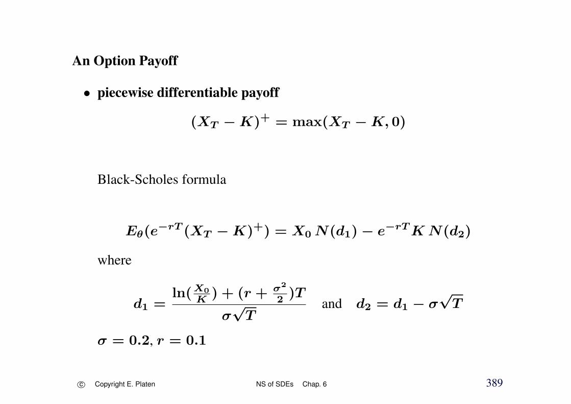
An Option Payoff
• piecewise differentiable payoff
(XT − K)+ = max(XT − K, 0)
Black-Scholes formula
Eθ(e−rT (XT − K)+) = X0 N(d1) − e−rTK N(d2)
where
d1 =ln(X0
K) + (r + σ2
2)T
σ√T
and d2 = d1 − σ√T
σ = 0.2, r = 0.1
c⃝ Copyright E. Platen NS of SDEs Chap. 6 389

-5 -4 -3 -2 -1 0Log2dt
-12
-11
-10
-9
-8
-7Log2WError
SEuler
Euler
Figure 6.22: Log-log plot of weak error for call option with Euler and sim-plified Euler scheme.
c⃝ Copyright E. Platen NS of SDEs Chap. 6 390

6.5 7 7.5 8 8.5 9 9.5 10-Log2WError
-4
-2
0
2
Log2CPU-Time
SEuler
Euler
Figure 6.23: Log-log plot of CPU time versus weak error for call option withEuler and simplified Euler scheme.
c⃝ Copyright E. Platen NS of SDEs Chap. 6 391
7 Partial Differential Equation Methods
PDEs and Diffusions
Second Order Parabolic Partial Differential Equations
financial market models
Markovian type
diffusion processes
or jump diffusion processes
c⃝ Copyright E. Platen BA to QF Chap. 7 392

• transition density
p(t, x; s, y)
Wiener process
• Kolmogorov backward equation
∂p(t, x; T, y)
∂t+
1
2
∂2p(t, x; T, y)
∂x2= 0
for t ∈ [0, T ] and x, y ∈ ℜ
c⃝ Copyright E. Platen BA to QF Chap. 7 393

• derivative price
expectation of a future payoff
integrable payoff g(WT )
u(t, x) = E(g(WT )
∣∣At
)=
∫ℜg(y) p(t, x; T, y) dy
when Wt = x
• only integrability of g(·) p(·) is required !
c⃝ Copyright E. Platen BA to QF Chap. 7 394

under integrability conditions on g ∂P∂t
and g ∂2P∂x2
=⇒∂u(t, x)
∂t=
∫ℜg(y)
∂p(t, x; T, y)
∂tdy
and
∂2u(t, x)
∂x2=
∫ℜg(y)
∂2p(t, x; T, y)
∂x2dy
for (t, x) ∈ (0, T ) × ℜ
=⇒
c⃝ Copyright E. Platen BA to QF Chap. 7 395

• Kolmogorov backward PDE
∂u(t, x)
∂t+
1
2
∂2u(t, x)
∂x2
=
∫ℜg(y)
(∂
∂t+
1
2
∂2
∂x2
)p(t, x; T, y) dy
= 0
for (t, x) ∈ (0, T ) × ℜ
c⃝ Copyright E. Platen BA to QF Chap. 7 396

Since p(T, x; T, y) = δ(y − x)
Dirac delta measure=⇒
• terminal condition
u(T, x) = g(x)
for x ∈ ℜ
c⃝ Copyright E. Platen BA to QF Chap. 7 397

• Feynman-Kac formula
pricing function
Kolmogorov backward equation
PDEs naturally arise in finance
rare explicit solution
=⇒ numerical methods
diffusion phenomenon is present in the price formation
=⇒ second order linear parabolic PDEs
heat equation
c⃝ Copyright E. Platen BA to QF Chap. 7 398

• linear PDE
if u1(t, x) and u2(t, x) are solutions
then so is
c1u1(t, x) + c2u2(t, x)
• second order PDE
highest order derivative occurring ∂2u(t,x)∂x2
c⃝ Copyright E. Platen BA to QF Chap. 7 399
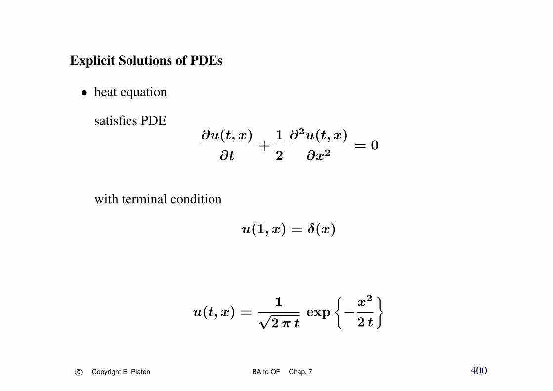
Explicit Solutions of PDEs
• heat equation
satisfies PDE∂u(t, x)
∂t+
1
2
∂2u(t, x)
∂x2= 0
with terminal condition
u(1, x) = δ(x)
u(t, x) =1
√2π t
exp
−
x2
2 t
c⃝ Copyright E. Platen BA to QF Chap. 7 400

• exploiting symmetry group methods
Craddock & Pl. (2004)
analytic formulas for transition densities
c⃝ Copyright E. Platen BA to QF Chap. 7 401

Generalized Square Root Processes
• SDEdXt = a(Xt) dt +
√2Xt dWt
• transition density
p(s, x; z, y) = p(t, x, y), t = z − s
∂p(t, x, y)
∂t= x
∂2p(t, x, y)
∂x2+ a(x)
∂p(t, x, y)
∂x
for t ∈ (0,∞) with
p(0, x, y) = δ(x − y)
for x, y ∈ (0,∞)
c⃝ Copyright E. Platen BA to QF Chap. 7 402

a(·) is a drift function
0.5 1 1.5 2 2.5 3x
0.5
1
1.5
2
2.5
3
3.5
Figure 7.1: Diffusion function of generalized square root process.
c⃝ Copyright E. Platen BA to QF Chap. 7 403

(i)a(x) = α > 0
squared Bessel process of dimension ν = 2α
dXt = αdt +√2Xt dWt
p(t, x, y) =1
t
(x
y
) 1−α2
Kα−1
(2√x y
t
)exp
−
(x + y)
t
Kr modified Bessel function of the first kind of order r
c⃝ Copyright E. Platen BA to QF Chap. 7 404

0.1
0.2
t
1
2
3
y
0
1
2
3
0
1
2
Figure 7.2: Transition density for case (i).
c⃝ Copyright E. Platen BA to QF Chap. 7 405

(ii)a(x) =
µx
1 + µ2x
for µ > 0
0.5 1 1.5 2 2.5 3x
0.2
0.4
0.6
0.8
1
1.2
Figure 7.3: Drift function of case (ii).
c⃝ Copyright E. Platen BA to QF Chap. 7 406

dXt =µXt
1 + µ2Xt
dt +√
2Xt dWt
p(t, x, y) =exp
− (x+y)
t
(1 + µ
2x)t
[(√x
y+
µ√x y
2
)K1
(2√x y
t
)+ t δ(y)
]
δ(·) Dirac delta function
for y = 0exp−x
t (1+µ
2 x)probability of absorbtion at zero
c⃝ Copyright E. Platen BA to QF Chap. 7 407

0.1
0.2
t
1
2
3
y
0
1
2
3
0
1
2
Figure 7.4: Transition density for case (ii).
c⃝ Copyright E. Platen BA to QF Chap. 7 408
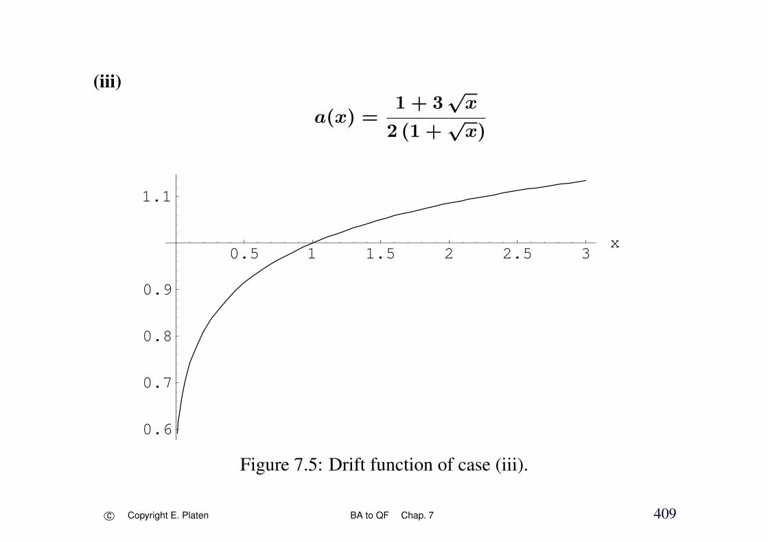
(iii)
a(x) =1 + 3
√x
2 (1 +√x)
0.5 1 1.5 2 2.5 3x
0.6
0.7
0.8
0.9
1.1
Figure 7.5: Drift function of case (iii).
c⃝ Copyright E. Platen BA to QF Chap. 7 409

dXt =1 + 3
√Xt
2 (1 +√Xt)
dt +√2Xt dWt
p(t, x, y) =cosh
(2√
x y
t
)√π y t (1 +
√x)
(1 +
√y tanh
(2√x y
t
))exp
−
(x + y)
t
c⃝ Copyright E. Platen BA to QF Chap. 7 410

0.1
0.2
t
1
2
3
y
0
1
2
3
0
1
2
Figure 7.6: Transition density for case (iii).
c⃝ Copyright E. Platen BA to QF Chap. 7 411

(iv)
a(x) = 1 + µ tanh
(µ +
1
2µ ln(x)
)for µ =
1
2
√5
2
0.5 1 1.5 2 2.5 3x
0.9
1.1
1.2
1.3
1.4
1.5
1.6
Figure 7.7: Drift function of case (iv).
c⃝ Copyright E. Platen BA to QF Chap. 7 412

dXt =
(1 + µ tanh
(µ +
1
2µ ln(Xt)
))dt +
√2Xt dWt
p(t, x, y) =
(x
y
)µ2[K−µ
(2√x y
t
)+ e2µ yµ Kµ
(2√x y
t
)]
×exp−x+y
t
(1 + exp2µxµ) t
c⃝ Copyright E. Platen BA to QF Chap. 7 413

0.1
0.2
t
1
2
3
y
0
1
2
3
0
1
2
Figure 7.8: Transition density for case (iv).
c⃝ Copyright E. Platen BA to QF Chap. 7 414

(v)
a(x) =1
2+
√x
0.5 1 1.5 2 2.5 3x
0.75
1.25
1.5
1.75
2
2.25
Figure 7.9: Drift function of case (v).
c⃝ Copyright E. Platen BA to QF Chap. 7 415

dXt =
(1
2+√
Xt
)dt +
√2Xt dWt
p(t, x, y) = cosh
((t + 2
√x)
√y
t
)exp−
√x
√π y t
exp
−
(x + y)
t−
t
4
c⃝ Copyright E. Platen BA to QF Chap. 7 416

0.1
0.2
t
1
2
3
y
0
1
2
3
0
1
2
Figure 7.10: Transition density for case (v).
c⃝ Copyright E. Platen BA to QF Chap. 7 417

(vi)
a(x) =1
2+
√x tanh(
√x)
0.5 1 1.5 2 2.5 3x
0.5
0.75
1.25
1.5
1.75
2
Figure 7.11: Drift function for case (vi).
c⃝ Copyright E. Platen BA to QF Chap. 7 418

dXt =
(1
2+√Xt tanh
(√Xt
))dt +
√2Xt dWt
p(t, x, y) =cosh
(2√
x y
t
)√π y t
cosh(√y)
cosh(√x)
exp
−
(x + y)
t−
t
4
c⃝ Copyright E. Platen BA to QF Chap. 7 419
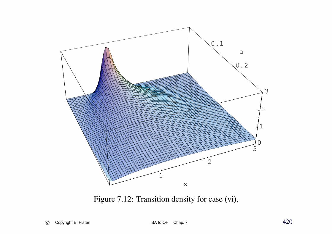
0.1
0.2
a
1
2
3
x
0
1
2
3
0
1
2
Figure 7.12: Transition density for case (vi).
c⃝ Copyright E. Platen BA to QF Chap. 7 420

(vii)
a(x) =1
2+
√x coth(
√x)
0.5 1 1.5 2 2.5 3x
1.6
1.8
2.2
Figure 7.13: Drift function for case (vii).
c⃝ Copyright E. Platen BA to QF Chap. 7 421
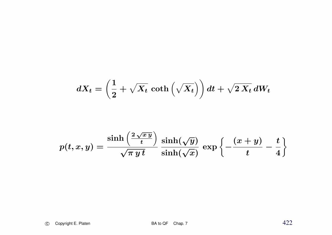
dXt =
(1
2+√Xt coth
(√Xt
))dt +
√2Xt dWt
p(t, x, y) =sinh
(2√
x y
t
)√π y t
sinh(√y)
sinh(√x)
exp
−
(x + y)
t−
t
4
c⃝ Copyright E. Platen BA to QF Chap. 7 422

0.1
0.2
a
1
2
3
x
0
1
2
3
0
1
2
Figure 7.14: Transition density for case (vii).
c⃝ Copyright E. Platen BA to QF Chap. 7 423

(viii)a(x) = 1 + cot(ln(
√x))
0.2 0.4 0.6 0.8x
-20
-10
10
Figure 7.15: Drift function for case (viii).
c⃝ Copyright E. Platen BA to QF Chap. 7 424

dXt =(1 + cot
(ln(√
Xt
)))dt +
√2Xt dt
p(t, x, y) =exp− (x+y)
t
2 ı t sin(ln(√x))
(y
ı2 Kı
(2√x y
t
)− y− ı
2 K−ı
(2√x y
t
))
c⃝ Copyright E. Platen BA to QF Chap. 7 425

0.1
0.2
a
0.20.4
0.60.8
1
x
0
1
2
3
4
0
1
2
3
Figure 7.16: Transition density for case (viii).
c⃝ Copyright E. Platen BA to QF Chap. 7 426

(ix)
a(x) = x coth
(x
2
)
0.5 1 1.5 2 2.5 3x
2.2
2.4
2.6
2.8
3
3.2
Figure 7.17: Drift function for case (ix).
c⃝ Copyright E. Platen BA to QF Chap. 7 427

dXt = Xt coth
(Xt
2
)dt +
√2Xt dWt
p(t, x, y) =sinh(y
2)
sinh(x2)exp
−
(x + y)
2 tanh( t2)
×[
exp t2
expt − 1
√x
yK1
( √x y
sinh( t2)
)+ δ(y)
]
c⃝ Copyright E. Platen BA to QF Chap. 7 428

0.1
0.2
a
1
2
3
x
0
1
2
3
0
1
2
Figure 7.18: Transition density for case (ix).
c⃝ Copyright E. Platen BA to QF Chap. 7 429

(x)
a(x) = x tanh
(x
2
)
0.5 1 1.5 2 2.5 3x
0.5
1
1.5
2
2.5
Figure 7.19: Drift function for case (x).
c⃝ Copyright E. Platen BA to QF Chap. 7 430

dXt = Xt tanh
(Xt
2
)dt +
√2Xt dWt
p(t, x, y) =cosh(y
2)
cosh(x2)exp
−
(x + y)
2 tanh( t2)
×[
exp t2
expt − 1
√x
yK1
( √x y
sinh( t2)
)+ δ(y)
]
c⃝ Copyright E. Platen BA to QF Chap. 7 431

0.1
0.2
a
1
2
3
x
0
1
2
3
0
1
2
Figure 7.20: Transition density for case (x).
c⃝ Copyright E. Platen BA to QF Chap. 7 432

Finite Difference Methods
Derivative Pricing Problem
numerical approximations
finite difference methods
Richtmeyer & Morton (1967)
Smith (1985)
Tavella & Randall (2000)
Shaw (1998)
Wilmott, Dewynne & Howison (1993)
c⃝ Copyright E. Platen BA to QF Chap. 7 433

• risk factor SDE
dXt = a(t,Xt) dt + b(t,Xt) dWt
for t ∈ [0, T ] with X0 > 0
• discounted payoff
u(T,XT ) = H(XT )
c⃝ Copyright E. Platen BA to QF Chap. 7 434
• discounted pricing function
u(·, ·)
PDE
∂u(t, x)
∂t+ a(t, x)
∂u(t, x)
∂x+
1
2(b(t, x))2
∂2u(t, x)
∂x2= 0
for t ∈ [0, T ] and x ∈ [0,∞)
terminal condition
u(T, x) = H(x)
c⃝ Copyright E. Platen BA to QF Chap. 7 435

Kolmogorov backward equation
Feynman-Kac formula
calculating conditional expectation
u(t,Xt) = E(H(XT )
∣∣At
)
can be also obtained as the fair benchmarked price
c⃝ Copyright E. Platen BA to QF Chap. 7 436

Spatial Differences
deterministic Taylor formula
∂u(t, x)
∂x=
u(t, x + ∆x) − u(t, x − ∆x)
2∆x+ R1(t, x)
∂2u(t, x)
∂x2=
u(t,x+∆x)−u(t,x)∆x
− (u(t,x)−u(t,x−∆x))∆x
2∆x+ R2(t, x)
=u(t, x + ∆x) − 2u(t, x) + u(t, x − ∆x)
2 (∆x)2
+R2(t, x)
c⃝ Copyright E. Platen BA to QF Chap. 7 437

• equally spaced grid
X 1∆x = xk = k∆x : k ∈ 0, 1, . . . , N
for N ∈ 2, 3, . . .
spatial discretization
xk+1 − xk = ∆x
writinguk(t) = u(t, xk)
c⃝ Copyright E. Platen BA to QF Chap. 7 438

=⇒∂u(t, xk)
∂x=
uk+1(t) − uk−1(t)
2∆x+ R1(t, xk)
∂2u(t, xk)
∂x2=
uk+1(t) − 2uk(t) + uk−1(t)
2 (∆x)2+ R2(t, xk)
for k ∈ 1, 2, . . . , N−1
c⃝ Copyright E. Platen BA to QF Chap. 7 439
• interior values uk(t) for k ∈ 1, 2, . . . , N−1
• boundary values u0(t) and uN(t)
• exampleu0(t) = 2u1(t) − u2(t)
and
uN(t) = 2uN−1(t) − uN−2(t)
c⃝ Copyright E. Platen BA to QF Chap. 7 440

• approximate system of ODEs
vectoru(t) = (u0(t), u1(t), . . . , uN(t))⊤
du(t)
dt−
A(t)
(∆x)2u(t) + R(t) = 0
R(t) remainder terms
• matrix
A(t) = [Ai,j(t)]Ni,j=0
c⃝ Copyright E. Platen BA to QF Chap. 7 441

A0,0(t) = A0,2(t) = AN,N−2(t) = AN,N(t) = (∆x)2
A0,1(t) = AN,N−1(t) = −2 (∆x)2
Ak,k(t) = −(b(t, xk))2
Ak,k−1(t) = −1
2(Ak,k(t) + a(t, xk)∆x)
Ak,k+1(t) = −1
2(Ak,k(t) − a(t, xk)∆x)
Ak,j(t) = 0
c⃝ Copyright E. Platen BA to QF Chap. 7 442

for k ∈ 1, 2, . . . , N−1 and |k − j| > 1
A =
(∆x)2 −2(∆x)2 (∆x)2 0 . . . 0 0 0
A1,0 A1,1 A1,2 0 . . . 0 0 0
0 A2,1 A2,2 A2,3 . . . 0 0 0
......
...... . . .
......
...
0 0 0 0 . . . AN−2,N−2 AN−2,N−1 0
0 0 0 0 . . . AN−1,N−2 AN−1,N−1 AN−1,N
0 0 0 0 . . . (∆x)2 −2(∆x)2 (∆x)2
c⃝ Copyright E. Platen BA to QF Chap. 7 443
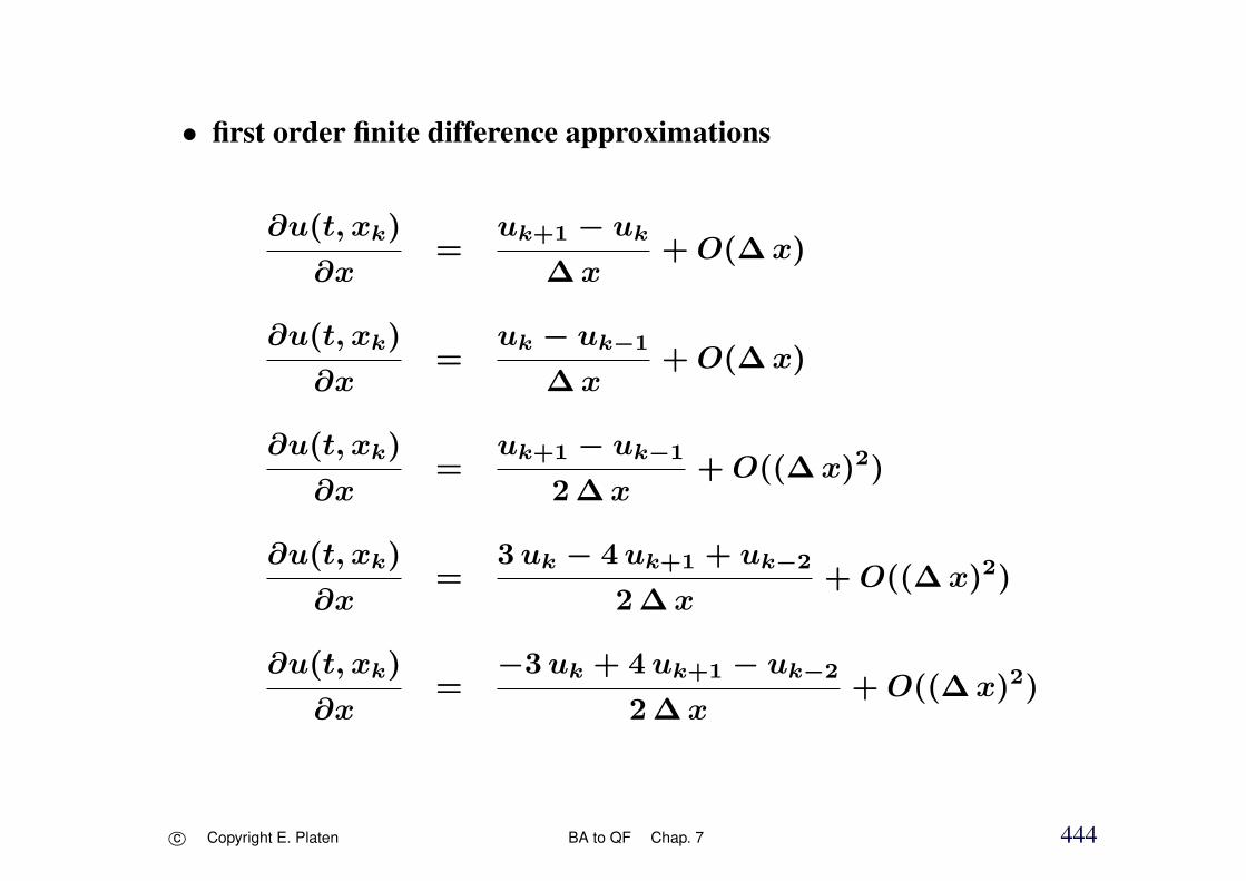
• first order finite difference approximations
∂u(t, xk)
∂x=
uk+1 − uk
∆x+ O(∆x)
∂u(t, xk)
∂x=
uk − uk−1
∆x+ O(∆x)
∂u(t, xk)
∂x=
uk+1 − uk−1
2∆x+ O((∆x)2)
∂u(t, xk)
∂x=
3uk − 4uk+1 + uk−2
2∆x+ O((∆x)2)
∂u(t, xk)
∂x=
−3uk + 4uk+1 − uk−2
2∆x+ O((∆x)2)
c⃝ Copyright E. Platen BA to QF Chap. 7 444

• second order spatial finite differences
∂2u(t, xk)
∂x2=
uk − 2uk−1 + uk−2
(∆x)2+ O(∆x)
∂2u(t, xk)
∂x2=
uk+2 − 2uk+1 + uk
(∆x)2+ O(∆x)
∂2u(t, xk)
∂x2=
uk+1 − 2uk + uk−1
(∆x)2+ O((∆x)2)
∂2u(t, xk)
∂x2=
2uk − 5uk−1 + 4uk−2 − uk−3
(∆x)2+ O((∆x)2)
∂2u(t, xk)
∂x2=
−uk+3 + 4uk+2 − 5uk+1 + 2uk
(∆x)2+ O((∆x)2)
c⃝ Copyright E. Platen BA to QF Chap. 7 445

Time Difference Approximation
=⇒
• approximate vector ODE
du(t) ≈A(t)
(∆x)2u(t) dt
for t ∈ (0, T ) with terminal condition
u(T ) = (H(x0), . . . ,H(xN))⊤
use discrete time approximations for ODEs
c⃝ Copyright E. Platen BA to QF Chap. 7 446

• time discretization τn = n∆, n ∈ 0, 1, . . . , nT
Euler scheme=⇒
u(τn+1) = u(τn) + A(τn)u(τn)∆
(∆x)2
for n ∈ 0, 1, . . . , nT , u(T ) = u(τnT )
=⇒uk(T ) = u(T, xk) = H(xk)
for all k ∈ 0, 1, . . . , N
constitutes a finite difference method
c⃝ Copyright E. Platen BA to QF Chap. 7 447

The Theta Method
family of implicit Euler schemes
• theta method
u(τn+1) = u(τn)+(θ A(τn+1)u(τn+1)+(1−θ)A(τn)u(τn)
) ∆
(∆x)2
degree of implicitness θ
θ = 0 =⇒ Euler or explicit method
interior of a circle
region of A-stability
c⃝ Copyright E. Platen BA to QF Chap. 7 448

θ = 1 =⇒
• fully implicit method
u(τn+1) = u(τn) + A(τn+1)u(τn+1)∆
(∆x)2
A-stable
unconditionally stable
c⃝ Copyright E. Platen BA to QF Chap. 7 449

θ = 12
=⇒
• Crank-Nicolson method
u(τn+1) = u(τn)+1
2
(A(τn+1)u(τn+1)+A(τn)u(τn)
) ∆
(∆x)2
deterministic trapezodial method
A-stable
unconditionally stable
certain stability issues
c⃝ Copyright E. Platen BA to QF Chap. 7 450

• solve at each time step a coupled system of equations
large, sparse linear system of equations
A(τn) = A
Crank-Nicolson method
u(τn+1) = u(τn) +1
2A(u(τn+1) + u(τn)
) ∆
(∆x)2
=⇒(I −
1
2A
∆
(∆x)2
)u(τn+1) =
(I +
1
2A
∆
(∆x)2
)u(τn)
c⃝ Copyright E. Platen BA to QF Chap. 7 451

With
M = I −1
2A
∆
(∆x)2
and
Bn =
(I +
1
2A
∆
(∆x)2
)u(τn)
rewrite linear system of equations
M u(τn+1) = Bn
needs to invert the matrix M
c⃝ Copyright E. Platen BA to QF Chap. 7 452

Sparse Matrix Solvers
• direct solver
tridiagonal solver known as Gaussian elimination method
• iterative solver
accuracy criterion
flexibility and efficiency
Barrett et al. (1994)
c⃝ Copyright E. Platen BA to QF Chap. 7 453

• Jacobi method
systemM u = B
M = [M i,j]Ni,j=1, u = (u1, . . . , uN)⊤ and B = (B1, . . . , BN)⊤
• kth iteration step
uik =
1
M i,i
Bi −∑j =i
M i,j ujk−1
uk = (u1k, . . . , u
Nk )⊤ kth iteration
c⃝ Copyright E. Platen BA to QF Chap. 7 454

• Gauss-Seidel method
uik =
1
M i,i
Bi −∑j<i
M i,j ujk −
∑j>i
M i,j ujk−1
improvements are worked in during the step
c⃝ Copyright E. Platen BA to QF Chap. 7 455
• successive over relaxation method
uik = α ui
k + (1 − α)uik−1
with
uik =
1
M i,i
Bi −∑j<i
M i,j ujk −
∑j>i
M i,j ujk−1
α ∈ ℜ
averaging a Gauss-Seidel iterate
c⃝ Copyright E. Platen BA to QF Chap. 7 456

Predictor-Corrector Methods
• modified trapezoidal method
corrector
u(τn+1) = u(τn)+1
2
(A(τn+1) u(τn+1)+A(τn)u(τn)
) ∆
(∆x)2
predictor
u(τn+1) = u(τn) + A(τn)u(τn)∆
(∆x)2
c⃝ Copyright E. Platen BA to QF Chap. 7 457

• predictor-corrector method
corrector
u(τn+1) = u(τn) + A(τn+1) u(τn+1)∆
(∆x)2
predictor
u(τn+1) = u(τn) + A(τn)u(τn)∆
(∆x)2
does not propagate errors severely
even if ∆(∆x)2
not extremely small
c⃝ Copyright E. Platen BA to QF Chap. 7 458

Boundary Conditions
limS→0
cT,K(t, S) = 0
limS→∞
cT,K(t, S) = S − K exp−r (T − t)
boundary conditions have to be translated
into finite difference method
c⃝ Copyright E. Platen BA to QF Chap. 7 459

finite intervalxmin = x0 < . . . < xN = xmax
xmin = x0 = 0 with
u0(t) = 0
xmax = xN < ∞ where
uN(t) ≈ xN − K exp−r (T − t)
c⃝ Copyright E. Platen BA to QF Chap. 7 460

Truncation at the Boundaries
Xt = ln(St)
dXt =
(r −
σ2
2
)dt + σ dWt
terminal payoff f(x) ≥ 0
c⃝ Copyright E. Platen BA to QF Chap. 7 461

PDE
L u(t, x) =1
2σ2 ∂2u(t, x)
∂x2+
(r −
σ2
2
)∂u(t, x)
∂x− r u(t, x) = 0
for (t, x) ∈ (0, T ) × ℜ with
u(T, x) = f(x)
for x ∈ ℜ
c⃝ Copyright E. Platen BA to QF Chap. 7 462

• approximating problem
area [0, T ] × (−ℓ, ℓ)
finite difference method
• Dirichlet conditions
u(t, ℓ) and u(t,−ℓ) given values
• Neumann conditions
∂u(t,ℓ)∂x
and ∂u(t,−ℓ)∂x
c⃝ Copyright E. Platen BA to QF Chap. 7 463

For simplicity
PDEL uℓ(t, x) = 0
for (t, x) ∈ (0, T ) × (−ℓ, ℓ)
with Dirichlet boundary conditions
uℓ(t,−ℓ) = uℓ(t) and uℓ(t, ℓ) = uℓ(t)
for t ∈ [0, T )
with terminal boundary conditions
uℓ(T, x) = f(x)
for x ∈ [−ℓ, ℓ]
c⃝ Copyright E. Platen BA to QF Chap. 7 464

assume European payoff function f(·) is bounded
Lamberton & Lapeyre (2007)
=⇒
Lemma 7.1 For (t, x) ∈ (0, T ) × ℜ one has the limit
limℓ→∞
uℓ(t, x) = u(t, x).
c⃝ Copyright E. Platen BA to QF Chap. 7 465

Convergence of Finite Difference Approximation
theta method
u∆(τn+1) = u∆(τn) +(θ A(τn+1)u
∆(τn+1)
+ (1 − θ)A(τn)u∆(τn)
) ∆
(∆x)2
u∆k (τn) = u∆(τn, xk)
linearly interpolate in time and space
c⃝ Copyright E. Platen BA to QF Chap. 7 466

Assuming uniform boundedness of u and ∂u∂x
Raviart & Thomas (1983)
=⇒
Lemma 7.2 For θ ∈ [0, 12) it follows as ∆ and ∆x tend to zero with
∆(∆x)2
→ 0 that
lim∆→0
u∆(t, x) = u(t, x).
when ∆x gets too small =⇒ unreliable
c⃝ Copyright E. Platen BA to QF Chap. 7 467

Lemma 7.3 For θ ∈ [12, 1] it follows as ∆ and ∆x tend to zero that
lim∆→0
u∆(t, x) = uℓ(t, x)
for (t, x) ∈ (0, T ) × (−ℓ, ℓ).
ratio ∆(∆x)2
does not need to go to zero
Crank-Nicolson method θ = 12
smallest θ
c⃝ Copyright E. Platen BA to QF Chap. 7 468

Numerical Results on Finite Difference Methods
Black-Scholes dynamics
dSt = St (r dt + σ dWt)
zero lowest grid point in S
Smax as upper level
c⃝ Copyright E. Platen BA to QF Chap. 7 469

at maturity payoff function
invert the resulting tridiagonal matrix
stability of the explicit theta method
variable
α =
(σ2 S2
(∆x)2+ r
)∆
less than one
Wilmott, Dewynne & Howison (1993)
error be not enhanced
c⃝ Copyright E. Platen BA to QF Chap. 7 470

0.6
0.8
1
1.2
1.4
alpha0.8
0.9
1
1.1
1.2
Stock Price
0
0.1
0.2
0.3
Call Price
0.6
0.8
1
1.2
1.4
alpha
Figure 7.21: Prices in dependence on α and S0 for the explicit finite differ-ence method.
c⃝ Copyright E. Platen BA to QF Chap. 7 471
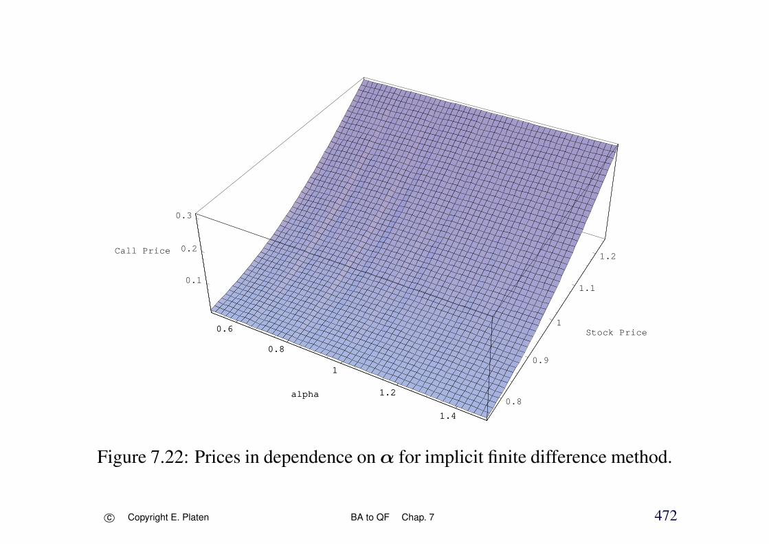
0.6
0.8
1
1.2
1.4
alpha0.8
0.9
1
1.1
1.2
Stock Price
0.1
0.2
0.3
Call Price
0.6
0.8
1
1.2
1.4
alpha
Figure 7.22: Prices in dependence on α for implicit finite difference method.
c⃝ Copyright E. Platen BA to QF Chap. 7 472

On the Accuracy of the Finite Difference Methods
for prices Crank-Nicolson scheme is always superior
symmetric averaging =⇒
higher order of convergence
four digit accuracy one more digit of precision
four digits of precision
five times more CPU time with explicit method
five digits Crank-Nicolson 20 times faster
c⃝ Copyright E. Platen BA to QF Chap. 7 473
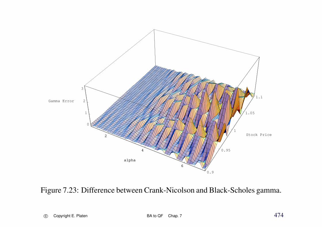
2
4
6
alpha
0.9
0.95
1
1.05
1.1
Stock Price
0
1
2
3
Gamma Error
2
4
6
alpha
Figure 7.23: Difference between Crank-Nicolson and Black-Scholes gamma.
c⃝ Copyright E. Platen BA to QF Chap. 7 474

2
4
6
alpha
0.9
0.95
1
1.05
1.1
Stock Price
0
0.1
0.2
0.3
0.4
Gamma Error
2
4
6
alpha
Figure 7.24: Difference between gamma from implicit method and Black-Scholes formula.
c⃝ Copyright E. Platen BA to QF Chap. 7 475

ReferencesBarrett, R., M. Berry, T. F. Chan, J. Demmel, J. Dongarra, V. Eijkhout, R. Pozo, C. Romine, & H. van der Vorst (1994). Templates for the Solution of
Linear Systems: Building Blocks for Iterative Methods. SIAM, Philadelphia.
Boyle, P. P. (1977). A Monte Carlo approach. J. Financial Economics 4, 323–338.
Boyle, P. P. (1988). A lattice framework for option pricing with two state variables. J. Financial and Quantitative Analysis 23, 1–12.
Boyle, P. P., M. Broadie, & P. Glasserman (1997). Monte Carlo methods for security pricing. Computational financial modelling. J. Econom. Dynam.Control 21(8-9), 1267–1321.
Bratley, P., B. L. Fox, & L. Schrage (1987). A Guide to Simulation (2nd ed.). Springer.
Broadie, M. & J. Detemple (1997). The valuation of American options on multiple assets. Math. Finance 7(3), 241–286.
Broadie, M. & P. Glasserman (1997). Pricing American - style securities using simulation. Computational financial modelling. J. Econom. Dynam.Control 21(8-9), 1323–1352.
Bruti-Liberati, N. & E. Pl. (2004). On the efficiency of simplified weak Taylor schemes for Monte Carlo simulation in finance. In ComputationalScience - ICCS 2004, Volume 3039 of Lecture Notes in Comput. Sci., pp. 771–778. Springer.
Burrage, P. M. (1998). Runge-Kutta methods for stochastic differential equations. Ph. D. thesis, University of Queensland, Brisbane, Australia.
Chang, C. C. (1987). Numerical solution of stochastic differential equations with constant diffusion coefficients. Math. Comp. 49, 523–542.
Clewlow, L. & A. Carverhill (1992). Efficient Monte Carlo valuation and hedging of contingent claims. Technical report, Financial Options ResearchCenter, University of Warwick. 92/30.
Clewlow, L. & A. Carverhill (1994). Quicker on the curves. Risk 7(5).
Cox, J. C., S. A. Ross, & M. Rubinstein (1979). Option pricing: A simplified approach. J. Financial Economics 7, 229–263.
Craddock, M. & E. Pl. (2004). Symmetry group methods for fundamental solutions. J. of Differential Equations 207(2), 285–302.
Ermakov, S. M. (1975). Die Monte Carlo-Methode und verwandte Fragen. Hochschulbucher fur Mathematik, Band 72. VEB Deutscher Verlag derWissenschaften, Berlin. (in German) Translated from Russian by E. Schincke and M. Schleiff.
Ermakov, S. M. & G. A. Mikhailov (1982). Statistical Modeling (2nd ed.). Nauka, Moscow.
Fishman, G. S. (1996). Monte Carlo: Concepts, Algorithms and Applications. Springer Ser. Oper. Res. Springer.
c⃝ Copyright E. Platen References 476

Fournie, E., J. M. Lasry, & N. Touzi (1997). Monte Carlo methods for stochastic volatility models. In Numerical Methods in Finance, pp. 146–164.Cambridge Univ. Press, Cambridge.
Fu, M. C. (1995). Pricing of financial derivatives via simulation. In C. Alexopoulus, K. Kang, W. Lilegdon, and D. Goldsman (Eds.), Proceedings ofthe 1995 Winter Simulation Conference. Piscataway, New Jersey: Institute of Electrical and Electronics Engineers.
Glasserman, P. (2004). Monte Carlo Methods in Financial Engineering, Volume 53 of Appl. Math. Springer.
Goldman, D., D. Heath, G. Kentwell, & E. Pl. (1995). Valuation of multi-factor interest rate dependent contingent claims. In E. Platen (Ed.), Workshopon Stochastic and Finance, pp. 153–170. Australian National University, Canberra. FMRR 004-95.
Grant, D., D. Vora, & D. Weeks (1997). Path-dependent options: Extending the Monte Carlo simulation approach. Management Science 43(11),1589–1602.
Hammersley, J. M. & D. C. Handscomb (1964). Monte Carlo Methods. Methuen, London.
Heath, D. (1995). Valuation of derivative securities using stochastic analytic and numerical methods. Ph. D. thesis, ANU, Canberra.
Heath, D. & E. Pl. (2002). A variance reduction technique based on integral representations. Quant. Finance 2(5), 362–369.
Hernandez, D. B. & R. Spigler (1992). A-stability of implicit Runge-Kutta methods for systems with additive noise. BIT 32, 620–633.
Hernandez, D. B. & R. Spigler (1993). Convergence and stability of implicit Runge-Kutta methods for systems with multiplicative noise. BIT 33,654–669.
Heston, S. L. & G. Zhou (2000). On the rate of convergence of discrete-time contingent claims. Math. Finance 10(1), 53–75.
Higham, D. J. (2000). Mean-square and asymptotic stability of numerical methods for stochastic ordinary differential equations. SIAM J. Numer.Anal. 38, 753–769.
Hofmann, N. (1994). Beitrage zur schwachen Approximation stochastischer Differentialgleichungen. Ph. D. thesis, Dissertation A, Humboldt Uni-versitat Berlin.
Hofmann, N. & E. Pl. (1994). Stability of weak numerical schemes for stochastic differential equations. Comput. Math. Appl. 28(10-12), 45–57.
Hofmann, N. & E. Pl. (1996). Stability of superimplicit numerical methods for stochastic differential equations. Fields Inst. Commun. 9, 93–104.
Hofmann, N., E. Pl., & M. Schweizer (1992). Option pricing under incompleteness and stochastic volatility. Math. Finance 2(3), 153–187.
Joy, C., P. P. Boyle, & K. S. Tan (1996). Quasi Monte Carlo methods in numerical finance. Management Science 42(6), 926–938.
Kalos, M. H. & P. A. Whitlock (1986). Monte Carlo Methods. Vol. I. Basics. Wiley, New York.
Kamrad, B. & P. Ritchken (1991). Multinomial approximating models for options with k state variables. Management Science 37, 1640–1652.
c⃝ Copyright E. Platen References 477

Kloeden, P. E. & E. Pl. (1992a). Higher order implicit strong numerical schemes for stochastic differential equations. J. Statist. Phys. 66(1/2),283–314.
Kloeden, P. E. & E. Pl. (1992b). Numerical Solution of Stochastic Differential Equations, Volume 23 of Appl. Math. Springer. Third printing, (firstedition (1992)).
Kloeden, P. E., E. Pl., & H. Schurz (2003). Numerical Solution of SDEs Through Computer Experiments. Universitext. Springer. Third correctedprinting, (first edition (1994)).
Lamberton, D. & B. Lapeyre (2007). Introduction to Stochastic Calculus Applied to Finance (2nd ed.). Chapman & Hall, London. Translation fromFrench.
Law, A. M. & W. D. Kelton (1991). Simulation Modeling and Analysis (2nd ed.). McGraw-Hill, New York.
Longstaff, F. A. & E. S. Schwartz (2001). Valuing American options by simulations: A simple least-squares approach. Rev. Financial Studies 14(1),113–147.
Maltz, F. H. & D. L. Hitzl (1979). Variance reduction in Monte-Carlo computations using multi-dimensional Hermite polynomials. J. Comput.Phys. 32, 345–376.
Maruyama, G. (1955). Continuous Markov processes and stochastic equations. Rend. Circ. Mat. Palermo 4, 48–90.
Milstein, G. N. (1974). Approximate integration of stochastic differential equations. Theory Probab. Appl. 19, 557–562.
Milstein, G. N. (1988). Numerical Integration of Stochastic Differential Equations. Urals Univ. Press, Sverdlovsk. (in Russian).
Milstein, G. N. (1995). Numerical Integration of Stochastic Differential Equations. Mathematics and Its Applications. Kluwer.
Milstein, G. N., E. Pl., & H. Schurz (1998). Balanced implicit methods for stiff stochastic systems. SIAM J. Numer. Anal. 35(3), 1010–1019.
Newton, N. J. (1994). Variance reduction for simulated diffusions. SIAM J. Appl. Math. 54(6), 1780–1805.
Pl., E. (1982). A generalized Taylor formula for solutions of stochastic differential equations. SANKHYA A 44(2), 163–172.
Pl., E. (1984). Beitrage zur zeitdiskreten Approximation von Itoprozessen. Habilitation, Academy of Sciences, Berlin.
Pl., E. (1995). On weak implicit and predictor-corrector methods. Math. Comput. Simulation 38, 69–76.
Pl., E. & L. Shi (2008). On the numerical stability of simulation methods for SDEs. Technical report, University of Technology, Sydney. QFRCResearch Paper 234.
Pl., E. & W. Wagner (1982). On a Taylor formula for a class of Ito processes. Probab. Math. Statist. 3(1), 37–51.
Press, W. H., S. A. Teukolsky, W. T. Vetterling, & B. P. Flannery (2002). Numerical Recipes in C++. The Art of Scientific Computing (2nd ed.).Cambridge University Press.
c⃝ Copyright E. Platen References 478

Raviart, P. A. & J. M. Thomas (1983). Introduction to the Numerical Analysis of Partial Differential Equations. Collection of Applied Mathematicsfor the Master’s Degree. Masson, Paris. (in French).
Richtmeyer, R. & K. Morton (1967). Difference Methods for Initial-Value Problems. Interscience, New York.
Ripley, B. D. (1983). Stochastic Simulation. Wiley, New York.
Ross, S. M. (1990). A Course in Simulation. Macmillan.
Rubinstein, R. Y. (1981). Simulation and the Monte Carlo Method. Wiley Ser. Probab. Math. Statist. Wiley, New York.
Saito, Y. & T. Mitsui (1993a). Simulation of stochastic differential equations. Ann. Inst. Statist. Math. 45, 419–432.
Saito, Y. & T. Mitsui (1993b). T-stability of numerical schemes for stochastic differential equations. World Sci. Ser. Appl. Anal. 2, 333–344.
Saito, Y. & T. Mitsui (1996). Stability analysis of numerical schemes for stochastic differential equations. SIAM J. Numer. Anal. 33(6), 2254–2267.
Shaw, W. (1998). Pricing Derivatives with Mathematica. Cambridge University Press.
Smith, G. D. (1985). Numerical Solution of Partial Differential Equations: Finite Difference Methods (3rd ed.). Clarendon Press, Oxford.
Talay, D. & L. Tubaro (1990). Expansion of the global error for numerical schemes solving stochastic differential equations. Stochastic Anal.Appl. 8(4), 483–509.
Tavella, D. & C. Randall (2000). Pricing Financial Instruments. The Finite Difference Method. Wiley, New York.
Wagner, W. (1987). Unbiased Monte-Carlo evaluation of functionals of solutions of stochastic differential equations variance reduction and numericalexamples. Preprint P-Math-30/87 Inst. Math. Akad. der Wiss. der DDR.
Wagner, W. & E. Pl. (1978). Approximation of Ito integral equations. Preprint ZIMM, Akad. Wissenschaften, DDR, Berlin.
Wilmott, P., J. Dewynne, & S. Howison (1993). Option Pricing: Mathematical Models and Computation. Oxford Financial Press.
c⃝ Copyright E. Platen References 479