numerical methods in scientific computationjinbo/courses/numericalmethods_fall...exactly how will...

Numerical Methods in Scientific Computation

Lecture 2 Programming and SoftwareIntroduction to error analysis

Numerical Methods, Fall 2011 Lecture 2 1 Prof. Jinbo Bi

CSE, UConn

Packages vs. Programming• Packages

• MATLAB• Excel• Mathematica• Maple

• Packages do the work for you• Most offer an interactive environment


CSE, UConn

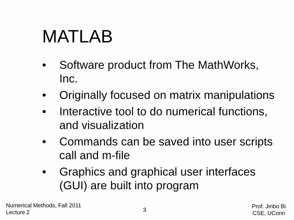
MATLAB• Software product from The MathWorks,

Inc.• Originally focused on matrix manipulations• Interactive tool to do numerical functions,

and visualization• Commands can be saved into user scripts

call and m-file• Graphics and graphical user interfaces

(GUI) are built into programNumerical Methods, Fall 2011 Lecture 2 3 Prof. Jinbo Bi

CSE, UConn

MATLAB• Base product is extended with a variety of

“toolboxes”• Optimization• Statistics• Curve fitting• Image processing


CSE, UConn

MATLAB• Example: Find roots of>> p = [1 -6 -72 -27]>> r = roots (p)>> r =

12.1229-5.7345-0.3884

27726 23 −−− xxx


CSE, UConn

• Advantages:• Large library of functions to evaluate a wide

variety of numerical problems• Interactive tool allows immediate evaluation

of results• Disadvantages

• Expensive• Not as fast as C/C++/FORTRAN code

MATLAB


CSE, UConn

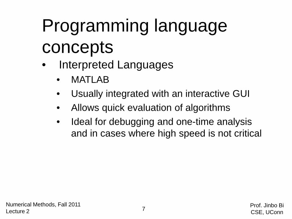
Programming language concepts• Interpreted Languages

• MATLAB• Usually integrated with an interactive GUI• Allows quick evaluation of algorithms• Ideal for debugging and one-time analysis

and in cases where high speed is not critical


CSE, UConn

Programming language concepts• Compiled Languages

• FORTRAN, C, C++• Source code is created with an editor as a plain text

file• Programs then needs to be “compiled” (converted

from source code to machine instructions with relative addresses and undefined external routines still needed).

• The compiled routines (called object modules) need then to be linked with system libraries.

• Faster execution than interpreted languages


CSE, UConn

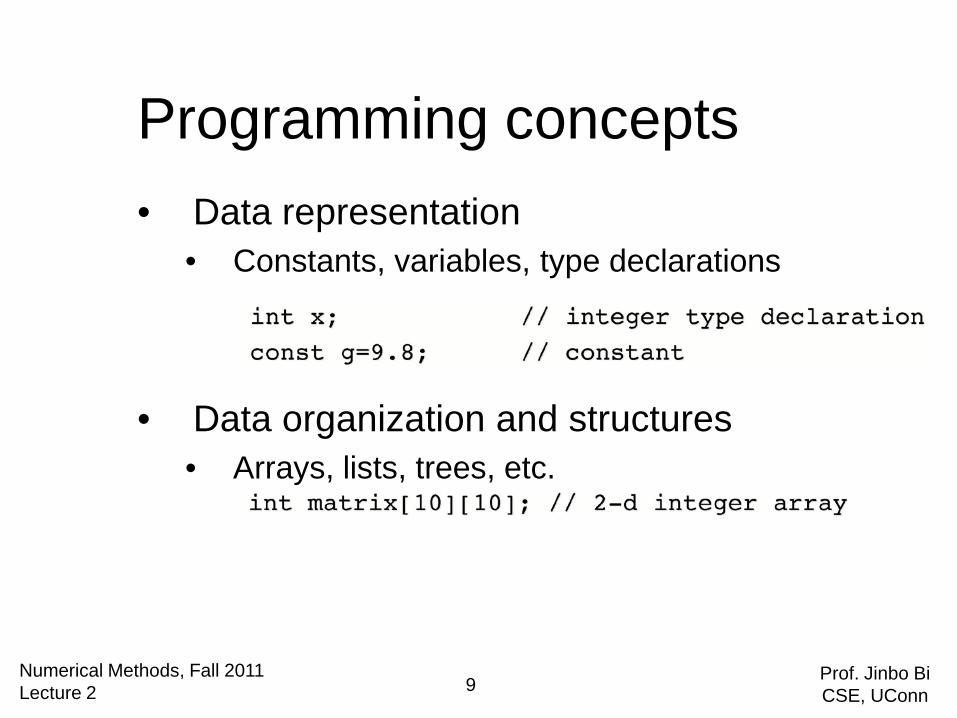
• Data representation• Constants, variables, type declarations

• Data organization and structures• Arrays, lists, trees, etc.

Programming concepts


CSE, UConn

• Mathematical formulas• Assignment, priority rules

• Input/Output• Stdin / Stdout, files, GUI



CSE, UConn

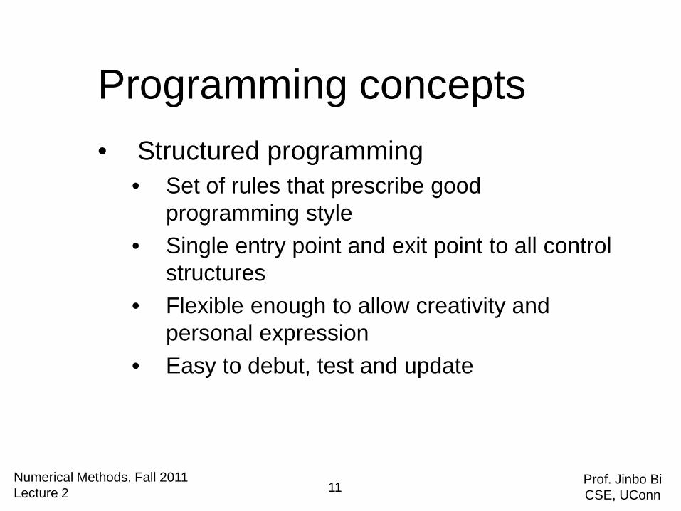
• Structured programming• Set of rules that prescribe good

programming style• Single entry point and exit point to all control

structures• Flexible enough to allow creativity and

personal expression• Easy to debut, test and update



CSE, UConn

• Control structures• Sequence• Selection• Repetition

• Computer code is clearer and easier to follow

Structured programming


CSE, UConn

• Flowcharts• Visual representation• Useful in planning

• Pseudocode• Simple representation of an algorithm• Basic program constructs without being

language-specific• Easy to modify and share with others

Algorithm expression


CSE, UConn

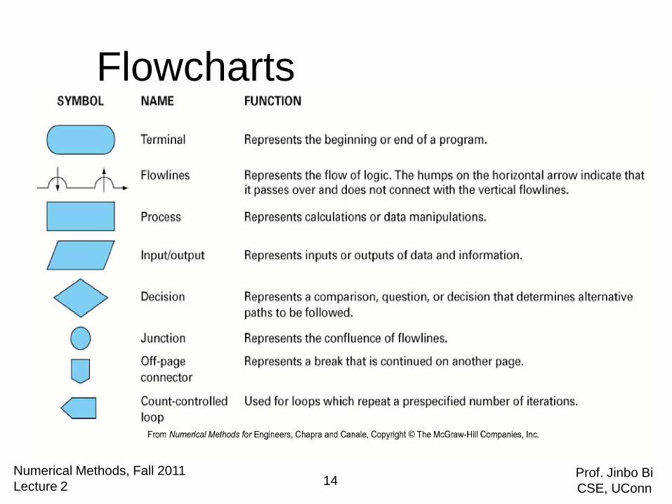
Flowcharts


CSE, UConn

• Sequence• Implement one

instruction at a time

Control structures


CSE, UConn

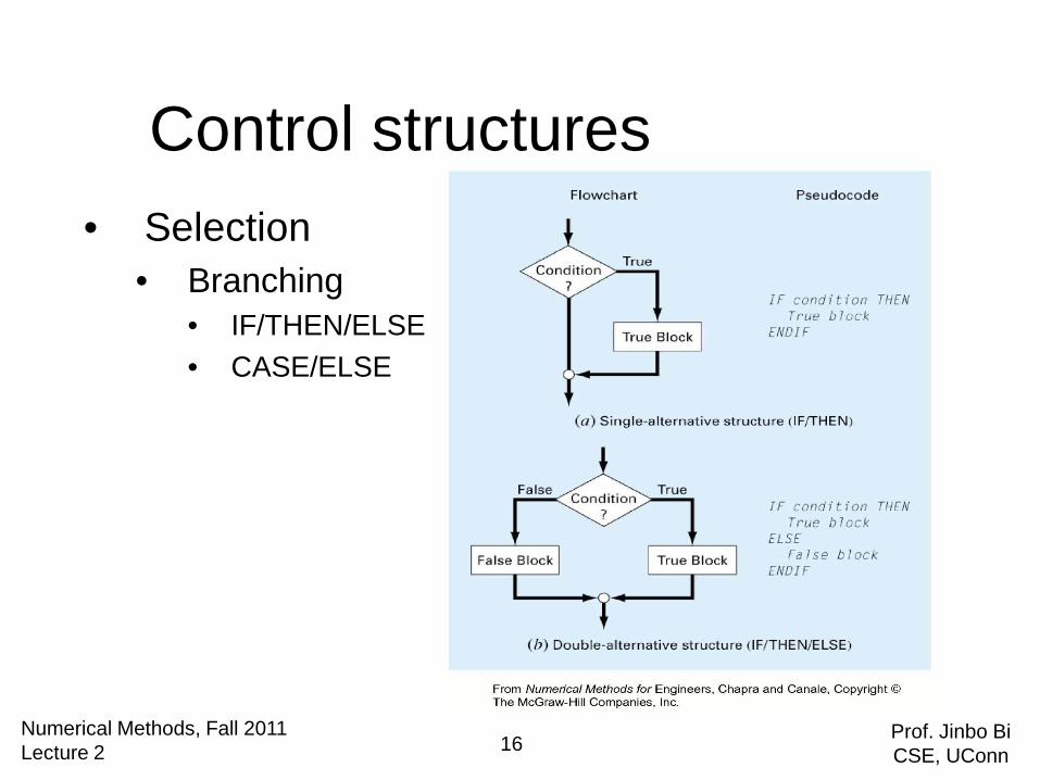
• Selection• Branching

• IF/THEN/ELSE• CASE/ELSE

Control structures


CSE, UConn

Control structures


CSE, UConn

• Repetition• DOEXIT loops (break loop)

• Similar to C while loop

• DOFOR loop (count-controlled)

Control structures


CSE, UConn

Control structures• pretest• posttest• midtest


CSE, UConn

Control structures


CSE, UConn

• Break complicated tasks into manageable parts

• Independent and self-contained• Well-defined modules with a single entry

point and single exit point• Always a good idea to return a value for

status or error code

Modular programming


CSE, UConn

• Makes logic easier to understand and digest

• Allows black-box development of modules

• Requires well-defined interfaces with no side effects

• Isolates errors• Allows for reuse of modules and

development of libraries

Modular programming


CSE, UConn

• Specification: A clear statement of the problem, the requirements, and any special parameters of operation

• Algorithm/Design: A flow chart or pseudo code representation of how exactly how will the problem be solved.

Software engineering approach


CSE, UConn

• Implementation: Breaking the algorithm into manageable pieces that can be coded into the language of choice, and putting all the pieces together to solve the problem.

• Verification: Checking that the implementation solves the original specification. In numerical problems, this is difficult because most of the time you don’t know what the correct answer is.

Software engineering approach


CSE, UConn

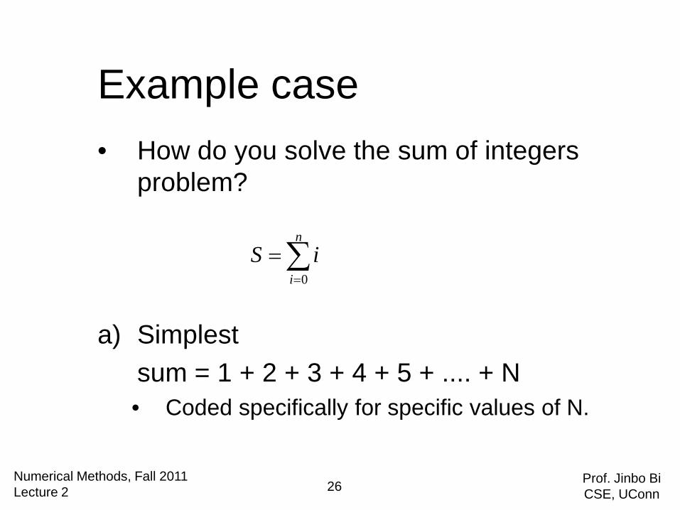
• How do you solve the sum of integers problem?

a) Simplestsum = 1 + 2 + 3 + 4 + 5 + .... + N• Coded specifically for specific values of N.

Example case

∑=

=n

iiS

0


CSE, UConn

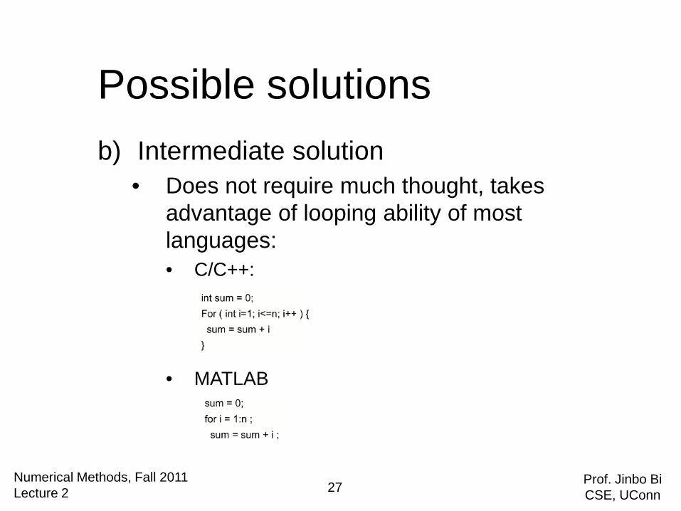
b) Intermediate solution• Does not require much thought, takes

advantage of looping ability of most languages:• C/C++:

• MATLAB

Possible solutions


CSE, UConn

c) Analytical solution• Requires some thought about the sequence

remember back to one of your math classes.

Possible solutions

2)1(* +

=nnsum


CSE, UConn

• What can fail in the above algorithms. (To know all the possible failure modes requires knowledge of how computers work). Some examples of failures are:

• For (b): This algorithm is fairly robust. • But, when N is large execution will be slow

compared to (c)

Verification of algorithm


CSE, UConn

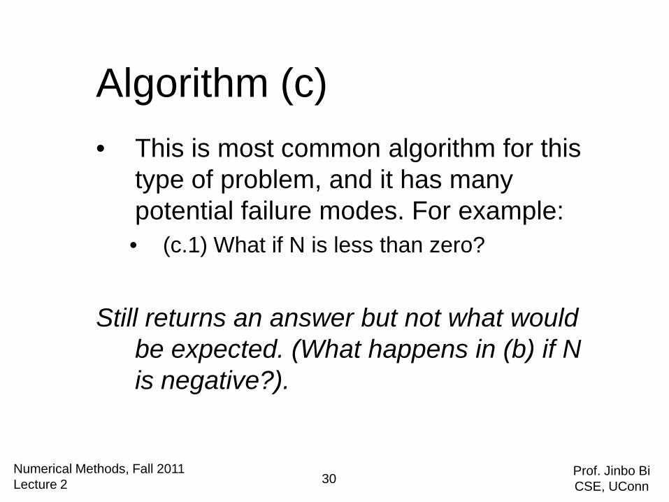
Algorithm (c)• This is most common algorithm for this

type of problem, and it has many potential failure modes. For example:• (c.1) What if N is less than zero?

Still returns an answer but not what would be expected. (What happens in (b) if N is negative?).


CSE, UConn

Algorithm (c)• (c.2) In which order will the multiplication

and division be done.For all values of N, either N or N+1 will be even

and therefore N*(N+1) will always be even but what if the division is done first? Algorithm will work half of the time.

If division is done first and N+1 is odd, the algorithm will return a result but it will not be correct. This is a bug. For verification, it means the algorithm works sometimes but not always.


CSE, UConn

Algorithm (c)• (c.3) What if N is very large?What is the maximum value N*(N+1) can

have?There are maximum values that integers can be represented in a computer and we may overflow. What happens then? Can we code this to handle large values of N?


CSE, UConn

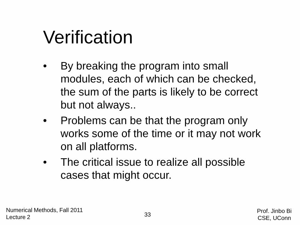
Verification• By breaking the program into small

modules, each of which can be checked, the sum of the parts is likely to be correct but not always..

• Problems can be that the program only works some of the time or it may not work on all platforms.

• The critical issue to realize all possible cases that might occur.


CSE, UConn

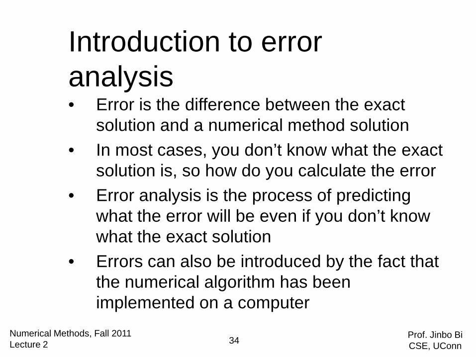
Introduction to error analysis• Error is the difference between the exact

solution and a numerical method solution• In most cases, you don’t know what the exact

solution is, so how do you calculate the error• Error analysis is the process of predicting

what the error will be even if you don’t know what the exact solution

• Errors can also be introduced by the fact that the numerical algorithm has been implemented on a computer


CSE, UConn

Significant digits• Can a number be used with confidence?• How accurate is the number?• How many digits of the number do we

trust?


CSE, UConn

Significant digits• Can the speed be estimated to

one decimal place?


CSE, UConn

• The significant digits of a number are those that can be used with confidence• The digits that are known with certainty plus

one estimated digit• zeros are not always significant digits

– 0.0001845, 0.001845, 0.01845– 4.53x104, 4.530x104, 4.5300x104

• Exact numbers vs. measured numbers• Exact numbers have an infinite number of

significant digits• π is an exact number but usually subject to

round-off

Significant digits


CSE, UConn

Significant digits


CSE, UConn

Accuracy and precision• Accuracy is how close a computed or

measured value is to the true value• Precision is how close individual computed

or measured values agree with each other• Reproducibility

• Inaccuracy/Bias vs. Imprecision/Uncertainty• Inaccuracy: systematic deviation from the truth• imprecision: magnitude of the scatter


CSE, UConn

Accuracy and precision


CSE, UConn

• The level of accuracy and precision required depend on the problem

• Error to represent both the inaccuracy and imprecision of predictions

Accuracy and precision


CSE, UConn

• Two general types of errors• Truncation errors – due to approximations of

exact mathematical functions• Round-off errors – due to limited significant

digit representation of exact numbers

Et = true value – approximation

Error definitions


CSE, UConn

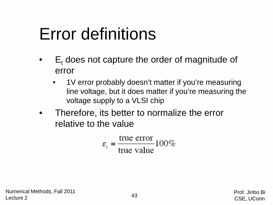
• Et does not capture the order of magnitude of error

• 1V error probably doesn’t matter if you’re measuring line voltage, but it does matter if you’re measuring the voltage supply to a VLSI chip

• Therefore, its better to normalize the error relative to the value

Error definitions


CSE, UConn

• Example:• Line voltage

• Chip supply voltage

Error definitions


CSE, UConn

• What if we don’t know the true value?• Use an approximation of the true value

• How do we calculate the approximate error?

• Use an iterative approach• Approximate error = current approximation –

previous approximation• Assumes that the iteration will converge

Error definitions

a


CSE, UConn

• For most problems, we are interested in keeping the error less than specified error tolerance

• How many iterations do you do, before you’re satisfied that the result is correct to at least n significant digits?

Error Definitions


CSE, UConn

• Infinite series expansion of ex

• As we add terms to the expansion, the expression becomes more exact

• Using this series expansion, can we calculate e0.5 to three significant digits?

Example


CSE, UConn

• Calculate the error tolerance

• First approximation

• Second approximation

• Error approximation

Example


CSE, UConn

• Third approximation

• Error approximation

Example


CSE, UConn

Example


CSE, UConn

Next class• HW1, due 9/8

• Chapra & Canale 6th Edition• 1.8 (typo: dy/dx -> dy/dt), 1.12, 2.5 (choose order

n=6), 2.14

• Next class• Continue on error analysis


CSE, UConn

numerical methods in scientific computationjinbo/courses/numericalmethods_fall...exactly how will...

Documents