Wayne State University

Wayne State University Dissertations

1-1-2011

Numerical methods for problems arising in riskmanagement and insuranceZhuo JinWayne State University,

Follow this and additional works at: http://digitalcommons.wayne.edu/oa_dissertations

Part of the Mathematics Commons

This Open Access Dissertation is brought to you for free and open access by DigitalCommons@WayneState. It has been accepted for inclusion inWayne State University Dissertations by an authorized administrator of DigitalCommons@WayneState.

Recommended CitationJin, Zhuo, "Numerical methods for problems arising in risk management and insurance" (2011). Wayne State University Dissertations.Paper 281.

NUMERICAL METHODS FOR PROBLEMS ARISING IN

RISK MANAGEMENT AND INSURANCE

by

ZHUO JIN

DISSERTATION

Submitted to the Graduate School

of Wayne State University,

Detroit, Michigan

in partial fulfillment of the requirements

for the degree of

DOCTOR OF PHILOSOPHY

2011

MAJOR: MATHEMATICS

Approved by:

———————————————————–Advisor Date

———————————————————–

———————————————————–

———————————————————–

DEDICATION

To my parents

ii

ACKNOWLEDGEMENTS

It is my great pleasure to thank those who provided me numerous supports for the

completion of the dissertation. In particular, I would like to express my sincerest appreciation

and deepest gratitude to my advisor, professor George Yin, for standing beside me during my

graduate study. His endless care, consistent support, inspiring guidance, valuable suggestions

enabled me to develop a comprehensive understanding of the stochastic control and actuarial

science. Furthermore, I benefited a lot from his distinct and elegant personality during the

five-year pursuit of my PhD degree.

I am taking this opportunity to thank Professor Paul Chow, Professor Tze Chien Sun,

and Professor Stephen Spurr for serving on my committee.

I owe a great debt of gratitude to Professor Hailiang Yang, who have provided timely

suggestions and support in both research and career. I am also grateful to Professor Shigeng

Hu, who helped me a lot when I studied in China.

I owe my thanks to Ms. Mary Klamo, Ms. Patricia Bonesteel, Professor Choon-Jai

Rhee, Professor John Breckenridge, Mr. James Veneri, Ms. Tiana Fluker, Professor Rafail

Khasminskii, Professor Alex Korostelev, Dr. Qingshuo Song, Dr. Chao Zhu, Dr. Shaobai

Kan, Dr. Son Luu Nguyen, and Mr. Lizhen Qin for their help and encouragement in one

way or another.

I would like to thank my parents for their unconditional and unlimited love and support.

My special gratitude goes to my wife for her love, encouragement, and sharing with me

everything.

Finally, but not least, I would like to express my appreciation to the entire Department

iii

of Mathematics for the hospitality and services. I enjoyed the warm and friendly atmosphere

in the department, and I appreciated the support I received during my study at Wayne State

University.

iv

TABLE OF CONTENTS

Dedication . . . . . . . . . . . . . . . . . . . . . . . . . . . . . . . . . . . . . . . . . . . . . . . . . . . . . . . . . . . . . . . . . . . . . . . . . . . . . . ii

Acknowledgements . . . . . . . . . . . . . . . . . . . . . . . . . . . . . . . . . . . . . . . . . . . . . . . . . . . . . . . . . . . . . . . . . . . . . iii

1 Introduction . . . . . . . . . . . . . . . . . . . . . . . . . . . . . . . . . . . . . . . . . . . . . . . . . . . . . . . . . . . . . . . . . . . . . .1

2 Optimal Annuity-Purchasing Strategies . . . . . . . . . . . . . . . . . . . . . . . . . . . . . . . . . . . . . . . 4

2.1 Formulation . . . . . . . . . . . . . . . . . . . . . . . . . . . . . . . . . . . . . . . . . . . . . . . . . . . . . . . . . . . . . . . . . . . 5

2.2 Constant Hazard Rate . . . . . . . . . . . . . . . . . . . . . . . . . . . . . . . . . . . . . . . . . . . . . . . . . . . . . . . . 10

2.2.1 Approximating Markov Chain . . . . . . . . . . . . . . . . . . . . . . . . . . . . . . . . . . . . . . . . 11

2.2.2 Main Results . . . . . . . . . . . . . . . . . . . . . . . . . . . . . . . . . . . . . . . . . . . . . . . . . . . . . . . . .20

2.3 General Hazard Rate . . . . . . . . . . . . . . . . . . . . . . . . . . . . . . . . . . . . . . . . . . . . . . . . . . . . . . . . . 28

2.3.1 Approximating Markov Chain . . . . . . . . . . . . . . . . . . . . . . . . . . . . . . . . . . . . . . . . 28

2.3.2 Main Results . . . . . . . . . . . . . . . . . . . . . . . . . . . . . . . . . . . . . . . . . . . . . . . . . . . . . . . . .31

2.4 Examples . . . . . . . . . . . . . . . . . . . . . . . . . . . . . . . . . . . . . . . . . . . . . . . . . . . . . . . . . . . . . . . . . . . . 41

2.4.1 Constant Hazard Rate . . . . . . . . . . . . . . . . . . . . . . . . . . . . . . . . . . . . . . . . . . . . . . . 41

2.4.2 General Hazard Rate . . . . . . . . . . . . . . . . . . . . . . . . . . . . . . . . . . . . . . . . . . . . . . . . .42

3 Dividend Optimization . . . . . . . . . . . . . . . . . . . . . . . . . . . . . . . . . . . . . . . . . . . . . . . . . . . . . . . . . 46

3.1 Formulation . . . . . . . . . . . . . . . . . . . . . . . . . . . . . . . . . . . . . . . . . . . . . . . . . . . . . . . . . . . . . . . . . .47

3.2 Numerical Algorithm . . . . . . . . . . . . . . . . . . . . . . . . . . . . . . . . . . . . . . . . . . . . . . . . . . . . . . . . .53

3.3 Convergence of Numerical Approximation . . . . . . . . . . . . . . . . . . . . . . . . . . . . . . . . . . . . 60

3.3.1 Local Consistency . . . . . . . . . . . . . . . . . . . . . . . . . . . . . . . . . . . . . . . . . . . . . . . . . . . . 61

v

3.3.2 Interpolations of Approximation Sequences . . . . . . . . . . . . . . . . . . . . . . . . . . . 62

3.3.3 Convergence of Surplus Processes . . . . . . . . . . . . . . . . . . . . . . . . . . . . . . . . . . . . 65

3.3.4 Convergence of Reward and Value Functions . . . . . . . . . . . . . . . . . . . . . . . . . 69

3.4 Numerical Example . . . . . . . . . . . . . . . . . . . . . . . . . . . . . . . . . . . . . . . . . . . . . . . . . . . . . . . . . . . 71

4 Further Remarks . . . . . . . . . . . . . . . . . . . . . . . . . . . . . . . . . . . . . . . . . . . . . . . . . . . . . . . . . . . . . . . 77

References . . . . . . . . . . . . . . . . . . . . . . . . . . . . . . . . . . . . . . . . . . . . . . . . . . . . . . . . . . . . . . . . . . . . . . . . . . . . . .79

Abstract . . . . . . . . . . . . . . . . . . . . . . . . . . . . . . . . . . . . . . . . . . . . . . . . . . . . . . . . . . . . . . . . . . . . . . . . . . . . . . . 83

Autobiographical Statement . . . . . . . . . . . . . . . . . . . . . . . . . . . . . . . . . . . . . . . . . . . . . . . . . . . . . . . . . . . . 85

vi

1

1 Introduction

This dissertation focuses on numerical methods for stochastic optimization problems aris-

ing in risk management and insurance. Both analytic properties and numerical results are

presented for several insurance models.

Due to the recent economic crisis, more and more people are concerned with their future

after retirement. According to the Transamerica Center for Retirement Studies, the number

of U.S. workers who are confident in their ability to retire comfortably has declined signif-

icantly in the past year. Thus, to better manage retirement has become an urgent issue.

One of the problems faced by numerous retirees is to find an optimal annuity-purchasing

strategy to minimize the probability that the individual outlives his or her wealth termed

the probability of lifetime ruin. Assuming the retiree maintains a pre-specified (exogenous)

consumption level, one aims to determine the optimal investment strategy, as well as the

optimal time to annuitize to minimize the probability that wealth will reach zero while the

individual is still alive.

Taking up the retirement management issue, in the first part of the dissertation, we focus

on the problem of investing in a risky financial market and purchasing annuities to minimize

the probability of lifetime ruin. We consider a regime-switching diffusion model, which in-

cludes both continuous dynamics and discrete events. The modulating stochastic process is

assumed to be a continuous-time Markov chain representing the random environment and

other random factors not included in the usual diffusion formulation. For example, the rate

of return and the volatility, and the insurance charge are modulated by a finite-state Markov

chain α(·), which represents the market modes and other economic conditions. For example,

2

when α(t) ∈ 1, 2, we use 1 to represent the bullish (up-trend) market and 2 the bearish

(down-trend) market. In general, M = 1, 2, . . . ,m for some positive integer m. As is

widely recognized, this regime-switching model appears to be more versatile and more real-

istic than the previous literature. The retirement management problem can be formulated

as a stochastic control problem. The solution of the resulting stochastic control problem

rests upon the solution of the associated systems of Hamilton-Jacobi-Bellman (HJB) equa-

tions and/or variational inequalities. Because of regime switching and the nonlinearity, it is

virtually impossible to obtain closed-form or analytic solutions for our problems. Thus we

are seeking viable alternative. In reference to the powerful methods of Markov chain approx-

imation initiated by Kushner and developed more extensively in Kushner and Dupuis [13],

we aim to find a good approximation to the underlying problems. By good approximation,

we mean that the numerical methods should be consistent with the systems of interests and

should converge to the right value.

In the second part of the dissertation, we consider dividend policy for regime-switching

compound Poisson models. In the literature, De Finetti suggested that a company would

seek to maximize the expectation of the present value of all dividends before possible ruin

and showed the optimal dividend-payment strategy is a barrier strategy in 1957, see [4].

Since then a host of researchers tried to address this optimality question under more general

and more realistic model assumptions. Nowadays, dividend optimization becomes a rich and

challenging field of research, which needs the combination of tools from analysis, probability,

and stochastic control. Similar to many papers in the literature, our objective is to maximize

the expected discounted total dividends until ruin. We model the surplus process using a

jump diffusion with regime-switching process. The process describing the regime switching

3

is assumed to be a continuous-time Markov chain representing the random environment.

As mentioned above, this model appears to be more versatile and more realistic than the

classical compound Poisson and diffusion models. However, to solve the problem under this

model, we need to solve a system of Hamilton-Jaccobi-Bellman (HJB) partial differential

equations instead of a single HJB equation. Solving the associated system of HJB equations

is a difficult task. Analytic solutions can not be obtained. A viable alternative is to construct

feasible numerical approximation schemes for finding a good approximation to the underlying

problems. Using the Markov chain approximation methods in [13] and in reference to the

numerical methods developed for general regime-switching jump diffusions in [18], we develop

an approximation procedure. The main ingredient is that we approximate the optimal

dividend payout strategy by a controlled Markov chain. To prove the convergence, we use

the methods of weak convergence. In addition to proving the convergence, we also provide

numerical results for demonstration. Note that in the actual computation, we can simply

use the well-known value or policy iteration techniques.

The rest of the dissertation is arranged as follows. Chapter 2 discusses Markov chain ap-

proximation for annuity-purchasing decision making to minimize the probability of financial

ruin for regime-switching wealth models. Chapter 3 focuses on optimal dividend policy for

regime-switching jump-diffusion model. A few further remarks are made in Chapter 4.

4

2 Optimal Annuity-Purchasing Strategies

To secure the post-retirement life, purchasing annuities from insurance companies is of crucial

importance. The recipient of the annuity could receive a continuous fixed payment through-

out the life. This life steam income could guarantee the retiree a given level of consumption.

On the other hand, since the Swedish actuary Filip Lundberg [14] introduced the classical

compound-Poisson risk model in 1903, probability of ruin is among the prime quantities to

measure the insurance risk. Therefore, to measure the financial risk of purchasing annuity

and managing portfolio becomes a big issue, that is what we are interested in.

A fruitful of results related to annuity were achieved in economics literature. Yaari [21]

proved that in the absence of bequest motives and in a deterministic financial economy con-

sumers will annuitize all of their liquid wealth. This result is generalized to a stochastic

environment by Richard in [16], and recently T. Davidoff and Diamond demonstrated the

robustness of Yaaris result in [6]. Similarly, Kapur and Orszag [12] and Brown [3] provide

theoretical and empirical guidance on the optimal time to annuitize under various market

structures. Optimal investment strategy to minimize the probability of lifetime ruin is con-

sidered by Young in [25], and Milevsky, Moore, and Young provide the annuity-purchasing

strategies to minimize the probability of lifetime ruin in [15]. The so-called regime-switching

models can be found in [7, 26, 27]; see also the related work [10, 22]. A comprehensive

treatment of switching diffusions can be found in [23].

Unlike the previous work, the wealth is modeled as a regime-switching diffusion modulat-

ed by a continuous-time Markov chain. Based on Markov chain approximation techniques,

an approximation procedure to find optimal annuity-purchasing strategies for minimizing

5

the probability of lifetime ruin is constructed. Several interesting results are obtained that

are consistent with the economics intuition.

2.1 Formulation

We use a controlled hybrid switching diffusion to represent the wealth. For simplicity, assume

the system to be one dimensional. Let (Ω,F , P ) be the probability space and Ft be a

filtration defined on it. Suppose that the discrete events take values in a finite set M =

1, . . . ,m and that α(·) is a continuous-time Markov chain having state space M and

generator Q = (qij). Let ω(·) be a standard Ft-Wiener process, and u(·) be an Ft-adapted

control, taking value in a compact set U . Such controls are said to be admissible.

Now we set up the optimal annuity-purchasing and investment problem for an individual

who seeks to minimize the probability that she or he outlives her or his wealth. The wealth

of the individual consists of investment incomes from the riskless asset, the risky assets, and

the income from the annuity after the purchase. To maintain a constant consumption rate,

the individual manages the portfolio to avoid the financial ruin before she or he dies.

Initial income could include social security benefits and defined benefit pension benefits.

We assume that the income variation only comes from buying life annuities by using money

from current wealth. We assume that with α(s) = i, the interest rate at time s is given by

r(i), and the individual can invest in a riskless asset with the yield rate r(i) and a risky asset

6

with the price H(s, i) at time s such thatdH(s, α(s)) = µ(s, α(s))H(s, α(s))ds+ σ(s, α(s))H(s, α(s))dω,

H(t, α(t)) = H0 > 0.

(2.1)

where µ(s, i) > r(i) and σ(s, i) > 0 for all i ∈ M. We use λ(t) to denote the hazard rate at

age t and λ(t) to denote the particular hazard rate function used to price the annuity. The

actuarial present value of perpetuity with the life stream payment of 1 dollar per year by

the interest rate r(α(t)) and the hazard rate λ with the discount is

a(t) =

∫ ∞

0

exp(−r(α(t))s) exp(−∫ t+s

t

λ(v)dv)ds

=∑i∈M

Iα(t)=i

∫ ∞

0

exp(−r(i)s) exp(−∫ t+s

t

λ(v)dv)ds,

(2.2)

where IA is the indicator function of the set A.

For each i ∈ M, c(i) denotes a constant rate that the individual consumes, W (s, i)

denotes the wealth of the individual at time s, and A(s, i) denotes a nonnegative income

rate at time s of after any annuity purchases at that time. Let u(s) be the amount that the

7

decision maker invests in the risky asset at time s, and 0 ≤ u ≤ W . The dynamic system is

dW (s, α(s)) = (r(α(s))W (s, α(s)) + (µ(s, α(s))− r(α(s))u(s)

−c(α(s)) + A(s, α(s)))ds+ σ(s, α(s))u(s)dω − a(s)dA(s, α(s)),

W (t, α(t)) = w ≥ 0,

A(t, α(t)) = A ≥ 0.

(2.3)

To simplify the dynamic system, we define the excess consumption Z(s, i) = c(i)−A(s, i)

with Z(s, i) being the net income the decision maker inquires with i ∈ M. Then the dynamic

system (2.3) can be rewritten as

dW (s, α(s)) = (r(α(s))W (s, α(s)) + (µ(s, α(s))− r(α(s))u(s)− Z(s, α(s)))ds

+σ(s, α(s))u(s)dω + a(s)dZ(s),

W (t, α(t)) = w ≥ 0,

Z(t, α(t)) = z ≥ 0,

(2.4)

Since if w ≥ za(t), the individual can purchase the annuity immediately to guarantee

a net income of z to avoid the lifetime ruin. Let τ0 be the time when the wealth reaches

zero and τd be the random time of death of the individual. With α(t) = i, denote the cost

8

function by

EIτ0<τd|W (t,i)=w, Z(t,i)=z, τ0>t,τd>t = P [τ0 < τd|W (t, i) = w, Z(t, i) = z, τ0 > t, τd > t]

= φ(w, z, t, i, u), i ∈ M.

(2.5)

Then, the probability of lifetime ruin ψ at time t (with α(t) = i)) can be represented on the

domain D = (w, z, t, i) : 0 ≤ w ≤ za(t), z ≥ 0, t ≥ 0, i ∈ M as

ψ(w, z, t, i) = infu,Z

φ(w, z, t, i, u), i ∈ M. (2.6)

Then ψ(w, z, t, α(t)) = 0 when w ≥ za(t). Note that τ0 = τ0(w, z, u). That is, it depends

on (w, z) as well on the control u. However, for notational simplicity, in what follows, we

suppress the (w, z, u) dependence.

Note that this problem is a combination of the continuous control (the investment strat-

egy u) and the singular control (the excess consumption Z). Combining stochastic control

techniques used in Milevsky, Moore, and Young (2006), and methods for treating regime-

switching diffusions in Yin and Zhu (2010), we can derive the Hamilton-Jacobi-Bellman

variational inequality, which is given in Proposition 2.1. Furthermore, the Hamilton-Jacobi-

Bellman equation with boundary conditions are presented in Proposition 2.2 and Proposi-

tion 2.3. The detailed derivations are omitted for brevity.

Proposition 2.1. The probability of lifetime ruin is a constrained viscosity solution of the

9

system of Hamilton-Jacobi-Bellman variational inequalities

max[λ(t)ψ − ψt − (rw − z)ψw −minu[(µ− r)uψw + 1

2σ2u2ψww] +Qψ(w, z, t, ·)(i),

a(t)ψw + ψz

]= 0, i ∈ M.

(2.7)

We can simplify the variational inequality by transferring the ruin probability ψ(w, z, t, i)

to a function of three variables with the barrier W (t, i) = Z(t, i)a(t). Denote x = w/z. It is

observed that the probability of lifetime ruin depends only on the ratio of current wealth to

desired consumption; see Milevsky and Robinson (2000). That is, ψ(x, 1, t, i) = ψ(w, z, t, i).

Define V (x, t, i) = ψ(x, 1, t, i). Then V (x, t, i) = ψ(w, z, t, i).

V (x, t, i) = infu∈U

φ(w, z, t, i, u), i ∈ M. (2.8)

For an arbitrary u ∈ U , i = α(t) ∈ M, and V (·, ·, i) ∈ C2,1(R × [0,∞)), define an operator

Lut by

Lut V (x, t, i) = Vt + Vx(x, i)(r(i)x− 1 + (µ(t, i)− r(i))u) + 1

2Vxx(x, i)(σ(t, i)u)

2

+QV (x, ·)(i),

(2.9)

where Vx and Vxx denote the first and second derivatives with respect to x, Vt is the derivative

with respect to t, and

QV (x, t, ·)(i) =∑j =i

qij(V (x, t, j)− V (x, t, i)), i ∈ M.

The individual will not buy the annuity until the annuity can cover the excess consumption

to avoid the lifetime ruin, then this bang-bang strategy lead to the formation of probability

10

of lifetime ruin. Let U be the collection of admissible controls, the value functions have the

following properties.

Proposition 2.2. The probability of lifetime ruin can be written as

λ(t)V (x, t, i)− infu∈U

Lut V (x, t, i) = 0, i ∈ M, (2.10)

for x < a(t) with boundary conditions V (0, t, i) = 1 and V (a(t), t, i) = 0 with the transversali-

ty condition lims→∞ exp(−∫ s

tλ(v)dv)E[V (X∗

s , s, i)|Xt = x] = 0, in which X∗s is the optimally

controlled Xs.

Proposition 2.3. Defining

f(x, t, i) = V (x, t, i) exp(−∫ t

0

λ(v)dv),

equation (2.10) becomes

infu∈U

Lut f(x, t, i) = 0, i ∈ M (2.11)

with the boundary condition f(0, t, i) = exp(−∫ t

0λ(v)dv) and f(a(t), t, i) = 0 and with the

transversality condition lims→∞E[V (X∗s , s)|Xt = x] = 0. This transversality condition can

be rewritten as limt→∞ f(x, t, i) = 0 with probability 1.

2.2 Constant Hazard Rate

In this section, we assume the forces of mortality to be a constant. That is, λ(t) = λ and

λ(t) = λ for all t ≥ 0. Define an operator Lu

LuV (x, i) = Vx(x, i)(r(i)x− 1 + (µ(t, i)− r(i))u) + 12Vxx(x, i)(σ(t, i)u)

2

+QV (x, ·)(i), i ∈ M.

(2.12)

11

Using (2.12), (2.10) becomes

λV (x, i)− infu∈U

LuV (x, i) = 0, (2.13)

and the boundary conditions are V (0, i) = 1 and V (1/(minir(i) + λ), i) = 0.

2.2.1 Approximating Markov Chain

We construct a discrete-time, finite-state, controlled Markov chain to approximate the con-

trolled diffusion progress with regime switching. The discrete-time and finite-state controlled

Markov chain is so defined that it is locally consistent with (2.4). We will show that the

weak limit of the Markov chain satisfies (2.4).

For each h > 0, define Sh = x : x = kh, k = 0,±1,±2, . . .. Let (ξhn, αhn), n < ∞ be a

controlled discrete-time Markov chain on a discrete state space Sh×M with transition proba-

bilities from a state (x, i) ∈ M to another state (y, j) ∈ M denoted by ph((x, i), (y, j)|u). The

u is a control parameter and takes values in the compact set U . We use uhn to denote the ran-

dom variable that is the actual control action for the chain at discrete time n. To approximate

the continuous-time Markov chain, we need another approximation sequence. Suppose that

there is an ∆th(x, α, u) > 0 and define the “interpolation interval” as ∆thn = ∆th(ξhn, αhn, u

hn)

on Sh × M × U . Define the interpolation time thn =∑n−1

k=0 ∆thk(ξ

hk , α

hk , u

hk). The piecewise

constant interpolations ξh(·), αh(·), and uh(·), are defined as

ξh(t) = ξhn, αh(t) = αh

n, uh(t) = uhn, β

h(t) = n for t ∈ [thn, thn+1). (2.14)

We need the approximating Markov chain constructed to satisfy local consistency. First let

us recall the notion of local consistency.

12

Definition 2.4. Let ph((x, i), (y, j))|u for (x, i), (y, j) ∈ Sh×M and u ∈ U be a collection

of well defined transition probabilities for the Markov chain (ξhn, αhn), an approximation to

(x(·), α(·)). Define the difference ∆ξhn = ξhn+1 − ξhn. Assume infx,i,u ∆th(x, i, u) > 0 for each

h > 0 and limh→∞∆th(x, i, u) → 0. Let Eu,hx,i,n, var

u,hx,i,n, and pu,hx,i,n denote the conditional

expectation, variance, and marginal probability given ξhk , αhk , u

hk, k ≤ n, ξhn = x, αh

n = i, uhn =

u, respectively. The sequence (ξhn, αhn) is said to be locally consistent with (2.4), if

Eu,hx,i,n∆ξ

hn = (r(i)x− 1 + (µ(t, i)− r(i))u)∆th(x, i, u) + o(∆th(x, i, u)),

varu,hx,i,n∆ξhn = (σ(t, i)u)2∆th(x, i, u) + o(∆th(x, i, u)),

pu,hx,i,nαun+1 = j = ∆th(x, i, u)qij + o(∆th(x, i, u)), for j = i,

pu,hx,i,nαun+1 = i = ∆th(x, i, u)(1 + qii) + o(∆th(x, i, u)),

supn,w∈Ω

|∆ξhn| → 0 as h→ 0.

(2.15)

Once we have a locally consistent approximating Markov chain, we can approximate the

value function. Let Uh denote the collection of controls, which are determined by a sequence

of measurable functions F hn (·) such that

uhn = F hn (ξ

hk , α

hk , k ≤ n;uhk, k ≤ n). (2.16)

Let Goh = Sh∩Go. Then Gh×M is a finite state space. Practically, we compute V h(x, i) by

solving the corresponding dynamic programming equation using the iteration method. In

13

fact, for i ∈ M, we can use

V h(x, i) =

minu∈U

[1

1 + λ∆th(x, i, u)

∑y,j

(ph((x, i), (y, j))|u)V h(y, j)], for x ∈ Goh,

g(x, i), for x = 0, B,

(2.17)

where 11+λ∆th(x,i,u)

is a discount factor. When the control space has only one element uh ∈ Uh,

the min in (3.24) can be dropped. That is,

V h(x, i) =

1

1 + λ∆th(x, i, u)

∑y,j

(ph((x, i), (y, j))|u)V h(y, j), for x ∈ Goh,

g(x, i), for x = 0, B.

(2.18)

Similarly, the inf in (2.13) can also be dropped with u = u(0) in Lu. That is,

Vx(x, i)(r(i)x− 1 + (µ(t, i)− r(i))u) +1

2Vxx(x, i)(σ(t, i)u)

2 +∑j

V (x, ·)qij − λV (x, i) = 0.

(2.19)

Define the approximation to the first and the second derivatives of V (·, i) by finite difference

method using stepsize h > 0 as:

V (x, i) → V h(x, i)

Vx(x, i) →V h(x+ h, i)− V h(x, i)

hfor r(i)x− 1 + (µ(t, i)− r(i))u > 0,

Vx(x, i) →V h(x, i)− V h(x− h, i)

hfor r(i)x− 1 + (µ(t, i)− r(i))u < 0,

Vxx(x, i) →V h(x+ h, i)− 2V h(x, i) + V h(x− h, i)

h2.

(2.20)

14

Together with the boundary conditions, it leads to

V h(x, i) = g(x, i), for x = 0, B,

V h(x+ h, i)− V h(x, i)

h(r(i)x− 1 + (µ(t, i)− r(i))u)+ − V h(x, i)− V h(x− h, i)

h(r(i)x− 1

+(µ(t, i)− r(i))u)− +V h(x+ h, i)− 2V h(x, i) + V h(x− h, i)

h2· (σ(t, i)u)

2

2

+m∑j

V h(x, ·)qij − λV h(x, i) = 0, ∀x ∈ Goh, i ∈ M,

(2.21)

where Goh denotes the interior of Gh, and (r(i)x − 1 + (µ(t, i) − r(i))u)+ and (r(i)x − 1 +

(µ(t, i)−r(i))u)− are the positive and negative parts of r(i)x−1+(µ(t, i)−r(i))u, respectively.

Simplifying (3.28) and comparing the result with (3.25), we have

ph((x, i), (x+ h, i)|u) = ((σ(t, i)u)2/2) + h(r(i)x− 1 + (µ(t, i)− r(i))u)+

D − λh2,

ph((x, i), (x− h, i)|u) = ((σ(t, i)u)2/2) + h(r(i)x− 1 + (µ(t, i)− r(i))u)−

D − λh2,

ph((x, i), (x, j)|u) = h2

D − λh2qij, for j = i,

ph(·) = 0, otherwise,

∆th(x, i, u) =h2

D − λh2,

(2.22)

with

D = (σ(t, i)u)2 + h|(r(i)x− 1 + (µ(t, i)− r(i))u)|+ h2(λ− qii)

15

being well defined.

Here, we present the local consistency for our approximating Markov chain.

Lemma 2.5. The Markov chain ξhn, αhn with transition probabilities (ph(·)) defined in

(3.29) is locally consistent with the stochastic differential equation in (2.4).

Proof. Using (3.29), it is readily seen that

Eu,hx,i,n∆ξ

hn = hph((x, i), (x+ h, i)|u)− hph((x, i), (x− h, i)|u)

= (r(i)x− 1 + (µ(t, i)− r(i))u)∆th(x, i, u) + o(∆th(x, i, u)).

Likewise, we obtain

Eu,hx,i,n(∆ξ

hn)

2 = h2ph((x, i), (x+ h, i)|u)− h2ph((x, i), (x− h, i)|u)

= (σ(t, i)u)2∆th(x, i, u) + ∆th(x, i, u)O(h).

As a result,

varu,hx,i,n∆ξhn = (σ(t, i)u)2∆th(x, i, u) + o(∆th(x, i, u))

Thus both equations in (3.20) are verified. The desired local consistency follows. 2

Based on the Markov chain approximation constructed in the last section, piecewise con-

stant interpolation is obtained here with appropriately chosen interpolation intervals. Using

(ξhn, αhn) to approximate the continuous-time process (x(·), α(·)), we defined the continuous-

time interpolation (ξh(·), αh(·)), uh(·) and βh(t) in (3.19). DefineDht as the smallest σ-algebra

16

generated by ξh(s), αh(s), uh(s), βh(s), s ≤ t. In addition, Uh defined by (3.21) is equiv-

alent to the collection of all piecewise constant admissible controls with respect to Dht . To

proceed, we need the following assumptions.

(A1) For each i ∈ M, σ(·, i) > 0.

(A2) For each i ∈ M and each u ∈ U , the function g(·, i) is continuous in G.

Use Ehn to denote the conditional expectation given ξhk , αk

n, uhn, k ≤ n. Define

Mh(t) =Mhn , t ∈ [thn, t

hn+1), where M

hn =

n−1∑k=0

(∆ξhk − Ehk∆

hk). (2.23)

The local consistency leads to

ξh(t) = x+

βh(t)−1∑k=0

[Ehk∆ξ

hk + (∆ξhk − Eh

k∆ξhk )]

= x+

βh(t)−1∑k=0

(r(αhk)ξ

hk − 1 + (µ(t, αh

k)− r(αhk))u

hk)∆t

h(ξhk , αhk , u

hk))

+

βh(t)−1∑k=0

(∆ξhk − Ehk∆ξ

hk ) + εh(t)

= x+

∫ t

0

(r(αh(s))ξh(s)− 1 + (µ(t, αh(s))− r(αh(s)))uh(s))ds+Mh(t) + εh(t),

(2.24)

where εh(t) is a negligible error satisfying

limh→∞

sup0≤t≤T

E|εh(t)|2 → 0 for any 0 < T <∞. (2.25)

Note that Mh(·) is a martingale with respect to Dht , and its discontinuity goes to zero as

17

h→ 0. We attempt to represent Mh(t) similar to the diffusion term in (2.4). Define ωh(·) as

ωh(t) =

βh(t)−1∑k=0

(∆ξhk − Ehk∆ξ

hk )/σ(ξ

hk , α

hk),

=

∫ t

0

σ−1(ξh(s), αh(s))dMh(s).

(2.26)

We can now rewrite (2.24) as

ξh(t) = x+∫ t

0(r(αh(s))ξh(s)− 1 + (µ(s, αh(s))− r(αh(s)))uh(s))ds

+∫ t

0σ(ξh(s), αh(s))dωh(s) + εh(t).

(2.27)

Since σ(·) > 0 in the compact set G, σ−1(·) is uniformly bounded, which ensures the weak

limit has continuous path with probability one.

Consider the cost function

φ(x, i, u) = P [τ0 < τd|X(t, i) = x, τ0 > t, τd > t]

= P [τ0 < τd|W (t, i) = w,Z(t, i) = z, τ0 > t, τd > t]

= Eux,i[Iτ0<τd|W (t,i)=w,Z(t,i)=z,τ0>t,τd>t]

= Eux,i[Iτ0<τd|x(t,i)=x,τ0>t,τd>t].

(2.28)

18

Note that using the interpolation, the cost function can be rewritten as

φh(x, i, uh) = P [τ0 < τd|ξh0 = x, τ0 > t, τd > t]

= Euh

x,i[Iτ0<τd|ξh0=x,τ0>t,τd>t].

(2.29)

To proceed, we use the relaxed control representation; see Kushner and Dupuis (2001).

Let B(U × [0,∞)) be the σ-algebra of Borel subsets of U × [0,∞). An admissible relaxed

control (or deterministic relaxed control) m(·) is a measure on B(U × [0,∞)) such that

m(U × [0, t]) = t for each t ≥ 0. Given a relaxed control m(·), there is an mt(·) such that

m(dχdt) = mt(dχ)dt. We can define mt(B) = limδ→0m(B×[t−δ,t])

δfor B ∈ B(U). With the

given probability space, we say that m(·) is an admissible relaxed (stochastic) control for

(ω(·), α(·)) or (m(·), ω(·), α(·)) is admissible, if m(·, ω) is a deterministic relaxed control with

probability one and if m(A × [0, t]) is Ft-adapted for all A ∈ B(U). There is a derivative

mt(·) such that mt(·) is Ft-adapted for all A ∈ B(U).

Given a relaxed control m(·) of uh(·), we define the derivative mt(·) such that

mh(B) =

∫U×[0,∞)

I(uh)∈Bmt(dχ)dt (2.30)

for all B ∈ B(U × [0,∞)), and that for each t, mt(·) is a measure on B(U) satisfying

mt(U) = 1. For example, we can define mt(·) in any convenient way for t = 0 and as the

left-hand derivative for t > 0,

mt(A) = limδ→0

m(A× [t− δ, t])

δ, ∀A ∈ B(U). (2.31)

Note that m(dχdt) = mt(dχ)dt. It is natural to define the relaxed control representation

19

mh(·) of uh(·) by

mht (A) = Iuh(t)∈A, ∀A ∈ B(U). (2.32)

Let Fht be a filtration, which denotes the minimal σ−algebra that measures

ξh(s), αh(·),mhs (·), ωh(s), βh(s), s ≤ t. (2.33)

Use Γh to denote the set of admissible relaxed controls mh(·) with respect to (αh(·), ωh(·))

such that mht (·) is a fixed probability measure in the interval [thn, t

hn+1) given Fh

t . Then Γh is

a larger control space containing Uh. With the notation of relaxed control given above, we

can write (2.27), (2.4) and the value function (2.8) as

ξh(t) = x+

∫ t

0

∫U

(r(αh(s))ξh(s)− 1 + (µ(s, αh(s))− r(αh(s)))χ)mhs (dχ)ds

+

∫ t

0

σ(ξh(s), αh(s))dωh(s) + εh(t),

(2.34)

x(t) = x+∫ t

0

∫U(r(α(s))x(s)− 1 + (µ(s, α(s))− r(α(s))χ)ms(dχ)ds

+∫ t

0σ(x(s), α(s))dω(s),

(2.35)

and

V h(x, i) = infmh∈Γh

φh(x, i,mh). (2.36)

Now we give the definition of existence and uniqueness of weak solution.

Definition 2.6. By a weak solution of (2.35), we mean that there exists a probability

space (Ω,F , P ), a filtration Ft-Wiener process, and process (x(·), α(·),m(·), ω(·)) such that

ω(·) is a standard Ft-Wiener process, α(·) is a Markov chain with generator Q and state

20

space M, m(·) is admissible with respect to x(·) is Ft-adapted, and (2.35) is satisfied.

For an initial condition (x, i), by the weak sense uniqueness, we mean that the probability

law of the admissible process (α(·),m(·), ω(·)) determines the probability law of solution

(x(·), α(·),m(·), ω(·)) to (2.35), irrespective of probability space.

To proceed, we need more assumptions.

(A3) Let u(·) be an admissible ordinary control with respect to ω(·) and α(·), and suppose

that u(·) is piecewise constant and takes only a finite number of values. For each

initial condition, there exists a solution to (2.35) where m(·) is the relaxed control

representation of u(·). This solution is unique in the weak sense.

2.2.2 Main Results

This part deals with convergence of a sequence of wealth processes.

Lemma 2.7. Using the transition probabilities ph(·) defined in (3.29), the interpolated

process of the constructed Markov chain αh(·) converges weakly to α(·), the Markov chain

with generator Q = (qij).

Proof. The proof can be obtained similar to Theorem 3.1 in Yin et. al (2003). 2

Theorem 2.8. Assume (A1). Let ξhn, αhn, n < ∞ be constructed with transition proba-

bilities defined in (3.29), uhn, n < ∞ be a sequence of admissible controls, (ξh(·), αh(·))

be the continuous-time interpolation defined in (3.19), mh(·) be the relaxed control repre-

sentation of uhn, n < ∞. Then (ξh(·), αh(·),mh(·), ωh(·)) is tight. Denote the limit of

weakly convergent subsequence by (ξ(·), α(·),m(·), ω(·)) and by Ft the σ-algebra generated by

21

x(s), α(s),m(s), ω(s), s ≤ t. Then ω(·) is a standard Ft-Wiener process, and m(·) is an

admissible control. Moreover, (2.35) is satisfied.

Proof. In view of Lemma 3.6, αh(·) is tight. Thus, it suffices to prove that the tightness

of ωh(·) and ξh(·). By local consistency, and the definition of ωh(·) in (3.37), we obtain

E(ωh(t+ δ)− ωh(t))2 = E[

βh(t+δ)−1∑j=βh(t)

(∆ξhj − Ehj ∆ξ

hj )/σ(ξ

hj , α

hj )]

2

= O(δ) + εh(δ),

(2.37)

where εh(·) is a continuous function defined in (3.39). Taking lim suph→0 followed by limδ→0

yield the tightness of ωh(·).

Next, we prove the tightness of ξh(·). Let Ehx,i be the expectation for the interpolated

process with interpolation stepsize h and initial data (x, i). By (2.34), we obtain

Ehx,i|ξh(t)− x|2

= Ehx,i|

∫ t

0

∫U

(r(αh(s))ξh(s)− 1 + (µ(s, αh(s))− r(αh(s)))χ)mhs (dχ)ds

+

∫ t

0

σ(ξh(s), αh(s))dωh(s) + εh(t)|2

≤ 3Ehx,i|

∫ t

0

∫U

(r(αh(s))ξh(s)− 1 + (µ(s, αh(s))− r(αh(s)))χ)mhs (dχ)ds|2

+3Ehx,i|

∫ t

0

σ(ξh(s), αh(s))dωh(s)|2 + 3|εh(t)|2

≤ Kt2 + Kt+ 3Ehx,i|εh(t)|2,

(2.38)

22

where K is a generic positive constant. Similar to the argument of (2.37), we also obtain

Emh |ξh(t+ δ)− ξh(t)|2 = O(δ) +O(Emh|εh(t)|2), as δ → 0. (2.39)

This establishes the tightness of ξh(·). Hence, we have proved that ξh(·), αh(·),mh(·),

ωh(·) is tight.

Since (ξh(·), αh(·),mh(·), ωh(·)) is tight, we can extract a weakly convergent subsequence

by Prohorov’s theorem. Still index the subsequence by h for notational simplicity. Denote

the limit by (x(·), α(·),m(·), ω(·)). The process ωh(·) has continuous sample paths w.p.1.

Thus the process ω(·) also has continuous sample paths w.p.1. The weak convergence im-

plies thatm(U, t) = t for all t. We shall prove that x(·) is a solution of a stochastic differential

equation with driving processes α(·), m(·), and ω(·). By means of the Skorohod represen-

tation, without changing notation, we may assume that (ξh(·), αh(·),mh(·), ωh(·)) converges

to (x(·), α(·),m(·), ω(·)) w.p.1 and the convergence is uniform on compact set.

To characterize ω(·), let t > 0, δ > 0, p, q, tk : k ≤ p be given such that tk ≤ t ≤ t+ t′

for all k ≤ p, gj(·) for j ≤ q is real-valued and continuous functions on U× [0,∞) and having

compact support for all j ≤ q. Define

(gj,m)t =

∫ t

0

∫U

gj(r, s)m(dχds). (2.40)

Let K(·) be a real-valued and continuous function of its arguments with compact support.

By (3.37), ωh(·) is an Ft-martingale. Thus we have

EK(ξh(tk), αh(tk), ω

h(tk), (gj,mh)tk), j ≤ q, k ≤ p)[ωh(t+ t′)− ωh(t)] = 0. (2.41)

By using the Skorohod representation and the dominant convergence theorem, letting h→ 0,

23

we obtain

EK(x(tk), α(tk), ω(tk), (gj,m)tk), j ≤ q, k ≤ p)[ω(t+ t′)− ω(t)] = 0. (2.42)

Since ω(·) has continuous sample paths, (3.43) implies that ω(·) is a continuous Ft-martingale.

On the other hand, since E[((ωh(t+ δ))2 − (ωh(t))2] = E[(ωh(t+ δ)− ωh(t))2], by using the

Skorohod representation and the dominant convergence theorem together with (2.37), we

have

EK(x(tk), α(tk), ω(tk), (gj,m)tk), j ≤ q, k ≤ p)[ω2(t+ δ)− ω2(t)− δ] = 0. (2.43)

The quadratic variation of the martingale ω(t) is t, then ω(·) is an Ft-Wiener process.

For δ > 0, define the process q(·) by qh,δ(t) = qh(nδ), t ∈ [nδ, (n + 1)δ). Then, by the

tightness of ξh(·), αh(·), (2.34) can be rewritten as

ξh(t) = x+

∫ t

0

∫U

(r(αh(s))ξh(s)− 1 + (µ(s, αh(s))− r(αh(s)))χ)mhs (dχ)ds

+

∫ t

0

σ(ξh,δ(s), αh,δ(s))dωh(s) + εh,δ(t),

(2.44)

where

limδ→0

lim suph→0

E|εh,δ(t)| = 0. (2.45)

Let h→ 0, by using the Skorohod representation, we obtain

E|∫ t

0

∫U

(r(αh(s))ξh(s)− 1 + (µ(s, αh(s))− r(αh(s)))χ)mhs (dχ)ds

−∫ t

0

∫U

(r(α(s))x(s)− 1 + (µ(s, α(s))− r(α(s)))χ)mhs (dχ)ds| = 0

(2.46)

24

uniformly in t with probability one. On the other hand, mh(·) converges in the compact

weak topology, that is, for any bounded and continuous function g(·) with compact support,

∫ ∞

0

∫U

g(r, s)mh(dχds) →∫ ∞

0

∫U

g(r, s)m(dχds). (2.47)

Again, the Skorohod representation implies that as h→ 0,

∫ t

0

∫U

(r(α(s))x(s)− 1 + (µ(s, α(s))− r(α(s)))χ)mhs (dχds) →

∫ t

0

∫U

(r(α(s))x(s)− 1 + (µ(s, α(s))− r(α(s)))χ)ms(dχds)

(2.48)

uniformly in t with probability one on any bounded interval.

Since ξh,δ(·) and αh,δ(·) are piecewise constant functions, we obtain

∫ t

0

σ(ξh,δ(s), αh,δ(s))dωh(s) =

t/δ∑i=0

σ(ξh,δ(iδ), αh,δ(iδ))(ωh((i+ 1)δ)− ωh(iδ))

→∫ t

0

σ(ξδ(s), αδ(s))dω(s) as h→ 0

(2.49)

with probability one. Combining (2.40)-(3.50), we have

x(t) = x+∫ t

0

∫U(r(α(s))x(s)− 1 + (µ(s, α(s))− r(α(s)))χ)mh

s (dχ)ds+

∫ t

0σ(ξδ(s), αδ(s))dω(s) + εδ(t),

(2.50)

where limδ→0E|εδ(t)| = 0. Finally, taking limits in the above equation as δ → 0, (2.35) is

obtained. 2

This part deals with the approximation of relaxed controls by ordinary controls. As

is well-known that the relaxed controls are a device that is mainly used for mathematical

25

analysis purpose. They can always be approximated by ordinary controls. This fact, is

referred to as a chattering lemma. Here we present a result of chattering lemma for our

problem.

Theorem 2.9. Let (m(·), ω(·)) be admissible for the problem given in (2.35). Then given

η > 0, there is a finite set γη1 , . . . , γηlη = Uη ⊂ U , and an ε > 0 such that there is a

probability space on which are defined (xη(·), αη(·), uη(·), ωη(·)), where ωη(·) are standard

Brownian motions, and uη(·) is an admissible Uη-valued ordinary control on the interval

[kε, kε+ ε). Moreover,

Pmx (sup

s≤T|xη(s)− x(s)| > η) ≤ η, and

|φmx (·)− φuη

x (·)| ≤ η.

(2.51)

Coming back to the approximation to the optimal control, to show the discrete approxi-

mation of the value function V h(x, i) converges to the value function V (x, i), we shall use the

comparison control techniques. In doing so, we need to verify certain continuity properties.

The details of the proof is presented in the appendix.

Proposition 2.10. For (2.35), let η > 0 be given and (x(·), α(·),m(·), ω(·)) be an η-optimal

control. For each η > 0, there is an ε > 0 and a probability space on which are defined ωη(·),

a control uη(·) as in Theorem 2.9, and a solution xη(·) such that the following assertions

hold:

(i)

|φmx (·)− φuη

x (·)| ≤ η. (2.52)

26

(ii) Moreover, there is a θ > 0 such that the approximating uη(·) can be chosen so that

its probability law at nε, conditioned on ωη(τ), αη(τ), τ ≤ nε;uη(kε), k < n depends

only on the samples ωη(pθ), αη(pθ), pθ ≤ nε;uη(kε), k < n, and is continuous in the

ωε(pθ) arguments.

This part deals with the convergence of the cost and value functions. Note that the cost

φh(x, i,mh) is given by (2.29), where mh(·) is a sequence of admissible relaxed controls for

ξh(·), αh(·). Each sequence ξh(·), αh(·),mh(·), ωh(·) has a weakly convergent subsequence

with the limit satisfying (2.35). By using the Skorohod representation, as h→ 0,

Euh

x,i[Iτ0<τd|ξh0=x,τ0>t,τd>t] → Eux,i[Iτ0<τd|x(t,i)=x,τ0>t,τd>t]. (2.53)

This leads to

φh(x, i,mh) → φ(x, i,m). (2.54)

Theorem 2.11. Assume (A1)-(A3). V h(x, i) and V (x, i) are value functions defined in

(2.36) and (2.8), respectively. Then V h(x, i) → V (x, i) as h→ 0.

Proof. Since V (x, i) is the minimizing cost function, for any admissible control m(·),

φ(x, i,m) ≥ V (x, i).

Let mh(·) be an optimal relaxed control for ξh(·). That is,

V h(x, i) = φh(x, i, mh) = infmh

φh(x, i,mh).

Choose a subsequence h of h such that

limh→0

V h(x, i) = lim infh→0

V h(x, i) = limh→0

φh(x, i, mh).

27

Without loss of generality (passing to an additional subsequence if needed), we may assume

that (ξh(·), αh(·),mh(·), ωh(·)) converges weakly to (x(·), α(·),m(·), ω(·)), where m(·) is an

admissible related control. Then the weak convergence and the Skorohod representation

yield that

lim infh

V h(x, i) = φ(x, i,m) ≥ V (x, i). (2.55)

We proceed to prove the reverse inequality.

We claim that

lim suph

V h(x, i) ≤ V (x, i). (2.56)

Suppose that m is an optimal control with Brownian motion ω(·) such that x(·) is the

associated trajectory. By the chattering lemma, given any η > 0, there are an ε > 0 and

an ordinary control uη(·) that takes only finite many values, that uη(·) is a constant on

[kε, kε + ε), that mη(·) is its relaxed control representation, that (xη(·),mη(·)) converges

weakly to (x(·),m(·)), and that φ(x, i,mη) ≤ V (x, i) + η.

For each η > 0, and the corresponding ε > 0 as in the chattering lemma, consider an

optimal control problem as in (2.4) with piecewise constant on [kε, kε+ε). For this controlled

diffusion process, we consider its η-skeleton. By that we mean we consider the process

(xη(kε),mη(kε)). Let uη(·) be the optimal control, mη(·) the relaxed control representation,

and xη(·) the associated trajectory. Since mη(·) is optimal control, φ(x, i, mη) ≤ φ(x, i,mη) ≤

V (x, i) + η. We next approximate uη(·) by a suitable function of (ω(·), α(·)). Moreover,

V h(x, i) ≤ φh(x, i,mh) → φ(x, i,mη,θ) Thus,

lim suph

V h(x, i) ≤ φh(x, i,mh) → φ(x, i,mη,θ).

28

Using the result obtained in Proposition 2.10,

lim supV h(x, i) ≤ V (x, i) + 2η.

The arbitrariness of η then implies that lim suph Vh(x, i) ≤ V (x, i).

Using (3.54) and (3.55) together with the weak convergence and the Skorohod represen-

tation, we obtain the desired result. The proof of the theorem is concluded. 2

2.3 General Hazard Rate

In this section, we assume the forces of mortality are not constant, but a continuous func-

tion with respect to t for all t ≥ 0. Define another function g(x, T ) to approximate the

transversality condition of (2.2), and g(x, T ) → 0 as T → ∞.

Under this condition, (2.10) becomes

λ(t)V (x, t, i)− infu∈U

Lut V (x, t, i) = 0 (2.57)

with the boundary condition V (0, t, i) = 1 and V (a(t), t, i) = 0. and terminal condition as

V (x, T, i) = g(x, T )

2.3.1 Approximating Markov Chain

Similar to the constant hazard rate case, we construct a discrete-time, finite-state, controlled

Markov chain to approximate the controlled diffusion progress with regime switching. We

use h > 0 as the stepsize for the state and δ > 0 as the stepsize for time. In fact, for the

given T > 0, we use N = N(δ) = ⌊T/δ⌋, where ⌊z⌋ denotes the integer part of z ∈ R. As a

convention, in what follows, we often suppress the ⌊·⌋ notation and write for example, ⌊T/δ⌋

simply as T/δ. However, it is understood that the integer part is used.

29

For each h > 0, recall Sh = x : x = kh, k = 0,±1,±2, . . .. Let (ξh,δn , αh,δn ), n <

∞ be a controlled discrete-time Markov chain on a discrete state space Sh × M with

transition probabilities from a state (x, i) ∈ M to another state (y, j) ∈ M denoted by

ph,δ((x, i), (y, j)|u). The u is a control parameter and takes values in the compact set U .

We use uh,δn to denote the random variable which is the actual control action for the chain

at discrete time n. We need the approximating Markov chain constructed satisfying local

consistency.

Definition 2.12. Let ph,δ((x, i), (y, j))|u for (x, i), (y, j) ∈ Sh × M and u ∈ U be a

collection of well defined transition probabilities for the Markov chain (ξh,δn , αh,δn ), an ap-

proximation to (x(·), α(·)). Define the difference ∆ξh,δn = ξh,δn+1 − ξh,δn . Let Eu,h,δx,i,n , var

u,h,δx,i,n ,

and pu,h,δx,i,n denote the conditional expectation, variance, and marginal probability given

ξh,δk , αh,δk , uh,δk , k ≤ n, ξh,δn = x, αh,δ

n = i, uh,δn = u, respectively. The sequence (ξh,δn , αh,δn )

is said to be locally consistent with (2.4), if

Eu,h,δx,i,n∆ξ

h,δn = (r(i)x− 1 + (µ(t, i)− r(i))u)δ + o(δ),

varu,h,δx,i,n∆ξh,δn = (σ(t, i)u)2δ + o(δ),

pu,h,δx,i,nαun+1 = j = δqij + o(δ), for j = i,

pu,h,δx,i,nαun+1 = i = δ(1 + qii) + o(δ),

supn,ω∈Ω

|∆ξhn| → 0 as h→ 0.

(2.58)

30

To approximate the wealth x(·), we need to use an appropriate continuous-time interpo-

lation. The piecewise constant interpolations, denoted by ξh,δ(·), αh,δ(·), λh,δ(·) and uh,δ(·),

are defined as

ξh,δ(t) = ξh,δn αh,δ(t) = αh,δn , λh,δ(t) = λh,δn , uh,δ(t) = uh,δn , for t ∈ [nδ, nδ + δ). (2.59)

First suppose the control space has a single element. In this case, inf in (2.10) can also

be dropped with u = u(0) in Lut . That is,

Vt(x, t, i) + Vx(x, t, i)(r(i)x− 1 + (µ(t, i)− r(i))u) +1

2Vxx(x, t, i)(σ(t, i)u)

2

+QV (x, t, ·)(i)− λ(t)V (x, t, i) = 0.

(2.60)

Define the approximation to the first and the second derivatives of V (·, i) by finite difference

method using stepsize h > 0 and δ > 0 such that δ = O(h2) as:

V (x, t, i) → V h,δ(x, t, i)

Vt(x, t, i) →V h,δ(x, t, i)− V h,δ(x, t− δ, i)

δ

Vx(x, t, i) →V h,δ(x+ h, t, i)− V h,δ(x, t, i)

hfor r(i)x− 1 + (µ(t, i)− r(i))u > 0,

Vx(x, t, i) →V h,δ(x, t, i)− V h,δ(x− h, t, i)

hfor r(i)x− 1 + (µ(t, i)− r(i))u < 0,

Vxx(x, t, i) →V h,δ(x+ h, t, i)− 2V h,δ(x, t, i) + V h,δ(x− h, t, i)

h2.

(2.61)

31

After some detailed calculations, we obtain

V h,δ(x, nδ, i, u)

= V h,δ(x+ h, nδ + δ, i, u)[(σ(nδ, i)u)2

2

δ

h2+ (r(i)x− 1 + (µ(nδ, i)− r(i))u)+

δ

h

]

+V h,δ(x− h, nδ + δ, i, u)[(σ(nδ, i)u)2

2

δ

h2+ (r(i)x− 1 + (µ(nδ, i)− r(i))u)−

δ

h

]

+V h,δ(x, nδ + δ, i, u)[1− (σ(nδ, i)u)2

δ

h2−∣∣∣r(i)x− 1 + (µ(nδ, i)− r(i))u

∣∣∣ δh

−λ(nδ)δ + qiiδ]+∑j =i

qijVh,δ(x, nδ + δ, ·, u)δ.

(2.62)

To proceed, define

ph,δ((x, i), (x, i), nδ|u) =

[1− (σ(nδ, i)u)2 δ

h2 −∣∣∣r(i)x− 1 + (µ(nδ, i)− r(i))u

∣∣∣ δh]G

ph,δ((x, i), (x+ h, i), nδ|u) =

[(σ(nδ,i)u)2

2δh2 + (r(i)x− 1 + (µ(nδ, i)− r(i))u)+ δ

h

]G

ph,δ((x, i), (x− h, i), nδ|u) =

[(σ(nδ,i)u)2

2δh2 + (r(i)x− 1 + (µ(nδ, i)− r(i))u)− δ

h

]G

,

(2.63)

with G = 1 − λ(nδ)δ + qiiδ. By choosing δ and h appropriately, we can make ph,δ(·|u) be

nonnegative and well defined transition probability.

2.3.2 Main Results

Here, we present the local consistency for our approximating Markov chain.

32

Lemma 2.13. The Markov Chain ξh,δn , αh,δn with transition probabilities (ph,δ(·)) defined

in (2.63) is locally consistent with the stochastic differential equation in (2.4).

Proof. Using (3.29), it is readily seen that

Eu,h,δx,i,n (∆ξ

h,δn ) = hph,δ((x, i), (x+ h, i), nδ|u)− hph,δ((x, i), (x− h, i), nδ|u)

= (r(i)x− 1 + (µ(nδ, i)− r(i))u)δ + o(δ).

Likewise, we obtain

Eu,h,δx,i,n (∆ξ

h,δn )2 = h2ph,δ((x, i), (x+ h, i), nδ|u) + h2ph,δ((x, i), (x− h, i), nδ|u)

= (σ(nδ, i)u)2δ +O(hδ).

and as a result

varu,h,δx,i,n∆ξh,δn = (σ(nδ, i)u)2δ +O(hδ).

Thus both equations in (3.20) are verified. The desired local consistency follows. 2

In this part, we deal with the weak convergence of the approximating Markov chain. We

have an approximating controlled Markov chain ξh,δn that is locally consistent. Define the

relaxed control representation mh,δ(·) of uh,δ(·) by using its derivative mh,δs (A) = Iuh,δ(s)∈A.

That is mh,δs (χ) = 1 if uh,δ(s) = χ. We proceed to show that ξh,δ(·) converges weakly to

the controlled wealth process given in the stochastic differential equation (2.4).

33

First note that

ξh,δ(s)

= x+

⌊s/δ⌋−1∑k=⌊t/δ⌋

[Eχ,h,δx,k,ι ∆ξ

h,δk + (∆ξh,δk − Eχ,h,δ

x,k,ι ∆ξk)]

= x+

⌊s/δ⌋−1∑k=⌊t/δ⌋

[r(αh,δk )ξh,δk − 1 + (µ(kδ, αh,δ

k )− r(αh,δk ))u]δ +Mh,δ(s)−Mh,δ(t) + o(δ)

= x+ δ

⌊s/δ⌋−1∑k=⌊t/δ⌋

∫U

[r(αh,δk )ξh,δk − 1 + (µ(kδ, αh,δ

k )− r(αh,δk ))χ]mh,δ

τ (dχ) +Mh,δ(s)

−Mh,δ(t) + eh,δ(s),

(2.64)

where

Mh,δ(s) =√δ

⌊s/δ⌋−1∑k=0

∆ξh,δk − Eχ,h,δx,k,ι ∆ξk√δ

, (2.65)

and eh,δ(s) satisfies

lim supt≤s≤T

E|eh,δ(s)|2 = 0.

Theorem 2.14. Assume (A1). Let the approximating chain ξh,δn , αh,δn , n < ∞ be con-

structed with transition probabilities defined in (2.63), uh,δn , n <∞ be a sequence of admis-

sible controls, (ξh,δ(·), αh,δ(·), λh,δ(·))be the continuous-time interpolation defined in (2.59),

mh,δ(·) be the relaxed control representation of uh,δn , n < ∞. Then (ξh,δ(·), αh,δ(·),mh,δ(·),

ωh,δ(·), λh,δ(·)) is tight. Denote by Ft the limit of weakly convergent subsequence by (ξ(·), α(·),

m(·), ω(·), λ(·)) and denote the σ-algebra generated by x(s), α(s),m(s), ω(s), λ(s), s ≤ t.

Then ω(·) is a standard Ft-Wiener process, and m(·) is an admissible control. Moreover,

34

(2.35) is satisfied.

Proof. The proof is divided to several steps. First we prove the tightness of the sequence

(ξh,δ(·), αh,δ(·),mh,δ(·), ωh,δ(·), λh,δ(·)). By using the topology of the relaxed control space,

mh,δ(·) is tight, and λ(t) is continuous, then λh,δ(·) is tight and converge to λ(·). Similar

to the proof in (2.3), αh,δ(·) is tight. Thus, we can concentrate on the tightness of ξh,δ(·).

For each ∆ > 0, each s, s1 > 0 with s1 < ∆ and s+ s1 ≤ T , we have from (2.64),

E|ξh,δ(s+ s1)− ξh,δ(s)|2

≤

E∣∣∣δ ((s+s1)/δ)−1∑k=s/δ

∫U

[r(αh,δk )ξh,δk − 1 + (µ(kδ, αh,δ

k )− r(αh,δk ))χ]mh,δ

τ (dχ)∣∣∣2

+δE∣∣∣ ((s+s1)/δ)−1∑

k=s/δ

∆ξh,δk − Eχ,h,δx,k,ι ∆ξk√δ

∣∣∣2 + E|eh,δ(s+ s1)− eh,δ(s)|2 .

(2.66)

For the term on the second line of (2.66), it is readily seen that for sufficiently small ∆,

E∣∣∣δ ((s+s1)/δ)−1∑

k=s/δ

∫U

[r(αh,δk )ξh,δk − 1 + (µ(kδ, αh,δ

k )− r(αh,δk ))χ]mh,δ

τ (dχ)∣∣∣2

≤ Ks21 ≤ O(∆2) ≤ O(∆).

It is also easily seen that for the last term of (2.66), we have

lim suph,δ

E|eh,δ(s+ s1)− eh,δ(s)|2

≤ K lim suph,δ

[E|eh,δ(s+ s1)|2 + E|eh,δ(s)|2] = 0.

35

As for the next to the last term in (2.66), note that ∆ξh,δk − Eχ,h,δx,k,ι ∆ξk is a martingale

difference sequence and hence it is orthogonal. Thus the orthogonality together with the

local consistency implies that

δE∣∣∣ ((s+s1)/δ)−1∑

k=s/δ

∆ξh,δk − Eχ,h,δx,k,ι ∆ξk√δ

∣∣∣2

= δE

((s+s1)/δ)−1∑k=s/δ

[∆ξh,δk − Eχ,h,δx,k,ι ∆ξk][∆ξ

h,δk − Eχ,h,δ

x,k,ι ∆ξk]

δ

= δE

((s+s1)/δ)−1∑k=s/δ

[σ(kδ, αh,δk )χ]2 + o(δ) ≤ Ks1 ≤ K∆.

Note that the above bound holds uniformly in h, δ and s. Putting the above estimates

together, we arrive at

lim∆→0

lim suph,δ→0

E|ξh,δ(s+ s1)− ξh,δ(s)|2 ≤ lim∆→0

K∆ = 0 and

lim∆→0

lim suph,δ→0

E|Mh,δ(s+ s1)−Mh,δ(s)|2 = 0.

(2.67)

The tightness of the processes (ξh,δ(·), αh,δ(·),mh,δ(·),Mh,δ(·)), λh,δ(·)) then follows from [p.

47, Theorem 3] of Kushner (1984).

Next note that eh,δ(·) is asymptotically unimportant owing to Lemma 5 in [p. 50] of

Kushner (1984). Thus in the following consideration, we shall discard this term for notational

simplicity.

Note also that we can show (using the Kolmogorov continuity criterion) that M(·) is

a process with continuous sample paths w.p.1. In addition, using the definition in (2.65),

it is easily seen that M(·) is martingale, whose quadratic variation (with relaxed control

36

representation) is given by

M(s) =

∫ s

0

∫U

[σ(τ, α(τ))χ]2mτ (dχ)dτ. (2.68)

Thus, the limit is a square integrable continuous martingale. Then the standard results (see

Ikeda and Watanabe (1981), and [p. 16] of Kushner (1984)) imply that there is a standard

Brownian motion w(·) such that

M(s) =M(t) +

∫ s

t

∫U

(σ(τ, α(τ))χ)2mτ (dχ)dω(τ). (2.69)

For any s ≥ t, s1 ≥ 0 with s+s1 ≤ T , any C1,20 function f(·) (functions that have compact

support whose first partial derivative w.r.t. the time variable and the partial derivatives

with respect to the state variable x up to the second order are continuous), bounded and

continuous function h(·), any positive integer κ, any ti satisfying 0 ≤ ti ≤ s and i ≤ κ, the

weak convergence and the Skorohod representation imply that

Eh(ξh,δ(ti), αh,δ(ti), i ≤ κ)[f(s+ s1, ξ

h,δ(s+ s1), α(s+ s1))− f(s, ξh,δ(s), α(s))]

→ Eh((ξ(ti), α(ti)), i ≤ κ)[f(s+ s1, ξ(s+ s1), α(s+ s1))− f(s, ξ(s), α(s))]

as h, δ → 0.

(2.70)

Choose a sequence nδ such that nδ → ∞ but ∆δ = δnδ → 0. Direct calculations show

37

that

Eh(ξh,δ(ti), αh,δ(ti), i ≤ κ)

[f(s+ s1, ξ

h,δ(s+ s1), α(s+ s1))− f(s, ξh,δ(s), α(s))]

= Eh(ξh,δ(ti), αh,δ(ti), i ≤ κ)

[ (s+s1)/δ∑lnδ=s/δ

f(δ(lnδ +nδ), ξh,δ(δ(lnδ + nδ), α(δ(lnδ +nδ)))

−f(δlnδ, ξh,δ(δ(lnδ + nδ)), α(δlnδ)) + f(δlnδ, ξh,δ(δ(lnδ + nδ)), α(δlnδ))

−f(δlnδ, ξh,δ(δ(lnδ)), α(δlnδ))].

(2.71)

Note that

(s+s1)/δ∑lnδ=s/δ

[f(δ(lnδ +nδ), ξh,δ(δ(lnδ + nδ), α(δ(lnδ +nδ)))

−f(δlnδ, ξh,δ(δ(lnδ + nδ)), α(δlnδ))]

=

(s+s1)/δ∑lnδ=s/δ

lnδ+nδ−1∑k=lnδ

[f(δ(k + 1), ξh,δ(δ(lnδ + nδ)), α(δ(k + 1)))

−f(δk, ξh,δ(δ(lnδ + nδ)), α(δk))]

=

(s+s1)/δ∑lnδ=s/δ

∂f(δlnδ, ξh,δ(δ(lnδ + nδ)), α(δlnδ))

∂τ∆δ + o(1),

where o(1) → 0 in mean uniformly in t as h, δ → 0. Letting δlnδ → τ as δ → 0, then

δ(lnδ + nδ) → τ since ∆δ = δnδ → 0 as δ → 0. Consequently, by the weak convergence and

38

the Skorohod representation, the continuity of h(·) and the smoothness of f(·) imply that

Eh(ξh,δ(ti), αh,δ(ti), i ≤ κ)

[ (s+s1)/δ∑lnδ=s/δ

f(δ(lnδ +nδ), ξh,δ(δ(lnδ + nδ), α(δ(lnδ +nδ)))

−f(δlnδ, ξh,δ(δ(lnδ + nδ)), α(δlnδ))]

→ Eh(ξh,δ(ti), αh,δ(ti), i ≤ κ)

[ ∫ s+s1

s

∂f(τ, ξ(τ), α(τ))

∂τ

]dτ as h, δ → 0.

(2.72)

As for the last term in (2.71), it can be seen that

(s+s1)/δ∑lnδ=s/δ

f(δlnδ, ξh,δ(δ(lnδ + nδ)), α(δlnδ))− f(δlnδ, ξh,δ(δ(lnδ)), α(δlnδ))

=

(s+s1)/δ∑lnδ=s/δ

fξ(δln

δ, ξ(δ(lnδ))α(δlnδ))lnδ+nδ−1∑k=lnδ

∫U

[r(αh,δk )ξh,δk − 1 + (µ(kδ, αh,δ

k )

−r(αh,δk ))χ] ·mlnδ(dχ)δ + fξ(δln

δ, ξ(δ(lnδ)), α(δlnδ))

lnδ+nδ−1∑k=lnδ

[Mh,δ(δ(lnδ + nδ))−Mh,δ(δlnδ)] +1

2fξξ(δln

δ, ξ(δ(lnδ)), α(δlnδ))

lnδ+nδ−1∑k=lnδ

[ξh,δ(δ(lnδ + nδ))− ξh,δ(δlnδ)]2+ eh,δ(s+ s1)− eh,δ(s),

where fξ and fξξ denote the first and second partial derivatives with respect to ξ, and

supt≤s≤T

E|eh,δ(s)|2 → 0 as h, δ → 0.

39

It can be seen that the martingale limit and the limit quadratic variation lead to

(s+s1)/δ∑lnδ=s/δ

fξ(δlnδ, ξ(δ(lnδ)), α(δlnδ))

lnδ+nδ−1∑k=lnδ

[Mh,δ(δ(lnδ + nδ))−Mh,δ(δlnδ)]

→ 0 as h, δ → 0,

(2.73)

(s+s1)/δ∑lnδ=s/δ

fξξ(δlnδ, ξ(δ(lnδ)), α(δlnδ))

lnδ+nδ−1∑k=lnδ

[ξh,δ(δ(lnδ + nδ))− ξh,δ(δlnδ)]2

→∫ s+s1

s

∫U

fξξ(τ, ξ(τ), α(τ))[σ(τ, α(τ))u]2mτ (dχ)dτ.

(2.74)

Moreover, the limit of

fξ(δlnδ, ξ(δ(lnδ)), α(δlnδ))

lnδ+nδ−1∑k=lnδ

[ξh,δ(δ(lnδ + nδ))− ξh,δ(δlnδ)]

is the same as that of

fξ(δlnδ, ξ(δ(lnδ)), α(δlnδ))

lnδ+nδ−1∑k=lnδ

[r(αh,δk )ξh,δk − 1 + (µ(kδ, αh,δ

k )− r(αh,δk ))χ]δ

= fξ(δlnδ, ξ(δ(lnδ)), α(δlnδ))

lnδ+nδ−1∑k=lnδ

[r(αh,δk )ξh,δk − 1 + (µ(kδ, αh,δ

k )− r(αh,δk ))χ]δ

+o(1),

where o(1) → 0 in probability as h, δ → 0. Thus, using the approximation techniques used

in stochastic approximation as in [p. 169] of Kushner and Yin (2003), we can show that as

40

h, δ → 0,

Eh(ξh,δ(ti), αh,δ(ti), i ≤ κ)

[ (s+s1)/δ∑lnδ=s/δ

fξ(δlnδ, ξ(δ(lnδ)), α(δlnδ))

lnδ+nδ−1∑k=lnδ

[ξh,δ(δ(lnδ + nδ))− ξh,δ(δlnδ)]]

→ Eh(ξh,δ(ti), αh,δ(ti), i ≤ κ)

[ ∫ s+s1

s

∫U

fξ(τ, ξ(τ), α(τ))[r(α(τ))ξ(τ)− 1

+(µ(τ, α(τ))− r(α(τ)))χ]mτ (dχ)dτ].

(2.75)

Finally, since the solution of (2.35) is unique in the sense in distribution, ξ(s) = X(s)

w.p.1. This completes the proof of the theorem. 2

We have shown the convergence of wealth processes, with the similar method, we can

establish the result about desired convergence to the cost and value function. Note that with

the interpolation process, the cost function and value function can be written as

φh,δ(x, t, i, uh) = P [τ0 < τd|ξh0 = x, τ0 > t, τd > t]

= Euh

x,t,i[Iτ0<τd|ξh0=x,τ0>t,τd>t].

(2.76)

and

V h,δ(x, t, i) = infmh∈Γh

φh,δ(x, t, i,mh). (2.77)

The proofs of the convergence of and value functions are similar to Theorem 3.9, and is thus

omitted.

Theorem 2.15. Assume (A1)-(A3). V h,δ(x, t, i) and V (x, t, i) are value functions defined

in (2.77) and (2.8), respectively. Then V h,δ(x, t, i) → V (x, t, i) as h, δ → 0.

41

2.4 Examples

In this section, we consider a couple examples with constant and more general hazard rates

with two regimes, respectively. For simplicity, we deal with systems that are linear in the

wealth. The (2.4) becomes

dW (s, α(s)) = rA(α(s))W (s) +B(α(s))(µ(s)− r))u(s)− Z(s))ds

+C(α(s))σ(s)u(s)dω + a(s)dZ(s),

W (t, α(t)) = w ≥ 0,

Z(t, α(t)) = z ≥ 0.

(2.78)

Suppose r = 0.02 (the yield rate of riskless asset), µ = 0.06 (the yield rate of risky asset),

σ = 0.2 (the volatility of the risky asset), z = 1 (the individual consumes one unit wealth

per year).

2.4.1 Constant Hazard Rate

Example 2.16. Take λ = λ = 0.04, the hazard rate is 0.04 such that the expected future

lifetime of individual is 25 years. The Markov Chain α(·) ∈ M with M = 1, 2 and

generator Q, and

Q =

−0.5 0.5

0.5 −0.5

,

A(1) = 1

A(2) = 10,

B(1) = 4

B(2) = 1,

C(1) = 2

C(2) = 1.

(2.79)

42

We use the value iteration to numerically solve the optimal control problem, then we

obtain the relationship between wealth and the probability of lifetime ruin as in Figure 1. In

addition, we compute the probability of lifetime ruin under the assumption of exponential

future lifetime for an individual with wealth $1 who invests in the riskless asset only with

constant interest rate and self-annuitizes. Then we obtain

dW (s) = (rW (s)− Z(s))ds.

The individual with initial wealth $1 who self-annuitize will consumes

z =

∫ ∞

0

exp(−rt) exp(−λt)dt = r + λ.

Then the time of financial ruin when wealth reaches 0 is τd = ln(1+r/λ)/r, so the probability

of lifetime ruin will be

P [τ0 < τd] = exp(−rτd) = (1 + r/λ)−λr = 0.444.

Moreover, Figure 2 shows that the probability of ruin with life annuity purchase is less than

0.444 when the initial wealth w ∈ (0.5, 1).

Comparing to the probability of lifetime ruin without life annuity purchasing and the

consumption z = r+λ = 0.06, if the individual buys the life annuity as in (2.4), the individual

will have less probability of financial ruin even with lower wealth than the individual with

self annuitization to maintain the same consumption.

2.4.2 General Hazard Rate

Example 2.17. In this example, we consider Gompertz hazard rate λ(t) = λ(t) = exp( t−mb)/b,

where m is a model value and b is a scale parameter, we choose m = 90 and b = 9. We

43

0 2 4 6 8 10 12 14 16 180

0.1

0.2

0.3

0.4

0.5

0.6

0.7

0.8

0.9

1

wealth

pro

bab

ility

of

lifet

ime

ruin

α=1α=2

Figure 1: Probability of lifetime ruin versus wealth

0 0.2 0.4 0.6 0.8 10

0.2

0.4

0.6

0.8

1

wealth

pro

bab

ility

of

lifet

ime

ruin

Ruin Prob. with Annuity−Purchasing and Portfolio with State α=1Ruin Prob. with Annuity−Purchasing and Portfolio with State α=2Ruin Prob. in Deterministic Case with Self−Annuitization

Figure 2: Comparison between Ruin Prob. with Annuity-Purchasing and Portfolio and Ruin

Prob. in Deterministic Case with Self-Annuitization

44

also consider the terminal condition to be exponentially decay as g(x, T ) = exp(−xT ). The

Markov Chain α(·) ∈ M with M = 1, 2 and generator Q, and

Q =

−0.4 0.4

0.8 −0.8

,

A(1) = 1

A(2) = 10,

B(1) = −1

B(2) = −10,

C(1) = 10

C(2) = 1.

(2.80)

To illustrate the impact of ages of the investors on the probability of lifetime ruin, three

age levels are presented as t = 30, t = 50, t = 70. From Figure 3 to 5, we can see that

the individual with the same wealth but younger age will more likely to outlives his or her

wealth.

0 5 10 15 20 25 30 350

0.1

0.2

0.3

0.4

0.5

0.6

0.7

0.8

0.9

1

wealth

pro

bab

ility

of

lifet

ime

ruin

t=30

α=1α=2

Figure 3: Probability of lifetime ruin versus wealth with age 30

45

0 5 10 15 20 250

0.1

0.2

0.3

0.4

0.5

0.6

0.7

0.8

0.9

1

wealth

pro

bab

ility

of

lifet

ime

ruin

t=50

α=1α=2

Figure 4: Probability of lifetime ruin versus wealth with age 50

0 2 4 6 8 10 12 140

0.1

0.2

0.3

0.4

0.5

0.6

0.7

0.8

0.9

1

wealth

pro

bab

ility

of

lifet

ime

ruin

t=70

α=1α=2

Figure 5: Probability of lifetime ruin versus wealth with age 70

46

3 Dividend Optimization

Probability of ruin is an efficient method to analyze the safety aspect of investment. However,

it is not effective enough to consider the dividend payout strategies. Dividend policies affect

an insurer’s capital structure and are important to policyholders. The insurance companies

prefer to pay out the dividend when the surplus is high, whereas leave the funds to companies

for growth when. Instead of focussing on financial safety, performance of an insurance

investment is measured by the present value of the dividend payout throughout the lifetime

of the investment.

In recent years, there has been a growing effort on applying advanced methods of stochas-

tic control to study the optimal dividend policy. Although the classical compound Poisson

model were used in Gerber and Shiu [9], and Schmidli [17] among others, many papers use

diffusion to model the surplus process; see, for example, Asmussen and Taksar [2], Asmussen,

Høgaard and Taksar [1], Cadenillas, Choulli, Taksar and Zhang [5], Gerber and Shiu [8].

In this work, we have developed a numerical approximation scheme to maximize the

present value of dividend with optimal dividend rate selection. Although one could derive

the associate system of HJB equations by using the usual dynamic programming approach

together with the use of properties of switching jump diffusions, solving them analytically

is very difficult. As an alternative, one may try to discretize the system of HJB equations

directly, but this relies on the properties of the HJB equations. We present a viable alter-

native. Our Markov chain approximation method uses mainly probabilistic methods that

do not need any analytic properties of the solutions of the system of HJB equations. In

the actual computation, the optimal control can be obtained by using the value or policy

47

iteration methods.

3.1 Formulation

To delineate the random environment and other random factors, we use a continuous-time

Markov chain α(t) whose generator is Q = (qij) ∈ Rm×m and state space is M = 1, . . . ,m.

Let νn be the arrival time of the n-th claim. Corresponding to each i ∈ M, Ni(t) = maxn ∈

N : νn ≤ t is the number of claims up to time t, which is a Poisson counting process.

The surplus process under consideration is a regime-switching jump diffusion. For each

i ∈ M, the premium rate is c(i) > 0 and the volatility is σ(i) > 0. Let Ri(t) for each i ∈ M

be a jump process representing claims with arrival rate λi, claim size distribution Fi, and zero

initial surplus. The function q(x, i, ρ) is assumed to be the magnitude of claim size, where

ρ have the distribution Π(·). Then the Poisson measure Ni(·) has intensity λidt × Πi(dρ)

where Πi(dρ) = fi(ρ)dρ. The surplus process before dividend payment is given by

dx(t) =∑i∈M

Iα(s)=i(c(i)dt+ σ(i)dw(t)− dRi(t))

=[c(α(t))dt+ σ(α(t))dw(t)

]−

∫R+

q(x(t−), α(t), ρ)Nα(t)(dt, dρ),

(3.1)

where IA is the indicator function of the set A, c(i) > 0 and σ(i) > 0 for each i ∈ M,

and w(t) is a standard Brownian motion. Assume that q(·, i, ρ) is continuous for each ρ and

each i ∈ M. We are working on a filtered probability space (Ω,F , Ft, P ), where Ft is the

σ-algebra generated by α(s), w(s), Ni(s) : 0 ≤ s ≤ t, i ∈ M.

Note that the drift c describes the premium magnitude collected by the insurance compa-

ny, and is modulated by a finite Markov Chain α(t), which represents the market mode and

48

other economic conditions. It is used to determine the amount charged by the insurer and

mainly depends on the insurance coverage, not surplus. The volatility σ refers to measures

of risk in the market here. Like the drift c, it is mainly affected by the market mode. From

a numerical approximation point of view, making c and σ x-dependent will not introduce

any essential difficulty.

A dividend strategy D(·) is an Ft-adapted process D(t) : t ≥ 0 corresponding to

the accumulated amount of dividends paid up to time t such that D(t) is a nonnegative and

nondecreasing stochastic process that is right continuous and have left limits withD(0−) = 0.

In general, a dividend process is not necessarily an absolutely continuous process. In this

dissertation, we consider the optimal dividend strategy, which is either a barrier strategy or

a band strategy. In both cases, the dividend rate is the same as the premium rate. As a

result, D(t) is absolutely continuous. Denote Γ = [0, C]. Since the optimal dividends policy

is either a barrier or a band strategy, D(t) is an absolutely continuous process. We write

D(t) as

dD(t) = u(t)dt, 0 ≤ u(t) ≤ C, (3.2)

where u(t) is an Ft-adapted process and 0 < C <∞. Note that if C < c(i) for some i ∈ M,

this formulation will lead to a threshold strategy. If C ≥ c(i) for all i ∈ M, the optimal

strategy is either a barrier or band strategy. Then the surplus process in the presence of

dividend payments is given by

dx(t) = dx(t)− dD(t), x(0) = x ≥ 0 (3.3)

for all t < τ and we impose x(t) = 0 for all t > τ , where τ = inft ≥ 0 : x(t) ≤ 0

represents the time of ruin. Denote Γ = [0, C], 0 < C <∞. Suppose the dividend is paid at

49

a rate u(t), where u(t) is an Ft-adapted process, and the optimal payout strategy is applied

subsequently. Then the expected discounted dividend until ruin is given by

J(x, i, u(·)) = Ex,i

[ ∫ τ

0

e−rtu(t)dt], i ∈ M, (3.4)

where Ex,i denotes the expectation conditioned on x(0) = x and α(0) = i.

Combing (3.1) and (3.3), we can rewrite the surplus process with the dividend payment

as

dx(t) =[c(α(t))− u(t)

]dt+ σ(α(t))dw(t)− dR(t),

R(t) =∑i∈M

Iα(s)=iRi(t) =

∫ t

0

∫R+

q(x(t−), α(t), ρ)Nα(t)(dt, dρ),

x(0) = x.

(3.5)

Admissible Strategies. A strategy u(·) = u(t) : t ≥ 0 satisfying u(t) ∈ Γ being

progressively measurable with respect to σα(s), w(s), Ni(s) : 0 ≤ s ≤ t, i ∈ M is called an

admissible strategy. Denote the collection of all admissible strategies or admissible controls

by A. A Borel measurable function u(x, α) is an admissible feedback strategy or feedback

control if (3.5) has a unique solution.

We are interested in finding the optimal dividend rate u(t) that is bounded and is a

function of x and α to maximize the expected utility function J(x, i, u(·)). Define V (x, i) as

the optimal value of the corresponding problem. That is,

V (x, i) = supu(·)∈A

J(x, i, u(·)). (3.6)

Setting u(t) to any quantity such that it does not change the value of V (x(τ), α(τ)) for t ≥ τ ,

50

that is, u(t) = 0 for t ≥ τ , Therefore, (3.4) can be rewritten as

J(x, i, u(·)) = Ex,i

[ ∫ ∞

0

e−rtu(t)dt]. (3.7)

The optimal dividend problem is formulated as

maximize : J(x, i, u(·)) = Ex,i

∫ ∞

0

e−rtu(t)dt,

subject to : dx(t) = [c(α(t))− u(t)]dt+ σ(α(t))dw(t)

−∫R+

q(x(t−), α(t), ρ)Nα(t)(dt, dρ),

x(0) = x, α(0) = i, u(·) ∈ A,

value function : V (x, i) = supu(·)∈A

J(x, i, u(·)), for each i ∈ M.

(3.8)

For an arbitrary u ∈ A, i = α(t) ∈ M, and V (·, i) ∈ C2(R), define an operator Lu by

LuV (x, i) = Vx(x, i)(c(i)− u) +1

2σ(i)2Vxx(x, i) +QV (x, ·)(i)

+λi

∫ x

0

[V (x− q(x, i, ρ), i)− V (x, i)]fi(ρ)dρ,

(3.9)

where Vx and Vxx denote the first and second derivatives with respect to x, and

QV (x, ·)(i) =∑j =i

qij(V (x, j)− V (x, i)).

Note that

J(x, i, u) = Ex,i

[ ∫ ∞

0

e−rtu(t)dt]≤ Ex,i

[ ∫ ∞

0

e−rtCdt]≤ C

r.

51

Taking supu in the above inequality leads to that V (x, i) is bounded. Furthermore, by the

concavity of V (x, i) and monotonicity (nondecreasing) of Vx(x, i) (see [19]), we have

limx→∞

Vx(x, i) = 0.

Formally, the value function (3.6) satisfies the HJB equationsmaxu∈[0,C]

LuV (x, i)− rV (x, i) + u = 0, ∀i ∈ M,

V (0, i) = 0, ∀i ∈ M.

(3.10)

In view of (3.10), the system of HJB equations can be rewritten as

maxu∈[0,C]

(c(i)− u)Vx(x, i) +

1

2σ(i)2Vxx(x, i) + λi

∫ x

0

V (x− q(x, i, ρ), i)fi(ρ)dρ

−(λi + r)V (x, i) +QV (x, ·)(i) + u= 0

V (0, i) = 0 for each i ∈ M.

(3.11)

Remark 3.1. Suppose there is an admissible feedback control u∗(·) that is the maximizer of

(3.11). Then it can be shown that V (x, i) is indeed the optimal cost and u∗(t) is the optimal

control. In fact, let u(t) be an arbitrary admissible control whose trajectory is x(t). In view

of (3.11),

0 = Lu∗V (x, i)− rV (x, i) + u∗,

0 ≥ LuV (x, i)− rV (x, i) + u

52

for all values of x ∈ (0,∞), t > 0, w, and i ∈ M. Applying Ito’s formula to V (t, x, i) =

e−rtV (x, i), we have

−e−rtEx,iV (x(t), α(t)) + V (x, i)

= Ex,i

∫ t

0

e−rs(−Lu∗V (x(s), α(s)) + rV (x(s), α(s)))ds

= Ex,i

∫ t

0

e−rsu∗(s)ds.

(3.12)

In view of (3.12), we obtain

V (x, i) = e−rtEx,iV (x(t), α(t)) + Ex,i

∫ t

0

e−rsu∗(s)ds. (3.13)

Similarly to (3.12), we also have

−e−rtEx,iV (x(t), α(t)) + V (x, i)

= Ex,i

∫ t

0

e−rs(−LuV (x(s), α(s)) + rV (x(s), α(s)))ds

≥ Ex,i

∫ t

0

e−rsu(s)ds.

(3.14)

Hence, we obtain

V (x, i) ≥ e−rtEx,iV (x(t), α(t)) + Ex,i

∫ t

0

e−rsu(s)ds. (3.15)

By virtue of the boundedness of V (·, i) for each i ∈ M, e−rtEx,iV (x(t), α(t)) → 0 and

e−rtEx,iV (x(t), α(t)) → 0 as t→ ∞. Thus

J(x, i, u) = Ex,i

∫ ∞

0

e−rsu(s)ds ≤ V (x, i) = Ex,i

∫ ∞

0

e−rsu∗(s)ds = J(x, i, u∗).

Hence the maximizing control u∗(·) is optimal.

53

3.2 Numerical Algorithm

In this section we construct a locally consistent Markov chain approximation for the jump

diffusion model with regime-switching. The discrete-time and finite-state controlled Markov

chain is so defined that it is locally consistent with (3.5). First let us recall some facts of

Poisson random measure which is useful for constructing the approximating Markov chain

and for the convergence theorem.

There is an equivalent way to define the process (3.5) by working with the claim times

and values. To do this, set ν0 = 0, and let νn, n ≥ 1, denote the time of the nth claim,

and q(·, ·, ρn) is the corresponding claim intensity with a suitable function of q(·). Let

νn+1 − νn, ρn, n < ∞ be mutually independent random variables with νn+1 − νn being

exponentially distributed with mean 1/λ, and let ρn have a distribution Π(·). Furthermore,

let νk+1 − νk, ρk, k ≥ n be independent of x(s), α(s), s < νn, νk+1 − νk, ρk, k < n, then

the nth claim term is q(x(ν−n ), α(νn), ρn), and the claim amount R(t) can be written as

R(t) =∑νn≤t

q(x(ν−n ), α(νn), ρn).

We note the local properties of claims for (3.5). Because νn+1 − νn is exponentially

distributed, we can write

Pclaim occurs on [t, t+∆)|x(s), α(s), w(s), N(s, ·), s ≤ t = λ∆+ o(∆). (3.16)

By the independence and the definition of ρn, for any H ∈ B(R+), we have

Px(t)− x(t−) ∈ H|t = νn for some n;w(s), x(s), α(s), N(s, ·), s < t; x(t−) = x,

α(t) = α = Π(ρ : q(x(t−), α(t), ρ) ∈ H).

(3.17)

54

It is implied by the above discussion that x(·) satisfying (3.5) can be viewed as a process

that involves regime-switching diffusion with claims according to the claim rate defined by

(3.16). Given that the nth claim occurs at time νn, we construct the values according to

the conditional probability law (3.17) or, equivalently, write it as q(x(ν−n ), α(νn), ρn). Then

the process given in (3.5) is a switching diffusion process until the time of the next claim.

To begin, we construct a discrete-time, finite-state, controlled Markov chain to approximate

the controlled diffusion process with regime-switching, with the dynamic system

dx(t) =[c(α(t))− u(t)

]dt+ σ(α(t))dw(t), x(0) = x. (3.18)

For each h > 0, define Sh to be the approximation of the state space for the surplus. It is

a finite set since in computation only finitely many values can be dealt with. We let Sh con-

tain x of the form x = kh, i.e., constant multiple of h for k ≥ 0. Let (ξhn, αhn), n <∞ be a

controlled discrete-time Markov chain on a discrete state space Sh×M with transition proba-

bilities from a state (x, i) ∈ M to another state (y, j) ∈ M denoted by ph((x, i), (y, j)|u). The

u is a control parameter and takes values in the compact set U . We use uhn to denote the ran-

dom variable that is the actual control action for the chain at discrete time n. To approximate

the continuous-time Markov chain, we need another approximation sequence. Suppose that

there is an ∆th(x, α, u) > 0 and define the “interpolation interval” as ∆thn = ∆th(ξhn, αhn, u

hn)

on Sh × M × U . Define the interpolation time thn =∑n−1

k=0 ∆thk(ξ

hk , α

hk , u

hk). The piecewise

constant interpolations (ξh(·), αh(·)), uh(·) and βh(t) are defined as

ξh(t) = ξhn, αh(t) = αh

n, uh(t) = uhn, β

h(t) = n for t ∈ [thn, thn+1). (3.19)

Definition 3.2. Let phD((x, i), (y, j)|u) for (x, i), (y, j) ∈ Sh×M, and u ∈ U be a collection

of well defined transition probabilities for the Markov chain (ξhn, αhn), an approximation to

55

(x(·), α(·)). Define the difference ∆ξhn = ξhn+1 − ξhn. Assume infx,i,u ∆th(x, i, u) > 0 for each

h > 0 and limh→∞∆th(x, i, u) → 0. Let Eu,hx,i,n, var

u,hx,i,n, and pu,hx,i,n denote the conditional

expectation, variance, and marginal probability given ξhk , αhk , u

hk, k ≤ n, ξhn = x, αh

n = i, uhn =

u, respectively. The sequence (ξhn, αhn) is said to be locally consistent with diffusion and

regime switching, if

Eu,hx,i,n∆ξ

hn = (c(i)− u)∆th(x, i, u) + o(∆th(x, i, u)),

varu,hx,i,n∆ξhn = σ(i)2∆th(x, i, u) + o(∆th(x, i, u)),

pu,hx,i,nαhn+1 = j = ∆th(x, i, u)qij + o(∆th(x, i, u)), for j = i,

pu,hx,i,nαhn+1 = i = ∆th(x, i, u)(1 + qii) + o(∆th(x, i, u)),

supn,ω

|∆ξhn| → 0 as h→ 0.

(3.20)

Once we have a locally consistent approximating Markov chain, we can approximate the

value function. Let Uh denote the collection of controls, which are determined by a sequence

of measurable functions F hn (·) such that

uhn = F hn (ξ

hk , α

hk , k ≤ n;uhk, k ≤ n). (3.21)

Let Goh = Sh ∩ (0,∞). Then Go

h ×M is a finite state space. Let Nh denote the first time

that ξhn leaves Goh. Then the first exit time of ξh(·) from Go

h is τh = thNh. Natural reward

functions for the chain that approximate (3.4) is

Jh(x, i, uh) = Ex,i

Nh−1∑n=0

e−r∆thnuhn∆thn. (3.22)

56

Denote

V h(x, i) = supuh∈Uh

Jh(x, i, uh). (3.23)

Practically, we compute V h(x, i) by solving the corresponding dynamic programming equa-

tion using either value iteration or policy iteration. In fact, for i ∈ M, we can use

V h(x, i) =

maxu∈U

[e−r∆th(x,i,u)

∑y,j

(ph((x, i), (y, j))|u)V h(y, j) + u∆th(x, i, u)], for x ∈ Go

h,

0, for x = 0,

(3.24)

where e−r∆th(x,i,u) represents the discount. When the control space has only one element

uh ∈ Uh, the max in (3.24) can be dropped. That is,

V h(x, i) =

∑y,j

e−r∆th(x,i,u)(ph((x, i), (y, j))|u)V h(y, j) + u∆th(x, i, u), for x ∈ Goh,

0, for x = 0.

(3.25)

On the other hand, the HJB equation with only diffusion and regime switching can be written

as

Vx(x, i)(c(i)− u) +1

2Vxx(x, u, i)σ

2(i) +∑j

V (x, ·)qij − rV (x, i) + u = 0. (3.26)

Define the approximation to the first and the second derivatives of V (·, i) by finite difference

57

method using stepsize h > 0 as:

V (x, i) → V h(x, i)

Vx(x, i) →V h(x+ h, i)− V h(x, i)

hfor c(i)− u > 0,

Vx(x, i) →V h(x, i)− V h(x− h, i)

hfor c(i)− u < 0,

Vxx(x, i) →V h(x+ h, i)− 2V h(x, i) + V h(x− h, i)

h2.

(3.27)

Together with the boundary conditions, it leads to

V h(x, i) = 0, for x = 0,

V h(x+ h, i)− V h(x, i)

h(c(i)− u)+ − V h(x, i)− V h(x− h, i)

h(c(i)− u)−

+V h(x+ h, i)− 2V h(x, i) + V h(x− h, i)

h2· σ

2(i)

2

+m∑j

V h(x, ·)qij − rV h(x, i) + u = 0, ∀x ∈ Goh, i ∈ M,

(3.28)

where (c(i)−u)+ and (c(i)−u)− are the positive and negative parts of c(i)−u, respectively.

58

Simplifying (3.28) and comparing the result with (3.25), we have

phD((x, i), (x+ h, i)|u) = (σ2(i)/2) + h(c(i)− u)+

D − rh2,

phD((x, i), (x− h, i)|u) = (σ2(i)/2) + h(c(i)− u)−

D − rh2,

phD((x, i), (x, j)|u) =h2

D − rh2qij, for j = i,

phD(·) = 0, otherwise,

∆th(x, i, u) =h2

D,

(3.29)

with

D = σ2(i) + h|c(i)− u|+ h2(r − qii)

being well defined.

Suppose that the current state is ξhn = x, αhn = i, and control is uhn = u. The next

interpolation interval ∆th(x, i, u) is determined by (3.29). To present the claim terms, we

determine the next state (ξhn+1, αhn+1) by noting:

1. No claims occur in [thn, thn+1) with probability (1 − λ∆th(x, i, u) + o(∆th(x, i, u))); we

determine (ξhn+1, αhn+1) by transition probability phD(·) as in (3.29).

2. There is a claim in [thn, thn+1) with probability λ∆th(x, i, u) + o(∆th(x, i, u))), we deter-

mine (ξhn+1, αhn+1) by

ξhn+1 = ξhn − qh(x, i, ρ), αhn+1 = αh

n,

59

where ρ ∼ Π(·), and qh(x, i, ρ) ∈ Sh ⊆ R+ such that qh(x, i, ρ) is the nearest value of

q(x, i, ρ) so that ξhn+1 ∈ Sh. Then |qh(x, i, ρ)− q(x, i, ρ)| → 0 as h→ 0, uniformly in x.

Let Hhn denote the event that (ξhn+1, α

hn+1) is determined by the first alternative above and

use T hn to denote the event of the second case. Let IHh

nand ITh

nbe corresponding indicator

functions, respectively. Then IHhn+ ITh

n= 1. Then we need a new definition of the local

consistency for Markov chain approximation of compound Poisson process with diffusion and

regime-switching.

Definition 3.3. A controlled Markov chain (ξhn, αhn), n <∞ is said to be locally consistent

with (3.5), if there is an interpolation interval ∆th(x, i, u) → 0 as h → 0 uniformly in x,i,

and u such that

1. there is a transition probability phD(·) that is locally consistent with (3.18) in the sense

that (3.20) holds.

2. there is a δh(x, i, u) = o(∆th(x, i, u)) such that the one-step transition probability

ph((x, i), (y, j))|u is given by

ph(((x, i), (y, j))|u) = (1− λ∆th(x, i, u) + δh(x, i, u))phD((x, i), (y, j))

+(λ∆th(x, i, u) + δh(x, i, u))Πρ : qh(x, i, ρ) = x− y.

(3.30)

Furthermore, the system of dynamic programming equations is a modification of (3.24).

60

That is

V h(x, i) =

maxu∈U

[(1− λ∆th(x, i, u) + δh(x, i, u))e−r∆th(x,i,u)

∑y,j

(phD((x, i), (y, j))|u)V h(y, j) + (λ∆th(x, i, u) + δh(x, i, u))

e−r∆th(x,i,u)

∫ x

0

V h(x− qh(x, i, ρ), i)Π(dρ) + u∆th(x, i, u)], for x ∈ Go

h,

0, for x = 0.

(3.31)

3.3 Convergence of Numerical Approximation

This section focuses on the asymptotic properties of the approximating Markov chain pro-

posed in the last section. The main techniques are methods of weak convergence. This

section is divided into several subsections. In Section 4.1, we show that the Markov chain

constructed is locally consistent. Section 4.2 is concerned with the interpolation of the ap-

proximation sequences, weak convergence is also introduced. Section 4.3 deals with weak

convergence of a sequence of (xh(·), αh(·), uh(·), wh(·), Nh(·), τ), which yields that a sequence

of controlled surplus processes converges to a limit surplus process. Section 4.3 takes up the

issue of the weak convergence of the surplus process. Section 4.4 deals with the convergence

of the reward and value functions.

61

3.3.1 Local Consistency

To proceed, we first present the local consistency for our approximating Markov chain.

Basically, it says that the approximation we constructed is consistent with the given dynamic

system.

Lemma 3.4. The Markov chain ξhn, αhn with transition probabilities (phD(·)) defined in

(3.29) is locally consistent with the stochastic differential equation in (3.5).

Proof. Using (3.29), it is readily seen that

Eu,hx,i,n∆ξ

hn = hphD((x, i), (x+ h, i)|u)− hphD((x, i), (x− h, i)|u)

= h(σ2(i)/2) + h(c(i)− u)+

D − rh2− h

(σ2(i)/2) + h(c(i)− u)−

D − rh2

= (c(i)− u)∆th(x, i, u) + (c(i)− u)∆th(x, i, u)rh2

D − rh2

= (c(i)− u)∆th(x, i, u) + o(∆th(x, i, u)),

Likewise, we obtain

Eu,hx,i,n(∆ξ

hn)

2 = h2phD((x, i), (x+ h, i)|u)− h2phD((x, i), (x− h, i)|u)

=h2

D − rh2(σ2(i) + h|(c(i)− u)|)

= σ2(i)∆th(x, i, u) + ∆th(x, i, u)O(h).

62

As a result,

varu,hx,i,n∆ξhn = σ2(i)∆th(x, i, u) + ∆th(x, i, u)O(h)− (c(i)− u)∆th(x, i, u)

+o(∆th(x, i, u)))2

= σ2(i)∆th(x, i, u) + o(∆th(x, i, u))

Thus both equations in (3.20) are verified. The desired local consistency follows with the

use of local properties of claims specified. 2

3.3.2 Interpolations of Approximation Sequences

Based on the Markov chain approximation constructed in the last section, piecewise con-

stant interpolation is obtained here with appropriately chosen interpolation intervals. Using

(ξhn, αhn) to approximate the continuous-time process (x(·), α(·)), we defined the continuous-

time interpolation (ξh(·), αh(·)), uh(·) and βh(t) as in (3.19). Recall Nh is defined in the

paragraph above (3.22), we define the first exit time of ξh(·) from Goh by

τh = thNh. (3.32)

Let the discrete times at which claims occur be denoted by νhj , j = 1, 2, . . . Then we have

ξhνhj −1 − ξhνhj= qh(ξ

hνhj −1, α

hνhj −1, ρ).

Define Dhn as the smallest σ-algebra of ξhk , αh

k , uhk, H

hk , k ≤ n; νhk , ρ

hk : νhk ≤ tn. Then τh is a

Dhn-stopping time. Using the interpolation process, we can rewrite (3.22) as

Jh(x, i, uh) = Ex,i

∫ τh

0

e−rsuh(s)ds. (3.33)

63

Let ξh0 = x, αh0 = α, Eh

n denote the expectation conditioned on the information up to time n,

that is, conditioned on Dhn. In addition, Uh defined by (3.21) is equivalent to the collection

of all piecewise constant admissible controls with respect to Dhn.

Then we can write

ξn = x+n−1∑k=0

[∆ξhk IHhk+ (∆ξhk (1− IHh

k))]

= x+n−1∑k=0

Ehk∆ξ

hk IHh

k+

n−1∑k=0

(∆ξhk − Ehk∆ξ

hk )IHh

k+

n−1∑k=0

(∆ξhk (1− IHhk)).

(3.34)

The local consistency leads to

n−1∑k=0

Ehk∆ξ

hkIHh

k=

n−1∑k=0

((c(αhk)− uhk)∆t

hk + o(∆thk))IHh

k

=n−1∑k=0

(c(αhk)− uhk)∆t

hk + o(∆thk))− (max

k′≤n∆thk′)O(

n−1∑k=0

IThk)

(3.35)

Denote

Mhn =

n−1∑k=0

(∆ξhk − Ehk∆ξ

hk )IHh

k,

Rhn = −

n−1∑k=0

(∆ξhk (1− IHhk)) =

∑k:νk<n

qh(ξhνk, αh

νk, ρk),

(3.36)

where Mhn is a martingale with respect to Dh

n. Note that

En−1∑k=0

IThk= E[number of n : νhn ≤ t] → λt as h→ 0.

This implies

(maxk′≤n

∆thk′)O(n−1∑k=0

IThk) → 0 in probability as h→ 0.

64

Hence we can drop the term involving IHhkwithout affecting the limit in (3.35). We attempt

to represent Mh(t) similar to the diffusion term in (3.5). Define wh(·) as

wh(t) =n−1∑k=0

(∆ξhk − Ehk∆ξ

hk )/σ(α

hk),

=

∫ t

0

σ−1(αh(s))dMh(s).

(3.37)

Combining (3.35)-(3.37), we rewrite (3.34) by

ξh(t) = x+

∫ t

0

(c(αh(s))− uh(s))dt+

∫ t

0

σ(αh(s))dwh(s)−Rh(t) + εh(t)

Rh(t) =∑νhn≤t

qh(ξhνn−, α

hνn , ρn),

(3.38)

where εh(t) is a negligible error satisfying

limh→∞

sup0≤t≤T

E|εh(t)| → 0 for any 0 < T <∞. (3.39)

We can also rewrite (3.5) as

x(t) = x+

∫ t

0

(c(α(s))− u)dt+

∫ t

0

σ(α(s))dw(s)−R(t), (3.40)

where

R(t) =∑νn≤t

q(x(ν−n ), α(νn), ρn) =

∫ t

0

∫R+

q(x(s−), α(s), ρ)N(dsdρ).

Now we give the definition of existence and uniqueness of weak solution.

Definition 3.5. By a weak solution of (3.40), we mean that there exists a probability

space (Ω,F ,F, P ), a filtration Ft, and process (x(·), α(·), u(·), w(·), N(·)) such that w(·) is

a standard Ft-Wiener process, N(·) is a Ft-Poisson measure with claim rate λ and claim

65

size distribution Π(·), α(·) is a Markov chain with generator Q and state space M, u(·) is

admissible with respect to (α(·), w(·), N(·)), x(·) is Ft-adapted, and (3.40) is satisfied. For

an initial condition (x, i), by the weak sense uniqueness, we mean that the probability law

of the admissible process (α(·), u(·), w(·), N(·)) determines the probability law of solution

(x(·), α(·), u(·), w(·), N(·)) to (3.40), irrespective of probability space.

We need one more assumption.

(A1) Let τ(ϕ) = ∞, if ϕ(t) ∈ Go, for all t < ∞, otherwise, define τ(ϕ) = inft : ϕ /∈ Go.

The function τ(·) is continuous (as a map from D[0,∞), the space of functions that

are right continuous and have left limits endowed with the Skorohod topology to the

interval [0,∞] (the extended and compactified positive real numbers)) with probability

one relative to the measure induced by any solution to (3.40) with initial condition

(x, α).

3.3.3 Convergence of Surplus Processes

This section deals with convergence of surplus processes.

Lemma 3.6. Using the transition probabilities ph(·) defined in (3.20) and (3.30), the

interpolated process of the constructed Markov chain αh(·) converges weakly to α(·), the

Markov chain with generator Q = (qij).

Proof. The proof can be obtained similar to [24, Theorem 3.1]. 2

Theorem 3.7. Let the approximating chain ξhn, αhn, n < ∞ constructed with transition

probabilities defined in (3.29) be locally consistent with (3.5), uhn, n < ∞ be a sequence of

66

admissible controls, and (ξh(·), αh(·)) be the continuous-time interpolation defined in (3.19).

Let τh be a sequence of Fht -stopping times. Then ξh(·), αh(·), uh(·), wh(·), Nh(·), τh is

tight.

Proof. Using one point compactification, τ ∈ [0,∞]. In view of Lemma 3.6, αh(·) is tight.

The sequences uh(·), τh are always tight since their range spaces are compact. Let T <∞,

and let νh be an Ft-stopping time which is no bigger than T . Then for δ > 0,

Euh

νh(wh(νh + δ)− wh(νh))

2 = δ + εh, (3.41)

where εh → 0 uniformly in νh. Taking lim suph→0 followed by limδ→0 yield the tightness of

wh(·). A similar argument yields the tightness of Mh(·). In view of [13, Theorem 9.2.1],

the sequence Nh(·) is tight because the mean number of claims on any bounded interval

[t, t+ s] is bounded by λs+ δh1 (s), where δh1 (s) goes to zero as h→ 0, and

limδ→0

infh,n

Pνhn+1 − νhn > δ|data up to νhn = 1.

This also implies the tightness of Rh(·). These results and the boundedness of c(·) and

u(·) implies the tightness of ξh(·). Thus, ξh(·), αh(·), uh(·), wh(·), Nh(·), τh is tight. 2

Theorem 3.8. Let (ξ(·), α(·), u(·), w(·), N(·), τ) be the limit of weakly convergent subse-

quence and Ft the σ-algebra generated by x(s), α(s), u(s), w(s), N(s), s ≤ t, τ Iτ<t. Then

w(·) and N(·) are a standard Ft-Wiener process and Poisson measure, respectively, and τ is

an Ft-stopping time and u(·) is an admissible control. Let the claim times and claim sizes

of N(·) be denoted by νn, ρn. Then, (3.40) is satisfied.

Proof. Since ξh(·), αh(·), uh(·), wh(·), Nh(·), τh is tight, we can extract a weakly convergent

subsequence by Prohorov’s theorem. Denote the limit by (ξ(·), α(·), u(·),

67

w(·), N(·), τ). To characterize w(·), let t > 0, δ > 0, p, κ, tk : k ≤ p be given such

that tk ≤ t ≤ t + t for all k ≤ p, P(τh = tk) is zero. Let Γκj , j ≤ κ be a sequence of

nondecreasing partition of Γ such that Π(∂Γκj ) = 0 for all j and all κ, where ∂Γκ

j is the

boundary of the set Γκj . As κ → ∞, let the diameter of the sets Γκ

j go to zero. By (3.37),

wh(·) is an Ft-martingale. Thus we have

EK(ξh(tk), αh(tk), w

h(tk), uh(tk), N

h(tk,Γκj ), j ≤ κ, k ≤ p, τhIτh≤t)

×[wh(t+ t)− wh(t)] = 0.

(3.42)

By using the Skorohod representation and the dominant convergence theorem, letting h→ 0,

we obtain

EK(x(tk), α(tk), w(tk), u(tk), N(tk,Γκj ), j ≤ κ, k ≤ p, τ Iτ≤t)[w(t+ t)− w(t)] = 0. (3.43)

Since w(·) has continuous sample paths, (3.43) implies that w(·) is a continuous Ft-martingale.

On the other hand, since E[(wh(t+ δ))2 − (wh(t))2] = E[(wh(t+ δ)− wh(t))2], by using the

Skorohod representation and the dominant convergence theorem together with (3.41), we

have

EK(x(tk), α(tk), w(tk), u(tk), N(tk,Γκj ), j ≤ κ, k ≤ p, τ Iτ≤t)[w

2(t+ δ)− w2(t)− δ] = 0.

(3.44)

The quadratic variation of the martingale w(t) is t. Then w(·) is an Ft-Wiener process.

Now we need to show that N(·) is an Ft-Poisson measure. Let θ(·) be a continuous

function on R+, and define the process

ΘN(t) =

∫ t

0

∫R+

θ(ρ)N(dsdρ).

68

By an argument which is similar to the Wiener process above, if f(·) is a continuous function

with compact support, then

EK(x(tk), α(tk), w(tk), u(tk), N(tk,Γκj ), j ≤ κ, k ≤ p, τ Iτ≤t)×

[f(ΘN(t+ t))

−f(ΘN(t))− λ

∫ t+t

t

∫R+

[f(ΘN(s) + θ(ρ))− f(ΘN(s))]Π(dsdρ)]= 0.

(3.45)

Equation (3.45) and the arbitrariness of K(·), p, κ, tk,Γκj , f(·) and θ(·) imply that N(·) is an

Ft-Poisson measure.

For δ > 0, define the process ϕ(·) by ϕh,δ(t) = ϕh(nδ), t ∈ [nδ, (n + 1)δ). Then, by the

tightness of ξh(·), αh(·), (3.38) can be rewritten as

ξh(t) = x+

∫ t

0

(c(αh(s))− uh(s))dt+

∫ t

0

σ(αh,δ(s))dwh(s)−Rh(t) + εh,δ(t), (3.46)

where

limδ→0

lim suph→0

E|εh,δ(t)| = 0. (3.47)

Letting h→ 0, by using the Skorohod representation, we obtain

E|∫ t

0

(c(αh(s))− uh(s))ds−∫ t

0

(c(α(s))− u(s))ds| = 0 (3.48)

uniformly in t with probability one. Furthermore, the Skorohod representation implies that

as h→ 0, ∫ t

0

(c(αh(s))− uh(s))ds→∫ t

0

(c(α(s))− u(s))ds (3.49)

uniformly in t with probability one on any bounded interval.

Since ξh,δ(·) and αh,δ(·) are piecewise constant functions, we obtain

∫ t

0

σ(αh,δ(s))dwh(s) →∫ t

0

σ(αδ(s))dw(s) as h→ 0 (3.50)

69

with probability one. Combining (3.42)-(3.50), we have

x(t) = x+

∫ t

0

(c(α(s))− u(s))dt+

∫ t

0

σ(αδ(s))dw(s)−R(t) + εδ(t), (3.51)

where limδ→0E|εδ(t)| = 0. Finally, taking limits in the above equation as δ → 0, (3.40) is

obtained. 2

3.3.4 Convergence of Reward and Value Functions

This section deals with the convergence of the reward and value functions. Note that the

reward Jh(x, i, uh) is given by (3.33), By virtue of Theorem 3.7, with the use of τh in (3.32),

each sequence ξh(·), αh(·), uh(·), wh(·), Nh(·), τh has a weakly convergent subsequence with

the limit satisfying (3.40). Abusing notation, still index the convergent subsequence by h with

the limit denoted by (x(·), α(·), u(·), w(·), N(·), τ). By assumption (A1), τh is uniformly

integrable. Using the Skorohod representation and the weak convergence, as h→ 0,

Ex,i

∫ τh

0

e−rsuh(s)ds→ Ex,i

∫ τ

0

e−rsu(s)ds. (3.52)

Assumption (A1) guarantees that the exit time of x(·) from Go is τ = τ . This leads to

Jh(x, i, uh) → J(x, i, u) as h→ 0. (3.53)

Theorem 3.9. Assume (A1). V h(x, i) and V (x, i) are value functions defined in (3.23) and

(3.6), respectively. Then V h(x, i) → V (x, i) as h→ 0.

Proof. Since V (x, i) is the maximizing reward function, for any admissible control u(·),

J(x, i,m) ≤ V (x, i).

70

Let uh(·) be an optimal control for ξh(·). That is,

V h(x, i) = Jh(x, i, uh) = supuh

Jh(x, i, uh).

Choose a subsequence h of h such that

lim suph→0

V h(x, i) = limh→0

V h(x, i) = limh→0

J h(x, i, uh).

Without loss of generality (passing to an additional subsequence if needed), we may assume

that (ξh(·), αh(·), uh(·), wh(·), N h(·), τ h) converges weakly to (x(·), α(·), u(·),

w(·), N(·), τ), where u(·) is an admissible related control. Then the weak convergence and

the Skorohod representation yield that

lim suph

V h(x, i) = J(x, i, u) ≤ V (x, i). (3.54)

We proceed to prove the reverse inequality.

We claim that

lim infh

V h(x, i) ≥ V (x, i). (3.55)

Suppose that u is an optimal control with respect to (α(·), w(·), N(·)) such that x(·) and τ are

the associated trajectory and the stopping time, and J(x, i, u) = V (x, i). Given any h > 0,

there are an ε > 0 and an ordinary control uh(·) that takes only finite many values, that uh(·)

is a constant on [kε, kε+ε), that uh(·) is its corresponding optimal control representation, and

let xh(·) and τh be the associated solution and stopping time. Then if (uh(·), α(·), w(·), N(·))

converges weakly to (u(·), α(·), w(·), N(·)), we also have (xh(·), uh(·), α(·), w(·), N(·), τh) con-

verges weakly to (x(·), u(·), α(·), w(·), N(·), τ), where (3.40) holds for the limit and τ is the

associate stopping time by Theorem 3.7. With assumption (A1), Jh(x, i, uh) → J(x, i, u),

71

and that Jh(x, i, uh) ≥ V (x, i)− h. Thus,

lim infh

V h(x, i) ≥ Jh(x, i, uh) ≥ V (x, i)− h.

The arbitrariness of h then implies that lim infh Vh(x, i) ≥ V (x, i).

Using (3.54) and (3.55) together with the weak convergence and the Skorohod represen-

tation, we obtain the desired result. The proof of the theorem is concluded. 2

3.4 Numerical example

This section is devoted to a couple of examples. For simplicity, we consider the case the

discrete event has two states. That is, the continuous-time Markov chain has two states.

Example 3.10. The Markov chain α(t) representing the discrete event state has generator

Q

Q =

−0.5 0.5

0.5 −0.5

,

and takes values in M = 1, 2. The premium depends on the discrete state with c(1) = 2

and c(2) = 3. The dividend rate u(t) taking its value in [0, 2] is a control parameter,

σ(α(t))dw(t) is interpreted as small claim fluctuation and/or fluctuations due to premium

incomes with σ(1) = 0.2 and σ(2) = 2, and R(t) is a Poisson process interpreted as claims

with R(t) =∑

νn≤t ρn, where ρn ∈ 0.01, 0.02, with distribution Π(0.01) = 0.6,Π(0.02) =

0.4. Let λi = 4, for i = 1, 2. Then νn+1 − νn is a sequence of exponentially distributed

random variables with mean 1/4. Furthermore, the initial surplus x is supposed to have the

72

maximum 100 and the minimum 0. We use policy iteration methods to numerically solve

the optimal control problems. This provides us with the advantage that we trace out the

optimal policy for the portfolio selection. we obtain the computation results depicted in

Figure 6 and Figure 7 as follows.

0 10 20 30 40 50 60 70 80 90 1000

10

20

30

40

50

60

70

Initial Surplus

Pres

ent V

alue

of

Div

iden

d

α = 1α = 2

Figure 6: Maximal expected present value of dividend versus initial surplus

0 10 20 30 40 50 60 70 80 90 1000

0.5

1

1.5

2

2.5

3

3.5

4

4.5

Initial Surplus

Opt

imal

Div

iden

d R

ate

α = 1α = 2

Figure 7: Optimal dividend rate versus initial surplus

Example 3.11. Comparing to Example 3.10, we consider the case that the dividend rate

is more then the premium rate. Use data exactly the same as above, but change the range

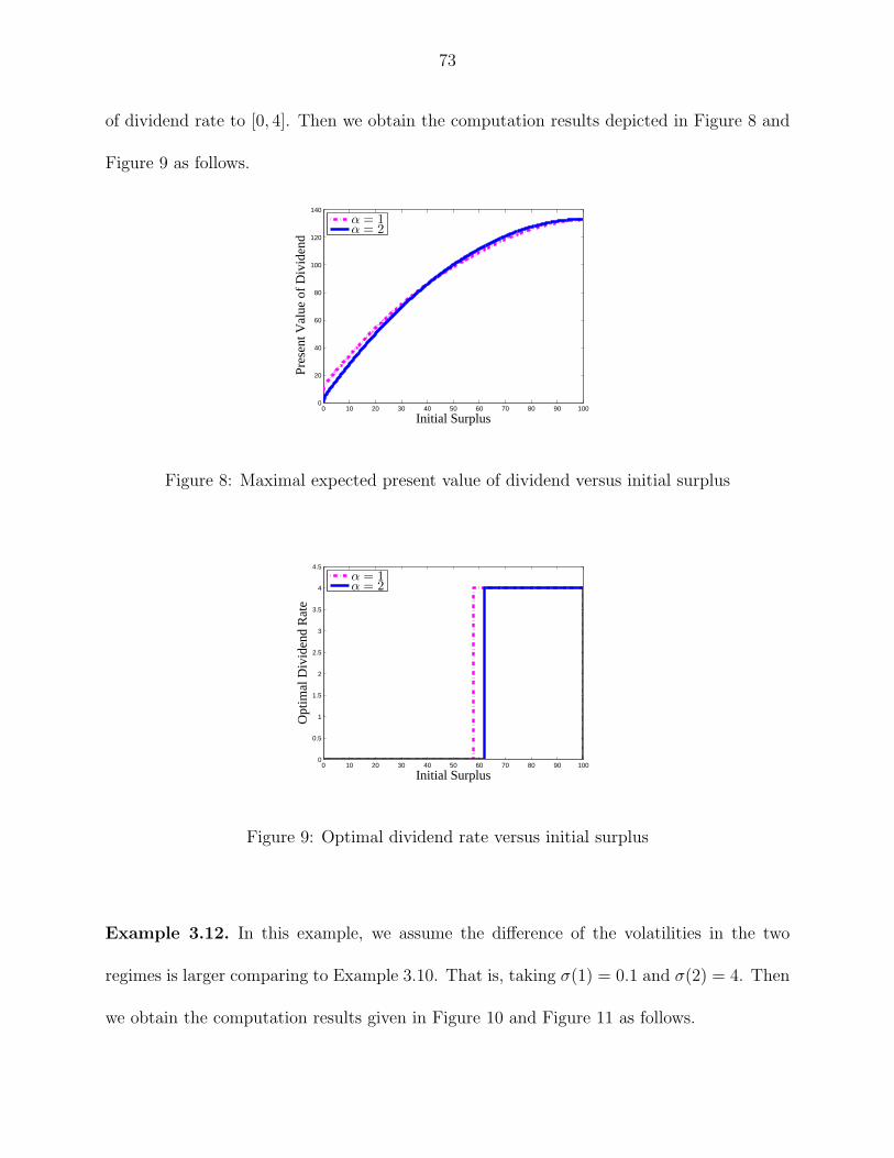
73

of dividend rate to [0, 4]. Then we obtain the computation results depicted in Figure 8 and

Figure 9 as follows.

0 10 20 30 40 50 60 70 80 90 1000

20

40

60

80

100

120

140

Initial Surplus

Pres

ent V

alue

of

Div

iden

d

α = 1α = 2

Figure 8: Maximal expected present value of dividend versus initial surplus

0 10 20 30 40 50 60 70 80 90 1000

0.5

1

1.5

2

2.5

3

3.5

4

4.5

Initial Surplus

Opt

imal

Div

iden

d R

ate

α = 1α = 2

Figure 9: Optimal dividend rate versus initial surplus

Example 3.12. In this example, we assume the difference of the volatilities in the two

regimes is larger comparing to Example 3.10. That is, taking σ(1) = 0.1 and σ(2) = 4. Then

we obtain the computation results given in Figure 10 and Figure 11 as follows.

74

0 10 20 30 40 50 60 70 80 90 1000

10

20

30

40

50

60

70

Initial Surplus

Pres

ent V

alue

of

Div

iden

d

α = 1α = 2

Figure 10: Maximal expected present value of dividend versus initial surplus

0 10 20 30 40 50 60 70 80 90 1000

0.5

1

1.5

2

2.5

3

3.5

4

4.5

Initial Surplus

Opt

imal

Div

iden

d R

ate

α = 1α = 2

Figure 11: Optimal dividend rate versus initial surplus

75

Figure 6 to Figure 11 show the expected present value of dividends versus initial surplus

and dividend rate versus initial surplus. From these figures, the expected present value of

dividends is an increasing function of the initial surplus, this is intuitively obvious. We can

also see that if the initial surplus is larger than certain level, the company should pay as

much dividend as allowable (this will result a threshold strategy due to the upper bound

of the dividend rate). From this we can deduce that, for t > 0, the optimal strategy for

Example 3.10 is a threshold strategy due to the restriction of maximum dividend rate being

less than the premium rate if the Markov chain is at state 2, and the optimal strategy for

Example 3.11 is a band strategy. The dividend is paid when Vx(x, i) < 1, in which case

the company is “inefficient” and cash surplus is high, otherwise, the company is considered

“efficient” when Vx(x, i) > 1. It is best to pay no dividend when the company is efficient

and the cash surplus is low, then funds should be left to company for growth.

By examining the graphs, the following observations are in order. Figure 6 and Figure

7, and Figure 8 and Figure 9 show that the dividend payment rates reach the thresholds

depending on the sign of Vx(x, i)− 1 no matter whether the ceiling of the dividend payment

rate is greater than premium rate or not. However, since the cap of dividend rate is larger

in Example 3.11, the dividend will be paid at the rate of premium rate. This will be a kind

band strategy. In Example 3.10, the cap of dividend rate is less than the premium rate if

the state is 2, this will lead to a threshold strategy.

In addition, the difference of volatilities in Example 3.10 is 1.8 and the difference of

volatilities in Example 3.12 is 3.9. From Figure 10 and Figure 11, we can see that the

difference of the dividend payment strategies is bigger comparing to Figure 6 and Figure 7,

in which case the difference of the volatilities is smaller. So the optimal dividend strategies

76

are sensitive to the market regimes. This indicates that the regime-switching models are

appropriate for the intended modeling and optimization.

77

4 Further Remarks

This dissertation has been devoted to numerical methods for problems arising in risk man-

agement and insurance. By choosing Markov regime-switching technique, the models are

more realistic but more complicate. More often than not, closed-form solutions are not

obtainable. Thus developing numerical solutions is necessary.

In Chapter 2, a numerical approximation scheme to minimize the probability of lifetime

ruin for annuity purchase, has been developed. Although one could derive the associate

systems of variational inequalities together with the use of properties of switching diffusions,

solving them analytically is very difficult. Thus a numerical approach for solving such prob-

lems is a necessary step. One may directly discretize the system of variational inequalities,

but this relies on the properties of the variational inequalities. We provide a viable alterna-

tive. Our Markov chain approximation method uses mainly probabilistic methods and does

not need any analytic properties of the solutions of the system of variational inequalities. In

the examples, for the constant hazard rate, we show that it is more advantage to purchase

the life annuity than self annuitization so that the individual will have less probability of

financial ruin even though he or she is less wealthy and maintains the same consumption.

For the more general hazard rate such as Gompertz, we show that the individual with the

same wealth but younger age will more likely to outlives his or her wealth.

In Chapter 3, we have developed a numerical approximation scheme to maximize the

present value of dividend with optimal dividend rate selection. Although one could derive

the associate system of HJB equations by using the usual dynamic programming approach

together with the use of properties of switching jump diffusions, solving them analytically

78

is very difficult. As an alternative, one may try to discretize the system of HJB equations

directly, but this relies on the properties of the HJB equations. As is mentioned above,

the powerful Markov chain approximation method could guarantee the consistent of the

interpolation sequence with the original dynamic system. In the actual computation, the

optimal control can be obtained by using the value or policy iteration methods.

For future study, singular control in dividend payout problem can be considered. For such

cases, the dividend payout rate could not be obtained. With the regime-switching technique,

we will need to consider the corresponding quasi-variational inequalities. Furthermore, one

may consider the Markov chain approximation method to study the numerical solution of

the optimal control policy.

79

REFERENCES

[1] S. Asmussen, B. Høgaard, and M. Taksar, Optimal risk control and dividend distribution

policies. Example of excess-of loss reinsurance for an insurance corporation. Finance and

Stochastics, 4 (2000), 299–324.

[2] S. Asmussen and M. Taksar, Controlled diffusion models for optimal dividend pay-Out.

Insurance: Math. and Economics, 20 (1997), 1–15.

[3] J.R. Brown, Private pensions, mortality risk, and the decision to annuitize, J. Public

Econ., 82 (2001), 29–62.

[4] B. De Finetti, Su unimpostazione alternativa della teoria collettiva del rischio. Trans-

actions of the XVth International Congress of Actuaries 2 (1957), 433–443.

[5] A. Cadenillas, T. Choulli, M. Taksar, and L. Zhang, Classical and impulse stochastic

control for the optimization of the dividend and risk policies of an insurance firm,

Mathematical Finance, 16 (2006), 181–202.

[6] T. Davidoff, J. Brown, and P. Diamond, Annuities and individual welfare, M.I.T. De-

partment of Economics Working Paper Series, Working Paper 03–15.

[7] G.B. Di Masi, Y.M. Kabanov, and W.J. Runggaldier, Mean variance hedging of options

on stocks with Markov volatility, Theory Probab. Appl., 39 (1994), 173–181.

[8] H. Gerber and E. Shiu, Optimal dividends: analysis with Brownian motion. North

American Actuarial Journal, 8 (2004), 1–20.

80

[9] H. Gerber and E. Shiu, On optimal dividend strategies in the compound Poisson model.

North American Actuarial Journal, 10 (2006), 76–93.

[10] M.K. Ghosh, A. Arapostathis and S.I. Marcus, Optimal control of switching diffusions

with application to flexible manufacturing systems, SIAM J. Control Optim., 31 (1993),

1183–1204.

[11] Z. Jin, G. Yin, Numerical Methods for Dividend Policy of Regime-Switching Jump-

Diffusion Models, to appear in International Journal of Computer Mathematics.

[12] S. Kapur and M. Orszag, A Portfolio Approach to Investment and Annuitization during

Retirement, Working Paper, Birkbeck College, University of London.

[13] H.J. Kushner and P. Dupuis, Numerical Methods for Stochastic Control Problems in

Continuous Time, 2nd Ed., Springer, New York, 2001.

[14] F. Lundberg. Approximerad Framstallning av Sannolikehetsfunktionen, Aterforsakering

av Kollektivrisker, Almqvist & Wiksell, Uppsala. Akad. Afhandling. Almqvist o. Wik-

sell, Uppsala, 1903.

[15] M. Milevsky, K. Moore, and V. R .Young, Asset allocation and annuity-purchase s-

trategies to minimize the probability of financial ruin, Mathematical Finance, 16 2006,

647–671.

[16] S. Richard, Optimal Consumption, portfolio and life insurance rules for an uncertain

lived individual in a continuous time model, J. Financ. Econ., 2 (1975), 187–203.

[17] H. Schmidli, Stochastic Control in Insurance. Springer Verlag, 2008.

81

[18] Q. S. Song, G. Yin, and Z. Zhang, Numerical method for controlled regime-switching

diffusions and regime-switching jump diffusions, Automatica, 42 (2006), 1147–1157.

[19] L. Sotomayor and A. Cadenillas, Classical, Singular, and Impulse Stochastic Control

for the Optimal Dividend Policy when There is Regime Switching. Preprint, (2008),

Download at http://papers.ssrn.com/sol3/papers.cfm?abstract-id=1139444.

[20] M. Yaari, Uncertain lifetime, life insurance and the theory of the consumer, Review of

Economic Studies 32,

[21] M. Yaari (1965). Uncertain lifetime, life insurance and the theory of the consumer,

Review of Economic Studies, 32, (1965) 137C150.

[22] G. Yin, V. Krishnamurthy, and C. Ion, Regime switching stochastic approximation al-

gorithms with application to adaptive discrete stochastic optimization, SIAM J. Optim.,

14 (2004), 1187–1215.

[23] G. Yin and C. Zhu, Hybrid Switching Diffusions: Properties and Applications, Springer,

New York, 2010.

[24] G. Yin, Q. Zhang, and G. Badowski, Discrete-time singularly perturbed Markov chains:

Aggregation, occupation measures, and switching diffusion limit, Adv. Appl. Probab. 35

(2003), 449–476.

[25] V.R. Young, Optimal investment strategy to minimize the probability of lifetime ruin,

N. Amer. Actuarial J., 8 (2004), 106–126.

82

[26] Q. Zhang, Stock trading: An optimal selling rule, SIAM J. Control Optim, 40 (2001),

64–87.

[27] X.Y. Zhou and G. Yin, Markowitz mean-variance portfolio selectionwith regime switch-

ing: A continuous-time model, SIAM J. Control Optim, 42 (2003), 1466–1482.

83

ABSTRACT

NUMERICAL METHODS FOR PROBLEMS ARISING IN

RISK MANAGEMENT AND INSURANCE

by

ZHUO JIN

August 2011

Advisor: Dr. G. George Yin

Major: Mathematics (Applied)

Degree: Doctor of Philosophy

In this dissertation we investigate numerical methods for problems annuity purchasing

and dividend optimization arising in risk management and insurance. We consider the models

with Markov regime-switching process. The regime-switching model contains both continu-

ous and discrete components in their evolution and is referred to as a hybrid system. The

discrete events are used to model the random factors that cannot formulated by differential

equations. The switching process between regimes is modulated as a finite state Markov

chain.

As is widely recognized, this regime-switching model appears to be more versatile and

more realistic. However, because of the regime switching and the nonlinearity, it is virtually

impossible to obtain closed-form or analytic solutions for our problems. Thus we are seeking

numerical solutions by using Markov chain approximation methods.

Focusing on numerical solutions of the regime-switching models in the area of actuarial

science, and based on the theory of weak convergence of probability measures, the conver-

gence of the approximating sequences is obtained. In fact, under very broad conditions,

we prove that the sequences of approximating Markov chain, the cost functions, and the

value functions all converge to that of the underlying original processes. The proofs are

84

purely probabilistic. It need not appeal to regularity properties of or even explicitly use the

Bellman equation. Moreover, the feasibility of regime-switching model and Markov chain

approximation method are illustrated by the examples.

85

AUTOBIOGRAPHICAL STATEMENT

ZHUO JIN

Education

• Ph.D. in Applied Mathematics, December 2011 (expected)Wayne State University, Detroit, Michigan

• M.A. in Mathematical Statistics, May, 2010Wayne State University, Detroit, Michigan

• B.S. in Applied Mathematics, June 2005Huazhong University of Science and Technology, Wuhan, China

Awards

1. The Alfred L. Nelson Award in Recognition of Outstanding Achievement, Departmentof Mathematics, Wayne State University, April 2011.

2. The Maurice J. Zelonka Endowed Mathematics Scholarship, Department of Mathe-matics, Wayne State University, April 2010.

3. Graduate Student Professional Travel Award, Department of Mathematics, WayneState University, August 2010.

List of Publications

1. Zhuo Jin, G. Yin, and H.L. Yang, Numerical methods for dividend optimization usingregime-switching jump-diffusion models, Mathematical Control and Related Fields, 1(2011), 21-40.

2. Zhuo Jin, Yumin Wang, and G. Yin, Numerical solutions of quantile hedging for guar-anteed minimum death benefits under a regime-switching-jump-diffusion formulation,Journal of Computational and Applied Mathematics, 235 (2011) 2842-2860.

3. Zhuo Jin, G. Yin, A numerical method for annuity-purchasing decision making to mini-mize the probability of financial ruin for regime-switching wealth Models, InternationalJournal of Computer Mathematics, 88 (2011), 1256-1282.

4. G. Yin, Zhuo Jin, and H.L. Yang, Asymptotically optimal dividend policy for regime-switching compound Poisson models, Acta Mathematicae Applicatae Sinica, 26 (2010),529-542.

5. G. Yin, H. Jin, and Zhuo Jin, Numerical methods for portfolio selection with boundedconstraints, Journal of Computational and Applied Mathematics, 233 (2009), 564-581.