numerical methods for nonlinear pdeâ s in financeweb.math.ku.dk/noter/filer/phd15sm.pdf · in...
TRANSCRIPT

University of Copenhagen
PhD Thesis
Numerical Methods for Nonlinear PDEsin Finance
Author:
Sima Mashayekhi
This thesis submitted in fulfilment of the requirements
for the degree of Doctor of Philosophy
in the
Department of Mathematical Sciences
University of Copenhagen
September 2015

Sima Mashayekhi
Department of Mathematical Sciences
University of Copenhagen
Universitetsparken 5
DK-2100 Købehavn Ø
Denmark
PhD thesis submitted to the PhD School of Science, Faculty of Science, University of Copen-
hagen, Denmark, in September 2015.
Academic advisors: Jens Hugger
University of Copenhagen, Denmark
Rolf Poulsen
University of Copenhagen, Denmark
Assessment Committee: Trine Krogh Boomsma (chair)
University of Copenhagen, Denmark
Lina von Sydow
Uppsala University, Sweden
David Skovmand
Copenhagen Business School, Denmark
c© Sima Mashayekhi, 2015, except for the following articles:
Paper 1 (Chapter 2): Kα-Shifting, Rannacher Time Stepping and Mesh Grading in Crank Nicol-
son FDM for Black-Scholes Option Pricing
c©Sima Mashayekhi and Jens Hugger
Paper 2 (Chapter 3): Standard Finite Difference Schemes for European Options
Paper 3 (Chapter 4): Feedback Options in Nonlinear Numerical Finance
c©Jens Hugger and Sima Mashayekhi
Paper 4 (Chapter 5): Finite Difference Schemes for a Nonlinear Black-Scholes Model with Trans-
action Cost and Volatility Risk
c©Sima Mashayekhi and Jens Hugger
ISBN 978-87-7078-935-6

Abstract
Nonlinear Black-Scholes equations arise from considering parameters such as feedback
and illiquid markets effects or large investor preferences, volatile portfolio and nontrivial
transaction costs into option pricing models to have more accurate option price. Here
some finite difference schemes have been investigated to solve numerically such nonlinear
equations.
However the analytical solution of the linear Black-Scholes equation is known, different
numerical methods have been considered for solving the equation to make a general nu-
merical scheme for solving other more complicated models with no analytical solutions
such as nonlinear Black-Scholes models. Therefore at first some investigations for the
standard linear Black-Scholes equation have been considered for instance choosing a suit-
able right boundary condition and applying some remedies for dealing with nonsmooth
conditions of the equation. After that a number of nonlinear Black-Scholes models are
reviewed and different numerical methods have been investigated for solving some of
those models. At the end the numerical schemes have been compared with respect to
order of convergence.

Acknowledgements
I would like to express my special appreciation and thanks to my supervisors Jens Hugger
and Rolf Poulsen for their supports, ideas and encouraging my research. In particular,
I thank Jens for his enthusiasm and invaluable advices, and Rolf for his insightful com-
ments. I also sincerely thank Jeffrey S. Scroggs who provided me an opportunity to have
a great experience of visiting North Carolina State University and doing some research
during my five months stay abroad. Moreover, I would like to thank my committee
members for their comments and suggestions.
A special thanks to my family. Words cannot express how grateful I am to my par-
ents for their all kindness and support. I would also like to thank all of my friends,
colleagues and the rest of the department of Mathematics for this great experience that
I had during this recent years. At the end I would like express appreciation to my little
daughter Saba for giving us a nicer life and especially my beloved husband who was
always my support in the moments when there was no one to answer my queries.
September 2015
Copenhagen, Denmark
Sima Mashayekhi
iv

List of Papers
This thesis is based on the following four papers:
• Sima Mashayekhi and Jens Hugger, Kα-Shifting, Rannacher Time Stepping and
Mesh Grading in Crank-Nicolson FDM for Black-Scholes Option Pricing, To be
appeared in Journal of Communications in Mathematical Finance (CMF), (2015).
• Jens Hugger and Sima Mashayekhi, Standard Finite Difference Schemes for Eu-
ropean Options, Working Paper, (2015).
• Jens Hugger and Sima Mashayekhi, Feedback Options in Nonlinear Numerical Fi-
nance, International Conference of Numerical Analysis and Applied Mathematics.
AIP Conference Proceedings, Volume 1479 (2012) pp. 2266-2269.
• Sima Mashayekhi and Jens Hugger, Finite Difference Schemes for a Nonlinear
Black-Scholes Model with Transaction Cost and Volatility Risk, Acta Mathematica
Universitatis Comenianae (AMUC), Vol 84, No 2 (2015), pp. 255-266.
v


Contents
Abstract iii
Acknowledgements iv
List of Papers v
List of Figures xi
List of Tables xiii
Abbreviations xvii
Symbols xix
1 Introduction 1
1.1 Linear Black-Scholes Model . . . . . . . . . . . . . . . . . . . . . . . . . . 1
1.1.1 PDE model of European vanilla options on unbounded domain . . 2
1.1.2 Solutions and Greeks . . . . . . . . . . . . . . . . . . . . . . . . . . 4
1.1.3 Limits . . . . . . . . . . . . . . . . . . . . . . . . . . . . . . . . . . 9
1.1.4 Differential equation on a bounded domain . . . . . . . . . . . . . 11
1.1.5 Transformations of differential equation . . . . . . . . . . . . . . . 12
1.1.6 Numerical methods for solving European option on bounded domain 13
1.2 Nonlinear Black-Scholes Models . . . . . . . . . . . . . . . . . . . . . . . . 16
1.2.1 Leland Model . . . . . . . . . . . . . . . . . . . . . . . . . . . . . . 17
1.2.2 Risk Adjusted Pricing Methodology(RAPM) . . . . . . . . . . . . 18
1.2.3 Barles and Soner model . . . . . . . . . . . . . . . . . . . . . . . . 18
1.2.4 Feedback and illiquid market . . . . . . . . . . . . . . . . . . . . . 19
1.2.5 Parameterized Illiquidity Model . . . . . . . . . . . . . . . . . . . . 20
2 Kα-Shifting, Rannacher Time Stepping and Mesh Grading in CrankNicolson FDM for Black-Scholes Option Pricing 23
2.1 Introduction . . . . . . . . . . . . . . . . . . . . . . . . . . . . . . . . . . . 24
2.2 Kα-shifting . . . . . . . . . . . . . . . . . . . . . . . . . . . . . . . . . . . 27
2.2.1 Stability of Kα with respect to the interest rate . . . . . . . . . . . 35
2.2.2 Stability of Kα with respect to the volatility . . . . . . . . . . . . 36
2.3 Kα-shifting, Rannacher time stepping and mesh grading . . . . . . . . . . 37
2.4 Order of Convergence . . . . . . . . . . . . . . . . . . . . . . . . . . . . . 45
vii

Contents viii
2.5 Conclusions and future work . . . . . . . . . . . . . . . . . . . . . . . . . 48
Appendices 51
2.A Grid Stretching . . . . . . . . . . . . . . . . . . . . . . . . . . . . . . . . . 51
3 Standard Finite Difference Schemes for European Options 53
3.1 Introduction . . . . . . . . . . . . . . . . . . . . . . . . . . . . . . . . . . . 54
3.2 Numerical results for the explicit Euler method . . . . . . . . . . . . . . . 56
3.2.1 Computational results for the standard case . . . . . . . . . . . . . 56
3.2.2 Computational results for nonstandard cases . . . . . . . . . . . . 62
3.2.3 Sensitivity to Smax . . . . . . . . . . . . . . . . . . . . . . . . . . 67
3.2.4 Convergence . . . . . . . . . . . . . . . . . . . . . . . . . . . . . . 68
3.2.5 Volatility limit . . . . . . . . . . . . . . . . . . . . . . . . . . . . . 77
3.2.6 Expiration limit . . . . . . . . . . . . . . . . . . . . . . . . . . . . 81
3.3 Numerical results for the backward Euler method . . . . . . . . . . . . . . 83
3.3.1 Computational results for the standard case . . . . . . . . . . . . . 83
3.3.2 Computational results for nonstandard cases . . . . . . . . . . . . 88
3.3.3 Sensitivity to Smax . . . . . . . . . . . . . . . . . . . . . . . . . . 91
3.3.4 Convergence . . . . . . . . . . . . . . . . . . . . . . . . . . . . . . 91
3.3.5 Volatility limit . . . . . . . . . . . . . . . . . . . . . . . . . . . . . 96
3.3.6 Expiration limit . . . . . . . . . . . . . . . . . . . . . . . . . . . . 99
3.4 Numerical results for the Crank Nicolson method . . . . . . . . . . . . . . 100
3.4.1 Computational results for the standard case . . . . . . . . . . . . . 100
3.4.2 Computational results for nonstandard cases . . . . . . . . . . . . 104
3.4.3 Sensitivity to Smax . . . . . . . . . . . . . . . . . . . . . . . . . . . 107
3.4.4 Convergence . . . . . . . . . . . . . . . . . . . . . . . . . . . . . . 107
3.4.5 Volatility limit . . . . . . . . . . . . . . . . . . . . . . . . . . . . . 112
3.4.6 Expiration limit . . . . . . . . . . . . . . . . . . . . . . . . . . . . 114
3.5 Conclusion . . . . . . . . . . . . . . . . . . . . . . . . . . . . . . . . . . . 115
4 Feedback Options in Nonlinear Numerical Finance 117
4.1 Introduction . . . . . . . . . . . . . . . . . . . . . . . . . . . . . . . . . . . 117
4.2 Literature survey on illiquid markets and feedback options . . . . . . . . . 118
4.3 PDE model for feedback options on an unbounded and on a boundeddomain . . . . . . . . . . . . . . . . . . . . . . . . . . . . . . . . . . . . . 120
4.4 Numerical methods for solving the feedback options . . . . . . . . . . . . 122
4.5 Numerical results and conclusions . . . . . . . . . . . . . . . . . . . . . . . 124
5 Finite Difference Schemes for a Nonlinear Black-Scholes Model withTransaction Cost and Volatility Risk 129
5.1 Introduction . . . . . . . . . . . . . . . . . . . . . . . . . . . . . . . . . . . 130
5.2 The Barles and Soner nonlinear volatility model . . . . . . . . . . . . . . . 131
5.3 Finite Difference Schemes . . . . . . . . . . . . . . . . . . . . . . . . . . . 132
5.4 Numerical Results . . . . . . . . . . . . . . . . . . . . . . . . . . . . . . . 134
5.5 Conclusions . . . . . . . . . . . . . . . . . . . . . . . . . . . . . . . . . . . 141
Appendices 143
5.A NFDM Scheme . . . . . . . . . . . . . . . . . . . . . . . . . . . . . . . . . 143

Contents ix
5.B NFDM Perperties Theorem . . . . . . . . . . . . . . . . . . . . . . . . . . 148
5.C Ψ(x) Plot . . . . . . . . . . . . . . . . . . . . . . . . . . . . . . . . . . . . 151
Bibliography 153


List of Figures
1.1 Solutions to options at start and expiration . . . . . . . . . . . . . . . . . 5
1.2 Solutions to options from start to expiration . . . . . . . . . . . . . . . . . 5
1.3 Deltas for different options at start and expiration . . . . . . . . . . . . . 6
1.4 Deltas for different options from start to expiration . . . . . . . . . . . . . 7
1.5 Gamma for different options at start and expiration . . . . . . . . . . . . 7
1.6 Gammas for different options from start to expiration . . . . . . . . . . . 8
2.1 CN 3D error for call, bet and butterfly spread with different meshes . . . 25
2.2 Maximal CN error as a function of Kα for call and bet options . . . . . . 31
2.3 Maximal CN error as a function of Kα for Greeks . . . . . . . . . . . . . . 33
2.4 Maximal CN error as a function of Kα and r for call and bet options . . . 36
2.5 Maximal CN error as a function of Kα and σ for call and bet options . . . 37
2.6 CNGS, CNRGS, CNKGS and CNRKGS errors for bet option . . . . . . . 39
2.7 CN, CNR, CNK and CNRK errors for bet option . . . . . . . . . . . . . . 40
2.8 CN, CNR, CNK and CNRK errors for Delta bet . . . . . . . . . . . . . . 41
2.9 CN, CNR, CNK and CNRK errors for Gamma bet . . . . . . . . . . . . . 42
2.10 Maximal errors for options and Greeks with different meshes and schemes 44
2.11 3D plot of CN, CNR, CNK, CNRKα maximal error for bet option . . . . 46
2.A.1position of nodal points with grid stretching transformation . . . . . . . . 52
3.2.1 FE coarse mesh error for put option with different Smax . . . . . . . . . . 59
3.2.2 FE fine mesh error for put option with different Smax . . . . . . . . . . . 60
3.2.3 FE error for put option with coarse and fine meshes and different T . . . 65
3.2.4 3D plot of FE maximal error for put option . . . . . . . . . . . . . . . . . 69
3.2.5 FE 3D error for put option with different meshes . . . . . . . . . . . . . . 70
3.2.6 3D plot of FE maximal error for call option . . . . . . . . . . . . . . . . . 71
3.2.7 3D plot of FE maximal error for bet option . . . . . . . . . . . . . . . . . 72
3.2.8 FE 3D error for bet option with different meshes . . . . . . . . . . . . . . 73
3.2.9 3D plot of FE maximal error for smoothened put option . . . . . . . . . . 74
3.2.10FE 3D error for smoothened put option with different meshes . . . . . . . 75
3.2.11FE error coarse mesh for put option with different volatility . . . . . . . . 79
3.2.12FE error fine mesh for put option with different volatility . . . . . . . . . 80
3.3.1 BE coarse mesh error for put option with different Smax . . . . . . . . . . 85
3.3.2 BE fine mesh error for put option with different Smax . . . . . . . . . . . 86
3.3.3 BE error for put option with coarse and fine meshes and different T . . . 90
3.3.4 3D plot of BE maximal error for put option . . . . . . . . . . . . . . . . . 92
3.3.5 BE 3D error for put option with different meshes . . . . . . . . . . . . . . 93
3.3.6 3D plot of BE maximal error for call option . . . . . . . . . . . . . . . . . 94
xi

List of Figures xii
3.3.7 3D plot of BE maximal error for bet option . . . . . . . . . . . . . . . . . 95
3.3.8 3D plot of BE maximal error for smoothened put option . . . . . . . . . . 96
3.3.9 BE error fine mesh for put option with different volatility . . . . . . . . . 98
3.4.1 CN coarse mesh error for put option with different Smax . . . . . . . . . . 102
3.4.2 CN fine mesh error for put option with different Smax . . . . . . . . . . . 103
3.4.3 CN error for put option with coarse and fine meshes and different T . . . 106
3.4.4 3D plot of CN maximal error for put option . . . . . . . . . . . . . . . . . 108
3.4.5 CN 3D error for put option with different meshes . . . . . . . . . . . . . . 109
3.4.6 3D plot of CN maximal error for call option . . . . . . . . . . . . . . . . . 110
3.4.7 3D plot of CN maximal error for bet option . . . . . . . . . . . . . . . . . 111
3.4.8 Put option with different volatility solved with CN . . . . . . . . . . . . . 113
4.1 First-order and full feedback call option . . . . . . . . . . . . . . . . . . . 127
5.1 Nonlinear put option solved with NFDM . . . . . . . . . . . . . . . . . . . 136
5.2 NFDM and FtCS stability region with different transaction cost parameters137
5.3 Local errors for nonlinear call and bet options solved with different schemes138
5.4 Global errors for nonlinear call option solved with different schemes . . . 139
5.C.1The Barles and Soner Ψ function satisfying (5.5). . . . . . . . . . . . . . . 151

List of Tables
2.1 Optimal Kα for butterfly spread solution and Greeks . . . . . . . . . . . . 34
2.2 CN, CNR, CNKα and CNRKα maximal error for bet option and Greeks . 42
3.2.1 FE maximal error for put option with Smax ' 4K . . . . . . . . . . . . . 57
3.2.2 FE maximal error for put option with Smax ' 2K . . . . . . . . . . . . . 57
3.2.3 FE maximal error for put option with Smax ' 1.5K . . . . . . . . . . . . 58
3.2.4 FE maximal error for put option with Smax ' 1.25K . . . . . . . . . . . . 58
3.2.5 FE maximal error for call option with Smax ' 4K . . . . . . . . . . . . . 61
3.2.6 FE maximal error for bet option with Smax ' 4K . . . . . . . . . . . . . . 61
3.2.7 FE maximal error for smoothened put option with different Smax . . . . . 62
3.2.8 FE maximal error for smoothened put option with Smax ' 30K . . . . . . 62
3.2.9 Smallest Smax not giving significant FE error at S = Smax for put optionwith a coarse mesh and different parameters . . . . . . . . . . . . . . . . . 63
3.2.10Smallest Smax not giving significant FE error at S = Smax for put optionwith a course mesh and different γ . . . . . . . . . . . . . . . . . . . . . . 63
3.2.11Smallest Smax not giving significant FE error at S = Smax for put optionwith a fine mesh and different parameters . . . . . . . . . . . . . . . . . . 64
3.2.12Smallest Smax not giving significant FE error at S = Smax for put optionwith a fine mesh and different γ . . . . . . . . . . . . . . . . . . . . . . . . 64
3.2.13Smallest Smax not giving significant FE error at S = Smax for call optionwith a course mesh and different parameters . . . . . . . . . . . . . . . . . 66
3.2.14Smallest Smax not giving significant FE error at S = Smax for call optionwith a course mesh and different γ . . . . . . . . . . . . . . . . . . . . . . 66
3.2.15Smallest Smax not giving significant FE error at S = Smax for bet optionwith a course mesh and different parameters . . . . . . . . . . . . . . . . . 66
3.2.16Smallest Smax not giving significant FE error at S = Smax for bet optionwith a course mesh and different γ and B . . . . . . . . . . . . . . . . . . 67
3.2.17FE maximal error for put option with different σ . . . . . . . . . . . . . . 77
3.2.18FE maximal error for put option at t = T − dt . . . . . . . . . . . . . . . 81
3.2.19FE maximal error for put option at t = T − 5dt . . . . . . . . . . . . . . . 81
3.2.20FE maximal error for call option at t = T − dt . . . . . . . . . . . . . . . 81
3.2.21FE maximal error for call option at t = T − 5dt . . . . . . . . . . . . . . . 81
3.2.22FE maximal error for bet option at t = T − dt . . . . . . . . . . . . . . . 81
3.2.23FE maximal error for bet option at t = T − 5dt . . . . . . . . . . . . . . . 82
3.2.24FE maximal error for smoothened put option at t = T − dt . . . . . . . . 82
3.2.25FE maximal error for smoothened put option at t = T − 5dt . . . . . . . . 82
3.3.1 BE maximal error for put option with Smax ' 4K . . . . . . . . . . . . . 83
3.3.2 BE maximal error for put option with Smax ' 2K . . . . . . . . . . . . . 84
xiii

List of Tables xiv
3.3.3 BE maximal error for put option with Smax ' 1.5K . . . . . . . . . . . . 84
3.3.4 BE maximal error for put option with Smax ' 1.25K . . . . . . . . . . . . 84
3.3.5 BE maximal error for call option with Smax ' 4K . . . . . . . . . . . . . 87
3.3.6 BE maximal error for bet option with Smax ' 4K . . . . . . . . . . . . . . 87
3.3.7 BE maximal error for smoothened put option with Smax ' 30K . . . . . . 88
3.3.8 Smallest Smax not giving significant BE error at S = Smax for put optionwith a coarse mesh and different parameters . . . . . . . . . . . . . . . . . 89
3.3.9 Smallest Smax not giving significant BE error at S = Smax for put optionwith a coarse mesh and different γ . . . . . . . . . . . . . . . . . . . . . . 89
3.3.10Smallest Smax not giving significant BE error at S = Smax for put optionwith a fine mesh and different parameters . . . . . . . . . . . . . . . . . . 89
3.3.11Smallest Smax not giving significant BE error at S = Smax for put optionwith a fine mesh and different γ . . . . . . . . . . . . . . . . . . . . . . . . 90
3.3.12BE maximal error for put option with different σ . . . . . . . . . . . . . . 97
3.3.13BE maximal error for put option at t = T − dt . . . . . . . . . . . . . . . 99
3.3.14BE maximal error for put option at t = T − 5dt . . . . . . . . . . . . . . . 99
3.3.15BE maximal error for call option at t = T − dt . . . . . . . . . . . . . . . 99
3.3.16BE maximal error for call option at t = T − 5dt . . . . . . . . . . . . . . . 99
3.3.17BE maximal error for bet option at t = T − dt . . . . . . . . . . . . . . . 99
3.3.18BE maximal error for bet option at t = T − 5dt . . . . . . . . . . . . . . . 100
3.4.1 CN maximal error for put option with Smax ' 4K . . . . . . . . . . . . . 100
3.4.2 CN maximal error for put option with Smax ' 2K . . . . . . . . . . . . . 101
3.4.3 CN maximal error for put option with Smax ' 1.5K . . . . . . . . . . . . 101
3.4.4 CN maximal error for put option with Smax ' 1.25K . . . . . . . . . . . . 101
3.4.5 CN maximal error for call option with Smax ' 4K . . . . . . . . . . . . . 104
3.4.6 CN maximal error for bet option with Smax ' 4K . . . . . . . . . . . . . 104
3.4.7 Smallest Smax not giving significant CN error at Smax for put option witha coarse mesh and different parameters . . . . . . . . . . . . . . . . . . . . 105
3.4.8 Smallest Smax not giving significant CN error at S = Smax for put optionwith a coarse mesh and different γ . . . . . . . . . . . . . . . . . . . . . . 105
3.4.9 Smallest Smax not giving significant CN error at Smax for put option witha fine mesh and different parameters . . . . . . . . . . . . . . . . . . . . . 107
3.4.10Smallest Smax not giving significant CN error at S = Smax for put optionwith a fine mesh and different γ . . . . . . . . . . . . . . . . . . . . . . . . 107
3.4.11CN maximal error for put option with different σ . . . . . . . . . . . . . . 112
3.4.12CN maximal error for put option at t = T − dt . . . . . . . . . . . . . . . 114
3.4.13CN maximal error for put option at t = T − 5dt . . . . . . . . . . . . . . . 114
3.4.14CN maximal error for call option at t = T − dt . . . . . . . . . . . . . . . 114
3.4.15CN maximal error for call option at t = T − 5dt . . . . . . . . . . . . . . . 114
3.4.16CN maximal error for bet option at t = T − dt . . . . . . . . . . . . . . . 114
3.4.17CN maximal error for bet option at t = T − 5dt . . . . . . . . . . . . . . . 115
4.1 First-order feedback error in a coarse mesh . . . . . . . . . . . . . . . . . 125
4.2 First-order feedback error in a fine mesh . . . . . . . . . . . . . . . . . . . 125
4.3 Full feedback error in a coarse mesh . . . . . . . . . . . . . . . . . . . . . 125
4.4 Full feedback error in a fine mesh . . . . . . . . . . . . . . . . . . . . . . . 125

List of Tables xv
5.1 Convergence results for the nonlinear call option solved with NFDM andFtCS . . . . . . . . . . . . . . . . . . . . . . . . . . . . . . . . . . . . . . . 138
5.2 Convergence results for the nonlinear call option solved with CNR andPosPre . . . . . . . . . . . . . . . . . . . . . . . . . . . . . . . . . . . . . . 139


Abbreviations
BE Backward Euler
B-S Black Scholes
BVP Boundary Value Problem
BS Black Scholes
CN Crank Nicolson
CNK Crank Nicolson Kα-optimization
CNGS Crank Nicolson Grid Stretching
CNR Crank Nicolson Rannacher
FDM Finite Difference Method
FE Forward Euler
FtCS Forward in time Central in S
ImpUp Implicit Upwind
NFDM Nonstandard Finite Difference Method
PDE Partial Differencial Equation
PosPre Positive Preserving
xvii


Symbols
S underlying risky asset
t time
T terminal time
γ dividend yield
σ volatility of the underlying risky asset
r market interest rate
K strike price (exercise price)
B Bet
H Heaviside function
xix


Chapter 1
Introduction
This thesis except this chapter as a general introduction consist of four chapters that
are written as academic articles on different topics and therefore are self-contained. In
this chapter an overview of linear and nonlinear Black-Scholes models, definitions and
properties of the models are given. Some remedies to deal with non-smooth condition of
the Black-Scholes equation has been investigated in Chapter 2 to restore the convergence
order of the Crank Nicolson. In Chapter 3 some standard finite difference schemes
have been considered for European option pricing and position of Smax as the right
boundary condition of the Black-Scholes equation is considered. After investigation on
linear Black-Scholes equation two different nonlinear Black-Scholes equations have been
investigated in Chapters 4 and 5.
1.1 Linear Black-Scholes Model
The standard Black-Scholes model is a well known linear equation derived by Fischer
Black and Myron Scholes in 1973 [5] and earlier by Robert Merton [33] for pricing options
in financial derivatives. Standard finite difference schemes for solving the partial differ-
ential equation formulation of European vanilla options are standard textbook material
today — see for example [11, 46, 26, 42]. Moreover numerous articles have investigated
this area — for instance [7, 9, 10, 13, 35, 43, 45].
1

Chapter 1. Introduction 2
In section 1.1.1 we present the partial differential equation model for the European
vanilla option on the unbounded domain and derive boundary conditions to be used for
numerical solution on a bounded domain.
One of the main obstacles in numerical option pricing is the fact that the terminal condi-
tion at the expiration time for the option in general contains one or more discontinuities
either in the option value (this is the case for example for the “cash or nothing call” or
simply the bet option with one discontinuity or butterfly spread with three discontinu-
ities) or in some derivatives of this (as for example for the put and call options having
discontinuities in the first derivative of the option value with respect to the risky asset
price S. This derivative is commonly denoted the option ∆). All finite difference meth-
ods involves solving the model PDE only in a finite number of mesh points. It turns
out that the error committed with the various methods depends on the position of the
discontinuity with respect to these mesh points.
Following research questions have been posed where have been answered in Chapters 2
and 3:
(1) How should the discontinuity be positioned with respect to the mesh points in order
to obtain the minimal error for the various options and methods?
(2) How does these discontinuities influence the convergence properties of various nu-
merical methods?
1.1.1 PDE model of European vanilla options on unbounded domain
The classical boundary value problem for a European option posed over the financially
relevant domain Ω∞ = (S, t) ∈]0,∞[×]0, T [ is found in most of the references in
section 1.1 to be the following terminal value problem:
Find V : (S, t) ∈ Ω∞ → R, V ∈ C0(Ω∞) ∩ C2,1(Ω∞) so that
∂V
∂t+
1
2σ2S2∂
2V
∂S2+ (r − γ)S
∂V
∂S− rV = 0 in Ω∞
and V (S, T ) is payoff function as the terminal condition in Ω∞|t=T . (1.1)
Here the dependent variable V (S, t) is the value (price) of the option for a value S of the
risky asset at time t. γ, σ > 0 and r — the dividend yield, volatility (on the underlying

Chapter 1. Introduction 3
risky asset) and market interest rate (on the riskfree asset) — are all assumed to be
independent of the value S of the underlying risky asset and time t in the standard
Black-Scholes model. The payoff is negotiated at time 0 between the buyer and seller of
the option. We shall here consider 4 simple options:
1. The put option where at time t = 0 it is agreed that you (the buyer of the option)
at time t = T may sell the underlying risky asset at the Strike Price K to your
opponent (the seller of the option) or you may choose to do nothing. This means
that at expiry you get a profit of — and hence the value V P of the option at expiry
is — V P (S(T ), T ) = maxK − S(T ), 0.
2. The call option is another very common option where at time t = 0 it is agreed
that you (the buyer of the option) at time t = T may buy the underlying risky
asset at the Strike Price K from your opponent (the seller of the option) or you
may choose to do nothing. This means that at expiry you get a profit of — and
hence the value V C of the option at expiry is — V C(S(T ), T ) = maxS(T )−K, 0.
3. The cash-or-nothing call option or the (Simple) Bet Option is an option where at
time t = 0 it is agreed that you (the buyer of the option) at time t = T get a lump
sum of B (the Bet) from your opponent (the seller of the option) if at that time,
the price of the risky asset is at least equal to the Strike Price K. This means that
at expiry you get a profit of — and hence the value V B of the option at expiry is
— V B(S(T ), T ) = BH(S(T )−K) where H(x) =
1 for x ≥ 0
0 for x < 0is the Heaviside
function.
4. The smoothened put option is introduced to serve as a reference in the investigation
of the above options. A main feature of the put, call and bet options are the
singularities in the terminal conditions at S = K.1 For the smoothened put option
we use the smooth terminal condition V SP (S(T ), T ) = K Smax−S(T )Smax
e−2S(T ). Here
1Note that for the put and call options, the value functions V P (·, T ) and V C(·, T ) are continuous
whereas ∂V P
∂S(·, T ) and ∂V C
∂S(·, T ) are discontinuous as functions of S (at S = K), i.e. V P (·, T ) ∈
C0(]0,∞[) and V C(·, T ) ∈ C0(]0,∞[) while we have a singularity in the first derivative at expiry. Insteadfor the bet option V B(·, T ) is discontinuous at S = K, so that we have a singularity already in thefunction value at expiry. The bet option is included in order to investigate the influence of discontinuitiesin the payoff on the solution V . It is well known that even a finite number of discontinuities in theterminal or boundary conditions to a linear parabolic differential equation problem [DEP] does notdestroy the infinite smoothness of the solution in the interior of the domain as long as the coefficientsof the derivatives are smooth. (See for example [22] §3.1).

Chapter 1. Introduction 4
Smax is the upper bound on the computational domain in the S variable, to be
introduced in more details later.
We shall use similar notation for any other relevant function such as V P , V C , V B, V SP
and V for the value function, ∆P , ∆C , ∆B, ∆SP and ∆ for the Delta-greek and so
on. For some predetermined strike price K, bet B and Smax we shall consider different
values of the 6 parameters T , K, B, r, γ and σ. However we shall define a Standard
Case with the parameters T = 1, K = 1, B = 0.3, r = 0.04, γ = 0 and σ = 0.2.
1.1.2 Solutions and Greeks
For our first 3 option cases the option prices V are known from basic finance text books
as for example [46] §5.4–5.5 (for γ = 0), [29] §2.2 (for put and call) or [20] §1.1.6 and
§2.11.2 (for all cases) and are given by
V P (S, t) = Ke−r(T−t)N(−d2)− e−γ(T−t)SN(−d1), (1.2)
V C(S, t) = −Ke−r(T−t)N(d2) + e−γ(T−t)SN(d1), (1.3)
V B(S, t) = Be−r(T−t)N(d2), (1.4)
where N(d) =1√2π
∫ d
−∞e−
12y2dy and
d1 =ln S
K + (r − γ + 12σ
2)(T − t)σ√T − t
, d2 =ln S
K + (r − γ − 12σ
2)(T − t)σ√T − t
.
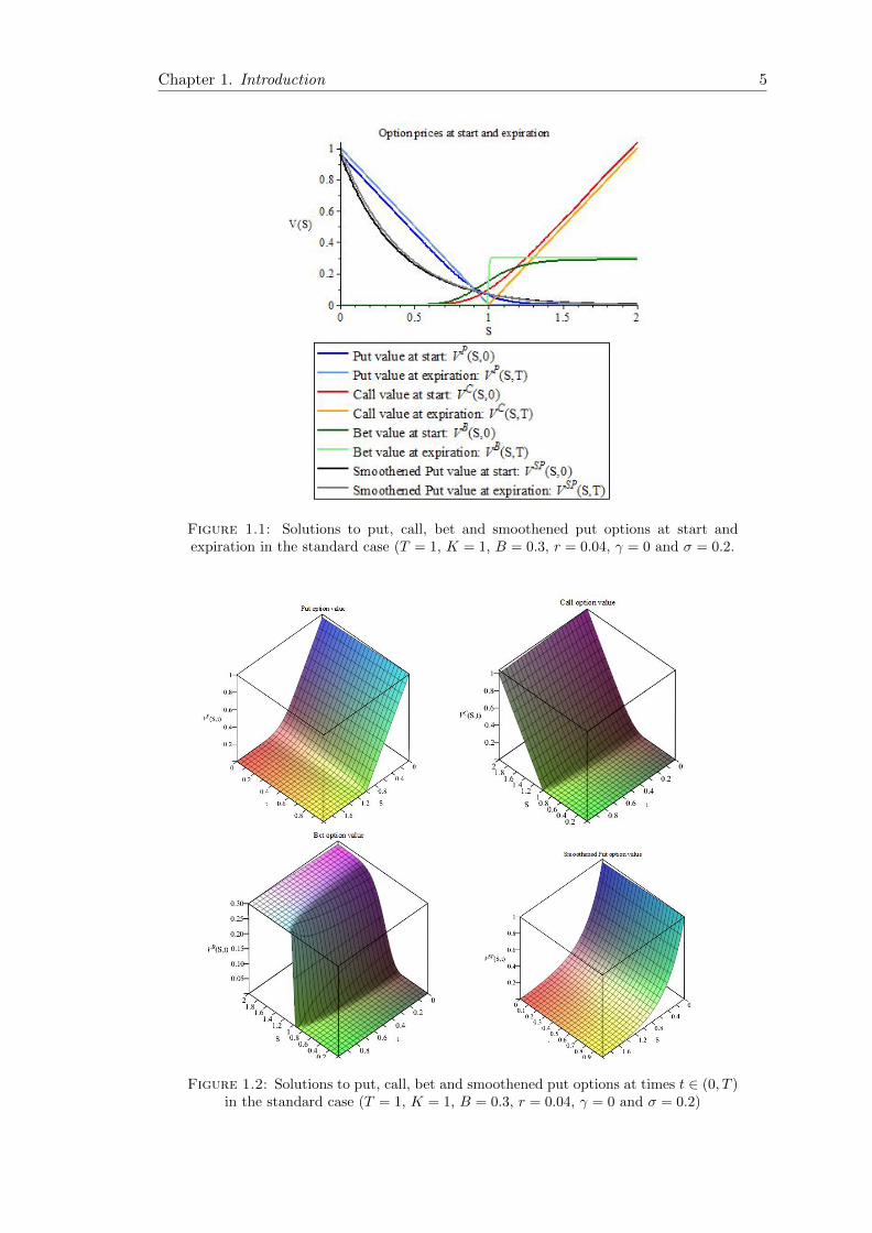
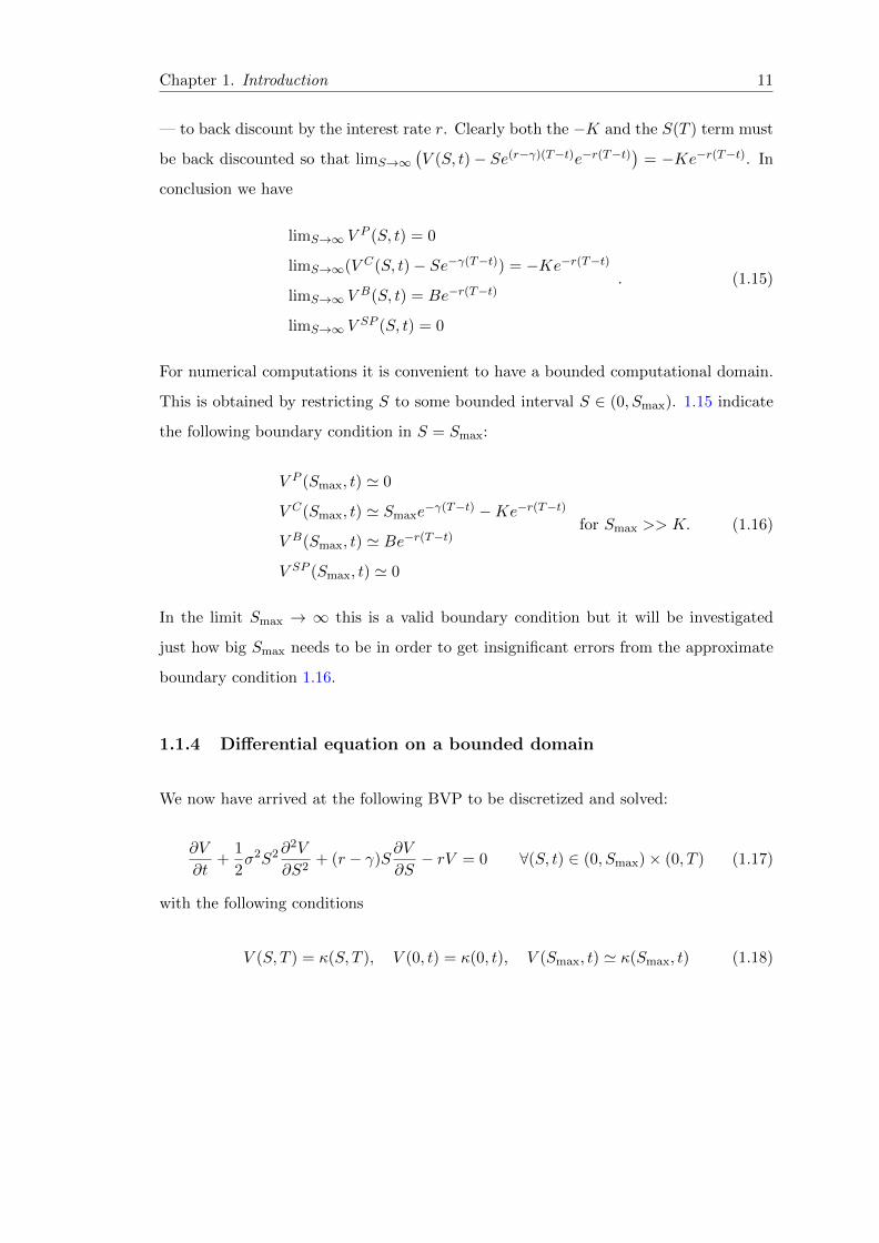
2D solution plots for the standard case at start (t = 0) and expiration (t = T ) are shown
in Figure 1.1. Corresponding 3D solution plots showing solutions for all time values
t ∈ (0, T ) are shown in Figure 1.2.
From V the Deltas given by ∆ = ∂V∂S can be computed. Only ∆P and ∆C are “challeng-
ing”, but these are well known from for example [46] §5.4 (for γ = 0) or [20] §1.3.1 (for
Chapter 1. Introduction 5
Figure 1.1: Solutions to put, call, bet and smoothened put options at start andexpiration in the standard case (T = 1, K = 1, B = 0.3, r = 0.04, γ = 0 and σ = 0.2.
Figure 1.2: Solutions to put, call, bet and smoothened put options at times t ∈ (0, T )in the standard case (T = 1, K = 1, B = 0.3, r = 0.04, γ = 0 and σ = 0.2)

Chapter 1. Introduction 6
all cases):
∆P (S, t) =∂V P
∂S(S, t) = eγ(T−t)(N(d1)− 1), (1.5)
∆C(S, t) =∂V C
∂S(S, t) = eγ(T−t)N(d1), (1.6)
∆B(S, t) =∂V B
∂S(S, t) = Be−r(T−t)n(d2), (1.7)
where n(d) =∂N(d)
∂Sso that
n(d1) =e−
12d2
1
√2πSσ
√T − t
and n(d2) =e−
12d2
2
√2πSσ
√T − t
.
2D Delta plots for the standard case at start (t = 0) and expiration (t = T ) are shown
in Figure 1.3. Corresponding 3D Delta plots showing Delta values for all time values
Figure 1.3: Deltas for put, call, bet and smoothened put options at start and expira-tion in the standard case (T = 1, K = 1, B = 0.3, r = 0.04, γ = 0 and σ = 0.2)
t ∈ (0, T ) are shown in Figure 1.4.
From V the Gammas given by Γ = ∂2V∂S2 can be computed:
ΓP (S, t) =∂2V P
∂S2(S, t) = eγ(T−t)n(d1), (1.8)
ΓC(S, t) =∂2V C
∂S2(S, t) = eγ(T−t)n(d1), (1.9)
ΓB(S, t) =∂2V B
∂S2(S, t) = −Be−r(T−t)n(d2)
S
(d2
σ√T − t
+ 1
). (1.10)

Chapter 1. Introduction 7
Figure 1.4: Deltas for put, call, bet and smoothened put options at times t ∈ (0, T )in the standard case (T = 1, K = 1, B = 0.3, r = 0.04, γ = 0 and σ = 0.2)
2D Gamma plots for the standard case at start (t = 0) and expiration (t = T ) are shown
in Figure 1.5. Corresponding 3D Delta plots showing Gamma values for all time values
Figure 1.5: Gammas for put, call, bet and smoothened put options at start andexpiration in the standard case (T = 1, K = 1, B = 0.3, r = 0.04, γ = 0 and σ = 0.2)
- The put and call Gammas are identical

Chapter 1. Introduction 8
in (0, T ) are shown in Figure 1.6.
Figure 1.6: Gammas for put, call, bet and smoothened put options at times t ∈ (0, T )in the standard case (T = 1, K = 1, B = 0.3, r = 0.04, γ = 0 and σ = 0.2)
For particular parameter selections, the solution, ∆ and Γ of the smoothened put op-
tion can be computed for example using the Finance package of the Maple symbolic
computation environment. The solutions, ∆’s and Γ’s are shown in Figures 1.1–1.6.

Chapter 1. Introduction 9
1.1.3 Limits
There are some interesting limits to the problem 1.1:
Volatility limit: For σ = 0 the option loses its stochastic aspect and behaves like a
riskfree asset with the payoff function as the terminal value at time T and dividend γ
in a world with interest rate r. The value at time t is then the amount of money that,
if put in the bank at interest rate r would result in the same value of payoff at time T
as if holding the option. But this amount is simply the terminal value back discounted
by r so that V (S, t)|σ=0 = V (S(T ), T )e−r(T−t). Here S(T ) is the value of the (now
risk-free) risky asset at expiration t = T . To express it by S we simply back discount
it by r − γ since we could get the interest rate r by selling the stock and putting the
money in the bank, but at the same time we would then lose the dividend rate γ. Hence
S = S(T )e−(r−γ)(T−t). In conclusion
V (S, t)|σ=0 = V (Se(r−γ)(T−t), T )e−r(T−t) (1.11)
As σ → 0, the convection-diffusion equation loses its diffusion part and becomes a
convection equation. Hence it is not known whether
limσ↓0
V (S, t) = V (S, t)|σ=0 (1.12)
but it will be investigated whether the numerical solutions have this desirable property.
Expiration limit: For t = T the option price is given by the payoff function V (S, T ).
Even though V B(S, T ) is discontinuous and V C(S, T ) and V P (S, T ) have discontinuous
first derivatives the formulas for the exact solutions show that these singularities are
instantaneously smoothened out for t < T or τ > 0 and also that
limt↑T
V (S, t) = V (S, T ). (1.13)
Enforcing V (S, T ) as a terminal boundary condition and solving backwards in time, also
a numerical solution will have this desirable property, but it will be investigated whether
the discontinuities as expected give rise to problems in the numerical solution.

Chapter 1. Introduction 10
Left risky asset limit: For S = 0 the risky asset has lost all value corresponding
to Bankruptcy. If bankruptcy happens at a time t∗, then (see note 2 in [23]) S(t)
remains zero for t ≥ t∗. Hence the option has lost its stochastic aspect and behaves
like a riskfree asset with interest rate r. Hence the value is simply the terminal value
V (S(T ), T ) = V (0, T ) back discounted by r so that
V P (0, t) = Ke−r(T−t)
V C(0, t) = 0
V B(0, t) = 0
V SP (0, t) = Ke−r(T−t)
. (1.14)
This condition may (and will) be enforced as a boundary condition to the differential
equation 1.1. Note that this is not entirely unquestionable since the PDE 1.1 in the limit
S → 0 loses all dependence on S. Hence a boundary condition in S = 0 may actually
give rise to problems for a numerical solution.
Right risky asset limit: For S → ∞ the limiting behavior is again determined by
certainty, i.e. lack of stochastic uncertainty. If we are certain to get a payback M at time
T then the value at t ∈ (0, T ) is as above the r-backdiscounted value of M , Me−r(T−t).
For a put option with large S >> K at some time t ∈ (0, T ) we are almost certain to end
up at time T with the payback 0. As S is increasing, the certainty grows, and in the limit
S →∞ the certainty becomes total resulting in limS→∞ VP (S, t) = 0. The smoothened
put will be given the same right boundary condition as the ordinary put. Similarly for
a bet option with large S >> K at some time t ∈ (0, T ) we are almost certain to end up
at time T with the payback B. As S is increasing, the certainty grows, and in the limit
S → ∞ the certainty becomes total resulting in limS→∞ VB(S, t) = Be−r(T−t). For a
call option with large S >> K at some time t ∈ (0, T ) we are almost certain to end up
at time T with the payback S(T ) −K. As S is increasing, the certainty grows, and in
the limit S → ∞ the certainty becomes total. The problem is, that S(T ) is stochastic
so that the payoff is not certain. Considering instead a portfolio consisting of one call
option and minus one risky asset then the payoff at time T on this portfolio is certain to
be −K in the limit as S →∞. Hence limS→∞ (V (S(T ), T )− S(T )) = −K. To express
the terminal risky asset price S(T ) by the asset price S at time t we follow the argument
from the volatility limit and get limS→∞(V (S(T ), T )− Se(r−γ)(T−t)) = −K. To express
also the option price in terms of S and t we need — as explained for the volatility limit
Chapter 1. Introduction 11
— to back discount by the interest rate r. Clearly both the −K and the S(T ) term must
be back discounted so that limS→∞(V (S, t)− Se(r−γ)(T−t)e−r(T−t)
)= −Ke−r(T−t). In
conclusion we have
limS→∞ VP (S, t) = 0
limS→∞(V C(S, t)− Se−γ(T−t)) = −Ke−r(T−t)
limS→∞ VB(S, t) = Be−r(T−t)
limS→∞ VSP (S, t) = 0
. (1.15)
For numerical computations it is convenient to have a bounded computational domain.
This is obtained by restricting S to some bounded interval S ∈ (0, Smax). 1.15 indicate
the following boundary condition in S = Smax:
V P (Smax, t) ' 0
V C(Smax, t) ' Smaxe−γ(T−t) −Ke−r(T−t)
V B(Smax, t) ' Be−r(T−t)
V SP (Smax, t) ' 0
for Smax >> K. (1.16)
In the limit Smax → ∞ this is a valid boundary condition but it will be investigated
just how big Smax needs to be in order to get insignificant errors from the approximate
boundary condition 1.16.
1.1.4 Differential equation on a bounded domain
We now have arrived at the following BVP to be discretized and solved:
∂V
∂t+
1
2σ2S2∂
2V
∂S2+ (r − γ)S
∂V
∂S− rV = 0 ∀(S, t) ∈ (0, Smax)× (0, T ) (1.17)
with the following conditions
V (S, T ) = κ(S, T ), V (0, t) = κ(0, t), V (Smax, t) ' κ(Smax, t) (1.18)

Chapter 1. Introduction 12
where function κ(S, t) is defined as follow
κ(S, t) =
maxSe−γ(T−t) −Ke−r(T−t), 0 call option
maxKe−r(T−t) − Se−γ(T−t), 0 put option
Be−r(T−t)H(S −K) bet option
K Smax−SSmax
e−2S−r(T−t) smoothened put
. (1.19)
1.1.5 Transformations of differential equation
By the simple change of variables
τ = T − t ∀t ∈ [0, T ], i.e. ∀τ ∈ [0, T ] (1.20)
1.17–1.19 is transformed into the following initial value problem:
Find U : (S, τ) ∈ Ω→ R where Ω = (0, Smax)× (0, T )
for some Smax >> K,
so that in a classical, weak or distributional sense
−∂U∂τ
+1
2σ2S2∂
2U
∂S2+ (r − γ)S
∂U
∂S− rU = 0 in Ω and (1.21)
U(S, 0) = κ(S, T ), U(0, τ) = κ(0, τ), U(Smax, τ) ' κ(Smax, τ)
where the connection between 1.17 and 1.21 is that
U(S, τ) = V (S, T − t), ∀(S, t) ∈ Ω i.e. ∀(S, τ) ∈ Ω. (1.22)
The two formulations are equivalent, and we shall stick to the former, without losing
generality. At any point it is easy to change to forward notation, simply changing from
time t to reverse time τ as shown above.
Another common transformation of 1.17 is determined by
τ =1
2σ2(T − t) ∀t ∈ [0, T ], i.e. ∀τ ∈ [0, T ].
x = ln
(S
K
)∀S ∈ [0, Smax], i.e. ∀x ∈ [−∞, xmax], where
xmax = ln
(Smax
K
). (1.23)

Chapter 1. Introduction 13
1.17 is then transformed into the following initial value problem:
Find W : (x, τ) ∈ Ωln → R where Ωln = (−∞, xmax)× (0, T )
for some xmax >> 0,
so that in a classical, weak or distributional sense
∂W
∂τ=∂2W
∂x2in Ωln and (1.24)
W (−∞, τ) =
e−(β+ r
12σ
2)τ
put or smoothened put option
0 call option
0 bet option
,
W (xmax, τ) '
0 put or smoothened put option
e−αxmax−βτ(SmaxK e
− γ12σ
2τ− e− r
12σ
2τ)
call option
BK e−αxmax−(β+ r
12σ
2)τ
bet option
W (x, 0) =
e−αx max(1− ex, 0) put option
e−αx max(ex − 1, 0) call option BK e−αx for K(ex − 1) ≥ 0
0 for K(ex − 1) < 0bet option
1K e−αx(1− ex−xmax)e−2Kex smoothened put option
,
where the connection between 1.17 and 1.24 is that
V (S, t) = Keαx+βτW (x, τ), ∀(S, t) ∈ Ω∞ i.e. ∀(x, τ) ∈ Ωln
α =1
2
(1− r − γ
12σ
2
), β = −1
4
(1− r − γ
12σ
2
)2
− r12σ
2(1.25)
and where it is assumed that α < 0 in order to avoid problems at x = −∞. The two
formulations are equivalent, and while we shall stick to the former, we shall utilize known
results from the second (the heat equation).
1.1.6 Numerical methods for solving European option on bounded do-
main
Some numerical methods for solving the option price model on the bounded domain are
the following standard text book finite difference schemes:

Chapter 1. Introduction 14
a. Forward or explicit Euler: Forward2 in time t, central in S [FtCS]. Error and
stability condition for the heat equation: O(k + h2) and k ≤ h2
2 respectively.
b. Backward or implicit Euler: Backward in time t, central in S [FtCS]. Error and
stability condition for the heat equation: O(k + h2) and A- and L-stable respec-
tively.
c. Crank Nicolson: Central in time t, central in S [FtCS]. Error and stability condi-
tion for the heat equation: O(k2 + h2) and A- but not L-stable respectively.
d. Lax Friedrich: Error and stability condition for the heat equation: O(h2 + k+ h2
k )
and k ≤ h respectively.
e. Leapfrog: Error and stability condition for the heat equation: O(k2 + h2) and
unconditionally unstable respectively.
f. DuFort-Frankel: Error and stability condition for the heat equation: O(h2 + k2 +
k2
h2 ) and A- but not L-stable respectively.
All these methods are consistent3 except for the DuFort-Frankel method which is only
conditionally consistent.
The numerical schemes are constructed on a net of nodal points (Sn, tm), n = 1, . . . , N ,
m = 1, . . . ,M with step sizes h and k respectively, so that Sn = (n−1)h and tm = (M−
m)k and in particular S1 = 0, SN = Smax, t1 = T and tM = 0. Then the schemes consist
of simple replacements [;] in 1.17-1.19: The Dirichlet terminal and boundary conditions
are used as they are: V (0, tm) ; V1,m = V (0, tm), V (Smax, tm) ; VN,m = V (Smax, tm),
V (Sn, T ) ; Vn,1 = V (Sn, T ) for n = 1, . . . , N and m = 1, . . . ,M . The derivatives
DV (Sn, tm) in the relevant (mainly interior) nodal points in 1.17-1.19 are replaced by
2 Note that since we solve a backward DEP, The timesteps in Forward Euler is actually taking usbackwards in time, and similarly for the other noncentral methods.
3The finite difference schemes converge to the DEP as the stepsizes go to 0.

Chapter 1. Introduction 15
finite differences δVn,m varying from method to method:
Find Vn,m for n = 1, . . . , N and m = 1, . . . ,M :
δtVn,m +1
2σ2S2
nδSSVn,m + (r − γ)SnδSVn,m − rδ0Vn,m = 0
for n = 2, . . . , N − 1 and m = 1, . . . ,M − 1, (M − 2 for Leapfrog and DuFort-Frankel),
V1,m = κ(0, tm), for m = 1, . . . ,M,
VN,m ' κ(Smax, tm), for m = 1, . . . ,M,
Vn,1 = κ(Sn, T ) for n = 1, . . . , N, (1.26)
For the various finite difference schemes we have the following replacements:
a. Forward Euler:
V (Sn, tm) ; δ0Vn,m = Vn,m,
∂V∂t (Sn, tm) ; δtVn,m =
Vn,m+1−Vn,mk ,
∂V∂S (Sn, tm) ; δSVn,m =
Vn+1,m−Vn−1,m
2h ,
∂2V∂S2 (Sn, tm) ; δSSVn,m =
Vn+1,m−2Vn,m+Vn−1,m
h2 ,
for n = 2, . . . , N − 1, m = 1, . . . ,M − 1.
b. Backward Euler:
V (Sn, tm+1) ; δ0Vn,m = Vn,m+1,
∂V∂t (Sn, tm+1) ; δtVn,m =
Vn,m+1−Vn,mk ,
∂V∂S (Sn, tm+1) ; δSVn,m =
Vn+1,m+1−Vn−1,m+1
2h ,
∂2V∂S2 (Sn, tm+1) ; δSSVn,m =
Vn+1,m+1−2Vn,m+1+Vn−1,m+1
h2 ,
for n = 2, . . . , N − 1, m = 1, . . . ,M − 1.
c. Crank Nicolson:
V (Sn, tm+ 12) ; δ0Vn,m = 1
2
(Vn,m+1 + Vn,m
),
∂V∂t (Sn, tm+ 1
2) ; δtVn,m =
Vn,m+1−Vn,mk ,
∂V∂S (Sn, tm+ 1
2) ; δSVn,m = 1
2
(Vn+1,m+1−Vn−1,m+1
2h +Vn+1,m−Vn−1,m
2h
),
∂2V∂S2 (Sn, tm+ 1
2) ; δSSVn,m = 1
2
(Vn+1,m+1−2Vn,m+1+Vn−1,m+1
h2 +Vn+1,m−2Vn,m+Vn−1,m
h2
),
for n = 2, . . . , N − 1, m = 1, . . . ,M − 1.
d. Lax Friedrich:
V (Sn, tm) ; δ0Vn,m = Vn,m,
∂V∂t (Sn, tm) ; δtVn,m =
Vn,m+1−Vn,mk + h2
2kVn+1,m−2Vn,m+Vn−1,m
h2 ,

Chapter 1. Introduction 16
∂V∂S (Sn, tm) ; δSVn,m =
Vn+1,m−Vn−1,m
2h ,
∂2V∂S2 (Sn, tm) ; δSSVn,m =
Vn+1,m−2Vn,m+Vn−1,m
h2 ,
for n = 2, . . . , N − 1, m = 1, . . . ,M − 1.
e. Leapfrog:
V (Sn, tm+1) ; δ0Vn,m = Vn,m+1,
∂V∂t (Sn, tm+1) ; δtVn,m =
Vn,m+2−Vn,m2k ,
∂V∂S (Sn, tm+1) ; δSVn,m =
Vn+1,m+1−Vn−1,m+1
2h ,
∂2V∂S2 (Sn, tm+1) ; δSSVn,m =
Vn+1,m+1−2Vn,m+1+Vn−1,m+1
h2 ,
for n = 2, . . . , N − 1, m = 1, . . . ,M − 2.
f. DuFort-Frankel:
V (Sn, tm+1) ; δ0Vn,m = Vn,m+1,
∂V∂t (Sn, tm+1) ; δtVn,m =
Vn,m+2−Vn,m2k + k2
h2Vn,m+2−2Vn,m+1+Vn,m
k2 ,
∂V∂S (Sn, tm+1) ; δSVn,m =
Vn+1,m+1−Vn−1,m+1
2h ,
∂2V∂S2 (Sn, tm+1) ; δSSVn,m =
Vn+1,m+1−2Vn,m+1+Vn−1,m+1
h2 ,
for n = 2, . . . , N − 1, m = 1, . . . ,M − 2.
1.2 Nonlinear Black-Scholes Models
The standard Black-Scholes equation is supposed in a complete market under some
simplified assumptions such as liquid market with no transaction cost. Taking into
account one or some of theses parameters to have more reliable option price causes a
nonlinear Black-Scholes equation with a nonlinear volatility function. In Chapters 4-5
nonlinear Black-Scholes equations have been considered with nonlinear volatility that
depends on time t, underlying asset price S and the second derivative of option price
V (S, t) with respect to S. Also several schemes have been applied and compared to solve
the nonlinear Black-Scholes models in these two chapters. Here we review a number of
nonlinear volatility models. Note that in these models σ0 (the volatility of the underlying
asset) is assumed constant and if we take σ(t, S, VSS) = σ0 we will have the classical
linear Black-Scholes model.

Chapter 1. Introduction 17
1.2.1 Leland Model
The models that we have grouped together here are all addressing the issue of nonzero
transaction cost assumed to be a fixed fraction of the volume of transactions. The
original paper [30] takes
σ2L(t, S, VSS) = σ2
0
[1 + Le× sign
(∂2V
∂S2
)](1.27)
for a call option, where Le is the Leland number given by
Le =
√2
π
κ
σ0
√δt.
κ denotes the round trip transaction cost per unit dollar of transaction and δt is the
transaction frequency (interval between successive revisions of the portfolio). There was
an error in the Leland argument, but it was apparently not published until 2003 in [47].
Some years before that Boyle and Vorst [6] modified the Leland number, replacing the
factor√
2/π ' 0.8 by 2, and showed using the binomial model that if the transaction
frequency δt - taken equal to the time step in the binomial model - and the transaction
cost κ tend to zero (while keeping the ratio κ√δt
of the order one) then the discrete option
price converges to the Black-Scholes price for a call option with a modified volatility of
the form
σ2(t, S, VSS) = σ20
[1 +
2κ
σ0
√δt× sign
(∂2V
∂S2
)].
For both of the above volatility models, the parameters κ and δt should be given so that
σ2(t, S, VSS) > 0. Two years later Hoggard et al [21] derived the following nonlinear
volatility model for a call option:
σ2(t, S, VSS) = σ20
[1−
√2
π
2κ
σ0
√δt× sign
(∂2V
∂S2
)]
including the negative of the product of the Leland factor√
2π and the Boyle and Vorst
factor 2. For a short position in a call option both Boyle and Vorst and Hoggard et al
changes the sign on the modified Leland number, thus still having opposite signs. The
Hoggard et al volatility model is known as the HWW transaction cost model.

Chapter 1. Introduction 18
1.2.2 Risk Adjusted Pricing Methodology(RAPM)
The RAPM model was introduced by Kratka in 1998 [27] as an attempt to include
effects of transaction cost as well as risk from volatile portfolios into the Black-Scholes
model. Jandacka and Sevcovic [25] later criticized the Kratka method for not being
mathematically well-posed and scale invariant and presented the following alternative
version:
σ2JS(t, S, VSS) = σ2
0
[1 + µ(S
∂2V
∂S2)
13
](1.28)
where µ = 3(κ2R2π
) 13. κ ≥ 0 (denoted C in [25]) is the transaction cost from the Leland
model and the risk premium coefficient R ≥ 0 represents the marginal value of the in-
vestor’s exposure to risk. More precisely, the change in the portfolio value arising from
risk from the volatility of the portfolio per unit asset price and per unit time ( ∆ΠS∆t) is
modelled by RVar(∆Π/S)∆t , Var being the variance. Jandacka and Sevcovic model [25]
solves the nonlinear Black-Scholes problem by first deriving a quasilinear parabolic PDE
for H = S ∂2V∂S2 and solving this with a semi-implicit in time finite difference scheme and
then plugging the numerical values of H into the exact solution for the standard Black-
Scholes problem with constant volatility and integrating numerically using a trapezoidal
quadrature. Kutik and Mikula [28] proposed a Crank-Nicolson-type scheme for the solu-
tion of the quasilinear H-equation from Jandacka and Sevcovic model [25] and compared
it to the semi-implicit scheme in that paper. They found 2nd order convergence of the
Crank-Nicolson scheme against linear convergence of the semi-implicit scheme.
1.2.3 Barles and Soner model
As for the RAPM, Barles and Soner [4] considers both transaction cost and risk from
volatile portfolios. They start commenting on the Leland number that the size of the
constant√
2π is really irrelevant for the argument and may be replaced by any constant
c without changing the argument thus basically validating all the different Leland con-
stants in use. Then a different approach based on utility maximization is introduced
Chapter 1. Introduction 19
resulting in the following adjustment of the volatility:
σ2BS(t, S, VSS) = σ2
0
[1 + Ψ
(er(T−t)κ2RS2∂
2V
∂S2
)](1.29)
where κ is the Leland transaction cost (denoted µ in [4]) and R is a risk aversion factor
(denoted γ in [4]) and probably similar to the risk premium coefficient in Jandacka and
Sevcovic model [25]. Finally Ψ(x) is the solution of the nonlinear ODE
Ψ′(x) =Ψ(x) + 1
2√xΨ(x)− x
, x 6= 0 (1.30)
with the initial condition Ψ(0) = 0. In appendix A of [4] the existence of a unique
continuous viscosity solution to this problem has been shown. It is also shown that
σ2BS ≥ 0 i.e. that the adjustment factor to σ2
0 is nonnegative for any argument of Ψ. For
the numerical experiments an unspecified explicit time stepping finite difference scheme
is used with small time steps near maturity (t = T ) and larger time steps away from
maturity. Lesmana and Wang [31] present numerical results for the Barles and Soner
model using instead an implicit first order time stepping and upwind asset price stepping
finite difference method.
1.2.4 Feedback and illiquid market
Frey et al [16, 14, 15] do not consider transaction cost but look at the effects of assuming
that the asset price depends on the hedging strategy (feedback) applied in an illiquid
market with dynamic hedging. They argue for the nonlinear volatility model
σ2FP (t, S, VSS) =
σ20(
1− ρλ(S)S ∂2V∂S2
)2 (1.31)
where ρ > 0 is a constant and λ(S) > 1 is a strictly convex function. For numerical
computations they put in cut-off’s to prevent σFP → 0 and σFP →∞:
σ2FP (t, S, VSS) = σ2
0 maxα0,1(
1−minα1, ρλ(S)S ∂2V∂S2
)2 (1.32)

Chapter 1. Introduction 20
where α0 = 0.02 and α1 = 0.85. Liu and Yong [32] continue the work on the Frey model
but addresses also transaction cost. Frey’s ρ factor is absorbed into the λ function and
an expression for this function is given resulting in the model
σ2LY (t, S, VSS) =
σ20(
1− λ(S, t)S ∂2V∂S2
)2 (1.33)
where λ(S, t) is given by
λ(S, t) =
γS (1− e−β(T−t)) for 0 ≤ S ≤ Smax
0 otherwise
where γ > 0 measures the price impact per traded share and is given the value 0.04 in the
article. β is given the value 100 in the article. Liu and Yong [32] have also established
sufficient conditions for existence and uniqueness of the solution of this generalized
Black-Scholes equation.
1.2.5 Parameterized Illiquidity Model
Bakstein and Howison [3] develop a parameterized model for illiquidity effects arising
from the discrete trading in an asset with transaction costs. Liquidity is defined via a
combination of a trader’s individual transaction cost and a price slippage impact, which
is felt by all market participants:
σ2BH(t, S, VSS) = σ2
0
[1 + 2λS
∂2V
∂S2+
(λµS
∂2V
∂S2
)2
+
(κµ
σ0
√δt
)2
+ 2
√2
π
κ
σ0
√δt
sign
(∂2V
∂S2
)+ 2
√2
πλµ2 κ
σ0
√δtS
∣∣∣∣∂2V
∂S2
∣∣∣∣](1.34)
where λ > 0 models the market depth, which represents the elasticity of the asset price
to the quantity traded and µ > 0 models the slippage measure that transforms the
average transaction price into the next published price. Finally κ and δt are the Leland
transaction cost (denoted γ in the article) and transaction frequency. Bakstein and
Howison [3] present a model according to which the parameters are observable from
order-book data, rather than having to be estimated from market data.

Chapter 1. Introduction 21
In Chapter 4 we consider the feedback and illiquid market (1.2.4) and solve this model
with Forward Euler, Backward Euler and Crank Nicolson schemes and also investigate
how choosing the right boundary (Smax) can effect on option price and numerical error
[24]. We investigate the Barles and Soner model (1.2.3) in Chapter 5. We consider some
different finite difference schemes Forward Euler, Positive preserving, Crank Nicolson,
Implicit Upwind and nonstandard finite difference mmethod for this nonlinear model
and present some comparisons of the schemes and some numerical experiments.


Chapter 2
Kα-Shifting, Rannacher Time
Stepping and Mesh Grading in
Crank Nicolson FDM for
Black-Scholes Option Pricing
Sima Mashayekhi and Jens Hugger
Abstract. Non-smooth conditions in partial differential equations cause discretization
error in numerical schemes and lead to decay in the convergence rate. Here the Kα-
shifting method is introduced for easy handling of uniform and nonuniform meshes and
for one or more singularities in the terminal condition. Combining this method with
Rannacher time stepping and mesh grading for the Crank-Nicolson Finite Difference
Method on some examples including call options, bet options and a butterfly spread is
shown to lead to higher accuracy and better convergence rate for the numerical solution.
Keywords: Black-Scholes model; Rannacher time stepping; finite difference schemes;
Crank-Nicolson scheme; European options
Subjectclass: 65M06; 65M12; 65N06; 65N12
23

Chapter 2. Kα, Rannacher and mesh grading in CN for B-S option pricing 24
2.1 Introduction
We consider the well established Black-Scholes model for the pricing of a few standard
European vanilla options on a bounded domain:
∂V
∂t+
1
2σ2S2∂
2V
∂S2+ (r − γ)S
∂V
∂S− rV = 0 ∀(S, t) ∈ (0, Smax)× (0, T ) (2.1)
with the terminal and boundary conditions
V (S, T ) = κ(S, T ), V (0, t) = κ(0, t), V (Smax, t) ' κ(Smax, t) (2.2)
where we are using the utility function
κ(S, t) =
maxSe−γ(T−t) −Ke−r(T−t), 0 call option
maxKe−r(T−t) − Se−γ(T−t), 0 put option
Be−r(T−t)H(S −K) bet option
max(K + a)e−r(T−t) − Se−γ(T−t), 0H(S −K)
+ maxSe−γ(T−t) − (K − a)e−r(T−t), 0H(K − S) butterfly spread
(2.3)
V (S, t) is the (fair) option price for a value S of the risky asset at time t. r, σ and γ
are the market interest rate (on a risk free asset), the volatility (of the underlying risky
asset) and the dividend yield (on the risky asset) respectively. Smax >> K is the upper
bound for the computational domain in the S variable and the terminal time T is the
upper bound in the t variable. K is the Strike Price for the call and put, B the value of
the Bet and a is the distance from the strike prices K±a of the long options to the strike
price K of the two short options in the butterfly spread. H is the Heaviside function.
In this article we provide numerical solutions using the standard Crank-Nicolson (CN)
Finite Difference Method (FDM) with a few simple adaptations. Further we compute
the Greeks Delta (∆(S, t) = ∂V∂S (S, t)) and Gamma (Γ(S, t) = ∂2V
∂S2 (S, t)) using second
order finite differences, centered in the interior points and one sided at the boundaries.
These methods are easy to program and account for the majority of the PDE-methods
in use today. The main underlying concept is that we would like to consider simple
(if possible a priori) modifications to the in practice most commonly used methods in
order to show how to improve results of these methods by simple adjustments without
abandoning the methods.

Chapter 2. Kα, Rannacher and mesh grading in CN for B-S option pricing 25
(a) e(S, t) for call. (b) e(S, t) for bet. (c) e(S, t) for butterfly spread.
Figure 2.1: Plot of the error e(S, t) as function of S ∈ (0, Smax) and t ∈ (0, T ) for (a)call option, (b) bet option and (c) butterfly spread with Smax ' 4K in the standardcase (T = 1, K = 1, a = 0.2, B = 0.3, r = 0.04, γ = 0, σ = 0.2 and Smax = 4K) with
the Crank-Nicolson (CN) method for a mesh with h = 0.08 and k = 0.01.
FDM’s only provide results in grid points of the finite difference subdivisions. Results
in other points are obtained by simple interpolation, typically linear but also higher
order interpolations may be used if higher degree of precision is required. This is an
issue if a value (or Greek) at a discontinuity is requested. If the discontinuity is a nodal
point, derivatives must be defined with care and if not the interpolation in the point
must be defined with care. We shall not require singularities to be nodal points since
this as we shall show may result in increased error. Instead we refer to interpolation
for such values. Using the Finite Element Method (including in the term all projection
based methods finding solutions in a finite dimensional subspace of a sufficiently smooth
function space) interpolation issues do not exist, but we shall not consider such methods
here, as they are still not very common in practice, in particular not methods with
enough smoothness to recover for example the Gamma (∂2V∂S2 ) since the Black-Scholes
equation naturally leads to weak solutions in H1 only offering a continuous solution V
and one weak derivative (∂V∂S ).
The discontinuities in the terminal condition or its first derivative seen in (2.2) lead
to decay in the convergence rate of most finite difference numerical schemes for “com-
putable” stepsizes h in the S-variable and k in the t-variable, see for example [46, 44].
This happens also for the Crank-Nicolson (CN) method which is the one that we shall
focus on in this article. Typical plots of the error e (CN solution minus exact solu-
tion in the nodal points) for call, bet and butterfly spread are shown in Figure 2.1,
where the dominating error concentrated around the singularity S = K or singularities

Chapter 2. Kα, Rannacher and mesh grading in CN for B-S option pricing 26
S = K,K ± a respectively is notable. The goal of this work is to investigate how the
“size of the bump(s)” can be reduced without abandoning the CN method.
Rannacher [39] introduced a start-up procedure for Crank-Nicolson in which one or more
initial time steps are replaced by small implicit Euler time steps in order to achieve the
expected second order convergence in the follow up Crank-Nicolson method since the
order of the standard Crank-Nicolson scheme may be reduced all the way down to zero
in the case of rough terminal data. This approach, commonly known as Rannacher time
stepping, is widely adopted in financial engineering practice and hence will be considered
among the simple modifications allowed in this article.
Another approach, see [44, 38], addresses the decay in convergence order by considering
the position of the strike price K with respect to the grid points used in the method. It is
shown that having K in the middle between two nodal points in a finite difference scheme
decreases the oscillations around the strike price when compared to having K located in
a nodal point and consequently increases the accuracy of the finite difference method.
Pooley et al [38] consider another alternative for reducing error from nonsmooth terminal
conditions, namely smoothening of the terminal data either by a simple averaging over
half of the cells to the left and right of the nodal point or by a projection (an L2 projection
is suggested) onto a set of continuous piecewise linear Finite Element basis functions.
While the repositioning of a singular point can be performed a priori and hence can be
implemented in any existing code at very low cost, the smoothening methods require
reconstructing a code and thus falls outside the goal of this article to consider only
simple adjustments easily applicable to existing code. Instead they are highly relevant
when we in the future extend our work to finite element methods (see section 2.5).
It is also well known (see for example [40, 37]), that an alternative to Rannacher timestep-
ping is nonuniform (exponentially increasing) time steps (or equivalently a square root of
time variable change). Such methods show good promises even for singularities as strong
as the Dirac delta function and hence can be used also for at least some Greeks. The
method requires either a transformation of the problem or schemes accepting nonuni-
form time steps and hence falls outside the scope of this article and is relegated to future
work (see section 2.5).
In this article we introduce a shifting grid points method (Kα-shifting) which puts the
strike price at any preselected position between nodal points. In section 2.2 we explain

Chapter 2. Kα, Rannacher and mesh grading in CN for B-S option pricing 27
in more details the Kα-shifting method for uniform and nonuniforn meshes with one or
more singularities in the terminal value and show its effect for some numerical examples.
Moreover we consider stability of the optimal choice of Kα with respect to different
parameters in the Black-Scholes equation.
In section 2.3 we compare Crank-Nicolson with and without the Kα-shifting method
and with and without Rannacher time stepping. We give results for uniform as well as
nonuniform graded meshes.
In section 2.4 we compare the orders of convergence of these four methods for option
prices and the Greeks ∆ and Γ.
Finally some concluding remarks and possible future work is discussed in section 2.5.
2.2 Kα-shifting
The Kα-shifting method addresses the significance of the location of singular points in
the terminal condition in relation to the end points of the S-elements. We consider
“reasonable” parameter values T = 1, K = 1, a = 0.2, B = 0.3, r = 0.04, γ = 0, σ = 0.2
and Smax = 4K (denoted the standard case) and solve the call, bet and butterfly spread.
(The put option is omitted since the put-call-parity makes it somewhat superfluous).
For the put, call and bet options the single singularity occurs in S = K whereas for the
butterfly spread there are 3 singularities in K − a, K and K + a.
Consider first the case of uniform meshes with step sizes h in the S-variable and k in the
t-variable and the case of one singularity in S = K. First the mesh interval containing
K (controlled by ıK) and the relative position of K in this interval (controlled by α) are
found from
Find ıK , α : K − Smin = (ıK + α)h for some ıK ∈ N and 0 ≤ α < 1, (2.4)
where Smin denotes the left endpoint of the computational S-domain which is 0 in our
case, but may be 6= 0 in the generalizations of the Kα-shifting method below. Then h
is adjusted to h using
Find iK , h : K − Smin = (iK +Kα)h for some iK ∈ N : ıK ≤ iK ≤ ıK + 1. (2.5)

Chapter 2. Kα, Rannacher and mesh grading in CN for B-S option pricing 28
iK is given by
iK =
⌈K − Smin
h−Kα
⌉=
⌈K − Smin
h− α+ (α−Kα)
⌉= dıK + (α−Kα)e
= ıK + dα−Kαe ∈ [ıK , ıK + 1], (2.6)
and hence
K − Smin = (
⌈K − Smin
h−Kα
⌉+Kα)h⇔ h =
K − Smin⌈K−Smin
h−Kα
⌉+Kα
. (2.7)
Note that the new S step size h is given by a simple updating formula from the known
input parameters h and Kα without actually ever computing ıK and α. Also h is close
to h since
ıKh ≤ iKh ≤ K − Smin ≤ (ıK + 1)h
and (ıK + 2)h ≥ (iK + 1)h ≥ K − Smin ≥ ıK h
⇓ıK
ıK + 2h ≤ h ≤ ıK + 1
ıKh. (2.8)
For very coarse meshes the adjustment of the S step size may be substantial, like hh∈
[0.83, 1.1] for K situated in the 10’th interval (ıK = 10) but for more realistic meshes,
the adjustment is minimal, like hh∈ [0.98, 1.01] for K situated in the 100’th interval
(ıK = 100).
Two further adjustment must be made, that are not part of the Kα-shifting method, but
are necessary in order to adjust S = Smax (the user requested maximal S value in the
computational domain) and t = 0 to be nodal points. First Smax is adjusted (increased)
to Smax lying in the nodal point (in the S-variable) closest to but at least as big as Smax
using
Smax − Smin =
⌈Smax − Smin
h
⌉h ≥ Smax − Smin. (2.9)
Finally k is adjusted (reduced) to k so that t = 0 is a nodal point (in the t-variable)
using
k =T⌈Tk
⌉ ≤ k and T −⌈T
k
⌉k = 0 where
⌈T
k
⌉∈ N . (2.10)

Chapter 2. Kα, Rannacher and mesh grading in CN for B-S option pricing 29
These adjustments (h → h, Smax → Smax and k → k) are simple update formulas and
hence cheap (O(1)) that do not deteriorate the performance of the solution process and
can be performed a priory and hence used with any existing code. They may result
in slightly fluctuating errors when the requested step sizes are large and hence also the
adjustments are potentially large. For “reasonable” step sizes however the results of the
adjustments are negligible. Instead with the Kα-shifting method there are no fluctuation
in the error caused by K “moving around” inside the iK ’th interval when adjusting the
mesh interval size. This turns out to be a significant advantage in practical use, since
the error from K moving around is significant (up to a factor of more than 10 for the
maximal error).
The Kα-shifting method for uniform meshes easily generalizes to more than one singu-
larity. Just divide the S domain into patches each containing one of the singularities.
For each patch — starting from the left with the patch containing S = 0 — compute the
adjusted step size and adjust the right endpoint of the patch to be a nodal point with
the adjusted step size. In (2.4)–(2.9) just use the left patch endpoint as Smin, the right
endpoint of the patch as Smax and the adjusted right endpoint of the patch as Smax.
For small requested stepsize h all the actual stepsizes will be very close in size, so that
even uniform finite difference approximations will give good results in particular because
patch boundaries are situated in areas where the computed solution is almost linear, but
otherwise nonuniform finite differences across the patch boundaries may be used. The
only issue is that for more than one singularity the method cannot be performed entirely
a priory since it requires the ability to work with slightly different stepsizes in different
parts of the domain and preferably also with nonuniform finite difference approximations
across the patch boundaries, which a standard uniform mesh code will not be able to
handle.
For nonuniform meshes constructed by a grading function the idea would be the following
for a single singularity in S = K: If K is contained in the element number [SiK , SiK+1[
then simply relocate this element without resizing it to say [S0, S1[ so that K moves into
Kα-position in the element. This relocation is then followed by a uniform scaling of the
rest of the elements. The global scaling factors sK− and sK+ for the elements before
and after K respectively are given by
sK− =S0 − Smin
SiK − Smin, sK+ =
Smax − S1
Smax − SiK+1, (2.11)

Chapter 2. Kα, Rannacher and mesh grading in CN for B-S option pricing 30
so that the size of all elements before K are multiplied by sK− and the size of all
elements after K are multiplied by sK+. A simpler alternative would be simply to use
the Kα-shifting method for uniform meshes on the uniform mesh being graded. For small
elements the grading function will be sufficiently close to linear to put the singularity
close enough to the Kα-position.
For adaptively constructed nonuniform meshes with one singularity in S = K the idea
would be very similar to the first one for the grading function approach: If the element
[SıK , SıK+1[ containing K in Kα-position is up for subdivision — let us for simplic-
ity say uniform splitting into two equal elements — then the new elements are con-
structed, and the new element [SiK , SiK+1[ containing K (either [SıK ,SıK+SıK+1
2 [ or
[SıK+SıK+1
2 , SıK+1[) is relocated (but not resized), say to [S0, S1[ so that K is again in
Kα-position in this element. This relocation is followed by global scalings of the elements
to the left and right as for the grading function approach, using the scaling factors sK−
and sK+ defined in (2.11).
If finally N > 1 singularities are present with nonuniform meshes then N patches each
containing exactly one singularity are constructed and each patch is scaled with indi-
vidual scaling factors moving from the left to the right. If the nonuniform meshes are
created with a grading function, the simple approach also generalizes. Just use the Kα-
shifting method for uniform meshes with several singularities explained above on the
uniform mesh being graded.
Turning to the computational examples, instead of using h, k and Smax we shall use
the notation h ' . . ., k ' . . . and Smax ' . . . to account for the adjustments. For given
values of all parameters we compute maximal absolute solution errors at time t = 0 over
all S nodal points S1, . . . , SM as
E0V = max
i=1...,M|VFDM (Si, 0)− V BS(Si, 0)| (2.12)
where VFDM (Si, 0) is the computed finite difference solution in the nodal point S =
Si and t = 0 and V BS(Si, 0) is the exact (Black-Scholes) solution in the same point.
Similarly we define the maximal absolute errors E0∆ and E0
Γ for the Greeks ∆ and Γ.
In Figure 2.2 we show the maximal absolute solution errors E0V (Kα) at time t = 0 for
two different sets of step sizes (h, k) ' (0.08, 0.01) and (h, k) ' (0.03, 0.001) and as a

Chapter 2. Kα, Rannacher and mesh grading in CN for B-S option pricing 31
(a) E0V (Kα) for call with the coarse mesh. (b) E0
V (Kα) for call with the fine mesh.
(c) E0V (Kα) for bet with the coarse mesh. (d) E0
V (Kα) for bet with the fine mesh.
Figure 2.2: Maximal error E0V (Kα) at time t = 0 as function of Kα ∈ [0, 1] for call
and bet options in the standard case solved with CN using the coarse mesh (h, k) '(0.08, 0.01) and the fine mesh (h, k) ' (0.03, 0.001).
function of 41 different Kα-values uniformly distributed from 0 to 1 for the call and
the bet option solution values. When Kα = 0 or 1 (or whenever S = K is a nodal
point) it becomes a numerical issue how to define V (K,T ) for the bet option. After
some experimentation we have decided to use the convention V (K,T ) = 0 for Kα < 0.5
and V (K,T ) = B for Kα ≥ 0.5 giving the smoothest graphs. We are interested in Kα,
the optimal Kα, minimizing E0V over all values of Kα ∈ [0, 1[. Kα = 0.27 turns out to
be the optimal choice for the call option at time t = 0 (see Figures 2.2(a) and 2.2(b))
varying from 0.280 for the coarse mesh to 0.264 for the fine mesh when computed with
1001 uniformly distributed Kα-values from 0 to 1. Also we observe that the symmetric

Chapter 2. Kα, Rannacher and mesh grading in CN for B-S option pricing 32
position Kα = 1−0.27 is quite good, and actually the entire interval (0.2, 0.8) gives good
results (at most the double maximal absolute solution error compared to the optimal
location). The general conclusion is that for the call option (and similarly for the put)
the strike price K should under no circumstances be located close to a nodal point.
Figures 2.2(c) and 2.2(d) show that Kα = 0.50 is the optimal choice for the bet option
at time t = 0, varying from 0.508 for the coarse mesh to 0.504 for the fine mesh when
computed with 1001 Kα-values. Unsurprisingly Kα = 0.50 is optimal also when solving
with graded meshes. Hence the best location for the strike price is in the middle between
two consecutive nodal points. The interval where the maximal error is at most the double
of the optimal error is (0.4, 0.6) and hence significantly smaller for the bet option than for
the call. Also the price for locating the strike price closer to a nodal point is significantly
bigger for the bet than for the call option. The general conclusion is that for the bet
option the strike price K should under no circumstances be located close to a nodal
point.
Figure 2.3 shows the maximal absolute errors at time t = 0 for the Greeks ∆ and Γ for
the call and bet options with the fine mesh (h, k) ' (0.03, 0.001) and for 41 different Kα-
values uniformly distributed from 0 to 1. Computing with 1001 uniformly distributed
Kα-values from 0 to 1 we get the following optimal Kα-values: For the call option
Kα = 0.00 and Kα = 0.33 for the Delta and Gamma respectively. Note however, that
the value of Kα is of little importance for the Greeks of the call option, all minimal
errors lying within a factor significantly below 2 from the smallest value. For the bet
option Kα = 0.51 and Kα = 0.53 for the Delta and Gamma respectively. For the bet
option the value of Kα is important also for the Greeks, the factor two interval being
as small as [0.48, 0.58]. Concluding, for the bet option Kα = 0.5 is the sensible choice
for both the value, the Delta and the Gamma, whereas for the call Kα should be picked
in the interval [0.2, 0.8] and might be picked at Kα = 0.5 without an increase of more
than a factor 2 in the maximal error for the value, the Delta and the Gamma. The
small irregularities visible in Figures 2.2–2.3 (for the coarse mesh solution of the call
at Kα ' 0.5 and for the fine mesh solutions of the call Greeks at Kα ' 0.35) originate
from various numerical “issues” related to the computation of either numerical or exact
values. Since the irregularities do not influence the conclusions we have not investigated
the exact causes in each case.

Chapter 2. Kα, Rannacher and mesh grading in CN for B-S option pricing 33
(a) E0∆(Kα) for call with the fine mesh. (b) E0
Γ(Kα) for call with the fine mesh.
(c) E0∆(Kα) for bet with the fine mesh. (d) E0
Γ(Kα) for bet with the fine mesh.
Figure 2.3: Maximal error E0∆(Kα) and E0
Γ(Kα) at time t = 0 for the Greeks ∆ andΓ for the call and bet options as function of Kα ∈ [0, 1] in the standard case solved
with CN using the fine mesh (h, k) ' (0.03, 0.001).
The butterfly spread requires 3 optimal Kα-values denoted K1α, K2
α and K3α for the
singularities K − a, K and K + a respectively. The corresponding 3 patches are chosen
a priori as [0,K − a2 ], [K − a
2 ,K + a2 ] and [K + a
2 , Smax] and then adjusted by the
Kα-shifting method. For different values of N we have computed with N each of K1α-
, K2α- and K3
α-values uniformly distributed in [0, 1] for a total of N3 cases. Also we
have computed for the coarse as well as for the fine mesh as defined above. Given
the 3-dimensional parameter space (K1α,K
2α,K
3α) ∈ [0, 1]3 visualization of the results is
somewhat challenging, so here we only show the results in tabular form in Table 2.1.
For comparison we have also in Table 2.1 given the errors for the two most likely cases

Chapter 2. Kα, Rannacher and mesh grading in CN for B-S option pricing 34
Table 2.1: Optimal Kα-values for solution, ∆ and Γ for the butterfly spread in thestandard case solved with CN using the coarse mesh (h, k) ' (0.08, 0.01) and the fine
mesh (h, k) ' (0.03, 0.001).
Mesh No. Kα’s K1α K2
α K3α minKα E
0V (Kα)
maxKα E0V (Kα)
minKα E0V (Kα)
1 0.00 0.00 0.00 0.016762 11 0.50 0.50 0.50 0.009338 1
Coarse V 113 0.50 0.33 0.33 0.000765 34.928762213 0.55 0.30 0.20 0.000622 46.712522413 0.53 0.28 0.18 0.000595 49.446807
1 0.00 0.00 0.00 0.004325 11 0.50 0.50 0.50 0.001495 1
Fine V 113 0.60 0.50 0.40 0.000105 93.523044213 0.60 0.50 0.40 0.000105 93.523044413 0.50 0.38 0.25 0.000091 −a
1 0.00 0.00 0.00 0.114845 11 0.50 0.50 0.50 0.039337 1
Coarse ∆ 113 0.40 0.00 0.60 0.008357 29.840102213 0.45 0.05 0.65 0.008320 30.770937413 0.38 0.00 0.65 0.007997 34.449918
1 0.00 0.00 0.00 0.020239 11 0.50 0.50 0.50 0.006166 1
Fine ∆ 113 0.20 0.00 0.80 0.001466 24.887289213 0.30 0.10 0.85 0.001354 26.942537413 0.28 0.08 0.85 0.001333 −a
1 0.00 0.00 0.00 0.385213 11 0.50 0.50 0.50 0.186919 1
Coarse Γ 113 0.40 0.10 0.90 0.116449 6.817861213 0.40 0.10 0.85 0.108821 7.503789413 0.40 0.10 0.85 0.108821 7.848675
1 0.00 0.00 0.00 0.086126 11 0.50 0.50 0.50 0.030656 1
Fine Γ 113 0.50 0.30 0.00 0.017846 6.569529213 0.55 0.35 0.05 0.017247 7.348245413 0.53 0.35 0.10 0.016665 −a
aOnly selected subintervals of Kα are computed.
Kα = [0, 0, 0] which would likely occur if no thought is given to the location of the
singularities (typically integer multiple of decimal steplengths) and Kα = [0.5, 0.5, 0.5]
which would likely occur if it was decided to put the singularities in a fixed position
different from nodal points without considering optimality of the position. First of all
the results show that Kα-optimization gives a significant reduction with a factor from
5 to 30 in the error in the solution, ∆ and Γ when compared to selecting Kα = [0, 0, 0].
When compared to Kα = [0.5, 0.5, 0.5] we still record a significant reduction in the error

Chapter 2. Kα, Rannacher and mesh grading in CN for B-S option pricing 35
with an improvement of more than a factor 10 for the solution, less but still with a factor
of about 5 for the ∆ and least but still with a factor of around 2 for the Γ. This confirms
our previous results that the Kα-optimization is less important for the Greeks than for
the solution. For Γ basically any selection of Kα apart from putting the singularities in
(or close to) nodal points is good.
All the results of this section indicate that positioning the strike price near the middle
of a mesh interval might be a good although conservative approach giving reasonable
results for many options. If looking for the very best the positioning of the strike price
must be taking into consideration also the type of option.
For the Kα-optimization to be useful in practice it would need to be fairly stable against
variations in the parameters. So next we investigate whether the conclusions depend on
the particular selection of model parameters above. Here interest rate r and volatility
σ are deemed the most important parameters, whereas T , B and K basically can be
considered scaling parameters without much significance and the dividend yield γ is
expected to behave like some sort of additional interest rate, a constant γ not creating
new features by itself. Hence in the following two subsections we shall consider variations
of the optimal Kα with interest rate r and volatility σ respectively.
2.2.1 Stability of Kα with respect to the interest rate
We redo the computations from Figure 2.2 only adding a third axis with the interest rate
r ∈ [−0.1, 0.1]. Negative interest rates are considered since interest rates in Europe has
fallen very close to zero after the financial crisis in 2010 and there has been discussions of
whether negative interest rates were necessary in order to spawn investment in “growth”
i.e. in risky assets.
Two typical results for the fine mesh are shown in Figure 2.4 where we have computed
with equidistant r-values with the same difference 0.025 as is used for the Kα-values.
For the call option the optimal Kα is situated in (0.2, 0.3) ∪ (0.7, 0.8). Further a Kα in
the extended interval (0.2, 0.8) only changes the minimal error for the call option by a
factor of up to 2 whereas a Kα outside this interval may change the minimal error for
the call option by a factor of up to 4.

Chapter 2. Kα, Rannacher and mesh grading in CN for B-S option pricing 36
(a) E0V (Kα, r) for call with the fine mesh. (b) E0
V (Kα, r) for bet with the fine mesh.
Figure 2.4: Maximal error E0V (Kα, r) at time t = 0 as function of Kα ∈ [0, 1] and
r ∈ [−0.1, 0.1] for (a) the call and (b) the bet option in the standard case except for rsolved with CN using the fine mesh (h, k) ' (0.03, 0.001).
For the bet option the optimal Kα is situated in (0.45, 0.55) and any Kα in this interval
only changes the minimal error for the bet option by a factor of up to 2 whereas a Kα
outside this interval may change the minimal error for the bet option by a factor of up
to 10.
Summing up, the conclusions from section 2.2 hold for all values of r and t. A reasonable
conservative choice is to pick Kα = 0.5, but for the call option a more refined choice
would be to select Kα = 0.725 for negative interest rates and 0.275 for positive interest
rates. Especially for the bet option a selection of Kα = 0 is somewhat disastrous and
should be avoided whether by choice or accident.
2.2.2 Stability of Kα with respect to the volatility
We redo the computations from Figure 2.2 this time adding a third axis with the volatility
σ ∈ (0.1, 0.4). Two results are shown in Figure 2.5. The conclusions are the same as
before: For the call option the optimal Kα shift for some σ-values from a “lower” value
close to the 0.275 observed typically for small values of σ to an “upper” value close to the
symmetric value 0.725 = 1− 0.275 observed typically for large values of σ. The optimal
Kα is situated in (0.1, 0.3) ∪ (0.7, 0.9). Further a Kα in the extended interval (0.1, 0.9)
only changes the minimal error for the call option by a factor of up to 2 whereas a Kα
outside this interval may change the minimal error for the call option by a factor of up
to 4.

Chapter 2. Kα, Rannacher and mesh grading in CN for B-S option pricing 37
(a) E0V (Kα, σ) for call with the fine mesh. (b) E0
V (Kα, σ) for bet with the fine mesh.
Figure 2.5: Maximal error E0V (Kα, σ) at time t = 0 as function of Kα ∈ [0, 1] and
σ ∈ [0.1, 0.4] for (a) the call and (b) the bet option in the standard case except for σsolved with CN using the fine mesh (h, k) ' (0.03, 0.001).
The optimal Kα for the bet option is still located solidly in 0.5 except for a few cases
with small σ, and for Kα ∈ (0.4, 0.6) the maximal error is at most the double of the
minimal value of the maximal error, whereas a Kα outside this interval may change the
minimal error for the bet option by a factor of up to 10.
Summing up, the conclusions from section 2.2 hold for all values of σ and r. A reasonable
conservative choice is to pick Kα = 0.5, but for the call option a more refined choice
would be to select Kα = 0.725 for large volatilities and 0.275 for small volatilities.
Especially for the bet option a selection of Kα = 0 is somewhat disastrous and should
be avoided whether by choice or accident.
2.3 Kα-shifting, Rannacher time stepping and mesh grad-
ing
Recall Figure 2.1 showing the CN error as a function of S ∈ (0, Smax) and t ∈ (0, T ). In
this section we focus on reducing the size of the “bump” in the error close to S = K for
all values of t ∈ (0, T ). As in section 2.2 we consider the 2D-slice t = 0 but limit to the
bet option with its larger error and hence bigger room for improvement than the call
option. We shall investigate the error in the Greeks ∆ and Γ as well as the error in the
solution and compare the base results for the standard CN method to results obtained
with CN with a Rannacher startup phase [CNR], CN with the optimal Kα [CNKα] and

Chapter 2. Kα, Rannacher and mesh grading in CN for B-S option pricing 38
a new combination of CN with both a Rannacher startup phase as well as the optimal
Kα [CNRKα]. We compute with a uniform mesh but for the solution errors we also
show results computed with a nonuniform mesh (method suffix GS for Grid Stretching,
eg. CNGS) created with the mesh grading transformation
S(x) = K +1
bsinh(c1(1− x) + c2x) with
c1 = arc sinh(−bK)
c2 = arc sinh(b(Smax −K))(2.13)
changing a uniform mesh in x ∈ [0, 1] with stepsize dx into a nonuniform mesh in
S ∈ [0, Smax] (See more details in Appendix 2.A). The grading of the S-mesh depends
on the grading parameter b which we take to b = 15 (see [44, 36, 43]). The maximal
absolute solution error (see (2.12)) with nonuniform meshes is denoted E0V,nu.
We consider the Rannacher method in the form where the first iteration of the Crank-
Nicolson method is replaced by four quarter-timesteps of the implicit Euler scheme. Giles
et al [17] have shown that four quarter-timesteps of the implicit Euler method replacing
the first CN step is more accurate than replacing the first two CN steps by four half-
timesteps of implicit Euler due to a reduction of the low wavenumber error introduced
by the Rannacher startup. Giles et al do so using an x = logS transformation of the
S-variable and no transformation of the time variable giving a reasonable expectation
that the conclusion will hold also without the transformation of the S-variable which we
shall not apply here. Moreover Giles et al have shown that choosing λ? = kσh√
2T∈ [0.5, 1]
causes maximum accuracy for a given computational cost. This result is not expected
to carry over to our case but keeping λ∗ the same as in the Giles et al paper gives a good
basis for comparison since logS is almost linear in the most interesting region around
S = K = 1.
For comparison we consider the same parameter values as chosen by Giles et al [17]:
T = 2, K = 1, B = 0.3, r = 0.05, γ = 0, σ = 0.2 and Smax ' 5K (denoted the
Giles case). Also we take λ? = 0.5 corresponding to k = 5h and h = 0.01. (For the
nonuniform meshes dx = 0.01/Smax to get the same number of elements in S). While h
and k are not disclosed in [17], it is evident from [17, Fig. 1-2] that also they do consider
the worst possible case (Kα = 0). In Figures 2.6–2.9 we show the solution, Delta and
Gamma errors at time t = 0 for the bet option with CN, CNR, CNKα and CNRKα.

Chapter 2. Kα, Rannacher and mesh grading in CN for B-S option pricing 39
(a) enu(S, 0) for bet with CNGS. (b) enu(S, 0) for bet with CNRGS.
(c) enu(S, 0) for bet with CNKαGS. (d) enu(S, 0) for bet with CNRKαGS.
Figure 2.6: Solution error enu(S, 0) at time t = 0 as function of S ∈ (0, Smax)with a mesh graded by (2.13) with b = 15 for the bet option in the Giles case withdx = 0.01/Smax and k = 0.05 solved with (a) CNGS with Kα = 0, (b) CNRGS with
Kα = 0, (c) CNKαGS with Kα = 0.5 and (d) CNRKαGS with Kα = 0.5.
In Table 2.2 the maximal errors of the various cases considered in Figures 2.6–2.9 are
listed.
The results show two features: A high frequency oscillation and a “bump” both occurring
near S = K. For the standard CN method the oscillations are fairly small compared
to the bump for the solution error, sizable for the ∆ error and all dominating for the
Γ error. Rannacher startup completely removes the oscillations for the solution and ∆
error and very significantly reduces the oscillations for the Γ. Instead Rannacher startup
does nothing to reduce the “bump”. The Kα method reduces the size of the “bump”

Chapter 2. Kα, Rannacher and mesh grading in CN for B-S option pricing 40
(a) e(S, 0) for bet with CN. (b) e(S, 0) for bet with CNR.
(c) e(S, 0) for bet with CNKα. (d) e(S, 0) for bet with CNRKα.
Figure 2.7: Solution error e(S, 0) at time t = 0 as function of S ∈ (0, Smax) for thebet option in the Giles case with h = 0.01 and k = 5h solved with (a) CN with Kα = 0,
(b) CNR with Kα = 0, (c) CNKα with Kα = 0.5 and (d) CNRKα with Kα = 0.5.
but does not remove the oscillation like the Rannacher startup. Finally it is seen how
adding the Kα-optimization together with the Rannacher startup completely removes
the oscillatory part of the solution and ∆ error and significantly reduces it for the Γ
error. On top of this the size of the bump is significantly reduced for both solution,
∆ and Γ error. For the total error for the CNRKα-method, including oscillation and
bump, the maximal solution error is reduced by a factor of 100 with respect to the CNR
solution error. This factor reduces to 44 for the Delta error and 10 for the Gamma
error, but in all cases the reduction is at least an order of magnitude. These factors
are computed from Table 2.2. It should be noted that our results for CN and CNR are

Chapter 2. Kα, Rannacher and mesh grading in CN for B-S option pricing 41
(a) e∆(S, 0) for bet with CN. (b) e∆(S, 0) for bet with CNR.
(c) e∆(S, 0) for bet with CNKα. (d) e∆(S, 0) for bet with CNRKα.
Figure 2.8: Delta error e∆(S, 0) at time t = 0 as function of S ∈ (0, Smax) for the betoption in the Giles case with h = 0.01 and k = 5h solved with CN with Kα = 0 (a),
CNR with Kα = 0 (b), CNKα with Kα = 0.5 (c) and CNRKα with Kα = 0.5 (d).
completely consistent with those of [17, Fig. 2].
After establishing the merit of the CNRKα-method for the bet option for one mesh, we
turn to the question of whether this is just a very particular case? So we solve for both
the call and the bet option with a number of different values of h ∈ [0.002, 0.1] in the
Giles case. Also we again take λ? = 0.5 corresponding to k = 5h. For the Kα-shifting
methods we use Kα = 0.275 for the call option and Kα = 0.5 for the bet option. For
the non Kα-shifting methods actually we take Kα = 0 to show some sort of “worst case
scenario”. For the “true” non Kα-shifting methods, the error will fluctuate erratically

Chapter 2. Kα, Rannacher and mesh grading in CN for B-S option pricing 42
(a) eΓ(S, 0) for bet with CN. (b) eΓ(S, 0) for bet with CNR.
(c) eΓ(S, 0) for bet with CNKα. (d) eΓ(S, 0) for bet with CNRKα.
Figure 2.9: Gamma error eΓ(S, 0) at time t = 0 as function of S ∈ (0, Smax) for thebet option in the Giles case with h = 0.01 and k = 5h solved with (a) CN with Kα = 0,
(b) CNR with Kα = 0, (c) CNKα with Kα = 0.5 and (d) CNRKα with Kα = 0.5.
Table 2.2: The maximal solution, Delta and Gamma errors over S ∈ (0, Smax) at timet = 0 for the bet option in the Giles case with h = 0.01 and k = 5h (dx = 0.01/Smax,for E0
V,nu) solved with CN with Kα = 0, CNR with Kα = 0, CNKα with Kα = 0.5 andCNRKα with Kα = 0.5
Methods E0V,nu E0
V E0∆ E0
Γ
CN 0.113659 0.00255428 0.0258461 24.9258CNR 9.11740e-05 0.00191539 0.00580019 0.0303068CNKα 0.113888 0.000743987 0.0268447 27.4361CNRKα 5.48878e-06 1.71763e-05 0.000132096 0.00298739

Chapter 2. Kα, Rannacher and mesh grading in CN for B-S option pricing 43
between this worst case scenario curve and the curve for the optimal Kα depending on
whether the actual Kα is far from or close to optimal.
Apart from uniform meshes we also compute for nonuniform meshes created with the
mesh grading function (2.13) indicated with a [GS] for grid stretching after the acronym
for the method. As above, for the nonuniform meshes we take dx = h/Smax to get the
same number of elements in S and k = 5h. In order to visualize the wide intervals of
h-values and corresponding maximal errors we show the results on double logarithmic
scales. Instead of showing plots of the errors for all values of S ∈ (0, Smax) at t = 0 as
we did in Figures 2.6–2.9 we now only show maximal errors over S ∈ (0, Smax) at t = 0
in Figure 2.10.
It is seen, that Rannacher time stepping is essential in order to obtain convergence
and for all cases Rannacher time stepping combined with mesh grading decreases the
error although not the order of convergence. Rannacher time stepping combined with
Kα-optimization is clearly the better choice when it comes to order of convergence
and combining also with mesh grading decreases the error further without increasing
the order of convergence. Hence only the CNRKα- and CNRKαGS-methods can be
recommended for general use. The CN, CNR and CNKα-methods (with or without
mesh grading) must be considered unsuited for general use even though of course they
can be used in particular cases especially if only limited precision is required. The
conclusion is, that the CNRKαGS-method is the overall winner as a general method for
computing solution, Delta and Gamma values for put, call and bet options.
Our results for the call option in the left column of Figure 2.10 for CN and CNR are
very similar in structure to those of Giles et al [see 17, Fig. 3]. In reality, the Giles et al
results more resemble our results for CNKα and CNRKα. For the bet option shown in
the right column of Figure 2.10 it is even more clear, that it is our results for CNKα and
CNRKα that are comparable with the Giles et al results for CN and CNR [see 17, Fig.
4]. A personal communication with Mike Giles reveals that Giles et al [17] as a matter
of fact consistently did use stepsizes putting the strike either in a nodal point [see 17,
Fig. 1-2] or in the middle of a mesh interval [see 17, Fig. 3-4].

Chapter 2. Kα, Rannacher and mesh grading in CN for B-S option pricing 44
(a) Call maximal error. (b) Bet maximal error.
(c) Delta call maximal error. (d) Delta bet maximal error.
(e) Gamma call maximal error. (f) Gamma bet maximal error.
Figure 2.10: Maximal solution (a)-(b), ∆ (c)-(d) and Γ (e)-(f) errors at time t = 0as function of h ∈ (0.002, 0.1) for the call option with Kα = 0.275 for the Kα methodsand Kα = 0 for the non Kα methods (left column) and bet option with Kα = 0.500 forthe Kα methods and Kα = 0 for the non Kα methods (right column) in the Giles casewith k = 5h and dx = h/Smax for graded meshes. Each plot is showing error curvesE0V , E0
∆ or E0Γ respectively for uniform meshes for the 4 methods CN, CNR, CNKα
and CNRKα and error curves E0V,nu, E0
∆,nu or E0Γ,nu respectively for graded meshes for
the 4 methods CNGS, CNRGS, CNKαGS and CNRKαGS.

Chapter 2. Kα, Rannacher and mesh grading in CN for B-S option pricing 45
2.4 Order of Convergence
For problems without degenerations and singularities the maximal error with the Crank-
Nicolson method should converge to zero as O(h2) + O(k2) but the singular terminal
conditions are known to decrease the orders of convergence for “computable” step sizes.
The loss of convergence order is bigger the worse the singularity is and hence we focus
on the bet option showing results for the error in the solution, the ∆ and the Γ, the
latter having the strongest singularity.
Figure 2.11 shows the maximal solution errors at time t = 0 for the bet option with
logarithmic axes. The results are provided for the Giles case with h ∈ (2−8, 2−3) and
k ∈ (10−0.2, 10−1.7). For the CN and CNKα methods the (h, k)-plane is clearly divided
into two regions with different behavior of the error: In one part a reduction in k reduces
the error whereas a reduction in h increases the error. This part will be denoted the
bubble. The rest of the (h, k)-plane is denoted the asymptotic part. The CNR and
CNRKα methods show no bubble part, only the asymptotic part. In order to estimate
convergence orders in both h and k independently we use a weighted least squares fitting
of the computational errors E0V of the form
mina,b,α,β
∑i,j
wi,j · ((E0V )i,j − (a · hαi + b · kβj ))2. (2.14)
The stepsizes are recorded so that they decrease with increasing index, i.e. hi+1 ≤ hi
and kj+1 ≤ kj , and the simple weight function wi,j = i · j putting higher weight on
smaller step sizes is applied. Obviously selecting a different weight function may change
the results somewhat. Separate fittings are made for the bubble and asymptotic parts.
In the least squares minimizations the side conditions 0 ≤ a, 0 ≤ b, 0 ≤ α ≤ 3 and
0 ≤ β ≤ 3 are imposed. In a few cases β > 2. In these cases β is restricted to 0 ≤ β ≤ 2
and the least squares fitting is repeated. If the maximal fitting error is not increased on
the leading digit, then the latter result is selected. The following convergence orders are

Chapter 2. Kα, Rannacher and mesh grading in CN for B-S option pricing 46
(a) E0V for bet with CN. (b) E0
V for bet with CNR.
(c) E0V for bet with CNKα. (d) E0
V for bet with CNRKα.
Figure 2.11: Maximal error E0V over S ∈ (0, Smax) at time t = 0 as function of the
step sizes h = dS and k = dt for the bet option in the Giles case for (a) CN (Kα = 0),(b) CNR (Kα = 0), (c) CNKα (Kα = 0.5) and (d) CNRKα (Kα = 0.5)
computed for the error in the bet option:
E0V [CN ] '
0.5 · k0.5 bubble
0.7 · h1.1 + 0.002 asymptotic
E0V [CNR] ' 0.7 · h1.0 + 0.001 · k0.5
asymptotic
E0V [CNKα] '
0.6 · k0.7 bubble
0.4 · h1.9 asymptotic
E0V [CNRKα] ' 0.4 · h1.9 + 0.005 · k2.0
asymptotic (2.15)
Similar computations are performed for the Delta and Gamma errors of the bet option

Chapter 2. Kα, Rannacher and mesh grading in CN for B-S option pricing 47
but the convergence plots look very similar in structure to Figure 2.11 and are not shown
here. Instead the approximate convergence results are given. The Delta errors for the
bet option are computed as
E0∆[CN ] '
77 · k0.7 bubble
1.0 · h0.8 asymptotic
E0∆[CNR] ' 1.1 · h0.9 + 0.06 · k2.0
asymptotic
E0∆[CNKα] '
77 · k0.7 bubble
3.6 · h1.9 asymptotic
E0∆[CNRKα] ' 3.7 · h1.9 + 0.004 · k2.0
asymptotic (2.16)
and the Gamma errors for the bet option are computed as
E0Γ[CN ] '
36000 · k0.3 bubble
8.0 · h0.9 + 0.9 · k2.0 asymptotic
E0Γ[CNR] ' 7.9 · h1.0 + 1.0 · k1.2
asymptotic
E0Γ[CNKα] '
35000 · k0.3 bubble
18.3 · h1.7 + 1.6 · k2.0 asymptotic
E0Γ[CNRKα] ' 17.0 · h1.7 + 0.03 · k0.9
asymptotic (2.17)
We see evidence that the CN and CNR methods are missing one order of convergence in
h i.e. in the S-direction. The convergence in k i.e. in the t-direction is quite imprecise.
Because of the small coefficient the term is only visible for large values of k where the
results are maybe not even in the asymptotic range. The CNKα and CNRKα methods
reestablishes (almost) full quadratic convergence in h (1.9 for solution and ∆ errors and
1.7 for Γ error). The convergence in k is also for these methods “problematic”, but
somewhat better than for the methods without Kα optimization.
Similar calculations for the call option results in the same conclusion only with a more
perfect recovery of the optimal results since the singularity for the call option is weaker
than for the bet option. Hence again, the CNRKα method must be the one recommended
for general use.

Chapter 2. Kα, Rannacher and mesh grading in CN for B-S option pricing 48
2.5 Conclusions and future work
We investigated the Crank-Nicolson finite difference method [CN] and simple improve-
ments for European vanilla options (put, call, bet and butterfly spread).
We proposed the Kα method for uniform and nonuniform meshes with one or more
singularities in the terminal condition and tested it with good results for uniform and
graded meshes with 1 or 3 singularities.
We found that the Rannacher start up method removes high frequency oscillations in
the CN-solution, Delta and Gamma error around the “bump” in the maximal error (see
Figure 2.1) and partially reestablishes the optimal second order convergence in the t-
direction of the CN method. Instead it does not decrease the size of the error bump or
improve the order of convergence in the S-direction.
The Kα method instead reduces the size of the bump in the CN-error and partially
reestablishes the optimal second order convergence in the S-direction of the CN method.
Instead it does not remove the high frequency oscillations around the bump or improve
the order of convergence in the t-direction.
The CN method with the addition of both the Rannacher and the Kα method re-
moves the high frequency oscillations around the maximal error in the solution, Delta
and Gamma and significantly reduces the size of the error bump. Further it partially
reestablishes the optimal second order convergence in the S and t-direction of the CN
method.
Finally we found that mesh grading further reduces the maximal error in all methods
without changing orders of convergence thus establishing the merit of utilizing nonuni-
form meshes in the S-variable.
The Rannacher and Kα methods can be included into any finite difference scheme with
very low cost, and is expected to give similar improvements as for the Crank-Nicolson
method.
We have also shown that the optimal Kα-values depend on the option but that they
are almost independent of the parameters (in particular of the interest r, the volatility
σ and the step sizes h and k). For the call option the optimal Kα lies in (0.2, 0.3) or
(0.7, 0.8) for the solution error but the error is not very sensitive to values of Kα in

Chapter 2. Kα, Rannacher and mesh grading in CN for B-S option pricing 49
(0.2, 0.8). Values outside this interval may instead lead to significant increases in the
error. For the ∆ and Γ errors for the call the choice of Kα is almost insignificant but
does have an optimal value at Kα = 0 (and 1) and 0.3 respectively. For the bet option
the optimal Kα is 0.5 for the solution, ∆ as well as the Γ error and should be picked in
(0.45, 0.55). Values outside this interval may lead to significant increases in the error.
For possible future work we are planning to apply Kα-shifting to nonuniform S-grids
considering both graded meshes and adaptive meshes. We intend to do this for finite
difference grids, but also to extend to the finite element method, where theoretical results
are more easily obtained.
Also we will apply Kα-shifting to problems without closed form solutions such as Amer-
ican options, Asian options, basket options, options with variable parameters (such as σ
and γ) and options from a generalized Black-Scholes world taking into consideration for
example nonvanishing trading cost, influence from trading volume on stock prices and
other features leading to “nonlinear volatility” options.


Appendix
2.A Grid Stretching
The grid stretching transformation concentrates nodal points around non-smooth points
of initial conditions for instance the strike price for European options and leads decreas-
ing the error due to non-smoothness and then yields a better convergence rate. Hence,
this method transforms underlying asset S with strike price K in the following form:
S = φ(x) =1
bsinh(c2x+ c1(1− x)) +K (2.18)
where c1 = sinh−1(b(−K)), c2 = sinh−1(b(Smax −K)) are normalization constant that
cause x is a number in [0, 1] and b is a stretching parameter. Therefore Jacobian J(x)
and Hessian H(x) of the transformation giving
J(x) =∂φ(x)
∂x=
(c2 − c1)
bcosh(c2x+ c1(1− x)) +K)
and
H(x) =∂2φ(x)
∂x2=
(c2 − c1)2
bsinh(c2x+ c1(1− x)) +K)
By using the chain rule for the above functions,
∂V
∂S=
1
J(x)
∂u
∂x
and
∂2V
∂S2=
1
J(x)2
∂2u
∂x2− H(x)
J(x)3
∂u
∂x
51

Chapter 2. Appendix 52
Therefore Black-Scholes equation (2.1) will be transformed to the following equation
∂u
∂t− 1
2σ2∂
2φ(x)
∂x2
∂2u
∂S2−
[(r − γ)
∂φ(x)
∂x− 1
2σ2∂
2φ(x)H(x)
J(x)3
]∂u
∂x+ ru = 0
where u(x, t) = V (S, t). Figure 2.A.1 shows how the grid stretching transformation put
more nodal points around the strike price. In this figure we assumed b(the stretching
parameter) equal to 5, K = 1, Smax = 4 and the number of nodal points equal to 40.
Oosterlee et al. [36] considered keeping constant the quantity of bK especially on coarse
Figure 2.A.1: The position of nodal points Si and the difference between consecutive nodal points
with parameters K = 1, Smax = 4, b = 5 and N = 40 (the number of nodal points)
grids and they claimed bK = 15 ia an appropriate choice for a variety of option pricing
parameters.

Chapter 3
Standard Finite Difference
Schemes for European Options
Jens Hugger and Sima Mashayekhi
Abstract. Standard finite difference schemes like explicit, implicit and Crank Nichol-
son methods are used on a daily basis to solve standard European vanilla options or
small variations of such like the put, call and bet options considered here.
The first question we have considered is, just how big values Smax of the risky asset do we
need to compute with in order that errors from artificially cutting off the computations in
S = Smax does not negatively influence the results in the computational domain, when
applying the best available boundary conditions in Smax? Extensive experimentation
shows that Smax = 4K, K being the strike price, is a fairly conservative selection, valid
for most financially reasonable parameter values and all of the tested numerical methods.
The second question we have considered is that of convergence: How fast does various
numerical finite difference methods converge? Here it turns out, that the singularities in
the terminal conditions do “cost us some of the speed of convergence”, but the methods
are still converging. Within our computational domain it is possible to get errors below
0.001% for the put and call options and 0.1% for the bet option with the stronger
singularity. Instead it has not been possible to determine understandable bounds for
the stable region for the conditionally A-stable methods even though a (conservative)
curve is given for the standard case in the computational domain.
53

Chapter 3. Standard FDMs for European Options 54
The third and fourth questions we have considered are about limiting cases: Do the
numerical results when the volatility vanishes go towards the known “no volatility so-
lution”? Here the answer turns out to be affirmative. Do the numerical results when
the time approaches the expiration time for the option go towards the known “terminal
solution”? Here the answer turns out to be more questionable.
Keywords: European vanilla option, finite difference methods, Heat equation, bound-
ary value problem, discontinuous boundary condition, numerical solution
Subjectclass: 35K61, 65M06
3.1 Introduction
The classic Black-Scholes equation for pricing the European vanilla options on a bounded
domain is the following BVD:
∂V
∂t+
1
2σ2S2∂
2V
∂S2+ (r − γ)S
∂V
∂S− rV = 0 ∀(S, t) ∈ (0, Smax)× (0, T ) (3.1)
with the terminal and boundary conditions
V (S, T ) = κ(S, T ), V (0, t) = κ(0, t), V (Smax, t) ' κ(Smax, t) (3.2)
where we are using the utility function
κ(S, t) =
maxSe−γ(T−t) −Ke−r(T−t), 0 call option
maxKe−r(T−t) − Se−γ(T−t), 0 put option
Be−r(T−t)H(S −K) bet option
K Smax−SSmax
e−2S−r(T−t) smoothened put
. (3.3)
V (S, t) is the option price of the underlying asset S at time t. r, σ and γ are the market
interest rate (on a risk free asset), the volatility (of the underlying risky asset) and the
dividend yield (on the risky asset) respectively. Smax >> K is the upper bound for the
computational domain in the S variable and the terminal time T is the upper bound in
the t variable. K is the Strike Price for the call and put, B the value of the Bet and H
is the Heaviside function.

Chapter 3. Standard FDMs for European Options 55
Chapter 2 shows that the computational error depends on the location of the singular
point S = K with respect to the nodal points of the mesh. So we chose Kα = 0.3 for
put and call options and Kα = 0.5 for bet option as the optimal selection of Kα.
We consider three standard finite difference schemes explicit Euler, implicit Euler and
Crank Nicolson methods for the numerical solution of (3.1–3.3) with investigation on
the following issues in sections 3.2–3.4 and then in section 3.5 we conclude the work.
1. Sensitivity to Smax: Limiting the risky asset price S to values S < Smax for some
positive asset price Smax turns out to allow only an approximated boundary condition
in S = Smax. The error generated by this inexact boundary condition turns out to be
damped away from Smax when Smax is sufficiently large.
Therefor the question is how big should Smax be selected for the error generated by the
incorrect boundary condition to not influence significantly the computational results for
the asset prices of interest?
For the standard case T = 1, K = 1, B = 0.3, r = 0.04, γ = 0 and σ = 0.2 and a number
of stepsizes h and k in the S and t directions respectively we study the sensitivity to the
selection of Smax by computing with Smax = 1.25K, 1.5K, 2K and 4K and comparing
the errors at time t = 0. We also compute for several nonstandard cases, varying the
various parameter values, and considering only a few step sizes. The goal is to select an
Smax that “works in most cases” to be used for the remainder of the computations.
2. Convergence: For the standard case T = 1, K = 1, B = 0.3, r = 0.04, γ = 0 and
σ = 0.2, the Smax selected in (1) and the Kα selected based on chapter 2 we study the
observed convergence properties of the method by varying the stepsizes h and k in the
S and t directions respectively. The goal is to obtain observed orders of convergence.
3. Volatility limit: we check if the numerical results approximate the exact solution also
when the market volatility σ goes to zero.
limσ↓0
V (S, t) = V (S, t)|σ=0 = κ(S, t).
The experiments will be performed for the standard case except for σ → 0 and with the
Smax selected in (1).
4. Expiration limit: limt↑T
V (S, t) = V (S, T ) = κ(S, T ).
We investigate whether the singularities in κ show up in V in Ω. The experiments will
be performed for the standard case and with the Smax selected in (1).

Chapter 3. Standard FDMs for European Options 56
3.2 Numerical results for the explicit Euler method
3.2.1 Computational results for the standard case
We consider our standard case with parameter values T = 1, K = 1, B = 0.3, r = 0.04,
γ = 0 and σ = 0.2. We compute the maximal error at time t = 0 i.e.
e0 = max1≤n≤N
|Vn,M − V (Sn, 0)| (3.4)
with the exact solution V (Sn, 0) given by (1.2–1.4) (and by Maple for the smoothened
put option) and where Vn,M have been computed with approximate stepsizes h in the
S-direction and k in the t-direction. k is adjusted to get an integer number of steps
between 0 and T and for reasons of Kα-shifting explained in Chapter 2, h is adjusted so
that K is located in a position 0.3h from the start of an S-interval (Kα = 0.3). Finally
Smax is adjusted to lie in a nodal point. Values for h, k and Smax are reported before
these adjustments. We compute with Smax ' 4K, 2K, 1.5K and 1.25K for the put
option. Based on the results for these cases we compute only with Smax ' 4K for the
call and bet options and Smax ' 30K for the smoothened put option. The resulting
maximal errors are shown in tables below. Additionally we show the initial error at
t = 0 for all values of S
e0,n = Vn,M − V (Sn, 0), for n = 1, . . . , N (3.5)
for the put option for h ' 0.1 and k ' 0.001 and for h ' 0.01 and k ' 0.00001 for each
selection of Smax in figures below.
To compute the errors, a 32 bit Maple code is used on a standard 64 bit notebook com-
puter running Windows 7. The computing times for each of the values in the following
tables are insignificant (up to a few seconds) apart from the last two columns taking up
to 5 minutes per entry again apart from the last error (h ' 0.001 and k ' 0.00001) tak-
ing about an hour for Smax ' 1.25 and increasing gradually to “several hours” (overnight
run) for Smax ' 4, setting the limit for how long time we allow an individual computation
to take.

Chapter 3. Standard FDMs for European Options 57
First we show computational results for the put option. We compute with Smax ' 4K,
2K, 1.5K and 1.25K and the resulting maximal errors are shown in Tables 3.2.1–3.2.4
below.
Table 3.2.1: Maximal error e0 for the put option at t = 0 with Smax ' 4K andKα = 0.3 in the standard case with the forward Euler method
@@hk
.3 .2 .1 .01 .001 .0001 .00001
.5 0.00743837 0.00713173 0.00691619 0.00673155 0.00671354 0.00671174 0.00671156
.4 0.00510416 0.00465733 0.00434556 0.00407992 0.00405408 0.0040515 0.00405124
.3 0.00330838 0.00273907 0.00280946 0.0032261 0.00326644 0.00327047 0.00327087
.2 0.00248046 0.00173754 0.00174807 0.00238843 0.00245008 0.00245622 0.00245683
.1 0.0108413 0.00193851 0.000666593 0.000495351 0.000551367 0.000556939 0.000557495.08 0.0915953 0.0295096 0.00105769 0.000278598 0.000336479 0.000342234 0.000342809.06 0.595397 0.663165 0.292642 0.00014363 0.000207122 0.000213432 0.000214069.05 1.63976 4.81078 8.41182 47.2881 0.000149196 0.00015549 0.000156127.04 6.02711 56.3561 701.131 2.24429e+12 9.42570e-05 0.000100889 0.000101557.03 32.6835 1277.01 611264 2.79243e+26 4.89039e-05 5.54650e-05 5.61361e-05.02 248.668 51318.3 2.01551e+09 2.34431e+47 3.95663e+184 2.55921e-05 2.62812e-05.01 8557.03 3.06243e+07 1.73748e+15 3.81028e+93 4.85708e+779 5.9550e-06 6.7561e-06.001 8.86874e+08 3.28432e+16 2.12565e+34 1.19895e+285 2.50670e+1998 5.58607e+18226 3.42919e+104005
Table 3.2.2: Maximal error e0 for the put option at t = 0 with Smax ' 2K andKα = 0.3 in the standard case with the forward Euler method
@@hk
.3 .2 .1 .01 .001 .0001 .00001
.5 0.00740498 0.00706996 0.00683287 0.00662891 0.00660898 0.00660699 0.00660679
.4 0.00510416 0.00465693 0.00434345 0.00407532 0.00404918 0.00404658 0.00404632
.3 0.00330838 0.00273907 0.00280946 0.00322612 0.00326647 0.00327049 0.00327089
.2 0.00248046 0.00173754 0.00174807 0.00238843 0.00245008 0.00245622 0.00245684
.1 0.0108413 0.00193851 0.000666593 0.000495351 0.000551367 0.000556939 0.000557495.08 0.0915953 0.0295096 0.00105769 0.000278598 0.000336479 0.000342234 0.000342809.06 0.595397 0.663165 0.292642 0.00014363 0.000207122 0.000213432 0.000214069.05 1.63976 4.81078 8.41182 8.58571e-05 0.000149196 0.00015549 0.000156127.04 6.02711 56.3561 701.131 5.95539e-05 9.42570e-05 0.000100889 0.000101557.03 32.6835 1277.01 611264 1.84602e+12 4.89039e-05 5.54650e-05 5.61361e-05.02 248.668 51318.3 2.01551e+09 2.89985e+46 1.90594e-05 2.55921e-05 2.62812e-05.01 8557.03 3.06243e+07 1.73748e+15 3.81028e+93 3.55043e+232 8.7574e-06 8.7574e-06.001 8.86874e+08 3.28432e+16 2.12565e+34 1.19895e+285 2.50670e+1998 9.84577e+14179 1.88245e+32710

Chapter 3. Standard FDMs for European Options 58
Table 3.2.3: Maximal error e0 for the put option at t = 0 with Smax ' 1.5K andKα = 0.3 in the standard case with the forward Euler method
@@hk
.3 .2 .1 .01 .001 .0001 .00001
.5 0.00719295 0.00706996 0.00683287 0.00662891 0.00660898 0.00660699 0.00660679
.4 0.00463336 0.00443712 0.0040623 0.00374328 0.00371226 0.00370916 0.00370886
.3 0.00294854 0.0027368 0.00280985 0.00322743 0.0032679 0.00327194 0.00327234
.2 0.00200846 0.00172792 0.00175017 0.0023947 0.00245687 0.00246306 0.00246368
.1 0.00415232 0.00193851 0.000666593 0.000657543 0.000657543 0.000657543 0.000657543.08 0.0429848 0.0295096 0.00104401 0.00104401 0.00104401 0.00104401 0.00104401.06 0.734071 0.663165 0.292642 0.00105242 0.00105242 0.00105242 0.00105242.05 3.21598 4.81078 8.41182 0.000840836 0.000840836 0.000840836 0.000840836.04 20.7412 56.3561 701.131 0.00106134 0.00106134 0.00106134 0.00106134.03 227.045 1277.01 611264 0.000931848 0.000931848 0.000931848 0.000931848.02 3941.24 51318.3 2.01551e+09 3.08433e+34 0.000976963 0.000976963 0.000976963.01 562262 3.06243e+07 1.73748e+15 3.81022e+93 0.0010275 0.0010275 0.0010275.001 5.91920e+12 3.28432e+16 2.12565e+34 1.19895e+285 2.50670e+1998 7.76348e+11971 3.24985e+25823
Table 3.2.4: Maximal error e0 for the put option at t = 0 with Smax ' 1.25K andKα = 0.3 in the standard case with the forward Euler method
@@hk
.3 .2 .1 .01 .001 .0001 .00001
.5 0.00612437 0.00612437 0.00612437 0.00612437 0.00612437 0.00612437 0.00612437
.4 0.00463336 0.00443712 0.0040623 0.00374328 0.00371226 0.00370916 0.00370886
.3 0.00278618 0.00278618 0.00286254 0.00330471 0.00334768 0.00335196 0.00335239
.2 0.00532862 0.00532862 0.00532862 0.00532862 0.00532862 0.00532862 0.00532862
.1 0.0087067 0.0087067 0.0087067 0.0087067 0.0087067 0.0087067 0.0087067.08 0.0429848 0.0138345 0.00762432 0.00762432 0.00762432 0.00762432 0.00762432.06 0.734071 0.663165 0.0482418 0.0080478 0.0080478 0.0080478 0.0080478.05 3.21598 4.81078 5.36216 0.0074617 0.0074617 0.0074617 0.0074617.04 20.7412 56.3561 677.905 0.00851633 0.00851633 0.00851633 0.00851633.03 227.045 1277.01 611264 0.00933452 0.00933452 0.00933452 0.00933452.02 3941.24 51318.3 2.01551e+09 1.24698e+17 0.00942338 0.00942338 0.00942338.01 562262 3.06243e+07 1.73748e+15 8.36689e+90 0.00913899 0.00913899 0.00913899.001 5.91920e+12 3.28432e+16 2.12565e+34 1.19895e+285 1.99598e+1989 1.26388e+10423 6.75542e+23568

Chapter 3. Standard FDMs for European Options 59
(a) FE error, coarse mesh, Smax ' 4K. (b) FE error, coarse mesh, Smax ' 2K.
(c) FE error, coarse mesh, Smax ' 1.5K. (d) FE error, coarse mesh, Smax ' 1.25K.
Figure 3.2.1: Error e0,nNn=1 at t = 0 for the put option with Smax ' (a) 4K, (b)2K, (c) 1.5K and (d) 1.25K for stepsizes h ' 0.1 and k ' 0.001 and Kα = 0.3 in the
standard case with the forward Euler method.
Next we show — still for the put option — e0,nNn=1 for h ' 0.1 and k ' 0.001 and for
h ' 0.01 and k ' 0.00001 for each selection of Smax in Figures 3.2.1–3.2.2.

Chapter 3. Standard FDMs for European Options 60
(a) FE error, fine mesh, Smax ' 4K. (b) FE error, fine mesh, Smax ' 2K.
(c) FE error, fine mesh, Smax ' 1.5K. (d) FE error, fine mesh, Smax ' 1.25K.
Figure 3.2.2: Error e0,nNn=1 at t = 0 for the put option with Smax ' (a) 4K, (b)2K, (c) 1.5K and (d) 1.25K for stepsizes h ' 0.01 and k ' 0.00001 and Kα = 0.3 in
the standard case with the forward Euler method.

Chapter 3. Standard FDMs for European Options 61
Turning to the call option, the maximal error e0 at time t = 0 with Smax ' 4K for the
call option corresponding to Table 3.2.1 is shown in Table 3.2.5.
Table 3.2.5: Maximal error e0 for the call option at t = 0 with Smax ' 4K andKα = 0.3 in the standard case with the forward Euler method
@@hk
.3 .2 .1 .01 .001 .0001 .00001
.5 0.00769685 0.00728627 0.00699325 0.00673924 0.00671431 0.00671182 0.00671157
.4 0.00536264 0.00481187 0.00442263 0.00408761 0.00405485 0.00405158 0.00405125
.3 0.00356686 0.00289361 0.0027324 0.00321841 0.00326567 0.00327039 0.00327086
.2 0.00273894 0.00189207 0.001671 0.00238074 0.00244931 0.00245614 0.00245682
.1 0.018031 0.560793 554.292 0.00050304 0.000552135 0.000557015 0.000557503.08 0.0918538 5.15677 101216. 0.000286287 0.000337248 0.00034231 0.000342816.06 0.595656 47.3567 1.70551e+07 2.32531e+27 0.000207891 0.00021351 0.000214072.05 1.64001 177.894 3.50119e+08 4.67393e+46 0.000149964 0.000155568 0.000156128.04 6.02736 1085.51 2.17304e+10 3.87789e+70 9.50257e-05 0.000100965 0.000101558.03 32.6837 13054.2 6.16465e+12 3.61905e+100 4.96718e-05 5.55403e-05 5.61268e-05.02 248.669 281922 6.06568e+15 2.40486e+136 6.90317e+294 2.56686e-05 2.62522e-05.01 8557.03 8.75659e+07 2.85592e+21 2.82917e+198 2.61827e+1043 6.03150e-06 6.62002e-06.001 8.86874e+08 1.33514e+17 1.01450e+41 6.46243e+399 1.20367e+3092 3.81939e+20988 7.83496e+106762
Then looking at the bet option, the maximal error e0 at time t = 0 with Smax ' 4K for
the bet option corresponding to Table 3.2.1 and 3.2.5 is shown in Table 3.2.6. Finally
Table 3.2.6: Maximal error e0 for the bet option at t = 0 with Smax ' 4K andKα = 0.5 in the standard case with the forward Euler method
@@hk
.3 .2 .1 .01 .001 .0001 .00001
.5 0.0151327 0.0160641 0.0167154 0.0172708 0.0173249 0.0173303 0.0173308
.4 0.0151327 0.0160641 0.0167154 0.0172708 0.0173249 0.0173303 0.0173308
.3 0.0153395 0.0172512 0.0185667 0.0196757 0.0197830 0.0197937 0.0197948
.2 0.0018399 0.0056229 0.0085849 0.0110874 0.0113291 0.0113532 0.0113556
.1 0.3445796 0.2079453 274.481 0.0026521 0.0028800 0.0029027 0.0029050.08 1.49439 0.9410296 9537.11 0.0016191 0.0018450 0.0018676 0.0018699.06 17.5034 36.3931 6.70313e+06 4.29681e+28 0.0009594 0.0009812 0.0009833.05 50.7228 243.656 1.34536e+08 4.18966e+47 0.0006937 0.0007136 0.0007156.04 208.533 2878.77 7.97850e+09 1.30621e+71 0.0004343 0.0004537 0.0004556.03 1156.695 54263.16 1.23731e+12 1.22676e+98 0.0002439 0.0002643 0.0002664.02 14333.2 3.81941e+06 2.26010e+15 1.59028e+136 3.20829e+299 0.0001144 0.0001164.01 914805 4.02255e+09 5.99658e+20 2.35827e+197 4.2964e+1043 0.0000272 0.0000292.001 8.92510e+11 3.89745e+19 5.97178e+38 1.98691e+396 1.0626e+3088 3.3316e+15551 5.6970e+101379
we show computational results for the smoothened put option. Likely because of the
lack of singularity at S = K the maximal error shows a more significant dependence on
Smax. For example for the mesh h = 0.5, k = 0.3 we observe the slow decrease in the
maximal error with increasing Smax shown in Table 3.2.7. Computing with Smax ' 30K
the resulting maximal errors are shown in Table 3.2.8 below.

Chapter 3. Standard FDMs for European Options 62
Table 3.2.7: Maximal error e0 for the smoothened put option at t = 0 with differentvalues of Smax and in the standard case with the forward Euler method
Smax 4 8 12 20 30 40 80e0 0.00211441 0.00194163 0.00188404 0.00183646 0.00181393 0.00180266 0.00178576
Table 3.2.8: Maximal error e0 for the smoothened put option at t = 0 with Smax '30K in the standard case with the forward Euler method
@@hk
.3 .2 .1 .01 .001 .0001 .00001 0.000001
.5 0.00174456 0.00170318 0.00162096 0.00154756 0.00154025 0.00153952 0.00153945 0.00153981
.4 0.000958889 0.000915192 0.000828236 0.000750474 0.000742723 0.000741949 0.000741873 0.00074163
.3 0.000623236 0.000579629 0.000492918 0.000422407 0.000415393 0.000414691 0.000414618 0.000414586
.2 0.000497333 0.000454331 0.000368881 0.000292605 0.000285009 0.00028425 0.00028418 0.000283717
.1 0.000294504 0.000250077 0.00370947 7.72736e+022 7.26825e+764 7.45196e-005 7.44454e-005 7.40195e-05.08 0.000264834 0.000220447 0.982961 4.44241e+176 2.44328e+1017 4.48330e-05 4.47481e-05 4.41198e-05.06 0.000246947 0.000202473 286.39 4.36105e+199 1.81505e+1264 3.24554e+293 2.65257e-05 2.59330e-05.05 0.000239666 0.00146648 5.36896e+07 3.67745e+213 4.04348e+1410 7.49605e+2689 1.92572e-05 1.83604e-05.04 0.000251355 0.010996 3.32478e+09 4.88994e+232 1.38130e+1609 7.41537e+5383 1.23878e-05 1.12536e-05.03 0.00169661 0.16102 1.23513e+12 1.14286e+259 8.24320e+1879 2.15613e+8587 6.7196e-06 1.14450e-05.02 0.0424713 8.84656 6.00126e+15 1.40665e+292 1.32217e+2217 2.30563e+12244 3.0852e-06 1.32023e-05.01 13.2113 9.33967e+08 8.80241e+22 2.03646e+201 2.70492e+1047 1.07367e+14390 0.0433444 1.92865e-05.001 9.97943e+06 9.33068e+16 2.83332e+41 2.83332e+41 8.41379e+4819 1.41552e+38528 ∞ ∞
3.2.2 Computational results for nonstandard cases
Now let us consider some other parameter values than the ones given by the standard
case in order to be able to investigate the robustness in the selection of Smax. Recall
the standard case having parameter values T = 1, K = 1, B = 0.3, r = 0.04, γ = 0
and σ = 0.2. We consider the following variations in the parameters: T = 0.1, 1, 10.
K = 0.1, 1, 10. r = 0.01, 0.04, 0.1. σ = 0.01, 0.2, 0.9. Instead we shall keep the
dividend yield γ = 0 based on the assumption that this parameter is insignificant for
realistic dividends. We shall however test this hypothesis by considering γ = 0, 0.5 and
1.0 but with the other parameters fixed as in the standard case, i.e. T = 1, K = 1,
B = 0.3, r = 0.04 and σ = 0.2. Here 0.5 is considered a very conservative upper bound
for realistic dividends, and 1.0 (100% dividend) is included in order to see how things
work in the extreme. The bet value B is similarly tested by considering B = 0.01, 0.3,
1.0 and 10.0 but with the other parameters fixed as in the standard case, i.e. T = 1,
K = 1, γ = 0, r = 0.04 and σ = 0.2. Since B is a parameter in the model only for the
bet option, variation in B is considered only in this case.
We restrict to the same two meshes that we used above for Figures 3.2.1 and 3.2.2: A
coarse mesh with h ' 0.1 and k ' 0.001 and a fine mesh with h ' 0.01 and k ' 0.00001,

Chapter 3. Standard FDMs for European Options 63
in both cases with Kα = 0.3. For each mesh, we shall find the smallest value of Smax
where the error in S = Smax is negligible compared to the maximal error e0 and report
the results in tables below.
For comparison we show in figures below e0,nNn=0 (see 3.5) for the standard case except
for T = 0.1 and T = 10 for the coarse and fine meshes.
As for the standard case we first show results for the put option. The smallest values
of Smax where the error in S = Smax is negligible compared to the maximal error e0
are shown in Table 3.2.9 and 3.2.10 and the results for the fine mesh are shown in
Table 3.2.11 and 3.2.12.
Table 3.2.9: Smallest Smax not giving significant error at S = Smax with the coarsemesh h ' 0.1, k ' 0.001 and Kα = 0.3 in various nonstandard cases with the forwardEuler method for the put option. “-” indicates an unstable case. “(NN)” indicates a
nearly unstable case.
K = 10 K = 1 K = 0.1
T = 10
@@rσ
.01 .2 .9
.001 1.25K - -.04 1.25K - -.1 1.25K - -
@@rσ
.01 .2 .9
.001 1.5K (15K) -.04 2K (11K) -.1 3K (4K) -
@@rσ
.01 .2 .9
.001 2K (10K) -.04 1.25K (8K) -.1 1.25K (3K) -
T = 1
@@rσ
.01 .2 .9
.001 1.25 - -.04 1.25 - -.1 1.25 - -
@@rσ
.01 .2 .9
.001 1.5K 3K -.04 1.5K 3K -.1 1.5K 2K -
@@rσ
.01 .2 .9
.001 2K 3K (30K).04 2K 3K (30K).1 2K 3K (30K)
T = .1
@@rσ
.01 .2 .9
.001 1.25K 1.5K -.04 1.25K 1.5K -.1 1.25K 1.5K -
@@rσ
.01 .2 .9
.001 1.5K 1.5K 4K.04 1.5K 1.5K 4K.1 1.5K 1.5K 4K
@@rσ
.01 .2 .9
.001 2K 2K 4K.04 2K 2K 4K.1 2K 2K 4K
Table 3.2.10: Smallest Smax not giving significant error at S = Smax with the coarsemesh h ' 0.1, k ' 0.001 and Kα = 0.3 in the standard case except for γ with theforward Euler method for the put option. “-” indicates an unstable case. “(NN)”
indicates a nearly unstable case.
γ 0 0.5 1.0minSmax 3K 4K 6K

Chapter 3. Standard FDMs for European Options 64
Table 3.2.11: Smallest Smax not giving significant error at S = Smax with the finemesh h ' 0.01, k ' 0.00001 and Kα = 0.3 in various nonstandard cases with theforward Euler method for the put option. “-” indicates an unstable case. “(NN)”
indicates a nearly unstable case.
K = 10 K = 1 K = 0.1
T = 10
@@rσ
.01 .2 .9
.001 2K - -.04 3K - -.1 4K - -
@@rσ
.01 .2 .9
.001 1.25K - -.04 1.25K - -.1 1.25K (8K) -
@@rσ
.01 .2 .9
.001 1.25K - -.04 1.25K (10K) -.1 1.25K 4K -
T = 1
@@rσ
.01 .2 .9
.001 1.25K - -.04 1.25K - -.1 1.25K - -
@@rσ
.01 .2 .9
.001 1.25K 3K -.04 1.25K 3K -.1 1.25K 3K -
@@rσ
.01 .2 .9
.001 1.5K 3K -.04 1.5K 3K -.1 1.5K 3K -
T = .1
@@rσ
.01 .2 .9
.001 1.25K - -.04 1.25K - -.1 1.25K - -
@@rσ
.01 .2 .9
.001 1.25K 1.5K -.04 1.25K 1.5K -.1 1.25K 1.5K -
@@rσ
.01 .2 .9
.001 1.5K 1.5K 4K.04 1.5K 1.5K 4K.1 1.5K 1.5K 4K
Table 3.2.12: Smallest Smax not giving significant error at S = Smax with the finemesh h ' 0.01, k ' 0.00001 and Kα = 0.3 in the standard case except for γ withthe forward Euler method for the put option. “-” indicates an unstable case. “(NN)”
indicates a nearly unstable case.
γ 0 0.5 1.0minSmax 3K 4K 8K
Still considering the put option we show for comparison in Figure 3.2.3 e0,nNn=0 (see 3.5)
for the standard case except for T = 0.1 and T = 10 for the coarse and fine meshes.
Figure 3.2.1a should be compared to Figure 3.2.3a and 3.2.3b and Figure 3.2.2a should
be compared to Figure 3.2.3c and 3.2.3d.

Chapter 3. Standard FDMs for European Options 65
(a) Smax ' 4K, T = 0.1, coarse mesh. (b) Smax ' 4K, T = 10, coarse mesh.
(c) Smax ' 4K, T = 0.1, fine mesh. (d) Smax ' 4K, T = 10, fine mesh.
Figure 3.2.3: Error e0,nNn=1 at t = 0 for the put option with Smax ' 4K (a) h ' 0.1,k ' 0.001, T = 0.1, (b) h ' 0.1, k ' 0.001, T = 10, (c) h ' 0.01, k ' 0.00001, T = 0.1and (d) h ' 0.01, k ' 0.00001, T = 10 and Kα = 0.3, in the standard case apart from
the value of T with the forward Euler method.
Doing identical calculations for the call option (only for the coarse mesh, i.e. corre-
sponding to tables 3.2.9 and 3.2.10) results in almost identical results regarding the
optimal choice of Smax. Only is the call option slightly more prone to instability than
the put option resulting in a few additional unstable cases. The results are shown in
tables 3.2.13 and 3.2.14.
Finally, doing identical calculations for the bet option (only for the coarse mesh, i.e.
corresponding to tables 3.2.9 and 3.2.10) again result in almost identical results regarding

Chapter 3. Standard FDMs for European Options 66
Table 3.2.13: Smallest Smax not giving significant error at S = Smax with the coarsemesh h ' 0.1, k ' 0.001 and Kα = 0.3 in various nonstandard cases with the forwardEuler method for the call option. “-” indicates an unstable case. “(NN)” indicates a
nearly unstable case.
K = 10 K = 1 K = 0.1
T = 10
@@rσ
.01 .2 .9
.001 1.25K - -.04 1.25K - -.1 1.25K - -
@@rσ
.01 .2 .9
.001 1.5K (15K) -.04 2K (11K) -.1 3K (4K) -
@@rσ
.01 .2 .9
.001 2K (10K) -.04 2K (8K) -.1 1.25K (3K) -
T = 1
@@rσ
.01 .2 .9
.001 1.25K - -.04 1.25K - -.1 1.25K - -
@@rσ
.01 .2 .9
.001 1.5K 3K -.04 1.5K 3K -.1 1.5K 3K -
@@rσ
.01 .2 .9
.001 2K 3K (30K).04 2K 3K (30K).1 2K 3K (30K)
T = .1
@@rσ
.01 .2 .9
.001 1.25K - -.04 1.25K - -.1 1.25K - -
@@rσ
.01 .2 .9
.001 1.5K 1.5K -.04 1.5K 1.5K -.1 1.5K 1.5K -
@@rσ
.01 .2 .9
.001 2K 2K 4K.04 2K 2K 4K.1 2K 2K 4K
Table 3.2.14: Smallest Smax not giving significant error at S = Smax with the coarsemesh h ' 0.1, k ' 0.001 and Kα = 0.3 in the standard case except for γ with theforward Euler method for the call option. “-” indicates an unstable case. “(NN)”
indicates a nearly unstable case.
γ 0 0.5 1.0minSmax 3K 4K 6K
the optimal choice of Smax. Only is the bet option slightly more prone to instability than
the put option resulting in a few additional unstable cases. The results corresponding to
Table 3.2.9 are shown in Table 3.2.15. Instead the bet option is slightly more sensitive
Table 3.2.15: Smallest Smax not giving significant error at S = Smax with the coarsemesh h ' 0.1, k ' 0.001 and Kα = 0.5 in various nonstandard cases with the forwardEuler method for the bet option. “-” indicates an unstable case. “(NN)” indicates a
nearly unstable case.
K = 10 K = 1 K = 0.1
T = 10
@@rσ
.01 .2 .9
.001 1.25K - -.04 1.25K - -.1 1.25K - -
@@rσ
.01 .2 .9
.001 1.5K (15K) -.04 2K (11K) -.1 3K (6K) -
@@rσ
.01 .2 .9
.001 2K (10K) -.04 2K (8K) -.1 1.25K (4K) -
T = 1
@@rσ
.01 .2 .9
.001 1.25K - -.04 1.25K - -.1 1.25K - -
@@rσ
.01 .2 .9
.001 1.5K 3K -.04 1.5K 3K -.1 1.5K 3K -
@@rσ
.01 .2 .9
.001 2K 3K (30K).04 2K 3K (30K).1 2K 3K (30K)
T = .1
@@rσ
.01 .2 .9
.001 1.25K - -.04 1.25K - -.1 1.25K - -
@@rσ
.01 .2 .9
.001 1.5K 1.5K -.04 1.5K 1.5K -.1 1.5K 1.5K -
@@rσ
.01 .2 .9
.001 2K 2K 4K.04 2K 2K 4K.1 2K 2K 4K

Chapter 3. Standard FDMs for European Options 67
than the put and call options to changes in the dividend than the put and call options.
The results showing this fact are shown to the left in Table 3.2.16. Also, the bet option is
completely insensitive to changes in B which is demonstrated to the right in Table 3.2.16.
We show no results for the smoothened put option for nonstandard cases.
Table 3.2.16: Smallest Smax not giving significant error at S = Smax with the coarsemesh h ' 0.1, k ' 0.001 and Kα = 0.5 in the standard case except for γ (to the left)and B (to the right) with the forward Euler method for the bet option. “-” indicates
an unstable case. “(NN)” indicates a nearly unstable case.
γ 0 0.5 1.0minSmax 3K 5K 7K
B 0.01 0.3 1.0 10minSmax 3K 3K 3K 3K
3.2.3 Sensitivity to Smax
We start with the put option in the standard case. For Smax ' 1.25K Table 3.2.4
shows significantly bigger error values than Table 3.2.1–3.2.3 for all step sizes. Also
Figures 3.2.1–3.2.2 show that the error is dominated by the contribution at Smax both
for the coarse and fine step sizes.
For Smax ' 1.5K Table 3.2.3 shows error values of the same order of magnitude as
Table 3.2.1–3.2.2 for coarse step sizes. For fine step sizes instead the error values are
significantly bigger. Also Figures 3.2.1–3.2.2 show that the error is dominated by the
contribution at Smax both for the coarse and fine step sizes.
For Smax ' 2K Table 3.2.2 shows error values of the same order of magnitude as Ta-
ble 3.2.1 for all step sizes. But Figures 3.2.1–3.2.2 show that the error is dominated by
the contribution at Smax for the fine step sizes.
For Smax ' 4K we have errors of the same order of magnitude as for Smax = 2K but
Figures 3.2.1–3.2.2 show that the error is insignificant close to Smax for all step sizes.
The conclusion is that Smax ' 4K is required if a high degree of robustness against
variation in step sizes is required while Smax ' 2K may be used for coarse meshes.
Moving to the nonstandard cases, still considering the put option, tables 3.2.9 and
3.2.11 indicate that Smax is fairly independent of T , K, r and σ as long as we stay away
from instabilities. Smax = 4K seems to work for all “not nearly unstable” selections of

Chapter 3. Standard FDMs for European Options 68
parameters. Note that for the nonstandard cases with T = 10 and σ ≥ 0.2 all cases
are unstable (or nearly so). This explains the results shown in Figure 3.2.3 (b) and (d)
where the error in Smax dominates for Smax = 4K.
Tables 3.2.10 and 3.2.12 indicate that Smax is likewise fairly independent of γ. Smax =
4K seems to work for all realistic dividends. For extreme dividends (like γ = 1.0) bigger
values of Smax are needed.
For the call and bet options the conclusion remains that Smax = 4K is a good choice for
all but extreme cases (Unstable, nearly unstable, or extreme parameter cases).
Hence the computational results indicate that Smax is fairly independent of the parame-
ters T , K, r, σ, γ and B as long as we stay away from instabilities and extreme dividends.
Smax = 4K seems to work for all selections of parameters with these two exceptions.
For extreme dividends (like γ = 1.0) bigger values of Smax are needed.
3.2.4 Convergence
Convergence is expressed by
e0 ' CShα + Ctkβ (3.6)
where e0 is the maximal error (see 3.4), h is the S-stepsize, k is the t-stepsize, α is
the order of convergence in S, β is the order of convergence in t and CS and Ct are
proportionality constants. we use the weighted least squares (2.14) in order to estimate
convergence order of convergence in both h and k directions independently and we get
the following result:
e0 ' 0.068h2 (3.7)
Plotting the maximal errors e0 for the put option at time t = 0 from Table 3.2.1 with
logarithmic axes, we get the result shown in Figure 3.2.4. This plot indicates the ex-
pected (from the forward Euler method implemented) quadratic convergence in S until
we reach instability. Instead we do not see the expected linear convergence in t but this
is merely because of a small proportionality constant:

Chapter 3. Standard FDMs for European Options 69
Figure 3.2.4: Plot of maximal error e0 at time t = 0 (see 3.4) as a function of stepsizesdS = h and dt = k (logarithmic axes) for the put option in the standard case (T = 1,K = 1, B = 0.3, r = 0.04, γ = 0 and σ = 0.2) with Smax = 4K and Kα = 0.3 with theforward Euler method. In this case the maximal error is attained in the interior of the
S-interval, close to S = K.
A further investigation shows that the slow linear divergence in t appears to be connected
with the discontinuity in the first derivative with respect to S of the terminal condition.
This discontinuity generates an error that decays slowly as t decreases from T towards
0 and is — very slowly — increasing as k is reduced. In Figure 3.2.5 we show the error
e0,nm = Vn,m − V (Sn, tm) for n = 1, . . . , N, m = 1, . . . ,M, (3.8)
i.e. the error as a function of both S and t for 5 different meshes:
Mesh 1: h ' 0.1, k ' 0.1,
Mesh 2: h ' 0.1, k ' 0.01,
Mesh 3: h ' 0.1, k ' 0.001,
Mesh 4: h ' 0.05, k ' 0.001,
Mesh 5: h ' 0.03, k ' 0.001.

Chapter 3. Standard FDMs for European Options 70
(a) Mesh 1 error. (b) Mesh 2 error. (c) Mesh 3 error.
(d) Mesh 4 error. (e) Mesh 5 error.
Figure 3.2.5: Plot of the error as a function of S and t for the put option withSmax = 4K and Kα = 0.3 in the standard case (T = 1, K = 1, B = 0.3, r = 0.04,γ = 0 and σ = 0.2) with the forward Euler method for mesh 1 (a), mesh 2 (b), mesh 3
(c), mesh 4 (d) and mesh 5 (e).

Chapter 3. Standard FDMs for European Options 71
Figure 3.2.6: Plot of maximal error e0 at time t = 0 (see 3.4) as a function of stepsizesdS = h and dt = k (logarithmic axes) for the call option in the standard case (T = 1,K = 1, B = 0.3, r = 0.04, γ = 0 and σ = 0.2) with Smax = 4K and Kα = 0.3 with theforward Euler method. In this case the maximal error is attained in the interior of the
S-interval, close to S = K.
Therefore for the put option solved with the forward Euler method we observe the
expected quadratic convergence in S, whereas we because of the discontinuity in the
first derivative ∂V∂S at (S, t) = (K,T ) see no convergence in t in the computational
domain. It would be expected that a linear convergence in t would show up once h
becomes small enough to “resolve the singularity”. But because of the conditional lack
of stability, this requires such small values of k that they are out of our computational
domain.
Now the convergence plot for the call option based on the data in Table 3.2.5 is shown
in Figure 3.2.6. Using the same the weighted least squares formula as we did for the put
option we get the following convergence result:
e0 ' 0.068h2 (3.9)
As for the put option we get divergence in t in the computational part of the stability
region. Also 3D error plots for the call option are identical to those of the put option in
Figure 3.2.5 to the naked eye, so they are not shown here. Furthermore the conclusion
is the same as for the put option
Then the convergence plot for the bet option based on the data in Table 3.2.6 is shown

Chapter 3. Standard FDMs for European Options 72
Figure 3.2.7: Plot of maximal error e0 at time t = 0 (see 3.4) as a function of stepsizesdS = h and dt = k (logarithmic axes) for the bet option in the standard case (T = 1,K = 1, B = 0.3, r = 0.04, γ = 0 and σ = 0.2) with Smax = 4K and Kα = 0.5 with theforward Euler method. In this case the maximal error is attained in the interior of the
S-interval, close to S = K.
in Figure 3.2.7. Using the same the weighted least squares formula as we did for the put
and call options we get the following convergence result:
e0 ' 0.017h1.4 (3.10)
As for the put and call options we get divergence in t in the computational part of the
stability region, but unlike these two options, for the bet option we also loose some of
the quadratic convergence in S (the order dropping from 2 to 1.4), likely because of the
stronger singularity in the terminal data, the bet having a discontinuity in the value
whereas the put and call have discontinuities only in the first derivative with respect to
S of the value.
As for the put option a further investigation of the divergence in t is performed, plotting
e0,nm from 3.8 for the 5 meshes “Mesh 1 . . . , 5”. For the bet option, the “Mesh 1” case
is unstable, whereas the other cases show the same general behaviour as those of the
put and call options. Instead the shape of the error curve is different, starting out with
a significantly greater error 0.05. Also this value does not decrease for Mesh 3 and 4 as
for the put and call options. The results are shown in Figure 3.2.8. The conclusion is
different from the one for the put and call options. This is likely caused by the stronger

Chapter 3. Standard FDMs for European Options 73
(a) Mesh 2 error. (b) Mesh 3 error.
(c) Mesh 4 error. (d) Mesh 5 error.
Figure 3.2.8: Plot of the error as a function of S and t for the bet option withSmax = 4K and Kα = 0.5 in the standard case (T = 1, K = 1, B = 0.3, r = 0.04,γ = 0 and σ = 0.2) with the forward Euler method for mesh 2 (a), mesh 3 (b), mesh 4
(c) and mesh 5 (d).
singularity in the terminal condition. For the bet option there is a singularity in the
price V itself at (S, t) = (K,T ) and not just in the derivative ∂V∂S as for the put and
call. For the bet option solved with the forward Euler method we observe a reduction
in the order of convergence in S compared to the expected quadratic convergence. As
for the put and call options, also for the bet option we see no convergence in t in the
computational domain. It would be expected that a quadratic convergence in S and
a linear convergence in t would show up once h becomes small enough to “resolve the
singularity”. But because of the conditional lack of stability, this requires such small
values of k that they are out of our computational domain. Because of the stronger
singularity, the domain where we get the expected convergence orders is probably further
out of range for the bet option than for the put and call options.

Chapter 3. Standard FDMs for European Options 74
Finally the convergence plot for the smoothened put option based on the data in Ta-
ble 3.2.8 is shown in Figure 3.2.9 with the following convergence result:
e0 ' 0.005h2 + 0.001k (3.11)
Unlike the results for the put, call and bet options we finally see the expected quadratic
Figure 3.2.9: Plot of maximal error e0 at time t = 0 (see 3.4) as a function of stepsizesdS = h and dt = k (logarithmic axes) for the smoothened put option the standard case(T = 1, K = 1, B = 0.3, r = 0.04, γ = 0 and σ = 0.2) with Smax = 30K with theforward Euler method. In this case the maximal error is attained in the interior of the
S-interval, between S = 0 and S = K
convergence in S and linear (albeit slow) convergence in t in the computational part of
the stability region.
As for the other options a further investigation of the convergence properties is performed
by visualizing the global shape of the error function, plotting e0,nm from 3.8. The 5
meshes “Mesh 1 . . . , 5” used for the put, call and bet options are all unstable for the
smoothened put option, (see Table 3.2.8) so we need to turn to finer meshes. Hence we

Chapter 3. Standard FDMs for European Options 75
(a) Mesh 6 error. (b) Mesh 7 error. (c) Mesh 8 error.
(d) Mesh 9 error. (e) Mesh 10 error.
Figure 3.2.10: Plot of error as a function of S and t for the smoothened put optionwith Smax = 30K in the standard case (T = 1, K = 1, B = 0.3, r = 0.04, γ = 0 and
σ = 0.2) for mesh 6 (a), mesh 7 (b), mesh 8 (c), mesh 9 (d), mesh 10 (e)
compute for
Mesh 6: h ' 0.1, k ' 0.0001,
Mesh 7: h ' 0.1, k ' 0.00001,
Mesh 8: h ' 0.1, k ' 0.000001,
Mesh 9: h ' 0.05, k ' 0.00001,
Mesh 10: h ' 0.03, k ' 0.00001.
The results are shown in Figure 3.2.10. To be able to compare directly to the similar
plots for the put, call and bet options, all results are shown only for S ∈ [0, 4] even
though the computations are made with Smax = 30K.
For the smoothened put option the error increases linearly with time as t → 0 and the
maximal errors lies in the region S ∈ (0,K) at t = 0. The linear decrease in the maximal
error with k is not visible to the naked eye whereas the quadratic decrease in the maximal
error with h is highly visible. The error obviously can not be blaimed on a singularity

Chapter 3. Standard FDMs for European Options 76
in the boundary condition at (S, t) = (K,T ), since such a singularity is not present in
the smoothened put option. Instead the error may be blaimed on the degeneracy in
the PDE as S → 0 where the S-dependency in the PDE vanishes conflicting with the
boundary condition in S = 0 (recall the discussion in section 1.1.3 under “Left risky
asset limit”). The results show, that this degeneracy although dominating the error is
not so significant that we loose the expected convergence orders. So the degeneracy
shows up only in the size of the constants CS and Ct in 3.6.
For comparison, the convergence results with the forward Euler method are repeated
here:
Put: e0 ' 0.068h2
Call: e0 ' 0.068h2
Bet: e0 ' 0.017h1.4
Smoothened put: e0 ' 0.005h2 + 0.001k
The conclusion is that the discontinuity in the derivative ∂V∂S at (S, t) = (K,T ) for the
put and call options means the loss of one order of convergence in t (with respect to
the expected linear convergence for the forward Euler method) in the computational
domain. Instead the expected quadratic order of convergence in S is observed in the
computational domain. The discontinuity in V at (S, t) = (K,T ) for the bet option
means the loss of both one order of convergence in t (with respect to the expected linear
convergence for the forward Euler method) as well as part of the expected quadratic order
of convergence in S in the computational domain. It would be expected that a quadratic
convergence in S and a linear convergence in t would show up once h becomes small
enough to “resolve the singularity”. But because of the conditional lack of stability, this
requires such small values of k that they are out of our computational domain. Because
of the stronger singularity, the domain where we get the expected convergence orders
is probably further out of range for the bet option than for the put and call options.
These speculations could merit further research but are not treated here. Also it has
not been possible to establish understandable bounds for the stability regions, possibly
for the same reason – we need smaller step sizes.
The smoothened put option has no discontinuity in V or its derivatives and we do get
the expected orders of convergence even though the “constants” in 3.6 (in particular
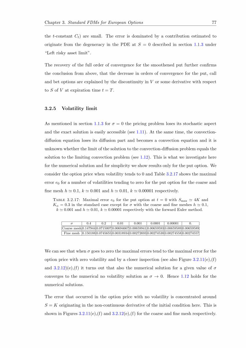
Chapter 3. Standard FDMs for European Options 77
the t-constant Ct) are small. The error is dominated by a contribution estimated to
originate from the degeneracy in the PDE at S = 0 described in section 1.1.3 under
“Left risky asset limit”.
The recovery of the full order of convergence for the smoothened put further confirms
the conclusion from above, that the decrease in orders of convergence for the put, call
and bet options are explained by the discontinuity in V or some derivative with respect
to S of V at expiration time t = T .
3.2.5 Volatility limit
As mentioned in section 1.1.3 for σ = 0 the pricing problem loses its stochastic aspect
and the exact solution is easily accessible (see 1.11). At the same time, the convection-
diffusion equation loses its diffusion part and becomes a convection equation and it is
unknown whether the limit of the solution to the convection-diffusion problem equals the
solution to the limiting convection problem (see 1.12). This is what we investigate here
for the numerical solution and for simplicity we show results only for the put option. We
consider the option price when volatility tends to 0 and Table 3.2.17 shows the maximal
error e0 for a number of volatilities tending to zero for the put option for the coarse and
fine mesh h ' 0.1, k ' 0.001 and h ' 0.01, k ' 0.00001 respectively.
Table 3.2.17: Maximal error e0 for the put option at t = 0 with Smax ' 4K andKα = 0.3 in the standard case except for σ with the coarse and fine meshes h ' 0.1,k ' 0.001 and h ' 0.01, k ' 0.00001 respectively with the forward Euler method.
σ 0.4 0.2 0.01 0.001 0.0001 0.00001 0.
Coarse mesh 0.147944 0.0715007 0.00694667 0.00659941 0.00659593 0.00659589 0.00659589
Fine mesh 0.150188 0.0745655 0.00318934 0.00272693 0.00274538 0.00274558 0.00274557
We can see that when σ goes to zero the maximal errors tend to the maximal error for the
option price with zero volatility and by a closer inspection (see also Figure 3.2.11(e),(f)
and 3.2.12)(e),(f) it turns out that also the numerical solution for a given value of σ
converges to the numerical no volatility solution as σ → 0. Hence 1.12 holds for the
numerical solutions.
The error that occurred in the option price with no volatility is concentrated around
S = K originating in the non-continuous derivative of the initial condition here. This is
shown in Figures 3.2.11(e),(f) and 3.2.12(e),(f) for the coarse and fine mesh respectively.

Chapter 3. Standard FDMs for European Options 78
The leftmost plots of Figures 3.2.11 and 3.2.12 show the changes of option price when
the volatility tends to zero and the rightmost plots show the difference between the
numerical solution with different values of σ and the exact solution with σ = 0 for the
coarse and fine mesh respectively.
Similar results are obtained for the call and bet options leading to the conclusion, that
1.12 holds for the numerical solutions in all cases considered here and probably for a
much wider range of options.

Chapter 3. Standard FDMs for European Options 79
(a) Option Price, σ = 0.2. (b) Error curve, σ = 0.2.
(c) Option Price, σ = 0.001. (d) Error curve, σ = 0.001.
(e) Option Price, σ = 0. (f) Error curve, σ = 0.
Figure 3.2.11: The left curves show option price and the right curves error e0,nNn=1
for the put option at t = 0 with Smax ' 4K and Kα = 0.3 in the standard case exceptfor σ with(a)-(b) σ = 0.2, (c)-(d) σ = 0.001, and (e)-(f) σ = 0 with the coarse mesh
h ' 0.1, k '= 0.001 and with the forward Euler method

Chapter 3. Standard FDMs for European Options 80
(a) Option Price, σ = 0.2. (b) Error curve, σ = 0.2.
(c) Option Price, σ = 0.001. (d) Error curve, σ = 0.001.
(e) Option Price, σ = 0. (f) Error curve, σ = 0.
Figure 3.2.12: The left curves show option price and the right curves error e0,nNn=1
for the put option at t = 0 with Smax ' 4K and Kα = 0.3 in the standard case exceptfor σ with(a)-(b) σ = 0.2, (c)-(d) σ = 0.001, and (e)-(f) σ = 0 with the fine mesh
h ' 0.01, k '= 0.00001 and with the forward Euler method

Chapter 3. Standard FDMs for European Options 81
3.2.6 Expiration limit
We have concluded in subsection 3.2.4 that the singularity at S = K for t = T for the
put, call and bet options give rise to large errors for all values of t down to 0 and for
S-values close to K. Here we investigate the expiration limit i.e. limt↑T V (S, t)−V (S, T )
where V is the numerical solution.
Table 3.2.18: Maximal error e0 for the put option at t = T − k with Smax ' 4K andKα = 0.3 in the standard case with the forward Euler method
@@hk
.1 .01 .001 .0001 .00001 .000001
.5 0.00330986 0.000365137 3.65209e-05 3.65220e-06 3.65200e-07 3.65200e-08
.1 0.00195856 0.000859999 0.000149512 1.49515e-05 1.49515e-06 1.49515e-07.01 0.115326 0.00736102 0.000173821 8.18825e-05 1.40976e-05 1.40977e-06
Table 3.2.19: Maximal error e0 for the put option at t = T −5k with Smax ' 4K andKα = 0.3 in the standard case with the forward Euler method
@@hk
.1 .01 .001 .0001 .00001 .000001
.5 0.00591054 0.00181311 0.000182598 1.82608e-05 1.82600e-06 1.82500e-07
.1 0.000971536 0.00182457 0.000647555 7.47198e-05 7.47536e-06 7.47550e-07.01 921821 4.51905 8.46229e-05 0.00018975 6.13366e-05 7.04452e-06
Table 3.2.20: Maximal error e0 for the call option at t = T − k with Smax ' 4K andKα = 0.3 in the standard case with the forward Euler method
@@hk
.1 .01 .001 .0001 .00001 .000001
.5 0.00331785 0.000365217 3.65217e-05 3.65217e-06 3.65217e-07 3.65217e-08
.1 0.00196655 0.000860079 0.000149513 1.49515e-05 1.49515e-06 1.49515e-07.01 0.115334 0.0073611 0.000173821 8.18826e-05 1.40976e-05 1.40977e-06
Table 3.2.21: Maximal error e0 for the call option at t = T −5k with Smax ' 4K andKα = 0.3 in the standard case with the forward Euler method
@@hk
.1 .01 .001 .0001 .00001 .000001
.5 0.00594985 0.00181351 0.000182602 1.82608e-05 1.82609e-06 1.82609e-07
.1 0.00676164 0.00182497 0.000647559 7.47198e-05 7.47535e-06 7.47569e-07.01 1.16591e+06 4.51905 0.000173821 0.000189751 6.13366e-05 7.04452e-06
Table 3.2.22: Maximal error e0 for the bet option at t = T − k with Smax ' 4K andKα = 0.5 in the standard case with the forward Euler method
@@hk
.1 .01 .001 .0001 .00001 .000001
.5 0.00352959 0.000360024 3.60002e-05 3.60000e-06 3.60000e-07 3.60000e-08
.1 0.00479606 0.00433301 0.00066 6.60000e-05 6.60000e-06 6.60000e-07.01 5.9237 0.486603 0.00422699 0.00415875 0.000606 6.06000e-05

Chapter 3. Standard FDMs for European Options 82
Table 3.2.23: Maximal error e0 for the bet option at t = T −5k with Smax ' 4K andKα = 0.5 in the standard case with the forward Euler method
@@hk
.1 .01 .001 .0001 .00001 .000001
.5 0.00945254 0.00178699 0.00017987 1.79987e-05 1.79999e-06 1.80000e-07
.1 0.00479606 0.014457 0.00317254 0.000329586 3.29959e-05 3.29996e-06.01 1.21441e+08 627.543 0.00422699 0.013079 0.00293048 0.000302635
Table 3.2.24: Maximal error e0 for the smoothened put option at t = T − k withSmax ' 30K in the standard case with the forward Euler method
@@hk
.1 .01 .001 .0001 .00001 .000001
.5 0.00016328 1.55526e-05 1.55440e-06 2.71270e-07 1.18485e-05 4.90119e-05
.1 1.64707e-05 8.41900e-07 1.34900e-07 1.21080e-06 1.57217e-05 8.20377e-05.01 9.28420e-06 1.04300e-07 2.99900e-07 2.52440e-06 2.14538e-05 0.000283342
Table 3.2.25: Maximal error e0 for the smoothened put option at t = T − 5k withSmax ' 30K in the standard case with the forward Euler method
@@hk
.1 .01 .001 .0001 .00001 .000001
.5 0.000814118 7.77619e-05 7.74500e-06 7.80100e-07 1.58410e-06 1.18576e-05
.1 8.17004e-05 4.19010e-06 3.73600e-07 4.12400e-07 3.49770e-06 4.63119e-05.01 1551.52 0.0151725 1.21505e-07 5.16000e-07 3.85330e-06 3.60322e-05

Chapter 3. Standard FDMs for European Options 83
3.3 Numerical results for the backward Euler method
In this section we consider the Backward Euler method for the standard case T = 1,
K = 1, B = 0.3, r = 0.04, γ = 0 and σ = 0.2 with the same computational setup as
described in section 3.2.1. Since the backward Euler method is implicit, the computing
times are significantly higher than for the forward Euler method.
3.3.1 Computational results for the standard case
First we compute the maximal error e0 (see 3.4) at time t = 0 with Smax ' 4K, 2K, 1.5K
and 1.25K for the put option in the standard case with the backward Euler method. The
results are shown in tables 3.3.1–3.3.4. Also the errors e0, nNn=1 (see 3.5) are plotted in
Figures 3.3.1–3.3.2 for a coarse and a fine mesh and Smax ' 4K, 2K, 1.5K and 1.25K.
Table 3.3.1: Maximal error e0 for the put option at t = 0 for Smax ' 4K and Kα = 0.3in the standard case with the backward Euler method.
@@hk
.3 .2 .1 .01 .001 .0001
.5 0.00609529 0.00633076 0.00651671 0.00669163 0.00670955 0.00671134
.4 0.00384639 0.00362807 0.00377233 0.00402266 0.00404835 0.00405093
.3 0.00462138 0.00411196 0.003704 0.00331544 0.00327538 0.00327136
.2 0.00448745 0.00372868 0.00311489 0.00252487 0.00246372 0.00245758
.1 0.00345368 0.00230403 0.00141278 0.000619103 0.000563741 0.000558176.08 0.00328116 0.00210526 0.00120253 0.000406398 0.000349258 0.000343511.06 0.00322514 0.00202104 0.00109011 0.000283795 0.000221138 0.000214835.05 0.00323412 0.00201015 0.0010629 0.000225674 0.000163177 0.000156889.04 0.00323177 0.00199248 0.00103742 0.000174862 0.000108983 0.00010236.03 0.00321785 0.00197012 0.0010115 0.000134884 6.34725e-5 5.69204e-5.02 0.00319782 0.00194879 0.000990868 0.00011523 3.35668e-5 2.70425e-5.01 0.00318483 0.00193659 0.000978546 0.000102356 1.41839e-5 7.41565e-6.001 0.00317989 0.00193236 0.000974538 9.81804e-5 9.86248e-6 1.02276e-6

Chapter 3. Standard FDMs for European Options 84
Table 3.3.2: Maximal error e0 for the put option at t = 0 for Smax ' 2K and Kα = 0.3in the standard case with the backward Euler method
@@hk
.3 .2 .1 .01 .001 .0001
.5 0.00592172 0.00618406 0.00639076 0.00658473 0.00660456 0.00660655
.4 0.00384835 0.00362908 0.00376364 0.0040174 0.00404339 0.004046
.3 0.00462213 0.00411226 0.00370411 0.00331547 0.0032754 0.00327138
.2 0.00448786 0.00372881 0.00311492 0.00252487 0.00246373 0.00245759
.1 0.00345381 0.00230406 0.00141279 0.000619103 0.000563741 0.000558176.08 0.00328127 0.00210527 0.00120253 0.000406398 0.000349258 0.000343511.06 0.0032253 0.00202108 0.00109011 0.000283796 0.000221138 0.000214835.05 0.00323426 0.00201018 0.0010629 0.000225674 0.000163177 0.000156889.04 0.00323189 0.0019925 0.00103742 0.000174862 0.000108983 0.00010236.03 0.00321795 0.00197013 0.0010115 0.000134884 6.34725e-5 5.69205e-5.02 0.00319791 0.00194881 0.000990869 0.00011523 3.35668e-5 2.70425e-5.01 0.00318492 0.0019366 0.000978547 0.000102356 1.41839e-5 8.75748e-6.001 0.00317997 0.00193237 0.000974539 9.81804e-5 9.8625e-6 8.21241e-06
Table 3.3.3: Maximal error e0 for the put option at t = 0 for Smax ' 1.5K andKα = 0.3 in the standard case with the backward Euler method
@@hk
.3 .2 .1 .01 .001 .0001
.5 0.00608397 0.00618406 0.00639076 0.00658473 0.00660456 0.00660655
.4 0.00375692 0.00366857 0.00348810 0.00367456 0.00370539 0.00370848
.3 0.00431481 0.00411786 0.00370732 0.00331706 0.00327687 0.00327283
.2 0.00404811 0.00375119 0.00312869 0.00253232 0.00247063 0.00246444
.1 0.00275091 0.00231131 0.00141581 0.00065754 0.00065754 0.00065754.08 0.00257032 0.00212018 0.00120921 0.00104401 0.00104401 0.00104401.06 0.00251582 0.00204956 0.00109854 0.00105242 0.00105242 0.00105242.05 0.00249824 0.00202773 0.00107062 0.00084084 0.00084084 0.00084084.04 0.00249322 0.00201610 0.00106134 0.00106134 0.00106134 0.00106134.03 0.00246513 0.00198700 0.00101864 0.00093185 0.00093185 0.00093185.02 0.00244382 0.00196552 0.00099786 0.00097696 0.00097696 0.00097696.01 0.00243401 0.00195532 0.00102750 0.00102750 0.00102750 0.00102750.001 0.00243205 0.00195318 0.00107541 0.00107541 0.00107541 0.00107541
Table 3.3.4: Maximal error e0 for the put option at t = 0 for Smax ' 1.25K andKα = 0.3 in the standard case with the backward Euler method
@@hk
.3 .2 .1 .01 .001 .0001
.5 0.00612437 0.00612437 0.00612437 0.00612437 00612437 0.00612437
.4 0.00375692 0.00366857 0.0034881 0.00367456 00370539 0.00370848
.3 0.00446444 0.00425374 0.00381534 0.0033999 0.0033572 0.00335292
.2 0.00532862 0.00532862 0.00532862 0.00532862 0.00532862 0.00532862
.1 0.0087067 0.0087067 0.0087067 0.0087067 0.0087067 0.0087067.08 0.00762432 0.00762432 0.00762432 0.00762432 0.00762432 0.00762432.06 0.0080478 0.0080478 0.0080478 0.0080478 0.0080478 0.0080478.05 0.0074617 0.0074617 0.0074617 0.0074617 0.0074617 0.0074617.04 0.00851633 0.00851633 0.00851633 0.00851633 0.00851633 0.00851633.03 0.00933452 0.00933452 0.00933452 0.00933452 0.00933452 0.00933452.02 0.00942338 0.00942338 0.00942338 0.00942338 0.00942338 0.00942338.01 0.00913899 0.00913899 0.00913899 0.00913899 0.00913899 0.00913899.001 0.0095676 0095676 0.0095676 0.0095676 0.0095676 0.0095676

Chapter 3. Standard FDMs for European Options 85
(a) BE error, coarse mesh, Smax ' 4K. (b) BE error, coarse mesh, Smax ' 2K.
(c) BE error, coarse mesh, Smax ' 1, 5K. (d) BE error, coarse mesh, Smax ' 1.25K.
Figure 3.3.1: Error e0,nNn=1 at t = 0 for the put option and Smax ' (a) 4K, (b)2K, (c) 1.5K and (d) 1.25K for stepsizes h ' 0.1 and k ' 0.01 and Kα = 0.3 in the
standard case with the backward Euler method.

Chapter 3. Standard FDMs for European Options 86
(a) BE error, fine mesh, Smax ' 4K. (b) BE error, fine mesh, Smax ' 2K.
(c) BE error, fine mesh, Smax ' 1, 5K. (d) BE error, fine mesh, Smax ' 1.25K.
Figure 3.3.2: Error e0,nNn=1 at t = 0 for the put option and Smax ' (a) 4K, (b)2K, (c) 1.5K and (d) 1.25K for stepsizes h ' 0.01 and k ' 0.001 and Kα = 0.3 in the
standard case with the backward Euler method.

Chapter 3. Standard FDMs for European Options 87
Next we consider the maximal error e0 at time t = 0 with Smax ' 4K for the call
option in the standard case with the backward Euler method. The results are shown in
Table 3.3.5.
Table 3.3.5: Maximal error e0 for the call option at t = 0 with Smax ' 4K andKα = 0.3 in the standard case with the backward Euler method.
@@hk
.3 .2 .1 .01 .001 .0001
.5 0.00584133 0.00617784 0.00644005 0.00668395 0.00670878 .00671127
.4 0.00410038 0.00378099 0.00369567 0.00401498 0.00404758 0.00405085
.3 0.00487537 0.00426488 0.00378066 0.00332312 0.00327615 0.00327144
.2 0.00474144 0.0038816 0.00319155 0.00253255 0.00246449 0.00245766
.1 0.00370767 0.00245695 0.00148944 0.000611419 0.000562973 0.000558099.08 0.00353515 0.00225818 0.00127919 0.000398713 0.00034849 0.000343434.06 0.00347913 0.00217397 0.00116677 0.000276111 0.00022037 0.000214758.05 0.00348811 0.00216308 0.00113956 0.000218683 0.000162408 0.000156813.04 0.00348576 0.00214541 0.00111408 0.000176433 0.000108215 0.000102283.03 0.00347183 0.00212304 0.00108816 0.000142568 6.27039e-5 5.68435e-5.02 0.00345181 0.00210172 0.00106753 0.000122914 3.27982e-5 2.69657e-5.01 0.00343882 0.00208951 0.00105521 0.00011004 1.49526e-5 7.33879e-6.001 0.00343326 0.00208528 0.0010512 0.000105865 1.06311e-5 1.11788e-6
Now we consider the maximal error e0 at time t = 0 with Smax ' 4K for the bet
option in the standard case with the backward Euler method. The results are shown in
Table 3.3.6. Finally we consider the maximal error e0 at time t = 0 with Smax ' 30K
Table 3.3.6: Maximal error e0 for the bet option at t = 0 with Smax ' 4K andKα = 0.5 in the standard case with the backward Euler method.
@@hk
.3 .2 .1 .01 .001 .0001
.5 0.0191664 0.0184684 0.0179142 0.0173906 0.0173369 0.0173315
.4 0.0191664 0.0184684 0.0179142 0.0173906 0.0173369 0.0173315
.3 0.0233774 0.0220285 0.0209460 0.0199133 0.0198068 0.0197961
.2 0.0193172 0.0163493 0.0139397 0.0116225 0.0113826 0.0113586
.1 0.0102039 0.0075571 0.0053355 0.0031568 0.0029305 0.0029078.08 0.0098829 0.0068268 0.0043824 0.0021216 0.0018953 0.0018726.06 0.0084057 0.0056381 0.0033703 0.0012254 0.0010078 0.0009860.05 0.0084496 0.0054217 0.0030508 0.0009371 0.0007381 0.0007181.04 0.0079794 0.0051162 0.0028181 0.0006869 0.0004774 0.0004580.03 0.0078160 0.0049174 0.0026128 0.0004926 0.0002892 0.0002689.02 0.0077169 0.0047655 0.0024506 0.0003494 0.0001392 0.0001188.01 0.0076450 0.0046647 0.0023648 0.0002628 0.0000525 0.0000317.001 0.0076188 0.0046369 0.0023344 0.0002343 0.0000237 2.63038e-6
for the smoothened put option in the standard case with the backward Euler method.
The results are shown in Table 3.3.7.

Chapter 3. Standard FDMs for European Options 88
Table 3.3.7: Maximal error e0 for the smoothened put option at t = 0 with Smax '30K in the standard case with the backward Euler method.
@@hk
.3 .2 .1 .01 .001 .0001
.5 0.00133865 0.00137846 0.00145861 0.00153132 0.00153862 0.00153935
.4 0.000528457 0.000570851 0.000656069 0.000733258 0.000741002 0.000741777
.3 0.000222407 0.000260449 0.000337129 0.000406829 0.000413835 0.000414536
.2 9.80089e-005 0.000116921 0.000200182 0.000275735 0.000283323 0.000284082
.1 0.000157431 0.000117528 3.74274e-005 6.60896e-005 7.36013e-005 7.43528e-005.08 0.000176201 0.000136901 5.8008e-005 3.63254e-005 4.39059e-005 4.46643e-005.06 0.000192115 0.000149016 6.82257e-005 1.79547e-005 2.56681e-005 2.64405e-005.05 0.000199072 0.000155875 7.15357e-005 1.07863e-005 1.84008e-005 1.9174e-005.04 0.000205495 0.000162334 7.56172e-005 4.36875e-006 1.15366e-005 1.23051e-005.03 0.000211081 0.000167848 8.09551e-005 6.3233e-006 5.88777e-006 6.65884e-006.02 0.000214585 0.000171347 8.44484e-005 7.25001e-006 2.2793e-006 3.04957e-006.01 0.000216855 0.000173615 8.67112e-005 8.01286e-006 7.10504e-007 7.05265e-007.001 0.000217601 0.000174376 8.74691e-005 8.76639e-006 8.70483e-007 4.77757e-007
3.3.2 Computational results for nonstandard cases
Here we consider robustness in the selection of Smax against variations in the other
parameters in the problem when solving with the backward Euler method like we have
done for the forward Euler method in section 3.2.2. As we have mentioned before, since
backward Euler is an implicit method it is also computationally more demanding than
the forward Euler method. Therefore we choose somewhat coarser meshes both for the
coarse mesh and for the fine mesh calculations. We choose a coarse mesh with h ' 0.1
and k ' 0.01 and a fine mesh with h ' 0.01 and k ' 0.001. For each mesh, we shall
find the smallest value of Smax where the error in S = Smax is negligible compared to
the maximal error e0.
As observed when solving with the forward Euler method, we expect no significant
differences between the results for the put, call and bet options. Hence we compute only
for the put option. The results for the coarse mesh are shown in Tables 3.3.8 and 3.3.9
and the results for the fine mesh are shown in Tables 3.3.10 and 3.3.11. In Figure 3.3.3
we show e0,nNn=0 (see 3.5) for the standard case except for T = 0.1 and T = 10 for the
coarse and fine meshes. Figure 3.3.3(a) and (b) should be compared to Figure 3.3.1(a)
and Figure 3.3.3(c) and (d) should be compared to Figure3.3.2(a).

Chapter 3. Standard FDMs for European Options 89
Table 3.3.8: Smallest Smax not giving significant error at S = Smax with the coarsemesh h ' 0.1, k ' 0.01 and Kα = 0.3 in various nonstandard cases for the put optionwith the backward Euler method. “-” indicates a case where it has not been possible
to establish a functional Smax.
K = 10 K = 1 K = 0.1
T = 10
@@rσ
.01 .2 .9
.001 1.25K - -.04 1.25K - -.1 1.25K 6K -
@@rσ
.01 .2 .9
.001 1.5K 15K -.04 3K 10K -.1 4K 4K -
@@rσ
.01 .2 .9
.001 4K 14K -.04 8K 8K -.1 10K 4K -
T = 1
@@rσ
.01 .2 .9
.001 1.25K 3K -.04 1.25K 3K -.1 1.25K 3K -
@@rσ
.01 .2 .9
.001 1.5K 3K 70K.04 2K 3K 60K.1 2K 3K 60K
@@rσ
.01 .2 .9
.001 4K 5K 50K.04 4K 5K 40K.1 4K 4K 30K
T = .1
@@rσ
.01 .2 .9
.001 1.25K 1.5K 4K.04 1.25K 1.5K 4K.1 1.25K 1.5K 4K
@@rσ
.01 .2 .9
.001 1.5K 2K 4K.04 1.5K 2K 4K.1 1.5K 2K 4K
@@rσ
.01 .2 .9
.001 4K 4K 7K.04 4K 4K 7K.1 4K 4K 7K
Table 3.3.9: Smallest Smax not giving significant error at S = Smax with the coarsemesh h ' 0.1, k ' 0.01 and Kα = 0.3 in the standard case except for γ in the put
option with the backward Euler method.
γ 0 0.5 1.0minSmax 3K 3K 5K
Table 3.3.10: Smallest Smax not giving significant error at S = Smax with the finemesh h ' 0.01, k ' 0.001 and Kα = 0.3 in various nonstandard fine for the put optionwith the backward Euler method. “-” indicates a case where it has not been possible
to establish a functional Smax.
K = 10 K = 1 K = 0.1
T = 10
@@rσ
.01 .2 .9
.001 - - -.04 - - -.1 - - -
@@rσ
.01 .2 .9
.001 1.25K - -.04 1.25K - -.1 1.25K - -
@@rσ
.01 .2 .9
.001 1.5K 20K -.04 3K 15K -.1 4K 4K -
T = 1
@@rσ
.01 .2 .9
.001 1.25K - -.04 1.25K - -.1 1.25K - -
@@rσ
.01 .2 .9
.001 1.25K 3K -.04 1.25K 3K -.1 1.25K 3K -
@@rσ
.01 .2 .9
.001 1.5K 3K 50K.04 1.5K 3K 50K.1 2K 3K 50K
T = .1
@@rσ
.01 .2 .9
.001 1.25K 1.5K 4K.04 1.25K 1.5K 4K.1 1.25K 1.5K 4K
@@rσ
.01 .2 .9
.001 1.25K 1.5K 4K.04 1.25K 1.5K 4K.1 1.25K 1.5K 4K
@@rσ
.01 .2 .9
.001 1.5K 2K 4K.04 1.5K 2K 4K.1 1.5K 2K 4K

Chapter 3. Standard FDMs for European Options 90
Table 3.3.11: Smallest Smax not giving significant error at S = Smax with the finemesh h ' 0.01, k ' 0.001 and Kα = 0.3 in the standard case except for γ in the put
option with the backward Euler method.
γ 0 0.5 1.0minSmax 3K 3K 5K
(a) BE error, coarse mesh, T = 0.1. (b) BE error, coarse mesh, T = 10.
(c) BE error, fine mesh, T = 0.1. (d) BE error, fine mesh, T = 10.
Figure 3.3.3: Error e0,nNn=1 at t = 0 for the put option with Smax ' 4K (a) h ' 0.1,k ' 0.01, T = 0.1, (b) h ' 0.1, k ' 0.01, T = 10, (c) h ' 0.01, k ' 0.001, T = 0.1 and(d) h ' 0.01, k ' 0.001, T = 10 and Kα = 0.3, in the standard case apart from the
value of T with the backward Euler method.

Chapter 3. Standard FDMs for European Options 91
3.3.3 Sensitivity to Smax
Tables 3.3.8 and 3.3.10 show the smallest Smax with the backward Euler method are
very similar to tables 3.2.9 and 3.2.11 show the smallest Smax with the forward Euler
method. There is a big difference however. Whereas the forward Euler method is only
conditionally stable, the backward Euler method is unconditionally stable. Hence the
large values of Smax for the backward Euler case — in particular for σ = 0.9 but also in
some cases for σ = 0.2 — can not be explained by instability as we did for the forward
Eular case. We may “discard” the results with σ = 0.9 as being extreme cases since
σ > 0.5 is generally considered such, but this is not sufficient to explain the results.
Instead looking at the error plots corresponding to the ones in Figure 3.3.3 — which are
the ones used for deciding on the minimal Smax — it seems that the error originating
near S = K from the discontinuity in the first derivative in the terminal condition decay
more and more slowly as σ is increasing. Hence the reason for the non-vanishing error
in S = Smax is not that the boundary condition is introducing an error, but that the
error from S = K has simply not yet vanished. For example for the coarse mesh h = 0.1
and k = 0.01 in the case T = 10, K = 0.1, B = 0.3, r = 0.001, γ = 0 and σ = 0.2 the
maximal error with the “preferred” Smax = 14K is e0 = 0.0020457 whereas the maximal
error with Smax = 4K is almost the same, namely e0 = 0.0020464.
Hence the results with the backward Euler method confirm the results with the forward
Euler method: Smax ' 4K seems to be adequate independently of the numerical scheme
used for the solution.
3.3.4 Convergence
First we consider the put option in the standard case with Smax = 4K solved with the
backward Euler method. Plotting the maximal errors e0 (see 3.4) at time t = 0 from
Table 3.3.1 with logarithmic axes, we get the result shown in Figure 3.3.4. From the
data in Table 3.3.1 we get the following convergence result:
e0 ' 0.069h2 + 0.006k (3.12)
Unlike what is observed for the forward Euler method, here we get the expected quadratic
convergence in S and linear convergence in t.
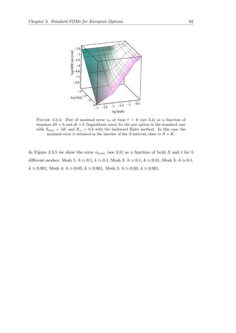
Chapter 3. Standard FDMs for European Options 92
Figure 3.3.4: Plot of maximal error e0 at time t = 0 (see 3.4) as a function ofstepsizes dS = h and dt = k (logarithmic axes) for the put option in the standard casewith Smax = 4K and Kα = 0.3 with the backward Euler method. In this case the
maximal error is attained in the interior of the S-interval, close to S = K.
In Figure 3.3.5 we show the error e0,nm (see 3.8) as a function of both S and t for 5
different meshes: Mesh 1: h ' 0.1, k ' 0.1, Mesh 2: h ' 0.1, k ' 0.01, Mesh 3: h ' 0.1,
k ' 0.001, Mesh 4: h ' 0.05, k ' 0.001, Mesh 5: h ' 0.03, k ' 0.001.

Chapter 3. Standard FDMs for European Options 93
(a) Mesh 1 error. (b) Mesh 2 error.
(c) Mesh 3 error.
(d) Mesh 4 error. (e) Mesh 5 error.
Figure 3.3.5: Plot of the error as a function of S and t for the put option withSmax = 4K and Kα = 0.3 with the backward Euler method for mesh 1 (a), mesh 2 (b),
mesh 3 (c), mesh 4 (d) and mesh 5 (e).

Chapter 3. Standard FDMs for European Options 94
Figure 3.3.6: Plot of maximal error e0 at time t = 0 (see 3.4) as a function ofstepsizes dS = h and dt = k (logarithmic axes) for the call option in the standard casewith Smax = 4K and Kα = 0.3 with the backward Euler method. In this case the
maximal error is attained in the interior of the S-interval, close to S = K.
Next we turn to the call option in the standard case with Smax = 4K solved with the
backward Euler method. Plotting the maximal errors e0 (see 3.4) at time t = 0 from
Table 3.3.5 with logarithmic axes, we get the result shown in Figure 3.3.6. From the
data in Table 3.3.5 we get the following convergence result:
e0 ' 0.07h2 + 0.006k (3.13)
Unlike what is observed for the forward Euler method, here we get the expected quadratic
convergence in S and linear convergence in t.
Then we consider the bet option in the standard case with Smax = 4K solved with the
backward Euler method. Plotting the maximal errors e0 (see 3.4) at time t = 0 from
Table 3.3.6 with logarithmic axes, we get the result shown in Figure 3.3.7. From the
data in Table 3.3.6 we get the following convergence result:
e0 ' 0.016h1.4 + 0.001k (3.14)
As observed for the forward Euler method, for the bet option we get a reduction in the
expected quadratic convergence in S. We still observe the expected linear convergence
in t.

Chapter 3. Standard FDMs for European Options 95
Figure 3.3.7: Plot of maximal error e0 at time t = 0 (see 3.4) as a function ofstepsizes dS = h and dt = k (logarithmic axes) for the bet option in the standard casewith Smax = 4K and Kα = 0.5 with the backward Euler method. In this case the
maximal error is attained in the interior of the S-interval, close to S = K.
Finally we consider the smoothened put option in the standard case with Smax = 30K
solved with the backward Euler method. Plotting the maximal errors e0 (see (3.4)) at
time t = 0 from Table 3.3.7 with logarithmic axes, we get the result shown in Figure 3.3.8
with the following convergence result:
e0 ' 0.005h2 + 0.01k (3.15)
For comparison, the convergence results with the backward Euler method are repeated
here:
Put: e0 ' 0.069h2 + 0.006k
Call: e0 ' 0.07h2 + 0.006k
Bet: e0 ' 0.016h1.4 + 0.001k
Smoothened put: e0 ' 0.005h2 + 0.01k
The conclusion is that the discontinuity in the derivative ∂V∂S at (S, t) = (K,T ) for the
put and call options shows up in the computational results, but that we observe no loss
of convergence neither in t nor in S (with respect to the expected linear convergence in
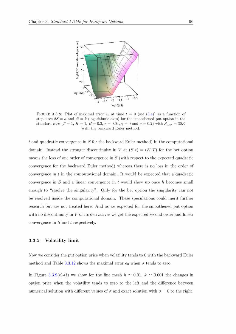
Chapter 3. Standard FDMs for European Options 96
Figure 3.3.8: Plot of maximal error e0 at time t = 0 (see (3.4)) as a function ofstep sizes dS = h and dt = k (logarithmic axes) for the smoothened put option in thestandard case (T = 1, K = 1, B = 0.3, r = 0.04, γ = 0 and σ = 0.2) with Smax = 30K
with the backward Euler method.
t and quadratic convergence in S for the backward Euler method) in the computational
domain. Instead the stronger discontinuity in V at (S, t) = (K,T ) for the bet option
means the loss of one order of convergence in S (with respect to the expected quadratic
convergence for the backward Euler method) whereas there is no loss in the order of
convergence in t in the computational domain. It would be expected that a quadratic
convergence in S and a linear convergence in t would show up once h becomes small
enough to “resolve the singularity”. Only for the bet option the singularity can not
be resolved inside the computational domain. These speculations could merit further
research but are not treated here. And as we expected for the smoothened put option
with no discontinuity in V or its derivatives we get the expected second order and linear
convergence in S and t respectively.
3.3.5 Volatility limit
Now we consider the put option price when volatility tends to 0 with the backward Euler
method and Table 3.3.12 shows the maximal error e0 when σ tends to zero.
In Figure 3.3.9(e)-(f) we show for the fine mesh h ' 0.01, k ' 0.001 the changes in
option price when the volatility tends to zero to the left and the difference between
numerical solution with different values of σ and exact solution with σ = 0 to the right.

Chapter 3. Standard FDMs for European Options 97
Table 3.3.12: Maximal error e0 for the put option at t = 0 with Smax ' 4KandKα = 0.3 in the standard case except σ with the coarse and fine meshes h ' 0.1,k ' 0.01 and h ' 0.01, k ' 0.001 respectively with the backward Euler method.
σ 0.4 0.2 0.01 0.001 0.0001 0.00001 0.
Coarse mesh 0.147722 0.0714003 0.00698829 0.00664124 0.00663775 0.00663772 0.00663772
Fine mesh 0.150168 0.0745572 0.00320859 0.00270294 0.00272136 0.00272155 0.00272155
We conclude, as for the forward Euler method, that the numerical solutions computed
with the backward Euler method satisfy 1.12.

Chapter 3. Standard FDMs for European Options 98
(a) Option Price, σ = 0.2. (b) Error curve, σ = 0.2.
(c) Option Price, σ = 0.001. (d) Error curve, σ = 0.001.
(e) Option Price, σ = 0. (f) Error curve, σ = 0.
Figure 3.3.9: The left curves show option price and the right curves error e0,nNn=1
for the put option at t = 0 with Smax ' 4K and Kα = 0.3 in the standard case exceptfor σ with(a)-(b) σ = 0.2, (c)-(d) σ = 0.001, and (e)-(f) σ = 0 with the fine mesh
h ' 0.01, k '= 0.001 and with the backward Euler method

Chapter 3. Standard FDMs for European Options 99
3.3.6 Expiration limit
Here we compute the expiration limit for the options as we did in subsection 3.2.6 with
the for ward Euler method.
Table 3.3.13: Maximal error e0 for the put option at t = T − k with Smax ' 4K andKα = 0.3 in the standard case with the backward Euler method
@@hk
.1 .01 .001 .0001 .00001 .000001
.5 0.00331879 0.000365234 3.65219e-05 3.65218e-06 3.65217e-07 3.65217e-08
.1 0.00184363 0.000824394 0.00014914 1.49477e-05 1.49511e-06 1.49514e-07.01 0.0028557 0.000898223 0.00019204 7.77653e-05 1.40544e-05 1.40934e-06
Table 3.3.14: Maximal error e0 for the put option at t = T −5k with Smax ' 4K andKα = 0.3 in the standard case with the backward Euler method
@@hk
.1 .01 .001 .0001 .00001 .000001
.5 0.00565441 0.00181357 0.000182603 1.82608e-05 1.82609e-06 1.82609e-07
.1 0.0020224 0.00178869 0.000645733 7.47011e-05 7.47517e-06 7.47567e-07.01 0.00139073 000454277 0.000201432 0.000189783 6.11255e-05 7.04235e-06
Table 3.3.15: Maximal error e0 for the call option at t = T − k with Smax ' 4K andKα = 0.3 in the standard case with the backward Euler method
@@hk
.1 .01 .001 .0001 .00001 .000001
.5 0.00331084 0.000365154 3.65211e-05 3.65217e-06 3.65217e-07 3.65217e-08
.1 0.00185158 0.000824314 0.000149139 1.49477e-05 1.49511e-06 1.49514e-07.01 0.00286365 0.000898302 0.00019204 7.77653e-05 1.40544e-05 1.40934e-06
Table 3.3.16: Maximal error e0 for the call option at t = T −5k with Smax ' 4K andKα = 0.3 in the standard case with the backward Euler method
@@hk
.1 .01 .001 .0001 .00001 .000001
.5 0.00561531 0.00181317 0.000182599 1.82608e-05 1.82609e-06 1.82609e-07
.1 0.00206151 0.00178829 0.000645729 7.47011e-05 7.47517e-06 7.47567e-07.01 0.00142983 000454676 0.000201436 0.000189783 6.11255e-05 7.04235e-06
Table 3.3.17: Maximal error e0 for the bet option at t = T − k with Smax ' 4K andKα = 0.5 in the standard case with the backward Euler method
@@hk
.1 .01 .001 .0001 .00001 .000001
.5 0.00340489 0.000358709 3.59870e-05 3.59987e-06 3.59999e-07 3.60000e-08
.1 0.02724 0.00394572 0.000655884 6.59586e-05 6.59959e-06 6.59996e-07.01 0.0192518 0.0205107 0262852 0.00381672 000602376 6.05635e-05

Chapter 3. Standard FDMs for European Options 100
Table 3.3.18: Maximal error e0 for the bet option at t = T −5k with Smax ' 4K andKα = 0.5 in the standard case with the backward Euler method
@@hk
.1 .01 .001 .0001 .00001 .000001
.5 0.0102349 0.00178064 0.000179806 1.79981e-05 1.79998e-06 1.80000e-07
.1 0.00944335 0.0160589 0.00315253 0.000329379 3.29938e-05 3.29994e-06.01 0.0045153 0.00467452 0.00957738 0.0144031 0.00291284 0.000302454
3.4 Numerical results for the Crank Nicolson method
In this section we consider the Crank Nicolson method for the standard case T = 1,
K = 1, B = 0.3, r = 0.04, γ = 0 and σ = 0.2 with the same computational setup as
described in sections 3.2.1 and 3.3.1. Since the Crank Nicolson method is an implicit
scheme like the backward Euler method, the computing times are similarly high.
3.4.1 Computational results for the standard case
First we compute the maximal error e0 (see 3.4) at time t = 0 with Smax ' 4K, 2K, 1.5K
and 1.25K for the put option in the standard case with the Crank Nicolson method.
The results are shown in Tables 3.4.1–3.4.4 and in Figures 3.4.1–3.4.2.
Table 3.4.1: Maximal error e0 for the put option at t = 0 for Smax ' 4K and Kα = 0.3in the standard case with the Crank Nicolson method.
@@hk
.3 .2 .1 .01 .001 .0001
.5 0.00672936 0.00671793 0.00671314 0.00671156 0.00671154 0.00671154
.4 0.00408546 0.00406345 0.00405426 0.00405125 0.00405122 0.00405122
.3 0.00322124 0.00325308 0.00326646 0.00327087 0.00327091 0.00327091
.2 0.00233565 0.00241369 0.00244614 0.00245679 0.0024569 0.0024569
.1 0.000501005 0.000536946 0.00055238 0.000557505 0.000557557 0.000557557.08 0.000284197 0.000320717 0.000337337 0.000342817 0.000342872 0.000342872.06 0.000651676 0.000174949 0.000204624 0.00021404 0.000214133 0.000214134.05 0.00113038 0.000126523 0.00014705 0.0001561 0.00015619 0.00015619.04 0.0018367 0.00024821 9.14746e-5 0.000101488 0.000101623 0.000101624.03 0.00290236 0.000737749 4.7315e-5 5.60747e-5 5.61908e-5 5.6192e-5.02 0.00400788 0.00150029 0.000119567 2.62052e-5 2.6316e-5 2.63171e-5.01 0.00534424 0.00265056 0.000704856 6.56793e-6 6.68405e-6 6.68515e-6.001 0.00666172 0.00391332 0.00181799 7.31236e-5 6.65842e-8 6.77993e-8

Chapter 3. Standard FDMs for European Options 101
Table 3.4.2: Maximal error e0 for the put option at t = 0 for Smax ' 2K and Kα = 0.3in the standard case with the Crank Nicolson method.
@@hk
.3 .2 .1 .01 .001 .0001
.5 0.00662353 0.00661279 0.00660828 0.00660679 0.00660677 0.00660677
.4 0.0040794 0.0040581 0.00404923 0.00404632 0.00404629 0.00404629
.3 0.00322131 0.00325312 0.00326649 0.00327089 0.00327094 0.00327094
.2 0.00233568 0.0024137 0.00244615 0.0024568 0.00245691 0.00245691
.1 0.000501005 0.000536946 0.00055238 0.000557505 0.000557557 0.000557557.08 0.000284198 0.000320718 0.000337338 0.000342817 0.000342872 0.000342872.06 0.000651674 0.00017495 0.000204624 0.00021404 0.000214133 0.000214134.05 0.00113038 0.000126523 0.00014705 0.0001561 0.000156189 0.00015619.04 0.00187367 0.00024821 9.14746e-5 0.000101488 0.000101623 0.000101624.03 0.00290235 0.000737749 4.73149e-5 5.60746e-5 5.61908e-5 5.6192e-5.02 0.00400788 0.00150029 0.000119568 2.62052e-5 2.6316e-5 2.63171e-5.01 0.00534424 0.00265056 0.000704857 8.75748e-6 8.75748e-6 8.75748e-6.001 0.00666172 0.00391332 0.00181799 7.31236e-5 8.29540e-6 8.21241e-6
Table 3.4.3: Maximal error e0 for the put option at t = 0 for Smax ' 1.5K andKα = 0.3 in the standard case with the Crank Nicolson method.
@@hk
.3 .2 .1 .01 .001 .0001
.5 0.00661619 0.00661279 0.00660828 0.00660679 0.00660677 0.00660677
.4 0.00372853 0.00372142 0.00371196 0.00370885 0.00370882 0.00370882
.3 0.0032449 0.00325481 0.0032680 0.00327234 0.00327239 0.00327239
.2 0.00239739 0.00242142 00245322 0.00246365 0.00246375 0.00246375
.1 0.000657543 0.000657543 0.000657543 0.000657543 0.000657543 0.00065754.08 0.00104401 0.00104401 0.00104401 0.00104401 0.00104401 0.00104401.06 0.00105242 0.00105242 0.00105242 0.00105242 0.00105242 0.00105242.05 0.000840836 0.000840836 0.000840836 0.000840836 0.00084084 0.00084084.04 0.00106134 0.00106134 0.00106134 0.00106134 0.00106134 0.00106134.03 0.00124797 0.000931848 0.000931848 0.000931848 0.00093185 0.00093185.02 0.00214265 0.0014987 0.000976963 0.000976963 0.00097696 0.00097696.01 0.0033607 0.00264872 0.00102750 0.0010275 0.00102750 0.0010275.001 0.004640 0.00391119 00181926 0.00107541 0.00107541 0.00107541
Table 3.4.4: Maximal error e0 for the put option at t = 0 for Smax ' 1.25K andKα = 0.3 in the standard case with the Crank Nicolson method.
@@hk
.3 .2 .1 .01 .001 .0001
.5 0.00612437 0.00612437 0.00612437 0.00612437 0.00612437 0.00612437
.4 0.00372853 0.00372142 0.00371196 0.00370885 0.00370882 0.00370882
.3 0.00332707 0.00333621 0.00334839 0.00335240 0.00335244 0.00335244
.2 0.00532862 0.00532862 0.00532862 0.00532862 0.00532862 0.00532862
.1 0.0087067 0.0087067 0.00870670 0.00870670 0.00870670 0.00870670.08 0.00762432 0.00762432 0.00762432 0.00762432 0.00762432 0.00762432.06 0.0080478 0.00804780 0.00804780 0.00804780 0.00804780 0.00804780.05 0.0074617 0.00746170 0.00746170 0.0074617 0.00746170 0.00746170.04 0.00851633 0.00851633 0.00851633 0.00851633 0.00851633 0.00851633.03 0.00933452 0.00933452 0.00933452 0.00933452 0.00933452 0.00933452.02 0.00942338 0.00942338 0.00942338 0.00942338 0.00942338 0.00942338.01 0.00913899 0.00913899 0.00913899 0.00913899 0.00913899 0.00913899.001 0.00956760 0.00956760 0.00956760 0.00956760 0.00956760 0.0095676

Chapter 3. Standard FDMs for European Options 102
(a) CN error, coarse mesh, Smax ' 4K. (b) CN error, coarse mesh, Smax ' 2K.
(c) CN error, coarse mesh, Smax ' 1, 5K. (d) CN error, coarse mesh, Smax ' 1.25K.
Figure 3.4.1: Error e0,nNn=1 at t = 0 for the put option and Smax ' (a) 4K, (b)2K, (c) 1.5K and (d) 1.25K for stepsizes h ' 0.1 and k ' 0.01 and Kα = 0.3 in the
standard case with the Cranck Nicolson method.

Chapter 3. Standard FDMs for European Options 103
(a) CN error, fine mesh, Smax ' 4K. (b) CN error, fine mesh, Smax ' 2K.
(c) CN error, fine mesh, Smax ' 1, 5K. (d) CN error, fine mesh, Smax ' 1.25K.
Figure 3.4.2: Error e0,nNn=1 at t = 0 for the put option and Smax ' (a) 4K, (b)2K, (c) 1.5K and (d) 1.25K for stepsizes h ' 0.01 and k ' 0.001 and Kα = 0.3 in the
standard case with the Cranck Nicolson method.

Chapter 3. Standard FDMs for European Options 104
Now we consider the maximal error e0 at time t = 0 with Smax ' 4K for the call
option in the standard case with the Crank Nicolson method. The results are shown in
Table 3.4.5.
Table 3.4.5: Maximal error e0 for the call option at t = 0 for Smax ' 4K and Kα = 0.3in the standard case with the Crank Nicolson method.
@@hk
.3 .2 .1 .01 .001 .0001
.5 0.00672993 0.00671814 0.00671319 0.00671156 0.00671154 0.00671154
.4 0.00408603 0.00406365 0.00405431 0.00405125 0.00405122 0.00405122
.3 0.00322067 0.00325287 0.00326641 0.00327087 0.00327091 0.00327091
.2 0.00233508 0.00241348 0.00244609 0.00245679 0.0024569 0.0024569
.1 0.000501575 0.000537151 0.000552431 0.000557506 0.000557557 0.000557557.08 0.000284767 0.000320923 0.000337389 0.000342817 0.000342872 0.000342872.06 0.000652245 0.000175154 0.000204675 0.00021404 0.000214133 0.000214134.05 0.00113095 0.000126728 0.000147102 0.0001561 0.00015619 0.00015619.04 0.00187424 0.000248416 9.1526e-5 0.000101489 0.000101623 0.000101624.03 0.00290292 0.000737954 4.73664e-5 5.60753e-5 5.61909e-5 5.6192e-5.02 0.00400845 0.0015005 0.000119516 2.62058e-5 2.63161e-5 2.63172e-5.01 0.0053448 0.00265076 0.000704805 6.56847e-6 6.68407e-6 6.68515e-6.001 0.0066619 0.00391352 0.00181794 7.3123e-5 6.65894e-8 6.77994e-8
Finally we consider the maximal error e0 at time t = 0 with Smax ' 4K for the bet
option in the standard case with the Crank Nicolson method. The results are shown in
Table 3.4.6.
Table 3.4.6: Maximal error e0 for the bet option at t = 0 with Smax ' 4K andKα = 0.5 in the standard case with the Crank Nicolson method.
@@hk
.3 .2 .1 .01 .001 .0001
.5 0.0172728 0.0173101 0.0173257 0.0173308 0.0173309 0.0173309
.4 0.0172728 0.0173101 0.0173257 0.0173308 0.0173309 0.0173309
.3 0.0196424 0.0197403 0.0197813 0.0197948 0.0197949 0.0197949
.2 0.0105562 0.0110726 0.0112855 0.0113552 0.0113559 0.0113559
.1 0.0020692 0.0026026 0.0028317 0.0029045 0.0029052 0.00290525.08 0.0020888 0.0016613 0.0017822 0.0018692 0.0018701 0.00187013.06 0.0125431 0.0007964 0.0009074 0.0009828 0.0009836 0.000983583.05 0.0211934 0.0019972 0.0006579 0.0007153 0.0007159 0.000715862.04 0.0356145 0.0073694 0.0004022 0.0004553 0.0004559 0.000455861.03 0.0554435 0.0202956 0.0004334 0.0002660 0.0002666 0.00026659.02 0.0832861 0.0481960 0.0071909 0.0001160 0.0001166 0.000116588.01 0.1156278 0.0931800 0.0479155 0.0000288 0.0000294 0.0000294.001 0.1474289 0.1446246 0.1383441 0.0476325 2.90458e-7 4.83086e-7
3.4.2 Computational results for nonstandard cases
Here we consider robustness in the selection of Smax against variations in the other
parameters in the problem when solving with the Crank Nicolson method like we have

Chapter 3. Standard FDMs for European Options 105
done for the forward and backward Euler methods in sections 3.2.2 and 3.3.2. since
Crank Nicolson method is an implicit method, we choose the same mesh sizes that we
chose for the backward Euler method in section 3.3.2 therefore the coarse mesh with
h ' 0.1 and k ' 0.01 and the fine mesh with h ' 0.01 and k ' 0.001. For each mesh, we
shall find the smallest value of Smax where the error in S = Smax is negligible compared
to the maximal error e0.
As observed when solving with the forward Euler method, we expect no significant
differences between the results for the put, call and bet options. Hence here we compute
only for the put option as well. The results for the coarse mesh are shown in Tables 3.4.7
and 3.4.8 and the results for the fine mesh are shown in Tables 3.4.9 and 3.4.10.
Table 3.4.7: Smallest Smax not giving significant error at S = Smax with the coarsemesh h ' 0.1, k ' 0.01 and Kα = 0.3 in various nonstandard cases for the put optionwith the Crank Nicolson method. “-” indicates a case where it has not been possible
to establish a functional Smax.
K = 10 K = 1 K = 0.1
T = 10
@@rσ
.01 .2 .9
.001 1.25K - -.04 1.25K - -.1 1.25K 5K -
@@rσ
.01 .2 .9
.001 1.25K 8K -.04 1.5K 5K -.1 1.5K 2K -
@@rσ
.01 .2 .9
.001 2K 3K -.04 2K 2K -.1 2K 2K -
T = 1
@@rσ
.01 .2 .9
.001 1.25K 3K -.04 1.25K 3K -.1 1.25K 2K -
@@rσ
.01 .2 .9
.001 1.5K 2K 24K.04 1.5K 2K 23K.1 1.5K 2K 22K
@@rσ
.01 .2 .9
.001 2K 2K 7K.04 2K 2K 6K.1 2K 2K 6K
T = .1
@@rσ
.01 .2 .9
.001 1.25K 1.25K 2K.04 1.25K 1.25K 2K.1 1.25K 1.25K 2K
@@rσ
.01 .2 .9
.001 1.25K 1.25K 3K.04 1.25K 1.25K 3K.1 1.25K 1.25K 3K
@@rσ
.01 .2 .9
.001 2K 2K 2K.04 2K 2K 2K.1 2K 2K 2K
Table 3.4.8: Smallest Smax not giving significant error at S = Smax with the coarsemesh h ' 0.1, k ' 0.01 and Kα = 0.3 in the standard case except for γ in the put
option with the Crank Nicolson method.
γ 0 0.5 1.0minSmax 2K 3K 4K
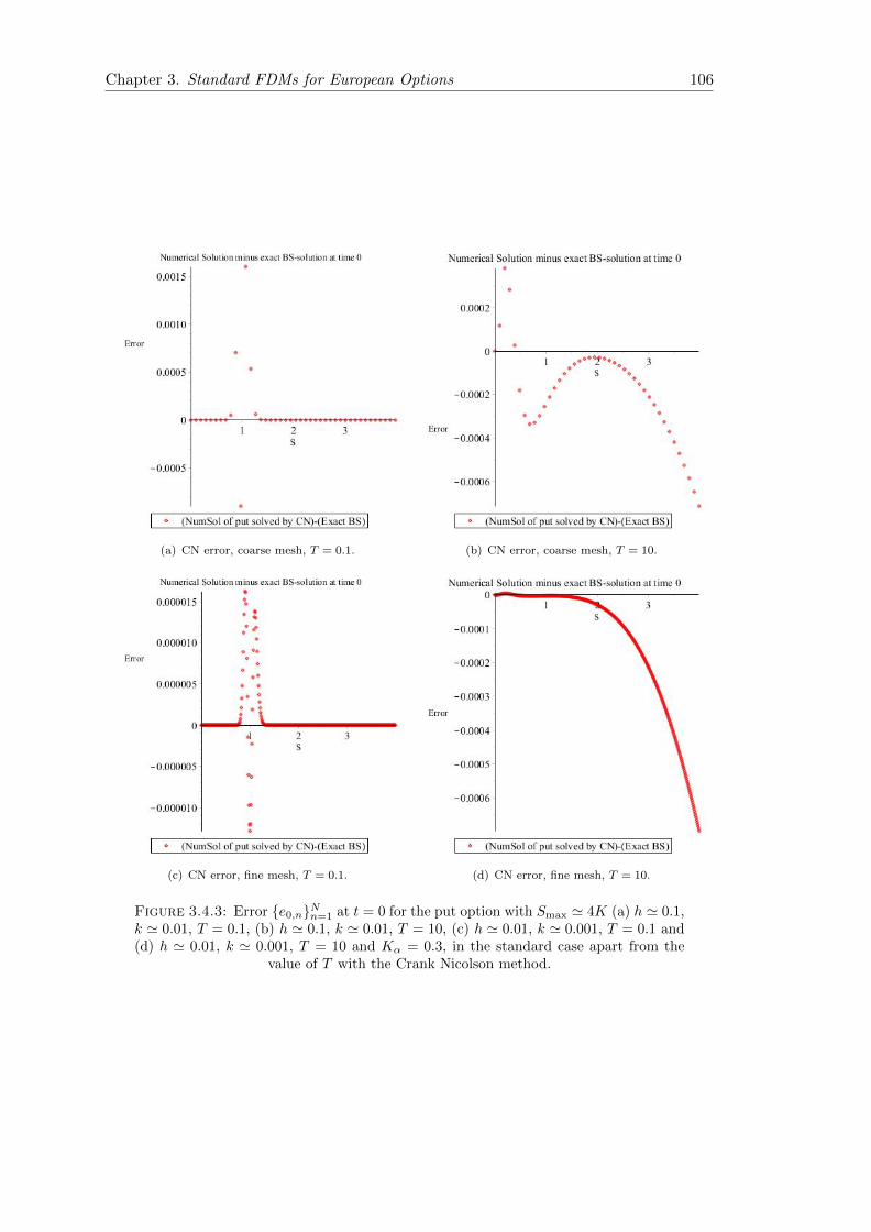
Chapter 3. Standard FDMs for European Options 106
(a) CN error, coarse mesh, T = 0.1. (b) CN error, coarse mesh, T = 10.
(c) CN error, fine mesh, T = 0.1. (d) CN error, fine mesh, T = 10.
Figure 3.4.3: Error e0,nNn=1 at t = 0 for the put option with Smax ' 4K (a) h ' 0.1,k ' 0.01, T = 0.1, (b) h ' 0.1, k ' 0.01, T = 10, (c) h ' 0.01, k ' 0.001, T = 0.1 and(d) h ' 0.01, k ' 0.001, T = 10 and Kα = 0.3, in the standard case apart from the
value of T with the Crank Nicolson method.

Chapter 3. Standard FDMs for European Options 107
Table 3.4.9: Smallest Smax not giving significant error at S = Smax with the finemesh h ' 0.01, k ' 0.001 and Kα = 0.3 in various nonstandard cases for the putoption with the Crank Nicolson method. “-” indicates a case where it has not been
possible to establish a functional Smax.
K = 10 K = 1 K = 0.1
T = 10
@@rσ
.01 .2 .9
.001 - - -.04 - - -.1 - - -
@@rσ
.01 .2 .9
.001 1.25K - -.04 1.25K - -.1 1.25K - -
@@rσ
.01 .2 .9
.001 1.25K 8K -.04 1.25K 5K -.1 1.25K 2K -
T = 1
@@rσ
.01 .2 .9
.001 1.25K - -.04 1.25K - -.1 1.25K - -
@@rσ
.01 .2 .9
.001 1.25K 3K -.04 1.25K 3K -.1 1.25K 2K -
@@rσ
.01 .2 .9
.001 1.25K 2K 25K.04 1.25K 2K 25K.1 1.25K 1.5K 25K
T = .1
@@rσ
.01 .2 .9
.001 1.25K 1.5K 3K.04 1.25K 1.5K 3K.1 1.25K 1.5K 3K
@@rσ
.01 .2 .9
.001 1.25K 1.25K 4K.04 1.25K 1.25K 4K.1 1.25K 1.25K 4K
@@rσ
.01 .2 .9
.001 1.25K 1.25K 3K.04 1.25K 1.25K 3K.1 1.25K 1.25K 3K
Table 3.4.10: Smallest Smax not giving significant error at S = Smax with the coarsemesh h ' 0.01, k ' 0.001 and Kα = 0.3 in the standard case except for γ in the put
option with the Crank Nicolson method.
γ 0 0.5 1.0minSmax 3K 4K 5K
3.4.3 Sensitivity to Smax
Sensitivity to for the Crank-Nicolson method Smax shows there is no indication in the
computations that have been performed that the results would differ from the forward
or backward Euler methods. Thus Smax = 4K still seems to be a fairly good all round
selection for most reasonable parameter values.
3.4.4 Convergence
First we consider the put option in the standard case with Smax = 4K solved with the
Crank Nicolson method. Plotting the maximal errors e0 (see 3.4) at time t = 0 from
Table 3.4.1 with logarithmic axes, we get the result shown in Figure 3.4.4. Obviously
there are 2 significantly different parts of the domain, that we shall refer to as “inside
the bubble”(h ∈]0, 0.08] and k ∈ [0.3, 0.001]) and “outside the bubble”(h ∈ [0.08, 0.5]
and k ∈ [0.001, 0.0001]) respectively. Technically the “bubble” is where the error is
increasing with decreasing dS = h. From the data in Table 3.4.1 we get the following

Chapter 3. Standard FDMs for European Options 108
Figure 3.4.4: Plot of maximal error e0 at time t = 0 (see 3.4) as a function ofstepsizes dS = h and dt = k (logarithmic axes) for the put option in the standard casewith Smax = 4K and Kα = 0.3 with the Crank Nicolson method. In this case the
maximal error is attained in the interior of the S-interval, close to S = K.
convergence result:
e0 '
0.019k1.5 ”in the bubble”
0.069h2 ”outside the bubble”(3.16)
Unlike what is observed for the forward Euler method, here we get the expected quadratic
convergence in S and t, but only in the bubble.
In Figure 3.4.5 we show the error e0,nm (see 3.8) as a function of both S and t for 5
different meshes: Mesh 1: h ' 0.1, k ' 0.1, Mesh 2: h ' 0.1, k ' 0.01, Mesh 3: h ' 0.1,
k ' 0.001, Mesh 4: h ' 0.05, k ' 0.001, Mesh 5: h ' 0.03, k ' 0.001.

Chapter 3. Standard FDMs for European Options 109
(a) Mesh 1 error. (b) Mesh 2 error.
(c) Mesh 3 error.
(d) Mesh 4 error. (e) Mesh 5 error.
Figure 3.4.5: Plot of the error as a function of S and t for the put option withSmax = 4K and Kα = 0.3 with Cranck Nicolson method for mesh 1 (a), mesh 2 (b),
mesh 3 (c), mesh 4 (d) and mesh 5 (e).

Chapter 3. Standard FDMs for European Options 110
Figure 3.4.6: Plot of maximal error e0 at time t = 0 (see 3.4) as a function ofstepsizes dS = h and dt = k (logarithmic axes) for the call option in the standard casewith Smax = 4K and Kα = 0.3 with the Crank Nicolson method. In this case the
maximal error is attained in the interior of the S-interval, close to S = K.
Next we turn to the call option in the standard case with Smax = 4K solved with the
Crank Nicolson method. Plotting the maximal errors e0 (see 3.4) at time t = 0 from
Table 3.4.5 with logarithmic axes, we get the result shown in Figure 3.4.6. Obviously
there are 2 significantly different parts of the domain, that we shall refer to as “inside
the bubble” and “outside the bubble” respectively. From the data in Table 3.4.5 we get
the following convergence result:
e0 '
0.02k1.5 ”in the bubble”
0.07h2 ”outside the bubble”(3.17)
Unlike what is observed for the forward Euler method, here we get the expected quadratic
convergence in S and t, but only in the bubble.
Finally we consider the bet option in the standard case with Smax = 4K solved with the
Crank Nicolson method. Plotting the maximal errors e0 (see 3.4) at time t = 0 from
Table 3.4.6 with logarithmic axes, we get the result shown in Figure 3.4.7. Obviously
there are 2 significantly different parts of the domain, that we shall refer to as “inside
the bubble” and “outside the bubble” respectively. From the data in Table 3.4.6 we get

Chapter 3. Standard FDMs for European Options 111
Figure 3.4.7: Plot of maximal error e0 at time t = 0 (see 3.4) as a function ofstepsizes dS = h and dt = k (logarithmic axes) for the bet option in the standard casewith Smax = 4K and Kα = 0.5 with the Crank Nicolson method. In this case the
maximal error is attained in the interior of the S-interval, close to S = K.
the following convergence result:
e0 '
0.118k0.6 ”in the bubble”
0.017h1.4 ”outside the bubble”(3.18)
Here we are far from getting the expected quadratic convergence in S and t.
For comparison, the convergence results with the Crank Nicolson method are repeated
here:
Put: e0 '
0.019k1.5 ”in the bubble”
0.069h2 ”outside the bubble”
Call: e0 '
0.02k1.5 ”in the bubble”
0.07h2 ”outside the bubble”
Bet: e0 '
0.118k0.6 ”in the bubble”
0.017h1.4 ”outside the bubble”
The conclusion is that the discontinuity in the derivative ∂V∂S at (S, t) = (K,T ) for the
put and call options means the loss of two orders of convergence in t (with respect
to the expected quadratic convergence for the Crank Nicolson method) for bigger step
sizes h in the computational domain. For smaller step sizes h in the computational

Chapter 3. Standard FDMs for European Options 112
domain we observe the full quadratic convergence. Instead the expected quadratic order
of convergence in S is observed in the computational domain. The discontinuity in V
at (S, t) = (K,T ) for the bet option still means the loss of two orders of convergence in
t (with respect to the expected quadratic convergence for the Crank Nicolson method)
for bigger step sizes h in the computational domain. For smaller step sizes h in the
computational domain we still lose more than one order in t because of the stronger
singularity for the bet option than for the put and call options. The stronger singularity
for the bet option (with respect to the put and call options) also means the loss of one
order of convergence in S (with respect to the expected quadratic convergence for the
Crank Nicolson method) in the entire computational domain. It would be expected that
a quadratic convergence in S and t for the bet option would show up once h becomes
small enough to “resolve the singularity”. But because of the strong singularity this
requires such small values of h that they are out of our computational domain. These
speculations could merit further research but are not treated here.
3.4.5 Volatility limit
Now we consider the put option price computed with the Crank-Nicolson method when
volatility tend to 0 and Table 3.4.11 shows the maximal error e0 when σ tends to zero.
Table 3.4.11: Maximal error e0 for the put option with the Crank-Nicolson methodat time 0 with the standard case except σ at Smax ' 4K and Kα = 0.3 with the coarse
and fine meshes h ' 0.1, k ' 0.01 and h ' 0.01, k ' 0.001 respectively.
σ 0.4 0.2 0.01 0.001 0.0001 0.00001 0.
Coarse mesh 0.147924 0.0714919 0.00695045 0.00660321 0.00659973 0.00659969 0.00659969
Fine mesh 0.150188 0.0745654 0.00318953 0.00212712 0.00211662 0.00211651 0.00211651
In Figure 3.4.8 we show for the fine mesh h ' 0.01, k ' 0.001 the changes in option price
when the volatility tends to zero to the left and the difference between the numerical
solution with different values of σ and the exact solution with σ = 0 to the right.
We conclude, as for the forward and backward Euler methods, that the numerical solu-
tions computed with the Crank-Nicolson method satisfy 1.12.

Chapter 3. Standard FDMs for European Options 113
(a) Option Price, σ = 0.2, fine mesh. (b) Error curve, σ = 0.2, fine mesh.
(c) Option Price, σ = 0.001, fine mesh. (d) Error curve, σ = 0.001, fine mesh.
(e) Option Price, σ = 0, fine mesh. (f) Error curve, σ = 0, fine mesh.
Figure 3.4.8: The left curves show option price and the right curves error e0,nNn=1
at t = 0 for the put option with Smax ' 4K and Kα = 0.3 in the fine mesh h ' 0.01,k ' 0.001 (a)-(b) σ = 0.2, (c)-(d) σ = 0.001, and (e)-(f) σ = 0 in the standard case
apart from the value of σ with the Crank-Nicolson method

Chapter 3. Standard FDMs for European Options 114
3.4.6 Expiration limit
Here we compute the expiration limit for the options as we did in subsection 3.2.6 with
the Crank Nicolson method.
Table 3.4.12: Maximal error e0 for the put option at t = T − k with Smax ' 4K andKα = 0.3 in the standard case with the Crank Nicolson method
@@hk
.1 .01 .001 .0001 .00001 .000001
.5 0.00331452 0.000365186 3.65214e-05 3.65217e-06 3.65217e-07 3.65217e-08
.1 0.0016035 0.000841773 0.000149326 1.49496e-05 1.49513e-06 1.49514e-07.01 0.00491866 0.000711182 0.000176365 7.97703e-05 1.40759e-05 1.40955e-06
Table 3.4.13: Maximal error e0 for the put option at t = T −5k with Smax ' 4K andKα = 0.3 in the standard case with the Crank Nicolson method
@@hk
.1 .01 .001 .0001 .00001 .000001
.5 0.00577972 0.00181334 0.000182601 1.82608e-05 1.82609e-06 1.82609e-07
.1 0.000698467 0.00180658 0.000646642 7.47104e-05 7.47526e-06 7.47568e-07.01 0.00151497 3.37966e-05 7.15088e-05 0.000189811 6.12308e-05 7.04344e-06
Table 3.4.14: Maximal error e0 for the call option at t = T − k with Smax ' 4K andKα = 0.3 in the standard case with the Crank Nicolson method
@@hk
.1 .01 .001 .0001 .00001 .000001
.5 0.00331453 000365186 3.65214e-05 3.65217e-06 3.65217e-07 3.65217e-08
.1 0.00160351 0.000841773 0.000149326 1.49496e-05 1.49513e-06 1.49514e-07.01 0.00491867 0.000711182 0.000176365 7.97703e-05 1.40759e-05 1.40955e-06
Table 3.4.15: Maximal error e0 for the call option at t = T −5k with Smax ' 4K andKα = 0.3 in the standard case with the Crank Nicolson method
@@hk
.1 .01 .001 .0001 .00001 .000001
.5 0.00577974 0.00181334 0.000182601 1.82608e-05 1.82609e-06 1.82609e-07
.1 0.000698441 0.00180658 0.000646642 7.47104e-05 7.47526e-06 7.47568e-07.01 0.00151499 3.37966e-05 7.15088e-05 0.000189811 6.12308e-05 7.04344e-06
Table 3.4.16: Maximal error e0 for the bet option at t = T − k with Smax ' 4K andKα = 0.5 in the standard case with the Crank Nicolson method
@@hk
.1 .01 .001 .0001 .00001 .000001
.5 0.00346605 0.000359353 3.59935e-05 3.59994e-06 3.59999e-07 3.60000e-08
.1 0.0180289 0.00413281 0.000657935 6.59793e-05 6.59979e-06 6.59998e-07.01 0.113615 0.0458532 0.0179404 0.00398222 0.000604182 6.05818e-05

Chapter 3. Standard FDMs for European Options 115
Table 3.4.17: Maximal error e0 for the bet option at t = T −5k with Smax ' 4K andKα = 0.5 in the standard case with the Crank Nicolson method
@@hk
.1 .01 .001 .0001 .00001 .000001
.5 0.00985266 0.00178381 0.000179838 1.79984e-05 1.79998e-06 1.80000e-07
.1 0.00439463 0.0152823 0.0031625 0.000329483 3.29948e-05 3.29995e-06.01 0.0723394 0.00358273 0.00440593 0.0137592 0.00292163 0.000302544
3.5 Conclusion
We considered some explicit and implicit finite difference schemes such as forward Eu-
ler, backward Euler and Crank-Nicolson methods for solving the standard linear Black-
Scholes equation. We applied Kα method introduced in Chapter 2 for the given schemes
here to reduce the schemes errors and reestablish the expected second oder of conver-
gence in S-direction. We computed the order of convergence of the different schemes
for different options and showed that we can not get the expected order of schemes
convergences because of nonsmooth terminal condition of the equation.
We investigated the optimal value of Smax of the underlying asset as the right boundary
condition of the Black-Scholes equation to have negligible errors around Smax in a stan-
dard case and some nonstandard case. we found that Smax ' 4K is a good choice for
different options such as put, call and bet option solved with the given three schemes.
Also the computational results showed that Smax is fairly independent of the equation
parameters like T,K, r, σ, γ and B except extreme value for dividends.
Furthermore volatility and expiration limits for these schemes have been considered.
The volatility limit showed that when the volatility goes to zero the maximal errors
tend to the maximal errors of the option price with no volatility. Also the expiration
limit confirmed that when t → T , the numerical solution tend to the exact terminal
condition V (S, T ).


Chapter 4
Feedback Options in Nonlinear
Numerical Finance
Jens Hugger and Sima Mashayekhi
Abstract. Feedback options are options where information about the trading of the
underlying asset is fed back into the pricing model. This results in nonlinear pricing
models. A survey of the literature about feedback options in finance is presented. The
pricing model for the full feedback option on an infinite slab is presented and bound-
ary values on a bounded domain are derived. This bounded, nonlinear, 2 dimensional
initial-boundary value problem is solved numerically using a number of standard finite
difference schemes and the methods incorporated in the symbolic software MapleTM.
Keywords: Nonlinear PDE’s, Feedback option, boundary value problem, numerical
solution
Subjectclass: 35K61, 65M06
4.1 Introduction
In the classical Black-Scholes theory the price of financial derivatives is assumed to
be independent on the trading strategy for the derivatives. The recent crisis on the
European markets have proven otherwise as the price of the Greek, Italian and Spanish
State bonds have fallen drastically. In this article we investigate feed back models where
information about trading strategies are fed back into the model. This results in fully
117

Chapter 4. Feedback Options in Nonlinear Numerical Finance 118
nonlinear models that must be solved numerically. We investigate how liquidity(λ)
can affect the option values. If we assume that a hedger holds the number of stocks
dictated by the analytical Black- Scholes delta,then this leads to the linear PDE that
is called First-order Feedback Model. But with assuming the trading strategy affect
the price based on the actual delta of the modified price, it causes nonlinear PDE is
called Full Feedback Model. At first in section 4.2 we present a survey of the literature
about feedback options. After that in section 4.3 we present the partial differential
equation model for the feedback option on the unbounded domain and derive boundary
conditions to be used for numerical solution on a bounded domain. Then in section 4.4
we present the numerical methods to be used for solving the feedback option model.
Finally in section 4.5 we present results obtained with the numerical methods presented
in section 4.4 and conclude the work.
4.2 Literature survey on illiquid markets and feedback op-
tions
The classical Black-Scholes model is assumed on base of frictionless and perfectly liquid
markets. Actually, it is assumed that buying arbitrarily large quantities of the underlying
assets does not affect price of the underlying asset. Here we consider a realistic model
for illiquid market that the effects of trading on the underlying asset price is considered
[18], [12] and [14].
We suppose that the function f(S, t) is the number of extra shares that should be held
due to some deterministic hedging or trading strategy and therefore df(S, t) will be the
number of shares needed to be bought or sold at time t and price S. And also we assume
that λ(S, t) shows the form of price impact and liquidity factor. We can add these terms
to the underlying process [18], so we will have
dS = µSdt+ σSdW + λ(S, t)df (4.1)
where S is the price of the underlying, µ is the measure of the average rate of growth of
the asset price, σ is the volatility of the underlying asset and W is a geometric Brownian
motion.

Chapter 4. Feedback Options in Nonlinear Numerical Finance 119
We can expand f(S + dS, t+ dt) in a Taylor expansion at (S, t):
df =∂f
∂tdt+
∂f
∂SdS +
1
2
∂f
∂S2(dS)2 + ...
and substituting in (4.1) to obtain
(1− λ∂f∂S
)dS = (µS + λ∂f
∂t)dt+ λ
∂2f
∂S2(dS)2 + σSdW. (4.2)
To find an expression for (dS)2, we obtain squaring equation (4.2) and simply it when
dt→ 0
(dS)2 =σ2S2dt
(1− λ ∂f∂S )
2
+ o(dt)
where we have used this condition that (dW )2 → dt as dt → 0. Substituting above
expression of (dS)2 into (4.2), we obtain the following stochastic process:
dS = µSdt+ σSdW (4.3)
where
ˆµ(S, t) =1
1− λ ∂f∂S
[µS + λ(
∂f
∂S+
1
2σ2∂2f
∂S2)]
We use Black-Scholes equation to option pricing under the modified stochastic process
∂V
∂t+
σ2S2
2(
1− λ(S, t) ∂f∂S
)2
∂2V
∂S2+ rS
∂V
∂S− rV = 0 (4.4)
Delta hedging is a trading strategy that could impact the price clearly. Therefore the
trading strategy f can be an option delta under the option price V ∗
f = ∆∗ =∂V ∗
∂S.
Depends on which strategy the hedgers follow, we will have two pricing PDEs. If V ∗
were assumed the classical Black-Scholes value, from (4.4) we obtain
∂V
∂t+
σ2S2
2(
1− λ(S, t)∂2V BS
∂S2
)2
∂2V
∂S2+ rS
∂V
∂S− rV = 0 (4.5)
That is a linear PDE and is called first-order feedback. The second choice of V ∗ is when
we assume that the hedger exactly know the feedback effect so accordingly changes the

Chapter 4. Feedback Options in Nonlinear Numerical Finance 120
hedging strategy therefore V ∗ = V and the pricing PDE
∂V
∂t+
σ2S2
2(
1− λ(S, t)∂2V∂S2
)2
∂2V
∂S2+ rS
∂V
∂S− rV = 0 (4.6)
that is a nonlinear PDE and is called full feedback.
Equation (4.6) have been considered with different forms of the function λ(S, t). One
case is a constant value of the liquidity factor which is discussed in [18] and [46] and
will be discussed further in next sections. Furthermore, Bordag and Frey in [12] has
introduced three different frameworks for modelling illiquid markets:
1) Transaction-cost models:
∂V
∂t+
1
2σ2S2
(1 + 2ρS
∂2V
∂S2
)∂2V
∂S2
2) Reduced-form SDE models:
∂V
∂t+
1
2
σ2S2(1− ρS ∂2V
∂S2
)2
∂2V
∂S2
3) Equilibrium or reaction-function models:
∂V
∂t+
1
2
σ2S2(1− ρgα(ρVS)
g(ρVS) S∂2V∂S2
)2
∂2V
∂S2
where ρ is a positive constant and the third model for g(α) = eα reduces to the second
model, and for g(α) = 11−α [16] we will have:
∂V
∂t+
1
2
σ2S2(1− ρ∂V∂S
)2(1− ρ∂V∂S − ρS
∂2V∂S2
∂2V∂S2
)2
∂2V
∂S2
4.3 PDE model for feedback options on an unbounded and
on a bounded domain
The classical boundary value problem for a feedback European option posed over the
financially relevant domain Ω∞ = (S, t) ∈]0,∞[×]0, T [ is found in [18] (based on

Chapter 4. Feedback Options in Nonlinear Numerical Finance 121
[16, 14, 15] and for the special case of no dividend) to be
Find V : (S, t) ∈ Ω∞ → R, V ∈ C0(Ω∞) ∩ C2,1(Ω∞) so that
∂V
∂t+
σ2(t)S2
2(
1− λ(S, t)∂2V ∗
∂S2
)2
∂2V
∂S2+(r(t)S − γ(t)S
)∂V∂S− r(t)V = 0 in Ω∞
and V (S, T ) = κ(S) in Ω∞|t=T . (4.7)
Here the dependent variable V (S, t) is the value (price) of the option for a value S of
the risky asset at time t. V ∗ is either V (giving the nonlinear full feedback case) or
V BS the “no feedback” Black-Scholes-price of the European vanilla option (giving the
linear first-order feedback case). γ, σ > 0 and r — the dividend yield, volatility (on
the underlying risky asset) and market interest rate (on the riskfree asset) — are all
assumed to depend only on time t and be independent of the value S of the underlying
risky asset. Instead λ(S, t) and κ(S) — the market liquidity and payoff — are functions
of the value of the underlying risky asset — but not of any of the derivatives of S. While
the liquidity is decided by the market and hence must be modeled, the payoff κ(S) is
negotiated at time 0 between the buyer and seller of the option. In (4.7) κ(S) is given
by:
κC(S) = maxS −K, 0, (4.8)
κP (S) = maxK − S, 0, (4.9)
κB(S) = BH(S −K) =
B for S −K ≥ 0
0 for S −K < 0. (4.10)
Whereas κC , κP and κB are the payoff functions for the call, put and simple bet options
respectively.
For our 3 option cases the “no feedback” Black-Scholes-prices of the European vanilla
options are known from basic finance text books as for example [46] §5.4–5.5. The focus
in this work is on the challenges posed by the nonlinearity of the BVP(4.7) in the full
feedback case when solving the problem numerically. As a warm up to this problem,
we shall investigate also the linear first-order feedback case and address problems not
connected to the nonlinearity here. To simplify we shall take r as a constant and
γ = 0. Also we shall consider σ ∈ (0, 1) and λ ∈ (0,∞) constant. This results in the
following Backward DEP [Differential Equation Problem] or IBVP [Initial, Boundary

Chapter 4. Feedback Options in Nonlinear Numerical Finance 122
Value Problem]:
Find V : (S, t) ∈ Ω→ R where Ω = (0, Smax)× (0, T ) for some Smax >> K,
so that in a classical, weak or distributional sense
∂V
∂t+
σ2S2
2(
1− λ∂2V ∗
∂S2
)2
∂2V
∂S2+ r(S∂V
∂S− V
)= 0 in Ω and
V (0, t) = κ(0)e−r(T−t), in Ω|S=0, (4.11)
V (Smax, t) '
Smax −Ke−r(T−t) for κ = κC
0 for κ = κP
Be−r(T−t) for κ = κB
, in Ω|S=Smax ,
V (S, T ) = κ(S) in Ω|t=T ,
where we consider the 2 feedback cases
Full Feedback case: V ∗ = V and First-order Feedback case: V ∗ = V BS , (4.12)
and the 3 payoff cases
Call option: κ = κC , Put option: κ = κP and Simple Bet option: κ = κB. (4.13)
moreover for numerical computations it is convenient to have a bounded computational
domain. This is obtained by restricting S to some bounded interval S ∈ (0, Smax). As
long as we require Smax >> K.
4.4 Numerical methods for solving the feedback options
We consider the following consistent standard finite difference schemes for the numerical
solution of (4.11-4.13).
a. Forward Euler: Forward in time t, central in S [FtCS]. Error and stability condi-
tion for the heat equation: O(k + h2) and k ≤ h2
2 respectively.
b. Backward Euler: Backward in time t, central in S [BtCS]. Error and stability
condition for the heat equation: O(k + h2) and A- and L-stable respectively.

Chapter 4. Feedback Options in Nonlinear Numerical Finance 123
c. Crank Nicolson: Central in time t, central in S [CtCS]. Error and stability condi-
tion for the heat equation: O(k2 + h2) and A- but not L-stable respectively.
The numerical schemes are constructed on a net of nodal points (Sn, tm), n = 1, . . . , N ,
m = 1, . . . ,M with step sizes h and k respectively, so that Sn = (n − 1)h and tm =
(M −m)k and in particular S1 = 0, SN = Smax, t1 = T and tM = 0. Then the schemes
consist of simple replacements [;] in (4.11): The Dirichlet terminal and boundary
conditions are used as they are: V (0, tm) ; V1,m, V (Smax, tm) ; VN,m, V (Sn, T ) ; Vn,1
for n = 1, . . . , N and m = 1, . . . ,M . The derivatives DV (Sn, tm) in the relevant (mainly
interior) nodal points in (4.11) are replaced by finite differences δVn,m varying from
method to method:
Find Vn,m for n = 1, . . . , N and m = 1, . . . ,M :
δtVn,m +σ2S2
n
2(
1− λδSSV ∗n,m)2 δSSVn,m + r
(SnδSVn,m − δ0Vn,m
)= 0
for n = 2, . . . , N − 1 andm = 1, . . . ,M − 1,
V1,m = κ(0)e−r(T−tm), for m = 1, . . . ,M,
VN,m '
Smax −Ke−r(T−tm) for κ = κC
0 for κ = κP
Be−r(T−tm) for κ = κB
, for m = 1, . . . ,M,
Vn,1 = κ(S) for n = 1, . . . , N, (4.14)
where we consider the two feedback cases
Full Feedback case: δSSV∗n,m = δSSVn,m and
First-order Feedback case: δSSV∗n,m = δSSV
BSn,m,
for n = 1, . . . , N and m = 1, . . . ,M, (4.15)
and the 3 payoff cases
Call option: κ = κC , Put option: κ = κP and Simple Bet option: κ = κB. (4.16)
For the various finite difference schemes we have the following replacements:

Chapter 4. Feedback Options in Nonlinear Numerical Finance 124
a. Forward Euler:
V (Sn, tm) ; δ0Vn,m = Vn,m,
∂V∂t (Sn, tm) ; δtVn,m =
Vn,m+1−Vn,mk ,
∂V∂S (Sn, tm) ; δSVn,m =
Vn+1,m−Vn−1,m
2h ,
∂2V∂S2 (Sn, tm) ; δSSVn,m =
Vn+1,m−2Vn,m+Vn−1,m
h2 ,
∂2V BS
∂S2 (Sn, tm) ; δSSVBSn,m = ∂2V BS
∂S2 (Sn, tm),
for n = 2, . . . , N − 1, m = 1, . . . ,M − 1.
b. Backward Euler:
V (Sn, tm+1) ; δ0Vn,m = Vn,m+1,
∂V∂t (Sn, tm+1) ; δtVn,m =
Vn,m+1−Vn,mk ,
∂V∂S (Sn, tm+1) ; δSVn,m =
Vn+1,m+1−Vn−1,m+1
2h ,
∂2V∂S2 (Sn, tm+1) ; δSSVn,m =
Vn+1,m+1−2Vn,m+1+Vn−1,m+1
h2 ,
∂2V BS
∂S2 (Sn, tm+1) ; δSSVBSn,m = ∂2V BS
∂S2 (Sn, tm+1),
for n = 2, . . . , N − 1, m = 1, . . . ,M − 1.
c. Crank Nicolson:
V (Sn, tm+ 12) ; δ0Vn,m = 1
2
(Vn,m+1 + Vn,m
),
∂V∂t (Sn, tm+ 1
2) ; δtVn,m =
Vn,m+1−Vn,mk ,
∂V∂S (Sn, tm+ 1
2) ; δSVn,m = 1
2
(Vn+1,m+1−Vn−1,m+1
2h +Vn+1,m−Vn−1,m
2h
),
∂2V∂S2 (Sn, tm+ 1
2) ; δSSVn,m = 1
2
(Vn+1,m+1−2Vn,m+1+Vn−1,m+1
h2 +Vn+1,m−2Vn,m+Vn−1,m
h2
),
∂2V BS
∂S2 (Sn, tm+ 12) ; δSSV
BSn,m = ∂2V BS
∂S2 (Sn, tm+ 12),
for n = 2, . . . , N − 1, m = 1, . . . ,M − 1.
4.5 Numerical results and conclusions
We define the error E for a test case with Smax = Stestmax with respect to the reference
case with Smax = Srefmax ' 4Stest
max as
E(h, k, Stestmax,method) = max
i,j
∣∣∣Vi,j(h, k, Stestmax,method)− Vi,j(h, k, Sref
max,method)∣∣∣
where the maximum is taken over all nodal points for the test case (Srefmax is selected so
that all these point are also nodal points in the reference case) and Vi,j(h, k, Scasemax,method)
is the numerical solution in the nodal point indexed by i, j in the test case, with step

Chapter 4. Feedback Options in Nonlinear Numerical Finance 125
sizes h and k in the S and t directions respectively, with Smax = Scasemax and using the
finite difference scheme “method”.
We consider for the first-order feedback and full feedback call option, two sets of step
sizes: h = k = 0.1 and h = 0.05 and k = 0.001, five values of Stestmax: 4K, 3K, 2K,
1.5K and 1.1K, and the 3 methods: Forward Euler [FE], Backward Euler [BE] and
Crank-Nicolson [CN]. The goal is to find an appropriate scheme for the first-oder and
full feedback options and select Smax = Stestmax so that E(h, k, Stest
max,method) < 10−4. The
relative errors for the first-order and full feedback call option solved with these three
methods and with various values of Stestmax are given in Tables 4.1-4.4 for two step sizes
h = k = 0.1 and h = 0.05 and k = 0.001 respectively.
Table 4.1: First-order feedback error E(h = .1, k = .1, Stestmax,method)
Method/Stestmax 1.1K 1.5K 2K 3K 4K
FE 0.0136848 0.000930708 7.70656e-05 0.550371 329.79
BE 0.0130196 0.00120136 4.44045e-05 7.65906e-05 7.66613e-05
CN 0.0133154 0.00108415 1.40325e-05 5.63610e-08 5.12348e-08
Table 4.2: First-order feedback error E(h = .05, k = .001, Stestmax,method)
Method/Stestmax 1.1K 1.5K 2K 3K 4K
FE 0.0207339 0.00108041 1.01585e-5 9.29013e+351 3.06264e+605
BE 0.0207211 0.00108332 8.94370e-6 7.67815e-07 7.68611e-07
CN 0.0207275 0.00108187 9.55081e-6 7.32806e-10 5.02608e-12
Table 4.3: Full feedback error E(h = .1, k = .1, Stestmax,method)
Method/Stestmax 1.1K 1.5K 2K 3K 4K
FE 2.77760e-05 7.70689e-05 7.70689e-05 7.70656e-05 7.70656e-05
BE 0.00256037 0.000211262 8.01231e-05 7.66742e-05 7.66809e-05
CN 0.00828538 0.0217787 0.0422436 0.0829726 0.1237
Table 4.4: Full feedback error E(h = .05, k = .001, Stestmax,method)
Method/Stestmax 1.1K 1.5K 2K 3K 4K
FE 1.90943e-05 7.68651e-07 7.68652e-07 7.68652e-07 7.68652e-07
BE 0.000843621 5.18059e-05 1.21166e-06 7.68647e-07 7.68612e-07
CN 0.00689234 0.0219523 0.0424089 0.0832193 0.124029
Based on these results for the first-order feedback the explicit scheme Forward Euler is
not stable for bigger Smax. Therefore the implicit schemes backward Euler and Crank
Nicolson solve the first-order feedback more accurately. Furthermore selecting Smax =
2K is sufficient for the given error (10−4).

Chapter 4. Feedback Options in Nonlinear Numerical Finance 126
But for the full feedback option the explicit scheme is more accurate than implicit
schemes since in implicit scheme we should solve a system of nonlinear equations by
linearization of the nonlinear part of the equations and using an iterative method such as
Newton method to solve the system of linearized equations. Moreover more complicated
nonlinearity in Crank Nicolson scheme causes bigger errors than Backward Euler. Also
for the given error (10−4) in full feedback Smax = 2K is adequate.
Moreover all max errors are located in the last iteration and close to S = Smax however
there is some oscillation around S=K. In Figure 4.1 we show two examples of numerical
solutions of the first-order and full feedback call option with Crank Nicolson scheme
in the above set up, namely Vi,j(.05, .001, Smax,CN) and the 3-D plot of relative errors
(E(.05, .001, Stestmax,CN)) in all nodal points.

Chapter 4. Feedback Options in Nonlinear Numerical Finance 127
(a) First-order feedback call with Stestmax = 2K. (b) Full feedback call with Stest
max = 2K.
(c) First-order feedback errors with respect to Srefmax. (d) Full feedback errors with respect to Sref
max.
Figure 4.1: Top curves are the first-order feedback (a) and full feedback (b) call optionwith Stest
max = 2K, and two curves (c) and (d) are their errors in all nodal points withrespect to Sref
max = 4Stestmax with step sizes h = 0.05 and k = 0.001.


Chapter 5
Finite Difference Schemes for a
Nonlinear Black-Scholes Model
with Transaction Cost and
Volatility Risk
Sima Mashayekhi and Jens Hugger
Abstract. Several nonlinear Black-Scholes models have been proposed to take trans-
action cost, large investor performance and illiquid markets into account. One of the
most comprehensive models was introduced by Barles and Soner in [4] and considers
transaction cost in the hedging strategy and risk from an illiquid market. In this paper
we compare several finite difference methods for the solution of this model with respect
to precision and order of convergence within a computationally feasible domain allow-
ing at most 200 space steps and 10000 time steps. We conclude that standard explicit
Euler comes out as the preferred explicit method and standard Crank Nicolson with
Rannacher time stepping as the preferred implicit method.
Keywords: Nonlinear Black-Scholes model, Transaction costs, Feedback and illiquidity,
Finite difference schemes
Subjectclass: 35K20, 35K55, 35R99, 65M06, 65M12
129

Chapter 5. FDM for Nonlinear B-S 130
5.1 Introduction
The classical linear Black-Scholes model for option pricing assumes a complete market
without transaction cost, illiquidity or feedback issues like large investor performance.
Several nonlinear Black-Scholes models have been proposed in recent years to deal with
these inadequacies. Nonlinearity in the nonlinear Black-Scholes models always arises
from a nonlinear volatility function depending not only on time t and underlying asset
price S but also on the Greek Gamma i.e. the second derivative of the option price
V (S, t) with respect to S. Hence the nonlinear Black-Scholes model equation is
∂V
∂t+
1
2σ2(t, S,
∂2V
∂S2)S2∂
2V
∂S2+ (r − γ)S
∂V
∂S− rV = 0, (S, t) ∈ (0, Smax)× (0, T ) (5.1)
with the following terminal and boundary Dirichlet conditions:
V (S, T ) = κ(S, T ), V (0, t) = κ(0, t), V (Smax, t) ' κ(Smax, t) (5.2)
where we are using the utility function
κ(S, t) =
maxSe−γ(T−t) −Ke−r(T−t), 0 for the call option
maxKe−r(T−t) − Se−γ(T−t), 0 for the put option
Be−r(T−t)H(S −K) for the bet option
. (5.3)
γ, σ and r are the dividend yield, volatility (on the underlying risky asset) and market
interest rate (on the riskfree asset) respectively, K is the Strike Price, H the Heaviside
function and Smax >> K is the upper bound on the computational domain in the S
variable.
Two known “numerical issues” from the linear case are expected to carry over to the
nonlinear case:
First of all many methods oscillate either around the strike price S = K or around
the upper bound for the computational domain S = Smax. One way to eliminate such
oscillations is to use a monotone method that cannot oscillate. Alternatively oscillations
near S = Smax are easily observed and removed simply by increasing Smax of course
at the cost of an increase in computational time. Initiating methods oscillating around
S = K by smaller timesteps (4 initial quartersteps has been suggested as optimal) with a

Chapter 5. FDM for Nonlinear B-S 131
nonoscillating method tends to remove the oscillations without changing the convergence
rate of the oscillating method. Most notable example is probably Crank-Nicolson with
4 initial quartersteps by implicit Euler explored in Chapter 2.
The second “numerical issue” is the degradation in observed convergence order caused
by the singular terminal condition for options unless extremely small stepsizes are used.
Stepsizes often lying outside what is computationally feasible.
In this article we will investigate these two problems for a number of finite difference
schemes and one particular nonlinear model proposed by Barles and Soner in [4].
The nonlinearity of the nonlinear case may provide “numerical issues” of its own.
Uniqueness of solution is typically an issue for nonlinear problems just as the “nice”
smoothening feature of linear heat conduction may be lost. Such nonlinear features will
not be dealt with here, but let us just note, that no practical problems in this direction
have been observed.
In section 5.2 we review the Barles and Soner model for nonlinear volatility. In section 5.3
we present a number of different finite difference methods for the Barles and Soner
model. In section 5.4 we present some numerical results with the different finite difference
schemes for the Barles and Soner model. Finally in section 5.5 we discuss our results
and present the conclusions.
5.2 The Barles and Soner nonlinear volatility model
Barles and Soner considers in [4] both transaction cost and risk from volatile portfolios.
They take an approach based on utility maximization which results in the following
adjustment of the volatility:
σ2BS(t, S,
∂2V
∂S2) = σ2
0
[1 + Ψ
(er(T−t)aS2∂
2V
∂S2
)]. (5.4)
Here a = κ2R where κ is the “Leland transaction cost” (denoted µ in [4]) and R is a risk
aversion factor (denoted γ in [4]). Finally Ψ(x) is the solution of the nonlinear ODE
Ψ′(x) =Ψ(x) + 1
2√xΨ(x)− x
, x 6= 0 (5.5)

Chapter 5. FDM for Nonlinear B-S 132
with the initial condition Ψ(0) = 0. In appendix A of [4] the existence of a unique
continuous viscosity solution to this problem has been shown. It is also shown that
Ψ ≥ 0 i.e. that the adjustment factor to σ20 is nonnegative for any argument of Ψ. For
the numerical experiments an unspecified explicit time stepping finite difference scheme
is used with small time steps near maturity (t = T ) and larger time steps away from
maturity. Lesmana and Wang present in [31] an implicit first order time stepping and
upwind asset price stepping finite difference method that we here shall denote ImpUp.
Zhou et al present in [48] a positivity-preserving scheme that we shall denote PosPre.
Both schemes are used to solve the Barles and Soner model.
Note that σ0 — the volatility of the underlying asset — is assumed constant and if we
take σ(t, S, VSS) = σ0 we will have the classical linear Black-Scholes model.
5.3 Finite Difference Schemes
Arenas et al present in [2] a nonstandard explicit finite difference scheme for the nu-
merical pricing of options in an illiquid market modeled by Frey et al in [16], [14] and
[15]. Gonzalez et al in [19] then applies the same scheme for the parameterized model by
Bakstein and Howison from [3]. The method is shown to be nonnegative, nondecreasing,
stable and consistent for both model problems. Here we shall consider this method for
solving the option pricing problem with the Barles and Soner model (5.4–5.5) which has
not previously been attempted (See Appendix 5.A-5.C for more details). For short the
method will be denoted NFDM and we will compare NFDM to ImpUp and PosPre,
both previously used to solve the Barles and Soner model. Finally we shall compare
to two standard methods, namely explicit first order in time and central second order
in S denoted FtCS and Crank-Nicolson denoted CN. CN is stabilized with “Rannacher
time stepping” — starting up with 4 quarter steps using the fully implicit first order in
time and second order in S “Implicit Euler” scheme — and hence the notation CNR is
used. Also we shall apply Kα-optimization to all 5 methods minimizing the error by
adjusting stepsizes so that the strike price K is situated in an optimal position in the
element that it resides in (see Chapter 2).
The volatility function in (5.1) is then taken to be σBS from (5.4–5.5) and in order to
follow the original presentation dividend is not considered (γ = 0) and time is reversed

Chapter 5. FDM for Nonlinear B-S 133
by replacing the time variable t by τ = T − t and consequently V (S, t) by U(S, τ). This
transforms equation (5.1) into
∂U
∂τ− 1
2σ2BS(T − τ, S, ∂
2U
∂S2)S2∂
2U
∂S2− rS ∂U
∂S+ rU = 0 (5.6)
with σBS given by (5.4–5.5) whereas the terminal and boundary conditions (5.2) for V
are transformed into the obvious initial and boundary conditions for U
U(S, 0) = κ(S, T ), U(0, τ) = κ(0, T − τ), U(Smax, τ) ' κ(Smax, T − τ) (5.7)
with κ still given by (5.3).
We describe our 5 FDM’s using the following finite difference operators:
δ+τ u
nj =
un+1j − unj
k, δ+
τ unj =
un+1j − unjθ(k)
, (5.8)
δ+S u
nj =
unj+1 − unjh
, δ0Su
nj =
unj+1 − unj−1
2h,
δ0SSu
nj =
unj+1 − 2unj + unj−1
h2, δ0
SSunj =
unj+1 − 2unj + unj−1
φ(h),
δ0SSu
nj =
unj+1 − 2un+1j + unj−1
h2,
where φ(h) = (e√rh − 2 + e−
√rh)/r = h2 +O(h4) and θ(k) = (1− e−rk)/r = k+O(k2).
Noting that the initial and boundary conditions are the same for all methods, our 5
FDM’s are described by their main update equations:
NFDM δ+τ u
nj −
1
2σ2BS(T − τn, Sj , δ0
SSunj )S2
j δ0SSu
nj − rSjδ+
S unj + runj = 0 (5.9)
ImpUp δ+τ u
nj −
1
2σ2BS(T − τn+1, Sj , δ
0SSu
n+1j )S2
j δ0SSu
n+1j − rSjδ+
S un+1j
+ run+1j n = 0
PosPre δ+τ u
nj −
1
2σ2BS(T − τn, xnj , δ0
xxunj )(xnj )2δ0
xxunj = 0
FtCS δ+τ u
nj −
1
2σ2BS(T − τn, Sj , δ0
SSunj )S2
j δ0SSu
nj − rSjδ0
Sunj + runj = 0
CN δ+τ u
nj −
1
2σ2BS
(T − τn+ 1
2, Sj , δ
0SS
(un+1j + unj
2
))S2j
· δ0SS
(un+1j + unj
2
)− rSjδ0
S
(un+1j + unj
2
)+ r
(un+1j + unj
2
)= 0

Chapter 5. FDM for Nonlinear B-S 134
PosPre is solving uτ − 12σ
2BSx
2uxx = 0 arising from equation (5.6) through the transfor-
mation x(S, τ) = erτS and u(x, τ) = erτU(S, τ) used in [48]. PosPre for (5.6) is highly
non standard.
NFDM is explicit, i.e. has short computational time, but is only conditionally stable. It
is non negative and non oscillating and has order of convergence O(dt+ dS).
ImpUp is implicit, i.e. has long computational time, but is unconditionally stable. It is
non oscillating and has order of convergence O(dt+ dS).
PosPre is explicit, i.e. has short computational time, and is unconditionally stable. It is
non negative and non oscillating and has order of convergence O(dt + dS2 + dtdS2 ) and
hence is only conditionally consistent with the condition dtdS2 −→ 0 as dt and dS go to
zero but the tough condition dt = O(dS4) in order to not lose orders of convergence
compared to the standard FtCS method.
FtCS is explicit, i.e. has short computational time, but is only conditionally stable. It
may oscillate (but in practice only around S = Smax) and has order of convergence
O(dt+ dS2).
CN is implicit, i.e. has long computational time, but is unconditionally stable. It in not
L-Stable and may oscillate (in practice both at S = K and at S = Smax) and has order
of convergence O(dt2 + dS2).
The proof of the properties of NFDM, FtCS and CN for the Barles and Soner model will
be presented elsewhere. The properties of ImpUp are shown in [31] and the properties
of PosPre are shown in [48].
5.4 Numerical Results
We reuse the parameter values from [31] γ = 0, r = 0.1, σ0 = 0.2, K = 40, T = 1,
Smax = 80 and B = 1. We compare results obtained with NFDM, ImpUp, PosPre, FtCS
and CNR (see (5.8–5.9)) with these parameter values. For the transaction cost parameter
a we shall consider the values 0 (linear Black-Scholes), 0.02 and 0.05 (considered in
[31]) and also 0.1 and 0.4 (as extreme values). As it turns out, Smax = 2K = 80
is sufficient to avoid oscillations in FtCS and CN at S = Smax. Since in any case a

Chapter 5. FDM for Nonlinear B-S 135
computational domain including S ∈ [0, 2K] would seem reasonable, the non oscillatory
methods provide no advantage when it comes to reducing the size of the computational
domain.
The first step in solving the Barles and Soner model is the solution of the nonlinear
ODE (5.5). This equation has been solved in [1] with the ”ode45” solver in MATLAB
based on the well known Ruge-Kutta-Fehlberg 45 scheme. Instead we shall follow the
approach from [31] using an implicit exact solution derived in [8]. We then use Maple’s
fsolve command to find specific values of Ψ. The implicit exact solution takes the form
√|x| =
− sinh−1(
√Ψ(x)√
Ψ(x)+1+√
Ψ(x) for x > 0
− sin−1(√−Ψ(x)√
Ψ(x)+1−√−Ψ(x) for x < 0
(5.10)
We begin our numerical experiments by illustrating the effect of the transaction cost
parameter a on the initial option price at t = 0 that we compute with NFDM for
h = dS = 2, k = dt = 0.00078125 and a = 0, 0.02, 0.05, 0.1 and 0.4. The results for the
bet (digital call) option are very similar to those for the put and call which are almost
identical because of the put-call-parity. Hence we only show results for the put option.
In the top left of Figure 5.1 we show the option price V (S, 0) = U(S, T ) for the put
option and in the top right we show the difference between the nonlinear put option
solved by NFDM and the exact solution to the linear put option (a = 0). Similarly, the
bottom row shows the difference between two Greeks for the nonlinear put option and
the exact Greeks for the linear put option. The Greeks (Delta (∂V∂S (S, 0) = ∂U∂S (S, T )) and
Gamma (∂2V∂S2 (S, 0) = ∂2U
∂S2 (S, T ))) are computed from the NFDM solution using second
order finite differences. Note that only for the case a = 0 (the curves marked by circles
in Figure 5.1) the differences actually constitute a numerical error. For other values of
a the difference is only used for scaling. Figure 5.1 shows that bigger transaction cost
parameters cause more extreme solution values without otherwise changing the overall
picture. It should be noted however, that increasing the transaction cost parameter a
heavily influences the stability condition for NFDM. For dS = 2 and a ≤ 0.1, dt = 0.0125
is sufficient, whereas for a = 0.4 it has been necessary to take dt = 0.00078125 in
order to get a stable numerical solution. In Figure 5.2 we show the stability regions
for NFDM for a = 0.02 and a = 0.4 respectively with the boundary consisting of
unstable points (dS, dt = 0.1 · 2−j) such that (dS, dt = 0.1 · 2−(j+1)) is stable. For

Chapter 5. FDM for Nonlinear B-S 136
Figure 5.1: Nonlinear European Put option solved with NFDM for different transac-tion cost parameters at time 0 and differentiated with second order finite differences.Top left: Numerical option price. (Insert shows (S, V ) ∈ [30, 50] × [0, 11]). Top right:Numerical option price minus exact option price in the linear case a = 0. Bottom left:Numerical option Delta minus exact option delta in the linear case a = 0. Bottomright: Numerical option Gamma minus exact option gamma in the linear case a = 0
comparison we have included also the stability boundary for the classical FtCS. The
results indicate that explicit FDM’s become increasingly problematic with increasing
transaction cost parameter a. In order to maintain a reasonably sized stability region
within the computational domain, we shall compare the various methods for a low
transaction cost parameter a = 0.02 below.
For a systematic comparison of the 5 finite difference methods we shall compute base

Chapter 5. FDM for Nonlinear B-S 137
Figure 5.2: Log-Log-Stability region for NFDM and FtCS with transaction cost pa-rameter a = 0.02 (Left figure) and a = 0.4 (Right figure)
solutions (BasSol) with a series of meshes with dS ∈ [0.5, 8.0] and dt ∈ [0.1, 0.0002]. We
need an estimate of the exact solution which is not known for the nonlinear models. The
estimate will be based on a Fine mesh reference solution (RefSol) computed on a mesh
with dS = 0.375 and dt ' 0.0001 which is finer than the base meshes. The fine mesh
is defined as our limit for computational feasibility and takes several days to compute
in our Maple setup. RefSol will either be computed with the method itself or with the
CNR method which is found to be the better performing method for the linear problem
(a = 0). (These results will be presented elsewhere).
We shall consider the local error estimate E(S) = RefSol− BasSol at any S ∈ [0, Smax]
and at time t = 0 which is a time discretization point for all methods. Instead the S
grid of RefSol will be finer than that of BasSol and will generally not have overlapping
nodes. When nodes are not overlapping a linear interpolation between the 2 closest
neighbors is then performed resulting in a RefSol in the same nodal points as BasSol.
We also consider the global error estimate E∞ = maxS |E(S)|, the maximum taken over
all S-nodal points for BasSol.
The local error estimate E(S) with transaction cost parameter a = 0.02 at time t = 0
and with CNR as reference method is shown in Figure 5.3 for step sizes h = dS = 2 and
k = dt = 0.0125. For this particular snapshot clearly FtCS is providing the smallest
global error estimate, closely followed by CNR while NFDM, ImpUp and PosPre are
falling significantly behind. Note that the 10 times smaller E(S) for the bet option than
for the call option is countered by the 40 times smaller maximal solution value for the
bet (V betmax = 1) than for the call (V call
max = 40).
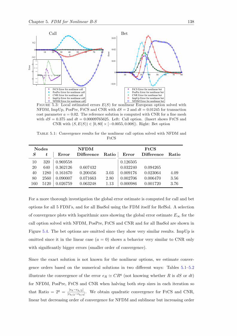
Chapter 5. FDM for Nonlinear B-S 138
BetCall
Figure 5.3: Local estimated errors E(S) for nonlinear European option solved withNFDM, ImpUp, PosPre, FtCS and CNR with dS = 2 and dt = 0.01245 for transactioncost parameter a = 0.02. The reference solution is computed with CNR for a fine meshwith dS = 0.375 and dt = 0.00009765625. Left: Call option. (Insert shows FtCS and
CNR with (S,E(S)) ∈ [0, 80]× [−0.0055, 0.008]). Right: Bet option
Table 5.1: Convergence results for the nonlinear call option solved with NFDM andFtCS
Nodes NFDM FtCSS t Error Difference Ratio Error Difference Ratio
10 320 0.969558 0.12650520 640 0.362126 0.607432 0.032240 0.09426540 1280 0.161670 0.200456 3.03 0.009176 0.023064 4.0980 2560 0.090007 0.071663 2.80 0.002706 0.006470 3.56160 5120 0.026759 0.063248 1.13 0.000986 0.001720 3.76
For a more thorough investigation the global error estimate is computed for call and bet
options for all 5 FDM’s, and for all BasSol using the FDM itself for RefSol. A selection
of convergence plots with logarithmic axes showing the global error estimate E∞ for the
call option solved with NFDM, PosPre, FtCS and CNR and for all BasSol are shown in
Figure 5.4. The bet options are omitted since they show very similar results. ImpUp is
omitted since it in the linear case (a = 0) shows a behavior very similar to CNR only
with significantly bigger errors (smaller order of convergence).
Since the exact solution is not known for the nonlinear options, we estimate conver-
gence orders based on the numerical solutions in two different ways: Tables 5.1–5.2
illustrate the convergence of the error eR ' CRq (not knowing whether R is dS or dt)
for NFDM, PosPre, FtCS and CNR when halving both step sizes in each iteration so
that Ratio = 2q =|eh−eh/2||eh/2−eh/4|
. We obtain quadratic convergence for FtCS and CNR,
linear but decreasing order of convergence for NFDM and sublinear but increasing order

Chapter 5. FDM for Nonlinear B-S 139
(a) log10(estimated NFDM error) (b) log10(estimated PosPre error)
(c) log10(estimated FtCS error) (d) log10(estimated CNR error)
Figure 5.4: Global estimated errors E∞ for nonlinear European Call options whensolved with NFDM (a), PosPre (b), FtCS (c) and CNR (d) for transaction cost param-eter a = 0.02 at time t = 0. The reference solution is computed with NFDM, PosPre,FtCS and CNR respectively for a fine mesh with dS = 0.375 and dt = 0.00009765625
Table 5.2: Convergence results for the nonlinear call option solved with CNR andPosPre
Nodes CNR PosPreS t Error Difference Ratio Error Difference Ratio
10 320 0.127837 0.07703520 640 0.032952 0.094885 0.075434 0.00160140 1280 0.009476 0.023476 4.04 0.065135 0.010299 0.1680 2560 0.002836 0.006640 3.53 0.040396 0.024739 0.42160 5120 0.001026 0.001810 3.66 0.011714 0.028682 0.86
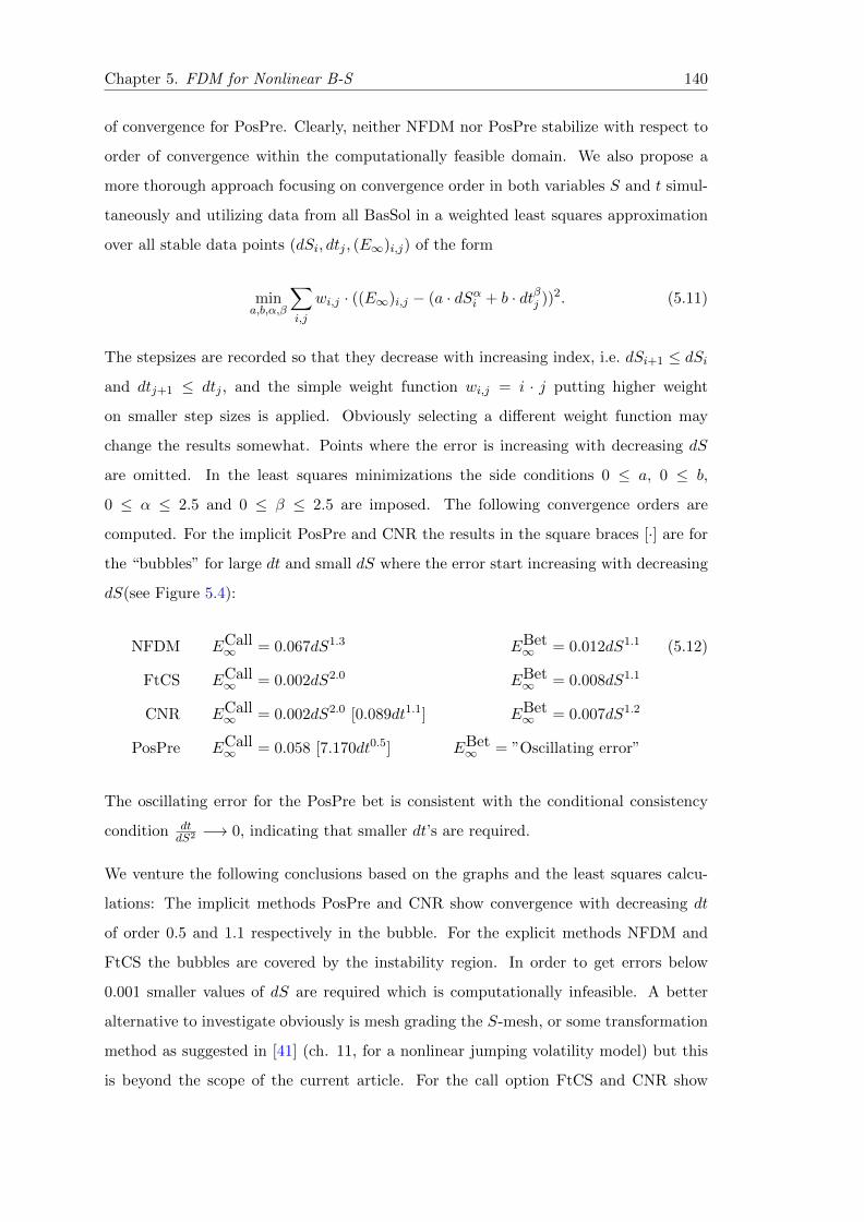
Chapter 5. FDM for Nonlinear B-S 140
of convergence for PosPre. Clearly, neither NFDM nor PosPre stabilize with respect to
order of convergence within the computationally feasible domain. We also propose a
more thorough approach focusing on convergence order in both variables S and t simul-
taneously and utilizing data from all BasSol in a weighted least squares approximation
over all stable data points (dSi, dtj , (E∞)i,j) of the form
mina,b,α,β
∑i,j
wi,j · ((E∞)i,j − (a · dSαi + b · dtβj ))2. (5.11)
The stepsizes are recorded so that they decrease with increasing index, i.e. dSi+1 ≤ dSi
and dtj+1 ≤ dtj , and the simple weight function wi,j = i · j putting higher weight
on smaller step sizes is applied. Obviously selecting a different weight function may
change the results somewhat. Points where the error is increasing with decreasing dS
are omitted. In the least squares minimizations the side conditions 0 ≤ a, 0 ≤ b,
0 ≤ α ≤ 2.5 and 0 ≤ β ≤ 2.5 are imposed. The following convergence orders are
computed. For the implicit PosPre and CNR the results in the square braces [·] are for
the “bubbles” for large dt and small dS where the error start increasing with decreasing
dS(see Figure 5.4):
NFDM ECall∞ = 0.067dS1.3 EBet
∞ = 0.012dS1.1 (5.12)
FtCS ECall∞ = 0.002dS2.0 EBet
∞ = 0.008dS1.1
CNR ECall∞ = 0.002dS2.0 [0.089dt1.1] EBet
∞ = 0.007dS1.2
PosPre ECall∞ = 0.058 [7.170dt0.5] EBet
∞ = ”Oscillating error”
The oscillating error for the PosPre bet is consistent with the conditional consistency
condition dtdS2 −→ 0, indicating that smaller dt’s are required.
We venture the following conclusions based on the graphs and the least squares calcu-
lations: The implicit methods PosPre and CNR show convergence with decreasing dt
of order 0.5 and 1.1 respectively in the bubble. For the explicit methods NFDM and
FtCS the bubbles are covered by the instability region. In order to get errors below
0.001 smaller values of dS are required which is computationally infeasible. A better
alternative to investigate obviously is mesh grading the S-mesh, or some transformation
method as suggested in [41] (ch. 11, for a nonlinear jumping volatility model) but this
is beyond the scope of the current article. For the call option FtCS and CNR show

Chapter 5. FDM for Nonlinear B-S 141
the expected quadratic convergence with dS outside the bubble whereas NFDM only
shows an order slightly above linear and PosPre shows no convergence at all. For the
bet option both FtCS, CNR and NFDM show orders of convergence in dS slightly above
linear. The stability area for FtCS is comparable to the one for NFDM (see Figure 5.2).
Comparing the methods clearly FtCS and CNR stand out above the rest, the choice
being whether to go for the fast computational times for the explicit FtCS, dealing with
the instability area increasing in size with the transaction cost parameter a and reducing
the usable area for the explicit methods to approximately 0 ≤ a ≤ 0.1, or whether to
accept the longer computational times of the implicit CNR, avoiding the concerns about
feasible dt–dS combinations for the implicit, absolutely stable CNR.
5.5 Conclusions
The “classical Explicit Euler” is the better explicit method and the “classical with
a twist Crank-Nicolson with Rannacher time stepping” is the better implicit method
among the FDM’s tested on the Barles and Soner nonlinear Black-Scholes model. The
non oscillating methods do not offer any enhancement of the performance in the cases
considered. The explicit methods suffer from an instability region growing with the
transaction cost parameter a rendering them somewhat useless for a ≥ 0.1. None of
the methods considered show significant convergence with dt — the error from the S-
direction dominating except for the coarsest time step sizes. Because of computer time
limitations the brute force solution (smaller dS) seems out of reach pointing instead
towards graded S-meshes as the obvious solution to get in the ideal zone where the
errors from t and S are balanced.


Appendix
5.A NFDM Scheme
The nonstandard finite difference scheme [NFDM] is based on an “exact finite difference
scheme” for the linear first order reaction and convection terms removing the diffusion
term by taking σ0 = 0. Then this scheme is applied to the complete problem only adding
nonstandard finite difference approximations of the diffusion term. So first we consider
the problem∂U
∂τ− rS ∂U
∂S+ rU = 0 for (S, τ) ∈ (0, Smax)× (0, T )
U(S, 0) = κ(S, T ) for S ∈ (0, Smax)
where κ(S, t) is the utility function defined in (5.3). The solution to this problem is
U(S, τ) = κ(Serτ , T )e−rτ and it is easily seen that this function satisfies
U(S, τ + ∆τ)− U(S, τ)
θ(∆τ)= −rU(S, τ)
where
θ(∆τ) =1− e−r∆τ
r= ∆τ +O(∆τ2)
and
S = Ser∆τ =S
1− rθ(∆τ)⇒ S − S = S
rθ(∆τ)
1− rθ(∆τ).
143

Chapter 5. Appendix 144
This is in the form of an “exact finite difference scheme” for the above linear equation.
By Taylor expansion using ∆τθ(∆τ) = 1 +O(∆τ) it is easily seen that (for any smooth U)
∂U
∂τ(S, τ)− rS ∂U
∂S(S, τ) + rU(S, τ) =
U(S, τ + ∆τ)− U(S, τ)
θ(∆τ)+ rU(S, τ) +O(∆τ).
(5.13)
Note that the approximation retains the order if θ(∆τ) is replaced by ∆τ .
In order to reach a useful finite difference scheme the solution in the ghost point S
is “split” between the two adjacent mesh points S and S + ∆S by Taylor expansion.
Arenas et el [2] use the following 1st order Taylor expansion:
U(S, τ) = U0∆S,∆τ (S, τ) +O(∆S∆τ + ∆τ2) where
U0∆S,∆τ (S, τ) = U(S, τ) + (S − S)
U(S + ∆S, τ)− U(S, τ)
∆S. (5.14)
Requiring S ≤ S ≤ S + ∆S ∀S ∈ [0, Smax] which is equivalent to the condition
Smax(er∆τ − 1) ≤ ∆S ⇔ ∆τ ≤ 1
r ln(1 + ∆SSmax
)≤ ∆S
rSmax+O(∆S2) (5.15)
we end up with the truncation error O(∆S2). Inserting U0∆S,∆τ (S, τ) instead of U(S, τ)
in (5.13) we get
∂U
∂τ(S, τ)− rS ∂U
∂S(S, τ) + rU(S, τ)
=U(S, τ + ∆τ)− U0
∆S,∆τ (S, τ)
θ(∆τ)+ rU0
∆S,∆τ (S, τ) +O(∆τ) +O(∆S)
=U(S, τ + ∆τ)− U(S, τ)
θ(∆τ)− rSU(S + ∆S, τ)− U(S, τ)
∆S+ rU(S, τ)
+O(∆τ) +O(∆S). (5.16)
Clearly, this does not lead to 2nd order consistency in S as claimed in [2]. The method
is only first order consistent in S as well as t. Following [34] Arenas et al then suggest
the approximation arising from
∂2U
∂S2(S, τ) =
U(S −∆S, τ)− 2U(S, τ) + U(S + ∆S, τ)
φ(∆S)+O(∆S2) where
φ(∆S) =1
r(e√r∆S − 2 + e−
√r∆S) = ∆S2 +O(∆S4) (5.17)

Chapter 5. Appendix 145
for the second derivatives (noting that ∆S2
φ(∆S) = 1 + O(∆S2)) whereas the remaining S
and τ in the diffusion term are left unaltered. Note that the approximation retains the
order if φ(∆S) is replaced by ∆S2. This results in the following approximation:
∂U
∂τ(S, τ)− rS ∂U
∂S(S, τ) + rU(S, τ)− 1
2σ2BS(T − τ, S, USS)S2∂
2U
∂S2(S, τ)
=U(S, τ + ∆τ)− U(S, τ)
θ(∆τ)− rSU(S + ∆S, τ)− U(S, τ)
∆S+ rU(S, τ)
−1
2σ2BS(T − τ, S, USS)S2U(S −∆S, τ)− 2U(S, τ) + U(S + ∆S, τ)
φ(∆S)
+O(∆τ) +O(∆S). (5.18)
Now consider a uniform mesh Sj = jh for j = 0, . . . ,M and τn = nk for n = 0, . . . , N
where the condition (5.15) takes the form TN = k ≤ 1
r ln(1 + hSmax
) = 1r ln(1 + 1
M ) or
N & rT ·M which is a very mild condition satisfied for sufficiently small time stepsizes
k. We use unj as our approximation to U(Sj , τn), U being the solution to (5.6–5.7). Also
introduce the following difference operators:
δ+τ u
nj =
un+1j − unj
k, δ+
τ unj =
un+1j − unjθ(k)
,
δ+S u
nj =
unj+1 − unjh
, δ0Su
nj =
unj+1 − unj−1
2h,
δ0SSu
nj =
unj+1 − 2unj + unj−1
h2, δ0
SSunj =
unj+1 − 2unj + unj−1
φ(h), δ0
SSunj =
unj+1 − 2un+1j + unj−1
h2.
Discarding the truncation error terms in (5.18) we arrive at the explicit nonstandard
finite difference scheme for (5.6–5.7) [NFDM]
δ+τ u
nj −
1
2σ2BS(T − τn, Sj , δ0
SSunj )S2δ0
SSunj − rSjδ+
S unj + runj = 0
for j = 1, . . . ,M − 1, n = 0, . . . , N − 1 (h =Smax
M, k =
T
N, N & rT ·M),
u0j = κ(jh, T ), un0 = κ(0, T − nk), unM = κ(Smax, T − nk)
for j = 1, . . . ,M − 1, n = 0, . . . , N. (5.19)
This is easily recognized as an explicit upwinding method except for the nonstandard
first order approximations to h and k in most of the derivatives. By construction and
by the boundedness and smoothness of U and its derivatives this scheme is first order

Chapter 5. Appendix 146
consistent in τ and S in any Lp-norm (also L∞) under the assumption that
Ψ(ernkκ2R(jh)2δ0SSU
nj )−Ψ(ernkκ2R(jh)2USS(jh, nk)) = O(h1+q) = O(∆S1+q)
for q = 0, 1 and any smooth U. (5.20)
q = 0 is required for NFDM using (5.14) whereas q = 1 is required for FtCS using (5.21)
below, where (5.20) results in second order consistency in S in any Lp norm. Note that
these orders of consistency are valid also if replacing θ(k) by k and φ(h) by h2.
Note that FtCS may actually be created from NFDM simply by splitting S between the
mesh points S−∆S and S+ ∆S instead of between S and S+ ∆S and hence replacing
(5.14) by
U(S, τ) = U1∆S,∆τ (S, τ) +O(∆S2∆τ + ∆τ2) where
U1∆S,∆τ (S, τ) = U(S, τ) + (S − S)
U(S + ∆S, τ)− U(S −∆S, τ)
2∆S(5.21)
still assuming (5.15). Combining (5.13) and (5.21) we get
∂U
∂τ(S, τ)− rS ∂U
∂S(S, τ) + rU(S, τ)
=U(S, τ + ∆τ)− U1
∆S,∆τ (S, τ)
θ(∆τ)+ rU1
∆S,∆τ (S, τ) +O(∆τ) +O(∆S2)
=U(S, τ + ∆τ)− U(S, τ)
θ(∆τ)− rSU(S + ∆S, τ)− U(S −∆S, τ)
2∆S+ rU(S, τ)
+O(∆τ) +O(∆S2). (5.22)
Note that also this approximation retains the order if θ(∆τ) is replaced by ∆τ . Using
(5.17) and replacing θ(∆τ) by ∆τ and φ(∆S) by ∆S2 without the loss of consistency
order we arrive at FtCS. Since ∆τ ≤ O(∆S) by (5.15) the practical difference between
the different orders of NFDM and FtCS needs to be investigated further.

Chapter 5. Appendix 147
Now we focus on NFDM and FtCS who may be rewritten in a unified fashion as follows
(q = 0 for NFDM and q = 1 for FtCS):
un+1j = (1− rθ(k))
unj +
rθ(k)
(1 + q)(1− rθ(k))j(unj+1 − unj−q)
+θ(k)
2σ2
0
(1 + Ψ(ernkκ2R(jh)2δ0
SSunj ))j2h2δ0
SSunj
for q = 0, 1, j = 1, . . . ,M − 1, n = 0, . . . , N − 1 (h =Smax
M, k =
T
N, N & rT ·M),
u0j = κ(jh, T ), un0 = κ(0, T − nk), unM = κ(Smax, T − nk)
for j = 1, . . . ,M − 1, n = 0, . . . , N. (5.23)
Note that Arenas et al [2] apply the boundary conditions ∂2U∂S2 = 0 in (0, τ) and (Smax, τ)
in hard form by δ0SSu
n0 = δ0
SSunM = 0 thus introducing the ghost points S−1 = −h and
SM+1 = Smax + h and at the same time extending the finite difference scheme (5.23) to
include also j = 0 and j = M . We shall do the same for our theoretical investigations
even though we for the practical computations are using the Dirichlet conditions from
(5.7) only approximately satisfying these conditions. By rearranging the terms (5.23)
can be written as
un+1j = anj u
nj+1 + bnj u
nj + cnj u
nj−1
for j = 1, . . . ,M − 1, n = 0, . . . , N − 1 and
u0j = κ(jh, T ), un0 = κ(0, T − nk), unM = κ(Smax, T − nk)
for j = 1, . . . ,M − 1, n = 0, . . . , N (h =Smax
M, k =
T
N, N & rT ·M) (5.24)
or with derivative boundary conditions
un+1j = anj u
nj+1 + bnj u
nj + cnj u
nj−1
for j = 0, . . . ,M, n = 0, . . . , N − 1 (h =Smax
M, k =
T
N, N & rT ·M) and
u0j = κ(jh, T ), δ0
SSun0 = δ0
SSunM = 0
for j = 0, . . . ,M, n = 0, . . . , N (h =Smax
M, k =
T
N, N & rT ·M) (5.25)

Chapter 5. Appendix 148
where
anj =rθ(k)j
1 + q+θ(k)ωnj2φ(h)
,
bnj = 1− rθ(k)
(1− q1 + q
j + 1
)−θ(k)ωnjφ(h)
,
cnj = −qrθ(k)j
1 + q+θ(k)ωnj2φ(h)
,
ωnj = σ20(jh)2
[1 + Ψ
(ernkκ2R(jh)2δ0
SSunj
)]= S2
j σ2BS(T − τn, Sj , δ0
SSunj ) ≥ 0
for q = 0, 1, j = 0, . . . ,M, n = 0, . . . , N (h =Smax
M, k =
T
N, N & rT ·M).(5.26)
Here q = 0 corresponds to NFDM while q = 1 corresponds to FtCS. The theoretical
properties of NFDM (and FtCS) are covered by Appendix 5.B
5.B NFDM Perperties Theorem
Theorem 5.1. If
θ(k)
(rM +
r2θ(k)M2
1− rθ(k)+
1
φ(h)max
j=0,...,Mn=0,...,N−1
ωnj
)≤ 1 (5.27)
(which will be satisfied for sufficiently small time stepsizes k) then
1. the nonstandard finite difference schemes (5.24) and (5.25) for q = 0 are nonneg-
ative, i.e. unj ≥ 0 for all j = 0, . . . ,M and n = 0, . . . , N .
2. the nonstandard finite difference scheme (5.25) for q = 0 is monotonicity preserv-
ing in S, i.e. unj+1 ≥ (≤) unj for all j = 0, . . . ,M − 1 and any n = 0, . . . , N − 1⇒
un+1j+1 ≥ (≤) un+1
j for all j = 0, . . . ,M − 1.
3. the nonstandard finite difference scheme (5.25) for q = 0 for the put option is
monotone nonincreasing with S, i.e. un0 ≥ . . . ≥ unM for all n = 0, . . . , N . For the
call and bet options the scheme is monotone nondecreasing with S, i.e. un0 ≤ . . . ≤
unM for all n = 0, . . . , N .
4. the nonstandard finite difference schemes (5.24) and (5.25) are consistent in any
Lp norm (p ∈ [1,∞]) of order 1 in τ and order 1 + q in S (for q = 0, 1) assuming
(5.20).

Chapter 5. Appendix 149
5. the nonstandard finite difference schemes (5.24) and (5.25) are stable in the L∞
norm (for q = 0, 1), i.e. ‖un‖∞ ≤ Ceβτn‖u0‖∞ for all n = 0, 1, . . . for some
C, β ≥ 0 where un = [un0 , . . . , unM ]T .
6. the nonstandard finite difference schemes (5.24) and (5.25) are convergent in the
L∞ norm of order 1 in τ and order 1 + q in S (for q = 0, 1) to the solution to
(5.6–5.7) assuming (5.20).
Proof.
1.
Here we provide the proof for the nonnegativity of (5.24), the details for (5.25) following
from the exposition in [19].
For all j = 1, . . . ,M −1, n = 0, . . . , N with initial data given by (5.24) and by definition
of the put, call and bet options, u0j ≥ 0, un0 ≥ 0 and unM ≥ 0. By (5.26) also anj ≥ 0 for
q = 0, 1 and cnj ≥ 0 for q = 0. In order to have cnj ≥ 0 also for q = 1 we would need
φ(h) ≤ 1
rMmin
j=0,...,Mn=0,...,N−1
ωnj for q = 1 (5.28)
but since ωnj ' 0 close to the S-boundaries, this condition is not satisfied. Hence FtCS
cannot be shown to be nonnegative by this method, which is consistent with the practical
observations that FtCS may oscillate near S = Smax but does not oscillate near S = K.
If only bnj ≥ 0 for j = 1, . . . ,M − 1, n = 0, . . . , N − 1, (5.24) implies that unj ≥ 0 for
j = 0, . . . ,M , n = 0, . . . , N , i.e. the scheme is nonnegative.
The nonnegativity of bnj hinges on the properties of δnj and the function Ψ and is here
only stated in general terms as the assumption (5.27).
Obviously (5.27) ⇒ minj=1,...,M−1n=0,...,N−1
(1− rθ(k)
(1−q1+q j + 1
)− qr2θ(k)2j2
1−rθ(k) −θ(k)φ(h)ω
nj
)≥ 0⇔
minj=1,...,M−1n=0,...,N−1
bnj ≥ 0.
2.
Let us consider only the nondecreasing case, since the nonincreasing case is identical
apart from the orientation of the inequality signs. Hence assume that
unj+1 ≥ unj for all j = 0, . . . ,M − 1 and any n = 0, . . . , N − 1. (5.29)
Note that δn0 = 0 ⇔ un−1 = 2un0 − un1 = un0 + (un0 − un1 )(5.29)
≤ un0 . Hence (5.29) can be
extended to j = −1.

Chapter 5. Appendix 150
Also δnM = 0⇔ unM+1 = 2unM − unM−1 = unM + (unM − unM−1)(5.29)
≥ unM . Hence (5.29) can
be extended to j = M .
Thus we have
unj+1 ≥ unj for all j = −1, . . . ,M and some n = 0, . . . , N − 1. (5.30)
Also note that by simple computation from (5.26)
anj + (bnj + rθ(k)) + cnj = 1 for all j = 0, . . . ,M. (5.31)
For j = 0, . . . ,M − 1:
un+1j − unj
(5.24)= anj u
nj+1 + bnj u
nj + cnj u
nj−1 − unj
(5.30)
≤ anj unj+1 + bnj u
nj + cnj u
nj − unj
= anj (unj+1 − unj ) + (anj + bnj + cnj − 1)unj(5.31)
= anj (unj+1 − unj )− rθ(k)unj
and
un+1j+1 − unj+1
(5.24)= anj+1u
nj+2 + bnj+1u
nj+1 + cnj+1u
nj − unj+1
(5.30)
≥ anj+1unj+1 + bnj+1u
nj+1 +
cnj+1unj − unj+1
= −cnj+1(unj+1 − unj ) + (cnj+1 + anj+1 + bnj+1 − 1)unj+1
(5.31)= −cnj+1(unj+1 − unj )− rθ(k)unj+1.
and hence
un+1j+1−u
n+1j = (un+1
j+1−unj+1)+(unj+1−unj )−(un+1j −unj ) ≥
(−cnj+1 + 1− anj − rθ(k)
)(unj+1 − unj
)≥ 0 where the last term is nonnegative by (5.30) and the first term is nonnegative by
(5.27) and the following argument:
−cnj+1 + 1− anj − rθ(k)(5.26)
= − θ(k)2φ(h)ω
nj+1 + 1− rjθ(k)− θ(k)
2φ(h)ωnj + 1− rθ(k)
= 1−r(j+1)θ(k)− θ(k)2φ(h)(ωnj +ωnj+1) ≥ 1−rMθ(k)− θ(k)
2φ(h)(maxj=0,...,M−1 ωnj +maxj+1=1,...,M ωnj+1)
≥ 1− rMθ(k)− θ(k)φ(h) max j=0,...,M
n=0,...,N−1ωnj
(5.27)
≥ 0.
3.
For the put option, u0j+1 ≤ u0
j for all j = 0, . . . ,M − 1.
For the call and bet options u0j+1 ≥ u0
j for all j = 0, . . . ,M − 1.
The results then follow from monotonicity preservation.
4.
For (5.24) see below (5.19). The consistency in the L∞ norm for (5.25) follows from the
exposition in [19] and the general Lp-norm is a simple generalization.
5.
Here we provide the proof for the stability of (5.24), the details for (5.25) following from
the exposition in [19].

Chapter 5. Appendix 151
First un0 = [0∨Ke−rτ ∨0] ≤ [0∨K∨0] = u00 ≤ ‖u0‖∞ satisfying the stability requirement
with C = 1 and β = 0.
Also unM = [Smax −Ke−rτ ∨ 0 ∨Be−rτ ] ≤ [Smax−Ke−rτSmax−K (Smax −K) ∨ 0 ∨B] ≤ [α(Smax −
K) ∨ 0 ∨ B] ≤ maxα, 1u00 ≤ maxα, 1‖u0‖∞ where α = Smax−Ke−rT
Smax−K ≥ Smax−Ke−rτSmax−K .
Hence the stability requirement is satisfied with C = maxα, 1 and β = 0.
Finally for j = 1, . . . ,M − 1:
un+1j
(5.24)= anj u
nj+1 + bnj u
nj + cnj u
nj−1 ≤ (anj + bnj + cnj )‖un‖∞
where 0 ≤ anj + bnj + cnj(5.31)
= 1− rθ(k) ≤ 1 so that un+1j ≤ ‖un‖∞ ⇒ unj ≤ ‖u0‖∞ which
satisfies the stability requirement with C = 1 and β = 0.
In conclusion ‖un‖∞ ≤ C‖u0‖∞ where C = maxα, 1.
6.
This follows from Lax’s convergence theorem and bullets 4 and 5.
5.C Ψ(x) Plot
A plot of Ψ is shown in Figure 5.C.1.
Figure 5.C.1: The Barles and Soner Ψ function satisfying (5.5).


Bibliography
[1] J. Ankudinova and M. Ehrhardt, On the numerical solution of nonlinear black–
scholes equations, Computers & Mathematics with Applications, 56 (2008), pp. 799–
812.
[2] A. J. Arenas, G. Gonzalez-Parra, and B. M. Caraballo, A nonstandard
finite difference scheme for a nonlinear black–scholes equation, Mathematical and
Computer Modelling, 57 (2013), pp. 1663–1670.
[3] D. Bakstein and S. Howison, A non-arbitrage liquidity model with observable
parameters for derivatives, Mathematical Finance, (2003).
[4] G. Barles and H. M. Soner, Option pricing with transaction costs and a non-
linear black-scholes equation, Finance and Stochastics, 2 (1998), pp. 369–397.
[5] F. Black and M. Scholes, The pricing of options and corporate liabilities, The
journal of political economy, (1973), pp. 637–654.
[6] P. P. Boyle and T. Vorst, Option replication in discrete time with transaction
costs, The Journal of Finance, 47 (1992), pp. 271–293.
[7] M. J. Brennan and E. S. Schwartz, Finite difference methods and jump pro-
cesses arising in the pricing of contingent claims: A synthesis, Journal of Financial
and Quantitative Analysis, 13 (1978), pp. 461–474.
[8] R. Company, L. Jodar, and J. R. Pintos, A numerical method for european op-
tion pricing with transaction costs nonlinear equation, Mathematical and Computer
Modelling, 50 (2009), pp. 910–920.
[9] R. Cont and E. Voltchkova, A finite difference scheme for option pricing in
jump diffusion and exponential levy models, SIAM Journal on Numerical Analysis,
43 (2005), pp. 1596–1626.
153

Bibliography 154
[10] D. J. Duffy, A critique of the crank nicolson scheme strengths and weaknesses
for financial instrument pricing, 70+ DVDs FOR SALE & EXCHANGE, (2004),
p. 333.
[11] , Finite Difference methods in financial engineering: a Partial Differential
Equation approach, John Wiley & Sons, 2006.
[12] M. Ehrhardt, Nonlinear models in mathematical finance: new research trends in
option pricing, Nova Science Publishers, 2008.
[13] P. A. Forsyth and G. Labahn, Numerical methods for controlled hamilton-
jacobi-bellman pdes in finance, Journal of Computational Finance, 11 (2007), p. 1.
[14] R. Frey, Market illiquidity as a source of model risk in dynamic hedging, in Model
Risk, Risk Publications, London, 2000, pp. 125–136.
[15] R. Frey and P. Patie, Risk management for derivatives in illiquid markets: A
simulation study, in Advances in finance and stochastics, Springer, 2002, pp. 137–
159.
[16] R. Frey and A. Stremme, Market volatility and feedback effects from dynamic
hedging, Mathematical finance, 7 (1997), pp. 351–374.
[17] M. B. Giles and R. Carter, Convergence analysis of crank-nicolson and ran-
nacher time-marching, (2005).
[18] K. J. Glover, The analysis of PDEs arising in nonlinear and non-standard option
pricing, PhD thesis, University of Manchester, 2008.
[19] G. Gonzalez-Parra, A. J. Arenas, and B. M. Chen-Charpentier, Positive
numerical solution for a nonarbitrage liquidity model using nonstandard finite dif-
ference schemes, Numerical Methods for Partial Differential Equations, 30 (2014),
pp. 210–221.
[20] E. G. Haug, The complete guide to option pricing formulas, vol. 2, McGraw-Hill
New York, 1998.
[21] T. Hoggard, A. E. Whalley, and P. Wilmott, Hedging option portfolios in
the presence of transaction costs, Advances in Futures and Options Research, 7
(1994), pp. 21–35.

Bibliography 155
[22] M. H. Holmes, Introduction to numerical methods in differential equations, vol. 52,
Springer, 2007.
[23] J. Hugger, The boundary value formulation of the asian call option, in Numerical
Mathematics and Advanced Applications, Springer, 2003, pp. 409–418.
[24] , Wellposedness of the boundary value formulation of a fixed strike asian option,
Journal of computational and applied mathematics, 185 (2006), pp. 460–481.
[25] M. Jandacka and D. Sevcovic, On the risk-adjusted pricing-methodology-based
valuation of vanilla options and explanation of the volatility smile, Journal of Ap-
plied Mathematics, 2005 (2005), pp. 235–258.
[26] R. Korn and E. Korn, Option pricing and portfolio optimization, American
Math. Soc., Providence, (2001).
[27] M. Kratka, No mystery behind the smile, Risk, 9 (1998), pp. 67–71.
[28] P. Kutik and K. Mikula, Finite volume schemes for solving nonlinear partial
differential equations in financial mathematics, in Finite Volumes for Complex Ap-
plications VI Problems & Perspectives, Springer, 2011, pp. 643–651.
[29] Y.-K. Kwok, Mathematical models of financial derivatives, Springer, 2008.
[30] H. E. Leland, Option pricing and replication with transactions costs, The journal
of finance, 40 (1985), pp. 1283–1301.
[31] D. C. Lesmana and S. Wang, An upwind finite difference method for a nonlinear
black–scholes equation governing european option valuation under transaction costs,
Applied Mathematics and Computation, (2013).
[32] H. Liu and J. Yong, Option pricing with an illiquid underlying asset market,
Journal of Economic Dynamics and Control, 29 (2005), pp. 2125–2156.
[33] R. C. Merton et al., Theory of rational option pricing, (1971).
[34] R. E. Mickens, Nonstandard finite difference models of differential equations,
World Scientific, 1994.
[35] E. Navarro, J. R. Pintos, E. Ponsoda, et al., Numerical solution of linear
and nonlinear black–scholes option pricing equations, Computers & Mathematics
with Applications, 56 (2008), pp. 813–821.

Bibliography 156
[36] C. W. Oosterlee, C. C. W. Leentvaar, and X. Huang, Accurate ameri-
can option pricing by grid stretching and high order finite differences, tech. report,
Working papers, DIAM, Delft University of Technology, the Netherlands, 2005.
[37] O. Østerby, Five ways of reducing the crank–nicolson oscillations, BIT Numerical
Mathematics, 43 (2003), pp. 811–822.
[38] D. M. Pooley, K. R. Vetzal, and P. A. Forsyth, Convergence remedies for
non-smooth payoffs in option pricing, Journal of Computational Finance, 6 (2003),
pp. 25–40.
[39] R. Rannacher, Finite element solution of diffusion problems with irregular data,
Numerische Mathematik, 43 (1984), pp. 309–327.
[40] C. Reisinger and A. Whitley, The impact of a natural time change on the
convergence of the crank–nicolson scheme, IMA Journal of Numerical Analysis,
(2013), p. drt029.
[41] D. Sevcovic, B. Stehlıkova, and K. Mikula, Analytical and numerical meth-
ods for pricing financial derivatives, Nova Science Publ. ISBN, (2011), pp. 978–1.
[42] R. Seydel, Tools for computational finance, Springer, 2012.
[43] D. Y. Tangman, A. Gopaul, and M. Bhuruth, Numerical pricing of options
using high-order compact finite difference schemes, Journal of Computational and
Applied Mathematics, 218 (2008), pp. 270–280.
[44] D. Tavella and C. Randall, Pricing financial instruments: The finite difference
method, John Wiley & Sons New York, 2000.
[45] J. Wang and P. A. Forsyth, Maximal use of central differencing for hamilton-
jacobi-bellman pdes in finance, SIAM Journal on Numerical Analysis, 46 (2008),
pp. 1580–1601.
[46] P. Wilmott, The mathematics of financial derivatives: a student introduction,
Cambridge University Press, 1995.
[47] Y. Zhao and W. T. Ziemba, On leland’s option hedging strategy with transaction
costs, tech. report, Humboldt University, Berlin, Germany, 2003.

Bibliography 157
[48] S. Zhou, W. Li, Y. Wei, and C. Wen, A positivity-preserving numerical scheme
for nonlinear option pricing models, Journal of Applied Mathematics, 2012 (2012).