numerical methods for first order odes

1.723 - COMPUTATIONAL METHODS FOR FLOW IN POROUS MEDIASpring 2009

NUMERICAL METHODS FOR FIRST ORDER ODEs

Luis Cueto-Felgueroso

1. PROBLEM STATEMENT

Consider a system of first order ordinary differential equations of the form

duuuuuuuuuuuuuu

dt= ffffffffffffff(t, uuuuuuuuuuuuuu), 0 ≤ t ≤ T, uuuuuuuuuuuuuu(t = 0) = uuuuuuuuuuuuuu0, (1)

whereuuuuuuuuuuuuuu andffffffffffffff are vectors withN components,uuuuuuuuuuuuuu = uuuuuuuuuuuuuu(t), andffffffffffffff is in general a nonlinear function oftanduuuuuuuuuuuuuu. Whenffffffffffffff does not depend explicitly ont, we say that the system (1) is autonomous. We discretizethe time domaint ∈ [0, T ] as

0 = t0 < t1 < . . . < tn < . . . < tM−1 < tM = T, (2)

and seek numerical methods that approximateuuuuuuuuuuuuuu at at times{tn, n = 0, . . . , M}, in the sense that

uuuuuuuuuuuuuun ≈ uuuuuuuuuuuuuu(t = tn), (3)

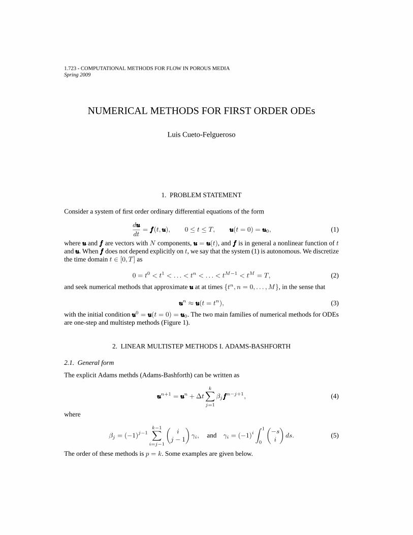
with the initial conditionuuuuuuuuuuuuuu0 = uuuuuuuuuuuuuu(t = 0) = uuuuuuuuuuuuuu0. The two main families of numerical methods for ODEsare one-step and multistep methods (Figure 1).

2. LINEAR MULTISTEP METHODS I. ADAMS-BASHFORTH

2.1. General form

The explicit Adams methds (Adams-Bashforth) can be written as

uuuuuuuuuuuuuun+1 = uuuuuuuuuuuuuun + ∆t

k∑

j=1

βjffffffffffffffn−j+1, (4)

where

βj = (−1)j−1k−1∑

i=j−1

(i

j − 1

)γi, and γi = (−1)i

∫ 1

0

(−si

)ds. (5)

The order of these methods isp = k. Some examples are given below.

2 NUMERICAL METHODS FOR ODES

tn

tn+1

Un

U1

U2

Un+1

tn−2

tn−1

tn

tn+1

Figure 1. Schematic of solution update in one-step (left) and multistep (right) methods.

2.1.1. k=1 (Forward Euler)

uuuuuuuuuuuuuun+1 = uuuuuuuuuuuuuun + ∆tffffffffffffffn (6)

2.1.2. k=2

uuuuuuuuuuuuuun+1 = uuuuuuuuuuuuuun +∆t

2(3ffffffffffffffn − ffffffffffffffn−1

)(7)

2.1.3. k=3


12(23ffffffffffffffn − 16ffffffffffffffn−1 + 5ffffffffffffffn−2

)(8)

2.1.4. k=4


24(55ffffffffffffffn − 59ffffffffffffffn−1 + 37ffffffffffffffn−2 − 9ffffffffffffffn−3

)(9)

3. LINEAR MULTISTEP METHODS II. ADAMS-MOULTON

3.1. General form

The implicit Adams methods (Adams-Moulton) can be written as


k∑

j=0

βjffffffffffffffn−j+1. (10)

The order of these schemes isp = k + 1. Some examples are given below.

3.1.1. k=0 (Backward Euler)

uuuuuuuuuuuuuun+1 = uuuuuuuuuuuuuun + ∆tffffffffffffffn+1 (11)

1.723 - Computational methods for flow in porous media

LCF 3

3.1.2. k=1 (Trapezoidal rule)


2(ffffffffffffffn+1 + ffffffffffffffn

)(12)

3.1.3. k=2


12(5ffffffffffffffn+1 + 8ffffffffffffffn − ffffffffffffffn−1

)(13)

3.1.4. k=3


24(9ffffffffffffffn+1 + 19ffffffffffffffn − 5ffffffffffffffn−1 + ffffffffffffffn−2

)(14)

3.1.5. k=4


720(251ffffffffffffffn+1 + 646ffffffffffffffn − 264ffffffffffffffn−1 + 106ffffffffffffffn−2 − 19ffffffffffffffn−3

)(15)

4. LINEAR MULTISTEP METHODS III. BACKWARD DIFFERENTIATION

The Backward Differentiation Formulas (BDF) are implicit methods, based on one-sided differencesthat approximateduuuuuuuuuuuuuu/dt directly. The general form is

k∑

i=0

αiuuuuuuuuuuuuuun−i+1 = ∆tβ0ffffffffffffff

n+1. (16)

The order of these schemes isp = k. Some examples are given below.

4.0.6. BDF1, k= 1 (Backward Euler)

uuuuuuuuuuuuuun+1 − uuuuuuuuuuuuuun = ∆tffffffffffffffn+1 (17)

4.0.7. BDF2, k= 2

uuuuuuuuuuuuuun+1 − 43uuuuuuuuuuuuuun +

13uuuuuuuuuuuuuun−1 = ∆t

23ffffffffffffffn+1 (18)

4.0.8. BDF3, k= 3

uuuuuuuuuuuuuun+1 − 1811

uuuuuuuuuuuuuun +911

uuuuuuuuuuuuuun−1 − 211

uuuuuuuuuuuuuun−2 = ∆t611

ffffffffffffffn+1 (19)



5. ONE-STEP METHODS: RUNGE-KUTTA METHODS

5.1. General definition

One step of ans-stage Runge-Kutta scheme can be written as


s∑

i=1

bikkkkkkkkkkkkkki, kkkkkkkkkkkkkki = ffffffffffffff (tn + ci∆t, uuuuuuuuuuuuuui) , (20)

with stage values

uuuuuuuuuuuuuui = uuuuuuuuuuuuuun + ∆t

s∑

j=1

aijkkkkkkkkkkkkkkj . (21)

In the above expressions,∆t is the time step, andAAAAAAAAAAAAAA = {aij} ∈ Rs×s, bbbbbbbbbbbbbb ∈ Rs andcccccccccccccc ∈ Rs are thecharacteristic coefficients of each given Runge-Kutta scheme, which can be compactly written usingthe so-called Butcher tableau

c1 a11 a12 · · · a1s

c2 a21 a22 · · · a2s

......

.... ..

...cs as1 as2 · · · ass

b1 b2 · · · bs

b1 b2 · · · bs

The consistency vectorcccccccccccccc defines the points (in time) at which the method computes approximationsto the initial value problem, so that the stage values can be seen asuuuuuuuuuuuuuui ≈ uuuuuuuuuuuuuu (tn + ci∆t). The row sumcondition

ci =s∑

j=1

aij , ∀i = 1, . . . , s, (22)

is usually adopted to simplify the order conditions for high-order methods. Explicit schemes arecharacterized by{aij = 0, ∀j ≥ i}. The second set of coefficients{bi, i = 1, . . . , s} corresponds tothe embedded scheme, which is used for error estimation. Thus, a second approximationuuuuuuuuuuuuuun+1 can bedefined using the same coefficientsAAAAAAAAAAAAAA = {aij} ∈ Rs×s, andcccccccccccccc ∈ Rs, and stage valuesuuuuuuuuuuuuuui, i = 1, . . . , s,as


s∑

i=1

bikkkkkkkkkkkkkki, kkkkkkkkkkkkkki = ffffffffffffff (tn + ci∆t, uuuuuuuuuuuuuui) . (23)

The difference betweenuuuuuuuuuuuuuun+1 and uuuuuuuuuuuuuun+1 gives an estimate of the error incurred by the numericalapproximation, thus providing a criterion for time step adaptivity.


LCF 5

5.2. Diagonally implicit schemes

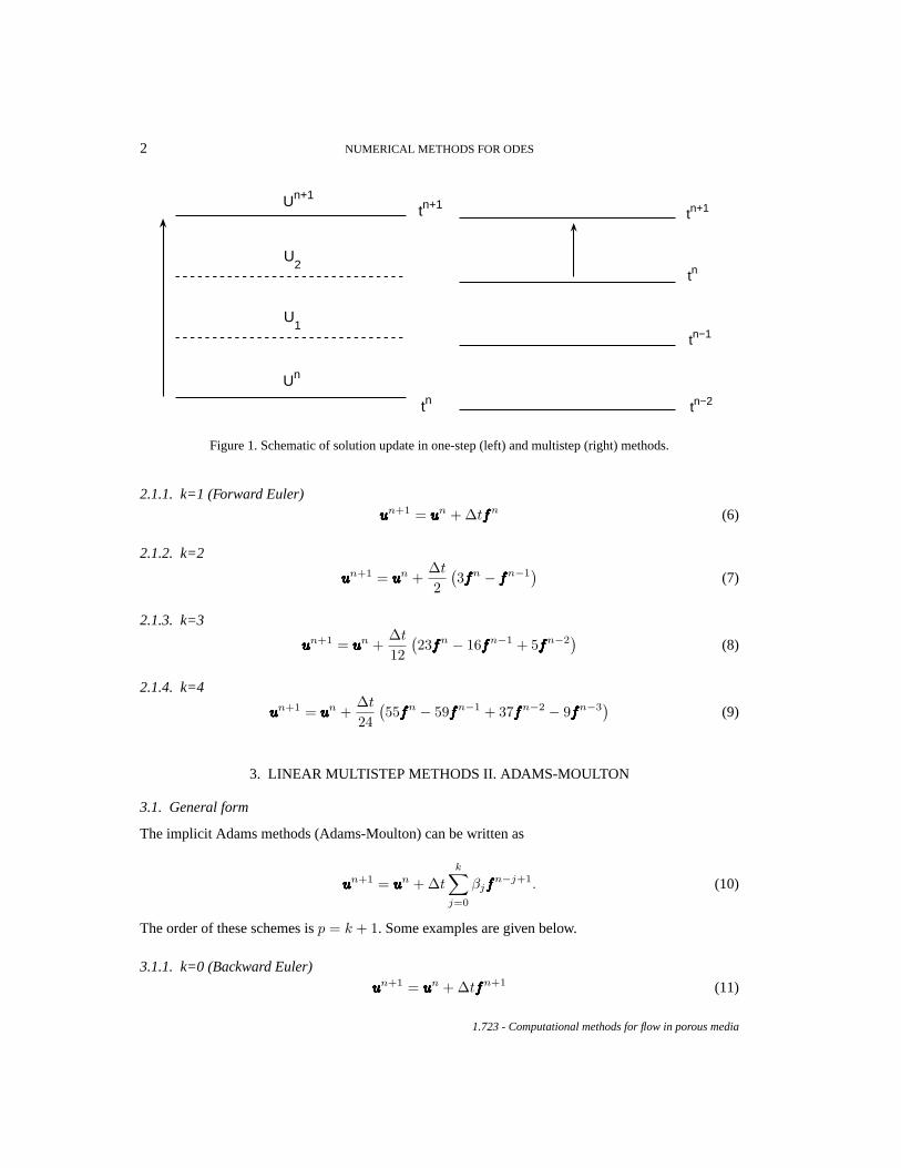
Among implicit RK schemes, the most popular ones for the time integration of PDEs are diagonallyimplicit. Their Butcher’s tableaux typically take the form

0 0 0 0 · · · 02γ γ γ 0 · · · 0c3 a31 a32 γ · · · 0...

......

.... ..

...1 as,1 as,2 as,3 · · · γ

b1 b2 b3 · · · γ

b1 b2 b3 · · · bs

In particular, these schemes are referred to asExplicit first step, Single diagonal coefficient,Diagonally Implicit Runge-Kutta(ESDIRK) methods. Each stage value of an ESDIRK scheme is atleast second-order accurate.

5.2.1. Implementation The stage value computation in a DIRK scheme reads


i∑

j=1

aij kkkkkkkkkkkkkkj (24)

Given that thei− 1 previouskkkkkkkkkkkkkk’s have been previously computed, (24) can be written as

uuuuuuuuuuuuuui = EEEEEEEEEEEEEEi + ∆taii kkkkkkkkkkkkkki, EEEEEEEEEEEEEEi = uuuuuuuuuuuuuun + ∆t

i−1∑

j=1

aij kkkkkkkkkkkkkkj (25)

The above expression is, in general, a nonlinear system of equations. Thep + 1 Newton iterationassociated to (25) is given by

(IIIIIIIIIIIIII −∆taii

∂kkkkkkkkkkkkkki

∂uuuuuuuuuuuuuu

∣∣∣∣p)

∆∆∆∆∆∆∆∆∆∆∆∆∆∆puuuuuuuuuuuuuui = EEEEEEEEEEEEEEi + ∆taii kkkkkkkkkkkkkkpi (26)

where∆∆∆∆∆∆∆∆∆∆∆∆∆∆puuuuuuuuuuuuuui = uuuuuuuuuuuuuup+1i − uuuuuuuuuuuuuup

i .The embedded scheme uses the same raw information as the original one, but in this case it is

“processed” using the second set of weights,{bi, i = 1, . . . , s}. Thus, at the end of each step of theRK integrator, we have


s∑

i=1

bikkkkkkkkkkkkkki uuuuuuuuuuuuuun+1 = uuuuuuuuuuuuuun + ∆t

s∑

i=1

bikkkkkkkkkkkkkki (27)

and the error estimate is given by some suitable norm of the difference between these two solutions,rn+1 = ||uuuuuuuuuuuuuun+1 − uuuuuuuuuuuuuun+1||.



5.3. Additive Runge-Kutta schemes: implicit-explicit (IMEX)

Consider systems of ordinary differential equations that can be written in additive form as

duuuuuuuuuuuuuu

dt=

N∑ν=1

ffffffffffffff [ν] (t, uuuuuuuuuuuuuu) (28)

whereffffffffffffff [1], ffffffffffffff [2], . . . , ffffffffffffff [N ] denote certain terms orcomponentsof ffffffffffffff , whose distinctive properties areworth being taken into account separately. The above expression (28) is in principle quite loosein terms of the considerations that lead to such splitting. In general, it may be advantageous toexploit the additive structure of the system (28) when eitherffffffffffffff or the unknownsuuuuuuuuuuuuuu themselves presentcomponents with significantly different time scales. In our PDE numerical solution context, the formercase typically corresponds to stiff-nonstiffa priori decompositions of the equations, whereas the lattercould apply to grid-induced stiffness. The idea behind additive schemes is to use, for each component,the integrator that best suits its particular characteristics.

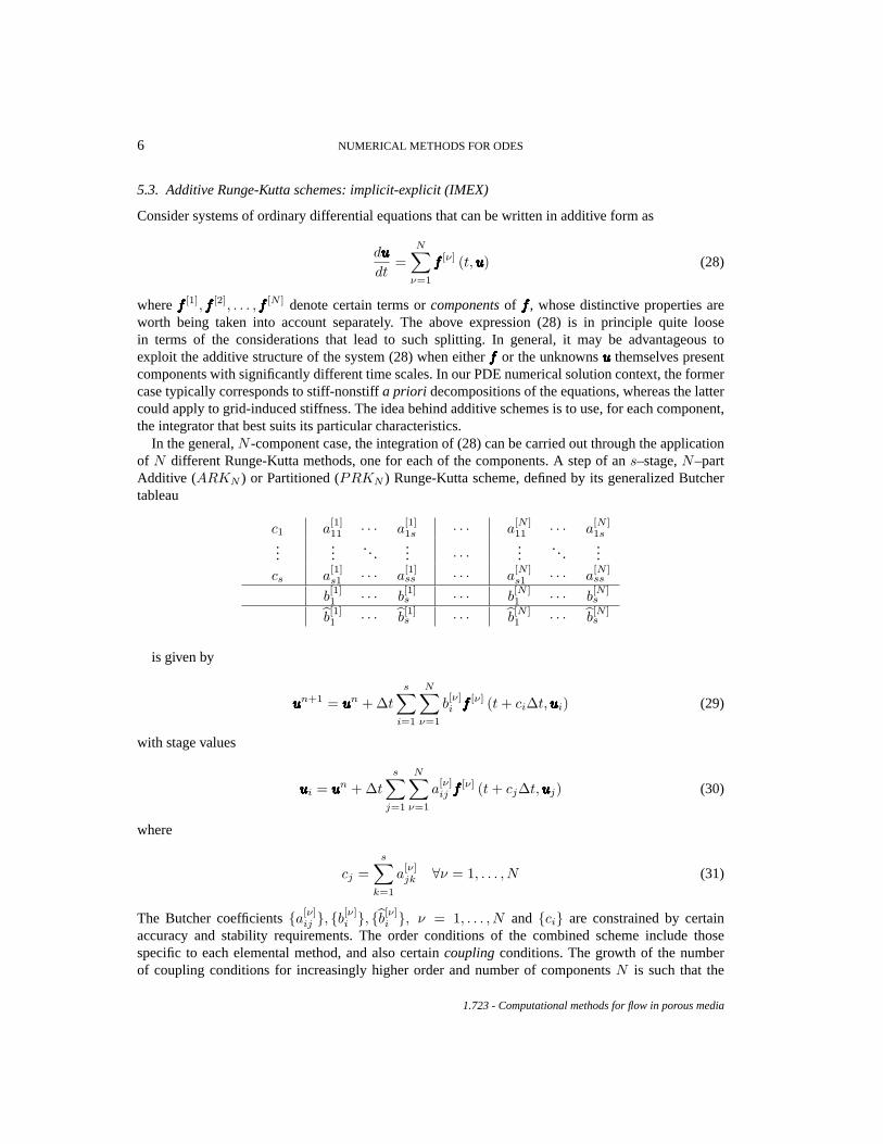
In the general,N -component case, the integration of (28) can be carried out through the applicationof N different Runge-Kutta methods, one for each of the components. A step of ans–stage,N–partAdditive (ARKN ) or Partitioned (PRKN ) Runge-Kutta scheme, defined by its generalized Butchertableau

c1 a[1]11 · · · a

[1]1s · · · a

[N ]11 · · · a

[N ]1s

......

. . .... · · · ...

. . ....

cs a[1]s1 · · · a

[1]ss · · · a

[N ]s1 · · · a

[N ]ss

b[1]1 · · · b

[1]s · · · b

[N ]1 · · · b

[N ]s

b[1]1 · · · b

[1]s · · · b

[N ]1 · · · b

[N ]s

is given by


s∑

i=1

N∑ν=1

b[ν]i ffffffffffffff [ν] (t + ci∆t, uuuuuuuuuuuuuui) (29)

with stage values


s∑

j=1

N∑ν=1

a[ν]ij ffffffffffffff [ν] (t + cj∆t, uuuuuuuuuuuuuuj) (30)

where

cj =s∑

k=1

a[ν]jk ∀ν = 1, . . . , N (31)

The Butcher coefficients{a[ν]ij }, {b[ν]

i }, {b[ν]i }, ν = 1, . . . , N and {ci} are constrained by certain

accuracy and stability requirements. The order conditions of the combined scheme include thosespecific to each elemental method, and also certaincouplingconditions. The growth of the numberof coupling conditions for increasingly higher order and number of componentsN is such that the


LCF 7

practical design ofARKN methods has been typically restricted toN = 2 (ARK2). In this latter case,the system (28) is conceptually written as

duuuuuuuuuuuuuu

dt= ffffffffffffffs (t, uuuuuuuuuuuuuu) + ffffffffffffffns (t, uuuuuuuuuuuuuu) (32)

where the right hand side of (28) has been generically split intostiff (ffffffffffffffs) andnonstiff (ffffffffffffffns) terms.Two different Runge-Kutta schemes, specifically designed and coupled, are applied to each term,and the important case in our context is theimplicit-explicit (IMEX) approach, which acknowledgesthe fact that the stiff part is more efficiently dealt with by means of animplicit integrator, whereasthe nonstiff part can be straightforwardly integrated using anexplicit scheme. In particular, manyproblems of practical interest are modeled by partial differential equations whose semidiscretizationcan be expressed in the form of (32), whereffffffffffffffs (t,UUUUUUUUUUUUUU) is linear but stiff, andffffffffffffffns (t,UUUUUUUUUUUUUU) is nonlinear butnonstiff. The resulting system of ODE’s can be very efficiently integrated using theIMEX approach.The combined integrators are referred to asIMEX ARK2 methods or, when the stiff terms are linear,linearly implicit Runge-Kutta schemes.

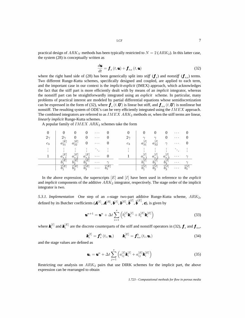
A popular family ofIMEX ARK2 schemes take the form

0 0 0 0 · · · 02γ 2γ 0 0 · · · 0

c3 a[E]31 a

[E]32 0 · · · 0

......

......

. . ....

1 a[E]s,1 a

[E]s,2 a

[E]s,3 · · · 0

b[E]1 b

[E]2 b

[E]3 · · · γ

b[E]1 b

[E]2 b

[E]3 · · · b

[E]s

0 0 0 0 · · · 02γ γ γ 0 · · · 0

c3 a[I]31 a

[I]32 γ · · · 0

......

......

.. ....

1 a[I]s,1 a

[I]s,2 a

[I]s,3 · · · γ

b[I]1 b

[I]2 b

[I]3 · · · γ

b[I]1 b

[I]2 b

[I]3 · · · b

[I]s

In the above expression, the superscripts[E] and [I] have been used in reference to theexplicitandimplicit components of the additiveARK2 integrator, respectively. The stage order of the implicitintegrator is two.

5.3.1. Implementation One step of ans-stage two-part additive Runge-Kutta scheme,ARK2,

defined by its Butcher coefficients (AAAAAAAAAAAAAA[I], AAAAAAAAAAAAAA[R], bbbbbbbbbbbbbb[I], bbbbbbbbbbbbbb[E], bbbbbbbbbbbbbb[I]

, bbbbbbbbbbbbbb[E]

, cccccccccccccc), is given by


s∑

i=1

(b[I]i kkkkkkkkkkkkkk

[I]i + b

[E]i kkkkkkkkkkkkkk

[E]i

)(33)

wherekkkkkkkkkkkkkk[I]i andkkkkkkkkkkkkkk

[E]i are the discrete counterparts of the stiff and nonstiff operators in (32),ffffffffffffffs andffffffffffffffns,

kkkkkkkkkkkkkk[I]i = ffffffffffffffh

s (ti, uuuuuuuuuuuuuui) kkkkkkkkkkkkkk[E]i = ffffffffffffffh

ns (ti, uuuuuuuuuuuuuui) (34)

and the stage values are defined as


s∑

j=1

(a[I]ij kkkkkkkkkkkkkk

[I]i + a

[E]ij kkkkkkkkkkkkkk

[E]i

)(35)

Restricting our analysis onARK2 pairs that use DIRK schemes for the implicit part, the aboveexpression can be rearranged to obtain




i−1∑

j=1


[I]j + a


[E]j

)+ ∆ta

[I]ii kkkkkkkkkkkkkk

[I]i (36)

We are interested in the linearly implicit case, for which the above expression is a linear system ofequations of the form

(IIIIIIIIIIIIII −∆ta

[I]ii KKKKKKKKKKKKKK

)uuuuuuuuuuuuuui = uuuuuuuuuuuuuun + ∆t

i−1∑

j=1


[I]j + a


[E]j

)(37)

wherekkkkkkkkkkkkkk[I]i = KKKKKKKKKKKKKKuuuuuuuuuuuuuui. After solving uuuuuuuuuuuuuui from (37), we can computekkkkkkkkkkkkkk[I]

i = ffffffffffffffs (ti, uuuuuuuuuuuuuui), andkkkkkkkkkkkkkk[E]i =

ffffffffffffffns (ti, uuuuuuuuuuuuuui).The error estimator is constructed again in terms of the solution provided by the embedded scheme,


s∑

i=1

(b[I]i kkkkkkkkkkkkkk

[I]i + b

[E]i kkkkkkkkkkkkkk

[E]i

)(38)

and given by some suitable norm of the difference between the original and embedded solutions,rn+1 = ||uuuuuuuuuuuuuun+1 − uuuuuuuuuuuuuun+1||.


LCF 9

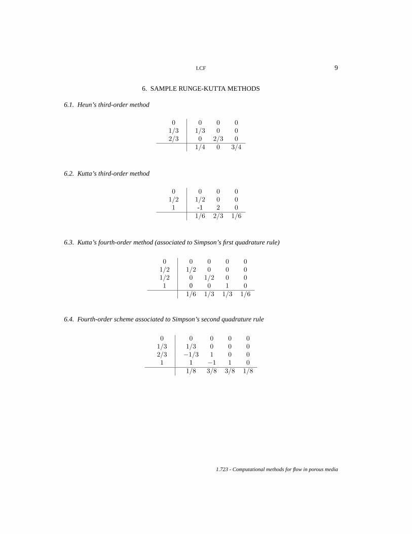
6. SAMPLE RUNGE-KUTTA METHODS

6.1. Heun’s third-order method

0 0 0 01/3 1/3 0 02/3 0 2/3 0

1/4 0 3/4

6.2. Kutta’s third-order method

0 0 0 01/2 1/2 0 01 -1 2 0

1/6 2/3 1/6

6.3. Kutta’s fourth-order method (associated to Simpson’s first quadrature rule)

0 0 0 0 01/2 1/2 0 0 01/2 0 1/2 0 01 0 0 1 0

1/6 1/3 1/3 1/6

6.4. Fourth-order scheme associated to Simpson’s second quadrature rule

0 0 0 0 01/3 1/3 0 0 02/3 −1/3 1 0 01 1 −1 1 0

1/8 3/8 3/8 1/8



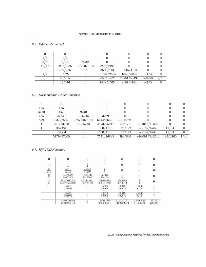
6.5. Fehlberg’s method

0 0 0 0 0 0 01/4 1/4 0 0 0 0 03/8 3/32 9/32 0 0 0 0

12/13 1932/2197 −7200/2197 7296/2197 0 0 01 439/216 −8 3680/513 −845/4104 0 0

1/2 −8/27 2 −3544/2565 1859/4104 −11/40 016/135 0 6656/12825 28561/56430 −9/50 2/5525/216 0 1408/2565 2197/4104 −1/5 0

6.6. Dormand and Prince’s method

0 0 0 0 0 0 0 01/5 1/5 0 0 0 0 0 03/10 3/40 9/40 0 0 0 0 04/5 44/45 −56/15 32/9 0 0 0 08/9 19372/6561 −25360/2187 64448/6561 −212/729 0 0 01 9017/3168 −355/33 46732/5247 49/176 −51013/18656 0 01 35/384 0 500/1113 125/192 −2187/6784 11/84 0

35/384 0 500/1113 125/192 −2187/6784 11/84 05179/57600 0 7571/16695 393/640 −92097/339200 187/2100 1/40

6.7. Bijl’s DIRK method

0 0 0 0 0 0 012

14

14 0 0 0 0

83250

861162500

−174331250

14 0 0 0

3150

501202934652500

−6544412922500

174375388108

14 0 0

720

15267082809155376265600

−71443401120774400

730878875902184768

22853958070912

14 0

1 82889524892 0 15625

8366469875102672

−22608211

14

82889524892 0 15625

8366469875102672

−22608211

14

458657059929645900160 0 178811875

9450685448142202251159782912

−370063711593932

61727225920


LCF 11

7. IMPLEMENTATION OF EXPLICIT RUNGE-KUTTA METHODS

7.1. A first, non-PDE example

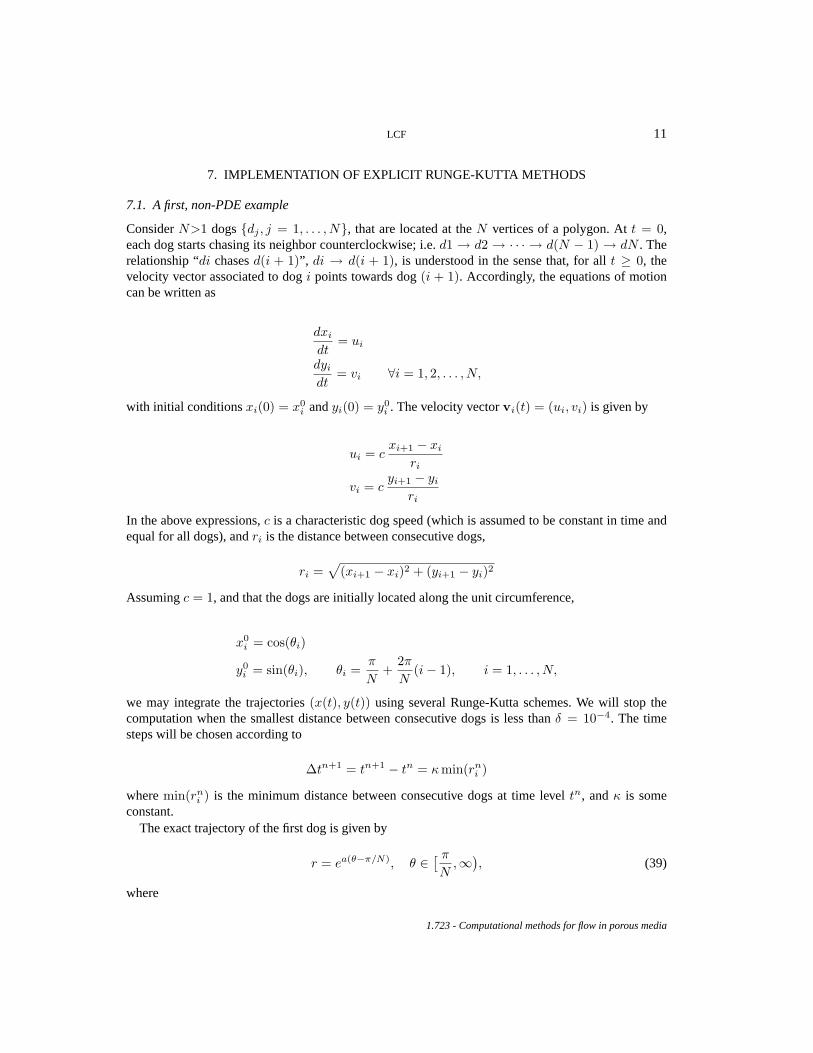
ConsiderN>1 dogs{dj , j = 1, . . . , N}, that are located at theN vertices of a polygon. Att = 0,each dog starts chasing its neighbor counterclockwise; i.e.d1 → d2 → · · · → d(N − 1) → dN . Therelationship “di chasesd(i + 1)”, di → d(i + 1), is understood in the sense that, for allt ≥ 0, thevelocity vector associated to dogi points towards dog(i + 1). Accordingly, the equations of motioncan be written as

dxi

dt= ui

dyi

dt= vi ∀i = 1, 2, . . . , N,

with initial conditionsxi(0) = x0i andyi(0) = y0

i . The velocity vectorvi(t) = (ui, vi) is given by

ui = cxi+1 − xi

ri

vi = cyi+1 − yi

ri

In the above expressions,c is a characteristic dog speed (which is assumed to be constant in time andequal for all dogs), andri is the distance between consecutive dogs,

ri =√

(xi+1 − xi)2 + (yi+1 − yi)2

Assumingc = 1, and that the dogs are initially located along the unit circumference,

x0i = cos(θi)

y0i = sin(θi), θi =

π

N+

2π

N(i− 1), i = 1, . . . , N,

we may integrate the trajectories(x(t), y(t)) using several Runge-Kutta schemes. We will stop thecomputation when the smallest distance between consecutive dogs is less thanδ = 10−4. The timesteps will be chosen according to

∆tn+1 = tn+1 − tn = κ min(rni )

wheremin(rni ) is the minimum distance between consecutive dogs at time leveltn, andκ is some

constant.The exact trajectory of the first dog is given by

r = ea(θ−π/N), θ ∈ [ π

N,∞)

, (39)

where



a =cos

2π

N− 1

sin2πN

. (40)

The trajectories of the other dogs are identical, but shifted2π

N.

This problem is solved by the codedogsrk.m , which can be found in the folderexample_RK . Eachstep of ans-stage explicit RK method works as follows:

- For every stage, we need to compute the stage value using thef ’s evaluated at previous stages,as.


s∑

j=1


Once we compute the stage value,uuuuuuuuuuuuuui, we storef(t + ci∆t, uuuuuuuuuuuuuui). In the code, this corresponds to

for istage=1:nstage;accum= u0;for jstage= 1:istage-1;

accum= accum + dt*ARK(istage,jstage)*F(:,jstage);end;

[f,r]= odefun(t+cRK(istage)*dt,accum);F(:,istage)= f;

end;

- Once all the stage values and their associatef ’s have been computed, we advance the solution as


s∑

i=1

bikkkkkkkkkkkkkki, kkkkkkkkkkkkkki = ffffffffffffff (tn + ci∆t, uuuuuuuuuuuuuui) . (42)

In the code, this reads

u= u0;for istage= 1:nstage;

u= u + dt*bRK(istage)*F(:,istage);end;

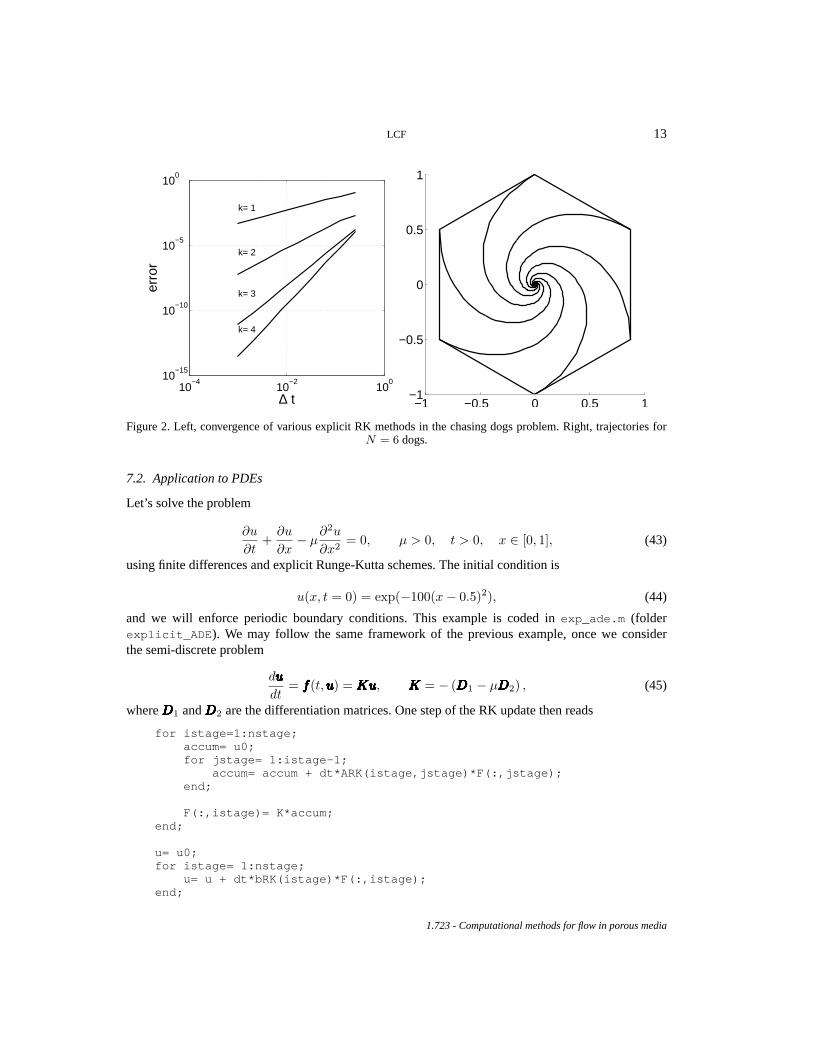
The code may work with RK methods of orders 1 to 4 (their Butcher’s tableaux are given inButcherT.m . Convergence results and a sample simulation withN = 6 dogs are shown in Figure 2.The convergence study was carried out using the codedogsrk_conv.m .


LCF 13

10−4

10−2

100

10−15

10−10

10−5

100

∆ t

erro

r

k= 1

k= 2

k= 3

k= 4

−1 −0.5 0 0.5 1−1

−0.5

0

0.5

1

Figure 2. Left, convergence of various explicit RK methods in the chasing dogs problem. Right, trajectories forN = 6 dogs.

7.2. Application to PDEs

Let’s solve the problem

∂u

∂t+

∂u

∂x− µ

∂2u

∂x2= 0, µ > 0, t > 0, x ∈ [0, 1], (43)

using finite differences and explicit Runge-Kutta schemes. The initial condition is

u(x, t = 0) = exp(−100(x− 0.5)2), (44)

and we will enforce periodic boundary conditions. This example is coded inexp_ade.m (folderexplicit_ADE ). We may follow the same framework of the previous example, once we considerthe semi-discrete problem

duuuuuuuuuuuuuu

dt= ffffffffffffff(t, uuuuuuuuuuuuuu) = KKKKKKKKKKKKKKuuuuuuuuuuuuuu, KKKKKKKKKKKKKK = − (DDDDDDDDDDDDDD1 − µDDDDDDDDDDDDDD2) , (45)

whereDDDDDDDDDDDDDD1 andDDDDDDDDDDDDDD2 are the differentiation matrices. One step of the RK update then reads

for istage=1:nstage;accum= u0;for jstage= 1:istage-1;


F(:,istage)= K*accum;end;





8. IMPLEMENTATION OF IMPLICIT RUNGE-KUTTA METHODS

8.1. Linear case

In the case of (diagonally) implicit RK methods, since the evaluation of the stage valuesuuuuuuuuuuuuuui involvesffffffffffffff i itself, we need to solve a system of equations. Let us start with the same linear advection-diffusionequation of the previous example,

∂u

∂t+

∂u

∂x− µ

∂2u

∂x2= 0, µ > 0, t > 0, x ∈ [0, 1], (46)

initial condition

u(x, t = 0) = exp(−100(x− 0.5)2), (47)

and periodic boundary conditions.Remember that the general form of the RK update is given by


s∑

i=1

bikkkkkkkkkkkkkki, kkkkkkkkkkkkkki = ffffffffffffff (tn + ci∆t, uuuuuuuuuuuuuui) , (48)

with stage values


s∑

j=1


In the present case, since we consider DIRK schemes only, the stage values will be given by


i∑

j=1

aijkkkkkkkkkkkkkkj , (50)

with

kkkkkkkkkkkkkkj = KKKKKKKKKKKKKKuuuuuuuuuuuuuuj , KKKKKKKKKKKKKK = − (DDDDDDDDDDDDDD1 − µDDDDDDDDDDDDDD2) , (51)

whereDDDDDDDDDDDDDD1 andDDDDDDDDDDDDDD2 are the differentiation matrices. Thus, the computation of stage values may be writtenas


i−1∑

j=1

aijkkkkkkkkkkkkkkj + ∆taiiKKKKKKKKKKKKKKuuuuuuuuuuuuuui. (52)

Rearranging the above expression, we arrive at a system of linear equations of the form

(IIIIIIIIIIIIII −∆taiiKKKKKKKKKKKKKK)uuuuuuuuuuuuuui = uuuuuuuuuuuuuun + ∆t

i−1∑

j=1

aijkkkkkkkkkkkkkkj , (53)

that needs to be solved in order to getuuuuuuuuuuuuuui.The codeimp_ade.m (folder implicit_ADE ) solves this problem using backward Euler and Bijl’s

DIRK method. One step of a DIRK scheme is coded as


LCF 15

u0= u;for istage=1:nstage;

accum= u0;for jstage= 1:istage-1;


%Solve system of equationsImpmat= eye(N)-dt*ARK(istage,istage)*K;u= Impmat\accum;%Compute f(u_i)F(:,istage)= K*u;

end;

%Final updateu= u0;for istage= 1:nstage;


Note that, in the present case, the matrixKKKKKKKKKKKKKK could have been precomputed and inverted only once atthe beginning.



8.2. Nonlinear case: fully implicit vs. implicit-explicit

Our model problem for the nonlinear case is the Kuramoto-Sivashinsky equation

∂u

∂t+

∂

∂x

(12u2

)+

∂2u

∂x2+

∂4u

∂x4= 0 (54)

This equation is solved in[0, 32π] with periodic boundary conditions. The initial condition is given by

u(x, t = 0) = cos(x/16) (1 + sin(x/16) (55)

In this equation, the low-order (advective) term is nonlinear, whereas the higher-order terms are linear.The fact that a fourth-order term is present makes the equation very stiff. There are two main strategiesthat could be followed: fully implicit time stepping, where the three terms are advanced implicitly, andimplicit-explicit, where the advective term is advanced explicitly and the higher-order terms implicitly.The latter strategy has the advantage that we solve linear systems of equations. In the former, we needto use Newton iterations to solve the resulting nonlinear systems.

The fully nonlinear strategy is implemented in the codeimp_ks.m (folder implicit_KS ). One stepof a DIRK scheme is implemented as




%Solve system of nonlinear equationsr= 1;while(r>10ˆ-6);

%JacobianJac= eye(N) + dt*ARK(istage,istage)*(D1*diag(u) + D2 + D4);%ResidualR= u - accum + dt*ARK(istage,istage)*(D1*(0.5*u.*u) + D2*u + D4*u);%Updatedeltau= -Jac\R;u= u+deltau;r= norm(deltau);

end;

F(:,istage)= -(D1*(0.5*u.*u) + D2*u + D4*u);end;



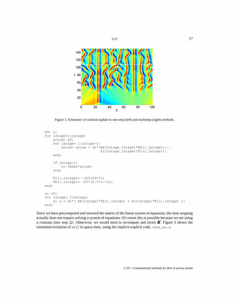
The implicit-explicit strategy is implemented in the codeimex_ks.m (folder imex_KS ). We use oneof the theARK2 methods developed in [6].The advantage of an IMEX formulation is that the systemsthat we need to solve are linear, and therefore we do not need several Newton iterations as in the fullyimplicit scheme. One step of the IMEX-RK scheme reads


LCF 17

Figure 3. Schematic of solution update in one-step (left) and multistep (right) methods.



accum= accum + dt*(AE(istage,jstage)*KE(:,jstage)+...AI(istage,jstage)*KI(:,jstage));

end;

if istage>1;u= IKmat*accum;

end;

KI(:,istage)= -(D2+D4)*u;KE(:,istage)= -D1*(0.5*u.*u);

end;


u= u + dt*( bE(istage)*KE(:,istage) + bI(istage)*KI(:,istage) );end;

Since we have precomputed and inverted the matrix of the linear system of equations, the time steppingactually does not require solving a system of equations. Of course this is possible because we are usinga constant time step∆t. Otherwise, we would need to recompute and invertKKKKKKKKKKKKKK. Figure 3 shows thesimulated evolution ofu(x) in space-time, using the implicit-explicit code,imex_ks.m



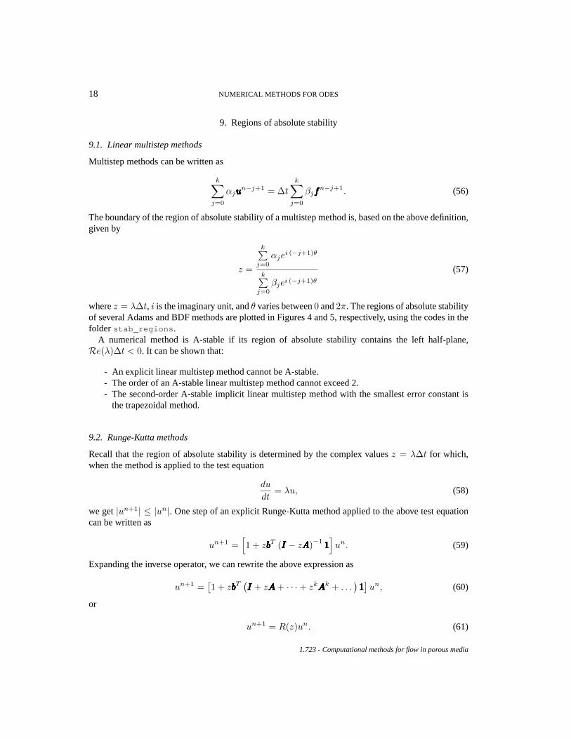
9. Regions of absolute stability

9.1. Linear multistep methods

Multistep methods can be written as

k∑

j=0

αjuuuuuuuuuuuuuun−j+1 = ∆t

k∑

j=0

βjffffffffffffffn−j+1. (56)

The boundary of the region of absolute stability of a multistep method is, based on the above definition,given by

z =

k∑j=0

αjei (−j+1)θ

k∑j=0

βjei (−j+1)θ

(57)

wherez = λ∆t, i is the imaginary unit, andθ varies between0 and2π. The regions of absolute stabilityof several Adams and BDF methods are plotted in Figures 4 and 5, respectively, using the codes in thefolder stab_regions .

A numerical method is A-stable if its region of absolute stability contains the left half-plane,Re(λ)∆t < 0. It can be shown that:

- An explicit linear multistep method cannot be A-stable.- The order of an A-stable linear multistep method cannot exceed 2.- The second-order A-stable implicit linear multistep method with the smallest error constant is

the trapezoidal method.

9.2. Runge-Kutta methods

Recall that the region of absolute stability is determined by the complex valuesz = λ∆t for which,when the method is applied to the test equation

du

dt= λu, (58)

we get|un+1| ≤ |un|. One step of an explicit Runge-Kutta method applied to the above test equationcan be written as

un+1 =[1 + zbbbbbbbbbbbbbbT (IIIIIIIIIIIIII − zAAAAAAAAAAAAAA)−1 11111111111111

]un. (59)

Expanding the inverse operator, we can rewrite the above expression as

un+1 =[1 + zbbbbbbbbbbbbbbT

(IIIIIIIIIIIIII + zAAAAAAAAAAAAAA + · · ·+ zkAAAAAAAAAAAAAAk + . . .

)11111111111111]un, (60)

or

un+1 = R(z)un. (61)


LCF 19

Figure 4. Regions of absolute stability of Adams methods. Left, Adams-Bashforth. Right, Adams-Moulton.

Figure 5. Regions of absolute stability of backward differentiation formulas. Left,k = 1− 4. Right,k = 4− 6.



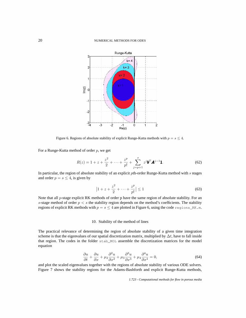
Figure 6. Regions of absolute stability of explicit Runge-Kutta methods withp = s ≤ 4.

For a Runge-Kutta method of orderp, we get

R(z) = 1 + z +z2

2+ · · ·+ zp

p!+

s∑

j=p+1

zjbbbbbbbbbbbbbbTAAAAAAAAAAAAAAj−111111111111111. (62)

In particular, the region of absolute stability of an explicitpth-order Runge-Kutta method withs stagesand orderp = s ≤ 4, is given by

∣∣1 + z +z2

2+ · · ·+ zp

p!

∣∣ ≤ 1 (63)

Note that allp-stage explicit RK methods of order p have the same region of absolute stability. For ans-stage method of orderp < s the stability region depends on the method’s coefficients. The stabilityregions of explicit RK methods withp = s ≤ 4 are plotted in Figure 6, using the coderegions_RK.m .

10. Stability of the method of lines

The practical relevance of determining the region of absolute stability of a given time integrationscheme is that the eigenvalues of our spatial discretization matrix, multiplied by∆t, have to fall insidethat region. The codes in the folderstab_MOL assemble the discretization matrices for the modelequation

∂u

∂t+

∂u

∂x+ µ2

∂2u

∂x2+ µ3

∂3u

∂x3+ µ4

∂4u

∂x4= 0, (64)

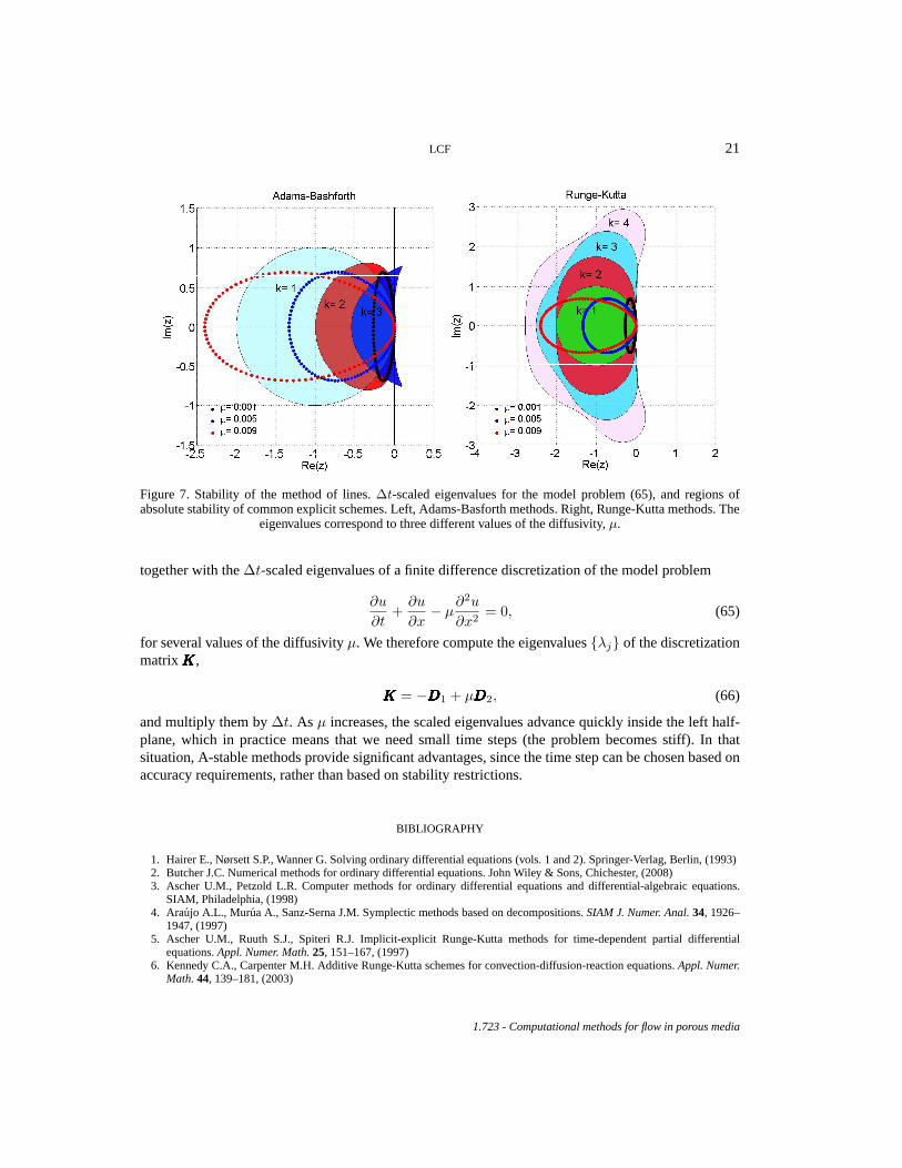
and plot the scaled eigenvalues together with the regions of absolute stability of various ODE solvers.Figure 7 shows the stability regions for the Adams-Bashforth and explicit Runge-Kutta methods,


LCF 21

Figure 7. Stability of the method of lines.∆t-scaled eigenvalues for the model problem (65), and regions ofabsolute stability of common explicit schemes. Left, Adams-Basforth methods. Right, Runge-Kutta methods. The

eigenvalues correspond to three different values of the diffusivity,µ.

together with the∆t-scaled eigenvalues of a finite difference discretization of the model problem

∂u

∂t+

∂u

∂x− µ

∂2u

∂x2= 0, (65)

for several values of the diffusivityµ. We therefore compute the eigenvalues{λj} of the discretizationmatrixKKKKKKKKKKKKKK,

KKKKKKKKKKKKKK = −DDDDDDDDDDDDDD1 + µDDDDDDDDDDDDDD2, (66)

and multiply them by∆t. As µ increases, the scaled eigenvalues advance quickly inside the left half-plane, which in practice means that we need small time steps (the problem becomes stiff). In thatsituation, A-stable methods provide significant advantages, since the time step can be chosen based onaccuracy requirements, rather than based on stability restrictions.

BIBLIOGRAPHY

1. Hairer E., Nørsett S.P., Wanner G. Solving ordinary differential equations (vols. 1 and 2). Springer-Verlag, Berlin, (1993)2. Butcher J.C. Numerical methods for ordinary differential equations. John Wiley & Sons, Chichester, (2008)3. Ascher U.M., Petzold L.R. Computer methods for ordinary differential equations and differential-algebraic equations.

SIAM, Philadelphia, (1998)4. Araujo A.L., Murua A., Sanz-Serna J.M. Symplectic methods based on decompositions.SIAM J. Numer. Anal.34, 1926–

1947, (1997)5. Ascher U.M., Ruuth S.J., Spiteri R.J. Implicit-explicit Runge-Kutta methods for time-dependent partial differential

equations.Appl. Numer. Math.25, 151–167, (1997)6. Kennedy C.A., Carpenter M.H. Additive Runge-Kutta schemes for convection-diffusion-reaction equations.Appl. Numer.

Math.44, 139–181, (2003)


numerical methods for first order odes

Documents