numerical linear algebra: iterative methodspingali/cse392/2011sp/lectures/iterative.pdf ·...

Numerical Linear Algebra: iterative methods

Victor Eijkhout

Two different approachesSolve Ax = b

Direct methods:

• Deterministic

• Exact up to machine precision

• Expensive (in time and space)

Iterative methods:

• Only approximate

• Cheaper in space and (possibly) time

• Convergence not guaranteed

Pingali scicomp 2011 — 2

Iterative methods

Choose any x0 and repeat

xk+1 = Bxk + c

until ‖xk+1 − xk‖2 < ε or until ‖xk+1−xk‖2‖xk‖ < ε


Example of iterative solutionExample system 10 0 1

1/2 7 11 0 6

x1x2x3

=

2198

with solution (2, 1, 1).

Suppose you know (physics) that solution components are roughlythe same size, and observe the dominant size of the diagonal, then10

76

x1x2x3

=

2198

might be a good approximation: solution (2.1, 9/7, 8/6).


Iterative example′Example system 10 0 1

1/2 7 11 0 6

x1x2x3

=

2198

with solution (2, 1, 1).

Also easy to solve: 101/2 7

1 0 6

x1x2x3

=

2198

with solution (2.1, 7.95/7, 5.9/6).


Iterative example′′

Instead of solving Ax = b we solved Lx = b. Look for the missingpart: x = x + ∆x , then A∆x = Ax − b ≡ r . Solve again L∆x = r

and update ˜x = x − ∆x .

iteration 1 2 3x1 2.1000 2.0017 2.000028x2 1.1357 1.0023 1.000038x3 0.9833 0.9997 0.999995

Two decimals per iteration. This is not typical

Exact system solving: O(n3) cost; iteration: O(n2) per iteration.Potentially cheaper if the number of iterations is low.


Abstract presentation

• To solve Ax = b; too expensive; suppose K ≈ A and solvingKx = b is possible

• Define Kx0 = b, then error correction e0 = x − x0, andA(x0 + e0) = b

• so Ae0 = b − Ax0 = r0; this is again unsolvable, so

• K e0 and x1 = x0 + e0.

• now iterate: e1 = x − x1, Ae1 = b − Ax1 = r1 et cetera


Error analysis

• One step

r1 = b − Ax1 = b − A(x0 + e0) (1)

= r0 − AK−1r0 (2)

= (I − AK−1)r0 (3)

• Inductively: rn = (I −AK−1)nr0 so rn ↓ 0 if |λ(I −AK−1)| < 1Geometric reduction (or amplification!)

• This is ‘stationary iteration’: every iteration step the same.Simple analysis, limited applicability.


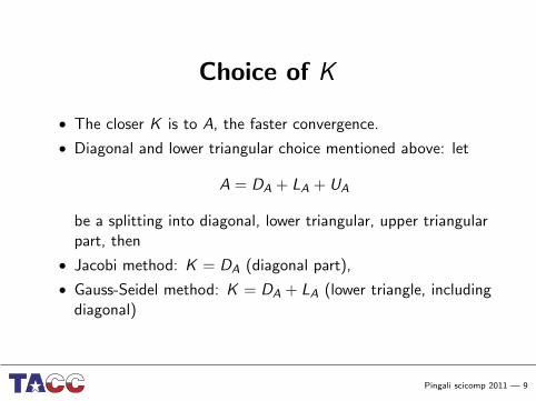
Choice of K

• The closer K is to A, the faster convergence.

• Diagonal and lower triangular choice mentioned above: let

A = DA + LA + UA

be a splitting into diagonal, lower triangular, upper triangularpart, then

• Jacobi method: K = DA (diagonal part),

• Gauss-Seidel method: K = DA + LA (lower triangle, includingdiagonal)


Computationally

IfA = K − N

thenAx = b ⇒ Kx = Nx + b ⇒ Kxi+1 = Nxi + b

Equivalent to the above, and you don’t actually need to form theresidual.


Jacobi

K = DA

Algorithm:

for k = 1, . . . until convergence, do:for i = 1 . . . n:

x(k+1)i = a−1ii (

∑j 6=i aijx

(k)j + bi )

Implementation:


ti = a−1ii (−∑

j 6=i aijxj + bi )

copy x ← t


Jacobi in pictures:


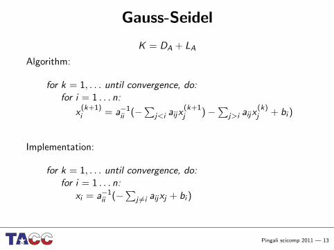
Gauss-Seidel

K = DA + LA

Algorithm:


x(k+1)i = a−1ii (−

∑j<i aijx

(k+1j )−

∑j>i aijx

(k)j + bi )

Implementation:


xi = a−1ii (−∑

j 6=i aijxj + bi )


GS in pictures:


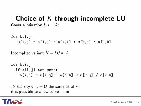
Choice of K through incomplete LUGauss elimination LU = A:

for k,i,j:

a[i,j] = a[i,j] - a[i,k] * a[k,j] / a[k,k]

Incomplete variant K = LU ≈ A:

for k,i,j:

if a[i,j] not zero:

a[i,j] = a[i,j] - a[i,k] * a[k,j] / a[k,k]

⇒ sparsity of L + U the same as of Ait is possible to allow some fill-in


Stopping tests

When to stop converging? Can size of the error be guaranteed?

• Direct tests on error en = x − xn impossible; two choices

• Relative change in the computed solution small:

‖xn+1 − xn‖/‖xn‖ < ε

• Residual small enough:

‖rn‖ = ‖Axn − b‖ < ε

Without proof: both imply that the error is less than some other ε′.


General form of iterative methods 1.System Ax = b has the same solution as K−1Ax = K−1b.

Let x be a guess and

r = K−1Ax − K−1b.

thenx = A−1b = x − A−1K r = x − (K−1A)−1r .

Using Cayley-Hamilton theorem:

x = x − π(K−1A)K−1r = x − K−1π(AK−1)r .

Iterative scheme:

xi+1 = x0 + K−1π(i)(AK−1)r0 (4)


Convergence theory for residuals

xi+1 = x0 + K−1π(i)(AK−1)r0

Multiply by A and subtract b:

ri+1 = r0 + π(i)(AK−1)r0

So:ri = π(i)(AK−1)r0

where π(i) is a polynomial of degree i with π(i)(0) = 1.

What polynomial sequence minimizes the residual?


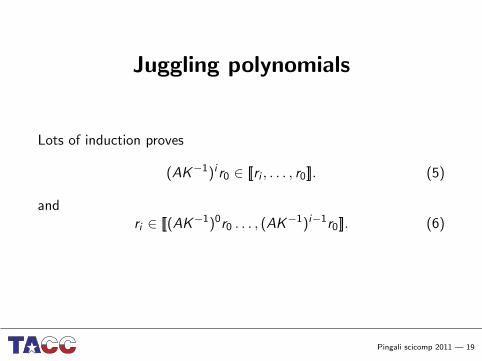
Juggling polynomials

Lots of induction proves

(AK−1)i r0 ∈ [[ri , . . . , r0]]. (5)

andri ∈ [[(AK−1)0r0 . . . , (AK−1)i−1r0]]. (6)


General form of iterative methods 3.

xi+1 = x0 +∑j≤i

K−1rjαji .

or equivalently:

xi+1 = xi +∑j≤i

K−1rjαji .


More residual identities

xi+1 = xi +∑j≤i

K−1rjαji .

gives

ri+1 = ri +∑j≤i

AK−1rjαji .

More throwing of formulas:

ri+1γi+1,i = AK−1ri +∑j≤i

rjγji

where γi+1,i =∑

j≤i γji .



ri+1γi+1,i = AK−1ri +∑j≤i

rjγji

and γi+1,i =∑

j≤i γji .

Write this as AK−1R = RH where

H =

−γ11 −γ12 . . .γ21 −γ22 −γ23 . . .0 γ32 −γ33 −γ34∅ . . .

. . .. . .

. . .

H is a Hessenberg matrix, and note zero column sums.

Divide A out:xi+1γi+1,i = K−1ri +

∑j≤i

xjγji



ri = Axi − b

xi+1γi+1,i = K−1ri +∑

j≤i xjγji

ri+1γi+1,i = AK−1ri +∑

j≤i rjγji

where γi+1,i =∑

j≤i γji .


OrthogonalityIdea one:

If you can make all your residuals orthogonal to eachother, and the matrix is of dimension n, then after niterations you have to have converged: it is not possibleto have an n + 1-st residuals that is orthogonal andnonzero.

Idea two:

The sequence of residuals spans a series of subspaces ofincreasing dimension; by orthogonalizing the error is thedistance between r0 and these spaces. This means thatthe error will be decreasing.


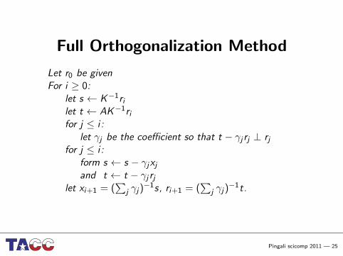
Full Orthogonalization Method

Let r0 be givenFor i ≥ 0:

let s ← K−1rilet t ← AK−1rifor j ≤ i :

let γj be the coefficient so that t − γj rj ⊥ rjfor j ≤ i :

form s ← s − γjxjand t ← t − γj rj

let xi+1 = (∑

j γj)−1s, ri+1 = (

∑j γj)

−1t.


Modified Gramm-Schmidt

Let r0 be givenFor i ≥ 0:

let s ← K−1rilet t ← AK−1rifor j ≤ i :

let γj be the coefficient so that t − γj rj ⊥ rjform s ← s − γjxjand t ← t − γj rj

let xi+1 = (∑

j γj)−1s, ri+1 = (

∑j γj)

−1t.


Coupled recurrences form

xi+1 = xi −∑j≤i

αjiK−1rj (7)

This equation is often split as

• Update iterate with search direction: direction:

xi+1 = xi − δipi ,

• Construct search direction from residuals:

pi = K−1ri +∑j<i

βijK−1rj .

Inductively:

pi = K−1ri +∑j<i

γijpj ,


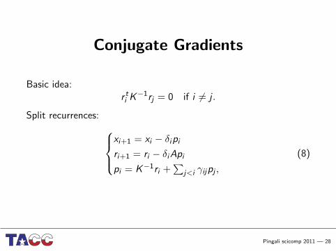
Conjugate Gradients

Basic idea:r ti K−1rj = 0 if i 6= j .

Split recurrences: xi+1 = xi − δipi

ri+1 = ri − δiApi

pi = K−1ri +∑

j<i γijpj ,

(8)


Derivation 1.

Let

• x1, r1, p1 are the current iterate, residual, and search direction.Note that the subscript 1 does not denote the iterationnumber here.

• x2, r2, p2 are the iterate, residual, and search direction that weare about to compute. Again, the subscript does not equalthe iteration number.

• X0,R0,P0 are all previous iterates, residuals, and searchdirections bundled together in a block of vectors.


Derivation 2.

In terms of these quantities, the update equations are thenx2 = x1 − δ1p1

r2 = r1 − δiAp1

p2 = K−1r2 + υ12p1 + P0u02

(9)

where δ1, υ12 are scalars, and u02 is a vector with length thenumber of iterations before the current.


Derivation of scalars

We want:r t2K−1r1 = 0, r t2K−1R0 = 0.

Combining these relations gives us, for instance,

r t1K−1r2 = 0r2 = r1 − δiAK−1p1

}⇒ δ1 =

r t1r1r t1AK−1p1

.

Finding υ12, u02 is a little harder.


Preconditioned Conjugate Gradients

Compute r (0) = b − Ax (0) for some initial guess x (0)

for i = 1, 2, . . .solve Mz (i−1) = r (i−1)

ρi−1 = r (i−1)T z (i−1)

if i = 1p(1) = z (0)

elseβi−1 = ρi−1/ρi−2

p(i) = z (i−1) + βi−1p(i−1)

endifq(i) = Ap(i)

αi = ρi−1/p(i)T q(i)

x (i) = x (i−1) + αip(i)

r (i) = r (i−1) − αiq(i)

check convergence; continue if necessaryend


Observations on iterative methods

• Conjugate gradients: constant storage and inner products;works only for symmetric systems

• GMRES (like FOM): growing storage and inner products:restarting and numerical cleverness

• BiCGstab and QMR: relax the orthogonality


CG derived from minimizationSpecial case of SPD:

For which vector x with ‖x‖ = 1 is f (x) = 1/2x tAx − btx minimal?(10)

Taking derivative:f ′(x) = Ax − b.

Updatexi+1 = xi + piδi

optimal value:

δi = argminδ‖f (xi + piδ)‖ =

r ti pi

pt1Api

Other constants follow from orthogonality.


Parallism

• Vector operations, including inner products

• Matrix vector product

• Preconditioner (K ) application


Parallelism in preconditioners: the problemMvp:

for i=1..n

y[i] = sum over j=1..n a[i,j]*x[j]

In parallel:

for i=myfirstrow..mylastrow

y[i] = sum over j=1..n a[i,j]*x[j]

Preconditioner ILU:

for i=1..n

x[i] = (y[i] - sum over j=1..i-1 ell[i,j]*x[j]) / a[i,i]

parallel:


x[i] = (y[i] - sum over j=1..i-1 ell[i,j]*x[j]) / a[i,i]

Not the same! Pingali scicomp 2011 — 36

Block Jacobi


x[i] = (y[i] - sum over j=myfirstrow..i-1 ell[i,j]*x[j])

/ a[i,i]


Multicolouring

a11 a12a33 a32 a34

a55. . .

. . .. . .

a21 a23 a22a43 a45 a44

. . .. . .

. . .

x1x3x5...

x2x4...

=

y1y3y5...

y2y4...


Parallelism through multicolouring


numerical linear algebra: iterative methodspingali/cse392/2011sp/lectures/iterative.pdf ·...

Documents