numerical computation of the module of a quadrilateral
TRANSCRIPT
University of Helsinki
Master’s thesis
Numerical computation of themodule of a quadrilateral
Author:
Juhana Yrjölä
Supervisors:
Prof. Matti Vuorinen
Ph. D. Antti Rasila
Department of Mathematics and StatisticsPL 68 (Gustaf Hällströmin katu 2b)
00014 University of Helsinki
March 12, 2007

Preface
Writing this thesis has been a long and hard struggle. Considering all the difficultiesI had with this project I have tried to write a simple introduction to the moduleof a quadrilateral, even if nobody ever reads this. I could have put more effort toimprove the readability of the text but unfortunately all projects must come to anend and this project was no exception. This project ended because it needed to endnot because it reached its natural conclusion.
This project would have never been completed without God’s help in the dark-est hours of this work. Therefore I want to give Him all the credit, and my eternalgratitude for completing this work
Furthermore, I thank my supervisors prof. Matti Vuorinen and Ph. D. Antti Rasilafor introducing me to this subject and for their suggestions and corrections to thework itself. Also I thank Mr. Kai Mäkelä for helping me with the English spelling.
Finally, I would like to thank my parents for financial support during this longendeavor.
March 12, 2007Juhana Yrjölä
Contents
Preface 2
1. Introduction 5
2. Preliminaries 52.1. Complex numbers .......................................................................................... 5
2.2. Curves, Jordan domains and quadrilaterals ............................................. 7
2.3. Conformal maps and Riemann mapping theorem................................... 10
2.4. Darboux integral ............................................................................................ 14
2.5. Elliptic integrals ............................................................................................. 16
2.6. Numerical methods and accuracy............................................................... 17
3. The module of a quadrilateral 183.1. The module of a curve family ..................................................................... 18
3.2. The Dirichlet-Neumann problem and the module of a quadrilateral.. 25
4. The Schwarz-Christoffel Mapping 274.1. Numerical implementation of the Schwarz-Christoffel mapping .......... 30
4.2. The module of a quadrilateral and the Schwarz-Christoffel mapping 33
4.3. The Schwarz-Christoffel toolbox................................................................. 35
5. Symmetry properties of the module 395.1. Symmetric quadrilaterals ............................................................................. 41
5.2. Reflection properties of the module of a quadrilateral........................... 47
5.3. Ring domains and the module of a quadrilateral.................................... 52
6. Computational results 546.1. Additive quadrilaterals ................................................................................. 54
6.2. The module of a quadrilateral under movement of one vertex ............ 59
7. Other numerical methods 687.1. Challis & Burley iteration............................................................................ 68
7.2. Heikkala-Vamanamurthy-Vuorinen iteration............................................ 71
7.3. Numerical methods for solving partial differential equations ............... 72
4 JUHANA YRJÖLÄ
List of special symbols and abbreviations 73
Appendix A. Numerical evaluation of the elliptic in-tegrals of the first kind 74
Appendix B. Matlab programs and scripts 76B.1. Matlab program: Challis & Burley iteration with relaxation.............. 76
B.2. Matlab program: Challis & Burley iteration with relaxation and cs. 78
B.3. Matlab program: Moving vertex data calculation ................................. 80
B.4. Matlab script: Data ploting........................................................................ 81
Appendix C. Other fields of interest 83C.1. General concepts and symmetry................................................................ 83
C.2. Numerical methods and Harmonic measure............................................ 84
References 85
Index 87
NUMERICAL COMPUTATION OF THE MODULE OF A QUADRILATERAL 5
1. Introduction
The module of a quadrilateral was introduced by H. Grötzsch in the late 1920’s. Itsoon found many applications and become one of the most useful conformal invari-ants. A far reaching generalization, the module of a curve family was introduced bya Finn Lars Ahlfors and his Swedish colleague Arne Beurling in 1950.
The module of a quadrilateral is a positive real number which divides quadrilat-erals into conformal equivalence classes.
2. Preliminaries
The main goal of this section is to provide enough background material to fully un-derstand the rest of this thesis. Results presented in this chapter are quite commonand basic, so the reader who is well versed in mathematics can jump directly tothe next chapter and return here if needed. The list of used symbols with someinformation is available in the appendix.
2.1. Complex numbers.
Complex numbers are a result of gradual development of our number system. Thisdevelopment began with the positive integers, which were used in counting. Muchlater it was noticed that the number system would benefit by having negative inte-gers and zero. Gradual development lead to augmentation of rational and irrationalnumbers and so the real number system R was born. [Spi99, p. 1]
Complex numbers were first introduced as a way to find all roots of the polyno-mial equations by allowing negative square roots. Later other applications werediscovered in many fields like electrostatics and conformal mapping. We assumehere that the reader is familiar with the basic properties and operations of complexnumbers, if this is not the case, good introductory texts are [Spi99] and [Fla83],especially the first one. We use the following notation
z = x + yi x, y ∈ R(2.1)
f(z) = u(x, y) + iv(x, y) x, y ∈ R(2.2)
for a complex variable z and for a complex function f(z), i is the imaginary uniti =
√−1. The functions u(x, y) and v(x, y) are called conjugate functions and they
are real valued.
Since complex numbers are an extended version of real numbers, many results forthe real variables can be extended for complex numbers. Historically one of themost important concepts of the real analysis is the derivative. Derivative gave abirth to a completely new field of mathematics called the calculus1. The definition
1Historically there was a big controversy between Isaac Newton and Gottfried Leibniz aboutwho actually invented the derivative. The quarrel started from the fact that in 1676 Leibniz wasshown at least one unpublished manuscript by Newton while he visited London. It is unknown
6 JUHANA YRJÖLÄ
of the derivative can be extended to complex plane quite easily, since the complexplane is in many ways similar to a Cartesian plane. The definition of the complexderivative is almost identical to the one for real functions.
2.3. Definition (Derivative for complex functions). [Spi99, p. 63]
(2.4) f ′(z) = lim∆z→0
f(z + ∆z) − f(z)
∆z
provided that f(z) is single valued and the limit exists independently of the directionand manner in which ∆z → 0.
Furthermore, if the derivative f ′(z) exists at all points z of a region R, then f(z)is said to be analytic in R and f(z) is called an analytic function. There exists anice and easy way to tell if a function f(z) is analytic or not in R. If function isanalytic in R, then it fulfils the Cauchy-Riemann equations and other conditionsbelow. [Spi99, p. 63]
2.5. Theorem (Cauchy-Riemann equations). [Spi99, p. 63]Let f(z) = u(x, y)+ iv(x, y), then a necessary condition for f(z) to be analytic in aregion R is that u and v satisfy the Cauchy-Riemann equations
(2.6)∂u
∂x=
∂v
∂y,
∂u
∂y= −∂v
∂x.
If the partial derivatives are continuous in R, then the Cauchy-Riemann equationsare sufficient conditions for f(z) to be analytic in R.[Spi99, p. 63]. The proof canbe found for example from [Spi99, pp. 72-73].
Now if the conjugate functions u and v of Theorem 2.5 have a continuous secondpartial derivatives in R, then we get very important set of functions called as har-monic functions. Furthermore we say that the function f(x, y) is harmonic if itsatisfies Laplace’s equation below.[Spi99, pp. 63-64]
2.7. Definition (Laplace’s equation). [Spi99, p. 63][ENC89]Let f(x, y) be a complex function in the complex plane and write
(2.8) ∇2f =∂2f
∂2x+
∂2f
∂2y.
Then f is said to be harmonic if and only if f satisfies the following equation
(2.9) ∇2f = 0,
which is known as the Laplace’s equation. Also if f(x, y) = u(x, y) + iv(x, y) isanalytic, then u and v are harmonic.
what was in those manuscripts. Later Leibniz published the derivative first in 1684. Newtonpublished some of his findings in 1693 and some more in 1704, almost a decade later. CurrentlyIsaac Newton and Gottfried Leibniz are both credited for the discovery.
NUMERICAL COMPUTATION OF THE MODULE OF A QUADRILATERAL 7
2.2. Curves, Jordan domains and quadrilaterals.
2.10. Definition (Metric). [AB98, p. 34]A real valued function d : X ×X → R is a metric on non-empty set X if it satisfies,for every a, b, c ∈ X, the following axioms
M1 d(a, b) ≥ 0 and d(a, a) = 0 and if a 6= b then d(a, b) > 0.M2 (Symmetry) d(a, b) = d(b, a)M3 (Triangle inequality) d(a, c) ≤ d(a, b) + d(b, c).
The real number d(a, b) is the distance from a to b. The pair (X, d) is called a metricspace.
The word curve comes from Latin word curvus which means bent. Therefore onecould define a curve as a line which has been continuously bended to differentgeometric shapes. The simplest curves are lines and circles. Other very old curvesare conic sections which were studied by Plato who lived 430-347 B.C.[EB, V7, p.664]
2.11. Definition (Curve). [Väi71, def. 1.1]Curve in R2 is a continuous mapping γ : [a,b]→ R2, where [a,b] is an interval in R
and R2 is the real plane with infinity.Alternatively we can define curve in the complex plane as a continuous mappingγ : [a,b]→ C, where C is the complex plane with infinity.
For the rest of this thesis, we denote arbitrary curves by γ. Also we call set of curvesa curve family and we denote a curve family by Γ. Sometimes a term path is usedinstead of a curve but in this work these two different terms are equal.[Väi71, def.4.3]
2.12. Definition (Length of curve). [Väi71, def. 1.1]Let γ be a curve, γ : [a,b] → R2 and also let a = t0 ≤ t1 ≤ · · · ≤ tk = b be asubdivision of [a, b]. The supremum of the sums
(2.13) l(γ) =k∑
i=1
|γ(ti) − γ(ti−1)|
over all subdivisions is called the length of γ. Alternatively we can define the lengthof a curve as
(2.14) l(γ) =
∫ b
a
|γ ′(t)|dt,
for a curve that is differentiable.[Fla83, pp. 18-19]
We say that the curve is rectifiable if the length of a curve is finite and curve isnon-rectifiable otherwise [Väi71, def. 1.1]. Furthermore we say that a curve is closedif the starting point and the end point of a curve are the same. We also say that
8 JUHANA YRJÖLÄ
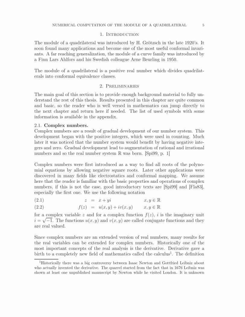
a curve is simple if, and only if, the curve doesn’t cross itself except at the endpoints[Fla83, p. 16]. See Figure 1.
Simple, closed Not simple, closed Simple, not closed Not simple, not closed
Figure 1. Different types of curves.
We say that an arbitrary plane set is a region. We call a region connected if itis pathwise connected, i.e., any two points can be joined by a path that is insidethe region. Furthermore if a region is an open and connected set, then we call it adomain.
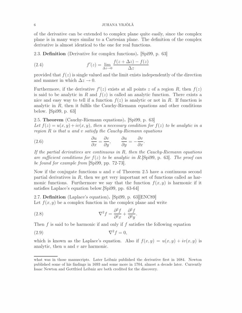
2.15. Definition (Simply and multiply connected domains). [Spi99, p. 93]A connected domain D is called simply connected if any simple closed curve, whichlies in D can be shrunk to a point inside D. A region which is not simply connectedis called multiply connected.
Intuitively, a simply connected domain is a domain, which does not have anyholes or punctures in it. Multiply connected domains have at least one hole orpuncture.[Spi99, p. 94] See Figure 2.
Simply connected domain Not connected region Multiply connected domain
Figure 2. Simply and multiply connected regions.
Simple closed curves have another name in honor for French mathematician CamilleJordan, who studied complex curves.
2.16. Definition (Jordan curve). [Fla83, p. 23]A Jordan curve is a simple closed curve.Alternatively we can say that Jordan curve is a set which is homeomorphic to acircle. [LV73, p. 6].
NUMERICAL COMPUTATION OF THE MODULE OF A QUADRILATERAL 9
Jordan noticed that every Jordan curve divides the plane into an interior domainand an exterior domain and most importantly that this obvious geometric factrequired a proof. However the proof of this Theorem, which is called the Jordancurve Theorem, turned out to be quite difficult.[Fla83, p. 24] Finally in 1905 OswaldVeblen managed to prove it. In 2005 an international team of mathematicians usedcomputer based proof system called Mizar to give a rigorous 200000-line formalproof of the Jordan curve Theorem.
2.17. Definition (Jordan domain). [Fla83, p. 24]A Jordan domain is a bounded domain D, whose boundary is a union of a finitenumber of disjoint Jordan curves, where the orientations of the Jordan curves arechosen such that the interior of D is always lying to the left of the curve.
Note that our definition of a Jordan domain allows holes and punctures.
2.18. Definition (Trilateral). [Hen91, p. 428]A trilateral is simply connected Jordan domain D with three boundary pointsz1, z2, z3 ∈ ∂D. It is assumed that when ∂D is traversed in the positive order(i.e. the domain is on the left side) the points z1, z2, z3, z4 occur in this order. Thepoints are called the vertices of the trilateral.
We denote a trilateral by quadruplet T (D, z1, z2, z3) or just T (z1, z2, z3) or T . Sim-ilarly we define a quadrilateral as
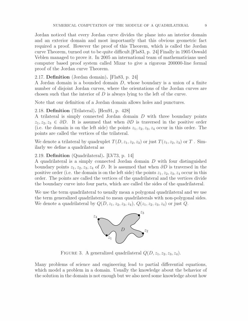
2.19. Definition (Quadrilateral). [LV73, p. 14]A quadrilateral is a simply connected Jordan domain D with four distinguishedboundary points z1, z2, z3, z4 of D. It is assumed that when ∂D is traversed in thepositive order (i.e. the domain is on the left side) the points z1, z2, z3, z4 occur in thisorder. The points are called the vertices of the quadrilateral and the vertices dividethe boundary curve into four parts, which are called the sides of the quadrilateral.
We use the term quadrilateral to usually mean a polygonal quadrilateral and we usethe term generalized quadrilateral to mean quadrilaterals with non-polygonal sides.We denote a quadrilateral by Q(D, z1, z2, z3, z4), Q(z1, z2, z3, z4) or just Q.
D
z4
z3
z2
z1
Figure 3. A generalized quadrilateral Q(D, z1, z2, z3, z4).
Many problems of science and engineering lead to partial differential equations,which model a problem in a domain. Usually the knowledge about the behavior ofthe solution in the domain is not enough but we also need some knowledge about how
10 JUHANA YRJÖLÄ
the solution behaves on the boundary of the domain. Usually the boundary valuesare introduced as extra conditions to be satisfied, and those conditions are calledboundary conditions. The problem usually is to find a function which satistifiescertain conditions inside the domain and some other condition on the boundary.There are two types of boundary conditions that are of great importance namely,the Dirichlet and the Neumann boundary conditions. [Spi99, p. 232]
2.20. Definition (Dirichlet and Neumann boundary conditions). [Spi99, p. 232]Let D be simply connected domain bounded by a simple closed curve γ and let fbe a function, which satisfies Laplace’s equation inside the domain, then
• the Dirichlet boundary condition is a condition that the function f takesprescribed values on the boundary γ.
• the Neumann boundary condition is a condition that the normal derivative∂f
∂ntakes prescribed values on the boundary γ.
Note that it is possible to have different types of boundary conditions on the differentparts of the boundary. Also it is possible that the domain is unbounded, like theupper half plane.
Dirichlet’s problem is a problem where one wants to find a function f , which sat-isfies Laplace’s equation in the domain and also satisfies the Dirichlet boundaryconditions on the boundary. Similarly Neumann’s problem is a problem where onewants to find a function f , which satisfies the Laplace’s equation in the domainand also satisfies the Neumann boundary conditions on the boundary. We can alsotalk about Dirichlet-Neumann problem, where the function f satisfies the Laplace’sequation in the domain and boundary conditions consist of the Dirichlet and theNeumann conditions.[Spi99, p. 232]
Furthermore, it can be shown that solutions to the Dirichlet problem exist andare unique under suitable conditions. For instance if the boundary consists of afinite number of Jordan curves and the boundary values are continuous, then theunique solution is known to exist. Also solutions to the Neumann problem exist andare unique up to an arbitrary small additive constant. In addition, every Neumannproblem can be stated in terms of an appropriately stated Dirichlet problem andthe problem can contain both boundaries.[Spi99, p. 233]
2.3. Conformal maps and Riemann mapping theorem.
Gauss was the first to consider conformal maps as mathematical objects in the1820’s. However the roots of conformal maps are much older and come from theart of map making. The early mapmakers noticed that it is impossible to makedistance preserving map from the spherical object earth, into the plane. Since thedistances could not be preserved, mapmakers tried to preserve directions and suc-ceeded. This lead to maps which preserve angles and the idea of the conformal mapwas born[Por06][Dri02, p. 4].
NUMERICAL COMPUTATION OF THE MODULE OF A QUADRILATERAL 11
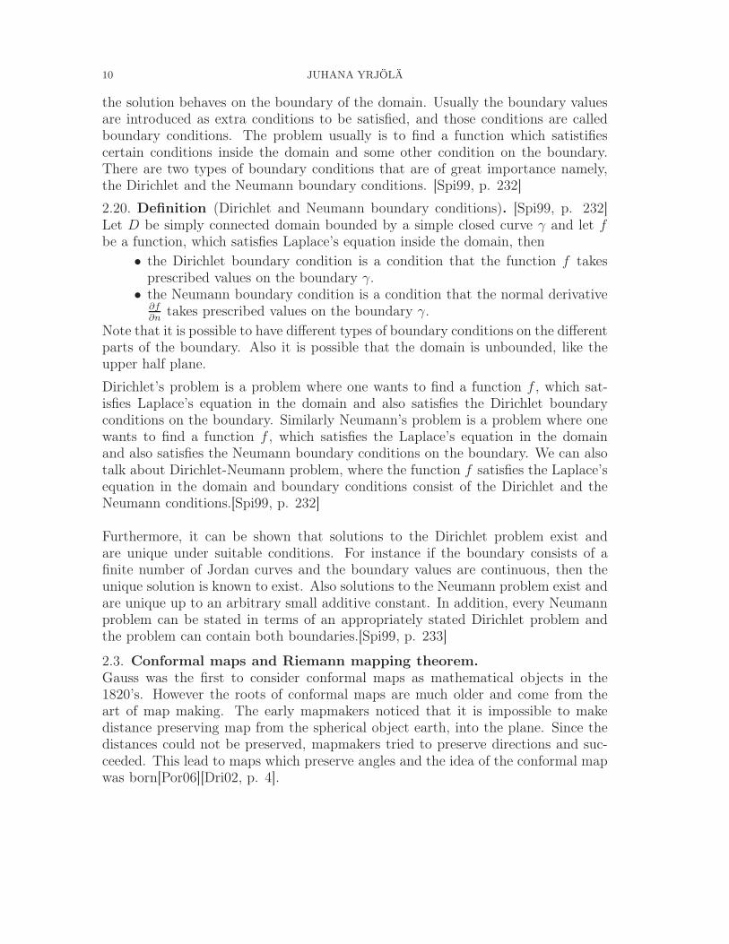
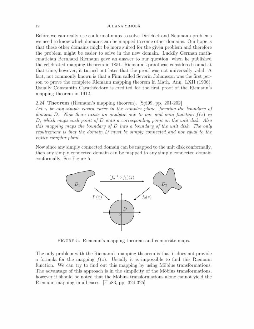
2.21. Definition (Conformal mapping). [Spi99, p. 201]Let f be a mapping from z-plane into w-plane and let γ1 and γ2 be curves in thez-plane, which intersect at point (x0, y0). The curves γ1 and γ2 are mapped intocurves γ′
1 and γ′2 respectively under f . Also the curves γ′
1 and γ′2 intersects at point
(u0, v0). If the mapping f is such that the angle between γ1 and γ2 at (x0, y0) isequal to the angle between γ′
1 and γ′2 at (u0, v0), in both magnitude and sense, then
the mapping f is conformal. See Figure 4.
It should be noted that a conformal map only preserves angles inside the domainand angles on the boundary are not necessarily preserved.
x
y
(x0, y0)
γ1
γ2
α
z plane
u
v (u0, v0)
γ′1
γ′2α
w plane
Figure 4. Mapping f is conformal if it preserves angles in bothmagnitude and sense, inside the domain. The intersection point, andthe end points of the curves γ1 and γ2 are marked with differentsymbols. Note that the curves γ1 and γ2 need not be straight lines.
Now thanks to Gauss and many others we can use conformal maps to solve Dirich-let and Neumann problems. Usually Dirichlet and Neumann problems are quitedifficult to solve. Problem domain might be complex and hard to work with. Oneway to overcome these difficulties is by modifying the domain into something sim-pler by conformal maps and solve the problem in the simplified domain. This ispossible because Dirichlet and Neumann problems are conformal invariants.[Spi99,p. 232][Dri02, p. 4]
2.22. Theorem (Harmonic functions under conformal mapping). [Kre05, p. 754]Let Φ∗ be harmonic in a domain D∗ in the w-plane. Suppose that w = u+ iv = f(z)is analytic in a domain D in the z-plane and maps D conformally onto D∗. Thenthe function
(2.23) Φ(x, y) = Φ∗(u(x, y), v(x, y))
is harmonic in D.
Proof. For the proof see [Kre05, p. 754].
12 JUHANA YRJÖLÄ
Before we can really use conformal maps to solve Dirichlet and Neumann problemswe need to know which domains can be mapped to some other domains. Our hope isthat these other domains might be more suited for the given problem and thereforethe problem might be easier to solve in the new domain. Luckily German math-ematician Bernhard Riemann gave an answer to our question, when he publishedthe celebrated mapping theorem in 1851. Riemann’s proof was considered sound atthat time, however, it turned out later that the proof was not universally valid. Afact, not commonly known is that a Finn called Severin Johansson was the first per-son to prove the complete Riemann mapping theorem in Math. Ann. LXII (1906).Usually Constantin Carathéodory is credited for the first proof of the Riemann’smapping theorem in 1912.
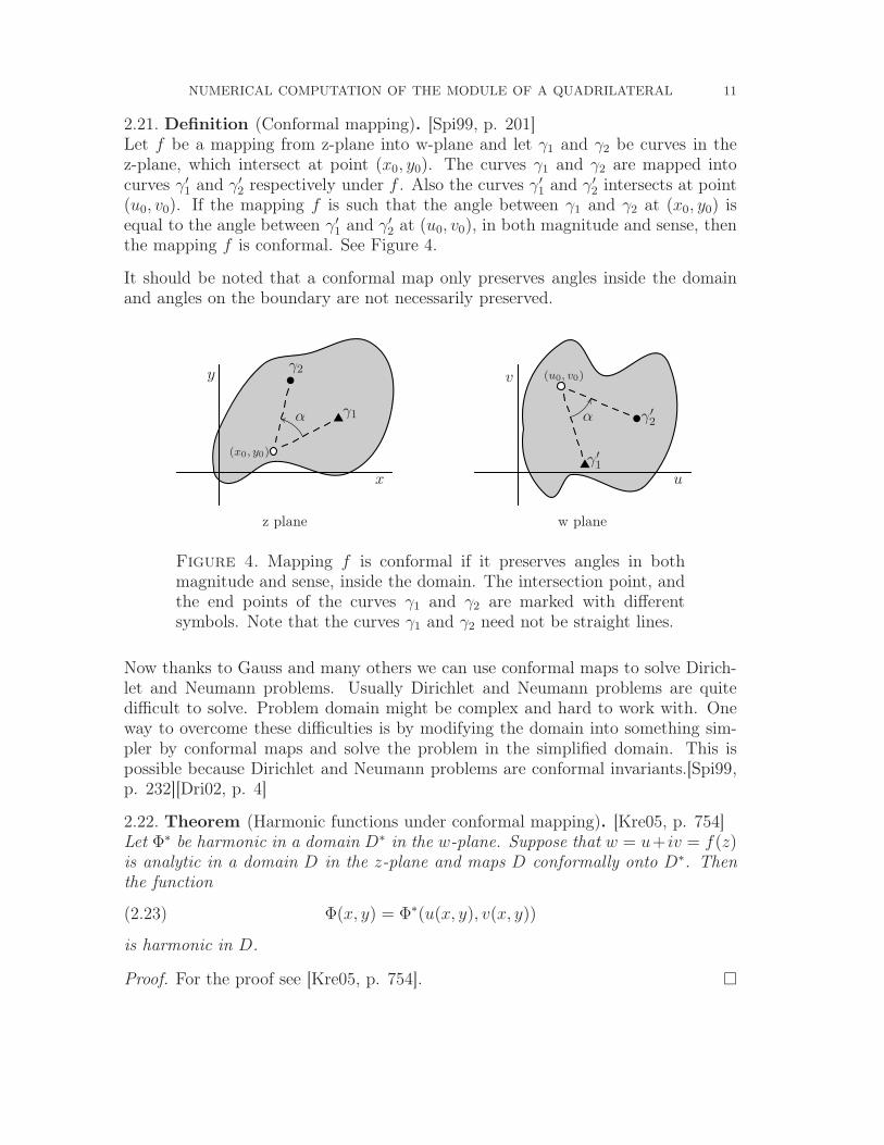
2.24. Theorem (Riemann’s mapping theorem). [Spi99, pp. 201-202]Let γ be any simple closed curve in the complex plane, forming the boundary ofdomain D. Now there exists an analytic one to one and onto function f(z) inD, which maps each point of D onto a corresponding point on the unit disk. Alsothis mapping maps the boundary of D into a boundary of the unit disk. The onlyrequirement is that the domain D must be simply connected and not equal to theentire complex plane.
Now since any simply connected domain can be mapped to the unit disk conformally,then any simply connected domain can be mapped to any simply connected domainconformally. See Figure 5.
0
D
D1 D2
(f−12 f1)(z)
f1(z) f2(z)
Figure 5. Riemann’s mapping theorem and composite maps.
The only problem with the Riemann’s mapping theorem is that it does not providea formula for the mapping f(z). Usually it is impossible to find this Riemannfunction. We can try to find out this mapping by using Möbius transformations.The advantage of this approach is in the simplicity of the Möbius transformations,however it should be noted that the Möbius transformations alone cannot yield theRiemann mapping in all cases. [Fla83, pp. 324-325]
NUMERICAL COMPUTATION OF THE MODULE OF A QUADRILATERAL 13
2.25. Definition (Möbius transformation). [Fla83, p. 304]Let a, b, c, d be given complex parameters, then the Möbius transformation withthe given parameters is
(2.26) w(z) =az + b
cz + dad − bc 6= 0,
where z ∈ C ∪ ∞.Möbius transformation is sometimes called Bilinear or Fractional linear transforma-tion.
Here we just summarize the most important properties of the Möbius transfor-mations. For proofs and other discussion see [Fla83, pp. 306-309] and [Spi99, pp.203, 216-217] or other conformal mapping texts.
• Möbius transformation is a conformal mapping.• Möbius transformation is a combination of the transformations of transla-
tion, rotation, stretching and inversion.• Möbius transformations is one-to-one and onto mapping (hence invertible).• Möbius transformation preserves circles. Circles are mapped to circles under
Möbius transformations, where straight line is circle with a infinite radius.• Möbius transformation maps any three distinct points into any three distinct
points.• Composition of Möbius transformations is a Möbius transformation.• The following quantity is called the cross ratio of z1, z2, z3, z4 and it is in-
variant under Möbius transformations.
(2.27)(z4 − z1)(z2 − z3)
(z2 − z1)(z4 − z3)
The cross ratio is very useful in obtaining equations for Möbius transforma-tions.
The Schwarz-Cristoffel mapping is a much more general method for obtaining Rie-mann’s mappings and we will discuss it later.
2.28. Definition (Conformal equivalence). [Fla83, p. 326]The domains D1 and D2 are said to be conformally equivalent, provided that there isa one-to-one analytic function of D1 onto D2. Note that this mapping is conformal.
According to Riemann’s mapping theorem all simply connected domains are confor-mally equivalent. We can set up additional requirements for the conformal mappingso that there does not necessarily exist a conformal map from simply connecteddomain to another. Most common way to set up additional requirements by intro-ducing vertices on the boundary of the both domains and requiring that the verticesof one domain must map to vertices of the other domain.
14 JUHANA YRJÖLÄ
2.29. Definition (Conformal equivalence with vertices).Two Jordan domains D1 and D2 both having n-vertices labeled by v1
i for D1 and v2i
for D2 are called conformally equivalent if there exists a conformal map f from D1
onto D2 such that the continuous extension2 of f to the boundary of D1 satisfies
(2.30) f(v1i ) = v2
i . 1 ≤ i ≤ n i ∈ N
We can introduce up to three vertices on the boundary and still have all simply con-nected domains conformally equivalent. So we can conclude following for domainswith three vertices.
2.31. Theorem (All trilaterals are conformally equivalent). [Hen91, Thm. 16.11a]All trilaterals are conformally equivalent.
Proof. Let T (z1, z2, z3) be trilateral. Now it suffices to show that the given trilateralT is conformally equivalent to some particular trilateral T ′(z′1, z
′2, z
′3). Let us fix T ′
to the unit disk and select three boundary points as z′1 = −i, z′2 = 1, z′3 = i. Nowlet f be any conformal map from T to T ′, because of Riemann’s mapping theoremmap f exits. Now it is possible to map the three vertices of T to the three vertices ofT ′ by a Möbius transformation, since Möbius transformation maps circles to othercircles and is characterised by three different points. So we map the vertices of Tto a unit disk by the Riemann mapping and then map the unit disk to itself with aMöbius transformation, which fixes the vertices. This map can be calculated withthe cross ratio. Let w be this Möbius transformation. Now the complete conformaltransformation f from T to T ′ is w f . Since all trilaterals can be mapped to oneparticular trilateral they are conformally equivalent.[Hen91, Thm. 16.11a]
Now if we add four vertices on the boundary we get a generalized quadrilateral.With four vertices on the boundary, a simply connected domain is not necessar-ily conformally equivalent anymore. This is the founding concept that this thesiswork is based on. It turns out that two generalized quadrilaterals are conformallyequivalent only if they have the same module. We will discuss the formal definitionlater.
2.4. Darboux integral.
Riemann made many other important contributions to mathematics, in addition toRiemann’s mapping theorem. One of them was the concept of an integral3. Weassume that the reader is familiar with the basic Riemann integration theory, where
2The Carathéodory-Osgood Theorem guarantees a continuous extension of the mapping to theboundary. It is essential that the domain is a Jordan domain for the existence of the extension.This Theorem can be found in [Hen74].[Dri02, p. 1]
3Riemann did not actually invent the concept of an integral but he did generalize the findsby Archimedes and Eudoxus. Archimedes used the method of Eudoxus to compute the area of adisk. Interestingly, the value of the limit of the areas of the inscribed(or circumscribed) polygonsthat were employed by Archimedes in his area computations, was also called by him the integral(τ oπαν).[AB98, p. 180]
NUMERICAL COMPUTATION OF THE MODULE OF A QUADRILATERAL 15
the Riemann integral was defined with Riemann sums. Since the work of Riemann,many other definitions for the integral have surfaced. One of these definitions wasgiven by a French mathematician Gaston Darboux in 1875. It has the advantagethat it is slightly simpler to define than the Riemann one.
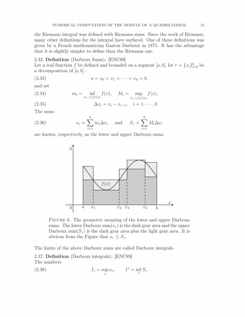
2.32. Definition (Darboux Sums). [ENC89]Let a real function f be defined and bounded on a segment [a, b], let τ = xik
i=0 bea decomposition of [a, b] :
(2.33) a = x0 < x1 < · · · < xk = b,
and set
mi = infxi−1≤x≤xi
f(x), Mi = supxi−1≤x≤xi
f(x),(2.34)
∆xi = xi − xi−1, i = 1, · · · , k.(2.35)
The sums
(2.36) sτ =k∑
i=1
mi∆xi and Sτ =k∑
i=1
Mi∆xi
are known, respectively, as the lower and upper Darboux sums.
0
y
x
f(x)
a x1 x2 x3 x4 b
Figure 6. The geometric meaning of the lower and upper Darbouxsums. The lower Darboux sum(sτ ) is the dark gray area and the upperDarboux sum(Sτ ) is the dark gray area plus the light gray area. It isobvious from the Figure that sτ ≤ Sτ .
The limits of the above Darboux sums are called Darboux integrals.
2.37. Definition (Darboux integrals). [ENC89]The numbers
(2.38) I∗ = supτ
sτ , I∗ = infτ
Sτ
16 JUHANA YRJÖLÄ
are called, respectively, the lower and the upper Darboux integrals of f . They arethe limits of the lower and upper Darboux sums:
(2.39) I∗ = limδτ→0
sτ , I∗ = limδτ→0
Sτ
Where
(2.40) δτ = maxi=1,··· ,k
∆xi.
δτ is called the fineness (mess) of the decomposition.
2.41. Theorem (Riemann and Darboux integrable functions). [ENC89]The necessary and sufficient condition for a function f to be Riemann integrable onthe segment [a, b] is
(2.42) I∗ = I∗.
If the above condition is met, then the value of the lower and the upper Darbouxintegrals becomes identical with the Riemann integral
(2.43)
∫ b
a
f(x)dx.
For the proof of the Theorem see [AB98, pp. 177-187].
2.5. Elliptic integrals.
Many interesting and useful integrals cannot be expressed in terms of elementaryfunctions, such as the length of the rectificated lemniscate, capacitance of an ellip-soid and map of upper half-plane to a rectangle. These integral functions, known asElliptic integrals, were exhaustively studied in 1797-1829 by Gauss, Legendre, Abeland Jacobi. Furthermore they showed that every elliptic integral can be reducedto one of the three normal forms. These normal forms are called elliptic integralof the first, the second and the third kind[MM99, pp. 54-65]. Here we are onlyinterested in elliptic integrals of the first kind because they map upper half-planeto a rectangle.
2.44. Definition (The elliptic integral of the first kind). [MM99, pp. 55-57] [SL99,p. 195]
(2.45) F (k, φ) =
∫ sinφ
0
dv√
(1 − v2)(1 − k2v2),
Where 0 < k < 1, k is called the elliptic modulus and φ is called the amplitude.Also we will denote the complementary elliptic modulus by k′, where k′ =
√1 − k2.
If we are only interested in the borders of the image rectangle we can use simplifiedversion of the elliptic integral F (k, φ). This simplified integral is called the completeelliptic integral of the first kind.
NUMERICAL COMPUTATION OF THE MODULE OF A QUADRILATERAL 17
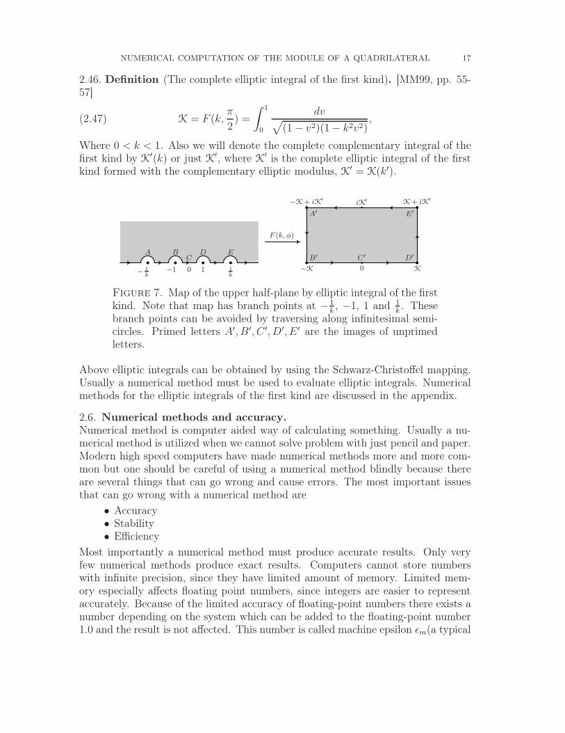
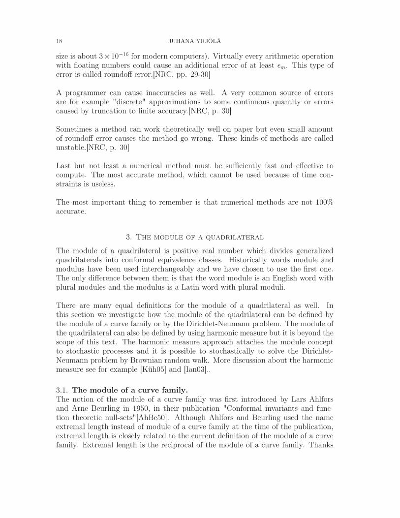
2.46. Definition (The complete elliptic integral of the first kind). [MM99, pp. 55-57]
(2.47) K = F (k,π
2) =
∫ 1
0
dv√
(1 − v2)(1 − k2v2),
Where 0 < k < 1. Also we will denote the complete complementary integral of thefirst kind by K
′(k) or just K′, where K
′ is the complete elliptic integral of the firstkind formed with the complementary elliptic modulus, K
′ = K(k′).
− 1
k−1 0 1 1
k−K 0 K
K+ iK′iK′−K+ iK′
F (k, φ)
B′ C′ D′
E′A′
A BC
D E
Figure 7. Map of the upper half-plane by elliptic integral of the firstkind. Note that map has branch points at − 1
k, −1, 1 and 1
k. These
branch points can be avoided by traversing along infinitesimal semi-circles. Primed letters A′, B′, C ′, D′, E ′ are the images of unprimedletters.
Above elliptic integrals can be obtained by using the Schwarz-Christoffel mapping.Usually a numerical method must be used to evaluate elliptic integrals. Numericalmethods for the elliptic integrals of the first kind are discussed in the appendix.
2.6. Numerical methods and accuracy.
Numerical method is computer aided way of calculating something. Usually a nu-merical method is utilized when we cannot solve problem with just pencil and paper.Modern high speed computers have made numerical methods more and more com-mon but one should be careful of using a numerical method blindly because thereare several things that can go wrong and cause errors. The most important issuesthat can go wrong with a numerical method are
• Accuracy• Stability• Efficiency
Most importantly a numerical method must produce accurate results. Only veryfew numerical methods produce exact results. Computers cannot store numberswith infinite precision, since they have limited amount of memory. Limited mem-ory especially affects floating point numbers, since integers are easier to representaccurately. Because of the limited accuracy of floating-point numbers there exists anumber depending on the system which can be added to the floating-point number1.0 and the result is not affected. This number is called machine epsilon εm(a typical
18 JUHANA YRJÖLÄ
size is about 3×10⁻¹⁶ for modern computers). Virtually every arithmetic operationwith floating numbers could cause an additional error of at least εm. This type oferror is called roundoff error.[NRC, pp. 29-30]
A programmer can cause inaccuracies as well. A very common source of errorsare for example "discrete" approximations to some continuous quantity or errorscaused by truncation to finite accuracy.[NRC, p. 30]
Sometimes a method can work theoretically well on paper but even small amountof roundoff error causes the method go wrong. These kinds of methods are calledunstable.[NRC, p. 30]
Last but not least a numerical method must be sufficiently fast and effective tocompute. The most accurate method, which cannot be used because of time con-straints is useless.
The most important thing to remember is that numerical methods are not 100%accurate.
3. The module of a quadrilateral
The module of a quadrilateral is positive real number which divides generalizedquadrilaterals into conformal equivalence classes. Historically words module andmodulus have been used interchangeably and we have chosen to use the first one.The only difference between them is that the word module is an English word withplural modules and the modulus is a Latin word with plural moduli.
There are many equal definitions for the module of a quadrilateral as well. Inthis section we investigate how the module of the quadrilateral can be defined bythe module of a curve family or by the Dirichlet-Neumann problem. The module ofthe quadrilateral can also be defined by using harmonic measure but it is beyond thescope of this text. The harmonic measure approach attaches the module conceptto stochastic processes and it is possible to stochastically to solve the Dirichlet-Neumann problem by Brownian random walk. More discussion about the harmonicmeasure see for example [Küh05] and [Ian03]..
3.1. The module of a curve family.
The notion of the module of a curve family was first introduced by Lars Ahlforsand Arne Beurling in 1950, in their publication "Conformal invariants and func-tion theoretic null-sets"[AhBe50]. Although Ahlfors and Beurling used the nameextremal length instead of module of a curve family at the time of the publication,extremal length is closely related to the current definition of the module of a curvefamily. Extremal length is the reciprocal of the module of a curve family. Thanks
NUMERICAL COMPUTATION OF THE MODULE OF A QUADRILATERAL 19
to the work of Ahlfors and Beurling, active development of the theory began and al-ready in 1957 Bengt Fuglede generalized their notion and gave it a measure-theoreticinterpretation.[Väi71, p. 20][Vas02, p. 1]
Before we can give the formal definition of module of a curve family we need todefine some auxiliary concepts.
Let ρ(z) be non-negative, real valued, continuous4 and integrable function in somedomain D of C. Now this function ρ(z) defines a differential metric ρ on D byρ := ρ(z)|dz|.3.1. Definition (ρ-length). [Vas02, p. 8]Let D be a domain in C and let γ be a curve in D, then the lower Darboux integral5
(3.2) lρ(γ) =
∫
γ
ρ(z)|dz|
is called the ρ-length of γ. Note that if ρ(z) = 1 almost everywhere and γ isrectifiable, then lρ(γ) is Euclidean length of γ ⊂ D. Let Γ be a family of curves γin D, then the next quantity
(3.3) Lρ(Γ) = infγ∈Γ
lρ(γ)
is called the ρ-length of the curve family Γ.
Reason for the above notation for Lρ(Γ) becomes clear soon, when the definition ofthe module of the curve family is given.
3.4. Definition (ρ-area). [Vas02, p. 8]Let D be a domain in C and let γ be a curve in D, then the integral
(3.5) Aρ(D) =
∫∫
D
ρ2(z)dσz, dσz = dx · dy
is called the ρ-area of D.
3.6. Definition (The module of the curve family). [Vas02, p. 8]Let D be a domain in C and let Γ be a curve family in D, then the quantity
(3.7) m(D, Γ) = infρ
Aρ(D)
L2ρ(Γ)
4Here the continuous requirement is a simplification that we do here, since we have not discussedmeasure theory in the background chapter. The whole theory must be applied to Borel functionsρ(z), which satisfy other conditions given above. However for the module of a quadrilateral com-putations continuous functions are enough[Väi71, p. 20]. Note that all continuous functions areBorel functions but not all Borel functions are continuous.
5Here the lower Darboux integral is chosen so that the integral always exists even if the curve γ
is non-rectifiable, however the curve must be locally rectifiable. This discussion is purely academicsince in the module of a quadrilateral computations we need to restrict to rectifiable curves anyway.See Theorem 3.13.
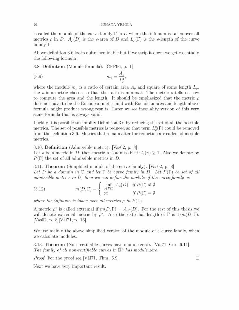
20 JUHANA YRJÖLÄ
is called the module of the curve family Γ in D where the infimum is taken over allmetrics ρ in D. Aρ(D) is the ρ-area of D and Lρ(Γ) is the ρ-length of the curvefamily Γ.
Above definition 3.6 looks quite formidable but if we strip it down we get essentiallythe following formula
3.8. Definition (Module formula). [CFP96, p. 1]
(3.9) mρ =Aρ
L2ρ
,
where the module mρ is a ratio of certain area Aρ and square of some length Lρ.the ρ is a metric chosen so that the ratio is minimal. The metric ρ tells us howto compute the area and the length. It should be emphasized that the metric ρdoes not have to be the Euclidean metric and with Euclidean area and length aboveformula might produce wrong results. Later we see inequality version of this verysame formula that is always valid.
Luckily it is possible to simplify Definition 3.6 by reducing the set of all the possiblemetrics. The set of possible metrics is reduced so that term L2
ρ(Γ) could be removedfrom the Definition 3.6. Metrics that remain after the reduction are called admissiblemetrics.
3.10. Definition (Admissible metric). [Vas02, p. 8]Let ρ be a metric in D, then metric ρ is admissible if lρ(γ) ≥ 1. Also we denote byP (Γ) the set of all admissible metrics in D.
3.11. Theorem (Simplified module of the curve family). [Vas02, p. 8]Let D be a domain in C and let Γ be curve family in D. Let P (Γ) be set of alladmissible metrics in D, then we can define the module of the curve family as
(3.12) m(D, Γ) =
infρ∈P (Γ)
Aρ(D) if P (Γ) 6= ∅∞ if P (Γ) = ∅
where the infimum is taken over all metrics ρ in P (Γ).
A metric ρ∗ is called extremal if m(D, Γ) = Aρ∗(D). For the rest of this thesis wewill denote extremal metric by ρ∗. Also the extremal length of Γ is 1/m(D, Γ).[Vas02, p. 8][Väi71, p. 16]
We use mainly the above simplified version of the module of a curve family, whenwe calculate modules.
3.13. Theorem (Non-rectifiable curves have module zero). [Väi71, Cor. 6.11]The family of all non-rectifiable curves in Rn has module zero.
Proof. For the proof see [Väi71, Thm. 6.9]
Next we have very important result.
NUMERICAL COMPUTATION OF THE MODULE OF A QUADRILATERAL 21
3.14. Theorem (Conformal invariance of the module of a curve family). [Vas02,Thm. 2.1.1]Let Γ be a family of curves in a domain D ∈ C, and let w = f(z) be a conformalmap of D onto D′ ∈ C. If Γ′ = f(Γ), then
(3.15) m(D, Γ) = m(D′, Γ′).
Proof. Let P ′ be the family of all admissible metrics for Γ′ and let P be the familyof admissible metrics for Γ. Let us set ρ(z)|dz| = ρ(f(z))|f ′(z)||dz| for ρ ∈ P ′. Since
(3.16)
∫
γ∈Γ
ρ(z)|dz| =
∫
γ
ρ(f(z))|f ′(z)||dz| =
∫
f(γ)∈Γ′
ρ(w)|dw| ≥ 1,
for any γ ∈ Γ, we have ρ ∈ P . By change of variables under a conformal map in 3.5we have Aρ(D) = Aρ(D
′). Hence,
(3.17) m(D, Γ) = infP
Aρ(D) ≤ infρ∈P
Aρ(D′) = m(D′, Γ′).
Considering the inverse map z = f−1(w) we obtain the reverse inequality and thenthe proof is finished. [Vas02, p. 9]
Next results are good to keep in mind when trying to calculate the module of thecurve family.
3.18. Theorem (Properties of the extremal metric). [Vas02, Thms. 2.1.2-2.1.3]
(i) (Uniqueness of the extremal metric):Let ρ∗
1 and ρ∗2 be two extremal metrics for the module m(D, Γ),
then ρ∗ = ρ∗1 = ρ∗
2 almost everywhere.
(ii) (ρ∗-length of the curve family Γ):Lρ∗(Γ) = 1
(iii) (Monotonicity):If Γ1 ⊂ Γ2 in D, then m(D, Γ1) ≤ m(D, Γ2).
Proof. (i) Since ρ1 and ρ2 are extremal metrics for the module m(D, Γ), they areadmissible. Then 1
2(ρ1(z) + ρ2(z))|dz| is an admissible metric, and
(3.19)
∫∫
D
(ρ1(z) + ρ2(z)
2
)2
dσz ≥ m(D, Γ).
22 JUHANA YRJÖLÄ
We have the chain of inequalities
0 ≤∫∫
D
(ρ1(z) − ρ2(z)
2
)2
dσz(3.20)
=
∫∫
D
(ρ21(z) + ρ2
2(z)
2
)
dσz −∫∫
D
(ρ1(z) + ρ2(z)
2
)2
dσz(3.21)
= m(D, Γ) −∫∫
D
(ρ1(z) + ρ2(z)
2
)2
dσz ≤ 0,(3.22)
which is valid only if ρ1(z) = ρ2(z) almost everywhere. [Vas02, p. 9]
(ii) We denote by ρ∗(z)|dz| this extremal metric. Suppose that Lρ∗(Γ) = c > 1.Then the metric 1
cρ∗(z)|dz| is admissible and
(3.23) m(D, Γ) ≤ 1
c2
∫∫
D
(ρ∗(z))2dσz =1
c2m(D, Γ) < m(D, Γ)
This is a contradiction, proving (ii). [Vas02, p. 9]
(iii) This follows from the inequality Lρ(Γ1) ≥ Lρ(Γ2).[Vas02, p. 10]
Now it is time to investigate the connection between the module of a curve familyand the module of a quadrilateral. These concepts are not completely the same,since the module of a curve family is a more general concept.
3.24. Definition (Module of a quadrilateral). [Küh05, p. 107]Let Q be a quadrilateral with four vertices z1, z2, z3 and z4. Let τ1 and τ2 be twoopposite sides of the quadrilateral and let Γ1 be a curve family of all rectifiablecurves that connect the two opposite sides τ1 and τ2 of Q. Then the module of aquadrilateral Q(z1, z2, z3, z4) with τ1 and τ2 as opposite sides is the module of thecurve family Γ1.
We denote the module of a quadrilateral with capital M, in contrast to the lowercase m, which denotes the module of a curve family. Also note that since the mod-ule of a curve family is conformal invariant by Theorem 3.14 then the module of aquadrilateral is also a conformal invariant.
If we replace the opposite sides τ1 and τ2 of Q by the other set of opposite sidesthen module of the quadrilateral Q is equal to reciprocal module 1/M(Q).[Küh05,p. 101] If we do not take all the curves that connect opposite sides of Q then weget following inequality
(3.25) m(Q, Γ) ≤ M(Q),
NUMERICAL COMPUTATION OF THE MODULE OF A QUADRILATERAL 23
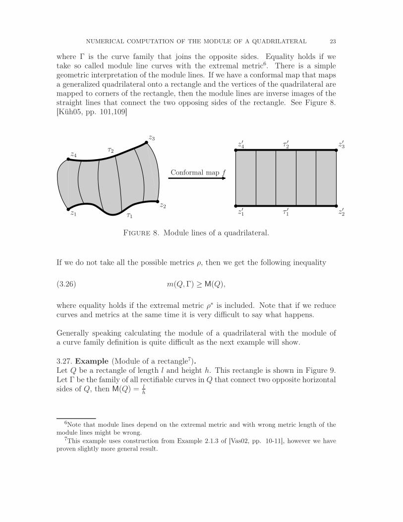
where Γ is the curve family that joins the opposite sides. Equality holds if wetake so called module line curves with the extremal metric6. There is a simplegeometric interpretation of the module lines. If we have a conformal map that mapsa generalized quadrilateral onto a rectangle and the vertices of the quadrilateral aremapped to corners of the rectangle, then the module lines are inverse images of thestraight lines that connect the two opposing sides of the rectangle. See Figure 8.[Küh05, pp. 101,109]
z1
z2
z3
z4
z′1 z′2
z′3z′4
τ1
τ2
τ ′1
τ ′2
Conformal map f
Figure 8. Module lines of a quadrilateral.
If we do not take all the possible metrics ρ, then we get the following inequality
(3.26) m(Q, Γ) ≥ M(Q),
where equality holds if the extremal metric ρ∗ is included. Note that if we reducecurves and metrics at the same time it is very difficult to say what happens.
Generally speaking calculating the module of a quadrilateral with the module ofa curve family definition is quite difficult as the next example will show.
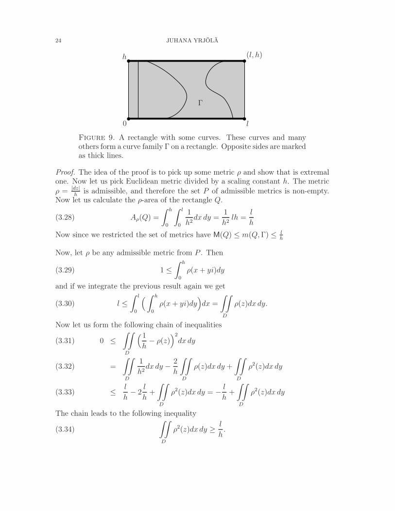
3.27. Example (Module of a rectangle7).Let Q be a rectangle of length l and height h. This rectangle is shown in Figure 9.Let Γ be the family of all rectifiable curves in Q that connect two opposite horizontalsides of Q, then M(Q) = l
h
6Note that module lines depend on the extremal metric and with wrong metric length of themodule lines might be wrong.
7This example uses construction from Example 2.1.3 of [Vas02, pp. 10-11], however we haveproven slightly more general result.
24 JUHANA YRJÖLÄ
0 l
h (l, h)
Γ
Figure 9. A rectangle with some curves. These curves and manyothers form a curve family Γ on a rectangle. Opposite sides are markedas thick lines.
Proof. The idea of the proof is to pick up some metric ρ and show that is extremalone. Now let us pick Euclidean metric divided by a scaling constant h. The metric
ρ = |dz|h
is admissible, and therefore the set P of admissible metrics is non-empty.Now let us calculate the ρ-area of the rectangle Q.
(3.28) Aρ(Q) =
∫ h
0
∫ l
0
1
h2dx dy =
1
h2lh =
l
h
Now since we restricted the set of metrics have M(Q) ≤ m(Q, Γ) ≤ lh
Now, let ρ be any admissible metric from P . Then
(3.29) 1 ≤∫ h
0
ρ(x + yi)dy
and if we integrate the previous result again we get
(3.30) l ≤∫ l
0
(
∫ h
0
ρ(x + yi)dy)
dx =
∫∫
D
ρ(z)dx dy.
Now let us form the following chain of inequalities
0 ≤∫∫
D
(1
h− ρ(z)
)2
dx dy(3.31)
=
∫∫
D
1
h2dx dy − 2
h
∫∫
D
ρ(z)dx dy +
∫∫
D
ρ2(z)dx dy(3.32)
≤ l
h− 2
l
h+
∫∫
D
ρ2(z)dx dy = − l
h+
∫∫
D
ρ2(z)dx dy(3.33)
The chain leads to the following inequality
(3.34)
∫∫
D
ρ2(z)dx dy ≥ l
h.
NUMERICAL COMPUTATION OF THE MODULE OF A QUADRILATERAL 25
for any admissible ρ and, taking the infimum over all ρ, we have M(Q) = m(Q, Γ) ≥ lh.
Now since lh≤ M(Q) ≤ l
hwe see that
(3.35) M(Q) =l
h
Note that the module of a quadrilateral for a rectangle is the aspect ratio of therectangle. Also note that if we switch the opposite sides of Q, then we get thereciprocal module h
l
Since the exact calculation of the module of the quadrilateral is very difficult andtiresome, inequalities have a major role in getting estimates for the modules.
3.36. Theorem (Rengel’s inequality). [LV73, p. 22]The module of a quadrilateral Q satisfies the double inequality
(3.37)(Lρ(Γ
′))2
Aρ
≤ M(Q) ≤ Aρ
(Lρ(Γ))2.
Where Γ′ and Γ are curve families that connect the opposite sides of a quadrilateralQ. Equality holds in both cases when and only when Q is a rectangle.
Proof. For the proof see [LV73, pp. 22-23]
Note that the Rengel’s inequality is inequality version of the formula (3.9)8.
3.2. The Dirichlet-Neumann problem and the module of a quadrilateral.
There is another definition for the module of a quadrilateral, which is based onLaplace’s equation on a rectangle. This formulation actually gives us three differ-ent definitions. Namely definitions that are based on Laplace’s equation, geometricshape of the quadrilateral and capacitance of a condenser. All these definitions arevery closely related as we are about to see.
First we take a look at the Dirichlet-Neumann formulation for the module of aquadrilateral. It should be emphasized that the Dirichlet-integral given below isindeed a conformal invariant, although we do not prove it here. The proof was giveby Loewner in 1959, see [Loe59].
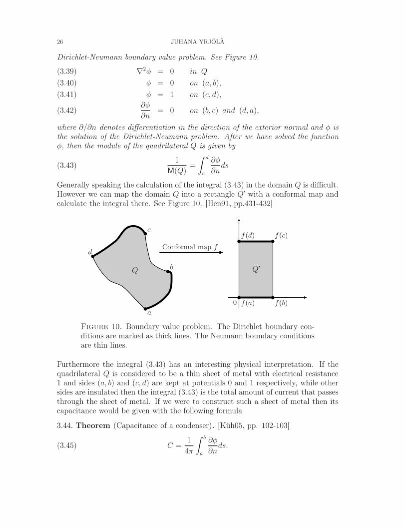
3.38. Theorem (Dirichlet-Neumann definition). [Hen91, pp.431-432]Let Q be a quadrilateral with vertices a, b, c, d and edges (a, b), (b, c), (c, d),(d, a). Now the module of a quadrilateral can be determined by solving the following
8It is also possible to estimate the module of a quadrilateral with two Euclidean lengths and noinformation about the area. See [LV73, p. 23].
26 JUHANA YRJÖLÄ
Dirichlet-Neumann boundary value problem. See Figure 10.
∇2φ = 0 in Q(3.39)
φ = 0 on (a, b),(3.40)
φ = 1 on (c, d),(3.41)
∂φ
∂n= 0 on (b, c) and (d, a),(3.42)
where ∂/∂n denotes differentiation in the direction of the exterior normal and φ isthe solution of the Dirichlet-Neumann problem. After we have solved the functionφ, then the module of the quadrilateral Q is given by
(3.43)1
M(Q)=
∫ d
c
∂φ
∂nds
Generally speaking the calculation of the integral (3.43) in the domain Q is difficult.However we can map the domain Q into a rectangle Q′ with a conformal map andcalculate the integral there. See Figure 10. [Hen91, pp.431-432]
a
d
c
bQ
Conformal map f
0 f(a) f(b)
f(c)f(d)
Q′
Figure 10. Boundary value problem. The Dirichlet boundary con-ditions are marked as thick lines. The Neumann boundary conditionsare thin lines.
Furthermore the integral (3.43) has an interesting physical interpretation. If thequadrilateral Q is considered to be a thin sheet of metal with electrical resistance1 and sides (a, b) and (c, d) are kept at potentials 0 and 1 respectively, while othersides are insulated then the integral (3.43) is the total amount of current that passesthrough the sheet of metal. If we were to construct such a sheet of metal then itscapacitance would be given with the following formula
3.44. Theorem (Capacitance of a condenser). [Küh05, pp. 102-103]
(3.45) C =1
4π
∫ b
a
∂φ
∂nds.
NUMERICAL COMPUTATION OF THE MODULE OF A QUADRILATERAL 27
Also if we do know the module of any quadrilateral, then we can compute thecapacitance of that quadrilateral with following module-capacitance formula.
3.46. Theorem (Module-capacitance formula9). [Gai79, p. 236]Let M(Q) be the module of the quadrilateral Q with vertices a, b, c and d. Then thecapacitance between the sides (a, b) and (c, d) is given by
(3.47) C =1
π2
∑
n=odd
1
n sinh (nπM(Q))
Since the module of a quadrilateral is invariant under conformal mappings we cansimplify the Dirichlet-Neumann domain by a conformal mapping. Because we al-ready know how to compute the module of a rectangle (See Example 3.27), thena conformal map to a rectangle gives us the following geometric definition for themodule of a quadrilateral.
3.48. Definition (Geometric definition). [Küh05, p. 101]Let Q be a quadrilateral with vertices a, b, c and d. Let f be a conformal map thatmaps Q into a rectangle and vertices a, b, c and d map into corners of that rectangleso that vertex a maps to zero and vertex b maps on a real axis. See Figure 10. Thenthe module of Q is given by
(3.49) M(Q) =Im f(c)
Re f(b)=
height
length
where Im f(c) is the imaginary part of f(c) and Re f(b) is the real part of f(b).
The only problem with this geometric definition is that it requires a construction ofa conformal map that maps a quadrilateral into a rectangle. In the next section weare going to look at how this map could be constructed for polygonal quadrilaterals.
4. The Schwarz-Christoffel Mapping
In 1851 the German mathematician Bernhard Riemann presented in his doctoraldissertation the famous Riemann’s mapping theorem that guarantees that any sim-ply connected domain in the complex plane can be mapped to some other simplyconnected domain by a conformal mapping. However Riemann’s theorem is an exis-tence Theorem only and it does not give the required mapping function. Soon afterthe Riemann’s discovery, Elwin Christoffel(1867) and Hermann Schwarz (1869) in-dependently discovered the Riemann mapping function in a case where the range ofthe mapping domain is a polygon. This mapping is called the Schwarz-Christoffelmapping.[Fla83][Dri02]
9Matlab implementation of this algorithm is given in the Schwarz-Christoffel toolbox section.
28 JUHANA YRJÖLÄ
D D′
z1 z2 z3 z4 z5
w1
w2 w3
w4
w5
w plane
Schwarz-Christoffel polygon
z plane
y
x
v
u
α1
α2
α3
α4
α5
Schwarz-Christoffelmapping
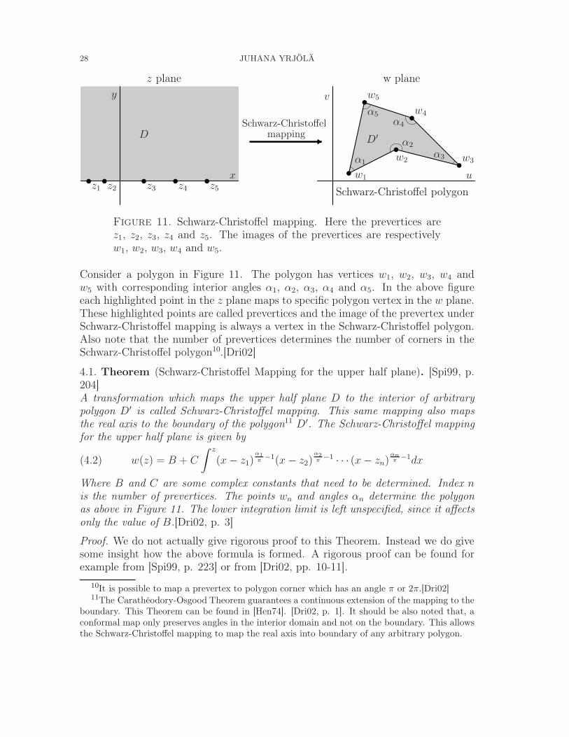
Figure 11. Schwarz-Christoffel mapping. Here the prevertices arez1, z2, z3, z4 and z5. The images of the prevertices are respectivelyw1, w2, w3, w4 and w5.
Consider a polygon in Figure 11. The polygon has vertices w1, w2, w3, w4 andw5 with corresponding interior angles α1, α2, α3, α4 and α5. In the above figureeach highlighted point in the z plane maps to specific polygon vertex in the w plane.These highlighted points are called prevertices and the image of the prevertex underSchwarz-Christoffel mapping is always a vertex in the Schwarz-Christoffel polygon.Also note that the number of prevertices determines the number of corners in theSchwarz-Christoffel polygon10.[Dri02]
4.1. Theorem (Schwarz-Christoffel Mapping for the upper half plane). [Spi99, p.204]A transformation which maps the upper half plane D to the interior of arbitrarypolygon D′ is called Schwarz-Christoffel mapping. This same mapping also mapsthe real axis to the boundary of the polygon11 D′. The Schwarz-Christoffel mappingfor the upper half plane is given by
(4.2) w(z) = B + C
∫ z
(x − z1)α1π−1(x − z2)
α2π
−1 · · · (x − zn)αnπ
−1dx
Where B and C are some complex constants that need to be determined. Index nis the number of prevertices. The points wn and angles αn determine the polygonas above in Figure 11. The lower integration limit is left unspecified, since it affectsonly the value of B.[Dri02, p. 3]
Proof. We do not actually give rigorous proof to this Theorem. Instead we do givesome insight how the above formula is formed. A rigorous proof can be found forexample from [Spi99, p. 223] or from [Dri02, pp. 10-11].
10It is possible to map a prevertex to polygon corner which has an angle π or 2π.[Dri02]11The Carathéodory-Osgood Theorem guarantees a continuous extension of the mapping to the
boundary. This Theorem can be found in [Hen74]. [Dri02, p. 1]. It should be also noted that, aconformal map only preserves angles in the interior domain and not on the boundary. This allowsthe Schwarz-Christoffel mapping to map the real axis into boundary of any arbitrary polygon.
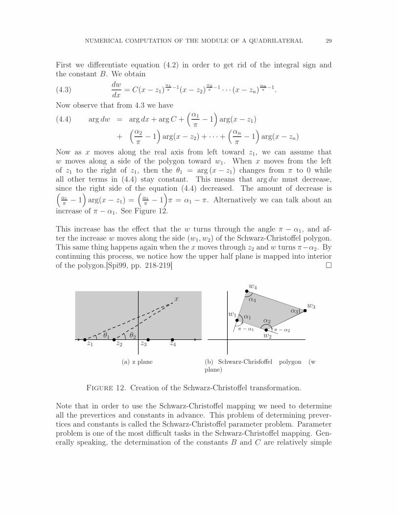
NUMERICAL COMPUTATION OF THE MODULE OF A QUADRILATERAL 29
First we differentiate equation (4.2) in order to get rid of the integral sign andthe constant B. We obtain
(4.3)dw
dx= C(x − z1)
α1π−1(x − z2)
α2π−1 · · · (x − zn)
αnπ
−1.
Now observe that from 4.3 we have
arg dw = arg dx + arg C +(α1
π− 1)
arg(x − z1)(4.4)
+(α2
π− 1)
arg(x − z2) + · · ·+(αn
π− 1)
arg(x − zn)
Now as x moves along the real axis from left toward z1, we can assume thatw moves along a side of the polygon toward w1. When x moves from the leftof z1 to the right of z1, then the θ1 = arg (x − z1) changes from π to 0 whileall other terms in (4.4) stay constant. This means that arg dw must decrease,since the right side of the equation (4.4) decreased. The amount of decrease is(
α1
π− 1)
arg(x − z1) =(
α1
π− 1)
π = α1 − π. Alternatively we can talk about an
increase of π − α1. See Figure 12.
This increase has the effect that the w turns through the angle π − α1, and af-ter the increase w moves along the side (w1, w2) of the Schwarz-Christoffel polygon.This same thing happens again when the x moves through z2 and w turns π−α2. Bycontinuing this process, we notice how the upper half plane is mapped into interiorof the polygon.[Spi99, pp. 218-219]
z1 z2 z3 z4
x
θ1 θ2
(a) z plane
w1
w2
w3
w4
α1 α2
α3
α4
π − α1 π − α2
(b) Schwarz-Chrisfoffel polygon (wplane)
Figure 12. Creation of the Schwarz-Christoffel transformation.
Note that in order to use the Schwarz-Christoffel mapping we need to determineall the prevertices and constants in advance. This problem of determining prever-tices and constants is called the Schwarz-Christoffel parameter problem. Parameterproblem is one of the most difficult tasks in the Schwarz-Christoffel mapping. Gen-erally speaking, the determination of the constants B and C are relatively simple
30 JUHANA YRJÖLÄ
after the prevertices have been determined. Usually a numerical scheme must beused to determine the prevertices.[Dri02, pp. 23-40]
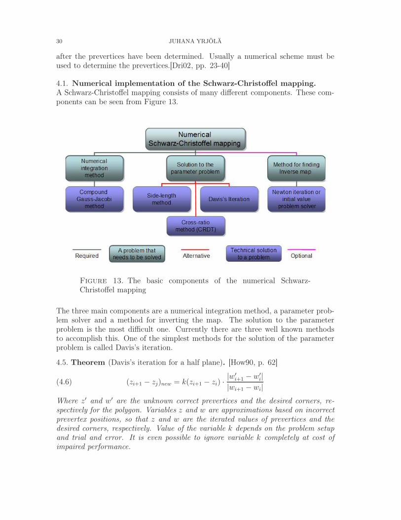
4.1. Numerical implementation of the Schwarz-Christoffel mapping.
A Schwarz-Christoffel mapping consists of many different components. These com-ponents can be seen from Figure 13.
Figure 13. The basic components of the numerical Schwarz-Christoffel mapping
The three main components are a numerical integration method, a parameter prob-lem solver and a method for inverting the map. The solution to the parameterproblem is the most difficult one. Currently there are three well known methodsto accomplish this. One of the simplest methods for the solution of the parameterproblem is called Davis’s iteration.
4.5. Theorem (Davis’s iteration for a half plane). [How90, p. 62]
(4.6) (zi+1 − zj)new = k(zi+1 − zi) ·|w′
i+1 − w′i|
|wi+1 − wi|Where z′ and w′ are the unknown correct prevertices and the desired corners, re-spectively for the polygon. Variables z and w are approximations based on incorrectprevertex positions, so that z and w are the iterated values of prevertices and thedesired corners, respectively. Value of the variable k depends on the problem setupand trial and error. It is even possible to ignore variable k completely at cost ofimpaired performance.
NUMERICAL COMPUTATION OF THE MODULE OF A QUADRILATERAL 31
Davis’s iteration is computationally cheap (compared to other methods) and simpleto implement. Because of its cheap computation time, it has been used to solve theparameter problem for polygons with thousand or more vertices[BT03]. However H.Howell pointed out that Davis’s iteration is not the best way to solve the parameterproblem for the following reasons:
• Parameters for the Davis’s iteration change case-by-case basis(namely k).Determining the right ones for the problem at hand is often impractical.
• Many Schwarz-Christoffel problems have additional conditions to be satis-fied. For example if the conformal module is known and one polygonal sidelength is left unspecified. To accomplish this with Davis’s iteration is hard.
• Convergence rate near the solution is only linear.• The most critical fact is that Davis’s iteration might not converge at all.
For more details see[How90, p. 62-64].
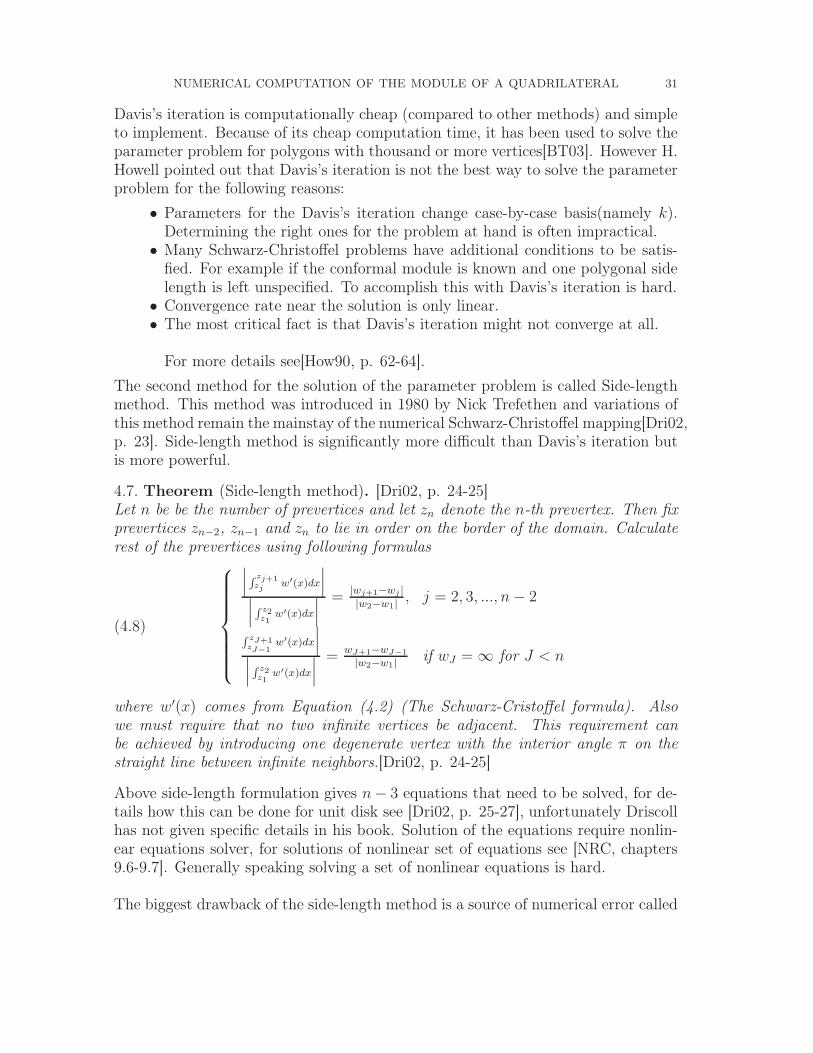
The second method for the solution of the parameter problem is called Side-lengthmethod. This method was introduced in 1980 by Nick Trefethen and variations ofthis method remain the mainstay of the numerical Schwarz-Christoffel mapping[Dri02,p. 23]. Side-length method is significantly more difficult than Davis’s iteration butis more powerful.
4.7. Theorem (Side-length method). [Dri02, p. 24-25]Let n be be the number of prevertices and let zn denote the n-th prevertex. Then fixprevertices zn−2, zn−1 and zn to lie in order on the border of the domain. Calculaterest of the prevertices using following formulas
(4.8)
∣
∣
∣
R zj+1zj
w′(x)dx
∣
∣
∣
∣
∣
∣
R z2z1
w′(x)dx
∣
∣
∣
=|wj+1−wj |
|w2−w1|, j = 2, 3, ..., n − 2
R zJ+1zJ−1
w′(x)dx
∣
∣
∣
∣
∣
∣
R z2z1
w′(x)dx
∣
∣
∣
= wJ+1−wJ−1
|w2−w1|if wJ = ∞ for J < n
where w′(x) comes from Equation (4.2) (The Schwarz-Cristoffel formula). Alsowe must require that no two infinite vertices be adjacent. This requirement canbe achieved by introducing one degenerate vertex with the interior angle π on thestraight line between infinite neighbors.[Dri02, p. 24-25]
Above side-length formulation gives n − 3 equations that need to be solved, for de-tails how this can be done for unit disk see [Dri02, p. 25-27], unfortunately Driscollhas not given specific details in his book. Solution of the equations require nonlin-ear equations solver, for solutions of nonlinear set of equations see [NRC, chapters9.6-9.7]. Generally speaking solving a set of nonlinear equations is hard.
The biggest drawback of the side-length method is a source of numerical error called
32 JUHANA YRJÖLÄ
crowding. Crowding is present in almost all numerical conformal mapping tech-niques. It should be also noted that above Davis’s iteration suffers from crowdingtoo. Crowding occurs when two prevertices come too close to each other. Because ofthe limited numerical floating point accuracy it might be numerically impossible toeven distinguish two different prevertices. Crowding especially affects regions withlong and thin areas, like a long rectangles. [Dri02, p. 20-21]
For some time thin long regions were a problem and special domain decompositionmethods were developed to combat crowding[Dri02, p. 21]. What is more interestingfrom our point of view is that Papamichael and Stylianopoulos developed domaindecomposition methods especially for module computations, for further details see[PS88],[PS92] and [PS99]. The biggest drawback of these domain decompositionmethods for module computations are that they only give approximate values.
Because of the ill-effects of the crowding to the numerical Schwarz-Cristoffel map-ping Driscoll and Vavasis developed Cross-ratios and Delaunay Triangulations methodfor solving the Schwarz-Cristoffel parameter problem. This method is currentlythe state of the art in numerical Schwarz-Cristoffel mapping. Driscoll and Vava-sis believe that CRDT(Cross-ratios and Delaunay Triangulations)-method removescrowding completely and solves convergence problems. This method is too lengthyto be described here, for details see [DV98] and [Dri02, p. 30-39].
Although Driscoll and Vavasis have developed a very good method, it is very difficultand requires lots of hard work to implement it. Luckily Driscoll has implementedthis method as well as side-length method in Matlab toolbox called "Schwarz-Christoffel Toolbox" and made it available for free. We will look at Driscoll’sSchwarz-Christoffel toolbox later.
Any numerical implementation of the Schwarz-Christoffel mapping needs a numer-ical integration method. Although almost any numerical integration method canbe used, the Schwarz-Christoffel integral is often singular at prevertices and con-ventional methods perform poorly. The current state of the art integration methodfor the Schwarz-Christoffel mapping is the so called compound Gauss-Jacobi quad-rature. This integration method takes account singularities at both endpoints andsingularities near integration interval. The details of this integration method aretoo lengthy to be described here, for additional information see [Dri02, p. 27-29] forgeneral information for the Schwarz-Christoffel integral and see [NRC, p. 147-161]for the evaluation of the Gauss-Jacobi quadrature. Implementation of this inte-gration method is much more complex than Simpson’s method or even Gaussian-Quadrature.
NUMERICAL COMPUTATION OF THE MODULE OF A QUADRILATERAL 33
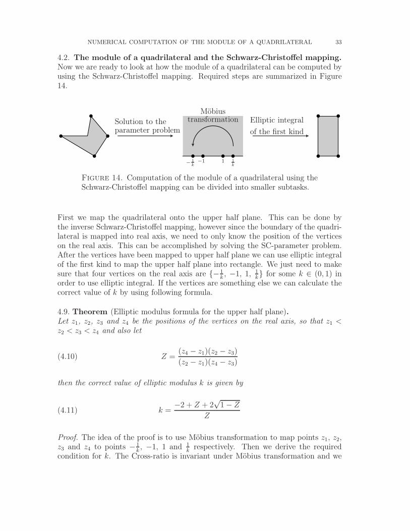
4.2. The module of a quadrilateral and the Schwarz-Christoffel mapping.
Now we are ready to look at how the module of a quadrilateral can be computed byusing the Schwarz-Christoffel mapping. Required steps are summarized in Figure14.
Solution to theparameter problem
Elliptic integral
of the first kind
Möbiustransformation
− 1
k−1 1 1
k
Figure 14. Computation of the module of a quadrilateral using theSchwarz-Christoffel mapping can be divided into smaller subtasks.
First we map the quadrilateral onto the upper half plane. This can be done bythe inverse Schwarz-Christoffel mapping, however since the boundary of the quadri-lateral is mapped into real axis, we need to only know the position of the verticeson the real axis. This can be accomplished by solving the SC-parameter problem.After the vertices have been mapped to upper half plane we can use elliptic integralof the first kind to map the upper half plane into rectangle. We just need to makesure that four vertices on the real axis are − 1
k, −1, 1, 1
k for some k ∈ (0, 1) in
order to use elliptic integral. If the vertices are something else we can calculate thecorrect value of k by using following formula.
4.9. Theorem (Elliptic modulus formula for the upper half plane).Let z1, z2, z3 and z4 be the positions of the vertices on the real axis, so that z1 <z2 < z3 < z4 and also let
(4.10) Z =(z4 − z1)(z2 − z3)
(z2 − z1)(z4 − z3)
then the correct value of elliptic modulus k is given by
(4.11) k =−2 + Z + 2
√1 − Z
Z
Proof. The idea of the proof is to use Möbius transformation to map points z1, z2,z3 and z4 to points − 1
k, −1, 1 and 1
krespectively. Then we derive the required
condition for k. The Cross-ratio is invariant under Möbius transformation and we
34 JUHANA YRJÖLÄ
get
Z =(z4 − z1)(z2 − z3)
(z2 − z1)(z4 − z3)=
(w4 − w1)(w2 − w3)
(w2 − w1)(w4 − w3)(4.12)
=( 1
k+ 1
k)(−1 − 1)
(−1 + 1k)( 1
k− 1)
(4.13)
=−4k
(1 − k)2= Z.(4.14)
We get the following equation from (4.14)
(4.15) Zk2 + k(4 − 2Z) + Z = 0.
By using the quadratic formula we get
(4.16) k =−2 + Z ± 2
√1 − Z
ZNote that Z is always negative when z1 < z2 < z3 < z4, so the solution is realvalued. Also note that the roots are reciprocal values of each other12. Since we needto restrict the values of k such that 1
k> 1. We need to select the smallest value of
k and this happens with + sign in equation (4.16).
When the elliptic modulus k is known we can calculate the module of a quadrilateralby using complete elliptic integrals of the first kind.
4.17. Theorem (Module of a quadrilateral and complete elliptic integrals). [Dri02,p. 19]Let Q be a quadrilateral and let k be the elliptic modulus of Q then
(4.18) M(Q) =K
′(k)
2K(k),
where K is the complete elliptic integral of the first kind and K′ = K(
√1 − k2). See
Figure 7 for the derivation of this result.
Now if the Q is the upper half plane, then we can easily calculate the value ofk by using Theorem 4.9. Since it is relatively simple to calculate the module ofa quadrilateral after we have mapped the quadrilateral into the upper half plane,therefore the most challenging problem is the solution to the parameter problem.See Appendix for numerical evaluation of the elliptic integrals of the first kind.
12Proof:(
−2+Z+2√
1−ZZ
)(
−2+Z−2√
1−ZZ
)
= (−2+Z)2−4(1−Z)Z2 = 4−4Z+Z2
−4+4ZZ2 = 1
NUMERICAL COMPUTATION OF THE MODULE OF A QUADRILATERAL 35
4.3. The Schwarz-Christoffel toolbox.
The Schwarz-Christoffel Toolbox is a Schwarz-Christoffel mapping software for Mat-lab by Tobin A. Driscoll. This toolbox can be downloaded from Driscoll’s home pageat
http://www.math.udel.edu/~driscoll/SC/.
We use the toolbox to calculate the module of quadrilaterals and next we present abrief tutorial on how to use the toolbox for this purpose.
Installation of the toolbox is straight forward, just unpack the files into directoryof your choice and then add that directory to Matlab’s path. This can be accom-plished by the following Matlab command, provided that the toolbox is installed in/sc directory.
path(path,’/sc’)
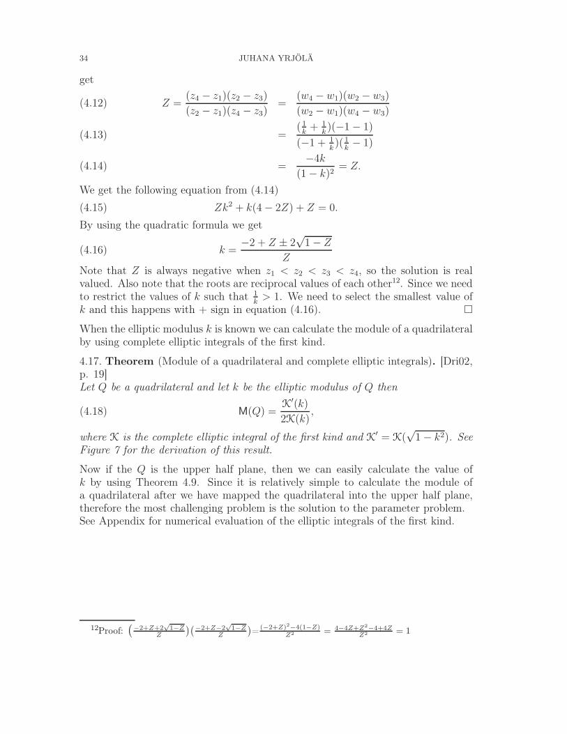
After the path is set the toolbox is ready for use. Toolbox contains both graphicaland command line user interface. Graphical user interface(GUI) can be launchedby typing scgui
(a) Main view (b) Polygon editor (c) Main view with the map
Figure 15. Screenshots from the graphical user interface of Schwarz-Christoffel Toolbox
Almost all functionality of the Schwarz-Christoffel Toolbox can be accessed throughthe graphical user interface, including creation of polygons(Figure 15(b)), selectingthe domain to which the polygon is mapped and exporting data to Matlab’s com-mand line. It is important however to notice, that the toolbox GUI does not givemodule of the quadrilateral directly, although it is clearly visible from the final mapscreen (see Figure 15(c)).[SCTUG]
In this short tutorial we only concentrate on command line interface because itis more flexible and slightly harder to use. First we need to define the polygon,which we want to map. This can be done with polygon command. The followingcode will create polygon with vertices at 0, 4, 3 + 2i and 5 + 5i. This polygon isthen stored in variable p for later use.
36 JUHANA YRJÖLÄ
p=polygon([0 4 3+2i 5+5i])
If we want more or different vertices we just replace or add vertices in complexrepresentation in the list. The toolbox extends some of the most common Matlabfunctions(plot,eval,inv, etc.) to allow easy co-operation with the toolbox’s features.So we could draw a picture of our polygon with plot(p) command. Next we needto define what kind of map we want to use. In the Schwarz-Christoffel Toolboxone selects the type of the map with the function call. We are mainly interestedin rectangle maps because we know how to compute the module of a rectangle.The toolbox contains two different types of rectangle maps namely rectmap andcrrectmap.
rectmap(p)
crrectmap(p)
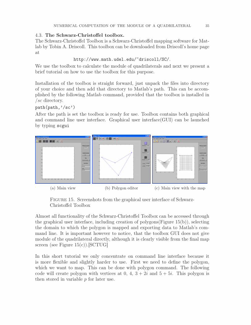
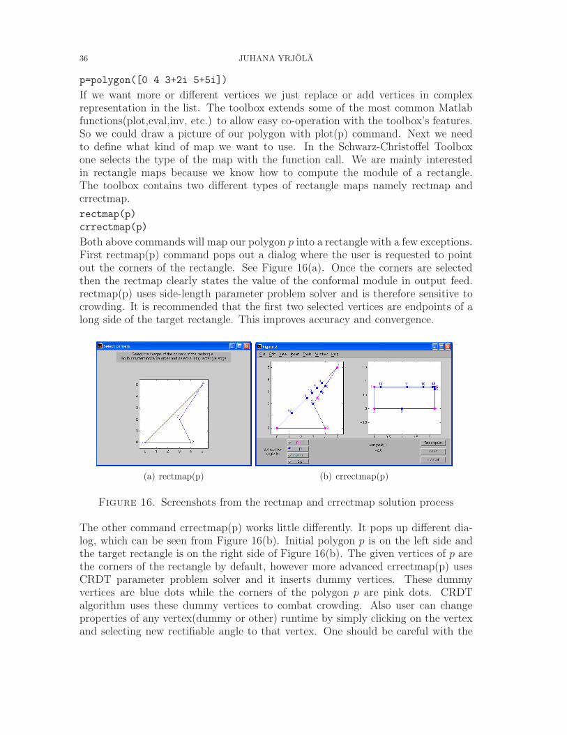
Both above commands will map our polygon p into a rectangle with a few exceptions.First rectmap(p) command pops out a dialog where the user is requested to pointout the corners of the rectangle. See Figure 16(a). Once the corners are selectedthen the rectmap clearly states the value of the conformal module in output feed.rectmap(p) uses side-length parameter problem solver and is therefore sensitive tocrowding. It is recommended that the first two selected vertices are endpoints of along side of the target rectangle. This improves accuracy and convergence.
(a) rectmap(p) (b) crrectmap(p)
Figure 16. Screenshots from the rectmap and crrectmap solution process
The other command crrectmap(p) works little differently. It pops up different dia-log, which can be seen from Figure 16(b). Initial polygon p is on the left side andthe target rectangle is on the right side of Figure 16(b). The given vertices of p arethe corners of the rectangle by default, however more advanced crrectmap(p) usesCRDT parameter problem solver and it inserts dummy vertices. These dummyvertices are blue dots while the corners of the polygon p are pink dots. CRDTalgorithm uses these dummy vertices to combat crowding. Also user can changeproperties of any vertex(dummy or other) runtime by simply clicking on the vertexand selecting new rectifiable angle to that vertex. One should be careful with the
NUMERICAL COMPUTATION OF THE MODULE OF A QUADRILATERAL 37
order of the vertices when changing vertices types, since the order of the verticesin the target polygon is determined by the vertex number and nothing else. Vertexnumbering affects the Dirichlet-Neumann boundary conditions and different bound-ary conditions might give different results. When the changes are ready new map iscomputed by pressing recompute button. Done button finishes the map and returncrrectmap object to command line. The biggest problem with crrectmap is thatmodule is not clearly stated even if it is clearly visible from the picture.
Usually graphical observations are not enough and we want the most "exact" valueof module to some variable for further study. The method how to do this varies withmapping function. Rectmap is simpler than crrectmap, since SC-toolbox computesits module directly. We just need to call the special modulus function to get thenumerical value.
modulus(rectmap(p))
Crrectmap is more complicated since above modulus() function is not compatiblewith it. However we can create following Matlab function that computes the moduleof crrectmap objects.
Matlab function 1 Computation of the module of a quadrilateral for crrectmapobjects
function mo = moduluscr(map)
%Computes the module of crrectmap objects
%map = mapping crrectmap object
pl2=get(map,’rectpolygon’);
angpl=pl2.angle();
angpl=angpl-1;
Ipl=find(angpl);
v=[pl2.vertex(Ipl(1)) pl2.vertex(Ipl(2)) pl2.vertex(Ipl(3)) pl2.vertex(Ipl(4))];
mo=(max(imag(v)) - min(imag(v)))/(max(real(v)) - min(real(v)));
Once the moduluscr()-function has been created we can use it almost identically tomodulus()-function, for example
moduluscr(crrectmap(p))
However popping dialog windows are impractical in the long run, since they requirehuman interaction. We can get rid of the dialogs by giving extra parameters torectmap()- and crrectmap()-functions. To accomplish this rectmap wants a list ofvertex numbers, which are the corners of the target rectangle, as an extra input.On the other hand crrectmap takes a list of angles of the target rectangle at givenvertex position. For example for polygon p
rectmap(p,[2 3 4 1])
crrectmap(p,[0.5 0.5 0.5 0.5])
38 JUHANA YRJÖLÄ
Note that numbering of rectmap vertices is not [1 2 3 4]. This is because of ourdefinition of module of a quadrilateral. We have chosen modulus(rectmap(p,[2 34 1])) to be the module of p while modulus(rectmap(p,[1 2 3 4])) is the reciprocalvalue of the module of p.
Sometimes it is necessary to know the numerical accuracy of the map. This can beaccomplished with accuracy-function as follows.
accuracy(rectmap(p,[2 3 4 1]))
accuracy(crrectmap(p,[0.5 0.5 0.5 0.5]))
Note that accuracy-function is polymorphic, so that same function applies to dif-ferent types of maps.
The next Matlab function calculates the capacitance of the condenser, once themodule of the quadrilateral is known. Algorithm uses the formula (3.47).
Matlab function 2 Computation of the capacitance of the quadrilateral
function cap=capacitance(M,tol)
%Calculates the capacitance of a condenser
%M = The modulus of a quadrilateral
%tol = Tolerance
n=1;
sumvalue=0;
increment=0;
if (M>0)
while ((increment>tol) || (n<50) )
increment=1/(n*sinh(n*pi*M));
sumvalue=sumvalue+increment;
n=n+2;
end
end
cap=(1/(pi^2))*sumvalue;
Unfortunately there is a small bug in the version 2.3 of Schwarz-Christoffel Tool-box, which complicates computations a little bit. Evidently graphical dialogs causecrrectmap to crash in some cases, these cases are not common but in a large batchthey are very likely. There are two known solutions to this problem. First solutionis to write crrectmap call in try catch block so that if the crrectmap returns an errorthen let rectmap do the computations in the catch block, this usually works but isonly recommended as last resort, since rectmap is not as accurate as crrectmap.The second better way is to disable all graphical dialogs. The following exampledemonstrates this bug in one particular case and shows how to get around it.
s=polygon([0 2 3+3i 2i])
NUMERICAL COMPUTATION OF THE MODULE OF A QUADRILATERAL 39
options = scmapopt(’TraceSolution’,’off’);
crrectmap(s,[0.5 0.5 0.5 0.5],options);
Note that if you try just crrectmap(s,[0.5 0.5 0.5 0.5]), then the SC toolbox returnsan error. In a large batch above solution is recommended in any case, since poppingextra dialogs is waste of CPU power.
The SC toolbox is important to us because it is the main source of numerical data inthis work. We present numerical data computed with Schwarz-Christoffel Toolboxlater.
5. Symmetry properties of the module
Earlier we have seen how a module of a rectangle reduces to aspect ratio of thequadrilateral. Therefore we could say that the module of the quadrilateral is gener-alized version of the aspect ratio of the quadrilateral. In a way the aspect ratio of arectangle is the measure of symmetries of a rectangle. In this section we investigatehow we can use symmetries in the computation of the module of the quadrilateral.It turns out that there are some cases where the module computation is relativelysimple thanks to symmetries.
Before we can use symmetries to calculate modules we need to present and proveSchwarz’s reflection principle but first we take a look at analytic continuation. Itturns out that the analytic continuation is a rather good way to extend some knowmodule results to more general domains.
5.1. Definition (Analytic continuation). [Spi99, p. 265]Let F1(z) be a complex function, which is analytic in a region R1 and suppose thatwe can find a function F2(z) which is analytic in region R2 such that F1(z) = F2(z)in the region common to R1 and R2 Then F2(z) is called an analytic continuation ofF1(z). Also note that it suffices for R1 and R2 to have only a small arc in common.
In order to prove Schwarz’s reflection principle we need a couple of lemmas.
5.2. Lemma. [Spi99, p. 277]Let F (z) be analytic in a region R and suppose that F (z) = 0 at all points on anarc PQ inside R, then F (z) = 0 through R.
Proof. Choose any point, say z0, on arc PQ. Then in some circle of convergenceC with center at z0 (This circle extending at least to the boundary of R where asingularity may exist), F (z) has the Taylor series expansion.
(5.3) F (z) = F (z0) + F ′(z0)(z − z0) +1
2F ′′(z0)(z − z0)
2 + · · ·But by the hypothesis F (z0) = F ′(z0) = F ′′(z0) = · · · = 0. Hence F (z) = 0 inside C.
By choosing another arc inside C, we can continue the process. In this mannerwe can show that F (z) = 0 throughout R. [Spi99, p. 277]
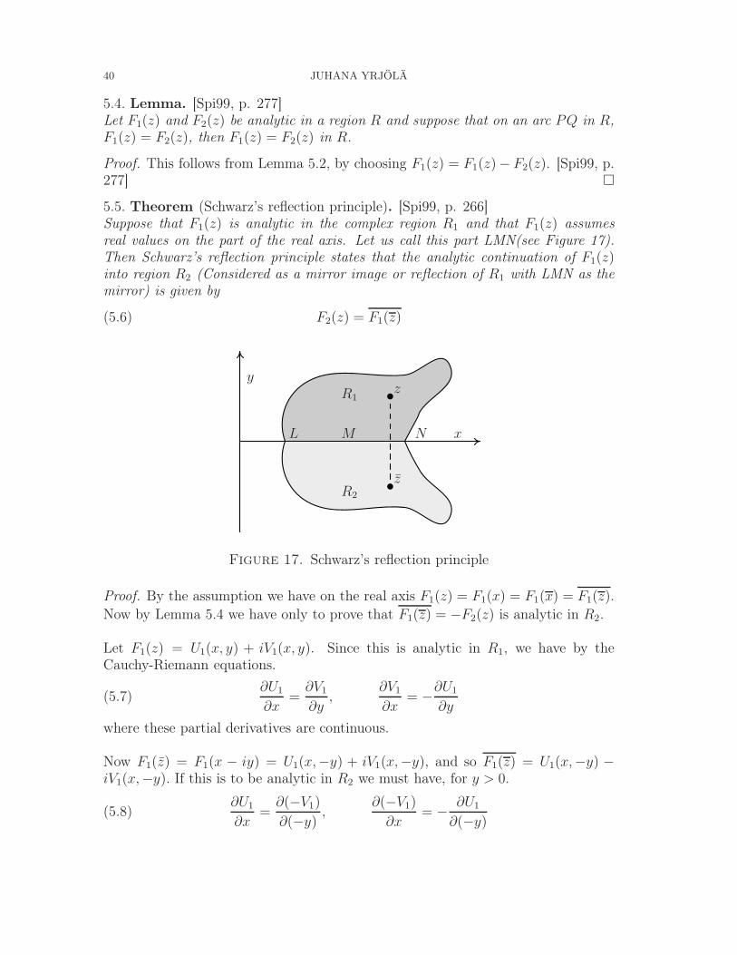
40 JUHANA YRJÖLÄ
5.4. Lemma. [Spi99, p. 277]Let F1(z) and F2(z) be analytic in a region R and suppose that on an arc PQ in R,F1(z) = F2(z), then F1(z) = F2(z) in R.
Proof. This follows from Lemma 5.2, by choosing F1(z) = F1(z)− F2(z). [Spi99, p.277]
5.5. Theorem (Schwarz’s reflection principle). [Spi99, p. 266]Suppose that F1(z) is analytic in the complex region R1 and that F1(z) assumesreal values on the part of the real axis. Let us call this part LMN(see Figure 17).Then Schwarz’s reflection principle states that the analytic continuation of F1(z)into region R2 (Considered as a mirror image or reflection of R1 with LMN as themirror) is given by
(5.6) F2(z) = F1(z)
L M N x
yR1
R2
z
z
Figure 17. Schwarz’s reflection principle
Proof. By the assumption we have on the real axis F1(z) = F1(x) = F1(x) = F1(z).
Now by Lemma 5.4 we have only to prove that F1(z) = −F2(z) is analytic in R2.
Let F1(z) = U1(x, y) + iV1(x, y). Since this is analytic in R1, we have by theCauchy-Riemann equations.
(5.7)∂U1
∂x=
∂V1
∂y,
∂V1
∂x= −∂U1
∂y
where these partial derivatives are continuous.
Now F1(z) = F1(x − iy) = U1(x,−y) + iV1(x,−y), and so F1(z) = U1(x,−y) −iV1(x,−y). If this is to be analytic in R2 we must have, for y > 0.
(5.8)∂U1
∂x=
∂(−V1)
∂(−y),
∂(−V1)
∂x= − ∂U1
∂(−y)
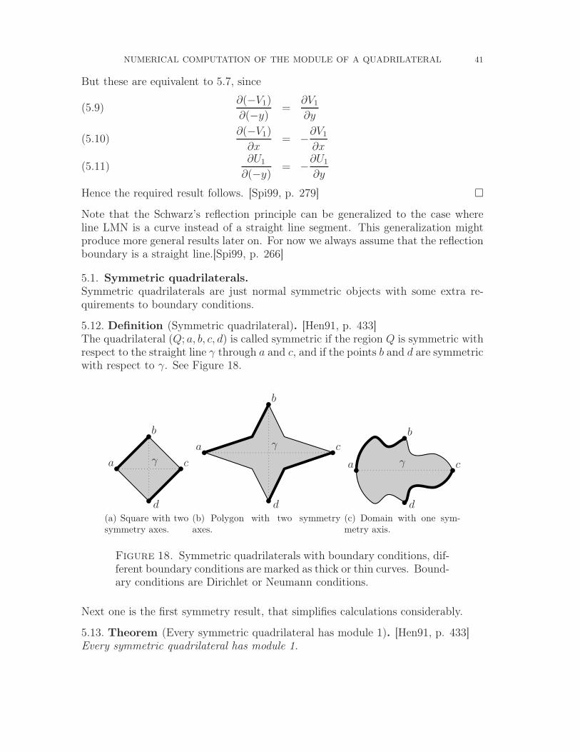
NUMERICAL COMPUTATION OF THE MODULE OF A QUADRILATERAL 41
But these are equivalent to 5.7, since
∂(−V1)
∂(−y)=
∂V1
∂y(5.9)
∂(−V1)
∂x= −∂V1
∂x(5.10)
∂U1
∂(−y)= −∂U1
∂y(5.11)
Hence the required result follows. [Spi99, p. 279]
Note that the Schwarz’s reflection principle can be generalized to the case whereline LMN is a curve instead of a straight line segment. This generalization mightproduce more general results later on. For now we always assume that the reflectionboundary is a straight line.[Spi99, p. 266]
5.1. Symmetric quadrilaterals.
Symmetric quadrilaterals are just normal symmetric objects with some extra re-quirements to boundary conditions.
5.12. Definition (Symmetric quadrilateral). [Hen91, p. 433]The quadrilateral (Q; a, b, c, d) is called symmetric if the region Q is symmetric withrespect to the straight line γ through a and c, and if the points b and d are symmetricwith respect to γ. See Figure 18.
a
b
c
d
γ
(a) Square with twosymmetry axes.
a
b
c
d
γ
(b) Polygon with two symmetryaxes.
a
b
c
d
γ
(c) Domain with one sym-metry axis.
Figure 18. Symmetric quadrilaterals with boundary conditions, dif-ferent boundary conditions are marked as thick or thin curves. Bound-ary conditions are Dirichlet or Neumann conditions.
Next one is the first symmetry result, that simplifies calculations considerably.
5.13. Theorem (Every symmetric quadrilateral has module 1). [Hen91, p. 433]Every symmetric quadrilateral has module 1.
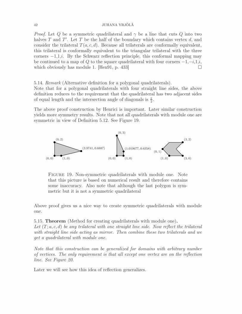
42 JUHANA YRJÖLÄ
Proof. Let Q be a symmetric quadrilateral and γ be a line that cuts Q into twohalves T and T ′. Let T be the half of the boundary which contains vertex d, andconsider the trilateral T (a, c, d). Because all trilaterals are conformally equivalent,this trilateral is conformally equivalent to the triangular trilateral with the threecorners −1,1,i. By the Schwarz reflection principle, this conformal mapping maybe continued to a map of Q to the square quadrilateral with four corners −1,−i,1,i,which obviously has module 1. [Hen91, p. 433]
5.14. Remark (Alternative definition for a polygonal quadrilaterals).Note that for a polygonal quadrilaterals with four straight line sides, the abovedefinition reduces to the requirement that the quadrilateral has two adjacent sidesof equal length and the intersection angle of diagonals is π
2.
The above proof construction by Henrici is important. Later similar constructionyields more symmetry results. Note that not all quadrilaterals with module one aresymmetric in view of Definition 5.12. See Figure 19.
(0, 0) (1, 0)
(3.9741, 0.6887)
(0, 2)
(0, 0) (1, 0)
(1.010677, 0.6358)
(0, 3)
(0, 1)
(1, 0) (3, 0)
(3, 2)
Figure 19. Non-symmetric quadrilaterals with module one. Notethat this picture is based on numerical result and therefore containssome inaccuracy. Also note that although the last polygon is sym-metric but it is not a symmetric quadrilateral
Above proof gives us a nice way to create symmetric quadrilaterals with moduleone.
5.15. Theorem (Method for creating quadrilaterals with module one).Let (T ; a, c, d) be any trilateral with one straight line side. Now reflect the trilateralwith straight line side acting as mirror. Then combine these two trilaterals and weget a quadrilateral with module one.
Note that this construction can be generalized for domains with arbitrary numberof vertices. The only requirement is that all except one vertex are on the reflectionline. See Figure 20.
Later we will see how this idea of reflection generalizes.
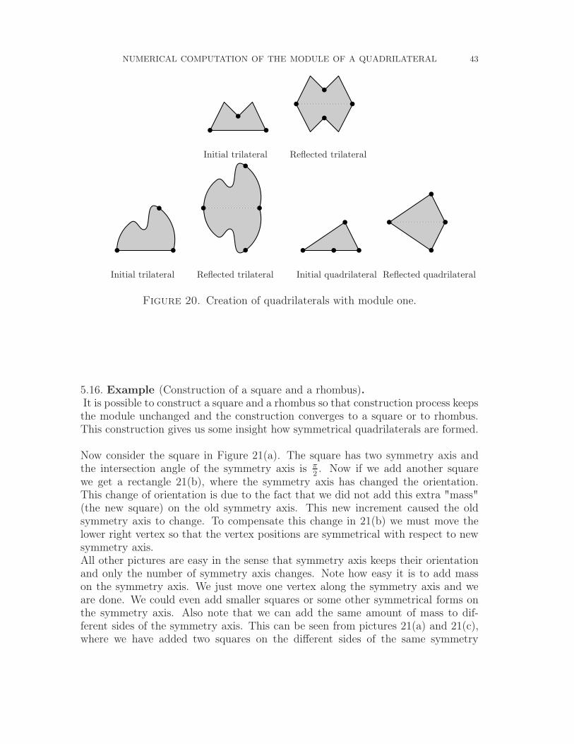
NUMERICAL COMPUTATION OF THE MODULE OF A QUADRILATERAL 43
Initial trilateral Reflected trilateral
Initial trilateral Reflected trilateral Initial quadrilateral Reflected quadrilateral
Figure 20. Creation of quadrilaterals with module one.
5.16. Example (Construction of a square and a rhombus).It is possible to construct a square and a rhombus so that construction process keepsthe module unchanged and the construction converges to a square or to rhombus.This construction gives us some insight how symmetrical quadrilaterals are formed.
Now consider the square in Figure 21(a). The square has two symmetry axis andthe intersection angle of the symmetry axis is π
2. Now if we add another square
we get a rectangle 21(b), where the symmetry axis has changed the orientation.This change of orientation is due to the fact that we did not add this extra "mass"(the new square) on the old symmetry axis. This new increment caused the oldsymmetry axis to change. To compensate this change in 21(b) we must move thelower right vertex so that the vertex positions are symmetrical with respect to newsymmetry axis.All other pictures are easy in the sense that symmetry axis keeps their orientationand only the number of symmetry axis changes. Note how easy it is to add masson the symmetry axis. We just move one vertex along the symmetry axis and weare done. We could even add smaller squares or some other symmetrical forms onthe symmetry axis. Also note that we can add the same amount of mass to dif-ferent sides of the symmetry axis. This can be seen from pictures 21(a) and 21(c),where we have added two squares on the different sides of the same symmetry
44 JUHANA YRJÖLÄ
axis symmetrically13. It should be emphasized that this works only for symmet-ric quadrilaterals, like those in Figure 21. Also note there is one picture missingfrom the construction given below. The picture is obviously square x4, which isjust a square. We can add multiple items at the same time too. For example wecould easily get from 21(d) to 21(h) by inserting four squares in the corners of 21(d).
For a rhombus this construction is similar, however apparently there does not existrhombus x2 object, that could be used in our construction easily. This is to beexpected since rhombus is more general form of the square. Note that this con-struction is also possible for kites and concave symmetric quadrilaterals but thenwe need to use at least two different kinds of building blocks.
13This construction might give a way to tile a square, when we use different block sizes. Ainteresting fact is that the connection between the square tilings and the conformal module havebeen studied previously by Cannon, Floyd and Parry, see [CFP96].
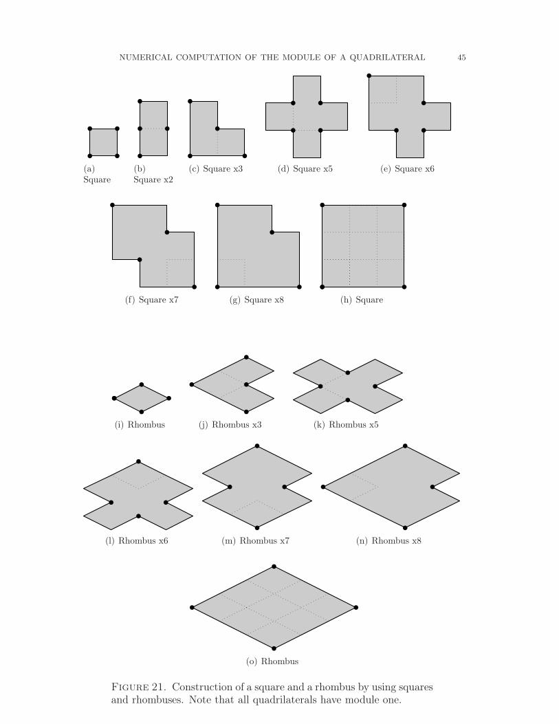
NUMERICAL COMPUTATION OF THE MODULE OF A QUADRILATERAL 45
(a)Square
(b)Square x2
(c) Square x3 (d) Square x5 (e) Square x6
(f) Square x7 (g) Square x8 (h) Square
(i) Rhombus (j) Rhombus x3 (k) Rhombus x5
(l) Rhombus x6 (m) Rhombus x7 (n) Rhombus x8
(o) Rhombus
Figure 21. Construction of a square and a rhombus by using squaresand rhombuses. Note that all quadrilaterals have module one.
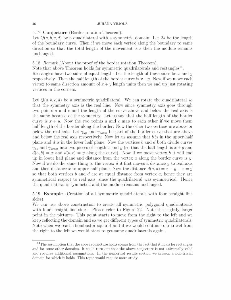
46 JUHANA YRJÖLÄ
5.17. Conjecture (Border rotation Theorem).Let Q(a, b, c, d) be a quadrilateral with a symmetric domain. Let 2s be the lengthof the boundary curve. Then if we move each vertex along the boundary to samedirection so that the total length of the movement is s then the module remainsunchanged.
5.18. Remark (About the proof of the border rotation Theorem).Note that above Theorem holds for symmetric quadrilaterals and rectangles14.Rectangles have two sides of equal length. Let the length of these sides be x and yrespectively. Then the half length of the border curve is x+y. Now if we move eachvertex to same direction amount of x + y length units then we end up just rotatingvertices in the corners.
Let Q(a, b, c, d) be a symmetric quadrilateral. We can rotate the quadrilateral sothat the symmetry axis is the real line. Now since symmetry axis goes throughtwo points a and c and the length of the curve above and below the real axis isthe same because of the symmetry. Let us say that the half length of the bordercurve is x + y. Now the two points a and c map to each other if we move themhalf length of the border along the border. Now the other two vertices are above orbelow the real axis. Let γup and γdown be part of the border curve that are aboveand below the real axis respectively. Now let us assume that b is in the upper halfplane and d is in the lower half plane. Now the vertices b and d both divide curvesγup and γdown into two pieces of length x and y (so that the half length is x + y andd(a, b) = x and d(b, c) = y along the curve). Now if we move vertex b it will endup in lower half plane and distance from the vertex a along the border curve is y.Now if we do the same thing to the vertex d it first moves a distance y to real axisand then distance x to upper half plane. Now the distance d(a, d) = x + y − x = yso that both vertices b and d are at equal distance from vertex a, hence they aresymmetrical respect to real axis, since the quadrilateral was symmetrical. Hencethe quadrilateral is symmetric and the module remains unchanged.
5.19. Example (Creation of all symmetric quadrilaterals with four straight linesides).We can use above construction to create all symmetric polygonal quadrilateralswith four straight line sides. Please refer to Figure 22. Note the slightly largerpoint in the pictures. This point starts to move from the right to the left and wekeep reflecting the domain and so we get different types of symmetric quadrilaterals.Note when we reach rhombus(or square) and if we would continue our travel fromthe right to the left we would start to get same quadrilaterals again.
14The assumption that the above conjecture holds comes from the fact that it holds for rectanglesand for some other domains. It could turn out that the above conjecture is not universally validand requires additional assumptions. In the numerical results section we present a non-trivialdomain for which it holds. This topic would require more study.
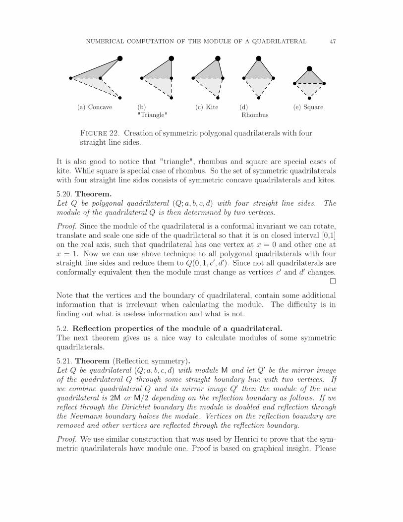
NUMERICAL COMPUTATION OF THE MODULE OF A QUADRILATERAL 47
(a) Concave (b)"Triangle"
(c) Kite (d)Rhombus
(e) Square
Figure 22. Creation of symmetric polygonal quadrilaterals with fourstraight line sides.
It is also good to notice that "triangle", rhombus and square are special cases ofkite. While square is special case of rhombus. So the set of symmetric quadrilateralswith four straight line sides consists of symmetric concave quadrilaterals and kites.
5.20. Theorem.
Let Q be polygonal quadrilateral (Q; a, b, c, d) with four straight line sides. Themodule of the quadrilateral Q is then determined by two vertices.
Proof. Since the module of the quadrilateral is a conformal invariant we can rotate,translate and scale one side of the quadrilateral so that it is on closed interval [0,1]on the real axis, such that quadrilateral has one vertex at x = 0 and other one atx = 1. Now we can use above technique to all polygonal quadrilaterals with fourstraight line sides and reduce them to Q(0, 1, c′, d′). Since not all quadrilaterals areconformally equivalent then the module must change as vertices c′ and d′ changes.
Note that the vertices and the boundary of quadrilateral, contain some additionalinformation that is irrelevant when calculating the module. The difficulty is infinding out what is useless information and what is not.
5.2. Reflection properties of the module of a quadrilateral.
The next theorem gives us a nice way to calculate modules of some symmetricquadrilaterals.
5.21. Theorem (Reflection symmetry).Let Q be quadrilateral (Q; a, b, c, d) with module M and let Q′ be the mirror imageof the quadrilateral Q through some straight boundary line with two vertices. Ifwe combine quadrilateral Q and its mirror image Q′ then the module of the newquadrilateral is 2M or M/2 depending on the reflection boundary as follows. If wereflect through the Dirichlet boundary the module is doubled and reflection throughthe Neumann boundary halves the module. Vertices on the reflection boundary areremoved and other vertices are reflected through the reflection boundary.
Proof. We use similar construction that was used by Henrici to prove that the sym-metric quadrilaterals have module one. Proof is based on graphical insight. Please
48 JUHANA YRJÖLÄ
see Figure 23.
Let Q = (Q; a, b, c, d) be the quadrilateral to be reflected, as above. Now by as-sumption quadrilateral Q has one straight line as its boundary curve. We can placethis boundary line on the x-axis by a simple conformal rotation. Since quadrilateralQ has module M we can map the quadrilateral Q conformally to rectangle with sidelengths 1 and M respectively. Now by the Schwarz reflection principle we can extendthis map to its mirror image too. We get a map from domain Q ∪ Q′ to rectanglewith side lengths 1 and 2M or 2 and M. The side lengths depend on the reflectionboundary as follows.
• Reflection boundary is the Neumann boundary.If the reflection boundary is the Neumann boundary, then we must orient ourrectangle in the same way because of the Schwarz reflection principle requiresthat on the reflection boundary both functions must take same values. Fora rectangle this means that the side lengths of the rectangle are 2 and M.Now if we calculate the module of the rectangle by formula (3.49) we haveM/2.
• Reflection boundary is the Dirichlet boundary.If the reflection boundary is the Dirichlet boundary, then we must againorient our rectangle in same way as above. This time, however, the sidelengths of the rectangle are 1 and 2M. Now if we calculate the module ofthis rectangle by (3.49) we get 2M.
Since Q ∪ Q′ and rectangle are conformally equivalent we can conclude that themodule of the quadrilateral Q∪Q′ is 2M or M/2 depending on the reflection bound-ary.
Note that our form of Schwarz’s reflection principle requires that the reflectionboundary is a straight line. Proof might be generalized to case where reflectionboundary is some kind of a curve. Also note that if we do two reflections one throughthe Dirichlet boundary and other one through the Neumann boundary(or other wayaround) then the module of the resulting quadrilateral remains unchanged.
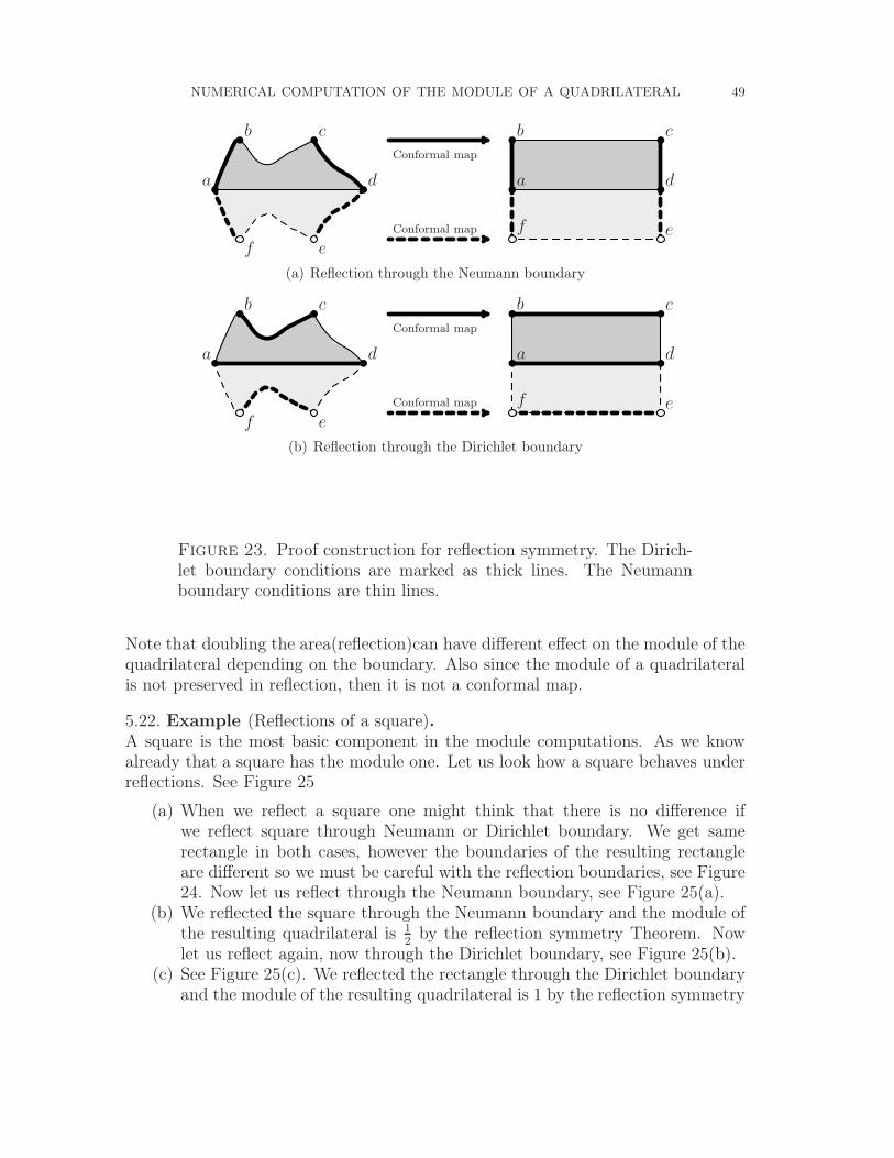
NUMERICAL COMPUTATION OF THE MODULE OF A QUADRILATERAL 49
a
b c
d
ef
Conformal map
Conformal map
a
b c
d
ef
(a) Reflection through the Neumann boundary
a
b c
d
ef
Conformal map
Conformal map
a
b c
d
ef
(b) Reflection through the Dirichlet boundary
Figure 23. Proof construction for reflection symmetry. The Dirich-let boundary conditions are marked as thick lines. The Neumannboundary conditions are thin lines.
Note that doubling the area(reflection)can have different effect on the module of thequadrilateral depending on the boundary. Also since the module of a quadrilateralis not preserved in reflection, then it is not a conformal map.
5.22. Example (Reflections of a square).A square is the most basic component in the module computations. As we knowalready that a square has the module one. Let us look how a square behaves underreflections. See Figure 25
(a) When we reflect a square one might think that there is no difference ifwe reflect square through Neumann or Dirichlet boundary. We get samerectangle in both cases, however the boundaries of the resulting rectangleare different so we must be careful with the reflection boundaries, see Figure24. Now let us reflect through the Neumann boundary, see Figure 25(a).
(b) We reflected the square through the Neumann boundary and the module ofthe resulting quadrilateral is 1
2by the reflection symmetry Theorem. Now
let us reflect again, now through the Dirichlet boundary, see Figure 25(b).(c) See Figure 25(c). We reflected the rectangle through the Dirichlet boundary
and the module of the resulting quadrilateral is 1 by the reflection symmetry
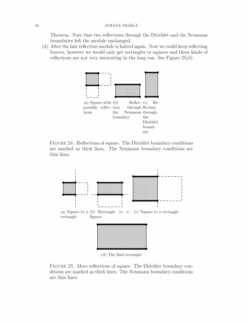
50 JUHANA YRJÖLÄ
Theorem. Note that two reflections through the Dirichlet and the Neumannboundaries left the module unchanged.
(d) After the last reflection module is halved again. Now we could keep reflectingforever, however we would only get rectangles or squares and these kinds ofreflections are not very interesting in the long run. See Figure 25(d).
(a) Square withpossible reflec-tions
(b) Reflec-tion throughthe Neumannboundary
(c) Re-flectionthroughtheDirichletbound-ary
Figure 24. Reflections of square. The Dirichlet boundary conditionsare marked as thick lines. The Neumann boundary conditions arethin lines.
(a) Square to arectangle
(b) Rectangle to aSquare
(c) Square to a rectangle
(d) The final rectangle
Figure 25. More reflections of square. The Dirichlet boundary con-ditions are marked as thick lines. The Neumann boundary conditionsare thin lines.
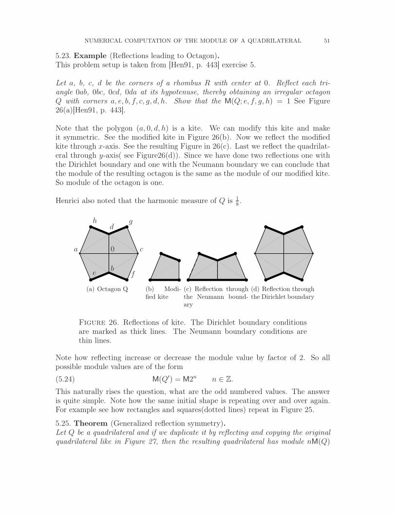
NUMERICAL COMPUTATION OF THE MODULE OF A QUADRILATERAL 51
5.23. Example (Reflections leading to Octagon).This problem setup is taken from [Hen91, p. 443] exercise 5.
Let a, b, c, d be the corners of a rhombus R with center at 0. Reflect each tri-angle 0ab, 0bc, 0cd, 0da at its hypotenuse, thereby obtaining an irregular octagonQ with corners a, e, b, f, c, g, d, h. Show that the M(Q; e, f, g, h) = 1 See Figure26(a)[Hen91, p. 443].
Note that the polygon (a, 0, d, h) is a kite. We can modify this kite and makeit symmetric. See the modified kite in Figure 26(b). Now we reflect the modifiedkite through x-axis. See the resulting Figure in 26(c). Last we reflect the quadrilat-eral through y-axis( see Figure26(d)). Since we have done two reflections one withthe Dirichlet boundary and one with the Neumann boundary we can conclude thatthe module of the resulting octagon is the same as the module of our modified kite.So module of the octagon is one.
Henrici also noted that the harmonic measure of Q is 18.
a
b
c
d
e f
gh
0
(a) Octagon Q (b) Modi-fied kite
(c) Reflection throughthe Neumann bound-ary
(d) Reflection throughthe Dirichlet boundary
Figure 26. Reflections of kite. The Dirichlet boundary conditionsare marked as thick lines. The Neumann boundary conditions arethin lines.
Note how reflecting increase or decrease the module value by factor of 2. So allpossible module values are of the form
(5.24) M(Q′) = M2n n ∈ Z.
This naturally rises the question, what are the odd numbered values. The answeris quite simple. Note how the same initial shape is repeating over and over again.For example see how rectangles and squares(dotted lines) repeat in Figure 25.
5.25. Theorem (Generalized reflection symmetry).Let Q be a quadrilateral and if we duplicate it by reflecting and copying the originalquadrilateral like in Figure 27, then the resulting quadrilateral has module nM(Q)
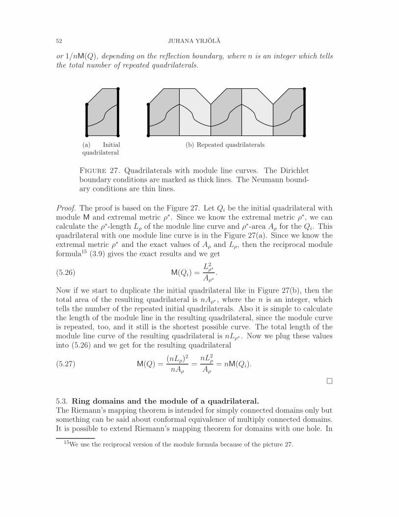
52 JUHANA YRJÖLÄ
or 1/nM(Q), depending on the reflection boundary, where n is an integer which tellsthe total number of repeated quadrilaterals.
(a) Initialquadrilateral
(b) Repeated quadrilaterals
Figure 27. Quadrilaterals with module line curves. The Dirichletboundary conditions are marked as thick lines. The Neumann bound-ary conditions are thin lines.
Proof. The proof is based on the Figure 27. Let Qi be the initial quadrilateral withmodule M and extremal metric ρ∗. Since we know the extremal metric ρ∗, we cancalculate the ρ∗-length Lρ of the module line curve and ρ∗-area Aρ for the Qi. Thisquadrilateral with one module line curve is in the Figure 27(a). Since we know theextremal metric ρ∗ and the exact values of Aρ and Lρ, then the reciprocal moduleformula15 (3.9) gives the exact results and we get
(5.26) M(Qi) =L2
ρ∗
Aρ∗.
Now if we start to duplicate the initial quadrilateral like in Figure 27(b), then thetotal area of the resulting quadrilateral is nAρ∗ , where the n is an integer, whichtells the number of the repeated initial quadrilaterals. Also it is simple to calculatethe length of the module line in the resulting quadrilateral, since the module curveis repeated, too, and it still is the shortest possible curve. The total length of themodule line curve of the resulting quadrilateral is nLρ∗ . Now we plug these valuesinto (5.26) and we get for the resulting quadrilateral
(5.27) M(Q) =(nLρ)
2
nAρ
=nL2
ρ
Aρ
= nM(Qi).
5.3. Ring domains and the module of a quadrilateral.
The Riemann’s mapping theorem is intended for simply connected domains only butsomething can be said about conformal equivalence of multiply connected domains.It is possible to extend Riemann’s mapping theorem for domains with one hole. In
15We use the reciprocal version of the module formula because of the picture 27.
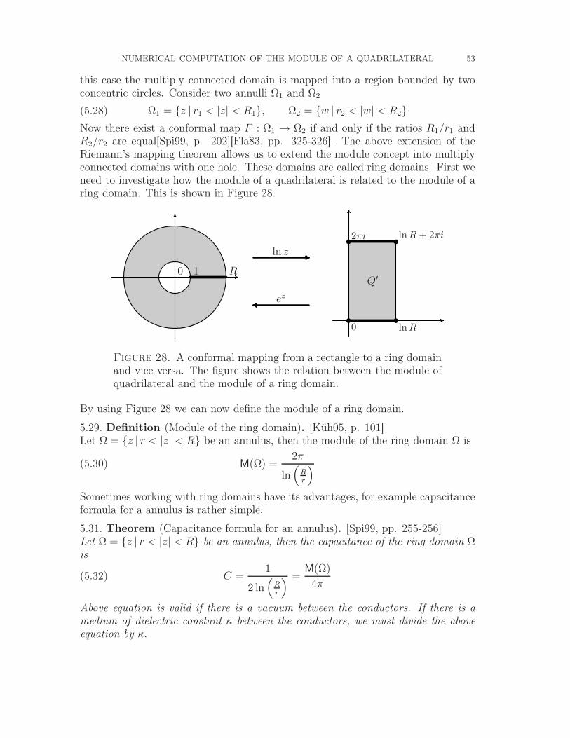
NUMERICAL COMPUTATION OF THE MODULE OF A QUADRILATERAL 53
this case the multiply connected domain is mapped into a region bounded by twoconcentric circles. Consider two annulli Ω1 and Ω2
(5.28) Ω1 = z | r1 < |z| < R1, Ω2 = w | r2 < |w| < R2Now there exist a conformal map F : Ω1 → Ω2 if and only if the ratios R1/r1 andR2/r2 are equal[Spi99, p. 202][Fla83, pp. 325-326]. The above extension of theRiemann’s mapping theorem allows us to extend the module concept into multiplyconnected domains with one hole. These domains are called ring domains. First weneed to investigate how the module of a quadrilateral is related to the module of aring domain. This is shown in Figure 28.
0 1 R
ln z
ez
0 ln R
ln R + 2πi2πi
Q′
Figure 28. A conformal mapping from a rectangle to a ring domainand vice versa. The figure shows the relation between the module ofquadrilateral and the module of a ring domain.
By using Figure 28 we can now define the module of a ring domain.
5.29. Definition (Module of the ring domain). [Küh05, p. 101]Let Ω = z | r < |z| < R be an annulus, then the module of the ring domain Ω is
(5.30) M(Ω) =2π
ln(
Rr
)
Sometimes working with ring domains have its advantages, for example capacitanceformula for a annulus is rather simple.
5.31. Theorem (Capacitance formula for an annulus). [Spi99, pp. 255-256]Let Ω = z | r < |z| < R be an annulus, then the capacitance of the ring domain Ωis
(5.32) C =1
2 ln(
Rr
) =M(Ω)
4π
Above equation is valid if there is a vacuum between the conductors. If there is amedium of dielectric constant κ between the conductors, we must divide the aboveequation by κ.
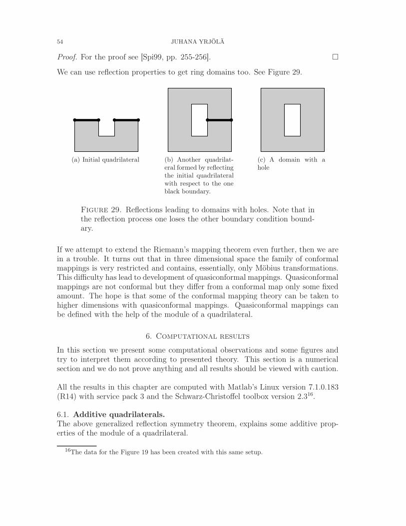
54 JUHANA YRJÖLÄ
Proof. For the proof see [Spi99, pp. 255-256].
We can use reflection properties to get ring domains too. See Figure 29.
(a) Initial quadrilateral (b) Another quadrilat-eral formed by reflectingthe initial quadrilateralwith respect to the oneblack boundary.
(c) A domain with ahole
Figure 29. Reflections leading to domains with holes. Note that inthe reflection process one loses the other boundary condition bound-ary.
If we attempt to extend the Riemann’s mapping theorem even further, then we arein a trouble. It turns out that in three dimensional space the family of conformalmappings is very restricted and contains, essentially, only Möbius transformations.This difficulty has lead to development of quasiconformal mappings. Quasiconformalmappings are not conformal but they differ from a conformal map only some fixedamount. The hope is that some of the conformal mapping theory can be taken tohigher dimensions with quasiconformal mappings. Quasiconformal mappings canbe defined with the help of the module of a quadrilateral.
6. Computational results
In this section we present some computational observations and some figures andtry to interpret them according to presented theory. This section is a numericalsection and we do not prove anything and all results should be viewed with caution.
All the results in this chapter are computed with Matlab’s Linux version 7.1.0.183(R14) with service pack 3 and the Schwarz-Christoffel toolbox version 2.316.
6.1. Additive quadrilaterals.
The above generalized reflection symmetry theorem, explains some additive prop-erties of the module of a quadrilateral.
16The data for the Figure 19 has been created with this same setup.
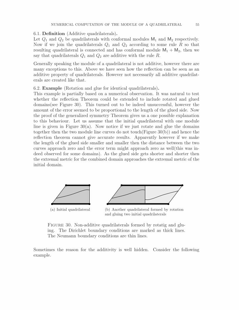
NUMERICAL COMPUTATION OF THE MODULE OF A QUADRILATERAL 55
6.1. Definition (Additive quadrilaterals).Let Q1 and Q2 be quadrilaterals with conformal modules M1 and M2 respectively.Now if we join the quadrilaterals Q1 and Q2 according to some rule R so thatresulting quadrilateral is connected and has conformal module M1 + M2, then wesay that quadrilaterals Q1 and Q2 are additive with the rule R.
Generally speaking the module of a quadrilateral is not additive, however there aremany exceptions to this. Above we have seen how the reflection can be seen as anadditive property of quadrilaterals. However not necessarily all additive quadrilat-erals are created like that.
6.2. Example (Rotation and glue for identical quadrilaterals).This example is partially based on a numerical observation. It was natural to testwhether the reflection Theorem could be extended to include rotated and glueddomains(see Figure 30). This turned out to be indeed unsuccessful, however theamount of the error seemed to be proportional to the length of the glued side. Nowthe proof of the generalized symmetry Theorem gives us a one possible explanationto this behaviour. Let us assume that the initial quadrilateral with one moduleline is given in Figure 30(a). Now notice if we just rotate and glue the domainstogether then the two module line curves do not touch(Figure 30(b)) and hence thereflection theorem cannot give accurate results. Apparently however if we makethe length of the glued side smaller and smaller then the distance between the twocurves approach zero and the error term might approach zero as well(this was in-deed observed for some domains). As the glued side gets shorter and shorter thenthe extremal metric for the combined domain approaches the extremal metric of theinitial domain.
(a) Initial quadrilateral (b) Another quadrilateral formed by rotationand gluing two initial quadrilaterals
Figure 30. Non-additive quadrilaterals formed by rotatig and glu-ing. The Dirichlet boundary conditions are marked as thick lines.The Neumann boundary conditions are thin lines.
Sometimes the reason for the additivity is well hidden. Consider the followingexample.
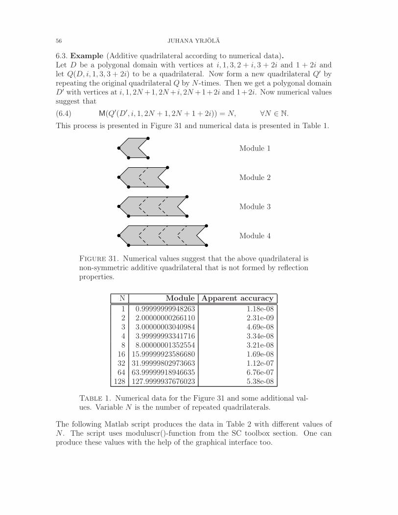
56 JUHANA YRJÖLÄ
6.3. Example (Additive quadrilateral according to numerical data).Let D be a polygonal domain with vertices at i, 1, 3, 2 + i, 3 + 2i and 1 + 2i andlet Q(D, i, 1, 3, 3 + 2i) to be a quadrilateral. Now form a new quadrilateral Q′ byrepeating the original quadrilateral Q by N -times. Then we get a polygonal domainD′ with vertices at i, 1, 2N +1, 2N + i, 2N +1+2i and 1+2i. Now numerical valuessuggest that
(6.4) M(Q′(D′, i, 1, 2N + 1, 2N + 1 + 2i)) = N, ∀N ∈ N.
This process is presented in Figure 31 and numerical data is presented in Table 1.
Module 1
Module 2
Module 3
Module 4
Figure 31. Numerical values suggest that the above quadrilateral isnon-symmetric additive quadrilateral that is not formed by reflectionproperties.
N Module Apparent accuracy
1 0.99999999948263 1.18e-082 2.00000000266110 2.31e-093 3.00000003040984 4.69e-084 3.99999993341716 3.34e-088 8.00000001352554 3.21e-08
16 15.99999923586680 1.69e-0832 31.99999802973663 1.12e-0764 63.99999918946635 6.76e-07
128 127.9999937676023 5.38e-08
Table 1. Numerical data for the Figure 31 and some additional val-ues. Variable N is the number of repeated quadrilaterals.
The following Matlab script produces the data in Table 2 with different values ofN . The script uses moduluscr()-function from the SC toolbox section. One canproduce these values with the help of the graphical interface too.
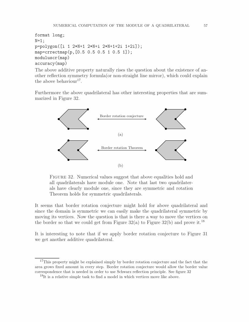
NUMERICAL COMPUTATION OF THE MODULE OF A QUADRILATERAL 57
format long;
N=1;
p=polygon([i 1 2*N+1 2*N+i 2*N+1+2i 1+2i]);
map=crrectmap(p,[0.5 0.5 0.5 1 0.5 1]);
moduluscr(map)
accuracy(map)
The above additive property naturally rises the question about the existence of an-other reflection symmetry formula(or non-straight line mirror), which could explainthe above behaviour17.
Furthermore the above quadrilateral has other interesting properties that are sum-marized in Figure 32.
Border rotation conjecture
(a)
Border rotation Theorem
(b)
Figure 32. Numerical values suggest that above equalities hold andall quadrilaterals have module one. Note that last two quadrilater-als have clearly module one, since they are symmetric and rotationTheorem holds for symmetric quadrilaterals.
It seems that border rotation conjecture might hold for above quadrilateral andsince the domain is symmetric we can easily make the quadrilateral symmetric bymoving its vertices. Now the question is that is there a way to move the vertices onthe border so that we could get from Figure 32(a) to Figure 32(b) and prove it.18
It is interesting to note that if we apply border rotation conjecture to Figure 31we get another additive quadrilateral.
17This property might be explained simply by border rotation conjecture and the fact that thearea grows fixed amount in every step. Border rotation conjecture would allow the border valuecorrespondence that is needed in order to use Schwarz reflection principle. See figure 32
18It is a relative simple task to find a model in which vertices move like above.
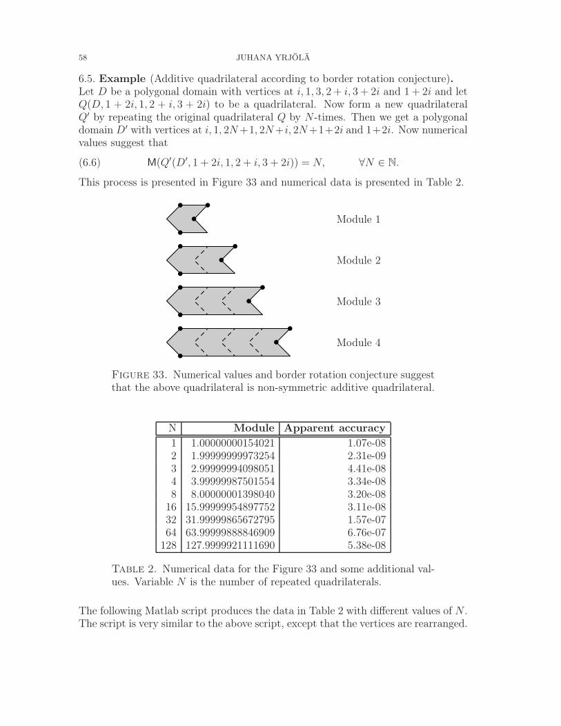
58 JUHANA YRJÖLÄ
6.5. Example (Additive quadrilateral according to border rotation conjecture).Let D be a polygonal domain with vertices at i, 1, 3, 2 + i, 3 + 2i and 1 + 2i and letQ(D, 1 + 2i, 1, 2 + i, 3 + 2i) to be a quadrilateral. Now form a new quadrilateralQ′ by repeating the original quadrilateral Q by N -times. Then we get a polygonaldomain D′ with vertices at i, 1, 2N +1, 2N +i, 2N +1+2i and 1+2i. Now numericalvalues suggest that
(6.6) M(Q′(D′, 1 + 2i, 1, 2 + i, 3 + 2i)) = N, ∀N ∈ N.
This process is presented in Figure 33 and numerical data is presented in Table 2.
Module 1
Module 2
Module 3
Module 4
Figure 33. Numerical values and border rotation conjecture suggestthat the above quadrilateral is non-symmetric additive quadrilateral.
N Module Apparent accuracy
1 1.00000000154021 1.07e-082 1.99999999973254 2.31e-093 2.99999994098051 4.41e-084 3.99999987501554 3.34e-088 8.00000001398040 3.20e-08
16 15.99999954897752 3.11e-0832 31.99999865672795 1.57e-0764 63.99999888846909 6.76e-07
128 127.9999921111690 5.38e-08
Table 2. Numerical data for the Figure 33 and some additional val-ues. Variable N is the number of repeated quadrilaterals.
The following Matlab script produces the data in Table 2 with different values of N .The script is very similar to the above script, except that the vertices are rearranged.
NUMERICAL COMPUTATION OF THE MODULE OF A QUADRILATERAL 59
format long;
N=1;
p=polygon([1+2i i 1 2*N+1 2*N+i 2*N+1+2i]);
map=crrectmap(p,[0.5 1 0.5 1 0.5 0.5]);
moduluscr(map)
accuracy(map)
6.2. The module of a quadrilateral under movement of one vertex.
Next we investigate what happens to the module of a quadrilateral if one of its vertexstarts to move, while other vertices remain still19. The Matlab source code for thecreation of the numerical data and ploting script for the data is available in theappendix. All the data was created by the following function call with parametersgiven below, where n ∈ 0.5 1 2 3 4 520.
imagematrix=computeData(151,8,n);
Consider the situation in Figure 34. The original quadrilateral is displayed as a bluerectangle. Vertices on the axis remain still, while the remaining vertex moves tosome point P . The background color at point P shows the module of the quadrilat-eral with moving vertex at point P . Also since the background color is somewhathard to interpret we have added some contour lines. These contour lines show pathsfor which module remains unchanged under the movement of one vertex. The valueof the constant module is displayed on the contour line.
It is interesting to note that in Figure 34(b) module of the quadrilateral gets recip-rocal values on the different sides of the symmetry axis y = x(for example see lines1.11 and 0.9, 1
1.11≈ 0.9). This is to be expected, since the resulting quadrilater-
als have the same domain and reciprocal boundary conditions. Next we list somegeneral observations from Figure 34.
• Note how the module is continuous in the sense that the constant modulecurve for the module of the original rectangle begins at the corner of theevery rectangle.
• Note that as we travel further and further away from the original rectanglewe need to make bigger changes in the position of the moving vertex to getthe same effect as moving near the original rectangle.
• Note that the constant module lines are curved to up or down, dependingon the position of the curve and the original quadrilateral. What makesthis even more interesting is the fact that apparently there always exist acurve which has a zero curvature(a line). In Figure 34(b) this curve withzero curvature is the symmetry axis. The zero curvature line in general has
19The module of a quadrilateral under the movement of one vertex have been studied before byDubinin and Vuorinen in [DV05].
20Total 23104 Schwarz-Christoffel transformations were calculated for each data set(differentvalues of n) and hence for each picture. This process took about 2-4h on a standard sharedworkstation.
60 JUHANA YRJÖLÄ
interesting properties. Consider Example 5.16, where it was relatively simpleto increase mass on the symmetry axis and move the vertex along the axis.This rises a question that could the zero curvature line be considered as ageneralized symmetry axis? This generalized symmetry axis would not needto be symmetric since it needs to grow in a unbalanced way to keep moduledifferent from 1. Also note that if the height of the rectangle is less than 1,then the zero curvature line is above the line y = x. On the other hand ifthe height of the rectangle is greater than 1 then the zero curvature line isbelow the line y = x. For example compare figures 34(a) and 34(c).
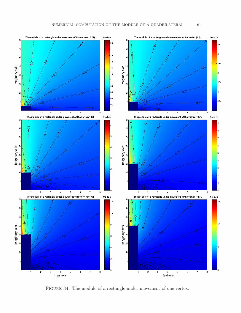
NUMERICAL COMPUTATION OF THE MODULE OF A QUADRILATERAL 61
Figure 34. The module of a rectangle under movement of one vertex.
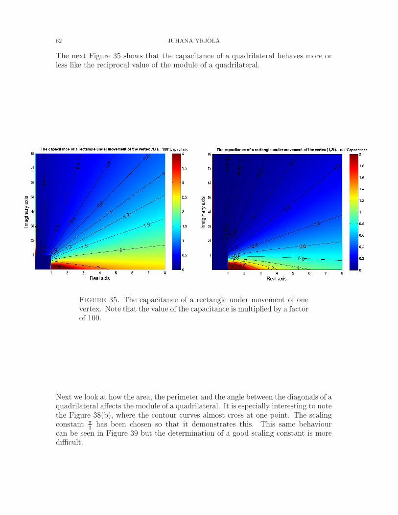
62 JUHANA YRJÖLÄ
The next Figure 35 shows that the capacitance of a quadrilateral behaves more orless like the reciprocal value of the module of a quadrilateral.
Figure 35. The capacitance of a rectangle under movement of onevertex. Note that the value of the capacitance is multiplied by a factorof 100.
Next we look at how the area, the perimeter and the angle between the diagonals of aquadrilateral affects the module of a quadrilateral. It is especially interesting to notethe Figure 38(b), where the contour curves almost cross at one point. The scalingconstant π
2has been chosen so that it demonstrates this. This same behaviour
can be seen in Figure 39 but the determination of a good scaling constant is moredifficult.
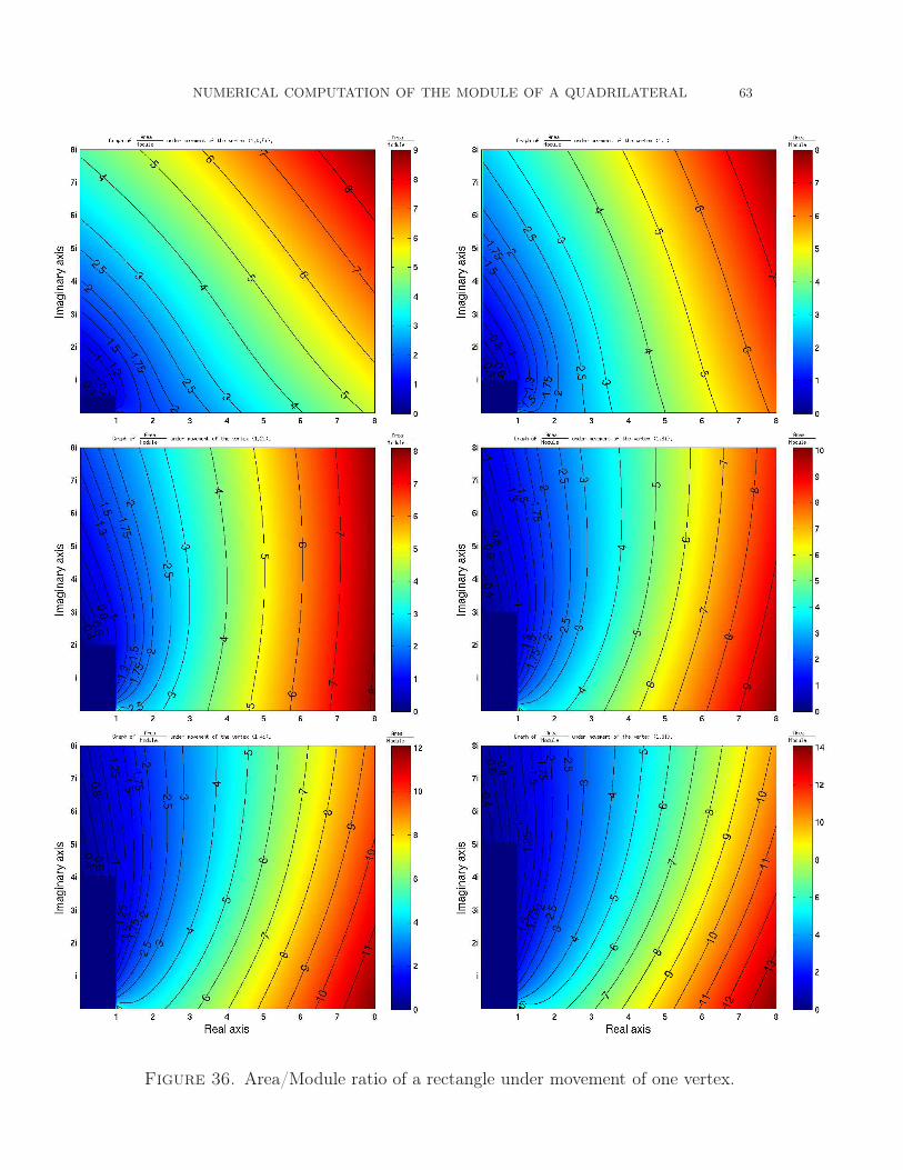
NUMERICAL COMPUTATION OF THE MODULE OF A QUADRILATERAL 63
Figure 36. Area/Module ratio of a rectangle under movement of one vertex.
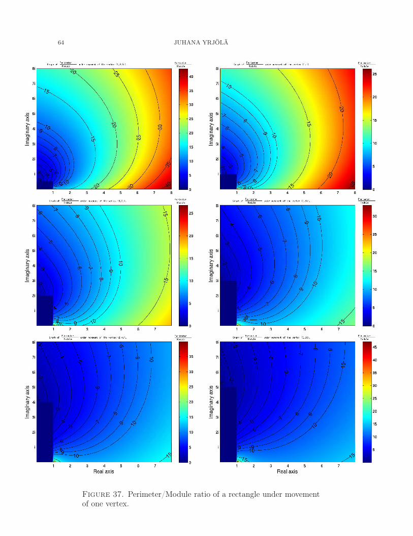
64 JUHANA YRJÖLÄ
Figure 37. Perimeter/Module ratio of a rectangle under movementof one vertex.
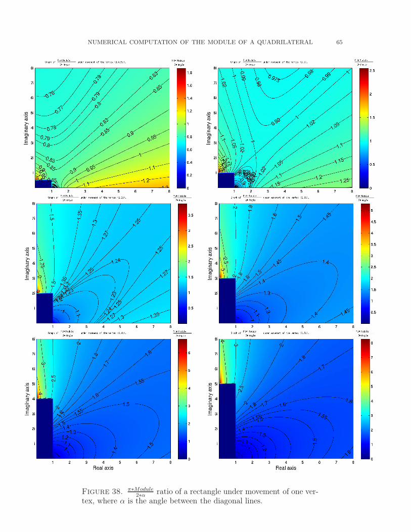
NUMERICAL COMPUTATION OF THE MODULE OF A QUADRILATERAL 65
Figure 38. π∗Module2∗α
ratio of a rectangle under movement of one ver-tex, where α is the angle between the diagonal lines.
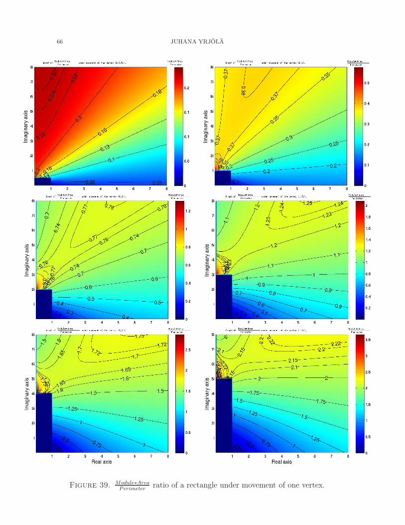
66 JUHANA YRJÖLÄ
Figure 39. Module∗AreaPerimeter
ratio of a rectangle under movement of one vertex.
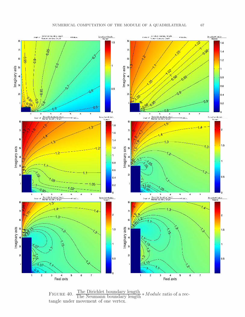
NUMERICAL COMPUTATION OF THE MODULE OF A QUADRILATERAL 67
Figure 40.The Dirichlet boundary lengthThe Neumann boundary length
∗Module ratio of a rec-
tangle under movement of one vertex.
68 JUHANA YRJÖLÄ
7. Other numerical methods
Numerical methods for the computation of the module of a quadrilateral are gen-erally very difficult to implement. Programs often need special functions and othercomputational tools. This tends to increase program size and programmer’s work-load, since only small amount of these tools/functions are found ready in languagespecific libraries. In addition to implementation difficulties, the needed backgroundmathematics are sometimes difficult. What makes this even worse is the fact thatsome methods are so badly documented, in scientific papers, that is very hard fora novice to even reproduce the same results. Therefore I have come to a conclu-sion that if someone actually publishes a new numerical algorithm it might be agood idea to publish well documented source code for that algorithm as well. Thiswould increase the probability that someone is actually going to use the algorithmand thus increase knowledge of the algorithm. Another advantage would be that itwould allow a writer to omit certain boring details from the scientific paper, whilethe person who is only interested in using the results would be able to do so. Nowa-days this would be very simple to do thanks to the Internet.
In this section we look at some simple methods for the computation of the module ofa quadrilateral and then move to more advanced stuff, for more conformal mappingtechniques see [Por06] 21 and [Küh05].
7.1. Challis & Burley iteration.
One of the easiest methods to implement is the Challis & Burley iteration. This it-eration was presented by N.V Challis and D.M Burley in 1981[CB82] and it is basedon discrete Fourier transformation. This method was then studied by D. Gaier andN. Papamichael and they showed that Challis & Burley iteration was a special caseof the method of Garrick[GP87]. They also provided convergence results and madesome practical observations. Simplicity of the Challis & Burley iteration comes witha price and the price is that the iteration domains are very restricted and conver-gence is usually bad.
The basic Challis & Burley iteration works only for quadrilaterals with followingdomains
(7.1) G = (x, y) : 0 < x < 1, 0 < y < f(x).where f(x) is arbitrary simple curve[CB82]. We call above domains as Challis &Burley domains22. Note that since we are only interested in computing the moduleof the quadrilateral we can extend the Challis & Burley domain to include anotherdomain which is formed by reflection.
21Antti Rasila has used the Koebe’s method, which is introduced in Porter’s paper but accordingto Rasila convergence is slow.
22Gaier and Papamichael showed that more general Garrick algorithm can be applied to moregeneral domains of the form G = (x, y) : 0 < x < 1, f1(x) < y < f2(x). [GP87]
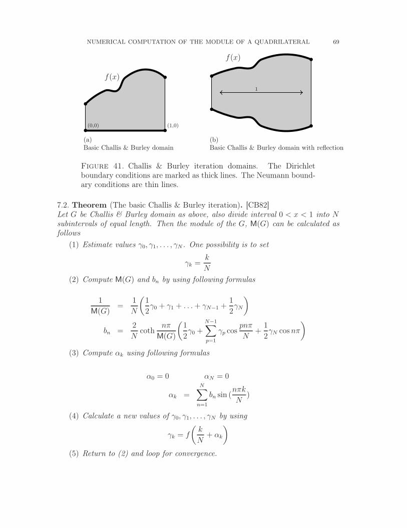
NUMERICAL COMPUTATION OF THE MODULE OF A QUADRILATERAL 69
(0,0) (1,0)
f(x)
(a)Basic Challis & Burley domain
1
f(x)
(b)Basic Challis & Burley domain with reflection
Figure 41. Challis & Burley iteration domains. The Dirichletboundary conditions are marked as thick lines. The Neumann bound-ary conditions are thin lines.
7.2. Theorem (The basic Challis & Burley iteration). [CB82]Let G be Challis & Burley domain as above, also divide interval 0 < x < 1 into Nsubintervals of equal length. Then the module of the G, M(G) can be calculated asfollows
(1) Estimate values γ0, γ1, . . . , γN . One possibility is to set
γk =k
N
(2) Compute M(G) and bn by using following formulas
1
M(G)=
1
N
(
1
2γ0 + γ1 + . . . + γN−1 +
1
2γN
)
bn =2
Ncoth
nπ
M(G)
(
1
2γ0 +
N−1∑
p=1
γp cospnπ
N+
1
2γN cos nπ
)
(3) Compute αk using following formulas
α0 = 0 αN = 0
αk =
N∑
n=1
bn sin (nπk
N)
(4) Calculate a new values of γ0, γ1, . . . , γN by using
γk = f
(
k
N+ αk
)
(5) Return to (2) and loop for convergence.
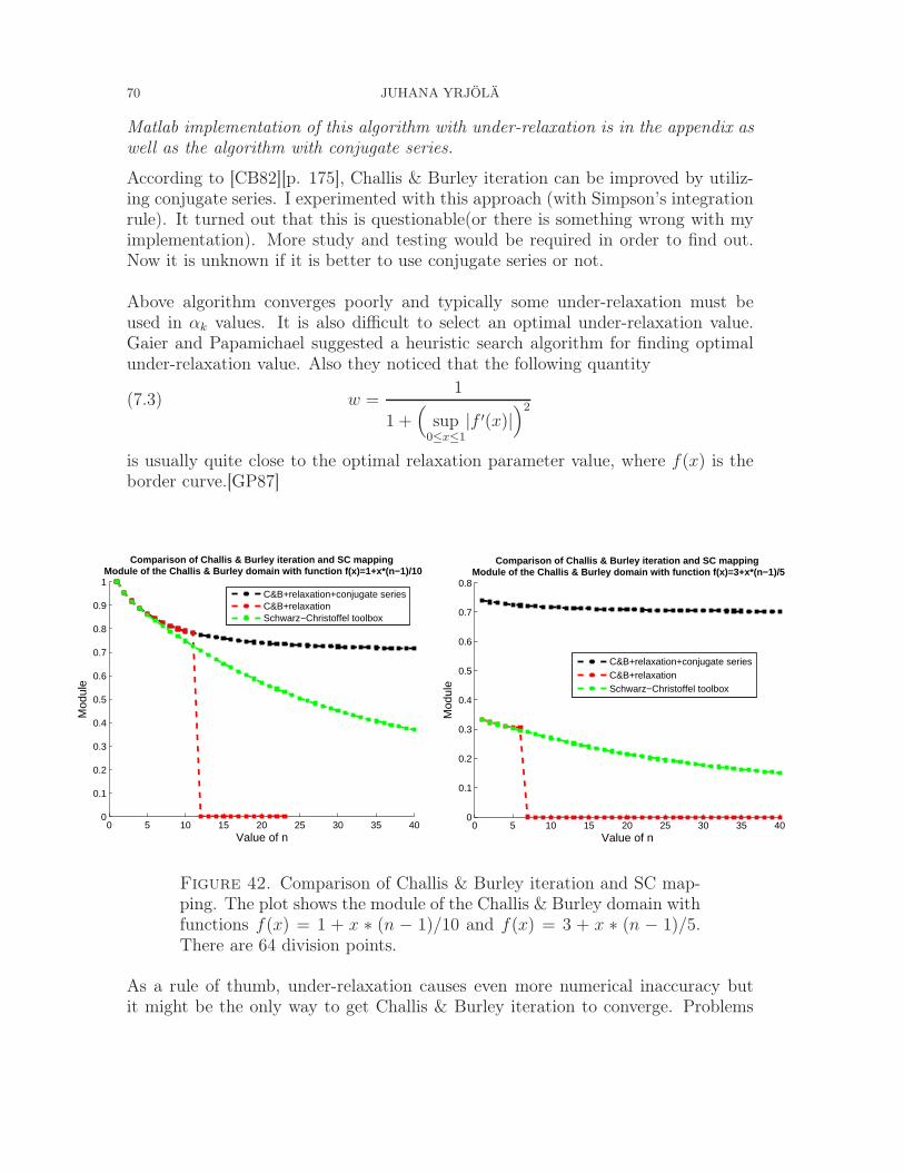
70 JUHANA YRJÖLÄ
Matlab implementation of this algorithm with under-relaxation is in the appendix aswell as the algorithm with conjugate series.
According to [CB82][p. 175], Challis & Burley iteration can be improved by utiliz-ing conjugate series. I experimented with this approach (with Simpson’s integrationrule). It turned out that this is questionable(or there is something wrong with myimplementation). More study and testing would be required in order to find out.Now it is unknown if it is better to use conjugate series or not.
Above algorithm converges poorly and typically some under-relaxation must beused in αk values. It is also difficult to select an optimal under-relaxation value.Gaier and Papamichael suggested a heuristic search algorithm for finding optimalunder-relaxation value. Also they noticed that the following quantity
(7.3) w =1
1 +(
sup0≤x≤1
|f ′(x)|)2
is usually quite close to the optimal relaxation parameter value, where f(x) is theborder curve.[GP87]
0 5 10 15 20 25 30 35 400
0.1
0.2
0.3
0.4
0.5
0.6
0.7
0.8
0.9
1
Comparison of Challis & Burley iteration and SC mapping Module of the Challis & Burley domain with function f(x)=1+x*(n−1)/10
Value of n
Mod
ule
C&B+relaxation+conjugate seriesC&B+relaxationSchwarz−Christoffel toolbox
0 5 10 15 20 25 30 35 400
0.1
0.2
0.3
0.4
0.5
0.6
0.7
0.8
Comparison of Challis & Burley iteration and SC mapping Module of the Challis & Burley domain with function f(x)=3+x*(n−1)/5
Value of n
Mod
ule
C&B+relaxation+conjugate seriesC&B+relaxationSchwarz−Christoffel toolbox
Figure 42. Comparison of Challis & Burley iteration and SC map-ping. The plot shows the module of the Challis & Burley domain withfunctions f(x) = 1 + x ∗ (n − 1)/10 and f(x) = 3 + x ∗ (n − 1)/5.There are 64 division points.
As a rule of thumb, under-relaxation causes even more numerical inaccuracy butit might be the only way to get Challis & Burley iteration to converge. Problems
NUMERICAL COMPUTATION OF THE MODULE OF A QUADRILATERAL 71
with Challis & Burley iteration and especially with relaxation are apparent fromthe Figure 42. The difference in accuracy between two different Challis & Burleyversions is due to relaxation value. Limited number of tests suggests that relaxedChallis & Burley behaves similar fashion than conjugate series without relaxation.This suggest that good relaxation values depend on the method and (7.3) is notoptimal for conjugate series.
7.2. Heikkala-Vamanamurthy-Vuorinen iteration.
Another method for the module computation is the Heikkala-Vamanamurthy-Vuorineniteration. This iteration is much more complex than the Challis & Burley iteration.The increase in the complexity comes from the fact that one needs to evaluate hy-pergeometric functions and elliptic integrals of the first kind. Also some kind of anumerical scheme must be used to find solution of the resulting equation. OriginallyNewton’s iteration was used for this purpose and hence the name iteration.
7.4. Definition (Gaussian hypergeometric function). [HVV04, p. 1]Given complex numbers a, b and c with c 6= 0,−1,−2, · · · , the Gaussian hyperge-ometric function is the analytic continuation to the slit plane C[1,∞) of the series
(7.5) F (a, b; c; z) =∞∑
n=0
(a, n)(b, n)
(c, n)
zn
n!, |z| < 1.
Here (a, 0) = 1 for a 6= 0, and (a, n) is the shifted factorial function or the Appellsymbol
(7.6) (a, n) = a(a + 1)(a + 2) · · · (a + n − 1),
for n ∈ N.
See [LO00] for a comprehensive list of papers on hypergeometric function and com-puter software used in numerical evaluation.
7.7. Theorem (Heikkala-Vamanamurthy-Vuorinen iteration for the elliptic modu-lus). [HVV04, p. 6]Let 0 < a < 1, 0 < b < 1, max a + b, 1 ≤ c ≤ 1 + min a, b, and let Q be aquadrilateral in the upper half plane with vertices 0,1,A and B, the interior anglesat which are, respectively, bπ, (c− b)π,(1− a)π and (1 + a− c)π.23Then the ellipticmodulus k satisfies the equation
(7.8) A = 1 +Lk′2(c−a−b)F (c − a, c − b; c + 1 − a − b; k′2)
F (a, b; c; k2),
where k′ =√
1 − k2 and
(7.9) L =B(c − b, 1 − a)
B(b, c − b)e(b+1−c)iπ.
23This is a convex quadrilateral. According to Vuorinen there is a chance that this result mighthold for non-convex domains too.
72 JUHANA YRJÖLÄ
For a proof see [HVV04].
In order to use above formula one must choose an initial guess for the k and theniterate for example by Newton’s method. When the elliptic modulus k is known,we can calculate the module of a quadrilateral by using equation (4.18), which isrepeated below
M(Q) =K
′(k)
2K(k).
Numerical methods for the evaluation of elliptic integrals of the first kind are dis-cussed in the appendix.
7.3. Numerical methods for solving partial differential equations.
There are two classical methods for finding a numerical solution to a partial differ-ential equation, namely the finite difference method(FDM) and the finite elementmethod(FEM). Usually the finite difference method is used for parabolic and hyper-bolic partial differential equations and finite element method is used for parabolicand elliptic equations24. Since the Laplace’s equation (3.39) is elliptic, finite elementmethods are generally more suitable for the module of a quadrilateral computationsthan finite difference methods. One open source finite element solver is Elmer,which has been developed by CSC (Finnish IT centre for science). For additionalinformation and downloads see
http://www.csc.fi/elmer/.
The first use of finite element method to compute the capacitance of condensers(andtherefore the module) was made by Gerhard Opfer in 1969. The basic finite elementmethod can be enhanced for the capacitance calculations. Betsakos, Samuelsson andVuorinen suggested applied finite element method(AFEM) in 2004, which accordingto their publication is reasonably fast and produces very accurate results. Thefinite element method and AFEM is beyond the scope of this text, for more detailssee [BSV04] and some finite element introduction text. Rasila and Vuorinen havedeveloped a web-browser based interface for AFEM, unfortunately this web-browserbased interface is not available to the public[RVI06].
24A partial differential equation of the form
(7.10) a∂2u
∂x2+ 2b
∂2u
∂x∂y+ c
∂2u
∂y2+ d
∂u
∂x+ e
∂u
∂y+ fu = g
is called a linear second-order partial differential equation with two variables x and y. If we replace∂u∂x
and ∂u∂y
by α and β respectively, we get the following equation
(7.11) P (α, β) = aα2 + 2bαβ + cβ2 + dα + eβ + f
The mathematical properties of the solutions of (7.10) are mainly determined by the algebraicproperties of the polynomial P (α, β). The partial differential equation (7.10) is classified as hyper-bolic, parabolic or elliptic according as its discriminant, b2−ac is positive, zero or negative.[DZ86,p. 4]
NUMERICAL COMPUTATION OF THE MODULE OF A QUADRILATERAL 73
List of special symbols and abbreviations
C The one point compactification of C, thus C = C ∪ ∞R
2 The one point compactification of R2, thus R
2 = R2 ∪ ∞
C Set of complex numbersR1 The two point compactification of R1, thus R1 = R1 ∪ ∞∪ −∞Γ A curve familyγ A curveK
′ Complete complementary elliptic integral of the first kind, K′ =
K(k′)K(k) Complete elliptic integral of the first kindM(Q) The module of the quadrilateral QN Set of natural numbers, N = 1, 2, 3, 4, · · · ∂D ∂D is the boundary of D, ∂D = D \ DR Set of real numbersρ∗ Extremal metricZ Set of integers, Z = · · · ,−2,−1,−1, 0, 1, 2, · · · Aρ(D) ρ-area of domain DD A domain is a open connected set in Rn or Cn
d(a, b) d(a, b) is a metric, ie the distance from a to bF (a, b; c; z) Gaussian hypergeometric functionF (k, φ) Elliptic integral of the first kindH+ The upper half-plane, H+ = (x, y) : x ∈ R, y ∈ R, y > 0k Elliptic modulusk′ Complementary elliptic modulus, k′ =
√1 − k2
Lρ(Γ) ρ-length of the curve family γlρ(γ) ρ-length of the curve γm(D, Γ) Module of the curve family Γ in domain Dodd Set of odd numbers, odd = 1, 3, 5, 7, 9, · · · P (Γ) Set of all admissible metrics for curve family ΓQ A quadrilateralR A region is an arbitrary set in Rn or Cn
Sτ upper Darboux sumsτ lower Darboux sumT A trilateral
74 JUHANA YRJÖLÄ
Appendix A. Numerical evaluation of the elliptic integrals of the
first kind
There are several methods for computing elliptic integrals of the first kind. Roughlyspeaking methods can be divided into two classes: methods for complete integralsonly and methods for both complete and incomplete integrals. The oldest methodsfor the computation of the elliptic integrals are almost as old as the elliptic inte-gral itself. Perhaps the oldest methods are from Gauss in 1799. Gauss discoveredfollowing series expansion for the complete elliptic integral of the first kind[MM99,pp. 66-67].
A.1. Theorem (Series expansion for complete elliptic integral of the first kind).[SL99, p. 195]
(A.2) K(k) =π
2
(
1 +(1
2
)2
k2 +(1 · 3
2 · 4)2
k4 +(1 · 3 · 5
2 · 4 · 6)2
k6 + · · ·)
where, k is the elliptic modulus and 0 < k < 1.
Gauss also discovered that arithmetic and geometric means can be used to evaluatethe Gauss’s trigonometric version of the complete integral. This method of Gausswas in reality disguised version of Landen’s transformation, which was published byEnglish mathematician John Landen in 1775.[MM99, pp. 66-67][EB, V16, p. 154]
A.3. Theorem (Method based on Landen’s transformation). [SL99, p. 196]
(A.4) F (k, φ) =
√
k1k2k3 · · ·k
ln tan(π
4+
φ
2
)
,
where k is the elliptic modulus and k < k1 < k2 < k3 < · · · < 1 and
(A.5) k1 =2√
k
1 + k, k2 =
2√
k1
1 + k1, · · · , ki+1 =
2√
ki
1 + ki
.
The product k1k2k3 · · · in (A.4) is considered as infinite product of ki, in other words∏i=∞
i=1 ki.
In order to use Landen’s transformation to get numerical values, we must fix indexi and compute the approximation value for F (k, φ) with fixed i. Landen’s transfor-mation converges reasonable well for elliptic integrals of the first kind.[NRC]
The most modern method currently available is by B. C. Carlson. Carlson intro-duced new versions of the integrals. These versions are called Carlson’s symmetricforms. Carlson’s symmetric form for elliptic integral of the first kind is
(A.6) RF (x, y, z) =1
2
∫ ∞
0
1√
(t + x)(t + y)(t + z)dt
NUMERICAL COMPUTATION OF THE MODULE OF A QUADRILATERAL 75
and RF (x, y, z) is related to K(k) and F (φ, k) by
K(k) = RF (1, 1 − k2, 0)(A.7)
F (φ, k) = sin (φ)RF
(
cos2(φ), 1 − k2 sin2 (φ), 1
)
.(A.8)
There are many versions of Carlson’s algorithms but the following algorithms workwith complex parameters.
A.9. Theorem (Carlson’s algorithm for K(k)). [Car94, p. 11]Let x0 = 1 and y0 =
√1 − k2. Now iterate by using following formulas
xm+1 =xm + ym
2m = 0, 1, 2, 3, · · · ,(A.10)
ym+1 =√
xmym, m = 0, 1, 2, 3, · · · ,(A.11)
and let xn and yn be final values of the iteration for fixed m then
(A.12) K(k) ≈ π
xn + yn
.
A.13. Theorem (Carlson’s algorithm for F (φ, k)). [Car94, p. 5]Set x0 = cos2 (φ), y0 = 1 − k2 sin2 (φ), z0 = 1 and A0 = x+y+z
3, then iterate for
m = 0, 1, 2, 3, · · · , n by using following formulas
λm =√
xm
√ym +
√xm
√zm +
√ym
√zm(A.14)
Am+1 =Am + λm
4(A.15)
xm+1 =xm + λm
4, ym+1 =
ym + λm
4, zm+1 =
zm + λm
4(A.16)
and let An be the final value of the iteration for fixed m and then calculate
X =A0 − x0
4nAn
, Y =A0 − y0
4nAn
, Z = −X − Y,(A.17)
E2 = XY − Z2, E3 = XY Z(A.18)
Then the value of F (φ, k) can be calculated from
(A.19) F (φ, k) ≈ sin (φ)A− 1
2n
(
1 − 1
10E2 +
1
14E3 +
1
24E2
2 −3
44E2E3
)
See [LO00] for a comprehensive list of papers on the elliptic integrals. The article[LO00] also helps in finding numerical libraries and other software packs for theevaluation of elliptic integrals(or for some other special function).
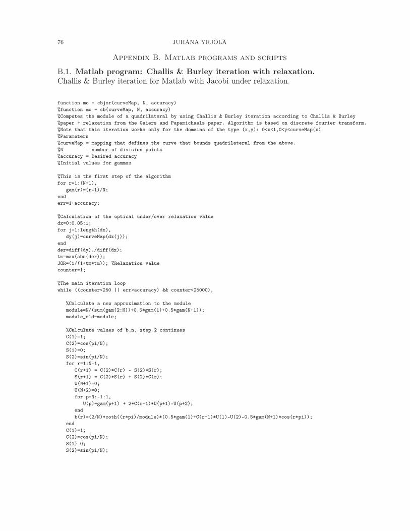
76 JUHANA YRJÖLÄ
Appendix B. Matlab programs and scripts
B.1. Matlab program: Challis & Burley iteration with relaxation.
Challis & Burley iteration for Matlab with Jacobi under relaxation.
function mo = cbjor(curveMap, N, accuracy)
%function mo = cb(curveMap, N, accuracy)
%Computes the module of a quadrilateral by using Challis & Burley iteration according to Challis & Burley
%paper + relaxation from the Gaiers and Papamichaels paper. Algorithm is based on discrete fourier transform.
%Note that this iteration works only for the domains of the type (x,y): 0<x<1,0<y<curveMap(x)
%Parameters
%curveMap = mapping that defines the curve that bounds quadrilateral from the above.
%N = number of division points
%accuracy = Desired accuracy
%Initial values for gammas
%This is the first step of the algorithm
for r=1:(N+1),
gam(r)=(r-1)/N;
end
err=1+accuracy;
%Calculation of the optical under/over relaxation value
dx=0:0.05:1;
for j=1:length(dx),
dy(j)=curveMap(dx(j));
end
der=diff(dy)./diff(dx);
tm=max(abs(der));
JOR=(1/(1+tm*tm)); %Relaxation value
counter=1;
%The main iteration loop
while ((counter<250 || err>accuracy) && counter<25000),
%Calculate a new approximation to the module
module=N/(sum(gam(2:N))+0.5*gam(1)+0.5*gam(N+1));
module_old=module;
%Calculate values of b_n, step 2 continues
C(1)=1;
C(2)=cos(pi/N);
S(1)=0;
S(2)=sin(pi/N);
for r=1:N-1,
C(r+1) = C(2)*C(r) - S(2)*S(r);
S(r+1) = C(2)*S(r) + S(2)*C(r);
U(N+1)=0;
U(N+2)=0;
for p=N:-1:1,
U(p)=gam(p+1) + 2*C(r+1)*U(p+1)-U(p+2);
end
b(r)=(2/N)*coth((r*pi)/module)*(0.5*gam(1)+C(r+1)*U(1)-U(2)-0.5*gam(N+1)*cos(r*pi));
end
C(1)=1;
C(2)=cos(pi/N);
S(1)=0;
S(2)=sin(pi/N);
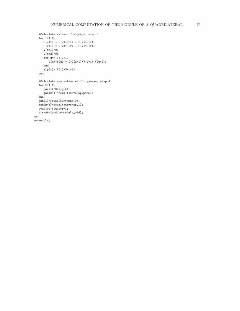
NUMERICAL COMPUTATION OF THE MODULE OF A QUADRILATERAL 77
%Calculate values of alpha_k, step 3
for r=1:N,
C(r+1) = C(2)*C(r) - S(2)*S(r);
S(r+1) = C(2)*S(r) + S(2)*C(r);
V(N+1)=0;
V(N+2)=0;
for q=N-1:-1:1,
V(q)=b(q) + 2*C(r+1)*V(q+1)-V(q+2);
end
alp(r)= V(1)*S(r+1);
end
%Calculate new estimates for gammas, step 4
for k=1:N,
para=k/N+alp(k);
gam(k+1)=feval(curveMap,para);
end
gam(1)=feval(curveMap,0);
gam(N+1)=feval(curveMap,1);
counter=counter+1;
err=abs(module-module_old);
end
mo=module;
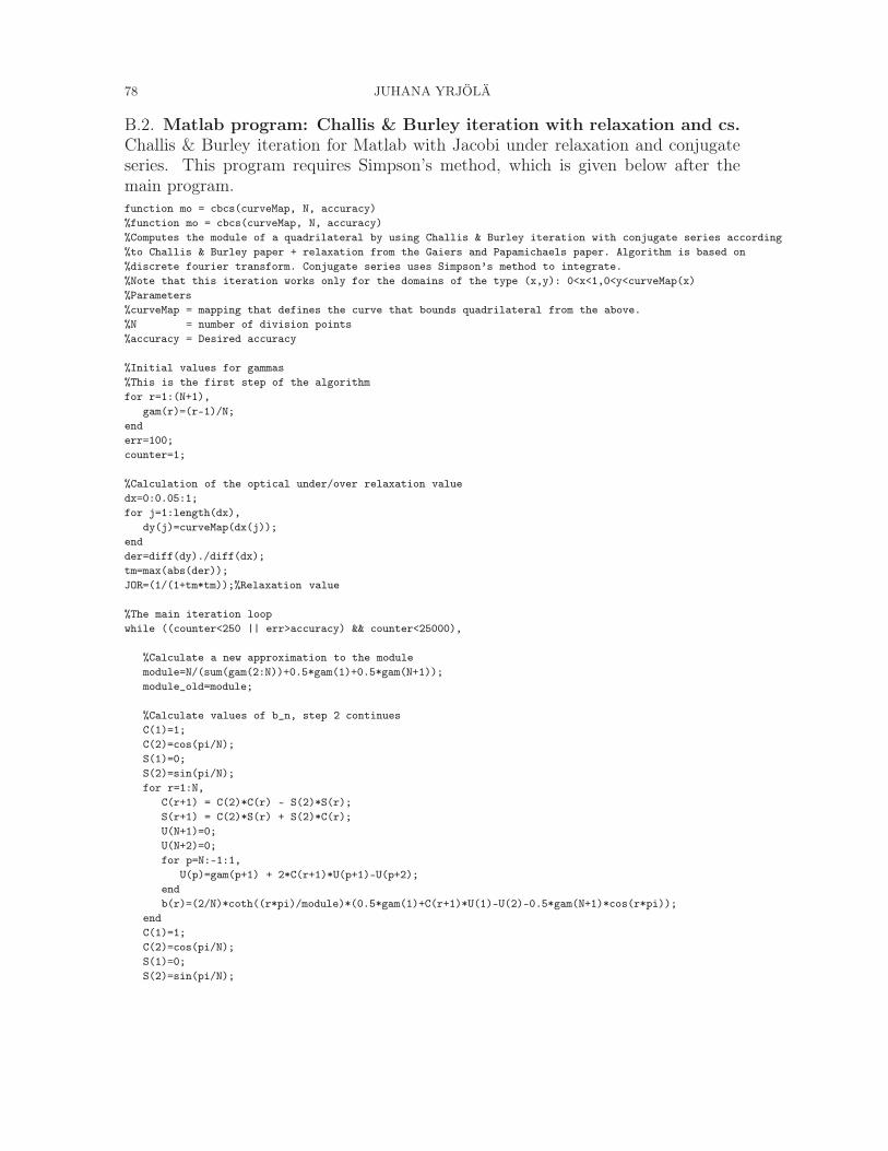
78 JUHANA YRJÖLÄ
B.2. Matlab program: Challis & Burley iteration with relaxation and cs.
Challis & Burley iteration for Matlab with Jacobi under relaxation and conjugateseries. This program requires Simpson’s method, which is given below after themain program.function mo = cbcs(curveMap, N, accuracy)
%function mo = cbcs(curveMap, N, accuracy)
%Computes the module of a quadrilateral by using Challis & Burley iteration with conjugate series according
%to Challis & Burley paper + relaxation from the Gaiers and Papamichaels paper. Algorithm is based on
%discrete fourier transform. Conjugate series uses Simpson’s method to integrate.
%Note that this iteration works only for the domains of the type (x,y): 0<x<1,0<y<curveMap(x)
%Parameters
%curveMap = mapping that defines the curve that bounds quadrilateral from the above.
%N = number of division points
%accuracy = Desired accuracy
%Initial values for gammas
%This is the first step of the algorithm
for r=1:(N+1),
gam(r)=(r-1)/N;
end
err=100;
counter=1;
%Calculation of the optical under/over relaxation value
dx=0:0.05:1;
for j=1:length(dx),
dy(j)=curveMap(dx(j));
end
der=diff(dy)./diff(dx);
tm=max(abs(der));
JOR=(1/(1+tm*tm));%Relaxation value
%The main iteration loop
while ((counter<250 || err>accuracy) && counter<25000),
%Calculate a new approximation to the module
module=N/(sum(gam(2:N))+0.5*gam(1)+0.5*gam(N+1));
module_old=module;
%Calculate values of b_n, step 2 continues
C(1)=1;
C(2)=cos(pi/N);
S(1)=0;
S(2)=sin(pi/N);
for r=1:N,
C(r+1) = C(2)*C(r) - S(2)*S(r);
S(r+1) = C(2)*S(r) + S(2)*C(r);
U(N+1)=0;
U(N+2)=0;
for p=N:-1:1,
U(p)=gam(p+1) + 2*C(r+1)*U(p+1)-U(p+2);
end
b(r)=(2/N)*coth((r*pi)/module)*(0.5*gam(1)+C(r+1)*U(1)-U(2)-0.5*gam(N+1)*cos(r*pi));
end
C(1)=1;
C(2)=cos(pi/N);
S(1)=0;
S(2)=sin(pi/N);
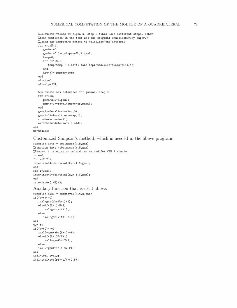
NUMERICAL COMPUTATION OF THE MODULE OF A QUADRILATERAL 79
%Calculate values of alpha_k, step 3 (This uses different steps, other
%than mentioned in the text see the original Challis&Burley paper.)
%Using the Simpson’s method to calculate the integral
for k=1:N-1,
gambar=0;
gambar=0.5*cbsimpson(k,N,gam);
temp=0;
for h=1:N-1,
temp=temp + b(h)*(1-tanh(h*pi/module))*sin(h*pi*k/N);
end
alp(k)=-gambar+temp;
end
alp(N)=0;
alp=alp*JOR;
%Calculate new estimates for gammas, step 4
for k=1:N,
para=k/N+alp(k);
gam(k+1)=feval(curveMap,para);
end
gam(1)=feval(curveMap,0);
gam(N+1)=feval(curveMap,1);
counter=counter+1;
err=abs(module-module_old);
end
mo=module;
Customized Simpson’s method, which is needed in the above program.function inte = cbsimpson(k,N,gam)
%function inte =cbsimpson(k,N,gam)
%Simpson’s integration method customized for C&B iteration
inte=0;
for r=2:2:N,
inte=inte+4*cbinteval(k,r-1,N,gam);
end
for r=3:2:N,
inte=inte+2*cbinteval(k,r-1,N,gam);
end
inte=inte*(1/N)/3;
Auxilary function that is used above.function ival = cbinteval(k,t,N,gam)
if((k+t)<=0)
ival=gam(abs(k+t)+1);
elseif((k+t)<N+1)
ival=gam(k+t+1);
else
ival=gam(2*N+1-t-k);
end
t2=-t;
if((k+t2)<=0)
ival2=gam(abs(k+t2)+1);
elseif((k+t2)<N+1)
ival2=gam(k+t2+1);
else
ival2=gam(2*N+1-t2-k);
end
ival=ival-ival2;
ival=ival*cot(pi*(t/N)*0.5);
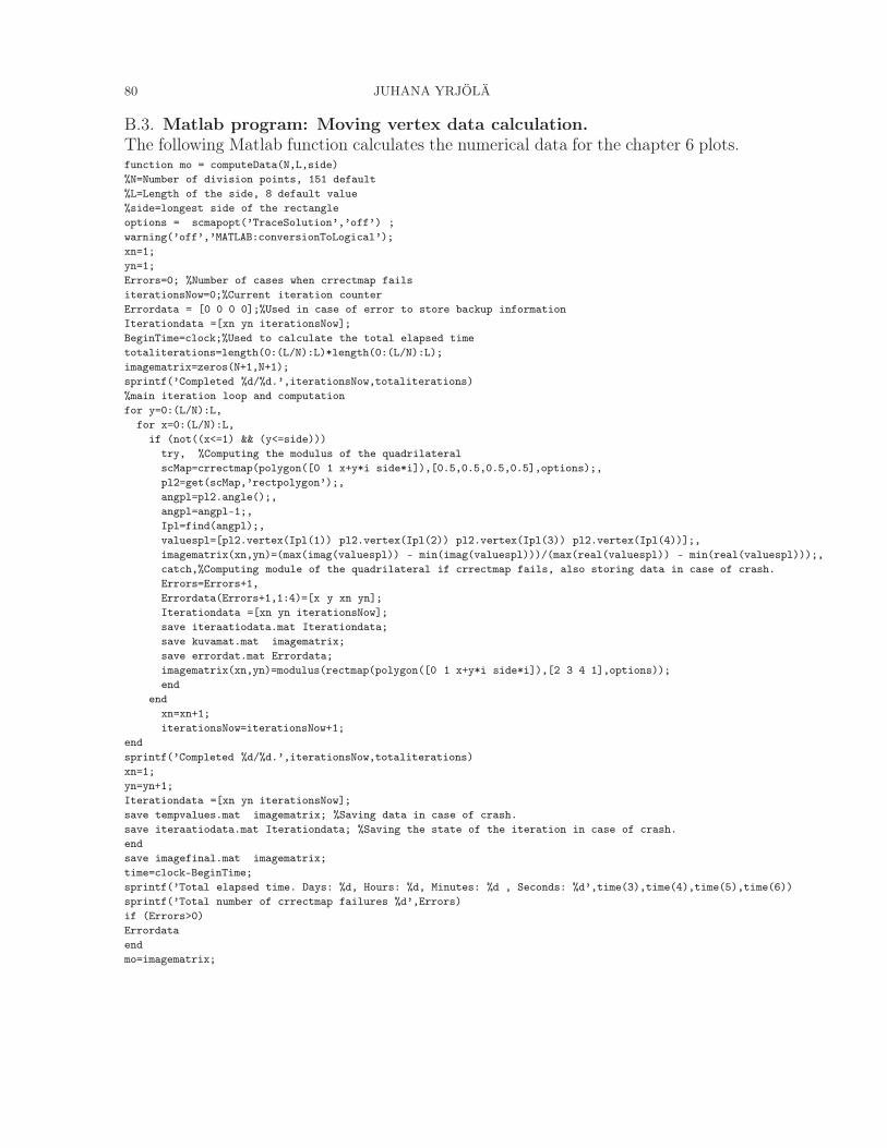
80 JUHANA YRJÖLÄ
B.3. Matlab program: Moving vertex data calculation.
The following Matlab function calculates the numerical data for the chapter 6 plots.function mo = computeData(N,L,side)
%N=Number of division points, 151 default
%L=Length of the side, 8 default value
%side=longest side of the rectangle
options = scmapopt(’TraceSolution’,’off’) ;
warning(’off’,’MATLAB:conversionToLogical’);
xn=1;
yn=1;
Errors=0; %Number of cases when crrectmap fails
iterationsNow=0;%Current iteration counter
Errordata = [0 0 0 0];%Used in case of error to store backup information
Iterationdata =[xn yn iterationsNow];
BeginTime=clock;%Used to calculate the total elapsed time
totaliterations=length(0:(L/N):L)*length(0:(L/N):L);
imagematrix=zeros(N+1,N+1);
sprintf(’Completed %d/%d.’,iterationsNow,totaliterations)
%main iteration loop and computation
for y=0:(L/N):L,
for x=0:(L/N):L,
if (not((x<=1) && (y<=side)))
try, %Computing the modulus of the quadrilateral
scMap=crrectmap(polygon([0 1 x+y*i side*i]),[0.5,0.5,0.5,0.5],options);,
pl2=get(scMap,’rectpolygon’);,
angpl=pl2.angle();,
angpl=angpl-1;,
Ipl=find(angpl);,
valuespl=[pl2.vertex(Ipl(1)) pl2.vertex(Ipl(2)) pl2.vertex(Ipl(3)) pl2.vertex(Ipl(4))];,
imagematrix(xn,yn)=(max(imag(valuespl)) - min(imag(valuespl)))/(max(real(valuespl)) - min(real(valuespl)));,
catch,%Computing module of the quadrilateral if crrectmap fails, also storing data in case of crash.
Errors=Errors+1,
Errordata(Errors+1,1:4)=[x y xn yn];
Iterationdata =[xn yn iterationsNow];
save iteraatiodata.mat Iterationdata;
save kuvamat.mat imagematrix;
save errordat.mat Errordata;
imagematrix(xn,yn)=modulus(rectmap(polygon([0 1 x+y*i side*i]),[2 3 4 1],options));
end
end
xn=xn+1;
iterationsNow=iterationsNow+1;
end
sprintf(’Completed %d/%d.’,iterationsNow,totaliterations)
xn=1;
yn=yn+1;
Iterationdata =[xn yn iterationsNow];
save tempvalues.mat imagematrix; %Saving data in case of crash.
save iteraatiodata.mat Iterationdata; %Saving the state of the iteration in case of crash.
end
save imagefinal.mat imagematrix;
time=clock-BeginTime;
sprintf(’Total elapsed time. Days: %d, Hours: %d, Minutes: %d , Seconds: %d’,time(3),time(4),time(5),time(6))
sprintf(’Total number of crrectmap failures %d’,Errors)
if (Errors>0)
Errordata
end
mo=imagematrix;
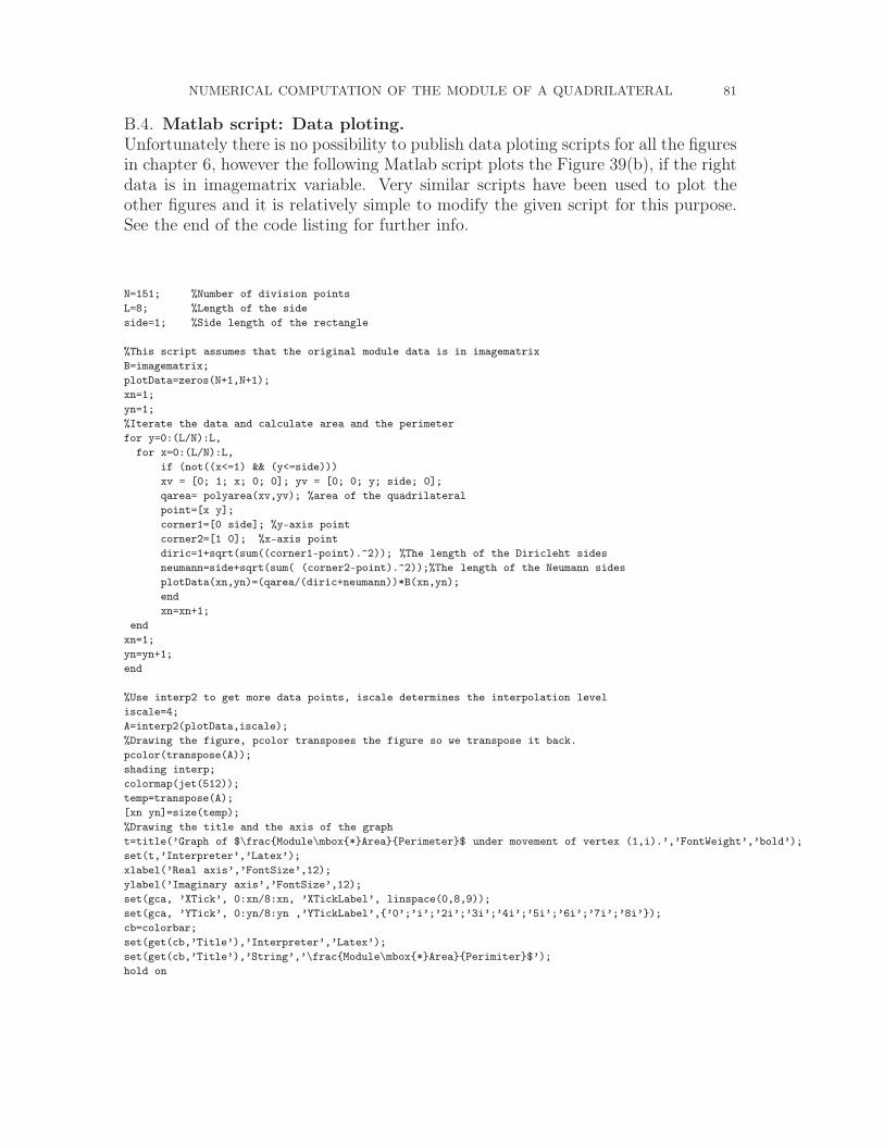
NUMERICAL COMPUTATION OF THE MODULE OF A QUADRILATERAL 81
B.4. Matlab script: Data ploting.
Unfortunately there is no possibility to publish data ploting scripts for all the figuresin chapter 6, however the following Matlab script plots the Figure 39(b), if the rightdata is in imagematrix variable. Very similar scripts have been used to plot theother figures and it is relatively simple to modify the given script for this purpose.See the end of the code listing for further info.
N=151; %Number of division points
L=8; %Length of the side
side=1; %Side length of the rectangle
%This script assumes that the original module data is in imagematrix
B=imagematrix;
plotData=zeros(N+1,N+1);
xn=1;
yn=1;
%Iterate the data and calculate area and the perimeter
for y=0:(L/N):L,
for x=0:(L/N):L,
if (not((x<=1) && (y<=side)))
xv = [0; 1; x; 0; 0]; yv = [0; 0; y; side; 0];
qarea= polyarea(xv,yv); %area of the quadrilateral
point=[x y];
corner1=[0 side]; %y-axis point
corner2=[1 0]; %x-axis point
diric=1+sqrt(sum((corner1-point).^2)); %The length of the Diricleht sides
neumann=side+sqrt(sum( (corner2-point).^2));%The length of the Neumann sides
plotData(xn,yn)=(qarea/(diric+neumann))*B(xn,yn);
end
xn=xn+1;
end
xn=1;
yn=yn+1;
end
%Use interp2 to get more data points, iscale determines the interpolation level
iscale=4;
A=interp2(plotData,iscale);
%Drawing the figure, pcolor transposes the figure so we transpose it back.
pcolor(transpose(A));
shading interp;
colormap(jet(512));
temp=transpose(A);
[xn yn]=size(temp);
%Drawing the title and the axis of the graph
t=title(’Graph of $\fracModule\mbox*AreaPerimeter$ under movement of vertex (1,i).’,’FontWeight’,’bold’);
set(t,’Interpreter’,’Latex’);
xlabel(’Real axis’,’FontSize’,12);
ylabel(’Imaginary axis’,’FontSize’,12);
set(gca, ’XTick’, 0:xn/8:xn, ’XTickLabel’, linspace(0,8,9));
set(gca, ’YTick’, 0:yn/8:yn ,’YTickLabel’,’0’;’i’;’2i’;’3i’;’4i’;’5i’;’6i’;’7i’;’8i’);
cb=colorbar;
set(get(cb,’Title’),’Interpreter’,’Latex’);
set(get(cb,’Title’),’String’,’\fracModule\mbox*AreaPerimiter$’);
hold on
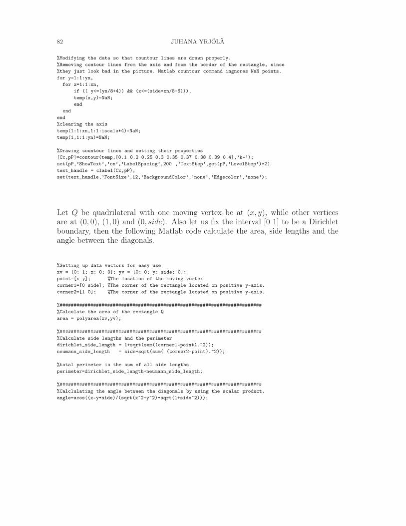
82 JUHANA YRJÖLÄ
%Modifying the data so that countour lines are drawn properly.
%Removing contour lines from the axis and from the border of the rectangle, since
%they just look bad in the picture. Matlab countour command ingnores NaN points.
for y=1:1:yn,
for x=1:1:xn,
if (( y<=(yn/8+4)) && (x<=(side*xn/8+6))),
temp(x,y)=NaN;
end
end
end
%clearing the axis
temp(1:1:xn,1:1:iscale*4)=NaN;
temp(1,1:1:yn)=NaN;
%Drawing countour lines and setting their properties
[Cc,pP]=contour(temp,[0.1 0.2 0.25 0.3 0.35 0.37 0.38 0.39 0.4],’k-’);
set(pP,’ShowText’,’on’,’LabelSpacing’,200 ,’TextStep’,get(pP,’LevelStep’)*2)
text_handle = clabel(Cc,pP);
set(text_handle,’FontSize’,12,’BackgroundColor’,’none’,’Edgecolor’,’none’);
Let Q be quadrilateral with one moving vertex be at (x, y), while other verticesare at (0, 0), (1, 0) and (0, side). Also let us fix the interval [0 1] to be a Dirichletboundary, then the following Matlab code calculate the area, side lengths and theangle between the diagonals.
%Setting up data vectors for easy use
xv = [0; 1; x; 0; 0]; yv = [0; 0; y; side; 0];
point=[x y]; %The location of the moving vertex
corner1=[0 side]; %The corner of the rectangle located on positive y-axis.
corner2=[1 0]; %The corner of the rectangle located on positive y-axis.
%########################################################################
%Calculate the area of the rectangle Q
area = polyarea(xv,yv);
%########################################################################
%Calculate side lengths and the perimeter
dirichlet_side_length = 1+sqrt(sum((corner1-point).^2));
neumann_side_length = side+sqrt(sum( (corner2-point).^2));
%total perimeter is the sum of all side lengths
perimeter=dirichlet_side_length+neumann_side_length;
%########################################################################
%Calclulating the angle between the diagonals by using the scalar product.
angle=acos((x-y*side)/(sqrt(x^2+y^2)*sqrt(1+side^2)));
NUMERICAL COMPUTATION OF THE MODULE OF A QUADRILATERAL 83
Appendix C. Other fields of interest
Here is a list of some properties that could be studied further. All these ideas havebeen thought to some extend, in the process of making this work but they have beenrejected because of usability issues or their being too complex and time consuming.Some of these ideas should be considered highly experimental and error prone.
C.1. General concepts and symmetry.
• It would be interesting to categorize domains according to the extremalmetric. As we know for a rectangle this extremal metric yields a constantin ρ-area and ρ-length integrals. What kind of domains would we get if wewould had x, x + x2 or something else in the integral? Perhaps it would beeven possible to derive some summation/other rules for the domains. Thismight also help to extend the generalized reflection symmetry Theorem toinclude fractions.
• The module under√
-map. There are some simple domains, which have
module√
2 or√
3 or something else. Perhaps with this data it would bepossible to come up with a model on how the module behaves under
√-map.
• It would be possible to study border rotations by drawing Matlab-figuresby using SC toolbox. The required script would be relatively simple. Onecould try to look for desymmetrization theorem for symmetric quadrilaterals.This theorem would transform symmetric quadrilaterals into nonsymmet-ric quadrilaterals with symmetric domain. This desymmetrization theoremwould explain the Figure 32.
• Derive a inequality(or equality) for the error term in rotation + glue trans-formation. See Example 5.16.
• Finding general formula for the mass addition to the symmetry axis or tosome other place. See Example 5.16.
• Least squares fit into some contour curves, which are given in the numericalresults section. One could study especially the generalized symmetry axis.
• Generalization of the reflection principle into domains without straight re-flection sides or some other reflection rules for the vertex placement.
• We have only looked at the simplest class of additive quadrilaterals, thosethat are formed by reflection. However there are probably a lot more suchclasses. One could start by looking at how non-symmetric boundary condi-tions with non-symmetrical area increase affect the module.
• It would be interesting to investigate reflections of domains with holes. Itmight be possible to use reflection property so that reflection to a domainwith a hole does not remove the other boundary condition and the domain isstill a quadrilateral with a hole and not a ring domain. Perhaps this wouldbe a topic that I would look into if I had more time.
84 JUHANA YRJÖLÄ
C.2. Numerical methods and Harmonic measure.
• It would be possible to construct a program that calculates the module ofa quadrilateral by trying out several different metrics and then selectingthe infimum value. This algorithm would produce approximate values inpractice.
Although this work did not cover harmonic measure at all, there are some interestingtopics that could be studied.
• Stochastically solve the Dirichlet-Neumann problem. There might be twoproblems in doing this. First, one needs to find the point from which therandom walk starts(it is clearly defined though see [Küh05, p. 118]), andsecondly, one needs to find the proper module formula for the particulardomain in question. In addition to that one must reflect the random walk ifit attempts to cross the Neumann sides.
• One topic could be to investigate the connection between the generalizedconformal center and the module of a quadrilateral. This topic was presentedby Iannaccone in his thesis[Ian03, p. 47] but apparently he did not pursue tostudy it. Perhaps this point could help picking the right start point for therandom walk. The SC toolbox can calculate the conformal center directlyso perhaps this topic could be studied even without the harmonic measure.
NUMERICAL COMPUTATION OF THE MODULE OF A QUADRILATERAL 85
References
[AB98] C. Aliprantis and O. Burkinshaw: Principles of real analysis, 3rd edition, Academicpress, 1998.
[AhBe50] L. Ahlfors and A. Beurling: Conformal invariants and function-theoretic null-sets,Acta Math. 83, pp. 101-129, 1950.
[BT03] L. Banjai and L. N. Trefethen: A Multipole Method For Schwarz Christoffel Mappingof Polygons With Thousands of Sides, SIAM Journal of Scientific Computing, Vol 25, No.3, pp. 1042-1065, 2003.
[BSV04] D. Betsakos, K. Samuelsson and M. Vuorinen: The computation of capacity ofplanar condensers, Publ. Inst. Math 75 (89)(2004),pp. 233-252
[CFP96] J. W. Cannon, W. J. Floyd, and W. R. Parry: Conformal modulus the graphpaper invariant or The conformal shape of an algorithm, 1996http://www.math.vt.edu/people/floyd/research/papers/conshape.html, Refer-enced [29.8.2006]
[Car94] B.C. Carlson: Numerical computation of real or complex elliptic integrals, Ames labo-ratory and department of mathematics, Iowa State University.
[CB82] N. V. Challis and D. M. Burley: A Numerical Method for Conformal Mapping, IMAJournal of Numerical Analysis 2, pp. 169-181, 1982.
[DV98] T. A. Driscoll and S. A. Vavasis: Numerical Conformal Mapping Using Cross-Ratiosand Delaynay Triangulation, SIAM Journal of Scientific Computing,Vol. 19, No. 6, pp.1783-1803, 1998
[SCTUG] T. A. Driscoll: Schwarz-Christoffel Toolbox User’s Guide, version 2.3, Departmentof Mathematical Sciences, Ewing Hall, University of Delaware, Newark, DE 19716.
[Dri02] T.A. Driscoll and L.N. Trefethen Schwarz-Christoffel Mapping, Cambridge univer-sity press, Cambridge, 2002.
[DV05] V. N. Dubinin, M. Vuorinen: On conformal moduli of polygonal quadrilaterals,Preprint 417, University of Helsinki, 12 pp. arXiv math.CV/0701387, 2005http://mathstat.helsinki.fi/reports/Preprint417.pdf Referenced [10.11.2006]
[DZ86] P. DuChateau and D. Zachmann: Schaum’s outlines Partial Differential Equations,McGraw-Hill, 1986.
[EP02] J. F. Epperson: An Introduction to Numerical Methods and Analysis, John Wiley &Sons, New York, 2002
[Fla83] F.J. Flanigan: Complex variables, harmonic and analytic funtions, Dover, New York,1983.
[Gai79] D. Gaier: Capacitance and the conformal Module of a Quadrilaterals, Journal of math-ematical analysis and applications 70, pp.236-239, 1979
[GP87] D. Gaier and N. Papamichael: On the Comparison of Two Numerical Methods forConformal Mapping, IMA Journal of Numerical Analysis 7, pp. 261-282, 1987.
[HVV04] V. Heikkala, M. K. Vamanamurthy and M. Vuorinen: Generalized elliptic inte-grals- Preprint 404, University of Helsinki 30 pp. arXiv math.CA/0701436, 2004.
[Hen74] P. Henrici: Applied and Computational Complex Analysis, Volume 1: Power series,Integration, Conformal Mapping, Location of Zeros., Wiley, New York, 1974.
[Hen91] P. Henrici Applied and Computational Complex Analysis: Special Functions, IntegralTransforms, Asymptotics, Continued Fractions Vol 2 (Classics Library), John Wiley &Sons Inc, 1991.
[How90] L. H. Howell: Computation of Conformal Maps by Modified Schwarz-Christoffel Trans-formations, Partial fulfillment of the requirements for the degree of Doctor of Philosophy,Massachusetts Institute of Technology, 1990.
86 JUHANA YRJÖLÄ
[Ian03] A. Iannaccone: Senior Thesis: The conformal Center of a Triangle or a Quadrilat-eral, Harvey Mudd College, 2003 http://www.math.hmc.edu/math197/archives/2003/
aiannacc/aiannacc-2003-thesis.pdf Referenced [10.11.2006][Kre05] E. Kreyszig: Advanced Engineering Mathematics 9th edition, Wiley , 2005[Küh05] R. Kühnau Handbook of complex analysis: Geometric function theory, Volume 2, Else-
vier, 2005.[LV73] O. Lehto and K. I. Virtanen: Quasiconformal mappings in the plane, Springer, Berlin,
1973.[Loe59] C. Loewner: On conformal capacity in space, J. Math. Mech.(Nowadays Indiana Univ.
Math J.) 8, pp. 411-414, 1959[LO00] D. W. Lozier and F. W. J. Olver: Numerical evalutation of special functions, 2000
http://math.nist.gov/mcsd/Reports/2001/nesf/ Referenced [10.11.2006][MM99] H. McKean and V. Moll: Elliptic Curves: Function theory, Geometry, Arithmetic,
Cambridge University Press, Cambridge, 1999[PS88] N. Papamichael and N. S. Stylianopoulos: On a Domain decomposition method for
the computation of conformal modules, Numer. Math. 62 pp. 213-234, 1988.[PS92] N. Papamichael and N. S. Stylianopoulos: A Domain Decomposition method for
approximating the conformal modules of long quadrilaterals, Appl. Math. Lett. Vol 1, No.3,pp. 277-280, 1992.
[PS99] N. Papamichael and N. S. Stylianopoulos: The Asymptotic Behavior of Confor-mal Modules of Quadrilaterals with Applications to the Estimation of Resistance Values,Constructive Approximation 15, Springer-Verlag, New York, pp. 109-134, 1999
[Por06] R. M. Porter: History and Recent Developments in Techniques for Numerical Confor-mal Mapping, Proceedings of the International Workshop on Quasiconformal Mappingsand their Applications, 2006
[RVI06] A. Rasila and M. Vuorinen: Experiments with moduli of quadrilaterals - Rev.Roumaine Math. Pures Appl. 51 (2006) 747-757. arXiv math.NA/0703149, 2006
[RVII06] A. Rasila and M. Vuorinen: Experiments with moduli of quadrilaterals II.- Manu-script, 10 pp, 2006
[Spi99] M. R. Spiegel: Schaum’s outlines Complex variables with an Introduction to conformalmapping and its applications, McGraw-Hill, 1999.
[SL99] M. R. Spiegel and J. Liu: Mathematical handbook of formulas and tables, McGraw-Hill,1999.
[Vas02] A. Vasil’ev: Moduli of Families of curves for Conformal and Quasiconformal Mappings,Springer, Berlin, 2002.
[Väi71] J. Väisälä Lectures on n-Dimensional quasiconformal mappings, Springer-Verlag, Berlin,1971.
[EB] 1911 Encyclopedia Britannicahttp://encyclopedia.jrank.org/, Referenced [18.8.2006]
[ENC89] Encyclopaedia of mathematics, Kluwer academic publishers, Dordrecht, 1989.[NRC] Numerical Recipes in C
http://www.library.cornell.edu/nr/bookcpdf.html, Referenced [7.11.2005]
Index
Abel Niels, 16accuracy of the SC toolbox, 38additive quarilaterals, 55admissible metric, 20Ahlfors Lars, 18amplitude, 16analytic continuation, 39analytic function, 6annulus, 53Appell symbol, 71applied finite element method(AFEM), 72aspect ratio, 25, 39
Beurling Arne, 18boundary condition, 10
capacitance of the condenser, 38Carathéodory Constantin, 12Carathéodory-Osgood Theorem, 14, 28Carlson, 74Cauchy-Riemann equations, 6Challis & Burley iteration, 68Christoffel Elwin, 27closed curve, 7complementary elliptic modulus, 16complete elliptic integral of the first kind,
16, 17complex numbers, 5compound Gauss-Jacobi quadrature, 32conformal center, 84conformal equivalence, 13conformal equivalence with vertices, 14conformal invariant, 21, 22conformal mapping, 11conjugate functions, 6connected set, 8CRDT, 32cross ratio, 13cross-ratios and Delaunay triangulations, 32crowding, 32CSC, 72curve, 7curve family, 7
Darboux Gaston, 15Darboux lower integral, 16Darboux lower sum, 15Darboux upper integral, 16Darboux upper sum, 15
Davis’s iteration, 30derivative, 6Dirichlet boundary condition, 10Dirichlet’s problem, 10Dirichlet-Neumann problem, 10domain, 8domain decomposition, 32Driscoll, 32
elliptic integral of the first kind, 16elliptic integrals, 16elliptic modulus, 16elliptic PDE, 72Elmer, 72extremal length, 18, 20extremal metric, 20
finite difference method, 72finite element method, 72Fuglede Bengt, 19
Gauss Carl, 10, 16, 74generalized conformal center, 84generalized quadrilateral, 9, 14GUI, 35
harmonic function, 6harmonic measure, 18, 51, 84Heikkala-Vamanamurthy-Vuorinen iteration,
71hyperbolic PDE, 72hypergeometric function, 71
Jacobi Carl, 16Johansson Severin, 12Jordan Camille, 8Jordan curve, 8Jordan curve Theorem, 9Jordan domain, 9
Landen John, 74Landen’s transformation, 74Laplace’s equation, 6, 72Legendre Adrien-Marie, 16Leibniz Gottfried, 6lemniscate, 16length of curve, 7Linux, 54Loewner, 25
87
88 JUHANA YRJÖLÄ
Möbius transformation, 13, 34machine epsilon, 17Matlab, 35, 54method of Garrick, 68metric, 7metric space, 7Mizar, 9module, 14module formula, 20module line, 23module of a curve family, 18module of a quadrilateral, 18, 22, 54module of the curve family, 20moduli, 18modulus, 18multiply connected, 8
Neumann boundary condition, 10Neumann’s problem, 10Newton Isaac, 6Newton’s method, 72non-rectifiable, 7numerical integration, 32
Opfer Gerhard, 72
parabolic PDE, 72parameter problem, 29partial differential equation, 9, 72path, 7pathwise connected, 8Plato, 7prevertex, 28
quadrilateral, 9quasiconformal mapping, 54
random walk, 18Rasila Antti, 68, 72reciprocal module, 22rectangle, 16rectifiable, 7region, 8Rengel’s inequality, 25Riemann, 14, 27Riemann integrable, 16Riemann’s mapping theorem, 12, 27ring domain, 53roundoff error, 18
Schwarz Hermann, 27Schwarz’s reflection principle, 40
Schwarz-Christoffel Mapping, 27Schwarz-Christoffel Toolbox, 32, 35, 54side of the quadrilateral, 9side-length method, 31simple curve, 8simply connected, 8special function, 75stochastic proceses, 18symmetric quadrilateral, 41, 42symmetry axis, 41, 59
tilings of a square, 44Trefethen Nick, 31trilateral, 9, 14truncation error, 18
under-relaxation, 70unstable, 18
Vavasis, 32Veblen Oswald, 9vertex, 9Vuorinen Matti, 71, 72