numerical characterisation of slug flow in horizontal … · horizontal air /water pipe flow ......

$: NUMERICAL CHARACTERISATION OF SLUG FLOW IN HORIZONTAL … · HORIZONTAL AIR /WATER PIPE FLOW ... The objective has been to investigate the volume fraction profile and pressure variation,$
© 2016 WIT Press, www.witpress.comISSN: 2046-0546 (paper format), ISSN: 2046-0554 (online), http://www.witpress.com/journalsDOI: 10.2495/CMEM-V4-N2-114-130

Z. I. Al-Hashimy et al., Int. J. Comp. Meth. and Exp. Meas., Vol. 4, No. 2 (2016) 114–130

NUMERICAL CHARACTERISATION OF SLUG FLOW IN HORIZONTAL AIR/WATER PIPE FLOW

ZAHID I. AL-HASHIMY1*, HUSSAIN H. AL-KAYIEM2, RUNE W. TIME3 & ZENA K. KADHIM4

1,2Mechanical Engineering Department, Universiti Teknologi PETRONAS, 32610 Tronoh, Perak, Malaysia. 3Department of Petroleum Engineering, Faculty of engineering and Science, University of Stavanger, Norway.

4Mechanical Engineering Department, College of Engineering, Wasit University, Wasit, Iraq.

ABSTRACTIn this work, the slug flow regime in an air-water horizontal pipe flow has been simulated using the CFD technique. The variables identified to characterise the slug regime are the slug length and slug ini-tiation. Additionally, the pressure drop and the pressure distribution within the simulated pipe segment have been predicted. The volume of fluid method was employed assuming unsteady, immiscible air-water flow, constant fluid properties and coaxial flow. The model was developed in the STAR-CCM+ environment, and the grid was designed in the three dimensional domain using directed mesh. A grid independency study was carried out through the monitoring of the water velocity at the outlet section. 104,000 hexahedral cells for the entire geometry were decided on as the best combination of comput-ing time and accuracy. The simulated pipe segment was 8 m long and had a 0.074 m internal diameter. Three cases of air-water volume fractions have been investigated, where the water flow rate was pre-set at 0.0028 m3/s, and the air flow rate was varied at three dissimilar values of 0.0105, 0.0120 and 0.015 m3/s. These flow rates were converted to superficial velocities and used as boundary conditions at the inlet of the pipe. The simulation was validated by bench marking with a Baker chart, and it had success-fully predicted the slug parameters. The computational fluid dynamics simulation results revealed that the slug length and pressure were increasing as the air superficial velocity increased. The slug initiation position was observed to end up being shifted to a closer position to the inlet. It was believed that the strength of the slug was high at the initiation stage and reduced as the slug progressed to the end of the pipe. The pressure gradient of the flow was realised to increase as the gas flow rate was increasing, which in turn was a result of the higher mean velocity.Keywords: hexahedral mesh, slug flow, slug flow characteristics, superficial velocity, two-phase flow.

1 INTRODUCTIONThe growth of liquid slugs in oil and gas pipelines is a vast and costly problem for the oil firms. A pressure drop in oil production is the main source of the problem that leads to terrain-induced slug flow in the pipeline between the production platform and wellhead plat-form. This type of slug flow condition can create huge transient surges. The transient nature of the slugs if not appropriately considered might become climacteric and can hasten the material’s fatigue with the risk of pipe damage and maintenance costs.

Recently, with the development of a programming and computation method, the computa-tional fluid dynamics (CFD) has been widely used to investigate the behaviour and describe the regime of the two-phase flow. However, modelling and simulating the two-phase flow to determine the distribution of the liquid and the gas phases is tedious work and is still consid-ered as challenge to the researchers due to the huge uncertainty that is encountered in terms of physics and mathematics. The phase distribution plays a major role in the designing of many engineering structures because it affects the values of several parameters, such as pres-sure drop and thermal load; therefore, it is necessary to determine the distribution and specify the flow regime that may exist in the system. Two phase-flow maps are useful tools because they facilitate the process of defining the flow pattern that exists under various boundary conditions without having to perform comprehensive numerical calculations [1].

Z. I. Al-Hashimy et al., Int. J. Comp. Meth. and Exp. Meas., Vol. 4, No. 2 (2016) 115

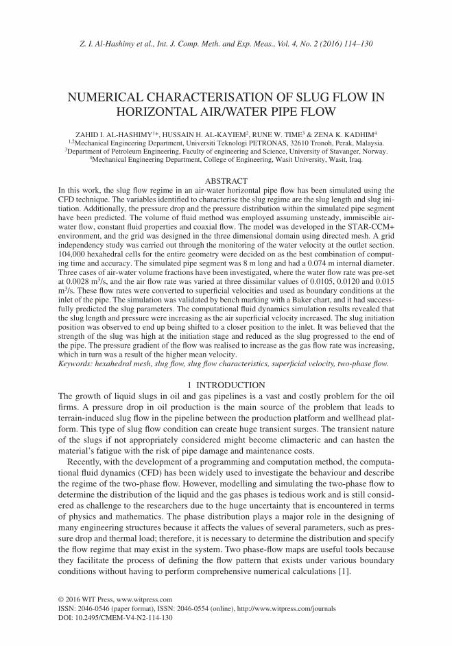
The slug formation is a three-step process that is depicted in Fig. 1. Originally, the flow is stratified where the gas is at the top of the pipe and the liquid at the bottom. As the gas passes over a wave, there is a pressure drop, then a pressure recovery, creating a small force upward within the wave. Under the conditions that this upward force is sufficient to raise the wave until it extends to the top of the pipe, the flow is considered as slug flow. Once the wave reaches the top of the pipe, it forms into the familiar slug shape with a nose and tail. The slug is forced forward by the gas and thus, can travel at a greater velocity than the liquid film [2].

The actual slug movement can be explained by changing the liquid slugs and the gas bub-bles moving above the liquid films, which in turn combine to develop what is known as a slug unit. The slug frequency is described by the number of slugs passing a particular point along the pipeline over a particular period of time. Amongst the slug flow characteristics, the slug frequency is an essential component which relates to significant operational difficulties, like the flooding of downstream facilities, severe pipe vibration, pipeline structural instability and wellhead pressure fluctuation. It is generally known that pipe corrosion is substantially impacted by a high slug frequency [3].

Slug flow refers to the phenomenon at which two-phase liquid-gas movements exist in pipelines over a broad range of intermediate flow rates, generating improper disorder result-ing from the actions of the liquid and gas plugs, known as slugs. The plug distribution of liquids and gases in slug flows are highly unique but intermittent, basically because of the nature of the terrain, gas/liquid velocity fluctuations, pigging, etc. A slug unit consists of an aerated liquid slug as well as an accompanying gas bubble, controlled within a liquid film of varying thicknesses. The actual thickness of the film in most cases differs from the minimum value at the front of the following slug towards the maximum value at the rear of the preced-ing slug. Consequently, the slug length may remain steady along the direction of travel while the pressure drops systematically across the sections of the pipe [4].

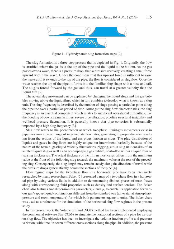
Flow regime maps for the two-phase flow in a horizontal pipe have been intensively researched by many researchers. Baker [5] presented a map of a two-phase flow in a horizon-tal pipe by using various fluids in addition to demonstrating distinct phases of mass fluxes along with corresponding fluid properties such as density and surface tension. The Baker chart also features two dimensionless parameters, l and y, to enable its application for vari-ous gas/vapour-liquid combinations different from the standard one (air-water at atmospheric pressure and room temperature) for which both parameters equate to unity. The Baker chart was used as a reference for the simulation of the horizontal slug flow regimes in the present study.

In this present work, the Volume of Fluid (VOF) method has been implemented employing the commercial software Star-CCM+ to simulate the horizontal sections of a pipe for air-wa-ter slug flow. The objective has been to investigate the volume fraction profile and pressure variation, with time, in seven different cross sections along the pipe. In addition, the pressure

Figure 1: Hydrodynamic slug formation steps [2].

116 Z. I. Al-Hashimy et al., Int. J. Comp. Meth. and Exp. Meas., Vol. 4, No. 2 (2016)

drop along 8 m of the pipe length will be predicted by the simulation. The Baker chart was adopted to justify the slug presence in the simulation by computing the superficial mass velocities of the water and air. The simulated horizontal slug flow patterns observed through visualizations of the phase distributions were qualitatively compared against the flow regimes expected by the Baker chart.

2 PROBLEM FORMULATIONThe Baker flow regime map, demonstrated in Fig. 2, shows the standardised boundaries of the various flow pattern regions as functions of the mass flux of the gas phase, G, and the ratio of the mass flux of the water phase and air, L/G. Where, G was the mass flux of the gas phase (kg/m2 s) = (gas mass flow rate/tube cross-sectional area) and L was the mass flux of water phase (kg/m2s) = (water mass flow rate/tube cross-sectional area). The dimensionless param-eters, l and y, had been added so that the chart could be utilised for any gas/liquid combination that differed from the standard combination. The standard combinations, at which both parameters, l and y, equate to unity, which are water and air flow under atmos-pheric pressure and at room temperature. Consequently, for the present application, where the fluids were air and water, the values of l and y are equal to 1.0. By taking into account, the predicted values for l and y, the pattern of the two-phase flows with any gas/liquid at other pressures and temperatures can be forecasted using the same chart. The parameters l and y were can be calculated from eqns (1) and (2):

Y =

ss

mm

rr

w l

w

w

l

21

3

(1)

l r

rr

r=

.

g

a

l

w

0 5

(2)

Where σ, μ, ρ are the surface tension, viscosity and density, respectively. The subscripts ‘a’ and ‘w’ refers to the air and water, respectively, at normal temperature and atmospheric pres-sure; whereas, the subscripts ‘g’ and ‘l’ refers to the vapour and liquid conditions of the fluid being considered.

Using the physical properties of air-water, shown in Table 1, the superficial velocities for both phases were extracted from the Baker chart slug zone. By imposing the intersection of the points within the slug regime in the Baker chart, as shown in Fig. 2, the values of G were found as 2.993, 3.42 and 4.275 kg m−2 s−1. Then, the air superficial velocities, Usa, were obtained from G/ra, as 2.443, 2.792 and 3.49 m/s, respectively. Eventually, the water superficial velocity, Usw, was predicted as 0.651 m/s, where G = 2.993 and L/G = 217.117 from L/rw.

Table 1: Physical properties for air and water.

Fluid Density r [kg/m3] Viscosity μ [Pa∙s] Surface tension s [N/m]

Water 998.2 1.003×10−3 0.07194Air 1.225 1.8551×10−5 –


3 COMPUTATIONAL SIMULATION PROCEDUREA CFD technique has been utilised to simulate the air-water slug flow in a horizontal pipe using STAR-CCM+ commercial software. It was experienced that this software was able to simulate well the complex flow phenomenon, like the slug flow. The summary of the sequence of the simulation procedure is:

• Generate CAD model according to pipe geometries.

• Specify the boundary conditions, which are velocity inlet and pressure outlet.

• Select the appropriate meshing criteria and mesh size, and conduct the mesh independency check.

• Select the physics of the model (turbulent models, flow regime, multiphase…etc.

• Specify the time step and physical time of the simulation.

• Create result reports and plots.

• Analyze the results.

Below is a detailed description of the numerical procedure of the present work.

3.1 Geometry

The model of the pipe is shown in Fig. 3. The pipe is horizontal with a diameter, DP, of 0.074 m and a length, LP, of 108 DP.

3.2 Boundary conditions

The required boundary conditions depend on the physical models used. Water was designated as the primary phase and air as the secondary phase for all cases. The water and air were

Figure 2: Baker chart. (•) Operating conditions of water–air two-phase flow [5].


considered incompressible. The most suitable boundary condition for external faces in incompressible water was the velocity inlet. The outlet was considered as a pressure-outlet boundary [6]. The boundary conditions used are illustrated schematically in Fig. 4.

There were two methods used in specifying the inlet boundary conditions for the simula-tion of the slug flow [7]. The first method imposed perturbations at the inlet so that the volume fraction of the liquid phase entered the pipe as a function of time as shown in Fig. 5. This function was expressed by using the Water Level, y1:

y y AU t

psw

1 0 11

2= +

sin

.p (3)

Where y0 = 0.0, A1 = 0.25DP, p1= 0.25LP.In the second method, the pipe was initially assumed to be filled with stratified air and

water with 50% volume percentage and zero velocity. For the present simulation, the initial and inlet region were: the upper half of the pipe was occupied by 50% void frac-tion of the gas phase, aa and the lower half by 50% volume fraction of the water phase, aw. Then, the field function was used to define the inlet water volume fraction as a func-tion of time.

Based on the Baker chart, presented in Fig. 2, the superficial velocities for the air and water phases were set as initial and inlet velocities, as shown in Table 2. Consequently, the mixture velocity, UM, resulted from the sum of the air superficial velocity, Usa, and the water super-ficial velocity, Usw. So, UM always has a value greater than the air and water superficial velocities.

Figure 3: Pipe geometry modelled in the STAR-CCM+.

Figure 4: Boundary condition for water-air slug flow through a pipe.


3.3 Meshing criteria

The mesh is an integral part of the numerical solution and must satisfy certain criteria to ensure an accurate solution. In this work, the mesh was developed using the Directed Mesh technique in Star-CCM+. Directed Mesh technique was proved to be suitable to simulate a two-phase flow in a horizontal pipe [7]. This technique was selected based on its effective-ness in reducing the number of cells and computational time with respect to other meshing techniques. It has tools which offer the ability to parametrically create grids from geometry in a multi-block structure. Where, by using the path mesh, the user can control and specify the number of divisions in the inlet cross section to generate quadrilateral faces; and using a new volume distribution, the user has the option to specify the number of layers along the pipe. After that we choose generate volume mesh. The hexahedral grid cells were generated by extruding quadrilateral faces from the inlet of the pipe along the length of the pipe at each layer.

A structured hexahedral grid was more suitable when solving the case under study since there was more control to obtain a fine cross-sectional mesh without the need to have an equivalent longitudinal one. As a result, it would make the solution’s process convergence faster. The fluid domains were not considered as symmetrical.

A grid independency study was conducted based on monitoring the water superficial velocity at the outlet section. The superficial velocity in a multiphase flows is defined as the ratio of the velocity and the volume fraction of the considered phase in a multiphase system. Actual velocity of phase = (Superficial velocity of phase)/(volume fraction of phase). The

Figure 5: Water phase entering the pipe as a function of time according to eqn (3).

Table 2: The superficial velocities for the simulation cases.

Air-water cases

Water superficial velocity (m/s)

Air superficial velocity (m/s)

Mixture velocity (m/s)

Case 10.651

2.443 3.049Case 2 2.792 3.443Case 3 3.49 4.141


average velocity of the flow varied depending on the volume fraction of each phase; which, when defined as the area fraction of a phase, is expected to change in space and time. The average velocity for the gas phase and liquid phase, which are called the gas superficial veloc-ity and liquid superficial velocity, can be given by [8]:

U

U A

AUSG

G GG G= = a

(4)

U

U A

AUSW

W WW W= = a

(5)

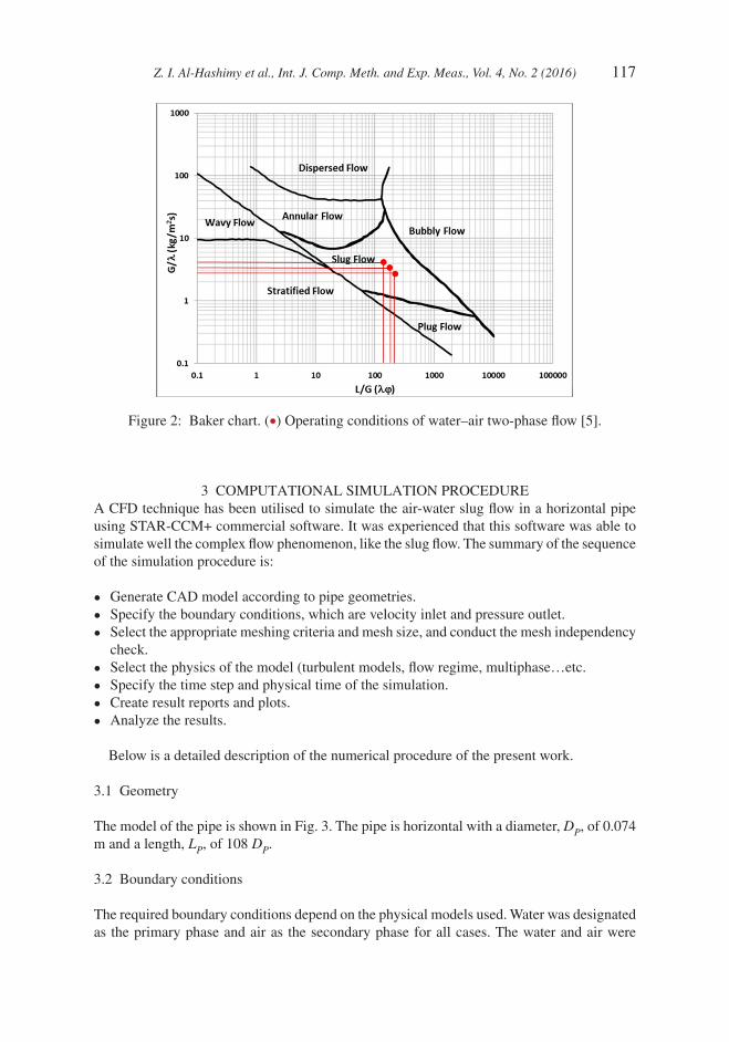
Four mesh sizes have been checked. The mesh with 52,000 cells was increased gradually to 78,000, 104,000 and 312,000. As seen in Fig. 6, increasing the number of elements from 104,000 to 312,000 resulted in a 0.6 % difference in the water velocity at the outlet section, which was small. Hence, 104,000 elements were used as the compromising number between the accuracy and the computational time.

Figure 6: Mesh sensitivity analysis.

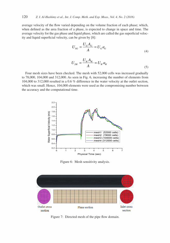
Figure 7: Directed mesh of the pipe flow domain.


The final mesh adopted to perform the full 3D volume simulations was divided into 104,000 hexahedral cells; 300 grid cells were used in a cross section and 350 grid cells in a longitudinal section as shown in Fig 7.

3.4 Physical model of the slug flow

The physical model specified in Star CCM+ code was based on the following criteria:

• Three dimensional discretisation,

• Implicit, unsteady, which is suitable for any type of flow,

• Multiphase mixture, which allows the user to specify the bulk properties of the mixture; and the Eulerian Multiphase model is used to define the phases,

• Multiphase interaction is used to define phases interactions,

• VOF to solve the interface between the phases using numerical grids that track the volume fraction of each phase at each small volume,

• Segregated flow, which solves the momentum and continuity equations in an uncoupled manner,

• The Reynolds – Averaged Navier–Stokes (RANS) solution approach of the momentum equation is the most efficient due to its balance between simulation time and accuracy,

• Shear stress transport (SST) k-w was adopted to resolve the flow since it has the advantage of two equations by providing an accurate formulation to solve all y+ treatments. All y+ is the default choice in STAR-CCM+, providing a blending of the two models (Low y+: and High y+). The Wall y+ should be in the same range of the High y+ model, but it still gives acceptable results even when the y+ is between 1 and 30. Furthermore, the gravity effect was accounted and the acceleration of gravity was taken to be −9.81 m/s2.

3.4.1 Volume of fluid (VOF)The VOF model has been utilised in this study to track the interface between the gas-liquid phases in order to define the slug flow regime. The VOF technique exhibits an immense capa-bility in tracking the interface between the two phases using a colour function. The colour function is Ca = 1 for the entire ak fluids and Ca = 0 for the void; thus, the interface is located at 0 < Ca < 1. In this method, all the cells should be occupied by a single fluid or a combina-tion of fluids because the VOF does not allow for any void cells [9].

The water phase was selected as the primary phase. The tracking of the interface between the phases was accomplished by the solution of a continuity equation for the volume fraction of the secondary phase. The volume fraction equation was not solved for the primary phase; the primary-phase (water phase) volume fraction was computed as in eqn (6).

a aW G+ = 1

(6)

Since the control volume at the interface location was occupied by fluids, the fluid proper-ties, particularly the viscosity and density, changed abruptly with the interface motion. The mixture properties for the density and viscosity appearing in the momentum and mass equa-tions were calculated as:

r a r a rm w w G G= +

(7)

m a m a mm w w G G= +

(8)


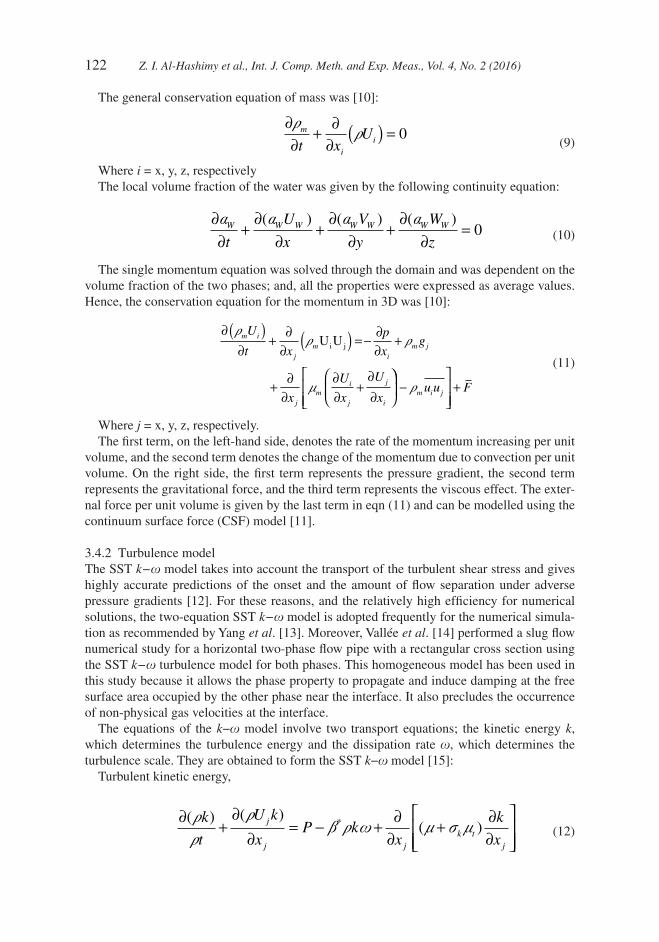
The general conservation equation of mass was [10]:

∂∂

+∂

∂( ) =

rrm

iit x

U 0 (9)

Where i = x, y, z, respectivelyThe local volume fraction of the water was given by the following continuity equation:

∂∂

+∂

∂+

∂∂

+∂

∂=

a a a aW W W W W W W

t

U

x

V

y

W

z

( ) ( ) ( )0 (10)

The single momentum equation was solved through the domain and was dependent on the volume fraction of the two phases; and, all the properties were expressed as average values. Hence, the conservation equation for the momentum in 3D was [10]:

∂( )∂

+∂

∂ ( ) = −∂∂

+

+∂

∂∂∂

+∂∂

rr r

m

m i

jm

im j

jm

i

j

j

i

U

t x

p

xg

x

U

x

U

x

U Ui j

−

+rm i ju u F

(11)

Where j = x, y, z, respectively.The first term, on the left-hand side, denotes the rate of the momentum increasing per unit

volume, and the second term denotes the change of the momentum due to convection per unit volume. On the right side, the first term represents the pressure gradient, the second term represents the gravitational force, and the third term represents the viscous effect. The exter-nal force per unit volume is given by the last term in eqn (11) and can be modelled using the continuum surface force (CSF) model [11].

3.4.2 Turbulence modelThe SST k−w model takes into account the transport of the turbulent shear stress and gives highly accurate predictions of the onset and the amount of flow separation under adverse pressure gradients [12]. For these reasons, and the relatively high efficiency for numerical solutions, the two-equation SST k−w model is adopted frequently for the numerical simula-tion as recommended by Yang et al. [13]. Moreover, Vallée et al. [14] performed a slug flow numerical study for a horizontal two-phase flow pipe with a rectangular cross section using the SST k−w turbulence model for both phases. This homogeneous model has been used in this study because it allows the phase property to propagate and induce damping at the free surface area occupied by the other phase near the interface. It also precludes the occurrence of non-physical gas velocities at the interface.

The equations of the k−w model involve two transport equations; the kinetic energy k, which determines the turbulence energy and the dissipation rate w, which determines the turbulence scale. They are obtained to form the SST k−w model [15]:

Turbulent kinetic energy,

∂

+∂

∂= − +

∂∂

+∂∂

( ) ( )( )*r

rr

b r w m s mk

t

U k

xP k

x

k

xj

j jk t

j

(12)


Specific dissipation Rate,

∂( )∂

+∂( )

∂= − +

∂∂

+( ) ∂∂

+ −

rw r w gn

brw m s m wwt

U

xP

x x

j

j t jt

j

2

2 1 FFk

x xj j1

2( ) ∂∂

∂∂

rsw

ww . .

(13)

Where r is the density of the fluid, k and w are the turbulent kinetic energy and its dissipa-tion frequency, respectively, P is the production of the turbulent kinetic energy, n m rt t= / is the turbulent kinematic viscosity, and m is the molecular dynamic viscosity.

3.5 Implicit integration and time step

Solving complex problems requires the selection of an appropriate numerical method that considers how both accurate and stable the solution is to be. Numerical solutions are either explicit or implicit. Explicit solutions take into account the quantities at the previous time steps to estimate the values of the variables for the current time step. They are usually imple-mented for time-dependent problems in which the time step should be set such that it advances less than one cell distance due to the potential of numerical instabilities. Neighbouring cells have no information about the variables at this stage; as such, it is impractical if the time step jumps to these cells [16]. On the other hand, the implicit method applies iterations through steps to compute the variables based on the known and unknown values at the cells of the current (n) and forward time step (n+1). This method is more computationally intensive but it allows large time steps. In this case, all cells are coupled together so that it is more stable due to its independency of the time step.

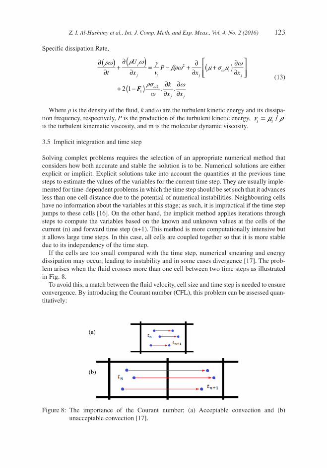
If the cells are too small compared with the time step, numerical smearing and energy dissipation may occur, leading to instability and in some cases divergence [17]. The prob-lem arises when the fluid crosses more than one cell between two time steps as illustrated in Fig. 8.

To avoid this, a match between the fluid velocity, cell size and time step is needed to ensure convergence. By introducing the Courant number (CFL), this problem can be assessed quan-titatively:

Figure 8: The importance of the Courant number; (a) Acceptable convection and (b) unacceptable convection [17].


CFL =∆

∆U t

x (14)

Where U is the fluid velocity, Δt is the time step and Δx is the characteristic cell length. If an implicit solution method is chosen instead of the explicit one, the convergence tends to be more robust. For a quick convergence rate of the solution, Chica [18] suggested that the CFL shall be no more than the unity.

For all cases studied in this work, a transient simulation with a time step of Δt = 0.001 s and cell length of Δx = 0.02 m was identified; such that, the Courant number (CFL) had a value below 1.0 to avoid any instability or numerical diffusion. The entire physical time, t = 7 s, was selected, which was a sufficient time for the slug to be initiated, developed and depart from the exit.

Additionally, a second order temporal discretisation scheme was used for the time domain solution. The High Resolution Interface Capturing scheme (HRIC) was used in this simula-tion to capture the interface between the two phases. The surface tension force based on the CSF was applied in this model to couple the two phases.

4 RESULTS AND DISCUSSION

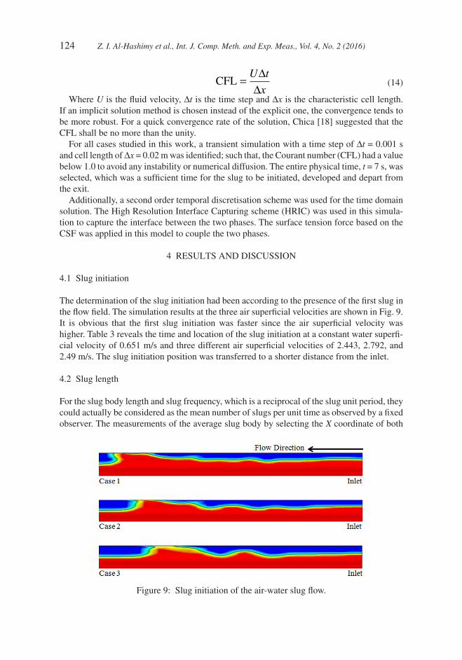
4.1 Slug initiation

The determination of the slug initiation had been according to the presence of the first slug in the flow field. The simulation results at the three air superficial velocities are shown in Fig. 9. It is obvious that the first slug initiation was faster since the air superficial velocity was higher. Table 3 reveals the time and location of the slug initiation at a constant water superfi-cial velocity of 0.651 m/s and three different air superficial velocities of 2.443, 2.792, and 2.49 m/s. The slug initiation position was transferred to a shorter distance from the inlet.

4.2 Slug length

For the slug body length and slug frequency, which is a reciprocal of the slug unit period, they could actually be considered as the mean number of slugs per unit time as observed by a fixed observer. The measurements of the average slug body by selecting the X coordinate of both

Figure 9: Slug initiation of the air-water slug flow.


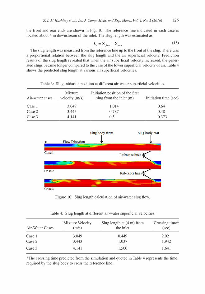
the front and rear ends are shown in Fig. 10. The reference line indicated in each case is located about 4 m downstream of the inlet. The slug length was estimated as

Ls front rear= −Χ Χ (15)

The slug length was measured from the reference line up to the front of the slug. There was a proportional relation between the slug length and the air superficial velocity. Prediction results of the slug length revealed that when the air superficial velocity increased, the gener-ated slugs became longer compared to the case of the lower superficial velocity of air. Table 4 shows the predicted slug length at various air superficial velocities.

Table 3: Slug initiation position at different air-water superficial velocities.

Air-water casesMixture

velocity (m/s)Initiation position of the first

slug from the inlet (m) Initiation time (sec)

Case 1 3.049 1.014 0.64Case 2 3.443 0.787 0.48Case 3 4.141 0.5 0.373

Figure 10: Slug length calculation of air-water slug flow.

Table 4: Slug length at different air-water superficial velocities.

Air-Water CasesMixture Velocity

(m/s)Slug length at (4 m) from

the inletCrossing time*

(sec)

Case 1 3.049 0.449 2.02Case 2 3.443 1.037 1.942

Case 3 4.141 1.500 1.641

*The crossing time predicted from the simulation and quoted in Table 4 represents the time required by the slug body to cross the reference line.


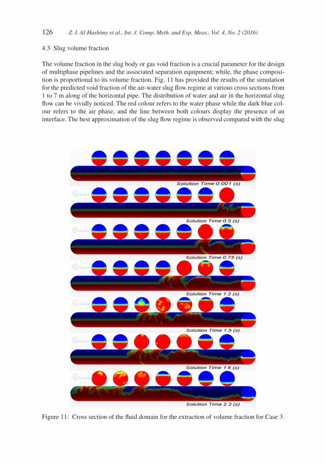
4.3 Slug volume fraction

The volume fraction in the slug body or gas void fraction is a crucial parameter for the design of multiphase pipelines and the associated separation equipment; while, the phase composi-tion is proportional to its volume fraction. Fig. 11 has provided the results of the simulation for the predicted void fraction of the air-water slug flow regime at various cross sections from 1 to 7 m along of the horizontal pipe. The distribution of water and air in the horizontal slug flow can be vividly noticed. The red colour refers to the water phase while the dark blue col-our refers to the air phase, and the line between both colours display the presence of an interface. The best approximation of the slug flow regime is observed compared with the slug

Figure 11: Cross section of the fluid domain for the extraction of volume fraction for Case 3.


flow regime in the Baker char. The water slugs touched the upper part of the pipe and per-formed complete slug regime. As stated before, t = 0 represents the initial conditions where the flow along the pipe was stratified flow, in which the upper part was occupied by air, and the lower part was occupied by water due to the gravitational effect. However, the water phase was steady until the generation of the first wave crest because of the sinusoidal pertur-bation at the inlet; large waves were initiated, which heightened steadily, filling the cross section of the pipe at time 0.5 s.

The long slug was observed at 0.75 s, and it continued to grow along the pipe at the down-stream sections. The tracking for the slug gas void fraction is illustrated in Table 5. Generally, the void fraction increased with the increase in the gas superficial velocity.

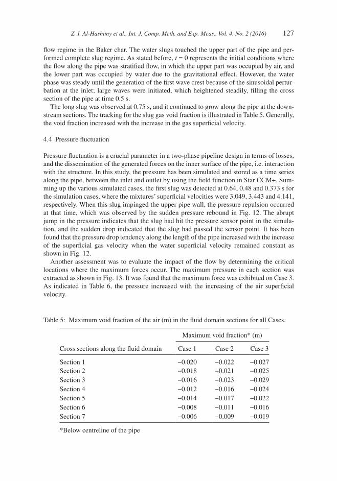
4.4 Pressure fluctuation

Pressure fluctuation is a crucial parameter in a two-phase pipeline design in terms of losses, and the dissemination of the generated forces on the inner surface of the pipe, i.e. interaction with the structure. In this study, the pressure has been simulated and stored as a time series along the pipe, between the inlet and outlet by using the field function in Star CCM+. Sum-ming up the various simulated cases, the first slug was detected at 0.64, 0.48 and 0.373 s for the simulation cases, where the mixtures’ superficial velocities were 3.049, 3.443 and 4.141, respectively. When this slug impinged the upper pipe wall, the pressure repulsion occurred at that time, which was observed by the sudden pressure rebound in Fig. 12. The abrupt jump in the pressure indicates that the slug had hit the pressure sensor point in the simula-tion, and the sudden drop indicated that the slug had passed the sensor point. It has been found that the pressure drop tendency along the length of the pipe increased with the increase of the superficial gas velocity when the water superficial velocity remained constant as shown in Fig. 12.

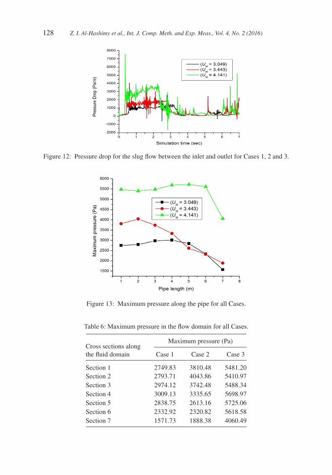
Another assessment was to evaluate the impact of the flow by determining the critical locations where the maximum forces occur. The maximum pressure in each section was extracted as shown in Fig. 13. It was found that the maximum force was exhibited on Case 3. As indicated in Table 6, the pressure increased with the increasing of the air superficial velocity.

Table 5: Maximum void fraction of the air (m) in the fluid domain sections for all Cases.

Cross sections along the fluid domain

Maximum void fraction* (m)

Case 1 Case 2 Case 3

Section 1 −0.020 −0.022 −0.027Section 2 −0.018 −0.021 −0.025Section 3 −0.016 −0.023 −0.029Section 4 −0.012 −0.016 −0.024Section 5 −0.014 −0.017 −0.022Section 6 −0.008 −0.011 −0.016Section 7 −0.006 −0.009 −0.019

*Below centreline of the pipe


Figure 12: Pressure drop for the slug flow between the inlet and outlet for Cases 1, 2 and 3.

Figure 13: Maximum pressure along the pipe for all Cases.

Cross sections along the fluid domain

Maximum pressure (Pa)

Case 1 Case 2 Case 3

Section 1 2749.83 3810.48 5481.20Section 2 2793.71 4043.86 5410.97Section 3 2974.12 3742.48 5488.34Section 4 3009.13 3335.65 5698.97Section 5 2838.75 2613.16 5725.06Section 6 2332.92 2320.82 5618.58Section 7 1571.73 1888.38 4060.49

Table 6: Maximum pressure in the flow domain for all Cases.


5 CONCLUSIONSThis study examined the internal air-water two-phase slug flow behaviour in a horizontal pipe and described the numerical procedure used to simulate the case. Slug initiation and growth was effectively predicted by the 3D transient VOF model combined with the homogeneous k−w turbulence model. The volume fraction profile and pressure variation with time in seven different cross sections along the pipe were examined.

The results of the fluid domain show that:

• As the air superficial velocity increased 2.443, 2.792, and 3.49 m/s, the slug initiation po-sition was transferred closer to the inlet at 0.075DP, 0.058DP, and 0.037DP, respectively.

• It was further observed that as the air superficial velocity increased 2.443, 2.792, and 3.49 m/s, the slug length increased to 0.033 DP, 0.077 DP and 0.11 DP.

• The void fraction was increased as the air superficial increased.

• The pressure drop tendency along the length of the pipe increased with the increase of the gas superficial velocity when the water superficial velocity remained constant.

It is recommended, for the future work, to experimentally investigate the mentioned cases of slug flow to validate the present numerical outcomes and, to clearly correlate the slug flow-induced vibration in the structure to the slug characteristics.

ACKNOWLEDGEMENTThe authors acknowledge Universiti Teknologi PETRONAS (UTP) for the financial support to carry out the research. The main author expresses his appreciation to UTP for sponsoring his PhD study under the Graduate Assistance scheme (GA).

REFERENCES [1] Ghorai, S. & Nigam, K.D.P., CFD modeling of flow profiles and interfacial phenomena

in two-phase flow in pipes. Chemical Engineering and Processing: Process Intensifica-tion, 45(1), pp. 55–65, 2006.http://dx.doi.org/10.1016/j.cep.2005.05.006

[2] Brennen, C.E., Fundamentals of Multiphase Flow, Cambridge University Press: New York, 2005.http://dx.doi.org/10.1017/CBO9780511807169

[3] Hill, T.J., Fairhurst, C.P., Nelson, C.J., Becerra, H. & Bailey, R.S., Multiphase Pro-duction through Hilly Terrain Pipelines in Cusiana Oilfield Colombia. SPE Annual Technical Conference and Exhibition. Society of Petroleum Engineers, 1996.http://dx.doi.org/10.2118/36606-MS

[4] Orell, A., Experimental validation of a simple model for gas–liquid slug flow in horizontal pipes. Chemical Engineering Science, 60(5), pp. 1371–1381, 2005.http://dx.doi.org/10.1016/j.ces.2004.09.082

[5] Baker, O., Simultaneous flow of oil and gas. Oil and Gas Journal. 53, pp. 185–195, 1954.

[6] Rashimi, W., Choong, T.S.Y., Chuah, T.G., Aslina, S. & Khalid, M., Effect of interphase forces on two-phase liquid- liquid flow in horizontal pipe. Journal - The Institution of Engineers, Malaysia, 71(2), pp 35–40, 2010.

[7] Al-Hashimy, Z.I., Al-Kayiem, H.H., Kadhim, Z.K. & Mohmmed, A.O., Numerical sim-ulation and pressure drop prediction of slug flow in oil/gas pipelines. WIT Transactions on Engineering Sciences, 89, 2015, ISSN 1743-3533.


[8] Wongwises, S., Khanhaew, W. & Vetchsupakhun, W., Prediction of liquid holdup in horizontal stratified two-phase flow. Thammasat International Journal of Science and Technology, 3(2), pp. 48–56, 1998.

[9] Ranade, VV., Computational Flow Modeling for Chemical Reactor Engineering, Vol. 5. Academic press, 2001.

[10] Iacovides, H., Kelemenis, G. & Raisee, M., Flow and heat transfer in straight cooling passages with inclined ribs on opposite walls: an experimental and computational study. Experimental Thermal and Fluid Science, 27(3), pp. 283–294, 2003.

[11] Brackbill, J.U., Kothe, D.B. & Zemach, C., A continuum method for modeling surface tension. Journal of Computational Physics, 100(2), pp. 335–354, 1992.http://dx.doi.org/10.1016/0021-9991(92)90240-Y

[12] Menter F.R., Two-equation eddy-viscosity turbulence models for engineering applica-tions. AIAA Journal, 32(8), pp. 1598–1605, 1994.http://dx.doi.org/10.2514/3.12149

[13] Yang, Yi., Ming G. & Xinyang J., New inflow boundary conditions for modeling the neutral equilibrium atmospheric boundary layer in SST k-w model. Proceedings of the Seventh Asia Pacific Conference on Wind Engineering, Taipei, Taiwan, November 8–12, 2009.

[14] Vallée, C., Höhne, T., Prasser, HM. & Sühnel T., Experimental investigation and CFD simulation of horizontal stratified two-phase flow phenomena. Nuclear Engineering and Design, 238(3), pp. 637–646, 2008.http://dx.doi.org/10.1016/j.nucengdes.2007.02.051

[15] Wilcox, D.C., Turbulence Modeling for CFD, DCW Industries Inc: La Canada, Cali-fornia, 2006.

[16] Science Flow, Flow-3D, available at http://www.flow3d.com/cfd-101/cfd-101-implicit-explicit-schemes.html, 2013 (accessed 20 October 2013).

[17] Aagaard, O., Hydroelastic analysis of flexible wedges. PhD thesis, Norwegian Univer-sity of Science and Technology, 2013.

[18] Chica, L., FSI study of internal multiphase flow in subsea piping components. PhD diss, University of Houston, 2014.

numerical characterisation of slug flow in horizontal … · horizontal air /water pipe flow ......

Documents