The Astrophysical Journal, 737:21 (14pp), 2011 August 10 doi:10.1088/0004-637X/737/1/21C© 2011. The American Astronomical Society. All rights reserved. Printed in the U.S.A.

NUMERICAL CALCULATION OF MAGNETOBREMSSTRAHLUNG EMISSION ANDABSORPTION COEFFICIENTS

Po Kin Leung1, Charles F. Gammie

2,3, and Scott C. Noble

41 Department of Physics, University of California, Santa Barbara, CA 93106, USA; pkleung@physics.ucsb.edu

2 Astronomy Department, University of Illinois, Urbana, IL 61801, USA3 Physics Department, University of Illinois, Urbana, IL 61801, USA; gammie@illinois.edu

4 Center for Computational Relativity and Gravitation, School of Mathematical Sciences, Rochester Institute of Technology,Rochester, NY 14623, USA; scn@astro.rit.edu

Received 2009 October 29; accepted 2011 May 13; published 2011 July 26

ABSTRACT

Magnetobremsstrahlung (MBS) emission and absorption play a role in many astronomical systems. We describea general numerical scheme for evaluating MBS emission and absorption coefficients for both polarized andunpolarized light in a plasma with a general distribution function. Along the way we provide an accurate schemefor evaluating Bessel functions of high order. We use our scheme to evaluate the accuracy of earlier fitting formulaeand approximations. We also provide an accurate fitting formula for mildly relativistic (kT /(mec

2) � 0.5) thermalelectron emission (and therefore absorption). Our scheme is too slow, at present, for direct use in radiative transfercalculations but will be useful for anyone seeking to fit emission or absorption coefficients in a particular regime.

Key words: methods: numerical – radiation mechanisms: general

Online-only material: color figures

1. INTRODUCTION

In many astronomical plasmas the electron distribution in-cludes an approximately thermal, mildly relativistic compo-nent. As theoretical models of such systems advance, it isuseful to have a fast, accurate scheme to calculate the mag-netobremsstrahlung (MBS), or cyclo-synchrotron, spectra. It isparticularly desirable to be able to evaluate the necessary ab-sorption and emission coefficients for polarized radiation froma general electron distribution, since in the collisionless condi-tions common in low luminosity active galactic nuclei electrondistributions are unlikely to precisely follow the commonly as-sumed thermal or power-law forms.

Usually MBS spectra are calculated using emission and ab-sorption coefficients derived under an ultrarelativistic (syn-chrotron) approximation or, for mildly relativistic electrons,using approximate fitting formulae. The fitting formulae areaccurate over a limited range in frequency ν, field strength B,observer angle θ (the angle between the emitted or absorbed pho-ton and the magnetic field vector B), or characteristic Lorentzfactor for the electrons. In this work we provide, test, and applya general scheme for calculating MBS emission and absorptioncoefficients. One potential application of our methods is to gen-erate new, more accurate, and computationally efficient fittingformulae over the range of interest.

Approximate calculations of MBS emission and absorptioncoefficients have a rich history. In the ultrarelativistic limit,emission of an electron with Lorentz factor γ is limited to acone defined by the oscillating velocity vector of the electron,with angular width 1/γ . This leads to an approximate expressionfor dP/dν (Westfold 1959; Bekefi 1966; Rybicki & Lightman1979), the power per unit frequency interval. However, forγ ∼ 1, the approximation worsens, cyclotron line features beginto appear in the spectrum, and the ultrarelativistic approximationmust be abandoned.

For mildly relativistic electrons the emission is still mainlyperpendicular to the magnetic field. This fact can be used todevelop approximate analytic expressions for the emissivity.

Petrosian (1981) used the method of steepest descent, andan asymptotic expansion of the Bessel functions, to find theemissivity of mildly relativistic thermal electrons (see alsoPacholczyk 1970).

Robinson & Melrose (1984) and Dulk (1985) improvedPetrosian’s (1981) calculation for thermal electrons at temper-ature T by using more accurate asymptotic expansions of theBessel functions that appear in the exact expression for theemissivity, and some interpolation formulae, to provide a ther-mal MBS emissivity that is valid over a wide range in T , ν, θ,and B. Brainerd & Lamb (1987) numerically calculate emis-sivity for various distributions and energy injection functions.Brainerd & Petrosian (1987) calculate emissivity in the regimethat quantum effects are important. Chanmugam et al. (1989)compared several approximate equations with numerical resultsin the cyclotron limit and concluded that Robinson & Melrose(1984) gave the best result. Mahadevan et al. (1996) found ap-proximate formulae for the θ -averaged emission coefficient byfitting to a direct numerical evaluation of the emissivity.

Wardzinski & Zdziarski (2000) combined the approximateequations in Petrosian (1981) and Petrosian & McTiernan(1983) to find an approximate emissivity accurate over alarger range of temperature. Their expressions contain a slightdiscontinuity, however, because they joined two asymptoticlimits without smoothing the intermediate regime. They alsofound an approximate θ -averaged emissivity.

For polarized light, Kawabata (1964) and Meggitt &Wickramasinghe (1982) gave complicated but exact integral ex-pressions for the specific emissivities in the Stokes formalism,but they did not provide any easily evaluated approximations.Vath & Chanmugam (1995) used the results of Robinson & Mel-rose (1984) to obtain the approximate equations and comparedthe results with a direct numerical evaluation of the emissivityin the cyclotron regime.

We began this work because, in attempting to calculate polar-ized emission spectra for our simulation, we found we neededto evaluate the accuracy of earlier approximate expressions inthe regime of interest to us. Here we provide what we hope is a

1

The Astrophysical Journal, 737:21 (14pp), 2011 August 10 Leung, Gammie, & Noble

transparent, well-documented procedure that will enable othersto avoid our descent into the minutiae of synchrotron theory.Our MBS calculator has a broad range of validity (described inSection 4) and should therefore be useful for anyone seekingto obtain or test approximate expressions in their domain ofinterest.

The main approximations we make are (1) (ν/νp)2 � 1 and(2) (ν/νp)2(ν/νc) � 1, where the electron plasma frequency

νp ≡(

nee2

πme

)1/2

= 8980n1/2e Hz (1)

(we use Gaussian/cgs units throughout) and the electron cy-clotron frequency

νc ≡ eB

2πmec= 2.8 × 106B Hz. (2)

When these conditions are violated the index of refractionis noticeably different from 1 and corrections must be madethroughout our formalism. We also assume that the magneticfield strength is weak enough such that quantum effects can beneglected (see discussion in Brainerd & Lamb 1987 for details).

The plan of this paper is as follows. In Section 2, we fixnotation by writing down the equations of polarized radiativetransfer in Stokes and Cartesian polarization bases. In Section 3,we discuss methods for calculating the emission and absorptioncoefficients for a general distribution function. In Section 4,we recall the usual asymptotic expressions that can be used ascode checks. In Section 5, we describe our numerical code,called harmony. In Section 6, we evaluate the accuracy ofearlier work and provide a convenient fitting formula for thetotal emissivity (and therefore absorptivity) of thermal electronswith Θe ≡ kTe/(mec

2) � 0.5. Appendix A briefly describes thedistinction between emitted and received power. Appendix Bdescribes an accurate and efficient scheme for evaluating high-order Bessel functions.

2. RADIATIVE TRANSFER

We are concerned with electromagnetic wave propagationat frequency ν in the frame of a magnetized, ionized plasma.The plasma may have a thermal electron component withdimensionless temperature Θe; there may also be a nonthermalcomponent in the electron distribution.

In the regime of interest an electromagnetic wave can bewritten as a sum of the magnetoionic modes of the plasma, theordinary (O) and extraordinary (X) modes. In the simplest caseof a cold plasma, for which the thermal speed is much less thanthe phase velocities of waves in the plasma, these modes arenearly circularly polarized except for propagation in a narrowrange of angles perpendicular to the field. In general the modesare elliptically polarized.

The polarization properties of the magnetoionic modes aredescribed by a pair of orthonormal basis vectors eO andeX, which can be written in terms of unit vectors along thewavevector k, along k × B, and perpendicular to both k andB. Let TO (TX) be the ratio of coefficients along the twotransverse components of the polarization vector of the ordinary(extraordinary) mode, with |TX| � 1. In other words, |TO,X| arethe axial ratios of the orthogonal polarization ellipses, so thatTOTX = −1. Then

eO ≡ {eO1, eO2} = 1√T 2

X + 1{−1, iTX} (3)

and

eX ≡ {eX1, eX2} = 1√T 2

X + 1{TX, i} , (4)

where {x, y} are the Cartesian components of a vector in theplane perpendicular to the direction of propagation z, and yis perpendicular to the magnetic field so that x × y ≡ z. Theelectric field of mode A is E = EeA exp(ikz − iωt). In writingthese equations we have assumed that the polarization modesare orthogonal, valid when ν3/(νp

2νc) � 1.

2.1. Descriptions of Polarized Radiation

The polarized intensity is most familiarly described by theStokes vector IS = {I,Q,U, V }; here, all components have theusual intensity units, dE/dtd2xdνdΩ, i.e., energy per unit timeper unit area per unit frequency per unit solid angle.

The polarized intensity can also be described in terms of apolarization tensor written in a Cartesian coordinate basis (∗denotes complex conjugate):

Iij ≡ I

E2〈EiE

∗j 〉 = 1

2

(I + Q U + iV

U − iV I − Q

), (5)

where i, j ∈ {x, y} and the prefactor converts the tensor tointensity units.

Finally, the polarized intensity can be described by a polar-ization tensor in the mode basis

IAB = e∗AieBj Iij

= 1

2

(I − Q cos χ − V sin χ −V cos χ + Q sin χ − iU

−V cos χ + Q sin χ + iU I + Q cos χ + V sin χ

)(6)

where A,B ∈ {O,X} and χ = tan−1 TX.

2.2. Polarized Radiative Transfer

In the Stokes basis in a uniform plasma the radiative transferequation is

d

dsIS = JS − MST IT , (7)

where JS = {jI , jQ, jU , jV }T contains the emission coefficients,which have units of dE/dtdV dνdΩ, and the Mueller matrixMST is

MST ≡

⎛⎜⎝

αI αQ αU αV

αQ αI rV −rU

αU −rV αI rQ

αV rU −rQ αI

⎞⎟⎠ . (8)

The parameters αi are the absorption coefficients and rQ, rU ,and rV are what we will call Faraday mixing coefficients. jU , αU ,and rU are zeros for our choice of basis vectors. Below, we willprovide a scheme for evaluating the emission and absorptioncoefficients.

In the Cartesian polarization tensor basis in a uniform plasmathe transfer equation is

dIij

ds= Jij − μijklIkl, (9)

where the tensor μ describes absorption and Faraday rotation.In the mode basis in a uniform plasma

dIAB

ds= JAB − μABCDICD. (10)

2

The Astrophysical Journal, 737:21 (14pp), 2011 August 10 Leung, Gammie, & Noble

Contracting the indices, we define αA by

dIAA

ds= −αAIAA, (11)

for radiation consisting of a single mode in the absence ofemission and Faraday rotation.

3. MAGNETOBREMSSTRAHLUNG EMISSIONAND ABSORPTION

We are now ready to calculate absorption and emissioncoefficients. These are frame-dependent. We will evaluate themin the plasma center-of-momentum frame (the expressions givenbelow do not assume this). The total emission and absorptioncoefficients can be transformed using the Lorentz invariance ofjν/ν

2 and ναν . The transformation of the full absorption matrixwill be discussed in future work.

3.1. Emissivity

A consistent procedure for calculating the emission and ab-sorption coefficients can be found in Melrose & McPhedran(1991). Beginning with their Equation (22.20), rotating the ve-locity potentials Vi onto a basis where the z-direction is alignedwith the wavevector, and introducing appropriate leading con-stants, the emissivity in the Cartesian polarization basis is

Jij = 2πe2ν2

c

∫d3p f

∞∑n=1

δ(yn) Kij (12)

whereKxx = M2J 2

n (z), (13)

Kyy = N2J ′2n (z), (14)

Kxy = −Kyx = −iMNJn(z)J ′n(z), (15)

and

yn ≡ nνc

γ−ν(1−β cos ξ cos θ ) = 1

2π(ω−nΩ−k‖v‖) (16)

is the argument of the δ function in the resonance condition,Ω = 2πνc/γ is the relativistic electron cyclotron angularfrequency, β ≡ v/c, v is the electron speed, ξ is the electronpitch angle,

z ≡ νγβ sin θ sin ξ

νc= k⊥v⊥

Ω, (17)

M ≡ cos θ − β cos ξ

sin θ, (18)

N ≡ β sin ξ, (19)

f ≡ dNe

d3xd3p= dne

d3p(20)

is the electron distribution function, and d3x and d3p are differ-ential volumes in real space and momentum space, respectively.Subscripts ‖ and ⊥ refer to components of vectors parallel andperpendicular to B.

The emissivity in the Stokes basis can be found using thetransformation implied by Equation (5):

JS = 2πe2ν2

c

∫d3p f

∞∑n=1

δ(yn)KS (21)

whereKI = M2J 2

n (z) + N2J ′2n (z), (22)

KQ = M2J 2n (z) − N2J ′2

n (z), (23)

KU = 0, (24)

andKV = −2MNJn(z)J ′

n(z). (25)

In the mode basis

JAB = 2πe2ν2

c

∫d3p f

∞∑n=1

δ(yn)KAB (26)

where

KXX = [MTXJn(z) + NJ ′n(z)]2

1 + T 2X

, (27)

KOO = [MJn(z) − NTXJ ′n(z)]2

1 + T 2X

, (28)

and

KXO = KOX = − [MJn(z) − NT J ′n(z)][MT Jn(z) + NJ ′

n(z)]

1 + T 2X

.

(29)In the cold plasma limit, the axial ratios are (e.g., Melrose 1989)

TO,X ≡ T± ≈ 2ν cos θ

νc sin2 θ ∓√

νc2 sin4 θ + 4ν2 cos2 θ

for ν � νp.

(30)

The polarized emissivities are related to the total emissivityby

jν ≡ JI = Jxx + Jyy = JOO + JXX ≡∫

d3pf ην, (31)

where

ην ≡ dE

dνdtdΩ(32)

is the single-electron emissivity.

3.2. Absorption Coefficients

If the distribution function is thermal then the absorptioncoefficients follow from Kirchhoff’s law. For a nonthermalplasma we must calculate the absorption coefficients directly.

If the plasma is weakly anisotropic (i.e., the anisotropic effectis perturbative) then it is possible to simply relate the absorptioncoefficients to the anisotropic, antihermitian part of the dielectrictensor. Starting with the dielectric tensor of a magnetized plasma(Equation (22.47) of Melrose & McPhedran 1991, corrected bya factor of 4π/ω2, or Equations (10)–(48) of Stix 1992), andusing the Plemelj relation to find the imaginary part of the

3

The Astrophysical Journal, 737:21 (14pp), 2011 August 10 Leung, Gammie, & Noble

integral over momentum space (and thus the antihermitian partof the dielectric tensor), we find

μijkl = ce2

ν

∫d3p Df

∞∑n=1

δ(yn)Kijkl, (33)

whereKxxxx = M2J 2

n (z), (34)

Kxxyx = Kxyxx = Kxyyy = Kyyyx = − i

2MNJn(z)J ′

n(z),

(35)

Kxxxy = Kyxxx = Kyxyy = Kyyxy = i

2MNJn(z)J ′

n(z), (36)

Kxyxy = Kyxyx = 1

2

[M2J 2

n (z) + N2J ′2n (z)

], (37)

Kyyyy = N2J ′2n (z), (38)

all other components of K vanish, and the operator D is

Df ≡(

ω − k‖v‖v⊥

∂

∂p⊥+ k‖

∂

∂p‖

)f. (39)

In writing this equation, we assume that the energy of the ab-sorbed photon is small compared to the width of the distributionfunction, permitting us to replace a difference with the deriva-tive operator D. For a thermal distribution this requires thathν/kTe � 1.

In terms of p = |p| and cos ξ , the operator D is

Df = 2πν

cβ

(∂

∂p+

β cos θ − cos ξ

p

∂

∂ cos ξ

)f, (40)

and in terms of γ and cos ξ ,

Df = 2πν

(1

mec2

∂

∂γ+

β cos θ − cos ξ

pβc

∂

∂ cos ξ

)f. (41)

In the Stokes basis,

αS = −ce2

2ν

∫d3p

∞∑n=1

δ(yn)Df KS, (42)

where subscript S is one of I, Q, U, and V. In the mode basis

αA = −ce2

ν

∫d3p

∞∑n=1

δ(yn)Df KAA, (43)

where subscript A is O or X.Let us explicitly verify Kirchhoff’s law for a thermal distri-

bution function in the Stokes basis:

JS − αSBν = 0, (44)

where Bν = (2hν3/c2)[exp(hν/kTe) − 1]−1 is the Planckfunction. Using Equations (21) and (42), and gathering liketerms, this becomes

∫d3p

∞∑n=1

δ(yn)KS

(2πe2ν2

cf +

ce2

2νDf Bν

)= 0. (45)

If we make γ the nontrivial momentum space coordinate, thenf = N exp(−γ /Θe), where N (Θe) is a normalization constant,and Df = −2πNν exp(−γ /Θe)/(mec

2Θe). This leaves

∫d3p

∞∑n=1

δ(yn)KS

(2πe2ν2

c

)Ne−γ /Θe

×(

1 − hν/(kTe)

exp(hν/(kTe)) − 1

)= O

(hν

kTe

). (46)

This is consistent with the assumption that the energy ofthe absorbed photon is small compared to the width of thedistribution function; to lowest order in hν/kTe Kirchhoff’s lawis satisfied.

3.3. Electron Distribution Function

The electron distribution can be written using a variety ofmomentum space coordinates, and this can be a source of someconfusion. For example, with respect to the auxiliary momentumcoordinates γ , ξ, and φ (the longitudinal coordinate), d3p canbe expressed as m3

ec3γ 2βdγ d(cos ξ )dφ and the distribution

function as

f ≡ dne

d3p= 1

m3ec

3γ 2β

dne

dγ d(cos ξ ) dφ

= 1

2πm3ec

3γ 2β

dne

dγ d(cos ξ ), (47)

where the final equality arises from assuming that the distribu-tion is independent of φ. Equation (42) becomes

αS = −ce2

2ν

∫dγ d(cos ξ )

∞∑n=1

δ(yn)γ 2βD

×[

1

γ 2β

dne

dγ d(cos ξ )

]KS (48)

and similarly for the absorption coefficients in the mode basis.The thermal (relativistic Maxwellian) distribution function is

dne

dγ dΩp

≡ dne

dγ dφd(cos ξ )= ne

4πΘe

γ (γ 2 − 1)1/2

K2(1/Θe)exp

(− γ

Θe

);

(49)dΩp is a differential solid angle in momentum space and K2 isa modified Bessel function of the second kind.

A useful nonthermal distribution function is the isotropicpower-law distribution

dne

dγ dΩp

= nNTe (p − 1)

4π(γ

1−pmin − γ

1−pmax

)γ −p for γmin � γ � γmax,

(50)where nNT

e is the number density of nonthermal electrons.

4. ULTRARELATIVISTIC LIMIT

For clarity it is helpful to record the emission and absorptioncoefficients for a thermal electron distribution and for a power-law distribution of electrons in the ultrarelativistic limit. Theseare well known but presented here in a consistent set of unitsand notation so that we can check our numerical results.

The emissivity of a single ultrarelativistic electron can bereduced through a standard approximation (e.g., Westfold 1959;

4

The Astrophysical Journal, 737:21 (14pp), 2011 August 10 Leung, Gammie, & Noble

Ginzburg 1970)

∫dΩpην �

√3e3B sin θ

mec2F

(ν

νcr

), (51)

where νcr = (3/2)νc sin θγ 2, and the synchrotron function

F (x) ≡ x

∫ ∞

x

dtK5/3(t). (52)

The asymptotic expansions of F (x) are

F (x) =⎧⎨⎩

22/3Γ(2/3)x1/3 + O(x) for x � 1(πx

2

)1/2exp(−x)(1 + O(x−1)) for x � 1

⎫⎬⎭ .

(53)For a thermal distribution with Θe � 1, K2(1/Θe) � 2Θ2

e

anddne

dγ dΩp

� neγ2

8πΘ3e

exp(−γ /Θe). (54)

For ν � νs ≡ (2/9)νcΘ2e sin θ , the small-x limit of Equation (53)

can be used, most of the emission comes from electrons withγ ∼ Θe, and the emissivity is

jν � 24/3π

3

nee2νs

cΘ2e

X1/3, (55)

whereX ≡ ν

νs. (56)

For ν � νs the large-x limit of Equation (53) applies.The integrand is proportional to exp(−γ /Θe − ν/νcr), whereνcr ∼ γ 2, so the peak emission is from electrons with γ ∼(νΘe/(νc sin θ ))1/3. Then,

jν � ne

√2πe2νs

6Θ2ec

X exp(−X1/3), (57)

and the integral has been evaluated using the method of steepestdescent (Petrosian 1981).

For the isotropic power-law distribution of electrons theintegration can be done explicitly without using the asymptoticexpansion for F (x) if p > 1. Most of the emission comes fromelectrons with γ 2 ∼ ν/νc, and the emissivity is (Blumenthal &Gould 1970)

jν = nNTe

(e2νc

c

)3p/2(p − 1) sin θ

2(p + 1)(γ

1−pmin − γ

1−pmax

)Γ(

3p − 1

12

)

× Γ(

3p + 19

12

) (ν

νc sin θ

)−(p−1)/2

(58)

for γ 2min � ν/νc � γ 2

max. The absorptivity, famously, cannotbe obtained from Kirchhoff’s law, but can be evaluated usingEquation (42). The result is (see, e.g., Rybicki & Lightman 1979for a discussion)

αν = nNTe

(e2

νmec

)3(p+1)/2(p − 1)

4(γ

1−pmin − γ

1−pmax

)Γ(

3p + 2

12

)

× Γ(

3p + 22

12

)(ν

νc sin θ

)−(p+2)/2

, (59)

again for γ 2min � ν/νc � γ 2

max. Note that this expressionfor the absorptivity is proportional to nNT

e e2/(νmec). Since(nNT

e e2/me)1/2 is a plasma frequency for the nonthermal elec-trons, the absorption coefficient has the expected dimensions of1/length.

5. NUMERICAL CALCULATIONS

The emission and absorption coefficients all require thenumerical evaluation of expressions of the following form:

∫ ∞

1dγ

∫ 1

−1d cos ξ

∞∑n=1

δ(yn)I (n, ξ, γ ), (60)

where I is some function, ξ is the electron pitch angle, γ is theelectron Lorentz factor, and n is the harmonic index (see, e.g.,Equation (21)), and the resonance condition is

yn ≡ nνc

γ− ν(1 − β cos ξ cos θ ) = 0, (61)

which involves all three independent variables: γ, ξ, and n.Recall that the resonance condition arises because each electronemits only at integer multiples of its own cyclotron frequency,Doppler shifted to the plasma rest frame.

5.1. Previous Work

Many have evaluated the absorption and emission coefficientsnumerically. Early efforts include the calculation of jν(θ ) byTakahara & Tsuruta (1982) for n up to several hundred. Melia(1994) calculated the emissivity numerically for θ = π/2.

The emissivity is sharply peaked at particular ν; the inte-grand is not well behaved. Mahadevan et al. (1996) resolvedthe resulting numerical difficulty by replacing the δ functionwith a broadening function of adjustable frequency width andevaluating the full three-dimensional integral. Only an observerangle-averaged emission coefficient, jν ≡ ∫ 1

0 jν(θ )d(cos θ ),was found. The resonance condition was also used to simplifythe integral.

Marcowith & Malzac (2003) found the angle-averaged emis-sion coefficient by two methods. The first was similar toMahadevan et al. (1996) except that a different broadening func-tion was used. Another method, “direct integration,” used theresonance condition to select an observer angle.

Wolfe & Melia (2006) calculated the angle-averaged single-particle emissivity and extended the summation to the 990thharmonic to increase the accuracy of the result. The calculationwas done by replacing the δ function with a broadeningfunction, as in Mahadevan et al. (1996). The single-particleemissivity was then fitted with >1500 coefficients over the range−1 < log10(ν/νc) < 2 and 0.1 < β < 0.98. For the thermalemissivity, they explicitly evaluated the γ integral for β < 0.97;for β > 0.97 they used an approximation from Petrosian (1981).They restricted their calculation to −1 < log10(ν/νc) < 2; theydid not offer an explicit control for the accuracy of the n � 990approximation for a particular γ .

5.2. Numerical Procedure

We use the resonance condition (61) to eliminate cos ξ fromEquation (60). This is simpler than eliminating γ (because theresonance condition is quadratic in β), and also simpler than

5

The Astrophysical Journal, 737:21 (14pp), 2011 August 10 Leung, Gammie, & Noble

eliminating n (because n must take on integer values). Theremaining integral has the form∫ γ+

γ−dγ

∞∑n=n−

(1

νβ|cos θ |)

I (n, ξ, γ ) (62)

and the term in parentheses, |dyn/d cos ξ |−1, comes fromintegrating over the δ function. The range of integration is nowrestricted by the requirements that |cos ξ | < 1 and that γ bereal.

The limits on the γ integration follow from |cos ξ | < 1. Writethe resonance condition

cos ξ = γ ν − nνc

γ νβ cos θ, (63)

and set cos ξ = ±1 to find

γ± = nνc/ν ± |cos θ |√

(nνc/ν)2 − sin2 θ

sin2 θ. (64)

Note that γ− reaches a minimum of 1 for nνc/ν = 1, so γ− � 1.The argument of the square root in Equation (64) must be

non-negative. This restricts the range of n to

n � n− = ν

νc|sin θ |. (65)

At n−, γ+ = γ−.We need to choose an order to evaluate the integrals (sums)

in Equation (62). If the sum is done first then the remainingintegrand is a rapidly varying, comb-like, function of γ for θclose to π/2. If the γ integration is done first the remaining sum-mand is a smooth function of n and therefore more numericallytractable. We therefore do the γ integration first.

5.3. Upper Limit of Summation

The summation in Equation (62) extends to n = ∞, so fornumerical summation we must either map n onto a finite domainor else choose an upper limit n+ to the sum, beyond which theintegrand is negligible. We have taken the latter approach.

For the special case of a thermal electron distribution we setn+ = Cnpeak, where the integrand peaks near npeak and C > 1is a dimensionless constant. At ν � νcΘ2

e , the integrand peakswhen Jn(z) peaks, at z/n � 1, i.e., near

n = npeak = γν

νc(1 − β2 cos2 θ ). (66)

The thermal distribution is proportional to exp(−γ /Θe)/K2(1/Θe). This peaks at γ ∼ 1 + Θe for all Θe, so

npeak � (Θe + 1)(ν/νc)(1 − β2 cos2 θ ) (67)

is a good estimate for all Θe.For ν � νcΘ2

e we can use the asymptotic expression for thesingle electron emissivity to estimate npeak (see Section 5). Thepeak is near the peak of the function exp[−γ /Θe − ν/(γ 2νc)],so most of the emission comes from electrons with γ =(2Θeν/νc)1/3.

Combining the low-frequency and high-frequency estimatesfor npeak,

n+ = C

[Θe + 1 +

(2Θe

ν

νc

)1/3]

ν

νc(1 − β2 cos2 θ ). (68)

Typically C = 10 gives adequate accuracy.For a nonthermal distribution we take an adaptive approach.

We sum over successive intervals [n−, n− + Δn], [n− + Δn +1, 2(n− + Δn)], [2(n− + Δn) + 1, 4(n− + Δn)], etc., until thefractional contribution from the last interval is smaller than apreset tolerance. This procedure yields fast convergence exceptfor exotic electron distribution functions. Some knowledge ofthe distribution is required, however, to set Δn.

5.4. Numerical Considerations

Accurate, efficient evaluation of the Bessel function Jn(z) forn � 1 is essential for our calculation. When n is small, anymathematical library gives an accurate, efficient result. As nincreases, however, standard mathematical libraries slow down,become inaccurate, and fail. In our calculations, the argument zand order n of the Bessel functions can be large and are typicallycomparable in size (one can show that z/n < 1). Standardasymptotic expansions (see Abramowitz & Stegun 1970) areunsatisfactory because they typically assume z � n or viceversa. We calculate Jn using a special-purpose code based onasymptotic expansions discussed in Chishtie et al. (2005), whodivide the arguments into three regimes and provide asymptoticexpansions for each regime. Details of our scheme are discussedin Appendix B.

The summation over n is done as an explicit sum at smalln and as an integral at large n. The same approach wasused by Takahara & Tsuruta (1982). Approximating the sumas an integral at large n increases both speed and, in manycases, accuracy. The breakpoint, nI , between summation andintegration is set heuristically. Typically, we use nI = 30 for theparameters of interest to us.

We integrate using the GNU Scientific Library’s QAG inte-grator, which is fast, robust, and publicly available. One subtletyhere is connected to the narrow extent of the γ integrand whenν is large (this narrow extent permits one to use the methodof steepest descent in evaluating Equation (57)). If the domainof integration is not set correctly then the integrator can failto resolve the peak and the emissivity, for example, will beunderestimated.

Finally, note that Equation (62) fails for θ = π/2 becausethe δ function does not contain cos ξ and so cannot be used toeliminate the cos ξ integral. But since jν(θ ) is a smooth functionof θ with a maximum at θ = π/2, we simply avoid evaluatingthe emissivity at θ = π/2 by extrapolating from nearby θ . Theerror is of the same order as a single integration because of thezero slope around the peak. The only penalty is that the timeneeded to find jν is doubled compared to the calculation at otherθ .

6. VERIFICATION OF CALCULATION

6.1. Monoenergetic Electrons

The angle-averaged synchrotron emissivity of ultrarelativisticmonoenergetic electrons is

jν(ν, γ ) � ne

1

2

∫ 1

−1

√3e3B sin θ

4πmec2F

(ν

νcr

)d(cos θ ) ≡ neην.

(69)The single-particle emissivity can be approximated as (Crusius& Schlickeiser 1986, 1988; Schlickeiser & Lerche 2007)

ην(ν, γ ) ≈ πe2ν

2√

3cγ 2CS

[2ν

3νcγ 2

], (70)

6

The Astrophysical Journal, 737:21 (14pp), 2011 August 10 Leung, Gammie, & Noble

Figure 1. Upper panel: the angle-averaged single-particle emissivity ην/B, incgs units, at β = 0.999. The solid line is the result of harmony, and the dashedline is calculated by using the approximate Equation (70). Lower panel: the solidline is the relative difference of Equation (70) and the result of harmony, andthe dotted line is the difference between Equation (70) and the ultrarelativisticlimit Equation (69).

Figure 2. Upper panel: the angle-averaged single-particle emissivity ην/B, incgs units, at β = 0.86. The solid line is result of harmony, and the dashed lineis result of Wolfe & Melia (2006) multiplied by a factor of π2 (which we cannotexplain). Lower panel: the relative difference of ην . The difference comparedto Wolfe & Melia (2006, their Figure 3) seems to be due to better resolution ofthe cyclotron peaks in our calculation.

where the function CS(x) is given by

CS(x) = x−2/3

0.869 + x1/3 exp(x). (71)

We compute an approximation to the emissivity of a monoen-ergetic distribution by using a narrow Gaussian in energy; forsmall enough energy width ΔE the emissivity is independent ofΔE. Figure 1 compares Equation (70) with the harmony resultand the ultrarelativistic limit Equation (69). At high frequency,harmony underestimates the emissivity because the integrandbecomes too narrow to be resolved numerically. Evidently,Equation (71) has a maximum error of order ≈20%.

Wolfe & Melia (2006) fit the angle-averaged single-particleemissivity and provide a code that reproduces their fittingfunction. Figure 2 compares results of harmony with their code,with the same parameters as their Figure 3(c). The relative errorof their fitting formula, compared with our “exact” numerical

Figure 3. Upper panel: the absorption coefficients αQ in cm−1 at kTe =10.0 keV, θ = 60◦. The solid lines are from harmony, whereas the circlesare data from Table 4 in Vath & Chanmugam (1995). Lower panel: relativedifference of the data from Vath & Chanmugam (1995) and harmony. There isa trend of deviation from zero as ν increases. The trend is removed if harmonyis run at kTe = 9.998 keV. Similar trends are also seen in the plots of otherabsorption coefficients in Vath & Chanmugam (1995). The maximum relativedifference is 0.2% if the last two data points are dropped.

calculation, is somewhat larger than the error shown in theirFigure 3(c), perhaps due to our better resolution of the cyclotronpeaks.

6.2. Thermal Distribution

At large ν and Θe, our emissivity agrees with the ultrarela-tivistic limit; this is discussed in greater detail in Section 7.

At low ν and Θe, where cyclotron features are prominent, wehave compared our results with those in Vath & Chanmugam(1995) and Chanmugam et al. (1989) and found good agreement.Note that although the expressions presented in Chanmugamet al. (1989) and Vath & Chanmugam (1995) allow for refractiveindex �= 1, the deviation of the refractive index from 1 is smallin our test examples, so we expect good agreement.

First, we calculate the absorption coefficients in the Stokesbasis and compare with Vath & Chanmugam (1995). Figure 3shows that αQ calculated with harmony is within 0.2% ofthe results of Vath & Chanmugam (1995). αI and αV havesimilar relative differences. We then calculate the absorptioncoefficients in the mode basis. Figure 4 compares αO fromChanmugam et al. (1989) with the results of harmony. Using thecold plasma approximation of TX (Equation (30)) in harmony,the relative differences of αO,X are �0.2% compared with theresults of Chanmugam et al. (1989).

As another check, at θ = π/2, we eliminate the γ integrationusing the δ function. Since at θ = π/2 the β dependence ofthe resonance condition is eliminated, we are left with a singlevalue for γ and a two-dimensional integral in cos ξ and n. Thisintegration gives the same result as the γ –n integration.

6.3. Angle-averaged Thermal Emission

Mahadevan et al. (1996) provide a fitting formula to calculatethe observer angle-averaged emissivity jν for a thermal distri-bution. Coefficients of the fitting formula are given for seventemperatures between 7 × 108 K and 3.2 × 1010 K, and the frac-tional errors are given for each temperature. Figure 5 comparesour calculation with the fitting formula at 3.2 × 1010 K. We find

7

The Astrophysical Journal, 737:21 (14pp), 2011 August 10 Leung, Gammie, & Noble

Figure 4. Upper panel: the absorption coefficients αO in cm−1 at kTe =10.0 keV, and θ = 60◦. The solid lines are from harmony with cold plasmaTX in Equation (30), and the circles are data from Table 6B in Chanmugamet al. (1989). Lower panel: the crosses are relative differences of the data fromChanmugam et al. (1989) and harmony with cold plasma TX .

Figure 5. Upper panel: the angle-averaged thermal emissivity jν/(neB) in cgsunits, at T = 3.2 × 1010 K, for harmony (solid line) and fitting formula inMahadevan et al. (1996) (dashed line). Lower panel: the relative difference ofjν .

good agreement with their formula and reproduce their maxi-mum error.

6.4. Nonthermal Electron Distribution

For a power-law distribution in the ultrarelativistic limit ourabsorption and emission coefficients agree with Equations (58)and (59). Figures 6 and 7 show the emission and absorptioncoefficients for p = 3, γmin = 1, γmax = 1000, and θ = 60◦.For γ 2

min � ν/νc � γ 2max the relative errors in Equations (58)

and (59) approach 10−3, while the errors diverge for smaller andlarger ν/νc.

Our code can also handle an electron distribution with pitch-angle dependence. One example is the anisotropic nonthermalemission calculated in Fleishman & Melnikov (2003). Wereproduce their Figure 1 in our Figure 8. We do not have theFleishman & Melnikov data, so we cannot make a quantitativecomparison, but a comparison by eye suggests that our resultsreproduce theirs quite well.

Figure 6. Upper panel: the emissivity jν/(neB), in cgs units, for p = 3, γmin = 1,γmax = 1000, and θ = 60◦. The solid line is the result of harmony, and thedashed line is calculated by using Equation (58). Lower panel: the relativedifference of jν . The error is smallest for γ 2

min � ν/νc � γ 2max. At smaller and

larger frequencies, the error diverges.

Figure 7. Upper panel: the absorption coefficient ανB/ne , in cgs units, for p =3, γmin = 1, γmax = 1000, and θ = 60◦. The solid line is the result of harmony,and the dashed line is calculated by using Equation (59). Lower panel: therelative difference of jν . The error is smallest for γ 2

min � ν/νc � γ 2max. At

smaller and larger frequencies, the error diverges.

7. APPROXIMATE EQUATION

Motivated by the above discussion, and by the ultrarelativisticlimit discussed above, we introduce the following approximateexpression for the thermal MBS emissivity:

jν = ne

√2πe2νs

3K2(1/Θe)c(X1/2 + 211/12X1/6)2 exp(−X1/3). (72)

Equation (72) combines Equation (26) of Petrosian (1981) andEquation (55). All three equations are shown in Figure 9, whichshows that Equation (72) is accurate over a much larger rangeof frequency.

Figures 10 and 11 are contour plots of the accuracy ofEquation (72) over a wide range of Θe and frequencies forθ = 30◦ and θ = 80◦, respectively. These plots verify that ourscheme accurately reproduces the high-frequency limit given byEquation (57), which coincides with Equation (72). As a crudeguide to the regime of validity of Equation (72), we estimate thatthe error becomes of order unity for Θe � (ν/(νc sin θ ))−1/5.

8

The Astrophysical Journal, 737:21 (14pp), 2011 August 10 Leung, Gammie, & Noble

Figure 8. Reproduction of Figure 1 in Fleishman & Melnikov (2003). IX/(ν/νc)3, IO (ν/νc)3, and degree of polarization are plotted as functions of frequency. IntensityIA is defined as jA/αA, where A is O (ordinary mode) or X (extraordinary mode). Degree of polarization is defined as (IX − IO )/(IX + IO ). The panels on the left(right) are calculated with assumption that cos θ = 0.8(0.2). In both cases, νp/νc = 0.4 and the exponent of the momentum power-law distribution is 5. Cold plasmaapproximation of TX is used in the calculation using harmony.

(A color version of this figure is available in the online journal.)

Figure 9. Upper panel: the emissivity jν/(neB), in cgs units, for Θe = 10, θ =60◦. The solid line is the result of harmony. The dashed line shows Equation (26)of Petrosian (1981), and the dotted line shows Equation (55). The dot-dashedline (which overlaps the solid line) shows the combined Equation (72). Lowerpanel: the relative difference of the approximate equations.

8. SUMMARY

We have described and verified an accurate, efficient schemefor evaluating MBS emission and absorption coefficients forpolarized emission for an arbitrary electron distribution func-tion. The relationship between the coefficients in the Stokes,Cartesian polarization, and mode polarization bases is given inSection 2.

Figure 10. Logarithm of the relative error of the approximated equation (72)of emissivity jν , at θ = 30◦. The dotted lines are contours of negative integers,and the solid lines are zero and positive integers up to 10. The lower right corneris ignored since the emissivity is too low (cutoff = 1 × 10−250 [cgs]).

For each coefficient we must evaluate a two-dimensionalintegral of the form in Equation (62). We use a publicly availablenumerical integration method. The integrand depends on Besselfunctions of the first kind of high-order n, so along the way wehave developed an efficient method for evaluating high-orderBessel functions. This method is described in Appendix B.

We have used the numerical results to evaluate the accuracyof several approximate analytic expressions that appear in the

9

The Astrophysical Journal, 737:21 (14pp), 2011 August 10 Leung, Gammie, & Noble

Figure 11. Logarithm of the relative error of the approximated equation (72) ofemissivity jν , at θ = 80◦. The dotted lines are contours of negative integers, andthe solid lines are zero and positive integers up to 10. The lower-right corner isignored since the emissivity is too low (cutoff = 1 × 10−250 [cgs]).

literature, and we have also verified earlier numerical work (e.g.,Petrosian 1981; Robinson & Melrose 1984; Mahadevan et al.1996).

Our code, called harmony, is available at http://rainman.astro.illinois.edu/codelib/.

This work was supported by the National Science Foundationunder grants AST 00-93091, PHY 02-05155, and AST 07-09246, and by a Richard and Margaret Romano ProfessorialScholarship, a Sony faculty fellowship, and a University Scholarappointment to C.F.G. Portions of this work were performedwhile C.F.G. was a member at the Institute for Advanced Studyduring academic year 2006–2007.

APPENDIX A

ADDITIONAL DOPPLER FACTOR IN EMISSIVITY

There is some confusion in the literature about the expres-sion for the single-electron emissivity, which can be calculateddirectly from Maxwell’s equations (see Bekefi 1966). This con-fusion is connected to discussions of the distinction between re-ceived and emitted power first noted by Ginzburg & Syrovatskii(1968) and by Pacholczyk (1970), and discussed by Scheuer(1968), Rybicki & Lightman (1979, Section 6.7), and veryclearly by Blumenthal & Gould (1970, Sections 4.3 and 4.4). So,for example, Wardzinski & Zdziarski (2000, Section 2.1) statethat an additional Doppler factor (1 − βμ cos θ )−1 should haveappeared in their expression for the single-electron emissivityην (see their Equation (1)), but that this factor “disappears inthe case of an electron moving chaotically.” Here we show thatthere is no such factor.

To find the emissivity for a distribution of electrons we need tointegrate the single-electron emissivity against the distributionfunction over momentum space:

jν =∫

d3pe

dNe

d3ped3xην(pe), (A1)

where pe is the electron momentum. To evaluate jν , we needην for an electron with nonzero momentum parallel to B,

measured in the plasma rest frame. This can be calculateddirectly (see, e.g., Bekefi 1966). Here we start with the single-electron emissivity for an electron with zero momentum parallelto B and show explicitly that, by Lorentz boosts, one obtainsthe usual expression for the single-electron emissivity for anelectron with nonzero momentum parallel to B. The emissivityof a distribution of electrons in frames other than the fluid(plasma center of momentum) frame can then be obtained usingthe Lorentz invariance of jν/ν

2.Here is our strategy: identify the wavevector and electron

four-momentum in the fluid frame (denoted [FF]), then trans-form these to a frame comoving with the electron’s guidingcenter (denoted [GCF], and also denoted by primes), and usethe resulting expressions for the photon wavevector and electronfour-velocity to obtain ην in the guiding center frame. Finally,transform ην back to the fluid frame.

The photon wavevector is (ω = 2πν)

kμ[FF] = {ω,ω sin θ, 0, ω cos θ} (A2)

in a coordinate frame t, x, y, z. We assume, without loss ofgenerality, that the wavevector lies in the x–z plane and themagnetic field is aligned with z. The electron four-velocity is

uμ[FF] = {γ, γβ sin ξ, 0, γβ cos ξ} (A3)

where ξ is the electron pitch angle. As the time-averagedemission is invariant under rotations about z, we have chosenan instant of time at which the electron’s velocity is (spatially)coplanar with kμ and the magnetic field.

Now we apply a Lorentz boost parallel to the magnetic field,transforming into the frame comoving with the electron guidingcenter:

Λ =

⎛⎜⎝

γg 0 0 −βgγg

0 1 0 00 0 1 0

−βgγg 0 0 γg

⎞⎟⎠ , (A4)

where βg is the guiding center speed along the field line, which isβ cos ξ ; the corresponding Lorentz factor is γ −2

g = 1−β2 cos2 ξ .The boosted wavevector is

kμ[GCF] = ω{γg(1−βg cos θ ), sin θ, 0, γg(cos θ −βg)} (A5)

from which we deduce that

ν ′ = νγg(1 − βg cos θ ) (A6)

(the prime denotes the value in the [GCF]) and

sin θ ′ = sin θ

γg(1 − β cos ξ cos θ )(A7)

and

cot2 θ ′ = γ 2g

(β cos ξ − cos θ

sin θ

)2

. (A8)

The boosted four-velocity is

uμ[GCF] = γ {γg(1 − ββg cos ξ ), β sin ξ, 0, 0} (A9)

from which we conclude that

γ ′ = γ

γg

(A10)

10

The Astrophysical Journal, 737:21 (14pp), 2011 August 10 Leung, Gammie, & Noble

andβ ′ = βγg sin ξ. (A11)

In the guiding center frame the single-electron emissivity is(Schott 1912)

ην[GCF] ≡ dE′

dt ′dΩ′dν ′

= 2πe2ν ′2

c

∞∑n=1

δ(y ′n)

[cot2 θ ′J 2

n (z) + β2J ′2n (z)

](A12)

wherey ′

n ≡ nνc

γ ′ − ν ′, (A13)

z = ν ′β ′γ ′

νcsin θ ′, (A14)

and dΩ′ is the differential solid angle in [GCF].We can evaluate all the arguments of ην[GCF] in terms of

[FF]quantities:

y ′n = nνc

γ ′ − ν ′ = γg

(nνc

γ− ν(1 − β cos ξ cos θ )

)= γgyn,

(A15)since the field strength (and therefore νc) is the same in bothframes and yn is defined in Equation (16). Now,

δ(y ′n) = δ(γgyn) = 1

γg

δ(yn). (A16)

Also (after substitution),

z = ν ′β ′γ ′

νcsin θ ′ = νβγ

νcsin θ sin ξ, (A17)

which recovers Equation (17). We have evaluated ην[GCF] interms of quantities measured in the fluid frame:

ην[GCF] = 2πe2ν ′2

c

∞∑n=1

1

γg

δ(yn)

[γ 2

g

(cos θ − β cos ξ

sin θ

)2

J 2n (z)

+ β2 sin2 ξγ 2g J ′2

n (z)

]; (A18)

and we now need to find ην[FF].Since

ην = dE

dtdΩdν= hν2 dN

νdtdΩdν, (A19)

and νdΩdν and dN are invariant, then

η′ν

ν ′2 dt ′ = ην

ν2dt. (A20)

Since dt ′/dt = 1/γg (exercise for the reader), we are left with

ην[FF] = 2πe2ν2

c

∞∑n=1

δ(y ′n)

[(cos θ − β cos ξ

sin θ

)2

J 2n (z)

+ β2 sin2 ξJ ′2n (z)

], (A21)

which is the usual expression, as given by Wardzinski &Zdziarski (2000) and Bekefi (1966), obtained by transformationrather than direct calculation.

APPENDIX B

EFFICIENT BESSEL FUNCTION CALCULATOR

In order to evaluate the accuracy of approximate formulaefor the synchrotron emissivity we must compare them to theexact expression (31), which includes the Bessel function of thefirst kind Jn(z) (Abramowitz & Stegun 1970). The function is asolution of the differential equation[

z2 d2

dz2+ z

d

dz+ (z2 − n2)

]Jn = 0 (B1)

and has the series representation

Jn(z) =( z

2

)n∞∑

k=0

(−1)k (z/2)2k

k! Γ(n + k + 1). (B2)

In our application, the order of the Bessel function is set bythe resonance condition (16). Both z and n vary from 102 to∼1013 for our target application (Noble et al. 2007). Since ourevaluation of jν(θ ) requires us to evaluate a two-dimensionalintegral repeatedly, many evaluations of Jn(z) are required.Further, the number of Jn(z) calculations needed for the two-dimensional integral and the run-time per Jn(z) evaluation usingstandard packages increases with ν/νc. This study thereforedemanded we use an efficient Jn(z) calculator accurate enoughso that the final error in jν(θ ) is less than the error of ourapproximate expressions.

Facing the same computational hurdle as us, Chishtie et al.(2005)—who require large order calculations of Jn(z) to highprecision for Fourier transforming gravitational wave signalsfrom pulsars—expanded further previously known approximateexpansions for Jn(z) in various limits. We demonstrate here forthe first time that these expressions can be pieced together toform a continuous approximation for Jn(z) up to n ∼ 1055. Wedo not use the more recent method described in Chishtie et al.(2008)—which is said to work over all limits in z/n—sinceit requires evaluating the Airy function and its derivative.The expressions given in Chishtie et al. (2005) satisfy ourneeds, were straightforward to implement, and relieved us fromsearching for a robust, efficient Airy function routine.

Our method uses three different approximate expansions,which we will call “Expansions 1–3,” for three different do-mains: z < n−d1, z ∼ n, and z > n+d2, where d1,2 are functionsof n given below. Expansions 1 and 3 use two-order extensionsmade by Chishtie et al. (2005) to expansions derived originallyby Meissel (see Chishtie et al. 2005 for references to originalworks on the various series representations of Jn(z)). Specifi-cally, we use Equations (10)–(12) of Chishtie et al. (2005) forExpansion 1, and Equations (12)–(14) of Chishtie et al. (2005)for Expansion 3. Expansion 2 is used in the so-called transi-tion region, z ∼ n, and is a five-term extension of Debye’s “εexpansion” given in Equations (21) and (22) of Chishtie et al.(2005).

The extensions made by Chishtie et al. (2005) were essentialfor being able to match the expansions together for all n.We empirically found the locations—i.e., z(n)—at which anexpansion starts to deviate by more than 0.1% from trustedvalues5 over 100 < n < 107. These locations z(n) fit the

5 The routine used to calculate the trusted values was the jn routine found inthe GNU C compiler’s math library (GNU Compiler Collection,http://gcc.gnu.org/).

11

The Astrophysical Journal, 737:21 (14pp), 2011 August 10 Leung, Gammie, & Noble

Table 1Routines for Evaluating the Bessel Function Jn(z)

Name Reference nmaxa

my_Bessel_J This paper (Chishtie et al. 2005) · · ·bessjy Press et al. (1992) 1016

gsl_sf_bessel_Jn Galassi et al. (2006) 105

jn GNU Compiler Collection 109

s17dec NAG C Libraryb 109

Notes.a nmax is the approximate maximum value of n a routine can calculate Jn(n) towithin 10% of the value from my_Bessel_J.b The NAG C Library Mark 8, http://www.nag.co.uk/

following functions well:

z− = n(1 − b−na− ) for z < n (B3)

andz+ = n(1 − b+n

a+ )−1 for z > n, (B4)

with a± and b± being different constants for each expansion.We found that each expansion’s region of validity (to the 0.1%level) overlaps with another expansion’s valid range, suggestingthat at least one out of the three expansions is valid for any n, z.The boundaries dictating which expansion to use were finallychosen to be curves centered between neighboring methods’curves of validity. The curve marking the boundary between thefirst and second domains is

z12 = z− : (a−, b−) � (−0.66563, 1.8044) (B5)

and the curve separating the second and third domains is

z23 = z+ : (a+, b+) � (−0.65430, 1.8708). (B6)

One can show that, with 32 bit double-precision floating-pointarithmetic, these curves are numerically indistinguishable fromthe curve z = n for n � 1023; at these orders Expansion 2 isused only when z = n. For n � 1026, Jn(z < n) is numericallyequivalent to zero for any z numerically different from n sincethe function Jn(z < n) becomes narrower as n increases. Onemay, however, resolve this issue by working in higher precisionenvironments. Fortunately, our applications do not require us todo so since we are only interested in n < 1014.

We have written a routine in the C programming languagecalled my_Bessel_J that controls when to use which expansionand efficiently evaluates the appropriate expansion.6 It has beenextensively tested against a number of other routines, which welist in Table 1. All tests were performed on an Intel 3.06 GHzXeon machine with the Intel C++ Compiler for Linux version8.0 and the GNU C Compiler version 3.3.2.

Our first comparison attempts to measure the maximum valueof n for which a routine can reliably calculate the Besselfunction. In Table 1, we list the order of magnitude of n at whicheach method’s evaluation of Jn(n) begins to significantly deviatefrom our method’s values. For small orders we are confidentin our method since all methods agree with each other. Atorders n > 109, however, only one other method is reliable(bessjy) and so the comparison is biased. At their limits, eachmethod “fails” to return with a reasonable answer in different

6 Our routine and an example program are available to the public under theGNU Public License from the Web site athttp://rainman.astro.illinois.edu/codelib/.

Figure 12. Logarithm of the time per Jn(n) execution in seconds vs. n using themethods listed in Table 1. A method’s execution time was only measured up toits nmax. Note that the execution time of my_Bessel_J remains steady throughn = 1055; the plot was truncated for illustrative purposes.

(A color version of this figure is available in the online journal.)

ways. Some return with obviously wrong values like Jn(n) < 0(gsl_sf_bessel_Jn and jn), another reports that there is aloss of precision and returns with a null answer (s17dec), whilethe last reports that the calculation requires too many iterationsand gives an inaccurate approximation (bessjy). Note that weare not confident in our method for n > 1055 since this is whenExpansion 2 evaluates Jn(n) = 0.

This survey shows that there is an existing method, bessjy,that can reliably calculate Jn(n) at orders well above ourrequirements. Unfortunately, as we see in Figure 12, it iscostly and scales as a power law with n. jn has a steeperpower-law scaling, while the others are practically independentof the Bessel function’s order.7 All but gsl_sf_bessel_Jnare significantly slower than our routine; gsl_sf_bessel_Jn,however, has the smallest domain of validity and cannot evaluateJn(z) at the values of n we need.

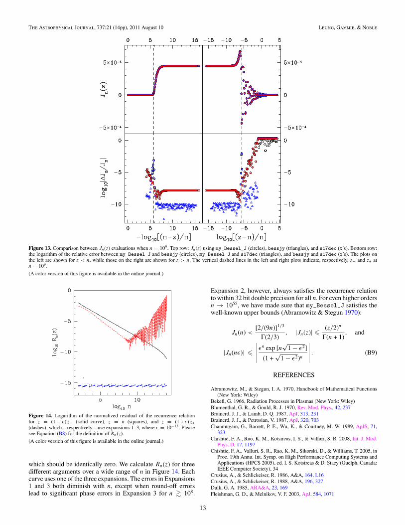
In Figure 13, we compare Jn(z) at n = 109 to see how thethree best methods compare with each other at large ordersover a wide range in argument. The fact that my_Bessel_Jagrees better with s17dec than does bessjy gives credenceto our method. The imperfectness of the transitions from oneexpansion to another exhibits itself by narrow peaks in therelative error between my_Bessel_J and the other methods.These peaks lie immediately about the transition points, whichare indicated by the dashed vertical lines. As z increases past n,round-off errors lead to significant phase errors. my_Bessel_Jand s17dec both follow the asymptotically sinusoidal trend atlarge z, but bessjy eventually returns with 0 and indicates thatit has reached its reliable limit.

To measure the accuracy at even larger orders, we employ therecurrence relation

2n

zJn(z) = Jn−1(z) − Jn+1(z) (B7)

and calculate the normalized deviation from it:

Rn(z) =∣∣∣∣ 1

Jn(z)

(2n

zJn(z) − Jn−1(z) − Jn+1(z)

)∣∣∣∣ , (B8)

7 The runtime for s17dec is constant up to n ∼ 104, after which it is a largerconstant.

12

The Astrophysical Journal, 737:21 (14pp), 2011 August 10 Leung, Gammie, & Noble

Figure 13. Comparison between Jn(z) evaluations when n = 109. Top row: Jn(z) using my_Bessel_J (circles), bessjy (triangles), and s17dec (x’s). Bottom row:the logarithm of the relative error between my_Bessel_J and bessjy (circles), my_Bessel_J and s17dec (triangles), and bessjy and s17dec (x’s). The plots onthe left are shown for z < n, while those on the right are shown for z > n. The vertical dashed lines in the left and right plots indicate, respectively, z− and z+ atn = 109.

(A color version of this figure is available in the online journal.)

Figure 14. Logarithm of the normalized residual of the recurrence relationfor z = (1 − ε) z− (solid curve), z = n (squares), and z = (1 + ε) z+(dashes), which—respectively—use expansions 1–3, where ε = 10−13. Pleasesee Equation (B8) for the definition of Rn(z).

(A color version of this figure is available in the online journal.)

which should be identically zero. We calculate Rn(z) for threedifferent arguments over a wide range of n in Figure 14. Eachcurve uses one of the three expansions. The errors in Expansions1 and 3 both diminish with n, except when round-off errorslead to significant phase errors in Expansion 3 for n � 108.

Expansion 2, however, always satisfies the recurrence relationto within 32 bit double precision for all n. For even higher ordersn → 1055, we have made sure that my_Bessel_J satisfies thewell-known upper bounds (Abramowitz & Stegun 1970):

Jn(n) <[2/(9n)]1/3

Γ(2/3), |Jn(z)| � (z/2)n

Γ(n + 1), and

|Jn(nε)| �∣∣∣∣∣ε

n exp [n√

1 − ε2]

(1 +√

1 − ε2)n

∣∣∣∣∣ . (B9)

REFERENCES

Abramowitz, M., & Stegun, I. A. 1970, Handbook of Mathematical Functions(New York: Wiley)

Bekefi, G. 1966, Radiation Processes in Plasmas (New York: Wiley)Blumenthal, G. R., & Gould, R. J. 1970, Rev. Mod. Phys., 42, 237Brainerd, J. J., & Lamb, D. Q. 1987, ApJ, 313, 231Brainerd, J. J., & Petrosian, V. 1987, ApJ, 320, 703Chanmugam, G., Barrett, P. E., Wu, K., & Courtney, M. W. 1989, ApJS, 71,

323Chishtie, F. A., Rao, K. M., Kotsireas, I. S., & Valluri, S. R. 2008, Int. J. Mod.

Phys. D, 17, 1197Chishtie, F. A., Valluri, S. R., Rao, K. M., Sikorski, D., & Williams, T. 2005, in

Proc. 19th Annu. Int. Symp. on High Performance Computing Systems andApplications (HPCS 2005), ed. I. S. Kotsireas & D. Stacy (Guelph, Canada:IEEE Computer Society), 34

Crusius, A., & Schlickeiser, R. 1986, A&A, 164, L16Crusius, A., & Schlickeiser, R. 1988, A&A, 196, 327Dulk, G. A. 1985, ARA&A, 23, 169Fleishman, G. D., & Melnikov, V. F. 2003, ApJ, 584, 1071

13

The Astrophysical Journal, 737:21 (14pp), 2011 August 10 Leung, Gammie, & Noble

Galassi, M., Davies, J., Theiler, J., Gough, B., Jungman, G., Booth, M., & Rossi,F. 2006, GNU Scientific Library Reference Manual (2nd ed.; Boston: FreeSoftware Foundation), http://www.gnu.org/software/gsl/

Ginzburg, V. L. 1970, The Propagation of Electromagnetic Waves in Plasmas(2nd ed.; Oxford: Pergamon)

Ginzburg, V. L., & Syrovatskii, S. I. 1968, Ap&SS, 1, 442Kawabata, K. 1964, PASJ, 16, 30Mahadevan, R., Narayan, R., & Yi, I. 1996, ApJ, 465, 327Marcowith, A., & Malzac, J. 2003, A&A, 409, 9Meggitt, S. M. A., & Wickramasinghe, D. T. 1982, MNRAS, 198, 71Melia, F. 1994, ApJ, 426, 577Melrose, D. B. 1989, Instabilities in Space and Laboratory Plasmas (Cambridge:

Cambridge Univ. Press)Melrose, D. B., & McPhedran, R. C. 1991, Electromagnetic Processes in

Dispersive Media (Cambridge: Cambridge Univ. Press)Noble, S. C., Leung, P. K., Gammie, C. F., & Book, L. G. 2007, Class. Quantum

Grav., 24, 259Pacholczyk, A. G. 1970, Radio Astrophysics: Nonthermal Processes in Galactic

and Extragalactic Sources (San Francisco, CA: Freeman)

Petrosian, V. 1981, ApJ, 251, 727Petrosian, V., & McTiernan, J. M. 1983, Phys. Fluids, 26, 3028Press, W. H., Teukolsky, S. A., Vetterling, W. T., & Flannery, B. P. 1992,

Numerical Recipes in C: The Art of Scientific Computing (Cambridge:Cambridge Univ. Press)

Robinson, P. A., & Melrose, D. B. 1984, Aust. J. Phys., 37, 675Rybicki, G. B., & Lightman, A. P. 1979, Radiative Processes in Astrophysics

(New York: Wiley)Scheuer, P. A. G. 1968, ApJ, 151, L139Schlickeiser, R., & Lerche, I. 2007, A&A, 476, 1Schott, G. A. 1912, Electromagnetic Radiation (Cambridge: Cambridge Univ.

Press)Stix, T. H. 1992, Waves in Plasmas (New York: AIP)Takahara, F., & Tsuruta, S. 1982, Prog. Theor. Phys., 67, 485Vath, H. M., & Chanmugam, G. 1995, ApJS, 98, 295Wardzinski, G., & Zdziarski, A. 2000, MNRAS, 314, 183Westfold, K. C. 1959, ApJ, 130, 241Wolfe, B., & Melia, F. 2006, ApJ, 637, 313

14