numerical and experimental study of a novel concept for ... identi cation and control, vol. 37, no....

Modeling, Identification and Control, Vol. 37, No. 4, 2016, pp. 195–211, ISSN 1890–1328

Numerical and Experimental Study of a NovelConcept for Hydraulically Controlled Negative

Loads

Jesper Kirk Sørensen 1 Michael Rygaard Hansen 1 Morten Kjeld Ebbesen 1

Department of Engineering Sciences, Faculty of Engineering and Science, University of Agder Jon Lilletunsvei 9,4879 Grimstad, Norway. E-mail: [email protected], [email protected], [email protected]

Abstract

This paper presents a numerical and experimental investigation of a novel concept that eliminates oscil-lations in hydraulic systems containing a counterbalance valve in series with a pressure compensated flowsupply. The concept utilizes a secondary circuit where a low-pass filtered value of the load pressure is gen-erated and fed back to the compensator of the flow supply valve. The novel concept has been implementedon a single boom actuated by a cylinder. A nonlinear model of the system has been developed and anexperimental verification shows good correspondence between the model and the real system. The modelis used for a parameter study on the novel concept. From the study it is found that the system is stablefor large directional valve openings and that for small openings a reduction of the oscillatory behaviour ofthe system can be obtained by either lowering the eigenfrequency of the mechanical-hydraulic system orby lowering the pilot area ratio of the counterbalance valve.

Keywords: counterbalance valve, pressure compensated valve, instabilities in hydraulic systems, nonlinearmodel, load-holding application

1 Introduction

For safety reasons, hydraulic load carrying applicationsare required by law to contain a load holding protectiondevice. The most widely used device is the counterbal-ance valve (CBV). It is multi-functional and providesleak tight load holding, load holding at hose/pump fail-ure as well as shock absorption, overload protection,and cavitation prevention at load lowering. However,it is well known that a series connection of a pressurecompensator (CV), a directional control valve (DCV),and a CBV tends to introduce instability in a system,see Miyakawa (1978), Persson et al. (1989), Handrooset al. (1993), Zahe (1995) and Hansen and Andersen(2010). This is mainly a problem when the controlledactuator is subjected to a negative load, i.e., a loadthat tends to drive the actuator as a pump, because

this will require the counterbalance valve to throttlethe return flow, see Figure 1. The system in Figure 1will be referred to as the base circuit.

It is a major challenge within hydraulic system de-sign to find solutions that offer stable handling ofnegative loads together with pressure compensatedmetering-in flow. Typically, practical solutions willcompromise either the load independency, the responsetime or the level of oscillations (Hansen and Andersen(2001) and Nordhammer et al. (2012)). The conse-quences of the oscillatory nature of such systems arereduced safety, reduced productivity as well as addedfatigue load on both the mechanical and hydraulic sys-tem. The severity of oscillations is affected by a widevariety of parameters some of which are hard to pre-dict or change: the external load on the actuator, theproperties of the mechanical structure, the friction in

doi:10.4173/mic.2016.4.1 c© 2016 Norwegian Society of Automatic Control

http://dx.doi.org/10.4173/mic.2016.4.1

Modeling, Identification and Control

AB

CBV

High pressureReturn pressure

CV

DCV

Figur 1

Figure 1: The base circuit consisting of a pressure com-pensator (CV), a directional control valve(DCV), a counterbalance valve (CBV), anda cylinder subjected to a compressing load.

the cylinder, the damping and hysteresis of the CBV,the operator input as well as volumes and restrictionsin the hydraulic lines. The efforts to minimize the os-cillatory nature of the base circuit can be divided intothree groups: Parameters variations (pilot area ratio ofCBV, pilot line orifices, etc.) on the circuit using thesame main components. The parameters with most in-fluence on the stability are the damping of the systemand the pilot ratio of the CBV (Hansen and Ander-sen, 2001). However lowering the pilot ratio of theCBV to minimize the oscillations will increase pres-sure levels and hence increase power consumption – es-pecially with small external loads. Another approachis to add damping when designing the pilot line lead-ing in to the CBV. However, no unique solution hasemerged that is useful across applications and workingconditions. A different approach is to actively compen-sate for the oscillations by applying closed-loop controlstrategies that involve the input signal to the DCV andsome kind of pressure feedback (Hansen and Ander-sen (2010), Cristofori et al. (2012) and Ritelli andVacca (2014)). The most important limitation in thesestrategies is the bandwidth limitation in typical DCVs.Alternatively, the pressure compensator (CV) can beremoved and the DCV replaced by a servo valve whichis a proven and reliable method for motion control. Theweaknesses here are in the investment costs and the dif-ficulties in handling disturbances in the supply pressure

caused by neighbouring circuits. The authors have in-vestigated the use of a DCV with compensated supplypressure, see Sørensen et al. (2014) and Sørensen et al.(2015). This is a commercially available alternativethat is characterized by low cost but also load depen-dent flow. Another example is described in Nordham-mer et al. (2012), where the main throttling ability ismoved from the CBV to the return orifice of the DCV,thereby eliminating the oscillations. However, this isnot a viable solution if the minimum load is 60% or lessof the maximum load, which strongly minimizes theapplicability. All of the approaches have certain draw-backs as compared to the base circuit. The authorshave previously presented a novel concept for address-ing this stability issue (Sørensen et al., 2016). It hasthe same steady state flow characteristics as the basecircuit only without the corresponding oscillatory na-ture. The concept was implemented on an experimen-tal setup and its ability to suppress oscillations wasexperimentally verified. This paper is devoted to thenonlinear modelling of the new concept with a view toinvestigate and predict the performance of the conceptwith special emphasis on stability.

2 Novel concept

In Figure 2 a hydraulic diagram of the proposed con-cept is shown, patent pending (Hansen and Sørensen,2015). It is shown in a situation where the actuator issubjected to a negative load, i.e., a lowering motion ofsome gravitational payload.

When compared to the base circuit in Figure 1, itcan be seen that the pilot pressure connection of theCV is supplied by the secondary circuit rather thanby the B-port pressure. The underlying idea is tosuppress oscillations in the system by generating thesteady state value of the B-port pressure in the sec-ondary circuit, filtering out any oscillations. The con-cept also encompasses solutions where the secondarycircuit is connected to the CBV or both the CV andthe CBV. The version used in this paper where only theCV is connected to the secondary circuit, is howeverthe preferred one from a reliability point of view. Thisis because the CBV and the related safety functions areactivated independent of any electrical system. Sincethe concept is passive as seen from the operator’s pointof view it can be combined with any closed loop con-trol strategies on the DCV. In this paper, the conceptpresented is with a linear actuator, but the methodwill also work for rotational actuators in circuits withcounterbalance valves.

The concept employs an orifice and a proportionalpressure relief valve (PV) in series. The intermedi-ate pressure, pC , is connected to the CV and will be

196

Sørensen et.al., “Numerical and Experimental Study of a Novel Concept for Hydraulically ...”

Figur 4

AB

CBV


CV

DCV

Secondary circuit

PV

Figure 2: Hydraulic diagram of novel concept wherethe CV is connected to the secondary circuit.

referred to as the compensator pressure. The overalltarget is that pC shall be the steady state value ofpB thereby suppressing oscillations of the compensatorand, subsequently, in the entire system. For that pur-pose, a control strategy is suggested that requires themeasurement of pB , a low-pass filtering yielding a ref-erence value for the compensator pressure, prefC and ameasurement of pressure, pC . This allows for a closedloop control where the pressure setting of the propor-tional pressure relief valve is adjusted by means of acontrol signal, uPV , in order to continuously meet thereference value of the compensator pressure. A blockdiagram of the used control strategy is shown in Fig-ure 3.

PV CVFilter

Pressure source

Figur 5

Figure 3: The proposed control strategy.

Figure 4 demonstrates the effect of the concept. Itcompares the pressures on both sides of the cylinder forthe base circuit and the concept when providing a rampinput downwards to a simple load-carrying boom, seefurther details in section 3. The base circuit is unstable

and the ability of the concept to suppress oscillationsin a real system is clear.

t [s]

0 2 4 6 8

Pre

ssur

e [b

ar]

-20

0

20

40

60

80

100

120

140

pA

pB

pA (Novel concept)

pB (Novel concept)

Figure 4: Comparison of pressures between the basecircuit and the system with the novel con-cept implemented for a DCV ramp input.

3 Considered system

In order to examine the concept in more detail investi-gations have been conducted on a setup in the mecha-tronics laboratory at the University of Agder, see Fig-ure 5. The setup consists of a hydraulically actuatedboom and a control system.

Cylinder

Bearing

Load

Figur 6

Figure 5: Hydraulic boom experimental setup.

The hydraulics can easily be altered from the novelconcept in Figure 2 to the base circuit in Figure 1.

197


The concept has been implemented using commerciallyavailable components. The DCV and CV are embed-ded in a pressure compensated 4/3-way directional con-trol valve group from Danfoss (Model: PVG32). Ithas an electrohydraulic actuation with linear flow vs.input signal characteristics with a maximum value ofQmaxDCV = 25L/min. The 4-port CBV is from SunHydraulics (Model: CWCA) with a 3:1 pilot area ra-tio and a rated flow of QrCBV = 60L/min. The PVis from Bosch Rexroth (Model: DBETE) and has acrack pressure that varies linearly with the voltage in-put. At maximum signal, umaxPV = 1, the valve cracksopen at pC@0L/min = 185bar and has a rated pres-sure prPV = [email protected]/min = 200bar. In Table 1 arelisted some other design parameters of the experimen-tal setup.

Table 1: Design parameters of the experimental setup.

Parameter Value

Distance from bearing tomass centre of boom + load.

L = 3570mm

Mass of boom + load m = 410kgCylinder stroke Hc = 500mmCylinder piston diameter Dp = 65mmCylinder rod diameter Dr = 35mm

Cylinder area ratio µC =D2

p

D2p−D2

r= 1.41

Supply pressure pS = 180bar

A real-time I/O system is used to control the hy-draulic valves on the boom with a loop time of 10ms.The control system can record sensor information fromall the position and pressure sensors mounted on thetest setup. The primary circuit is activated by supply-ing the directional control valve with an input signal.The purpose of the controller on the secondary circuitis to keep the compensator pressure, pC , in accordancewith the reference pressure prefC , in Figure 3. The fil-ter box uses the actual pB value as input and returnsprefC . The choice of filter frequency should of coursereflect both the dominant lowest eigenfrequency of themechanical-hydraulic system as well as the demand fora certain response time of the system. The role of thelow-pass filter is to remove oscillations, however if it ischosen overly conservative then the system reacts tooslowly. Therefore, some logic has been added so thatthe compensator reference pressure, prefC , never goesbelow a certain minimum value, pmin:

prefC =

{pmin , pB < pmin

pB,LPF , pB ≥ pmin(1)

where pB,LPF is the low-pass filtered value of pB :

pB,LPF =1

τ· (pB − pB,LPF ) (2)

The PI-controller has the classic form:

uPV = KP ·(prefC − pC) +

∫KI ·(prefC − pC)·dt (3)

where saturation and corresponding anti-windupmeasures (integrated effort not accumulated at satura-tion) are implemented so that 0 ≤ uPV ≤ 1. Basically,only four parameters need to be set: pmin, τ , KP andKI .

4 Nonlinear model

A nonlinear model of the system, both with and with-out the concept implemented, is developed using thecommercial simulation software SimulationX. This sec-tion describes the theory behind the different parts ofthis model.

4.1 Mechanical system

The mechanical system used in the investigation of theconcept for stabilizing the hydraulic circuit comprises aboom, a payload, a base, and a double acting hydraulicactuator – see Figure 6.

Boom Payload

Double acting cylinder

Base

Bearing Strain gauge

Figure 6: Mechanical system.

In the time domain simulation of the system theboom is modelled to be flexible using the finite segmentmethod as described by Huston and Wang (1994). Themethod is now well tested for modelling the dynamicbehaviour of flexible beam systems in a relatively sim-ple way. In the finite segment method a beam is re-placed with a number of smaller beam segments con-nected to each other with extension and/or torsional

198


springs. With this method it is possible to model bothbending, extension, and torsion of a beam. The sys-tem at hand is considered to be a planar mechanismand only bending is taken into account. The flexibil-ity in the longitudinal direction of the beam is omit-ted as its influence on the dynamic behaviour of thesystem can be neglected. Therefore the segments inthe present model are connected by revolute joints andtorsional springs. Due to the segmented nature of themodel it does not describe the deformed shape of thebeam smoothly but this is not required for the prob-lem at hand where the key point of interest is systemoscillations. The segmented structure is illustrated inFigure 7.

ki keq,ijki ki

i i j

Ls,i

k

keq,jk

ceq,ij ceq,jk

kk

Revolute joint

Rotational damper

Figure 7: Illustration of torsional springs and dampersbetween segments in the finite segmentmethod.

The torsional spring between two segments has thestiffness of two springs mounted in series. The stiffnesski of the spring related to segment number i can bewritten as:

ki =2 · E · IzLs,i

(4)

where E is the bulk modulus of the beam material,Iz is the 2nd moment of inertia for the cross sectionof the prismatic beam, and Ls,i is the length of thesegment. The equivalent spring stiffness keq,ij betweentwo segments can then be written as two springs inseries:

keq,ij =ki · kjki + kj

(5)

The number of segments in the model is a compro-mise between accuracy and computational time. Toobtain a sufficiently good approximation of the eigen-frequency of the boom the model contains four seg-ments between the bearing and cylinder and five seg-ments between the cylinder and the payload. The baseis considered to be rigid even though observations dur-ing the experimental work have revealed that the basealso contributes to the flexibility in the system. Toaccommodate the flexibility of the base a tuning fac-tor has been applied to the stiffnesses of the segmentsto tune the dynamic behaviour to experimental data.

The payload is considered to be a rigid point mass. Asillustrated in Figure 7 a rotational damper is also in-cluded in the connection between two segments. Thevalue of the damping coefficient, ceq, is found throughtuning to the experimental data.

4.2 Hydraulic system

The description of the hydraulic system is only devel-oped for downwards motion of the boom.

4.2.1 Directional control valve

The directional control valve unit consists of a direc-tional control valve in series with a pressure compen-sator valve. The valve has been modelled as two vari-able orifices as shown in Figure 8. The opening of theseare controlled by a set of function blocks, includingvalve dynamics.

Dead band compensation

CV steady stateequation

CVDynamics

Figur – DCV structure

DCV Dynamics

,

, ,

Figure 8: Structure of DCV model.

The blue lines are signal lines and the black lines arehydraulic lines. Assuming constant density and usingthe orifice flow equation then the flow across the DCVcan be computed as:

QDCV,in = kCS−B · uDCV ·√pCS − pB (6)

QDCV,out = kA−T · uDCV ·√pA − pT (7)

where QDCV,in and QDCV,out are the compensatedmetering-in flow and metering-out flow, pT is the tankpressure, uDCV is the dimensionless opening of thevalve. The parameters kCS−B and kA−T are valveconstants. The compensated supply pressure, pCS , iscalculated by the compensator equation, which is im-plemented like:

pCS1 =

{pS , pi ≥ pS − pDCV,clpi + pDCV,cl , pi < pS − pDCV,cl

(8)

where pi is the input pressure to the CV, pS is thesupply pressure and pDCV,cl is the nominal pressuredrop across the main spool (setting of CV spring). Thedynamics of the CV is added to account for the valve

199


not being a perfect flow source. It is described by afirst order transfer function:

pCSpCS1

(s) =1

τCV · s+ 1(9)

A difference between the model of the base circuitand the concept is the input pressure, pi, to the CV:

pi =

{pB , for Base Circuit

pC , for Novel Concept(10)

Experiments showed a slightly higher flow output ofthe DCV utilising the concept than of the base circuit.This indicates that equation (10) in reality looks like:

pi =

{pB −∆pBCLS (uDCV )

pC −∆pNCLS (uDCV )(11)

where ∆pLS is the pressure drop internally in theDCV’s load sensing system before the CV which is afunction of uDCV . The difference between the two sys-tems occurs because pressure pC is obtained by con-necting the secondary circuit to an external port onthe DCV, while pressure pB is handled internally in theDCV. The experiments indicate that ∆pBCLS > ∆pNCLS .The pressure drop ∆pLS , is combined with kCS−Bin an equivalent valve characteristic LCS−B , changingequation (6) to:

QBCDCV,in = LBCCS−B(uDCV ) ·√pCS − pB (12)

QNCDCV,in = LNCCS−B(uDCV ) ·√pCS − pB (13)

In Figure 9 is shown LCS−B for both systems as afunction of uDCV .

The spool is open-centre, hence, it has no dead bandon the outlet. For the inlet a dead band compensationis implemented as follows, where σDB is the dimension-less dead band:

uDCV,DB=

{0 , urefDCV =0

σDB+(1−σDB)·urefDCV , urefDCV >0(14)

The dynamics of the DCV is implemented using asecond order transfer function:

uDCVuDCV,DB

(s) =1

s2

ω2DCV

+ 2 · ζDCV · sωDCV

+ 1(15)

where ωDCV is the natural eigenfrequency of thevalve and ζDCV is the damping ratio. Values for theparameters used in the modelling work can be foundin Table 2.

uDCV

[-]

0 0.1 0.2 0.3 0.4L

CS

-B [l

/min·ba

r-1/2

]0

0.5

1

1.5

2

2.5

3

3.5

Base circuit

Novel concept

Figure 9: Equivalent valve characteristic, LCS−B , asfunction of uDCV .

Table 2: DCV model parameters.

Parameter Value

kA−T 2.3 Lmin√bar

pDCV,cl 7bara

τCV 0.0064sσDB 0.14ωDCV 30 rads (4.8Hz)ζDCV 0.8a

a Bak and Hansen (2013)

200


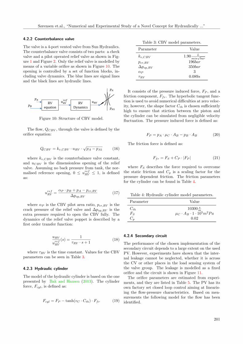
4.2.2 Counterbalance valve

The valve is a 4-port vented valve from Sun Hydraulics.The counterbalance valve consists of two parts: a checkvalve and a pilot operated relief valve as shown in Fig-ure 1 and Figure 2. Only the relief valve is modelled bymeans of a variable orifice as shown in Figure 10. Theopening is controlled by a set of function blocks, in-cluding valve dynamics. The blue lines are signal linesand the black lines are hydraulic lines.

controller

RV equation

RV Dynamics

Figur – CBV structure

Figure 10: Structure of CBV model.

The flow, QCBV , through the valve is defined by theorifice equation:

QCBV = kv,CBV · uRV ·√pA − pA1 (16)

where kv,CBV is the counterbalance valve constant,and uCBV is the dimensionless opening of the reliefvalve. Assuming no back pressure from tank, the nor-malised reference opening, 0 ≤ urefRV ≤ 1, is definedas:

urefRV =αP · pB + pA − pcr,RV

∆pop,RV(17)

where αP is the CBV pilot area ratio, pcr,RV is thecrack pressure of the relief valve and ∆pop,RV is theextra pressure required to open the CBV fully. Thedynamics of the relief valve poppet is described by afirst order transfer function:

uRV

urefRV(s) =

1

τRV · s+ 1(18)

where τRV is the time constant. Values for the CBVparameters can be seen in Table 3.

4.2.3 Hydraulic cylinder

The model of the hydraulic cylinder is based on the onepresented by Bak and Hansen (2013). The cylinderforce, Fcyl, is defined as:

Fcyl = FP − tanh(vC · Cth) · Ffr (19)

Table 3: CBV model parameters.

Parameter Value

kv,CBV 1.90 Lmin√bar

pcr,RV 196bar∆pop,RV 350barαP 3τRV 0.089s

It consists of the pressure induced force, FP , and afriction component, Ffr. The hyperbolic tangent func-tion is used to avoid numerical difficulties at zero veloc-ity, however, the shape factor Cth is chosen sufficientlyhigh to ensure that stiction between the piston andthe cylinder can be simulated from negligible velocityfluctuation. The pressure induced force is defined as:

FP = pA · µC ·AB − pB ·AB (20)

The friction force is defined as:

Ffr = FS + CP · |FP | (21)

where FS describes the force required to overcomethe static friction and Cp is a scaling factor for thepressure dependent friction. The friction parametersfor the cylinder can be found in Table 4.

Table 4: Hydraulic cylinder model parameters.

Parameter Value

Cth 10300 sm

FS µC ·AB · 1 · 105m2PaCp 0.02

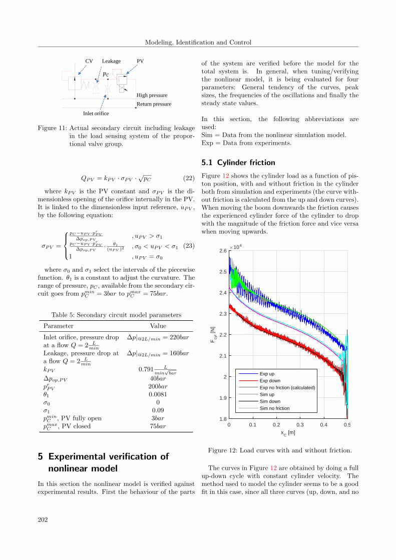
4.2.4 Secondary circuit

The performance of the chosen implementation of thesecondary circuit depends to a large extent on the usedPV. However, experiments have shown that the inter-nal leakage cannot be neglected, whether it is acrossthe CV or other places in the load sensing system ofthe valve group. The leakage is modelled as a fixedorifice and the circuit is shown in Figure 11.

The orifice parameters are estimated from experi-ments, and they are listed in Table 5. The PV has itsown factory set closed loop control aiming at linearis-ing the flow-pressure characteristics. Based on mea-surements the following model for the flow has beenidentified.

201


Return pressureHigh pressure

PVCV Leakage

Figur 7

Inlet orifice

Figure 11: Actual secondary circuit including leakagein the load sensing system of the propor-tional valve group.

QPV = kPV · σPV ·√pC (22)

where kPV is the PV constant and σPV is the di-mensionless opening of the orifice internally in the PV.It is linked to the dimensionless input reference, uPV ,by the following equation:

σPV =

pC−uPV ·prPV

∆pop,PV, uPV > σ1

pC−uPV ·prPV

∆pop,PV· θ1

(uPV )2 , σ0 < uPV < σ1

1 , uPV = σ0

(23)

where σ0 and σ1 select the intervals of the piecewisefunction. θ1 is a constant to adjust the curvature. Therange of pressure, pC , available from the secondary cir-cuit goes from pminC = 3bar to pmaxC = 75bar.

Table 5: Secondary circuit model parameters

Parameter Value

Inlet orifice, pressure dropat a flow Q = 2 L

min

∆p|@2L/min = 220bar

Leakage, pressure drop ata flow Q = 2 L

min

∆p|@2L/min = 160bar

kPV 0.791 Lmin√bar

∆pop,PV 40barprPV 200barθ1 0.0081σ0 0σ1 0.09pminC , PV fully open 3barpmaxC , PV closed 75bar

5 Experimental verification ofnonlinear model

In this section the nonlinear model is verified againstexperimental results. First the behaviour of the parts

of the system are verified before the model for thetotal system is. In general, when tuning/verifyingthe nonlinear model, it is being evaluated for fourparameters: General tendency of the curves, peaksizes, the frequencies of the oscillations and finally thesteady state values.

In this section, the following abbreviations areused:Sim = Data from the nonlinear simulation model.Exp = Data from experiments.

5.1 Cylinder friction

Figure 12 shows the cylinder load as a function of pis-ton position, with and without friction in the cylinderboth from simulation and experiments (the curve with-out friction is calculated from the up and down curves).When moving the boom downwards the friction causesthe experienced cylinder force of the cylinder to dropwith the magnitude of the friction force and vice versawhen moving upwards.

xC [m]

0 0.1 0.2 0.3 0.4 0.5

Fcy

l [N]

×104

1.8

1.9

2

2.1

2.2

2.3

2.4

2.5

2.6

Exp up

Exp down

Exp no friction (calculated)

Sim up

Sim down

Sim no friction

Figure 12: Load curves with and without friction.

The curves in Figure 12 are obtained by doing a fullup-down cycle with constant cylinder velocity. Themethod used to model the cylinder seems to be a goodfit in this case, since all three curves (up, down, and no

202


friction) show a similar pattern as the measured ones.This also shows that the mechanical loads in the modelare a good approximation of the real system.

5.2 Eigenfrequency

The pure mechanical eigenfrequency, fm, and dampingare found in the top and bottom position of the boom.In both of these experiments the piston is preloaded sothat it is mechanically fixed to the relevant cylinder endplate. Next, the boom is excited manually and the mo-tion is recorded. In Figure 13 the oscillations from theexperiments are compared to the ones achieved fromthe simulation. From the experimental setup, strain ismeasured in the boom, see Figure 6, and from the sim-ulation, the deflection of the nearby spring is used. Thetwo data sets have been normalised to have the sameamplitude at time t = 0s, see Figure 13. The compar-ison of strain and deflection respectively is consideredto be acceptable.

t [s]0 1 2 3 4 5 6

Nor

mal

ised

val

ue [-

]

-1

-0.5

0

0.5

1

Exp (strain)

Sim (spring deflection)

Figure 13: Normalised values of oscillations in top po-sition (xC = 0m).

The curves show a good correspondence betweensimulation and experiments. The model has a slightlyhigher eigenfrequency. Due to the fact that the base isnot included directly as a flexible part in the modellingof the mechanical structure but only as a tuning factor,the mechanical eigenfrequency from the model does notmatch the experiments perfectly over the entire spanof operation. However, the difference is acceptable, seeTable 6. The curves in Figure 13 also show that themechanical damping is in accordance.

Table 6: Mechanical eigenfrequencies, fm.

Position fm (Sim) fm (Exp)

Top 3.2Hz 3.2HzBottom 3.1Hz 3.2Hz

The next step is to look at the combined mechanical-hydraulic eigenfrequency, fmh, when the piston is sus-

pended by two oil column springs in parallel. For thatpurpose investigations are carried out for two charac-teristic piston positions, xC = 0.10m and xC = 0.25m,respectively. Figure 14 (upper) shows the normalisedvalues of oscillations when the boom is placed with thepiston at xC = 0.10m and a similar external force asbefore is applied to verify the spring effect of the hy-draulic system. As it can be seen, the oscillations showa nice fit, including the damping. However, a variancein eigenfrequency is noticed. During the first second,the curves coincide, then the oscillations of the simula-tion are slowing down compared to the measured valuesbefore finally ending a bit faster than the experimentalones. To illustrate this, the frequency of each periodis shown as a function of time in Figure 14 (lower),where the mentioned difference is visible. This varyingeigenfrequency of the boom is a result of the friction.As time elapses and the oscillatory motion dampensout then the stiction period where the piston and thecylinder are locked together increases until it coversthe entire oscillation time. In that period, the eigen-frequency increases from the mechanical-hydraulic tothe pure mechanical that can also be found in Table 6.Because of the small deviations from the experimentsand the good correlation in how the stiction influencesthe overall motion, the model is considered useful fora parameter study.

0 1 2 3 4 5 6

Nor

mal

ised

val

ue [-

]

-1

-0.5

0

0.5

1

Exp (strain)


t [s]0 1 2 3 4 5 6

f mh [H

z]

2.6

2.8

3

3.2

Figure 14: (Upper) Normalised values of oscillations atxC = 0.10m. (Lower) Mechanical-hydrauliceigenfrequency fmh, showing the frequencybetween each downwards zero crossing ofthe upper figure.

203


For xC = 0.25m the same tendency is observed, seeFigure 15. It is also noticed that the damping rate islower in this position, due to the change in cylindervolumes.

t [s]0 1 2 3 4 5 6

f mh [H

z]

2.6

2.8

3

3.2

Exp (strain)


Figure 15: Mechanical-hydraulic eigenfrequency atxC = 0.25m. The plot shows the frequencybetween each downwards zero crossingof a curve of the normalised values ofoscillations at xC = 0.25m.

The lower limit for the mechanical-hydraulic eigen-frequency can be found by removing the cylinder fric-tion in the simulation. In Figure 16 this fNFmh is shownas a function of the piston position.

xC [m]

0 0.1 0.2 0.3 0.4 0.5

f mh

NF

[Hz]

2.4

2.6

2.8

Sim, No cylinder friction

Figure 16: Mechanical-hydraulic eigenfrequency with-out cylinder friction, fNFmh as a function ofpiston position xC .

5.3 Secondary circuit

In order to be able to verify the performance of thenovel concept the secondary circuit is analysed first.To check the model of the PV in equation (23), it iscompared to experimental values when pC is plotted asa function of uPV , see Figure 17.

The experiment shows that an input uPV to themodel gives the expected pressure pC . The perfor-mance is evaluated by applying a reference step in-put, prefC , of 40bar to the secondary circuit. With

uPV

[-]

0 0.05 0.1 0.15 0.2 0.25 0.3 0.35

pC [b

ar]

0

20

40

60

80

Exp

Sim

Figure 17: Verification of the PV: Pressure pC as afunction of uPV .

pmin = 5bar, the gains were adjusted to: KP = 0.01 Vbar

and KI = 0.04 Vbar·s . The results are shown in Fig-

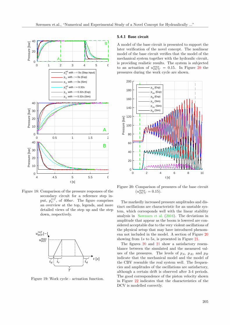
ure 18.The experiment consists of two parts: one where the

unfiltered performance of the secondary circuit is eval-uated and one where the low-pass filter is applied. Theblue curve shows the reference step input. The abilityof the closed-loop control system to follow this refer-ence is shown in red and black, for the experiment andsimulation. These curves are obtained without any fil-tration, i.e., τ = 0s. The performance when applyingthe low-pass filter in the system is the other part. Thefiltered reference prefC with a cut-off frequency set toτ = 0.32s, is shown in cyan. The remaining curves,the green and magenta show the ability of pC to followthis prefC . In both cases, the model shows good confor-mity with the experiments both when stepping up anddown.

5.4 Total system

To achieve a uniform evaluation of the total system astandard actuation of the DCV is used in the following,see Figure 19. Only situations where the cylinder isretracting are investigated.

The actuation is defined by the cycle time, T , a delaytime to ensure static conditions, td, the ramp time, tr,and the wanted steady state DCV input umaxDCV . Thetime parameters are equal for all tests, see Table 7.

In the reminder of the verification section, thedashed green lines in the figures indicate when urefDCV 6=0.

Table 7: Common parameters for all actuation.

Cycle time, T Ramp time, tr Time delay, td

8s 1s 1s

204


0 1 2 3 4 5 6

Pre

ssur

e [b

ar]

0

20

40

A

B

pCref with τ = 0s (Step input)

pC with τ = 0s (Exp)

pC with τ = 0s (Sim)

pCref with τ = 0.32s

pC with τ = 0.32s (Exp)

pC with τ = 0.32s (Sim)

0 0.5 1 1.5 2

Pre

ssur

e [b

ar]

0

10

20

30

40

A

t [s]

4 4.5 5 5.5 6

Pre

ssur

e [b

ar]

0

10

20

30

40B

Figure 18: Comparison of the pressure responses of thesecondary circuit for a reference step in-put, prefC , of 40bar. The figure comprisesan overview at the top, legends, and moredetailed views of the step up and the stepdown, respectively.

Figur 11

Figure 19: Work cycle - actuation function.

5.4.1 Base circuit

A model of the base circuit is presented to support thelater verification of the novel concept. The nonlinearmodel of the base circuit verifies that the model of themechanical system together with the hydraulic circuit,is providing realistic results. The system is subjectedto an actuation of umaxDCV = 0.15. In Figure 20 thepressures during the work cycle are shown.

t [s]

0 2 4 6 8 10

Pre

ssur

e [b

ar]

0

20

40

60

80

100

120

140

160

180

200

pA (Exp)

pA1 (Exp)

pB (Exp)

pA (Sim)

pA1 (Sim)

pB (Sim)

Figure 20: Comparison of pressures of the base circuit(umaxDCV = 0.15).

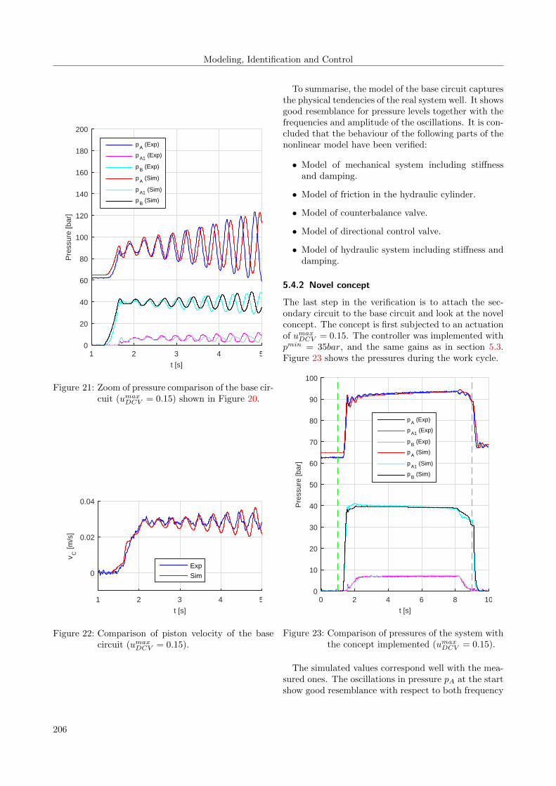
The markedly increased pressure amplitudes and dis-tinct oscillations are characteristic for an unstable sys-tem, which corresponds well with the linear stabilityanalysis in Sørensen et al. (2016). The deviations inamplitude that appear as the boom is lowered are con-sidered acceptable due to the very violent oscillations ofthe physical setup that may have introduced phenom-ena not included in the model. A section of Figure 20showing from 1s to 5s, is presented in Figure 21.

The figures 20 and 21 show a satisfactory resem-blance between the simulated and the measured val-ues of the pressures. The levels of pA, pA1 and pBindicate that the mechanical model and the model ofthe CBV resemble the real system well. The frequen-cies and amplitudes of the oscillations are satisfactory,although a certain drift is observed after 3-4 periods.The good correspondence of the piston velocity shownin Figure 22 indicates that the characteristics of theDCV is modelled correctly.

205


t [s]

1 2 3 4 5

Pre

ssur

e [b

ar]

0

20

40

60

80

100

120

140

160

180

200

pA (Exp)

pA1 (Exp)

pB (Exp)

pA (Sim)

pA1 (Sim)

pB (Sim)

Figure 21: Zoom of pressure comparison of the base cir-cuit (umaxDCV = 0.15) shown in Figure 20.

t [s]

1 2 3 4 5

v C [m

/s]

0

0.02

0.04

Exp

Sim

Figure 22: Comparison of piston velocity of the basecircuit (umaxDCV = 0.15).

To summarise, the model of the base circuit capturesthe physical tendencies of the real system well. It showsgood resemblance for pressure levels together with thefrequencies and amplitude of the oscillations. It is con-cluded that the behaviour of the following parts of thenonlinear model have been verified:

• Model of mechanical system including stiffnessand damping.

• Model of friction in the hydraulic cylinder.

• Model of counterbalance valve.

• Model of directional control valve.

• Model of hydraulic system including stiffness anddamping.

5.4.2 Novel concept

The last step in the verification is to attach the sec-ondary circuit to the base circuit and look at the novelconcept. The concept is first subjected to an actuationof umaxDCV = 0.15. The controller was implemented withpmin = 35bar, and the same gains as in section 5.3.Figure 23 shows the pressures during the work cycle.

t [s]

0 2 4 6 8 10

Pre

ssur

e [b

ar]

0

10

20

30

40

50

60

70

80

90

100

pA (Exp)

pA1 (Exp)

pB (Exp)

pA (Sim)

pA1 (Sim)

pB (Sim)

Figure 23: Comparison of pressures of the system withthe concept implemented (umaxDCV = 0.15).

The simulated values correspond well with the mea-sured ones. The oscillations in pressure pA at the startshow good resemblance with respect to both frequency

206


and amplitude. There are minor differences betweenmodel and simulation in both pressure pA and pB whenthe deceleration begins after 8s, but the general trend isfollowed and the pressures are deemed satisfying. Thepressures of the secondary circuit are shown in Fig-ure 24.

t [s]

0 2 4 6 8 10

Pre

ssur

e [b

ar]

20

30

40

50

60

pC (Exp)

pC (Sim)

pB (Exp)

Figure 24: Pressure response of the concept’s sec-ondary circuit during work cycle (umaxDCV =0.15).

The pressure peaks at the beginning and end of thecycle which only occur in the experiments, indicatethat modelling the leakage as a fixed orifice might be anoversimplification of the LS system. A detailed analy-sis of this would lie outside the scope of this paper andis also considered peripheral to the more generic inves-tigation of the concept. The measured pressure pB inthe diagram is added to illustrate how the secondarycircuit reacts to inputs from the primary circuit. Com-paring the piston position and velocity in Figure 25and Figure 26, a good resemblance is observed in bothfigures; for example is the small peak with negative ve-locity measured in the experiments at approximately9s replicated in the simulation.

t [s]

0 2 4 6 8 10

x C [m

]

0.1

0.2

0.3

Exp

Sim

Figure 25: Comparison of piston position of the systemwith the concept implemented (umaxDCV =0.15).

t [s]

0 2 4 6 8 10

v C [m

/s]

0

0.02

0.04

Exp

Sim

Figure 26: Comparison of piston velocity of the systemwith the concept implemented (umaxDCV =0.15).

To add further depth to the verification of the model,an actuation of umaxDCV = 0.05 is also analysed. Fig-ure 27 shows the pressures during this work cycle.

t [s]

0 2 4 6 8 10

Pre

ssur

e [b

ar]

0

10

20

30

40

50

60

70

80

90

100

pA (Exp)

pA1 (Exp)

pB (Exp)

pA (Sim)

pA1 (Sim)

pB (Sim)

Figure 27: Comparison of pressures of the system withthe concept implemented (umaxDCV = 0.05).

Also in this case the simulated values correspond wellwith the measured ones. However, the amplitudes aresmaller in the simulation for both pressure pA and pB ,and this is most pronounced at the rod side of thecylinder. Figure 28 highlights this part of the pressurecurve.

There is a certain discrepancy which was not seenfor the base circuit, hence, the source for this devi-ation probably lies in the modelling of the modified

207


t [s]

2 2.5 3 3.5 4 4.5 5

Pre

ssur

e [b

ar]

32

34

36

38

40

pB (Exp)

pB (Sim)

Figure 28: Zoom of part of pressure pB from the systemwith the concept implemented (umaxDCV =0.05) shown in Figure 27.

DCV. As seen in Figure 24 the modifications have ledto pressure fluctuations in the secondary circuit noteasily accounted for and it may be the same phenom-ena that give more oscillations in the rod side volume ofthe physical system. Finally, the flow capability of theDCV is checked by comparing the steady state velocityof the piston. Experiments using the work cycle func-tion for nine different values of umaxDCV were conducted.The result of the tailor-made flow characteristics intro-duced in equation (13) can be seen in Figure 29, clearlyindicating that the deviations are virtually eliminated.

uDCVref [-]

0 0.1 0.2 0.3 0.4

v C [m

/s]

0

0.01

0.02

0.03

0.04

0.05

0.06

EvC

[m/s

]

×10-4

-3

-2

-1

0

1

2

3

Figure 29: Simulated steady state piston velocities fordifferent valve openings for the system withthe concept implemented. The velocity er-ror EvC = vC(Exp)− vC(Sim).

A nonlinear simulation model has been developedfor the novel concept applied as actuation for a specificcylinder-boom mechanism. In general, the model cor-responds well both steady state and dynamically withmeasured data and it is further validated by simula-tions and experiments conducted using a base circuitas actuation for the same mechanism.

6 Parameter study

The nonlinear model is utilised to investigate whichparameters yield the largest influence on the stabilityof the novel concept. A linear stability analysis hasindicated that small openings of the directional con-trol valve result in stability issues (Sørensen et al.,2016). That linear analysis was, however, based on asimplified system and therefore a parameter study isconducted here with a view to investigate the oscilla-tory behaviour of the nonlinear system. Since stabilityis associated with linear systems the term is adaptedto the current study based on how the pressure am-plitudes develop after the ramp up is conducted, i.e.urefDCV = umaxDCV . Increasing amplitudes are clearly char-acteristics of a highly oscillatory system in this contextand are simply referred to as unstable. The way theconcept is working with the secondary circuit separatedfrom the primary circuit by a low-pass filter lowers theperformance requirements to the components in thesecondary circuit, hence its influence on the stabilityof the system is limited. The cylinder friction does notyield much effect on the stability either. Simulationsshow that the parameters most influential on the sys-tems stability are the stiffness of the mechanical struc-ture and the pilot area ratio of the CBV. In Figure 30the blue curve shows the minimum urefDCV yielding astable system as a function of fNFmh when the startingposition of the piston is xC = 0.10m. The system be-comes increasingly oscillatory when the stiffness andhence the eigenfrequency increases. Also notice thatfor fNFmh < 2.2Hz the simulation becomes stable for allvalve openings.

fmhNF [Hz]

1.5 2 2.5 3 3.5

uD

CV

ref

[-]

0

0.05

0.1

CV

CV + CBV

Figure 30: Stability of the nonlinear model of thenovel concept; both connected to CV andCV+CBV. The diagram shows the mini-mum urefDCV that yields a stable system asa function of fNFmh for αP = 3. The dashedmagenta line is the value of the real system.

Curves for a varying pilot area ratio of the CBV areshown in Figure 31. Stability is improved by lowering

208


the pilot area ratio. This of course happens at the ex-pense of a more pronounced pressure-load dependencyin the cylinder chambers. The blue curve also indicatesthat for pilot ratios αP < 1.9 stability can be ensuredin all cases.

αP [-]

1 2 3 4 5

uD

CV

ref

[-]

0

0.05

0.1

CV

CV + CBV

Figure 31: Stability of the nonlinear model of thenovel concept; both connected to CV andCV+CBV. The diagram shows the mini-mum urefDCV that yields a stable system asa function of αP for fNFmh = 2.5Hz. Thedashed magenta line is the value of the realsystem.

In both Figure 30 and Figure 31 the curves for CVindicate that for the system in the lab (fNFmh = 2.5Hz

and αP = 3) instability occurs for urefDCV below approx-imately 0.04, for this specific system. In some appli-cations, the possible risk of oscillations for small valveopenings might be unacceptable. As mentioned in thepresentation of the concept the solution also encom-passes a version where the secondary circuit besidesbeing connected to the CV also controls the opening ofthe CBV (CV+CBV). The hydraulic diagram of thiscircuit is shown in Figure 32.

The results of this change in the hydraulic circuit areshown in red in Figure 30 and Figure 31. If αP = 3, thissolution does not experience instability for any valueof fNFmh . When varying the pilot area ratio, a clearimprovement can be observed. The stability thresholdincreases and the system is now stable in the config-uration of the real setup (αP = 3). This proves thatthe concept is able to stabilise the experimental setupfor all openings of the directional control valve. Con-trolling the opening area of the CBV via a separatepressure source can be regarded problematic from areliability point of view in some applications, since theCBV provides different safety functions, among themload holding at hose/pump failure. Therefore, the so-lution indicated in Figure 32 should only be consideredif instability cannot be overcome by lowering the pilotarea ratio.

Secondary circuit

Figur 3

AB

CBV


CV

DCV

Figure 32: Hydraulic diagram of novel concept. Boththe CBV and the CV are connected to thesecondary circuit.

7 Conclusions

The authors have previously presented a novel conceptcapable of suppressing oscillations in hydraulic systemscontaining a CBV and a pressure compensated direc-tional control valve (DCV), see Sørensen et al. (2016).The concept utilizes a secondary circuit where a low-pass filtered value of the load pressure is generatedand fed back to the compensator of the flow supplyvalve. This paper has focused on a further investiga-tion of this concept and limitations hereof. A non-linear dynamic model has been developed and exper-imentally verified on a cylinder actuated single boommechanism. The commercial simulation tool Simula-tionX has been used as platform for the modeling. Themechanical system is modelled as a multi-body systemusing the finite segment flexibility method. The hy-draulic circuit including the main control componentshave been modelled using a combination of liquid vol-umes, variable orifices and 1st and 2nd order trans-fer functions to capture valve dynamics. The eigen-frequencies of both the mechanical and the combinedmechanical-hydraulic system and the secondary circuitwere investigated and validated separately - before be-ing combined to a model of the entire system. In or-der to strengthen the verification, a model of the samemechanical-hydraulic system actuated by means of astandard base circuit was also investigated both experi-mentally and numerically. This ensured that the devel-

209


oped models of the mechanical system and the counter-balance valve (CBV) could be verified for two differentsetups. The full nonlinear model of the mechanical-hydraulic system actuated by the concept was in gen-eral, in good accordance with measurements. Duringthe modelling of the mechanical-hydraulic system inthis paper the following areas showed themselves to beof high importance:

• Flexibility of the mechanical system.

• Friction in the hydraulic cylinder.

• Continuous opening of the CBV.

• Proper characteristics of the DCV.

Since the main feature of the concept is its ability tosuppress oscillations, the developed model was used fora parameter study with emphasis on instability. Themodel confirmed the results from the linear analysis inSørensen et al. (2016), that there is an elevated risk forinstability at small DCV openings. The model showsthat an improved system stability can be obtained byeither reducing the eigenfrequency of the mechanical-hydraulic system or lowering the pilot area ratio of theCBV. Finally, the model showed the improved stabilitycharacteristics of another version of the concept wherealso the CBV pilot port is connected to the low passfiltered load pressure. This version would normally beconsidered less desirable from a reliability point of viewbecause the basic safety features of the CBV are con-trolled electronically, however, the simulations indicatethat it could be an alternative for systems that cannotbe stabilised otherwise.

Acknowledgments

The work is funded by the Norwegian Ministry of Ed-ucation & Research and National Oilwell Varco.

References

Bak, M. K. and Hansen, M. R. Analysis of off-shore knuckle boom crane - part one: Mod-eling and parameter identification. Modeling,Identification and Control, 2013. 34(4):157–174.doi:10.4173/mic.2013.4.1.

Cristofori, D., Vacca, A., and Ariyur, K. Anovel pressure-feedback based adaptive controlmethod to damp instabilities in hydraulic machines.SAE Int. J. Commer. Veh, 2012. 5(2):586–596.doi:10.4271/2012-01-2035.

Handroos, H., Halme, J., and Vilenius, M. Steady-stateand dynamic properties of counter balance valves. InProc. 3rd Scandinavian International Conference onFluid Power. Linkoping, Sweden, 1993.

Hansen, M. R. and Andersen, T. O. A design pro-cedure for actuator control systems using optimiza-tion methods. In Proc. 7th Scandinavian Interna-tional Conference on Fluid Power. Linkoping, Swe-den, 2001.

Hansen, M. R. and Andersen, T. O. Controlling a neg-ative loaded hydraulic cylinder using pressure feed-back. In Proc. 29th IASTED International Confer-ence on Modelling, Identification and Control. Inns-bruck, Austria, 2010. doi:10.2316/P.2010.675-116.

Hansen, M. R. and Sørensen, J. K. Improvements inthe control of hydraulic actuators (pending). 2015.

Huston, R. and Wang, Y. Flexibility effects in multi-body systems. In M. Pereira and J. Ambrsio, editors,Computer-Aided Analysis of Rigid and Flexible Me-chanical Systems, pages 351–376. Kluwer AcademicPublishers, Dordrecht, NL, 1994.

Miyakawa, S. Stability of a hydraulic circuit with acounter-balance valve. Bulletin of the JSME, 1978.21(162):1750–1756.

Nordhammer, P., Bak, M. K., and Hansen, M. R. Amethod for reliable motion control of pressure com-pensated hydraulic actuation with counterbalancevalves. In Proc. 12th International Conference onControl, automation and systems. Jeju Island, Ko-rea, 2012.

Persson, T., Krus, P., and Palmberg, J.-O. The dy-namic properties of over-center valves in mobile sys-tems. In Proc. 2nd International Conference onFluid Power Transmission and Control. Hangzhou,China, 1989.

Ritelli, G. and Vacca, A. A general auto-tuning methodfor active vibration damping of mobile hydraulic ma-chines. In Proc. 8th FPNI Ph.D. Symposium onFluid Power. Lappeenranta, Finland, 2014.

Sørensen, J. K., Hansen, M. R., and Ebbesen, M. K.Boom motion control using pressure control valve. InProc. 8th FPNI Ph.D. Symposium on Fluid Power.Lappeenranta, Finland, 2014.

Sørensen, J. K., Hansen, M. R., and Ebbesen, M. K.Load independent velocity control on boom motionusing pressure control valve. In Proc. 14th Scan-dinavian International Conference on Fluid Power.Tampere, Finland, 2015.

210

http://dx.doi.org/10.4173/mic.2013.4.1

http://dx.doi.org/10.4271/2012-01-2035

http://dx.doi.org/10.2316/P.2010.675-116


Sørensen, J. K., Hansen, M. R., and Ebbesen,M. K. Novel concept for stabilizing a hy-draulic circuit containing counterbalance valve andpressure compensated flow supply. InternationalJournal of Fluid Power, 2016. 17(3):153–162.

doi:10.1080/14399776.2016.1172446.

Zahe, B. Stability of load holding circuits with counter-balance valve. In Proc. 8th International Bath FluidPower Workshop. Bath, UK, 1995.

211

http://dx.doi.org/10.1080/14399776.2016.1172446

http://creativecommons.org/licenses/by/3.0

numerical and experimental study of a novel concept for ... identi cation and control, vol. 37, no....

Documents