numerical and experimental investigation of the effect of...
TRANSCRIPT

Numerical and experimental
investigation of the effect of geometry modification on the aerodynamic
characteristics of a NACA 64(2)-415 wing
P R A D E E P R A M E S H
Master of Science Thesis Stockholm, Sweden 2013


Numerical and experimental investigation of the effect of geometry modification on
the aerodynamic characteristics of a NACA 64(2)-415 wing
P R A D E E P R A M E S H
Master’s Thesis in Scientific Computing (30 ECTS credits) Master Programme in Scientific Computing 120 credits Royal Institute of Technology year 2013 Supervisor at KTH was Johan Jansson Examiner was Michael Hanke TRITA-MAT-E 2013:11 ISRN-KTH/MAT/E--13/11--SE Royal Institute of Technology School of Engineering Sciences KTH SCI SE-100 44 Stockholm, Sweden URL: www.kth.se/sci


Abstract
The objective of the thesis is to study the effect of geometry modifications on the aerodynamic
characteristics of a standard airfoil (NACA series). The airfoil was chosen for a high aspect ratio and
Reynolds number of the range (realistic conditions for flight and naval applications).
Experimental and Numerical investigation were executed in collaboration with KTH – CTL and
Schlumberger. Experimental investigations were conducted at NTNU which was funded by
Schlumberger. The numerical investigation was executed with the massively parallel unified
continuum adaptive finite element method solver “Unicorn” and the computing resources at KTH –
CTL. The numerical results are validated against the experiments and against experimental results in
the literature, and possible discrepancies analyzed and discussed based on the numerical method. In
addition, this will help us to expand our horizon and get acquainted with the numerical methods and
the computational framework. The further scope of this thesis is to develop and implement the new
modules for the Unicorn solver suitable for the aerodynamic applications.


Numerisk och experimentell undersökning av effekten av
geometrimodifikationer på NACA-profil på dess aerodynamiska egenskaper.
Sammanfattning
I arbetet studeras effekten av geometri-modifikationer på aerodynamiska egenskaper hos en
standard-vingprofil ur NACA-serien. Profilen valdes för en slank vinge och Reynoldstal mellan en och
tio miljoner vilket kan vara realistiskt för flygplan och marina tillämpningar. Experiment och
numeriska beräkningar utförs i samarbete mellan KTH/CTL och Schlumberger. Experimenten utfördes
på NTNU med stöd av Schlumberger. Beräkningarna gjordes med finita-element paketet "Unicorn"
på KTH/CTL s datorer. Nya Unicorn-moduler för aerodynamiska beräkningar utvecklas vilket ger
erfarenhet av de numeriska metoderna och beräkningsmiljön. Numeriska resultat valideras mot
experimenten och resultat i litteraturen, och avvikelserna för den aktuella numeriska metoden
analyseras.


Acknowledgement
I would like to express my sincere gratitude to my supervisor Johan Jansson, for his
continuous guidance and support in all stages of the thesis. He provided me with direction,
technical support and became more of a mentor and friend, than a professor.I appreciate
and would also like to thank him for being an open person to ideas, for encouraging and
helping me to shape my interest and ideas.
A very special thanks to Martin Howlid, Nils Halvor Heieren and Rik Wemmenhove from
Schlumberger-WOTC, Norway for the support and assistance they provided at all levels of
the project. I recognize that this research would not have been possible without financial
support from Schlumberger-WOTC for the Wind Tunnel Experiments.
I would like to thank Per-Åge Krogstad and Tania Bracchi from the department of energy and
process engineering at NTNU, who were involved in this project for conducting the
experiments at the Aerodynamic Laboratory.
I would like to thank Johan Hoffman for the valuable inputs, support and computational
resources from Computational Technology Laboratory @ KTH. In addition, I would like to
thank Michael Hanke for the administrative support and guidance.
Pradeep Ramesh


Table of Contents
1. Introduction ..................................................................................................................................... 1
2. Project Background ......................................................................................................................... 2
State of Art: ......................................................................................................................................... 2
Working Principle: ............................................................................................................................... 3
Finite Element Method (FEM) ............................................................................................................. 5
3. NACA Airfoils ................................................................................................................................. 14
Nomenclature .................................................................................................................................... 14
4. Numerical Investigation ................................................................................................................. 17
4.1. Governing Equations .................................................................................................................. 17
4.2. Boundary Conditions for the Numerical Method ...................................................................... 18
4.3. Description of the of the Numerical Method ............................................................................. 20
4.4. Software Environment ............................................................................................................... 22
4.5. Geometry Modelling .................................................................................................................. 24
4.6. Mesh Generation ....................................................................................................................... 26
4.7. Boundary Conditions for the Computational Domain ............................................................... 28
4.8 Solving ........................................................................................................................................ 28
4.9 Results ........................................................................................................................................ 28
5. Experimental Investigation ............................................................................................................ 34
5.1. Description of the Experimental Setup ...................................................................................... 35
5.2. Measurements ........................................................................................................................... 36
5. Experimental Investigation ............................................................................................................ 38
6. Results Comparison and Discussion .............................................................................................. 39
7. Conclusions .................................................................................................................................... 42
8. Scope for future work.................................................................................................................... 43
9. References ..................................................................................................................................... 44

List of Abbreviations
NACA National Advisory Committee for Aeronautics
AOA Angle of Attack
DNS Direct Numerical Simulation
RANS Reynolds-averaged Navier-Stokes
LES Large Eddy Simulations
ILES Implicit Large Eddy Simulations
DES Detached Eddy Simulations
FEM Finite Element Method
CFD Computational Fluid Dynamics
3D Three Dimensional


1
1. Introduction
The prime motivation for this project was realistic problems that occur in field operation at
the Schlumberger company. The main focus is to investigate and observe, how damages
contribute in performance of a wing and how to resolve these field problems. After
numerous meetings and discussions the project idea was formulated in collaboration with
Schlumberger.
Numerical simulations were computed for 3D Unsteady, Incompressbile turbulent flow past
a NACA 64(2)415 wing for chord length for a range of
angles of attack from low lift through stall. Two variants were considered for the
investigation , case I - clean wing and case – II protrusion wing. The numerical investigation
was executed with the massively parallel unified continuum adaptive finite element method
solver “Unicorn” . A stabilized finite element method is used, referred to as General Galerkin
(G2), with adaptive mesh refinement with respect to the error in target output, such as
aerodynamic forces.
Experimental investigations have been carried out at NTNU wind tunnel laboratory in
collaboration with schlumberger. Computational predictions of aerodynamic characteristics
are validated against experimental data.
2
2. Project Background
State of Art:
Today, a major computational challenge is to compute aerodynamic forces and predict stall
accurately and efficiently at realistic flight conditions [1].
In the current scenario most of the simulations in the aircraft industry are based on Reynolds
averaged Navier- Stokes equations (RANS), where time averages are computed to an
affordable cost, with the drawback of introducing turbulence models based on parameters
that have to be tuned for particular applications. Large eddy simulation (LES) [3] is an
alternative over Direct Numerical Simulations (DNS) and RANS.
An adaptive finite element method, the General Galerkin (G2) method [4] is adopted in our
simulation method. In G2 method the residual based numerical stabilization acts as a subgrid
model similar to an Implicit LES (ILES) [3]. An adaptive mesh refinement algorithm is used,
driven by a posteriori estimation of the error,chosen as the target output based on the
solution of an dual problem.
According to Johan Hoffman , Johan Jansson, and Niclas Jansson [13] ”A key challenge for
LES methods is the modeling of turbulent boundary layers at different angles of attack. Full
resolution of turbulent boundary layers is not feasible, due to the high cost associated with
computational representation of all the physical scales. Instead cheaper models are used,
including resolution of the boundary layer only in the wall-normal direction, wall shear stress
models, and hybrid LES-RANS models such as DES [13–17]. For high reynolds numbers, a slip
with friction boundary condition is used [4], corresponding to a simple wall shear stress
model of the type proposed by Schumann [18]”.
We consider zero skin friction, corresponding to a free slip boundary condition, an approach
that previously has been used in [10–12].

3
Working Principle:
Figure 1: Overview of the Wing The wing of an aircraft is one of the critical part in aerodynamics. The wings are attached to
each side of the fuselage and are the main lifting surfaces that support the airplane in flight.
Figure 2 : Working Principle of a Wing
The fluid flow over and under the wing surfaces travels at different velocities producing a
difference in air pressure low above the wing and high below it. The four forces acting on the
airplane during the flight condition are – LIFT, DRAG, THRUST, WEIGHT.
LIFT is the component of aerodynamic force perpendicular to the relative wind.
DRAG is the component of aerodynamic force parallel to the relative wind.
THRUST is the force produced by the engine. It is directed forward along the axis of the engine.
WEIGHT is the force directed downward from the center of mass of the airplane towards the center of the earth.

4
Figure 3 : Flow around an Airfoil Figure 4 : Pressure Distribution around an Airfoil
The low pressure exerts a pulling force and the high pressure a pushing force. The lifting
force usually called lift, depends on the shape, area, the angle of attact and on the speed of
the aircraft. The shape of the wing causes the air streaming above and below the wing to
travel at different velocities. According to Bernoulli's principle, it is this difference in air
velocity that produces the difference in air pressure.
In aerodynamics, the lift-to-drag ratio, or L/D ratio, is the amount of lift generated by an
airfoil, divided by the drag it creates by moving through the air. An airplane has a high L/D
ratio if it produces a large amount of lift or a small amount of drag. A higher or more
favourable L/D ratio is typically one of the major goals in aircraft design.
For the gliding flight of birds and airplanes with fixed wings, L/D ratio is typically between 10
and 20,

5
Aerodynamic Forces and Coefficients
The force acting on the wing, perpendicular to the direction of the flow is defined as a lift
force (L). The force acting on the wing, parallel to the direction of the flow is defined as a
drag force (D). The Lift and drag coefficient, thus represent global mean values in space-
time. The forces depend on number of geometric and flow parameters. Its is advantageous
to work with nondimensionalized forces and moments for which most of these parameters
dependencies are scaled out.
The nondimensional force coefficients are given by:
Lift coefficient :
Drag coefficient :
Where, Lift force :
Drag force :
Planform :
Fluid Velocity :
Dynamic pressure :
Dimensional analysis reveals that the nondimensional coefficients depends on the angle of
attack , the Reynolds number , the Mach number and on the airfoil shape.
For low speeds flows, has virtually no effect and for a given airfoil shape, we have :
6
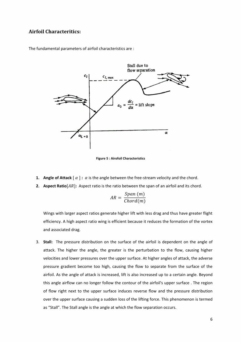
Airfoil Characteritics:
The fundamental parameters of airfoil characteristics are :
Figure 5 : Airofoil Characteristics
1. Angle of Attack : is the angle between the free-stream velocity and the chord.
2. Aspect Ratio : Aspect ratio is the ratio between the span of an airfoil and its chord.
Wings with larger aspect ratios generate higher lift with less drag and thus have greater flight
efficiency. A high aspect ratio wing is efficient because it reduces the formation of the vortex
and associated drag.
3. Stall: The pressure distribution on the surface of the airfoil is dependent on the angle of
attack. The higher the angle, the greater is the perturbation to the flow, causing higher
velocities and lower pressures over the upper surface. At higher angles of attack, the adverse
pressure gradient become too high, causing the flow to separate from the surface of the
airfoil. As the angle of attack is increased, lift is also increased up to a certain angle. Beyond
this angle airflow can no longer follow the contour of the airfoil's upper surface . The region
of flow right next to the upper surface induces reverse flow and the pressure distribution
over the upper surface causing a sudden loss of the lifting force. This phenomenon is termed
as “Stall”. The Stall angle is the angle at which the flow separation occurs.

7
Finite Element Method (FEM)
The finite element method (FEM) is a computational technique used to obtain approximate
solutions of boundary value problems in engineering. FEM is used for problems with
complicated geometries, loadings, and material properties where analytical solutions cannot
be obtained.
Figure 6 : Idea of FEM
Basic laws of nature are typically expressed in the form of partial differential equations
(PDE), such as Navier-Stokes equations of fluid flow. The Finite element method has
emerged as a universal tool for the computational solution of PDEs with a multitude of
applications in engineering and science. Adaptivity is an important computational
technology where the FEM algorithm is automatically tailored to compute a user specified
output of interest to a chosen accuracy, to a minimal computational cost.
Figure 7 : Finite Element Process

8
In the Finite Element Method (FEM) we approximate the exact solution function “ ” as a
piecewise polynomial and compute co-efficients by enforcing orthogonality (Galerkin’s
Method) [13] [14] [15].
The basic steps involved in FEM are explained as below [18] :
Figure 8 : Finite Element Domain
Polynomial Approximation:
We seek polynomial approximations “ ” to “ ”. A vector space can be constructed with a
set of polynomials on a domain as basis vectors, where function addition and scalar
multiplication satisfy the requirements for a vector space.
We can also define an inner product space with the inner product defined as:
The inner product generates the norm:
Just like in we define orthogonality between two vectors as :

9
The Cauchy-Schwartz inequality is given by:
Polynomial vector space consists of polynomials:
One basis is the monomials:
Piecewise linear polynomials:
Global polynomials on the whole domain led to vector space (monomials basis:
). Only way of refining approximate solution is by increasing . We instead
look at piecewise polynomials.
Partition domain into mesh: by placing
nodes . We define polynomial function on each subinterval with length
Figure 9 : Global basis "tent" function

10
Nodal Basis:
Basis function:
Vector Space of continuous piecewise linear polynomials: with basis , number of
nodes in mesh.
Figure 10 : Piecewise linear polynomials
Piecewise linear function:
We define the residual function for a differential equation as :
,
We can thus define an equation with exact solution as:

11
Galerkin’s method:
We seek a solution in finite element vector space of the form:
We require the residual to be orthogonal to :
This form is also known as the ”Weak formulation”.
For terms in with two derivatives we perform integration by parts to move one
derivative to the test function.
In a nutshell the Mathematical Model Formulation for our case is described as below:
Method – PDE For a given differential equation,
Function Space and Discrete function Space,
Weak form of the PDE is given by:
Numerical Approximation The Finite Element Method is defined by:
Where Discrete Space,

12
Numerical Approximation applied to Fluid flow
Refer Eq. (i) in page no.23 and Eq. (ii) in page no.27
Error Estimation We follow the general framework for a posteriori error estimation based on the solution of
associated dual problems.
We use an A Posteriori Error Estimate , where is the error and is an output functional of interest.
Residual:
Primal Problem:
Dual Problem: A Posteriori Error Estimate can be re-written as:
Further estimates (see [4]) results in the following Error Indicator:

13
Adaptive Algorithm
In practice, the dual solution is approximated by a similar finite element method as we use
for the primal problem, linearized at the primal solution. Based on the a posteriori error
indicator we can then form adaptive algorithms for how to construct finite element meshes
optimized to approximate the functional.
Starting from an initial coarse mesh , one simple such algorithm implemented in Unicorn
takes the form: let k = 0 then do :
Adaptive mesh refinement Algorithm
1. For the mesh compute the primal problem and the dual problem.
2. If then stop, else:
3. Mark some chosen percentage of the elements with highest for refinement
4. Generate the refined mesh , set k = k+1, and go to 1.

14
3. NACA Airfoil
During the initial stage of our project, we had to choose a wing suitable for project
specifications. A wing having high aspect ratio (HR = 5), Reynolds number of range (Re) 10^6
– 10^7, published data and geometry modifications are permitted. NTNU had two wings
prototypes at their inventory. Considering our project specifications, NTNU proposed two
wing prototypes:
1. “Stratford” wing, developed at NTNU and Confidential (Re= ~ 0.8M). As it was a
custom wing developed at NTNU, we were not allowed to do any geometry
modifications.
2. “NACA64 (2)-415” wing - high aspect ratio standard wing (Re= ~ 0.5M). We were
allowed to make the geometry modifications.
The specifications of the NACA wing were in-line with our project specifications. Based on
the cost estimation, time limitations and the specifications, we decided to use the “NACA64
(2)-415 wing”, for our project.
Nomenclature
Figure 11 : Cambered Airfoil Geometry
The figure above shows the key terms used in nomenclature of the Airfoil Geometry. The
mean camber line is defined to lie halfway between the upper and lower surface

15
Where,
- stands for National Advisory Committee for Aeronautics
- denotes the Series designation
- denotes the chordwise position of minimum pressure in tenths of the chord
behind the leading edge for the basic symmetrical section at zero lift
- The subscript indicates the range of lift coefficient in tenths above and below the
design lift coefficient in which favourable pressure gradient exist on both surfaces
- following the dash denotes the design lift coefficient in tenths
- The final two digits denotes airfoil thickness in percent of the chord (15%)
The Cambered airfoil sections of all NACA families considered herein are obtained by
combining a mean line and a thickness distribution [16] [17].
Figure 12 : NACA Airfoil co-ordinates
The abscissas, ordinates and slopes of the mean line are designated as , and
respectively. If and represent the abscissa and ordinate of a typical point of the
Upper surface of the airfoil and is the ordinate of the symmetrical thickness distribution
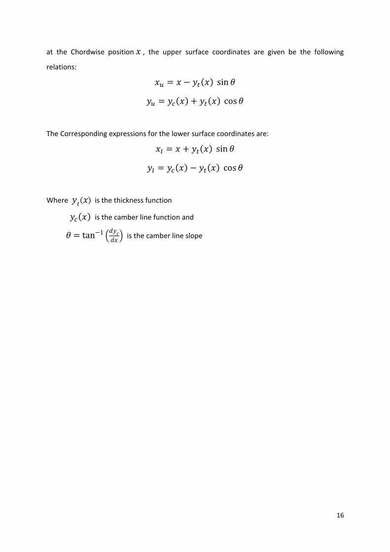
16
at the Chordwise position , the upper surface coordinates are given be the following
relations:
The Corresponding expressions for the lower surface coordinates are:
Where is the thickness function
is the camber line function and
is the camber line slope

17
4. Numerical Investigation
4.1. Governing Equations
In fluid mechanics, flow of air at subsonic speed is captured by the incompressible navier-
stokes equations with the Reynolds number ( ) as an important flow characteristic,
Where: is a characteristic flow speed
is a characteristic length scale
is the kinematic viscosity [For water and for air ]
The basic mathematical model for a flight simulation consists of Navier-Stokes equations
expressing conservation of mass, momentum and energy of a viscous fluid. The
incompressible Navier-Stokes equations thus can be viewed to consist of two equations in
the fluid velocity and pressure expressing
- Newton’s 2nd Law (conservation of momentum)
- Incompressibility.
As a basic model we use the Incompressible Navier-Stokes Equations for Velocity and
Pressure:
.............................. (i)
with the kinematic viscosity.
NOTE: Flight at speeds up to 300 km/h (83.33 m/s) of airplanes is described by solutions of the incompressible
Navier-Stokes equations at a Reynolds number of size or larger, which with normalization to
translate to small viscosity of size or smaller. Typically for flows with Mach number below 0.2 - 0.3 can be
modeled as incompressible
18
4.2. Computing Lift and Drag Coefficients
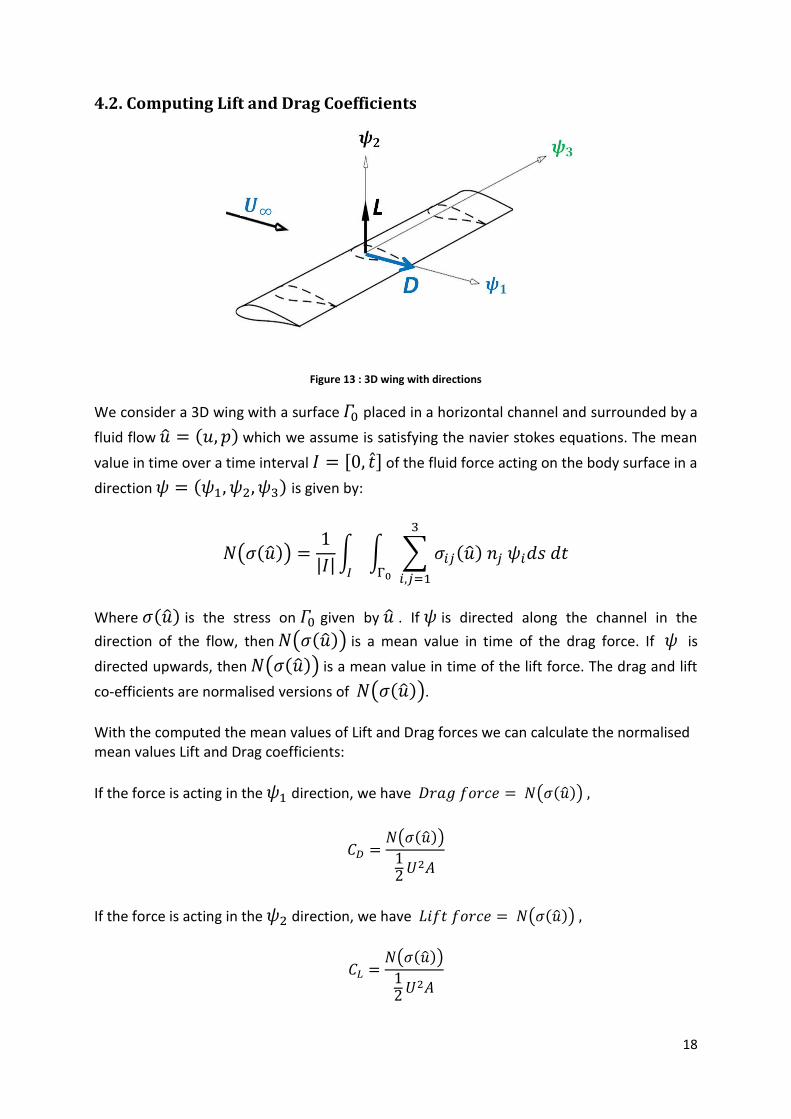
Figure 13 : 3D wing with directions
We consider a 3D wing with a surface placed in a horizontal channel and surrounded by a
fluid flow which we assume is satisfying the navier stokes equations. The mean
value in time over a time interval of the fluid force acting on the body surface in a
direction is given by:
Where is the stress on given by . If is directed along the channel in the
direction of the flow, then is a mean value in time of the drag force. If is
directed upwards, then is a mean value in time of the lift force. The drag and lift
co-efficients are normalised versions of .
With the computed the mean values of Lift and Drag forces we can calculate the normalised mean values Lift and Drag coefficients:
If the force is acting in the direction, we have
If the force is acting in the direction, we have

19
4.2. Boundary Conditions for the Numerical Method
The Navier-Stokes equations in the fluid domain are complemented by boundary conditions
on the boundary of the fluid domain prescribing velocities or forces or combinations. We will
be considering the “Slip” normal velocity and tangential forces are put to zero. [13]
We model the turbulent boundary layer by a slip with friction boundary condition which can
be written:
with an outward unit normal vector, and orthogonal unit tangent vectors at the
boundary. Here can be chosen as a constant parameter, or as a function of space and
time, similar to simple wall shear stress models. For very high Reynolds numbers we find
that is a good approximation for small skin friction stress, which have been validated
for a number of benchmark problems [13] .
According to Johan Hoffman, Johan Jansson, Niclas Jansson [13] ”The slip boundary
condition is implemented in strong form, where the boundary condition is applied after
assembling the left-hand side matrix and the right-hand side vector modifying the algebraic
system, whereas the tangential components are implemented in weak form by adding
boundary integrals in the variational formulation.
The node normals are computed from a weighted average of the surrounding facet normals.
Edges and corners are identified from the angles between facet normals, for which the
velocity is constrained in 2 and 3 linearly independent directions respectively”.
We need to be careful when constucting the mesh near rounded surfaces of sharp radius, to
avoid artificially constraining velocities.
20
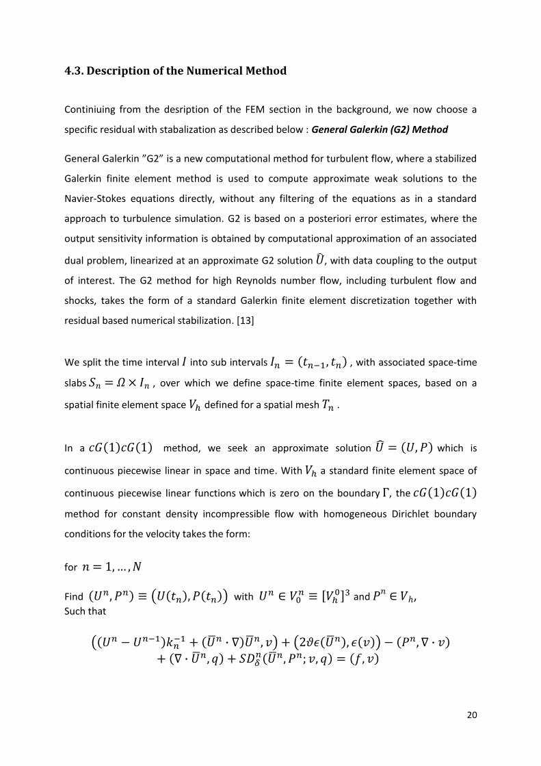
4.3. Description of the Numerical Method
Continiuing from the desription of the FEM section in the background, we now choose a
specific residual with stabalization as described below : General Galerkin (G2) Method
General Galerkin ”G2” is a new computational method for turbulent flow, where a stabilized
Galerkin finite element method is used to compute approximate weak solutions to the
Navier-Stokes equations directly, without any filtering of the equations as in a standard
approach to turbulence simulation. G2 is based on a posteriori error estimates, where the
output sensitivity information is obtained by computational approximation of an associated
dual problem, linearized at an approximate G2 solution , with data coupling to the output
of interest. The G2 method for high Reynolds number flow, including turbulent flow and
shocks, takes the form of a standard Galerkin finite element discretization together with
residual based numerical stabilization. [13]
We split the time interval into sub intervals , with associated space-time
slabs , over which we define space-time finite element spaces, based on a
spatial finite element space defined for a spatial mesh .
In a method, we seek an approximate solution which is
continuous piecewise linear in space and time. With a standard finite element space of
continuous piecewise linear functions which is zero on the boundary , the
method for constant density incompressible flow with homogeneous Dirichlet boundary
conditions for the velocity takes the form:
for
Find with
and , Such that

21
Where: is piecewise constant in time over , with the
stabilizing term,
.............................. (ii)
Where we have dropped the shock capturing term and where
with the stabilization parameters
where and are positive constants of unit size.
For turbulent flow, the time step size is
The least squares stabilization omits the time derivative in the residual, which is a
consequence of the test functions being piecewise constant in time for discretization
of time.

22
4.4. Software Environment
The software environment shows the interdepencencey of each software at different stages
of the simulations.
Figure 14 : Overview of the Software Environment
SolidWorks
The SolidWorks® CAD software is a mechanical design automation application that lets
designers quickly sketch out ideas, experiment with features and dimensions, and produce
models and detailed drawings.
NETGEN
NETGEN is an automatic 3d tetrahedral mesh generator. It accepts input from constructive
solid geometry (CSG) or boundary representation (BRep) from STL file format. The
connection to a geometry kernel allows the handling of IGES and STEP files. NETGEN
contains modules for mesh optimization and hierarchical mesh refinement. Netgen is open
source based on the LGPL license. It is available for Unix/Linux and Windows.
23
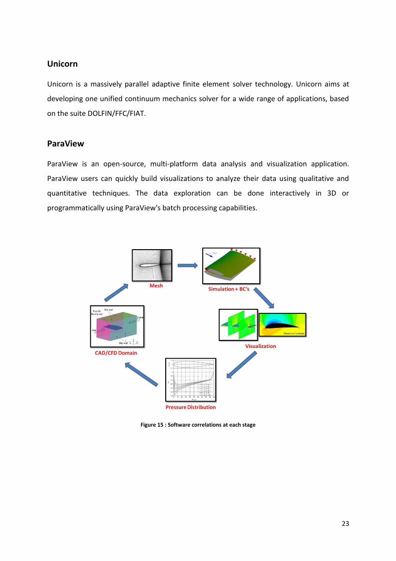
Unicorn Unicorn is a massively parallel adaptive finite element solver technology. Unicorn aims at
developing one unified continuum mechanics solver for a wide range of applications, based
on the suite DOLFIN/FFC/FIAT.
ParaView ParaView is an open-source, multi-platform data analysis and visualization application.
ParaView users can quickly build visualizations to analyze their data using qualitative and
quantitative techniques. The data exploration can be done interactively in 3D or
programmatically using ParaView's batch processing capabilities.
Figure 15 : Software correlations at each stage

24
4.5. Geometry Modelling
The CAD model of the NACA 64(2)-415 section airfoil with 242 mm chord and 1200 mm span
were generated as the dimensions relative to the prototype. The 3D wing model and the
computational domain is generated by using SolidWorks® CAD software [19].
Figure 16 : 3D CAD modelling of the NACA Wing
Two variants were considered for the investigation ”clean wing” and ”protrusion wing”.
Clean wing is the standard wing and the protrusion wing is standard wing with a geometry
modification (semi circular boss near the leading egde). The semi-circular protrusion is
located at the 8% of the chord length.
Figure 17 : Clean Wing and Protruson Wing CAD Models
25
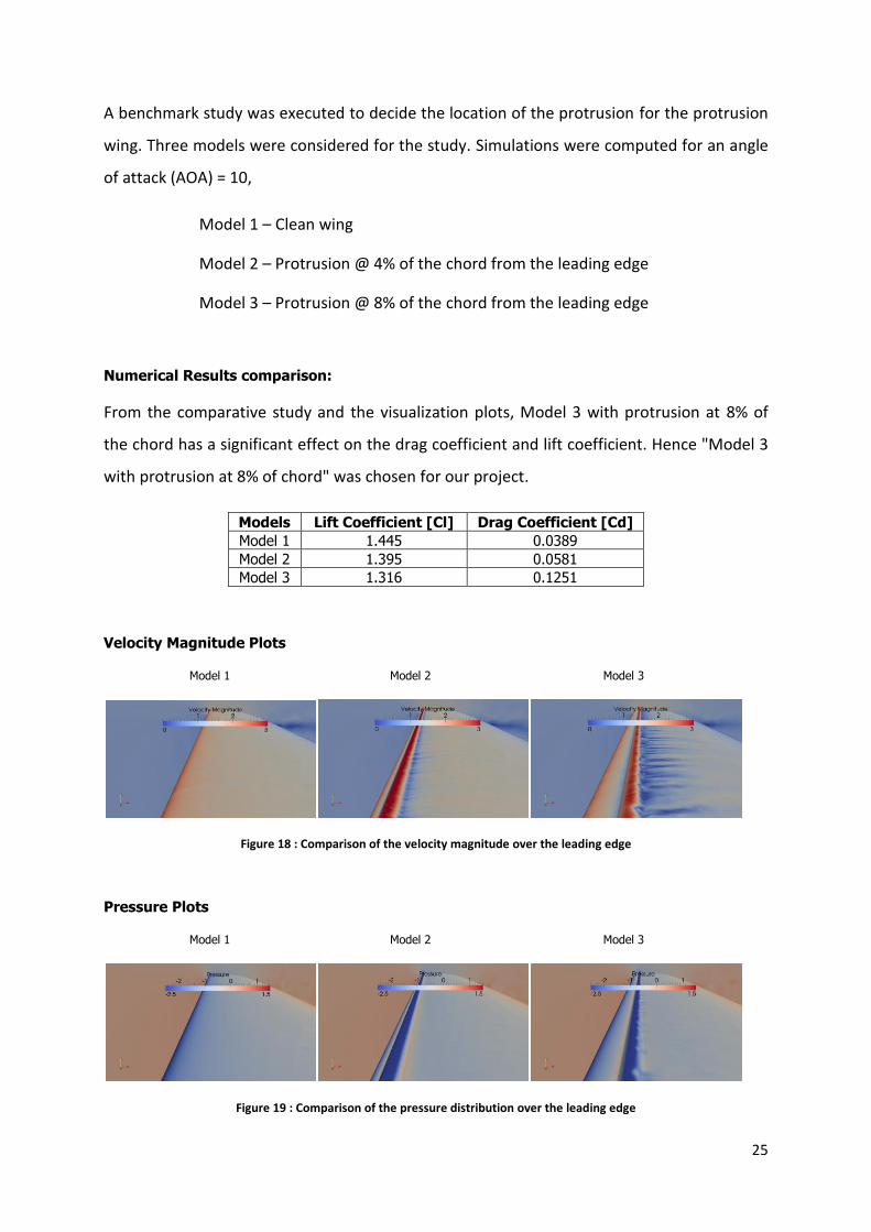
A benchmark study was executed to decide the location of the protrusion for the protrusion
wing. Three models were considered for the study. Simulations were computed for an angle
of attack (AOA) = 10,
Model 1 – Clean wing
Model 2 – Protrusion @ 4% of the chord from the leading edge
Model 3 – Protrusion @ 8% of the chord from the leading edge
Numerical Results comparison:
From the comparative study and the visualization plots, Model 3 with protrusion at 8% of
the chord has a significant effect on the drag coefficient and lift coefficient. Hence "Model 3
with protrusion at 8% of chord" was chosen for our project.
Models Lift Coefficient [Cl] Drag Coefficient [Cd]
Model 1 1.445 0.0389
Model 2 1.395 0.0581
Model 3 1.316 0.1251
Velocity Magnitude Plots
Model 1 Model 2 Model 3
Figure 18 : Comparison of the velocity magnitude over the leading edge
Pressure Plots
Model 1 Model 2 Model 3
Figure 19 : Comparison of the pressure distribution over the leading edge
26
4.6. Mesh Generation
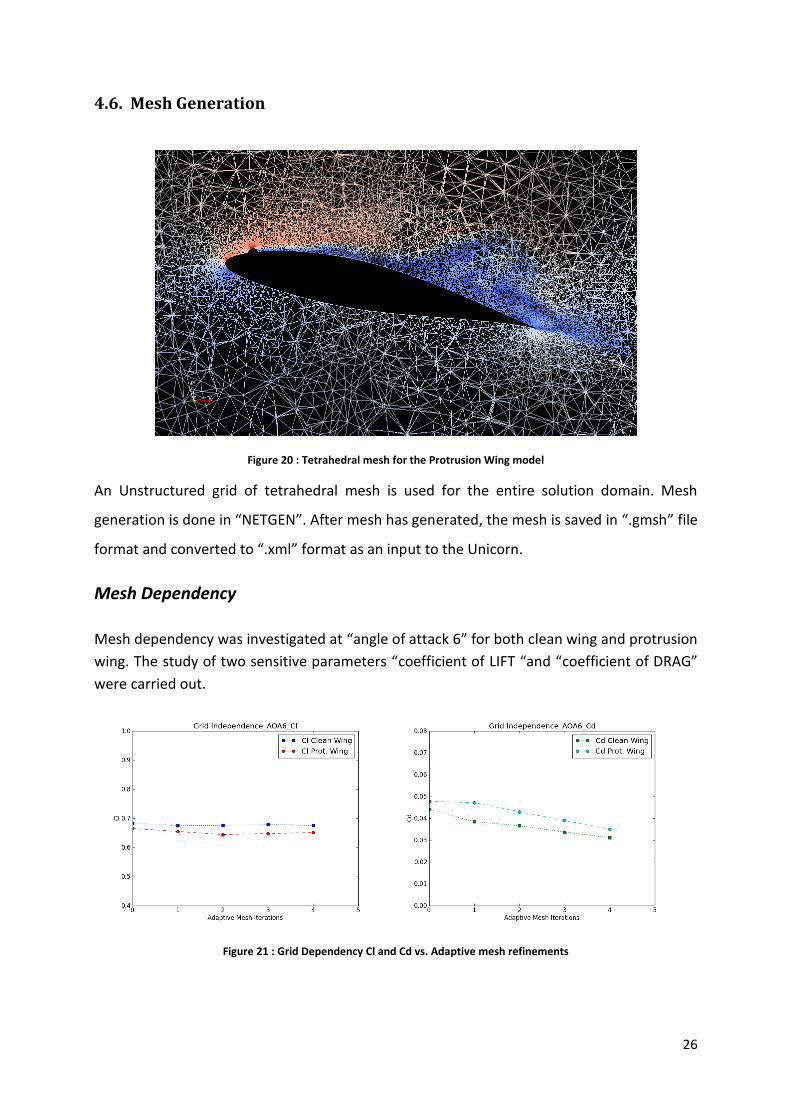
Figure 20 : Tetrahedral mesh for the Protrusion Wing model
An Unstructured grid of tetrahedral mesh is used for the entire solution domain. Mesh
generation is done in “NETGEN”. After mesh has generated, the mesh is saved in “.gmsh” file
format and converted to “.xml” format as an input to the Unicorn.
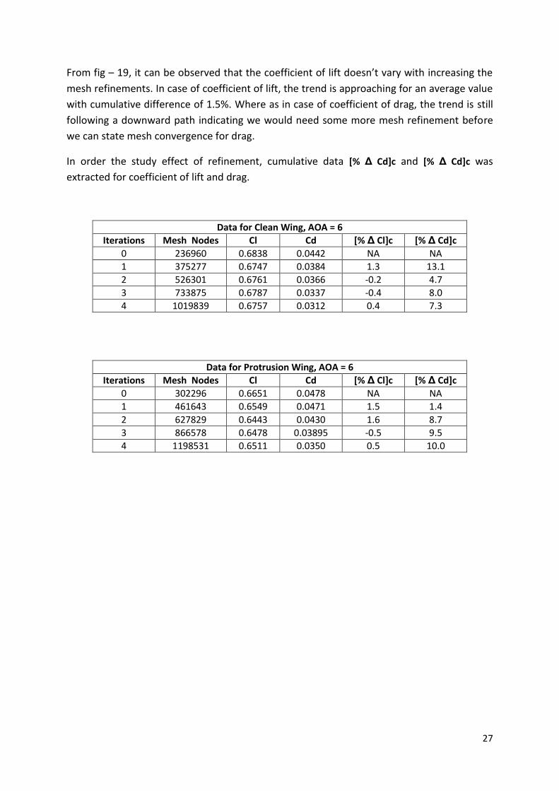
Mesh Dependency
Mesh dependency was investigated at “angle of attack 6” for both clean wing and protrusion
wing. The study of two sensitive parameters “coefficient of LIFT “and “coefficient of DRAG”
were carried out.
Figure 21 : Grid Dependency Cl and Cd vs. Adaptive mesh refinements
27
From fig – 19, it can be observed that the coefficient of lift doesn’t vary with increasing the
mesh refinements. In case of coefficient of lift, the trend is approaching for an average value
with cumulative difference of 1.5%. Where as in case of coefficient of drag, the trend is still
following a downward path indicating we would need some more mesh refinement before
we can state mesh convergence for drag.
In order the study effect of refinement, cumulative data [% Δ Cd]c and [% Δ Cd]c was
extracted for coefficient of lift and drag.
Data for Clean Wing, AOA = 6
Iterations Mesh Nodes Cl Cd [% Δ Cl]c [% Δ Cd]c
0 236960 0.6838 0.0442 NA NA
1 375277 0.6747 0.0384 1.3 13.1
2 526301 0.6761 0.0366 -0.2 4.7
3 733875 0.6787 0.0337 -0.4 8.0
4 1019839 0.6757 0.0312 0.4 7.3
Data for Protrusion Wing, AOA = 6
Iterations Mesh Nodes Cl Cd [% Δ Cl]c [% Δ Cd]c
0 302296 0.6651 0.0478 NA NA
1 461643 0.6549 0.0471 1.5 1.4
2 627829 0.6443 0.0430 1.6 8.7
3 866578 0.6478 0.03895 -0.5 9.5
4 1198531 0.6511 0.0350 0.5 10.0
28
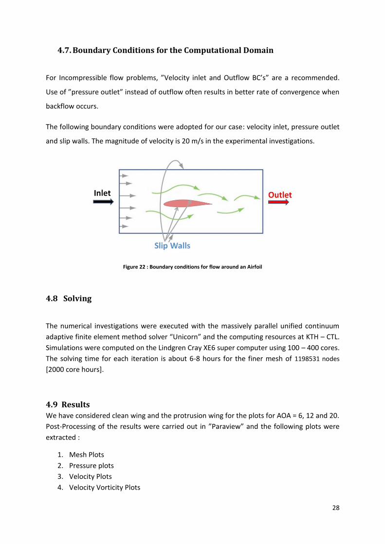
4.7. Boundary Conditions for the Computational Domain
For Incompressible flow problems, ”Velocity inlet and Outflow BC’s” are a recommended.
Use of ”pressure outlet” instead of outflow often results in better rate of convergence when
backflow occurs.
The following boundary conditions were adopted for our case: velocity inlet, pressure outlet
and slip walls. The magnitude of velocity is 20 m/s in the experimental investigations.
Figure 22 : Boundary conditions for flow around an Airfoil
4.8 Solving
The numerical investigations were executed with the massively parallel unified continuum
adaptive finite element method solver “Unicorn” and the computing resources at KTH – CTL.
Simulations were computed on the Lindgren Cray XE6 super computer using 100 – 400 cores.
The solving time for each iteration is about 6-8 hours for the finer mesh of 1198531 nodes
[2000 core hours].
4.9 Results
We have considered clean wing and the protrusion wing for the plots for AOA = 6, 12 and 20.
Post-Processing of the results were carried out in ”Paraview” and the following plots were
extracted :
1. Mesh Plots
2. Pressure plots
3. Velocity Plots
4. Velocity Vorticity Plots

29
Mesh Plots
Three dimensional unstructured tetrahedral meshes were generated using an adaptive mesh
algorithm.The mesh distribution over the wings are visualized in Paraview. From the
following mesh plots we can observe that finer mesh are around boundary of the airfoil and
coarse meshes are in the outer region.
AOA = 6
AOA = 12
AOA = 20
Figure 23 : Mesh plots at different AOA for Clean (Left) and Protrusion Wing (Right)

30
2D Pressure Plots
Fig. 24 shows the comparison of the pressure distribution for clean wing and protrusion wing
for angle of attacks (AOA) 6, 12 and 20.
AOA = 06
AOA = 12
AOA = 20
Figure 24 : 2D Pressure plots at different AOA for Clean wing (Left) and Protrusion Wing (Right)
31
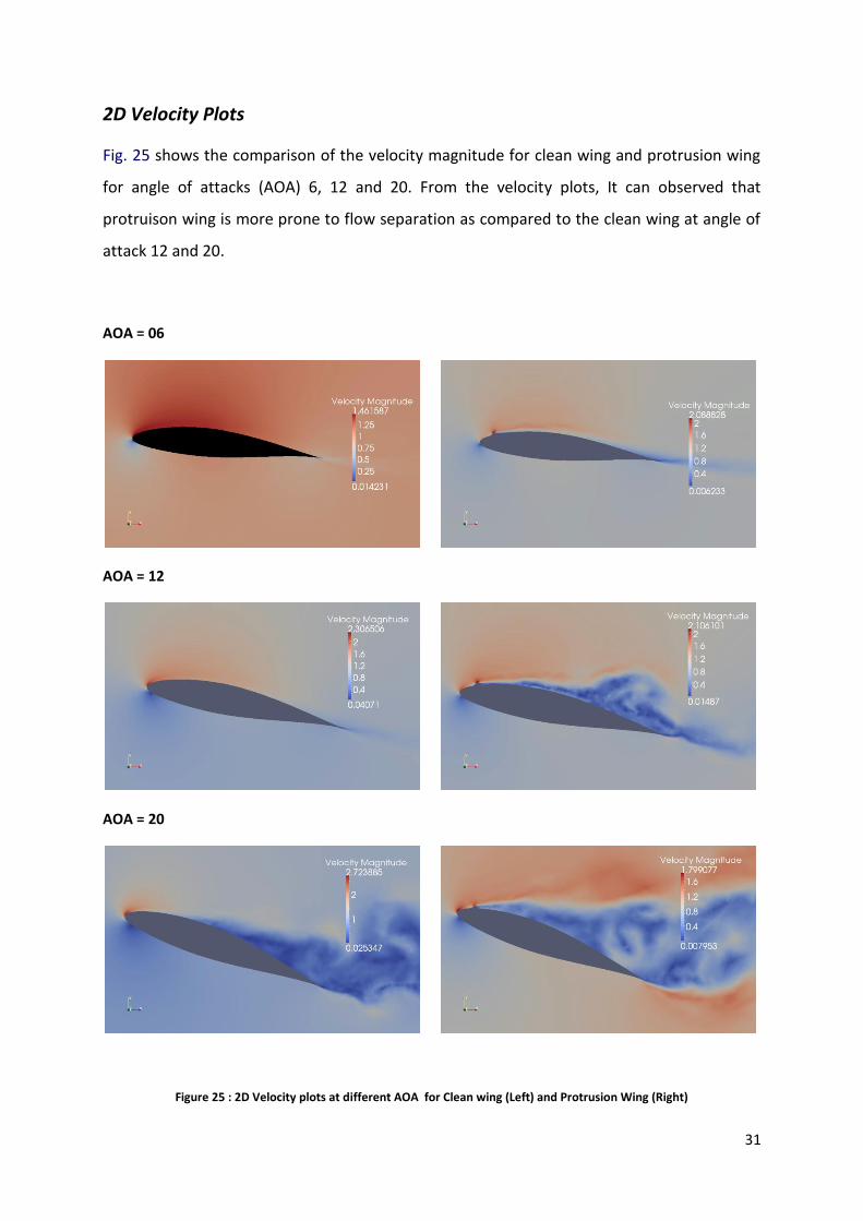
2D Velocity Plots
Fig. 25 shows the comparison of the velocity magnitude for clean wing and protrusion wing
for angle of attacks (AOA) 6, 12 and 20. From the velocity plots, It can observed that
protruison wing is more prone to flow separation as compared to the clean wing at angle of
attack 12 and 20.
AOA = 06
AOA = 12
AOA = 20
Figure 25 : 2D Velocity plots at different AOA for Clean wing (Left) and Protrusion Wing (Right)
32
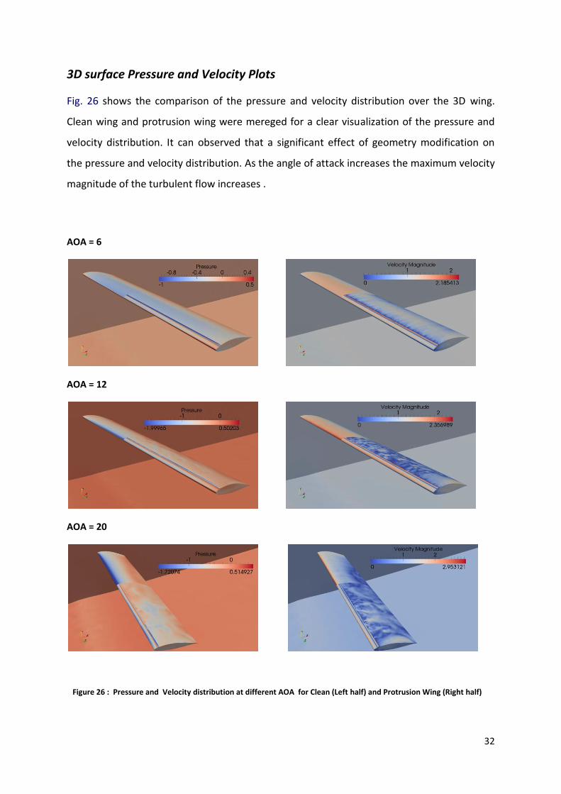
3D surface Pressure and Velocity Plots
Fig. 26 shows the comparison of the pressure and velocity distribution over the 3D wing.
Clean wing and protrusion wing were mereged for a clear visualization of the pressure and
velocity distribution. It can observed that a significant effect of geometry modification on
the pressure and velocity distribution. As the angle of attack increases the maximum velocity
magnitude of the turbulent flow increases .
AOA = 6
AOA = 12
AOA = 20
Figure 26 : Pressure and Velocity distribution at different AOA for Clean (Left half) and Protrusion Wing (Right half)

33
Velocity Vorticity Plots
The velocity vorticity plots over the wings are one critical parameter to study in a
aerodynamic simulations. From the following plots we can observe that protrusion wing
model has higher tendency for the vorticities as compared to the clean wing.
AOA = 6
AOA = 12
AOA = 20
Figure 27 : Velocity Vorticity plots at different AOA for Clean (Left) and Protrusion Wing (Right)

34
5. Experimental Investigation
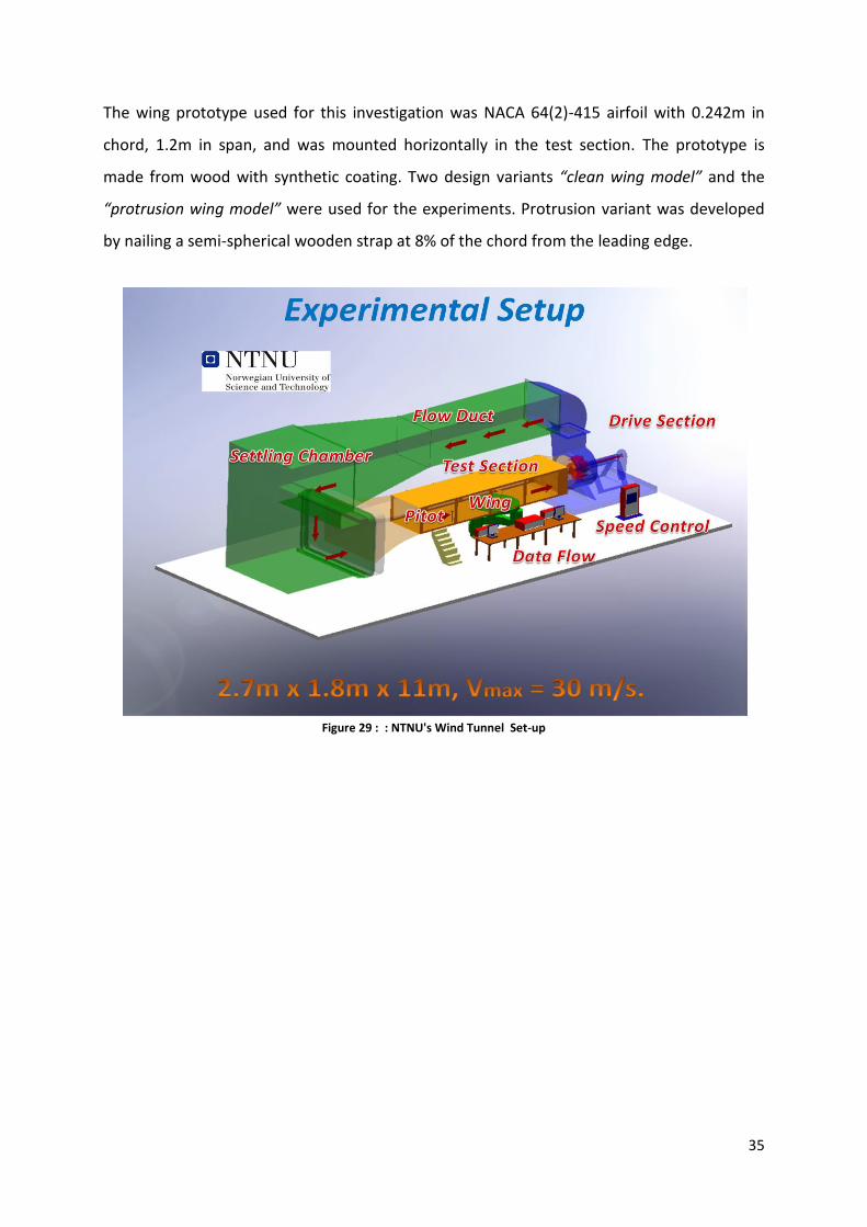
5.1. Description of the Experimental Setup
Experiments were carried out in the low speed wind tunnel of the Norwegian University of
Science and Technology (NTNU), Trondheim.
Figure 28 : NTNU's Wind Tunnel
The wind tunnel is a closed-return wind-tunnel that is principally used for three-dimensional
testing. A heat exchanger, honeycomb and three turbulence reduction screens are located at
the inlet settling chamber. The test section dimensions are 2.7m x 1.8m x 11m and maximum
velocity of 30 m/s. Desired airspeed is achieved using a variable frequency drive. Fig. 27
shows a picture of the wind tunnel facilities.
35
The wing prototype used for this investigation was NACA 64(2)-415 airfoil with 0.242m in
chord, 1.2m in span, and was mounted horizontally in the test section. The prototype is
made from wood with synthetic coating. Two design variants “clean wing model” and the
“protrusion wing model” were used for the experiments. Protrusion variant was developed
by nailing a semi-spherical wooden strap at 8% of the chord from the leading edge.
Figure 29 : : NTNU's Wind Tunnel Set-up
36
5.2. Measurements
A high resolution 6 component electronic wind tunnel balance is used for the velocity –
pressure - force measurements. A large number of high speed 12 bit data acquisition with
signal conditioning amplifiers and filters are available capable of recording data continuously
to disk at a rate up to 1 MHz.
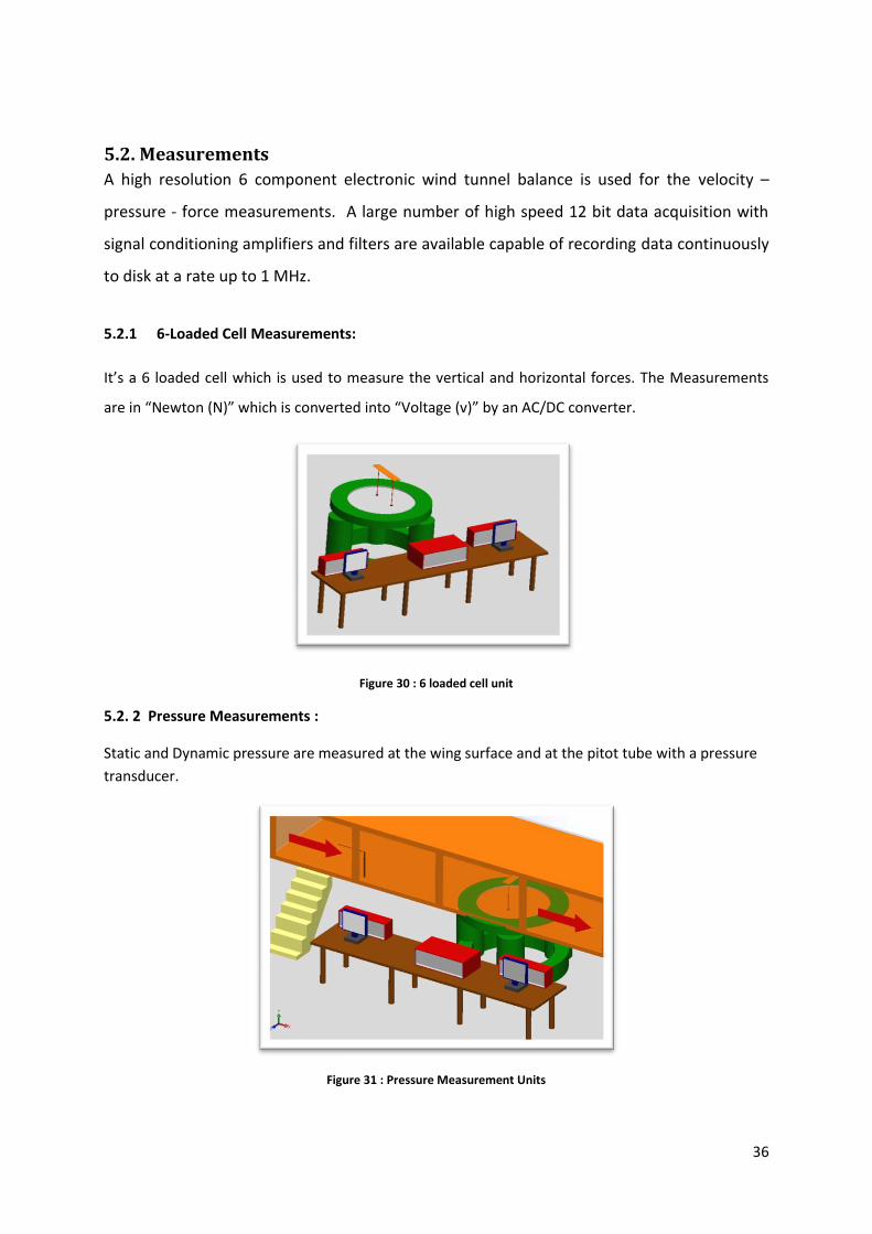
5.2.1 6-Loaded Cell Measurements:
It’s a 6 loaded cell which is used to measure the vertical and horizontal forces. The Measurements
are in “Newton (N)” which is converted into “Voltage (v)” by an AC/DC converter.
Figure 30 : 6 loaded cell unit
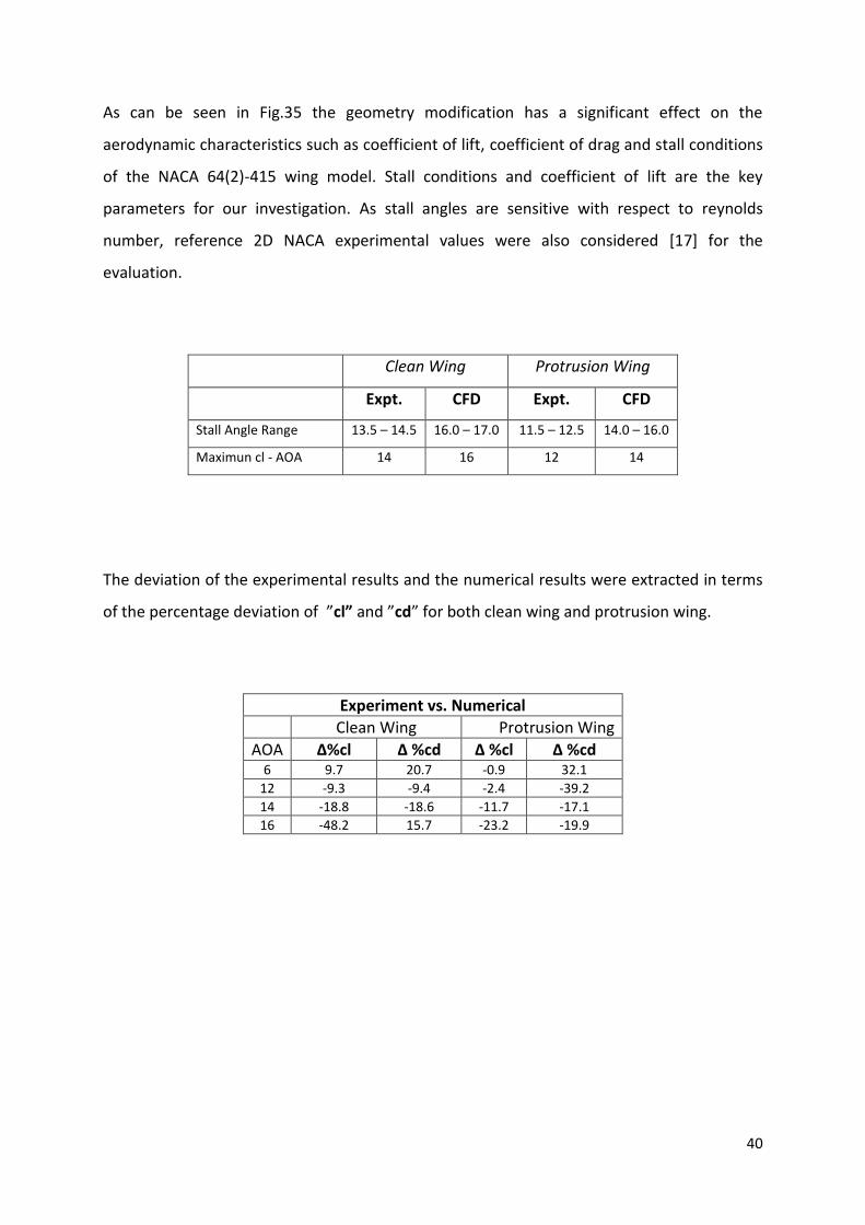
5.2. 2 Pressure Measurements :
Static and Dynamic pressure are measured at the wing surface and at the pitot tube with a pressure
transducer.
Figure 31 : Pressure Measurement Units

37
Pressure taps were mounted on the upper and lower surfaces of the wing. The pressure taps are
connected to the pressure inducer and the measuring units.
Figure 32 : Pressure Transducer and Data flow of from the Pressure Taps on the wing
5.2. 3 Angle of Attack [AOA] Measurement
Angle measurements were carried out manually with a digital protractor and a custom made
level made from wood.
Figure 33 : Tools for the Angle of Attack Measurements

38
5.2. 4 TUFTS Visualization
TUFTS visualization is carried out by attaching 50 - 60 thread TUFTS of four rows on to the
upper surface of the wing model. When the wind is turned on the tufts move in the direction
of the flow. Flow visulaizations were carried out for number of angles from stagnation still
stall.
Figure 34 : Threaded TUFT Visualization of the Protrusion Wing Model
5. stigation

39
6. Results Comparison and Discussion
The aerodynamic performance characteristics of the NACA 64(2)-415 wing are presented
for the two design variants ”clean wing” and the ”protrusion wing”. The experimental
and numerical solutions were compared to investigate the effect of the geometry
modification on the aerodynamic characteristics and to measure the deviation.
Description Reynolds Number Wing Tip
NTNU Experiment (3D) 3.2 x Filleted Wing tip edges
NACA Experiment (2D) 3.1 x Free wing tip
Numerical Simulation (3D) Higher (≈ ∞) Filleted Wing tip edges
Figure 35 : Performance Evaluation
40
As can be seen in Fig.35 the geometry modification has a significant effect on the
aerodynamic characteristics such as coefficient of lift, coefficient of drag and stall conditions
of the NACA 64(2)-415 wing model. Stall conditions and coefficient of lift are the key
parameters for our investigation. As stall angles are sensitive with respect to reynolds
number, reference 2D NACA experimental values were also considered [17] for the
evaluation.
Clean Wing Protrusion Wing
Expt. CFD Expt. CFD
Stall Angle Range 13.5 – 14.5 16.0 – 17.0 11.5 – 12.5 14.0 – 16.0
Maximun cl - AOA 14 16 12 14
The deviation of the experimental results and the numerical results were extracted in terms
of the percentage deviation of ”cl” and ”cd” for both clean wing and protrusion wing.
Experiment vs. Numerical Clean Wing Protrusion Wing
AOA Δ%cl Δ %cd Δ %cl Δ %cd 6 9.7 20.7 -0.9 32.1
12 -9.3 -9.4 -2.4 -39.2
14 -18.8 -18.6 -11.7 -17.1
16 -48.2 15.7 -23.2 -19.9
41
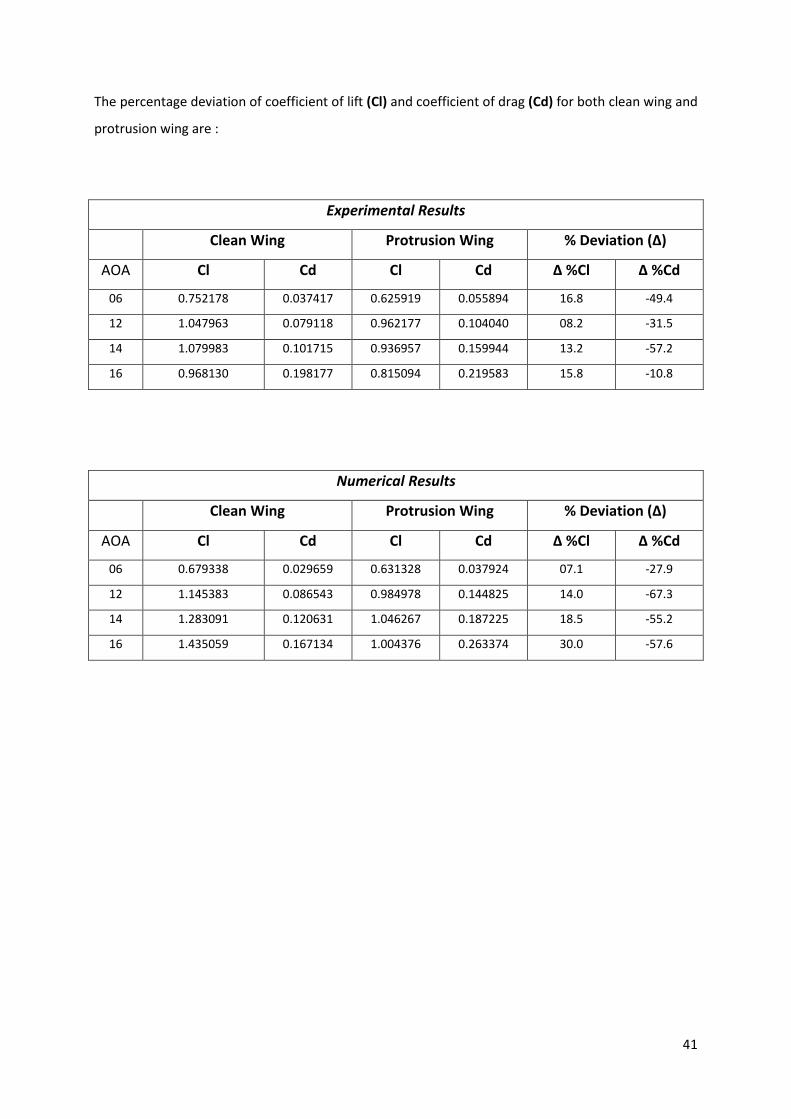
The percentage deviation of coefficient of lift (Cl) and coefficient of drag (Cd) for both clean wing and
protrusion wing are :
Experimental Results
Clean Wing Protrusion Wing % Deviation (Δ)
AOA Cl Cd Cl Cd Δ %Cl Δ %Cd
06 0.752178 0.037417 0.625919 0.055894 16.8 -49.4
12 1.047963 0.079118 0.962177 0.104040 08.2 -31.5
14 1.079983 0.101715 0.936957 0.159944 13.2 -57.2
16 0.968130 0.198177 0.815094 0.219583 15.8 -10.8
Numerical Results
Clean Wing Protrusion Wing % Deviation (Δ)
AOA Cl Cd Cl Cd Δ %Cl Δ %Cd
06 0.679338 0.029659 0.631328 0.037924 07.1 -27.9
12 1.145383 0.086543 0.984978 0.144825 14.0 -67.3
14 1.283091 0.120631 1.046267 0.187225 18.5 -55.2
16 1.435059 0.167134 1.004376 0.263374 30.0 -57.6
42
7. Conclusions
The experimental and numerical investigations have been performed for two cases
(Clean wing and Protrusion wing) of the NACA 64(2)415 wing. The numerical
investigation was executed with the massively parallel unified continuum adaptive finite
element method solver ”Unicorn”. The accuracy of the numerical results has been
validated against the experimental results. The results comparison show that the
deviation between the experimental and numerical results is small for the lower angles
of attack and gradually increases for higher angles of attack. The study also shows that
the protrusion wing resulted in a lower lift and higher drag as compared to the clean
wing.
Our investigation leads to the following conclusions :
1. The experimental and numerical results have good correlations for lower
range of angle of attack (6°–12°) before stall angle. The average percentage
difference compared to experiment is less than 10 % for coefficient of lift and
less than 30 % for coefficient of drag. The errors are within the acceptable
range, compared to the previous research [6, 13] which is a positive outcome
of the project.
2. The percentage difference after the stall angle is large. The main reason for
this large difference in the clean wing is due to the difference in the reynolds
number , which in turn has a large effect on the stall angle. The reynolds
number considered for experiment investigation is , where as for
numerical investigations is considered to be high
.
3. The numerical results of the clean wing have a close relevance with the
reference NACA published results. Especially the stall angle for the clean wing
and reference NACA values are in a range of 16°–17°. From the reference

43
NACA published results we can conclude that stall angles are sensitive to the
reynolds number .
4. Protrusion wing model resulted in lower lift, higher drag and earlier stall as
compared to the clean wing model. The average percentage reduction in lift is
ca. 15 % and increase in drag 40 – 50 %, both in experiments and simulations.
5. From the mesh convergence study, we can summarize that the average
percentage variation of coefficient of lift is less than 5 % with respect to the
last 5 adaptive iterations. The results comparison was done with the
consecutive adaptive mesh iterations.
6. Additional experimental investigations for the new designs would leads to
additional cost, so in this scenario numerical simulations would be a cost
effective solution.
8. Scope for future work
Our research and results presented in this thesis provide valuable insight to understand
the effect of geometry modification on the aerodynamic characteristics of a wing and
overview of Unicorn framework .
The following scope for future work were identified :
1. To get a better understanding of the effect of protrusion an in-depth pressure
distribution study over the Clean and Protrusion wings are required.
2. In order to expand the horizon of the project, numerical investigations for “Dented”
and “Leading Edge Tubercles” case studies would be a new area of interest.
44
9. References
[1] P. Moin, J. Kim, Tackling turbulence with supercomputers, Scientific American, 1997.
[2] P. Moin, D. You, Active control of flow separation over an airfoil using synthetic jets, Journal of
Fluids and Structures 24, 2008
[3] P. Sagaut, Large Eddy Simulation for Incompressible Flows (3rd Ed.), Springer-Verlag, Berlin,
Heidelberg, New York, 2005
[4] J. Hoffman, C. Johnson, Computational Turbulent Incompressible Flow, Vol. 4 of Applied
Mathematics: Body and Soul, Springer, 2007.
[5] J. Hoffman, J. Jansson, C. Degirmenci, N. Jansson, M. Nazarov, Unicorn: A Unified Continuum
Mechanics Solver, in: Automated Scientific Computing, Springer, 2011
[6] J. Hoffman, Computation of mean drag for bluff body problems using adaptive dns/les, SIAM J.
Sci. Comput. 27(1) (2005) 184–207
[7] J. Hoffman, J. Jansson, C. Degirmenci, N. Jansson, M. Nazarov, Unicorn: A Unified Continuum
Mechanics Solver, in: Automated Scientific Computing, Springer, 2011
[8] J. Hoffman, Adaptive simulation of the subcritical flow past a sphere, J. Fluid Mech. 568 (2006)
77–88.
[9] J. Hoffman, Efficient computation of mean drag for the subcritical flow past a circular cylinder
using general Galerkin G2, Int. J. Numer. Meth. Fl. 59 (11) (2009) 1241–1258
[10] J. Hoffman, N. Jansson, A computational study of turbulent flow separation for a circular
cylinder using skin friction boundary conditions, in: Quality and Reliability of Large-Eddy
Simulations II, Vol. 16 of ERCOFTAC Series, Springer Netherlands, 2011, pp. 57–68
[11] R. V. de Abreu, N. Jansson, J. Hoffman, Adaptive computation of aeroacoustic sources for
rudimentary landing gear, in: proceedings for Benchmark problems for Airframe Noise
Computations I, Stockholm, 2010.
[12] N. Jansson, J. Hoffman, M. Nazarov, Adaptive Simulation of Turbulent Flow Past a Full Car
Model, in: Proceedings of the 2011 ACM/IEEE
[13] Johan Hoffman, Johan Jansson, Niclas Jansson, Simulation of 3D unsteady incompressible flow
past a NACA 0012 wing section, Computational Technology Laboratory, CSC/NA, KTH, 2012.
[14] J. Hoffman and C. Johnson, Computational Turbulent Incompressible Flow, Springer 2007.
[15] Hoffman J, Jansson J, Nazarov M, Jansson N, Unicorn 2011 ,http://launchpad.net/unicorn/hpc.
[16] Laurence K. Loftin Jr., M Irene Poteat, Aerodynamic Characteristics of several NACA airfoil
sections at seven Reynolds number from 0.7x10^6 to 9.0x10^6, Langley Memorial Aeronautical
Laboratory, 1948.
[17] Ira H. Abbott, Albert E. Von Doenhoff ,and Louis S Stivers Jr, Summary of Airfoil Data, 1945.
[18] Johan Jansson, Course modules for “DN2260 The Finite Element Method”, KTH, 2012


TRITA-MAT-E 2013:11
ISRN-KTH/MAT/E--13/11-SE
www.kth.se