numerical and experimental acoustic performance investigations of · pdf file ·...

Numerical and Experimental Acoustic Performance Investigations of a High-Speed Train Composite Sandwich Panel

D. Siano 1, M. Viscardi 2, P. Napolitano2, M. A. Panza2

1 Istituto Motori - CNR Via Marconi, 4 80125 Napoli, ITALY

2 University of Naples “Federico II”

[email protected]

Abstract: - Present work focuses on the implementation of numerical and experimental analyses aimed to acoustic performances characterization of a composite sandwich panel used for a high-speed train. Firstly, an experimental and a numerical modal analyses are presented. Starting from both FE simulation and impact testing outcomes, it has been possible to carry out a correlation study through the computation of the Modal Assurance Criterion (MAC). Good agreement between numerical and experimental analyses has been found, therefore the definition of a reliable FE model has been obtained without the necessity of implementing a sensitivity and updating procedure. In this paper, to find a convenient and accurate mean for predicting the panel Transmission Loss parameter, the panel is modeled as a composite sandwich panel, and its TL is predicted with the hybrid FE&SEA (Statistical Energy Analysis) method. The TL result is then compared to the experimental one, carried out through the employment of an intensity sound probe. A very good agreement has been found allowing to use such numerical procedure for further acoustic performances improvements. Hence, future developments could regard the possibility to implement a Reverse Engineering procedure, in order to realize an optimization process by considering different materials and stratifications or different panel thicknesses, to improve the acoustic attenuation properties at those frequencies at which a worse acoustic behavior of the panel, is present. Key-Words: - Sandwich Panel, FE/Test Modal Analyses Correlation, Noise Reduction, BEM simulation 1 Introduction Sandwich panels represent a remarkable product for their capability to act as strong as a solid material but with a significantly reduced weight, [1]. This particular material property is becoming increasingly important in many applications, such as transportation and aerospace industries, and sandwich panels are satisfying this market demand. The common composite sandwich structure is made up of two major elements, named skin and core. Sandwich panel skins are the outer layers and they can be made of wood, aluminum or plastics. However, in the last period advanced fiber-reinforced materials (typically glass or carbon fibers set in a matrix of plastic or epoxy) are used to create skin material, [2]. The typical materials used for the core are instead wood, foam, and various types of structural honeycomb. Each of them has various features: for example, balsa wood is a lightweight core, it has high strength, but it can rot or mold with exposure to moisture; foam is usually not as stiff as balsa, but it is impervious to moisture and it presents also insulating properties; honeycomb material is pretty strong and stiff, but it is often more

expensive. Sandwich panel cores are low in density and lightweight; when they are combined with a fiber-reinforced skin, it is possible to create stiff and strong structures. However, it is important to underline that lightweight structures have a reputation of poor sound insulation properties and a sandwich panel can be considered capable to attenuate air-born radiation sound. So, in the design process of a sandwich panel with minimum weight, also acoustic constraints must be considered in addition to stiffness and strength requirements. The main scope of the present work is to carry out experimental and numerical investigations of the acoustic performances of a composite sandwich panel conceived as a constituent part of the front nose of a high-speed train [3]. Firstly, both experimental and numerical modal analyses are performed and then compared [4]. As Test/FE correlation is judged mostly good, the defined FE model is then used to numerically assess panel Transmission Loss (TL) parameter through a hybrid approach FEM&SEA simulation [5][6][7][8]. In order to definitely validate the panel model, TL

WSEAS TRANSACTIONS on APPLIED and THEORETICAL MECHANICS D. Siano, M. Viscardi, P. Napolitano, M. A. Panza

E-ISSN: 2224-3429 290 Volume 9, 2014

numerical results are compared with those obtained through a careful experimental TL assessment, implemented through the employment of an intensity sound probe, as required by the standard UNI EN ISO 15186 – part 2 [9]. Good agreement is found between numerical and experimental evaluation of panel Transmission Loss parameter, hence the possibility to use the hybrid FE&SEA model for the optimization process of the panel acoustic attenuation properties, is foreseen. The entire implemented procedure just described is synthetized in the flux diagram showed in Figure 1, which allows to better understand the main steps to be realized in the correlation analysis.

Fig.1: Flow diagram of the implemented procedure

Panel basic geometry consists of a parallelepiped whose dimensions are 56.4x47.4x5.4 cm. As regard its composition, the sandwich core is constituted of a particular structural foam, whereas the panel skin consists of a laminate made of fiber-reinforced composite plies. Table 1 shows panel materials mechanical properties.

Material ρ EL ET G ν kg/ m3 N/ mm2 N/ mm2 N/ mm2

MAT 150/450 7830 7600 2818 0.27 BIAX 530 13750 14000 3090 0.27

CORE (Foam) 80 104 104 40 0.3

Legend: EL Young’s Modulus in the fiber long direction (0°) ET Young’s Modulus in the fiber transversal direction (90°) G Shear Modulus ν Poisson’s Ratio

Table 1: Mechanical properties of panel materials. (Note: biax = bi-axially oriented resin)

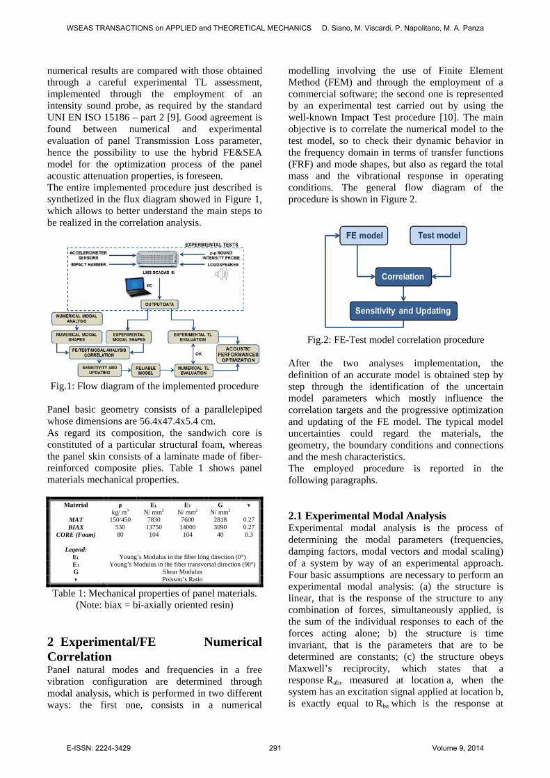
2 Experimental/FE Numerical Correlation Panel natural modes and frequencies in a free vibration configuration are determined through modal analysis, which is performed in two different ways: the first one, consists in a numerical

modelling involving the use of Finite Element Method (FEM) and through the employment of a commercial software; the second one is represented by an experimental test carried out by using the well-known Impact Test procedure [10]. The main objective is to correlate the numerical model to the test model, so to check their dynamic behavior in the frequency domain in terms of transfer functions (FRF) and mode shapes, but also as regard the total mass and the vibrational response in operating conditions. The general flow diagram of the procedure is shown in Figure 2.

Fig.2: FE-Test model correlation procedure

After the two analyses implementation, the definition of an accurate model is obtained step by step through the identification of the uncertain model parameters which mostly influence the correlation targets and the progressive optimization and updating of the FE model. The typical model uncertainties could regard the materials, the geometry, the boundary conditions and connections and the mesh characteristics. The employed procedure is reported in the following paragraphs. 2.1 Experimental Modal Analysis Experimental modal analysis is the process of determining the modal parameters (frequencies, damping factors, modal vectors and modal scaling) of a system by way of an experimental approach. Four basic assumptions are necessary to perform an experimental modal analysis: (a) the structure is linear, that is the response of the structure to any combination of forces, simultaneously applied, is the sum of the individual responses to each of the forces acting alone; b) the structure is time invariant, that is the parameters that are to be determined are constants; (c) the structure obeys Maxwell’s reciprocity, which states that a response Rab, measured at location a, when the system has an excitation signal applied at location b, is exactly equal to Rba which is the response at


E-ISSN: 2224-3429 291 Volume 9, 2014

location b, when that same excitation is applied at a (if Hab is the transfer function between a and be then Hab = Hba); (d) the structure is observable: input/output measurements contain enough information to generate an adequate behavioral model of the structure. The tested panel satisfies all these four assumptions. One of the methodology to acquire modal data is represented by the impact testing. It was developed during the late 1970’s [10], and has become the most popular modal testing method used today. It allows to compute FRF measurements in a FFT (Fast Fourier Transform) analyzer. When the output is fixed and FRFs are measured for multiple inputs, this corresponds to measuring elements from a single row of the FRF matrix. This is typical of a roving hammer impact test, which is the most common type of impact test, and which is also the type of test used in the present work. The necessary equipment to perform the impact test (see Figure 3) is composed by: 1. an impact hammer with a load cell attached to its head to measure the input force; 2. a PCB tri-axial accelerometer to measure the response acceleration at a fixed point (DOF) and directions; 3. a multi-channel FFT analyzer to compute FRFs (Scadas III Acquisition System); 4. a pre and post-processing modal software for identifying modal parameters and displaying the mode shapes in animation (LMS Test.Lab). The module used in this case for the carried out experimental modal analysis is LMS Test.Lab “Impact Testing”. The measurement setup of this software requires as input data: geometry and orientation of the structure, positions of acquisition points (nodes) with respect to the chosen coordinate system, sensitivities of the tri-axial accelerometer (one for each direction) and of the load cell attached to the hammer, frequency range, trigger point. The last-named one is usually set to a small percentage of the peak value of the impulse. The frequency range to excite is fixed so that a Teflon impact hammer head can be used. For testing the panel structure, 81 acquisition points are chosen for the experimental evaluation (Figure 3); these correspond to the DOFs at which the structure is impacted.

Fig.3: Data acquisition through roving hammer

impact test For this purpose the tri-axial accelerometer must be simultaneously sampled together with the force data. The sensitivities are: 0.23 mV/N for the load cell; for the accelerometer 102.5 mV/g in the x direction, 99.7 mV/g in the y direction and 100.8 mV/g in the z direction. The chosen frequency range is fixed up to 3200 Hz. Obviously, it is important to locate the accelerometer in a proper manner, so that its directions coincide with reference ones. FRFs are so computed between each impact DOF and the fixed response DOF. Since accurate impact testing results depend on the skill of one who perform the impact, FRF measurements should be made with spectrum averaging [10]. In the present case each DOF is hit 3 times, therefore each FRF is calculated averaging over 3 instantaneous FRFs. After every impact, it is possible to watch on the screen some plots like those ones shown in Figure 4 which represent the frequency content of the hammer input signal and of the accelerometer response signal, respectively.

Fig.4: From top to bottom: Power Spectrum Density

(PSD) of input force and accelerometer response


E-ISSN: 2224-3429 292 Volume 9, 2014

Note that the plots are referring only to z direction because the input force lies on the negative z axis and thus the z component of response and FRF is the most relevant. In order to obtain sufficiently accurate measurements, it must be paid attention to the shape of the coherence function. If after an impact the coherence function is close to one in the whole considered frequency range, the acquired data can be considered pretty reliable, otherwise the impact has to be repeated. A very well controlled and precise impact excitation needs to be maintained for each of the impacts that constitutes the complete measurement. Figure 5 shows the coherence graph and the averaged FRF amplitude plot of one of the performed measurements.

Fig.5: From top to bottom: averaged FRF amplitude

and coherence After testing, results analysis is carried out. Figure 6 shows the sum of all the averaged z-axis acquired FRFs.

Fig.7: Contribution along z-axis of FRFs sum

In modal analysis, it is possible to use a number of parameter estimation techniques such as LSCE (Least-Squares Complex Exponential) and PolyMax [11]. Estimated poles are calculated and the results of this operation are presented in a so-called stabilization diagram (Figure 7) from which stabilized modes can be picked. Such a diagram

shows the evolution of frequency, damping, and mode/participation vectors as the number of modes is increased.

Fig.7: PolyMax stabilization diagram

To reduce the bias on the modal parameters and to allow the capture of all relevant characteristics of the structure, the identification order is usually chosen quite high. However, the higher the model order is, the higher number of estimated poles will be calculated. But this occurrence could not represent a real physical behavior of the structure. For this reason it is necessary to distinguish physical from mathematical poles. There are several pole-selection methods that allow engineers to pursue this aim. Generally speaking, it is possible to state that physical modes can be seen as those modes for which the frequency, damping, and mode/participation vector values do not change significantly and that they surely have to be searched among FRF peaks [12]. The first ten modal shapes up to 1000 Hz are computed and virtually animated. For sake of brevity only the first three mode shapes experimentally determined are depicted (Figures 8-10). The first one is (1,0) mode that represents the flexural shape in x-direction, the second one is (0,1) mode that is, vice versa, the flexural mode in y-direction, the third one is (1,1) mode representing the flexural mode in both plane directions.

Fig.8: Mode 1 at 288.3 Hz


E-ISSN: 2224-3429 293 Volume 9, 2014



The so calculated experimental mode shapes will be, in the next paragraph, compared with the numerical ones computed in the same frequency range in order to verify the goodness of numerical implementation. 2.2 Numerical Modal Analysis Considering that the panel has a very simple geometry, the CAD model (Figure 11) is directly created in Femap [13] software, used also for the FEM analysis [4].

Fig.11: Panel CAD model

The software Femap (acronym of Finite Element Modeling And Postprocessing) is used in order to build the finite element model of the panel (pre-processing phase). Solution results, obtained with internal MD Nastran solver, are then utilized for FE/Experimental correlation through the employment of LMS Virtual.Lab module. Once created CAD geometry, in the menu Material the

properties of each layup of the panel are set, according to the data reported in Table 1. The sandwich panel is composed of 6 plies as reported in Figure 13. In order to create an accurate mesh model capable to reply the real one, a complicated sandwich model has been set. More precisely, the core is modeled as an isotropic material (foam) while the skin is modeled as a 2D orthotropic material (matrix + reinforcement) [14]. In Layup menu, after establishing panel stratification of 6 plies (Figure 12), the composite equivalent properties are calculated.

Fig. 12: Panel plies

The successive step consists in setting in the Property menu the option Laminate and in adding the value of the nonstructural mass relative to the resin presence. The menu Mesh is then used to establish the maximum number of elements to reach the numerical results in the investigated frequency range (0-1000 Hz). The panel is divided in 81 (9x9) QUAD elements, delimited by 100 (10x10) nodes (see Figure 13).

Fig.13: Panel shell model


E-ISSN: 2224-3429 294 Volume 9, 2014

It is important to underline that in order to perform a numerical modal analysis is useless to define a load set because normal modes are inherent properties of a structure and they depend only on the material properties and on the structure applied constraints. In this case the panel is modelled according to a “free-free” configuration, in the same conditions in which experimental analysis, has been performed. The output results will be imported in the Virtual.Lab environment to define the FE correlation analysis to be implemented in. Figures 14-16 show the first three of the total ten calculated modal shapes. Also in this case, the first one represents the flexural shape in x-direction, the second one the flexural mode in y-direction and the third one the flexural mode in both plane directions.




2.3 Correlation study Both numerical and experimental results in terms of natural mode shapes and frequencies of the panel, are shown and compared in Table 2.

Mode no. Modal frequency [Hz]

m,n Numerical Experimental

1 286.5 288.3

1,0 0.62 %

2 419.3 393.8

0,1 6.48 %

3 508.2 516.8

1,1 1.66 %

4 579.2 588.2

2,2 1.53 %

5 649.2 665.9

0,2 2.5 %

6 709 758.5

1,2 6.53 %

7 794.9 833.8

2,0 4.67 %

8 829.9 899.7

2,1 7.76 %

Table 2: Comparison between sandwich panel numerical and experimental modal analysis

It is evident that a good agreement is found up to a frequency of 1000 Hz because of the low error percentages (<10%). However, in order to validate the FE model a modal shapes correlation study, has to be performed. The correlation phase is focused on comparing, understanding and evaluating correlation between Test and FE data. The final scope is eventually to modify design parameters improving the correlation and to progressively update the model, also in terms of material properties. The MAC (Modal Assurance Criterion) index represents a possible correlation criterion to be used. MAC index is defined as:

{ } { }( ){ } { }

{ } { }( ){ } { }( )FEt

FEtestt

test

FEt

testFEtestMAC

ΨΨΨΨ

ΨΨ=ΨΨ **

2*

, (2)

where { }testΨ and { }FEΨ are the modal vectors computed respectively in the experimental and numerical analyses, too. MAC allows to quantify the modal shapes correlation (from 0 to 1), pointing out the possible presence of missing modes (not square matrix)


E-ISSN: 2224-3429 295 Volume 9, 2014

and/or switching mode (matrix diagonal inversion), and expressing the orthogonality (0) or the parallelism (1) of two any vectors. Firstly, in order to verify the correlation of the experimentally determined modal shapes, an Auto-MAC analysis [15] is carried out (Figure 17). Obtained results show that the computed modes are not combined between them, because the extra-diagonal values are lower than the critical threshold value of 20%.

Fig.17: MAC - Modal Assurance Criterion of the

experimental modes (Auto-MAC) MAC methodology is used also for Test-FE data correlation. Figure 18 demonstrates that modes correlation is mostly good, in fact only MAC diagonal values are different from zero and greater than 0.7, which is indicative of a good correlation between the two compared models. In particular, MAC lower diagonal values are those highlighted.

Fig.18: MAC for Test-FE correlation

These results allow to validate the defined FE model, without the necessity to implement a successive sensitivity and updating procedure. The accuracy of the FE model allows to implement a further numerical 3D analysis to point out the acoustic performances of the system under investigation. 3 Panel Acoustic Performances Evaluation The most important acoustic quantity is the sound pressure, which is an acoustic first-order quantity [16]. However, sources of sound emit sound power, and sound fields are also energy fields in which potential and kinetic energies are generated, transmitted and dissipated. In spite of the fact that the radiated sound power is a negligible part of the energy conversion of almost any sound source, energy considerations are of enormous practical importance in acoustics. Sound intensity is a measure of the flow of acoustic energy in a sound field. More precisely, the sound intensity I is a vector quantity defined as the time average of the net flow of sound energy through a unit area in a direction perpendicular to the area. The dimensions of the sound intensity are energy per unit time per unit area (W/m2). The advent of sound intensity measurement systems in the1980s has had a significant influence on noise control engineering. Sound intensity measurements make it possible to determine the sound power of sources without the use of costly special facilities such as anechoic and reverberation rooms. In some cases the environmental conditions must be kept in account to investigate the coupled source-environment behavior; in other cases the measure must be done in situ on big scale objects. In both these applications the sound intensity method represents an attractive alternative to the conventional techniques. Specifically, sound intensity analysis allows to determine typical material acoustic properties such as the surface impedance and the absorption coefficients, the Noise Reduction, the Insertion Loss and the Transmission Loss parameters [17]. Among these, Transmission Loss (TL) is a key quantification of the effectiveness of acoustical treatments for engineering applications [18]. TL parameter can be considered the quantity of sound (expressed in decibels) absorbed by the structure at a given frequency. Usually, it is measured in 1/3 frequency octave band intervals. It


E-ISSN: 2224-3429 296 Volume 9, 2014

is possible to affirm that structures having same geometry but different material show different ability in transmit sound in air and so different TL values. Analytically, the Transmission Loss of an acoustical material is defined as the ratio of sound intensity incident on the material (Wi) to the amount of sound energy that is transmitted through the same material (Wt). TL coefficient expressed in decibels (dB) is defined as:

t

i

WW

TL 10log10= (1)

The standard test methods for the Transmission Loss measurement uses two adjacent rooms with an adjoining transmission path [19]. The treatment under test is placed between the two rooms in the adjoining transmission path. Sound is generated in one room and measurements are taken in both the source and receiver room to characterize the Transmission Loss. The standard method avoids the direct measurement of the sound energy transmitted in the material by using a reverberation room. This method is defined, time tested, and reliable. Unfortunately, implementing this testing method reliably requires large and expensive test chambers. In many situations where the Transmission Loss tests are necessary but infrequent, this cost and space burden is unacceptable. A Transmission Loss testing procedure that is less costly and requires less space would be of great interest in this situation. The first alternative technique utilizes sound intensity to experimentally determine the Transmission Loss. This method has been standardized by the American Society of Testing and Materials (ASTM) in the standard ASTM E22492 [20]. A broadband sound source is placed in the reverberation, or source, room. The material under test is secured using an open window between the rooms. The sound intensity incident on the material is calculated from the space averaged sound pressure in the source room, under the assumption that the sound field is diffuse. The sound intensity transmitted through the material is then measured in the anechoic chamber, or receiver room, using a sound intensity probe. The intensity probe is positioned perpendicular to the test sample and can be scanned or moved point by point over the material surface to obtain the averaged transmitted sound intensity. A photograph of the set-up is shown in Figure 19. Disadvantage of the set-up is its size and related to this the cost of the measurement.

Fig.19: Standard set-up to measure the Transmission

Loss of acoustic material Under some conditions, it is also possible to measure the Transmission Loss in a standing wave tube [18]. In this case a sample of test material is necessarily needed. 3.1 Experimental Transmission Loss Assessment To determine the Transmission Loss of the panel, sound intensity method has been implemented carrying out experiments through the use of the pressure-pressure (p-p) sound intensity probe (Figure 20). The p-p measurement principle employs two closely spaced pressure microphones [21]. As known, sound intensity is the time-averaged product of the pressure and particle velocity. The particle velocity component in the direction of the axis of the probe is obtained by a finite-difference approximation to the pressure gradient in Euler’s equation of motion. The sound pressure is simply the average of the two pressure signals.

Fig.20: Pressure-pressure sound intensity probe

Taking in account that the smaller the spacer between the two microphones, the higher the frequency that can be measured, the chosen spacer length has been 12 mm so to measure up to 5000 Hz. Figure 21 shows the panel meshing points at which the measurements have been made (81 points).


E-ISSN: 2224-3429 297 Volume 9, 2014

Fig.21: Photograph of the panel in acoustically

treated laboratory The experimental setup (Figure 22) consists in a loudspeaker which provides an acoustic excitation (white noise) to the surface of the panel, the probe that measures the transmitted sound intensity at each of the defined points, and LMS SCADAS III acquisition system that, in addition to acquiring measurements data, sends a reference signal to the loudspeaker. According to the standard UNI EN ISO 15186 - part 2 [9], the incident contribution of sound intensity is determined. Therefore, the TL factor at each of the investigate points is computed from the ratio of the acoustic power associated with the incident and the transmitted waves.

Fig.22: Flux diagram of experimental TL testing

3.2 3D Numerical Transmission Loss Assessment When investigating acoustical problems, mainly discretization methods such as Finite Element Method or Boundary Element Methods, are applied. Both methodologies are well suited for those problems, where the physical behavior of an acoustic medium , such as air, can be described by

Helmholtz equation. The coupled BEM/FEM method is applicable to solution of sound transmission or radiation problems (Seybert, et al., 1985). However, too much computation time is consumed by using this approach. For this reason, a hybrid approach by using the Finite Element Method (FEM) and the Statistical Energy Analysis (SEA) is used to predict the Sound Transmission Loss up to 2000 Hz. AutoSEA is an interactive vibro-acoustics simulation tool based on the SEA method. In order to calculate the Sound Transmission Loss and the radiation efficiency of the panel under study, a hybrid model must be created in AutoSEA, as shown in the Figure 23. For the hybrid FE&SEA model, TL is the Transmission Loss between an SEA Diffused Acoustic Field (DAF) and an SEA semi-infinite fluid (SIF) separated by a FE subsystem. First the model is built and meshed into the software VA One [22]. The panel under investigation presents the same material properties as described in paragraph 1. To create a sandwich panel in AutoSEA, the material properties of the face sheets and the core are required, separately. The face sheets of the sandwich panel must only be isotropic while the core can be orthotropic. The material properties assumed for the face sheets and the core are listed in Figure 13 and Table 1. The numerical model can be divided in two different analysis: a FEM analysis describing the structural behavior of the panel and a SEA model to implement the experimental evaluation. The FEM model implemented in SEA analysis consists of a total 1833 elements. The normal mode analysis is performed with the external “Nastran” solver for the determination of the natural frequency. The calculated natural frequencies up to 2000 Hz, are close to those calculated in the paragraph 2.2. Next the FE faces are created on the existing mesh. The diffuse acoustic field (DAF) is applied on these FE faces. A semi infinite fluid, which is a baffled acoustic half space describing the radiation of sound into an unbounded space, is connected to the panel as shown in Figure 23. Finally, a complete hybrid model is built.


E-ISSN: 2224-3429 298 Volume 9, 2014

Fig. 23: Sound transmission model FE&SEA hybrid method

The TL is calculated by determining the net power radiated into the SEA semi-infinite fluid, and then normalizing the net power by the incident power associated with the DAF (Diffuse Acoustic Field). The results depend on both the pressure difference between the DAF and SEA semi-infinite fluid and the FE faces area A. The loss factor of the panel shell is 1% and no special noise treatment is applied on it. The calculated Transmission Loss parameter derived by the coupled SEA and FEM analysis has been then compared with the experimental one and showed in Figure 18, in the next paragraph. 3.3 Experimental/Numerical Transmission Loss Comparison Obtained results coming from experimental and numerical Transmission Loss evaluation are showed and compared in Figure 24, which reports the experimental and the numerical overall TL level of the panel as functions of the frequencies expressed in one-third octave bands. It is apparent that, over the whole considered frequency range, the computed results with the above mentioned numerical approach match very well with the measured ones. A good accordance can be noted between the two trends, as the maximum deviation is about 4 dB. These results allow to definitely validate the defined FE model, also for determining material acoustic performances. Having now available a panel reliable numerical model, further developments could regard the possibility to implement a Reverse Engineering procedure [23], in order to realize an optimization process by considering different materials or different panel thicknesses, so to improve the acoustic attenuation properties.

0 400 800 1200 1600 2000Frequency (Hz)

8

12

16

20

24

28

32

Tran

smis

sion

Los

s (d

B)

TL Experimental (dB)TL Numerical (dB)

Experimental and Numerical Transmission Loss Comparison

Fig.24: Experimental/Numerical TL comparison

4 Conclusion In the present work a deep study of the acoustic performances of a composite sandwich panel, used for a high speed train, has been realized through the implementation of both experimental and numerical analyses. The panel model used for vibro-acoustic was successfully developed and validated, both structurally and modally through the employment of experimental investigations. The vibro-acoustic model was also successfully developed and validated for TL parameter in a frequency range 0-2000 Hz, again with the experimental results. More precisely, a preliminary experimental and numerical modal analyses correlation procedure has been carried out finding a good agreement between them. The good correlation between test and FE models has then allowed to employ the FE model to numerically assess the Transmission Loss (TL) parameter of the sandwich panel through a hybrid FE&SEA simulation. The numerical TL parameter has been finally compared with panel experimentally determined Transmission Loss property. As results are in good match, future developments could regard the acoustic optimization of the sandwich panel. Taking in account the presence of a less performing acoustic behavior of the system under study at the lower frequencies, these latter certainly represent the frequency range at which an acoustic performances improvement will be desirable.

DAF FE mesh

FE Faces


E-ISSN: 2224-3429 299 Volume 9, 2014

References [1] http://www.sandwichpanels.org. [2] R. M. Christensen, Fiber Reinforced Composite

Materials, Applied Mechanics Reviews, Volume 38, Issue 10, pp. 1267-1270, 1985, doi:10.1115/1.3143688.

[3] QUARTIERI J.; TROISI A; GUARNACCIA C; LENZA TLL; DAGOSTINO P; DAMBROSIO S; IANNONE G., An Acoustical Study of High Speed Train Transits. WSEAS TRANSACTIONS ON SYSTEMS. Volume 8, Issue 4, pp. 481-490 ISSN:1109-2777, 2009.

[4] Siano D., Three-dimensional/one-dimensional numerical correlation study of a three pass perfored tube, Simulation Modelling Practice and Theory, Volume 19, Issue 4, April 2011, pp. 1143-1153, ISSN 1596-190X, 10.1016/j.simpat.2010.04.005.

[5] Siano D., Auriemma F., Bozza F. (2010), Pros and Cons of Using Different Numerical Techniques for Transmission Loss Evaluation of a Small Engine Muffler, In : Small Engine Technology Conference (SETC) 2010, Lintz (Austria), DOI: 10.4271/2010-32-0028.

[6] Siano D., Esposito Corcione F., FE fluid-structure interaction/experimental transmission loss factor comparison of an exhaust system, SAE TECHNICAL PAPER (2005), ISSN: 0148-7191.

[7] Siano D., Amoroso F. , FEM/BEM numerical modeling of a diesel engine acoustic emission, In: 19th International Congress on Acoustics - ICA 2007, International Commission for Acoustics, ISBN: 84-87985-12-2, Madrid.

[8] Li, Z., Vibration and acoustical properties of sandwich composite materials, PhD Thesis, Auburn University (2006).

[9] Acoustics - Measurement of sound insulation in buildings and of building elements using sound intensity - Part 2: Field measurements (ISO 15186-2:2003).

[10] B. J. Schwarz and M.H. Richardson, Experimental Modal Analysis, CSI Reliability Week, Orlando, FL, USA, 1999.

[11] LMS Test.Lab Solutions Guide Manual. [12] J. Lanslots, B. Rodiers, B. Peeters,

Automated pole-selection: proof-of-concept & validation, In Proceedings of ISMA 2004, The International Conference on Noise and Vibration Engineering, Leuven, Belgium, 20-22 September 2004.

[13] Femap Guide Manual. [14] A. Lakshminarayana, R. Vijaya Kumar, G.

Krishna Mohana Rao, Buckling Analysis of Quasi-Isotropic Symmetrically Laminated

Rectangular Composite Plates with an Elliptical/circular Cutout Subjected to Linearly Varying In-Plane Loading Using Fem, INTERNATIONAL JOURNAL of MECHANICS, Issue 1, Volume 6, 2012.

[15] LMS Virtual.Lab Solutions Guide Manual. [16] Jacobsen F., Sound intensity and its

measurement and applications, Acoustic Technology, Technical University of Denmark, Lyngby, Denmark, 2011, Note Number 31262.

[17] D'Ortona V., Vivolo M., Pluymers B., Vandepitte D., & Desmet W. (2013). Experimental identification of noise reduction properties of honeycomb panels using a small cabin, Transport Research Arena 2014, Paris.

[18] A. R. Barnard and M. D. Rao, Measurement of Sound Transmission Loss Using a Modified Four Microphone Impedance Tube, Noise-Con 04, Baltimore (July 2004).

[19] J.C.S. Lai, M. Burgess, Application of the Sound Intensity Technique to Measurement of Field Sound Transmission Loss, Applied Acoustics, Volume 34, Issue 2, 1991, pp. 77–87.

[20] Standard Test Method for Laboratory Measurement of Airborne Transmission Loss of Building Partitions and Elements Using Sound Intensity, American Standard ASTM E 2249 – 02: 2003 (American Society of Testing and Materials 2003).

[21] Daniel Fernandez Comesana, Jelmer Wind, Andrea Grosso, Keith Holland, Performance of p-p and p-u intensity probes using Scan & Paint, 18th International Congress on Sound & Vibration ICSV18, Rio De Janeiro, Brazil, July 2011.

[22] ESI-group: Va one 2007 user guide (2007). [23] T. Suresh Babu, Romy D. Thumbanga,

Reverse Engineering, CAD\CAM & Pattern Less Process Applications in Casting - A Case Study, INTERNATIONAL JOURNAL of MECHANICS, Issue 1, volume 5, 2011.


E-ISSN: 2224-3429 300 Volume 9, 2014

http://www.sandwichpanels.org/

http://appliedmechanicsreviews.asmedigitalcollection.asme.org/solr/searchresults.aspx?author=R.+M.+Christensen&q=R.+M.+Christensen

http://www.naun.org/main/NAUN/mechanics/20-092.pdf



numerical and experimental acoustic performance investigations of · pdf file ·...

Documents