numerical analysis - virginia tech€¦ · 1 notes for numerical analysis math 5465 b y s. adjerid...
TRANSCRIPT

1
Notes for Numerical Analysis
Math 5465
by
S. Adjerid
Virginia Polytechnic Institute
and State University
(A Rough Draft)

2

Contents
1 Solving Eigenvalue Problems 5
1.1 Basic facts about eigenvalues . . . . . . . . . . . . . . . . . . . 51.2 Power methods . . . . . . . . . . . . . . . . . . . . . . . . . . 11
1.2.1 The basic power method . . . . . . . . . . . . . . . . . 111.2.2 The Inverse power method . . . . . . . . . . . . . . . . 151.2.3 The power method for symmetric matrices . . . . . . . 16
1.3 Rayleigh quotient iteration . . . . . . . . . . . . . . . . . . . . 181.4 The QR algorithm . . . . . . . . . . . . . . . . . . . . . . . . 18
1.4.1 Householder and Givens transformations . . . . . . . . 181.4.2 Application of Householder transformations . . . . . . 211.4.3 Review of Schur factorization and more . . . . . . . . . 241.4.4 The basic QR algorithm . . . . . . . . . . . . . . . . . 271.4.5 The QR factorization . . . . . . . . . . . . . . . . . . . 281.4.6 Convergence of the QR algorithm . . . . . . . . . . . . 311.4.7 The QR algorithm with shifts . . . . . . . . . . . . . . 331.4.8 Simultaneous iterations . . . . . . . . . . . . . . . . . . 36
3

4 CONTENTS

Chapter 1
Solving Eigenvalue Problems
1.1 Basic facts about eigenvalues
Matrix eigenvalue problems have many important applications in science andengineering such as
� Stability of di�erential equations
� Data compression and image processing
� Internet search engines, e.g., Google
� Finding roots of polynomials
Example:
y0(t) = Ay(t); y(0) = y0
where
A = P�1�P; � = diag(�1; �2)
Thus the solution is
y(t) = P�1�e�1t 00 e�2t
�Py0:
5

6 CHAPTER 1. SOLVING EIGENVALUE PROBLEMS
De�nition 1. An eigenvalue of an n�n matrix A is the scalar value � suchthat det(A� �I) = 0. The associated eigenvector is a vector v 6= 0 such thatAv = �v.
De�nition 2. The matrices A and B are similar if there exists an invertiblematrix P such that A = PBP�1.
De�nition 3. The characteristic polynomial of a matrix A is p(�) = det(A��I).
Remarks:
� A n�nmatrix A has n eigenvalues counting multiple roots and allowingcomplex roots.
� For each eigenvalue � there exists an eigenvector v 6= 0
Example:
A =
241 2 10 1 32 1 1
35
det(A� �I) = det
241� � 2 1
0 1� � 32 1 1� �
35
= p(�) = ��3 + 3�2 + 2�+ 8 = �(�� 4)(�2 + �+ 2)
The eigenvalues of A are
� = 4; � =�1� i
p7
2
The eigenvector associated with � = 4 is a solution to the system
�3x1 + 2x2 + x1 = 0 (1.1)
0x1 � 3x2 + 3x3 = 0 (1.2)
2x1 + x2 � 3x3 = 0 (1.3)
1.1. BASIC FACTS ABOUT EIGENVALUES 7
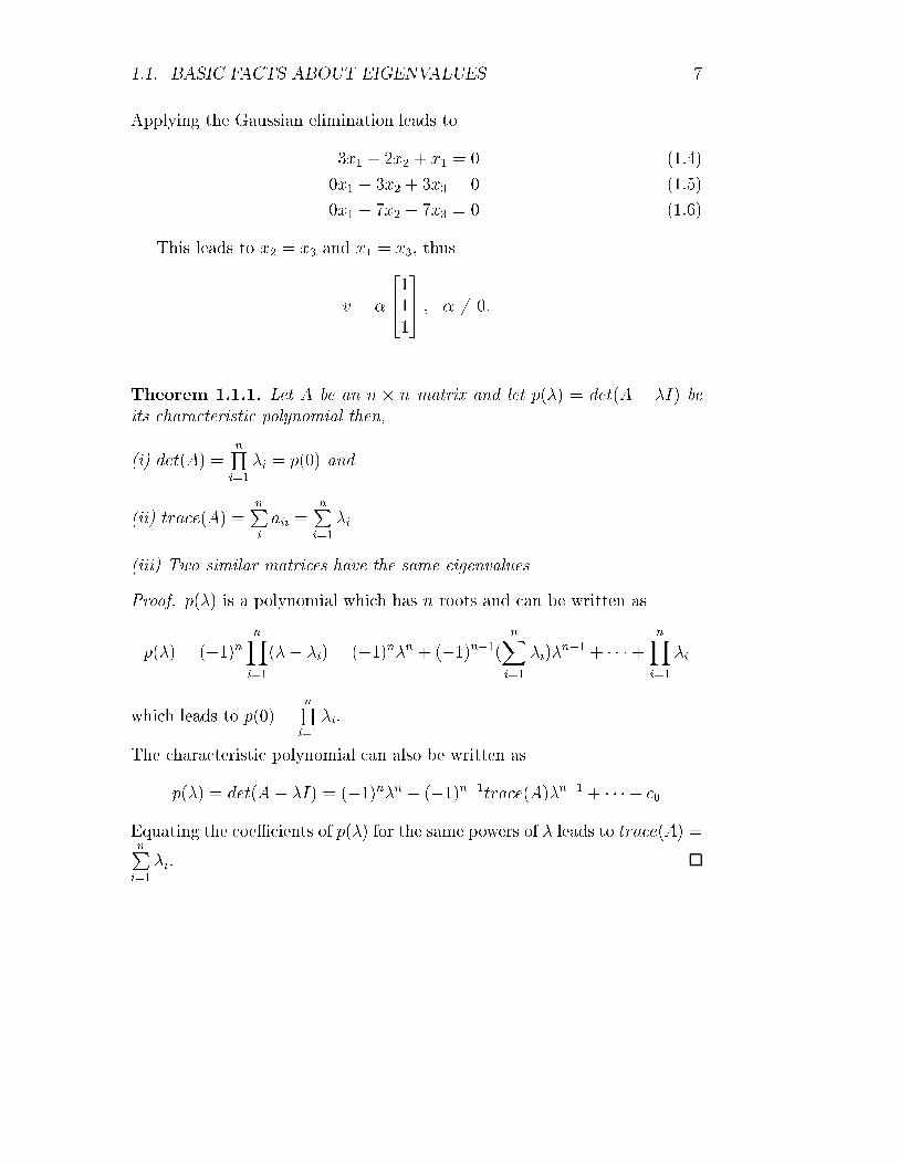
Applying the Gaussian elimination leads to
�3x1 + 2x2 + x1 = 0 (1.4)
0x1 � 3x2 + 3x3 = 0 (1.5)
0x1 + 7x2 � 7x3 = 0 (1.6)
This leads to x2 = x3 and x1 = x3, thus
v = �
24111
35 ; � 6= 0:
Theorem 1.1.1. Let A be an n � n matrix and let p(�) = det(A � �I) beits characteristic polynomial then,
(i) det(A) =nQi=1
�i = p(0) and
(ii) trace(A) =nPi
aii =nPi=1
�i
(iii) Two similar matrices have the same eigenvalues
Proof. p(�) is a polynomial which has n roots and can be written as
p(�) = (�1)nnYi=1
(�� �i) = (�1)n�n + (�1)n�1(nXi=1
�i)�n�1 + � � �+
nYi=1
�i
which leads to p(0) =nQi=1
�i.
The characteristic polynomial can also be written as
p(�) = det(A� �I) = (�1)n�n + (�1)n�1trace(A)�n�1 + � � �+ c0
Equating the coeÆcients of p(�) for the same powers of � leads to trace(A) =nPi=1
�i.

8 CHAPTER 1. SOLVING EIGENVALUE PROBLEMS
Theorem 1.1.2. If A has n distinct eigenvalues �1; � � � ; �n, the associatedeigenvectors v1; v2; � � � ; vn are linearly independent.
De�nition 4. A set of vectors v1; v2; � � � ; vn is orthogonal if vi � vj = Æij
De�nition 5. A matrix P is said to be orthogonal is it column vectors areorthogonal, i.e., P t = P�1 or P tP = PP t = I,
Theorem 1.1.3. If A is a symmetric n� n matrix then,
� All eigenvalues of A are real
� The associated eigenvectors form an orthogonal basis, i.e., they arelinearly independent
Theorem 1.1.4. If A is symmetric positive de�nite then all eigenvalues liein the positive real axis, i.e., �i > 0; i = 1; � � � ; n.Proof. Consult the book on Linear Algebra by Johnson, Riess and Arnold.
Theorem 1.1.5. (Gershgorin theorem): If A is an n � n matrix let Di be
the disk centered at aii with radius ri =nP
j=1;j 6=ijaijj then
� All eigenvalues of A are contained in [ni=1Di
� If union of k disks does not intersect the remaining n � k disks, thenit contains exactly k eigenvalues.
Proof. From Av � �v = 0 and let i such that jvij = jjvjj1. The ith equationyields
aiivi +nX
j=1;j 6=iaijvj = �vi
(aii � �)vi = �nX
j=1;j 6=iaijvj
1.1. BASIC FACTS ABOUT EIGENVALUES 9
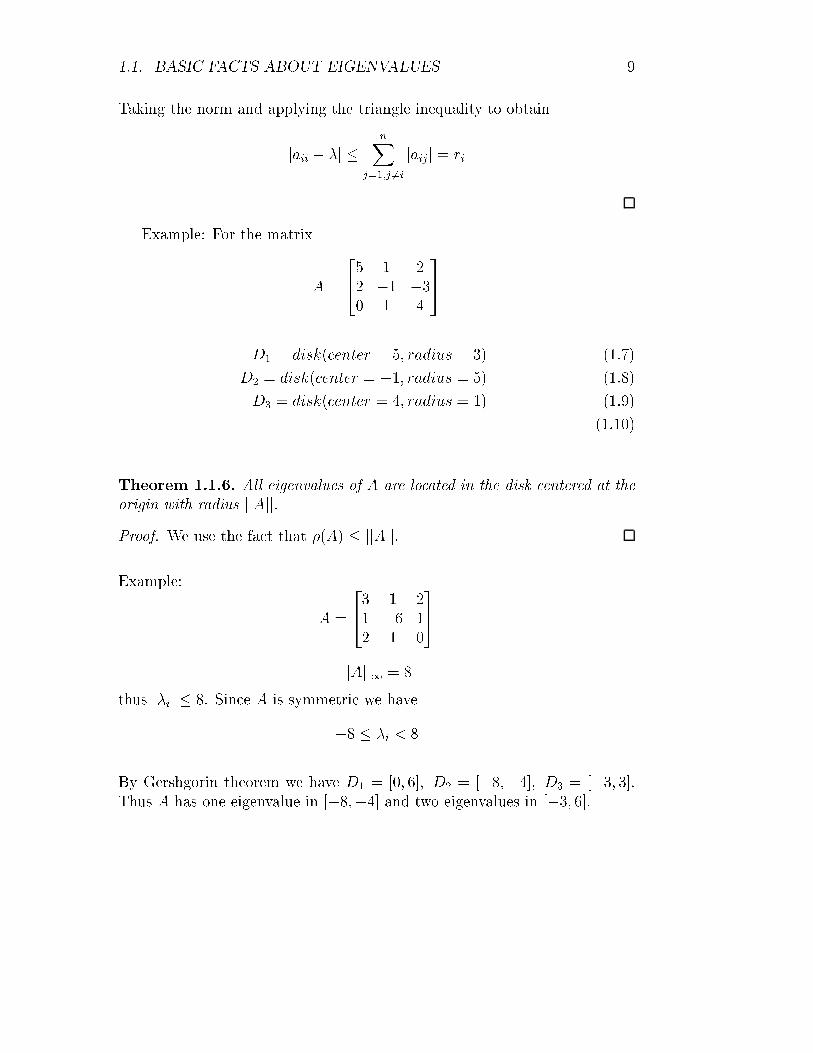
Taking the norm and applying the triangle inequality to obtain
jaii � �j �nX
j=1;j 6=ijaijj = ri
Example: For the matrix
A =
245 1 22 �1 �30 1 4
35
D1 = disk(center = 5; radius = 3) (1.7)
D2 = disk(center = �1; radius = 5) (1.8)
D3 = disk(center = 4; radius = 1) (1.9)
(1.10)
Theorem 1.1.6. All eigenvalues of A are located in the disk centered at theorigin with radius jjAjj.Proof. We use the fact that �(A) � jjAjj.
Example:
A =
243 1 21 �6 12 1 0
35
jjAjj1 = 8
thus j�ij � 8. Since A is symmetric we have
�8 � �i < 8
By Gershgorin theorem we have D1 = [0; 6]; D2 = [�8;�4]; D3 = [�3; 3].Thus A has one eigenvalue in [�8;�4] and two eigenvalues in [�3; 6].
10 CHAPTER 1. SOLVING EIGENVALUE PROBLEMS
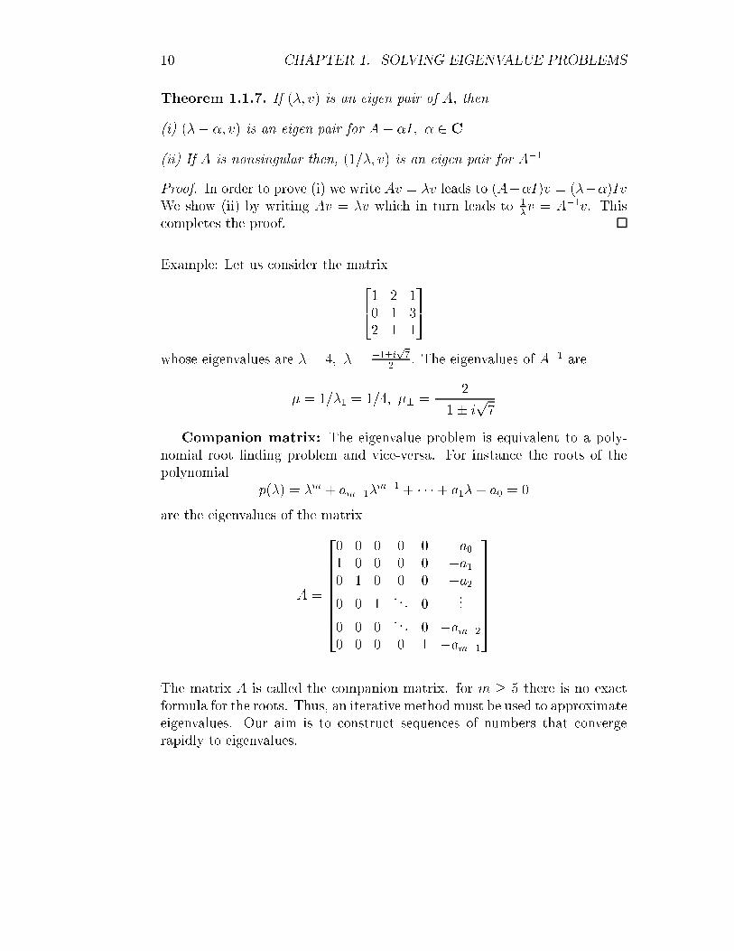
Theorem 1.1.7. If (�; v) is an eigen pair of A, then
(i) (�� �; v) is an eigen pair for A� �I; � 2 C
(ii) If A is nonsingular then, (1=�; v) is an eigen pair for A�1
Proof. In order to prove (i) we write Av = �v leads to (A��I)v = (���)IvWe show (ii) by writing Av = �v which in turn leads to 1
�v = A�1v. This
completes the proof.
Example: Let us consider the matrix241 2 10 1 32 1 1
35
whose eigenvalues are � = 4; � = �1�ip72
. The eigenvalues of A�1 are
� = 1=�1 = 1=4; �� =2
�1� ip7
Companion matrix: The eigenvalue problem is equivalent to a poly-nomial root �nding problem and vice-versa. For instance the roots of thepolynomial
p(�) = �m + am�1�m�1 + � � �+ a1� + a0 = 0
are the eigenvalues of the matrix
A =
266666664
0 0 0 0 0 �a01 0 0 0 0 �a10 1 0 0 0 �a20 0 1
. . . 0...
0 0 0. . . 0 �am�2
0 0 0 0 1 �am�1
377777775
The matrix A is called the companion matrix. for m � 5 there is no exactformula for the roots. Thus, an iterative method must be used to approximateeigenvalues. Our aim is to construct sequences of numbers that convergerapidly to eigenvalues.

1.2. POWER METHODS 11
1.2 Power methods
1.2.1 The basic power method
Before we state the basic power algorithm we prove the following theorem:
Theorem 1.2.1. Let A be an n�n matrix with eigenvalues �i; i = 1; � � � ; nsuch that
(i) �1; �2; � � � ; �n are the eigenvalues of A such that j�1j > j�2j � j�3j � � � �j�nj
(ii) There exist n linearly independent eigenvectors vi; i = 1; � � � ; n withAvi = �ivi.
(iii) If the vector x0 is such that x0 =nPi=1
�ivi, and �1 6= 0,
Then
limk!1
Akx(0)
�k1= �1v1
and
limk!1
< x(0); Akx(0) >
< x(0); Ak�1x(0) >= �1
Proof. We start from
x(0) = �1v1 + �2v2 + � � �+ �nvn; �1 6= 0
Using the de�nition of eigen pairs we write
Avi = �ivi; Akvi = �ki vi

12 CHAPTER 1. SOLVING EIGENVALUE PROBLEMS
Now we construct the following sequence of vectors
x(1) = Ax(0) (1.11)
x(2) = A2x(0) (1.12)...
... (1.13)
x(k) = Akx(0) (1.14)...
... (1.15)
We note that
x(k) = Ak(�1v1 + �2v2 + � � �+ �nvn) = �1Akv1 + �2A
kv2 + � � �+ �nAkvn
�1�k1v1 + �2�
k2v2 + � � �+ �n�
knvn
= �k1(�1v1 + �2(�2�1)kv2 + � � �+ �n(
�n�1
)kvn
Since j�ij=j�1j < 1; i � 2 we have
x(k)
�k1= �1v1 +O((�2=�1)
k); as k !1 (1.16)
x(k+1)
�k+11
= �1v1 +O((�2=�1)k+1); (1.17)
This shows the �rst part of the theorem.
In order to show the second part we write if �i = (x0)tvi
< x(0); Akx(0) >
< x(0); Ak�1x(0) >=
�1�1 + � � �+ �n�n
�k�11 �1 + � � �+ �k�1n �n
= �1�1 +O(�2=�1)
k)
�1 +O(�2=�1)k�1)
Letting k !1 completes the proof of the theorem.

1.2. POWER METHODS 13
Algorithm for a power method
Step i: select x(0) 6= 0, k = 1, set Nmax; tol; �(0) = 0 and
Step ii: y(k) = Axk�1, �(k) = y(k)p where jy(k)p j = jjy(k)jj1
Step iii: if j�(k) � �(k�1)j < tol or k � NmaxStopelseset x(k) = y(k)=�(k)
Step iv : Go to step ii
Theorem 1.2.2. Under the assumptions of the previous theorem and �(k)
and x(k) as de�ned in the power method we have
(i)limk!1
�(k) = �1
j�(k) � �1j = O((�2�1)k)
Furthermore,
limk!1
x(k) =v1
jjv1jj1and
jjx(k) � akv1jj = O((�2�1)k)
Proof. First, use induction to show that x(k) = ckAkx(0), where ck = 1=
kQi=1
�(k)
x(k) = ck�k1(�1v1 +
nXi=2
�i(�i=�1)kvi) (1.18)
Since by construction the left-hand side leads to jjx(k)jj1 = 1, the right-handside must give
limk!1
ck�k1 =
1
�1jjv1jj1

14 CHAPTER 1. SOLVING EIGENVALUE PROBLEMS
Thus, we conclude that
limk!1
x(k) =v1
jjv1jj1Now we can show that
x(k) � akv1 = ck�k1(
nXi=2
�i(�i=�1)kvi
Since ck�k ! 1
�1jjv1jj1 , we complete the proof of the second part of theorem.
Using (1.18) and
Ax(k�1) = ck�1�k1(�1v1 +
nXi=2
�i(�i=�1)kvi)
�(k) can be written
�(k) = y(k)p = (Ax(k�1))p =(Ay(k�1))p
y(k�1)p
Noting it is the same p since as k !1 y(k) � �1v1=jjv1jj1.Using
y(k�1) = Ax(k�2) = ck�1Ak�1x(0) = ck�1
nXi=1
(�i)k�ivi
We obtain
�(k) = �1
�1v1;p +nPi=2
�i(�i=�1)kvi;p
�1v1;p +nPi=2
�i(�i=�1)k�1vi;p
We note that for k ! 1 the index p such jx(k)p j = jjx(k)jj1 will also corre-spond to the largest component in v1, i.e., jv1;pj = jjv1jj1.
= �11 +O((�2=�1)
k)
1 +O((�2=�1)k)= �1[1 +O((�2=�1)
k�1)]
Thusj�(k) � �1j = O((�2=�1)
k):

1.2. POWER METHODS 15
Remark: we can also prove �(k) ! �1 by noting that
x(k) = y(k)=y(k)p = Ax(k�1)=�(k)
to write�(k)x(k) = Ax(k�1)
Taking the dot product with x(k) and solving for �(k) we obtain
�(k) =(x(k))tAx(k�1)
(x(k))tx(k)! vt1Av1
vt1v1= �1
De�nition 6. The Rayleigh quotient of a vector x 2 Rn is the scalar
r(x) =< x;Ax >
< x; x >
We note that if x is an eigenvector associated with the eigenvalue �, thenr(x) = �
1.2.2 The Inverse power method
For � not an eigenvalue of A, we consider the matrix (A��I)�1 with eigen-values �i =
1�i�� , where �i are the eigenvalues of A. The largest eigenvalue
in magnitude of (A� �I)�1 is �k corresponding to �k the closest eigenvalueto � and thus the power method applied to (A� �I)�1 converges to �k andthus yields �k = � + 1=�k.
By selecting � close to an eigenvalue of interest we will be able to use theinverse power method to compute approximations to non dominant eigenval-ues.
Inverse Power method Algorithm:
step 1: select a � and a vector x(0) such that jjx(0)jj2 = 1, �(0) = 0
for k = 1; 2; � � �
16 CHAPTER 1. SOLVING EIGENVALUE PROBLEMS
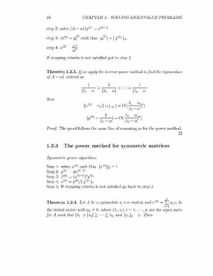
step 2: solve (A� �I)y(k) = x(k�1)
step 3: m(k) = y(k)p such that jy(k)p j = jjy(k)jj1
step 4: x(k) = y(k)
y(k)p
if stopping criteria is not satis�ed got to step 2
Theorem 1.2.3. If we apply the inverse power method to �nd the eigenvaluesof A� �I ordered as
1
j�1 � �j >1
j�2 � �j > � � � > 1
j�n � �jthen
jjz(k) � v1=jjv1jj1jj = O([�1 � �
�2 � �]k)
j�(k) � 1
�1 � �j = O([
�1 � �
�2 � �]k)
Proof. The proof follows the same line of reasoning as for the power method.
1.2.3 The power method for symmetric matrices
Symmetric power algorithm:
Step 1: select x(0) such that jjx(0)jj2 = 1Step 2: y(k) = Ax(k�1)
Step 3: �(k) = (x(k�1))ty(k)
Step 4: x(k) = y(k)=jjy(k)jj2Step 5: If stopping criteria is not satis�ed go back to step 2
Theorem 1.2.4. Let A be a symmetric n � n matrix and x(0) =nPi=1
�ivi be
the initial vector with �1 6= 0, where (�i; vi); i = 1; � � � ; n are the eigen pairsfor A such that j�1j > j�2j � � � � � �n and jjvijj2 = 1. Then

1.2. POWER METHODS 17
limk!1
x(k) = v1=jjv1jj2; jjx(k) � akv1jj2jj2 = O(�2=�1)k)
andj�(k) � �1j = O((�2=�1)
2k)
Proof. In order to prove the convergence of the eigenvector we will use
x(k) = ckAkx(0) = ck�
k1(�1v1 +
nXi=2
�i(�i�1)kvi) (1.19)
Noting that when k!1
x(k) � �k1ck�1v1
we conclude that
limk!1
ck�k1�1 =
1
jjv1jj2This proves the convergence of the eigenvector with ak = ck�
k1�1.
For the eigenvalues since x(k) ! v1=jjv1jj2 the Rayleigh quotient leads to
�(k) = < x(k�1); y(k) > = < x(k�1); Ax(k�1) > = r(x(k�1); A)
Thus, as k !1 �(k) ! �1.We �nish the proof using the fact that the eigenvectors are orthogonal to
write
�(k) =< x(k�1); Ax(k�1) >< x(k�1); x(k�1) >
Using (1.19) we obtain
�(k) = �1
< (�1v1 +nPi=2
�i(�i�1)k�1vi); (�1v1 +
nPi=2
�i(�i�1)kvi) >
< (�1v1 +nPi=2
�i(�i�1)k�1vi); (�1v1 +
nPi=2
�i(�i�1)k�1vi) >
Applying the orthogonality condition < vi; vj >= Æij we have
�(k) = �1
�21 +
nPi=2
�2i (
�i�1)2k�1
�21 +
nPi=2
�2i (
�i�1)2k�2

18 CHAPTER 1. SOLVING EIGENVALUE PROBLEMS
Thus we have established quadratic convergence:
j�(k) � �1j = O(�2=�)2k):
1.3 Rayleigh quotient iteration
Given A an n� n symmetric matrix
Algorithm for Rayleigh quotient iteration
Step 1: select an initial vector x(0) such that jjx(0)jj2 = 1Step 2: compute �(k) = x(k�1)Ax(k�1)
Step 3: solve (A� �(k)I)y(k) = x(k�1)
Step 4 : compute x(k) = y(k)=jjy(k)jj2Step 5 : k = k + 1 go back to step 2.
� The main disadvantage is that at every iteration we update the matrixand thus have to compute a new factorization.
� If A is symmetric we may avoid this problem by using the Householdertransformation and apply the Rayleigh iteration to a tridiagonal matrixwhich makes the factorization step much cheaper with an O(n) oating-point operations.
� We obtain cubic convergence.
1.4 The QR algorithm
We start by introducing the QR method for symmetric matrices using House-holder and Givens transformations.
1.4.1 Householder and Givens transformations
De�nition 7. Householder transformation is de�ned by the matrix
H = I � 2uut
< u; u >

1.4. THE QR ALGORITHM 19
where u 6= 0 2 Rn
Theorem 1.4.1. H is a symmetric and orthogonal matrix
Proof. It is easy to verify that H t = H. Now, let us show that H2 = I
(I � 2uut
< u; u >) (I � 2
uut
< u; u >) = I � 4
uut
< u; u >+ 4
uutuut
< u; u >2= I
We used the fact that uutuut = (utu)uut = < u; u > uut.
Householder transformations may be used to
� zero columns and/or rows
� transform general matrices to Hessenberg matrices
� transform symmetric matrices to similar tridiagonal matrices
� compute QR factorization of matrices
De�nition 8. Givens rotation G(i; j; �) is an orthogonal matrix di�erentfrom the identity at four entries (i; i); (j; j); (i; j) and (j; i)
i j
2666666666666666664
1 0 � � � � � � � � � 0 � � � � � � 0
0. . . 0 � � � ... � � � ...
......
. . . 1 0 � � � � � � 0...
0 � � � 0 c 0 � � � s 0 � � � ......
0 � � � 0 �s 0 � � � c 0 � � � ...... 1 0
...... 0
. . ....
0 � � � � � � � � � � � � � � � � � � � � � 0 1
3777777777777777775
i...j
where c = cos(�) and s = sin(�) for some �.

20 CHAPTER 1. SOLVING EIGENVALUE PROBLEMS
If we consider the vector X = [x1; x2; � � �xn], thenG(i; j; �)X = [x1; � � � ; xi�1; yi; xi+1; � � � ; xj�1; yj; xj+1; � � � ; xn]
where yi = cxi + sxj and yj = �sxi + cxj
In order to make for instance yj = 0 we have
c =xiq
x2i + x2j
; s =xjq
x2i + x2j
One can guard against over ow by using the algorithm
if xj = 0c = 1; s = 0 elseif jxjj > jxij� = �xi=xj, s = 1=
p1 + � 2, c = s�
else� = �xj=xi, c = 1=
p1 + � 2, s = c�
endend
Remarks:
� Givens rotations are orthogonal, i.e., GGt = GtG = I
� Premultiplication by G(i; j; �) amounts to a rotation of � radians in thecounterclockwise direction of the (i; j); j > i coordinates.
� Givens rotations are preferred for selectively zeroing entries of matrices.It will zero one entry at a time.
� Givens rotations may be used to reduce a matrix A into a Hessenbergmatrix with 4n3=3 +O(n2) multiplications.
� Givens rotations may be used to reduce a symmetric matrix into asymmetric tridiagonal matrix
� No need to compute �
� Requires 5 ops and a single square root for each matrix-vector multi-plication
1.4. THE QR ALGORITHM 21
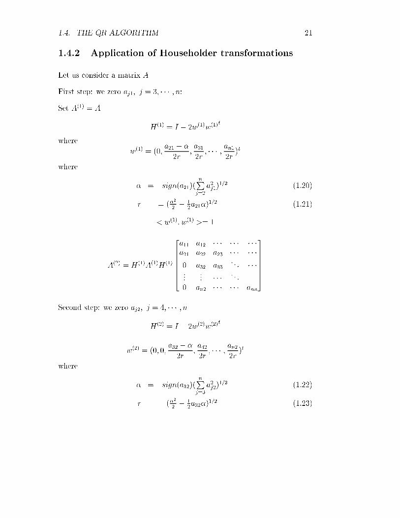
1.4.2 Application of Householder transformations
Let us consider a matrix A
First step: we zero aj1; j = 3; � � � ; n:Set A(1) = A
H(1) = I � 2w(1)w(1)t
where
w(1) = (0;a21 � �
2r;a312r
; � � � ; an12r
)t
where
� = �sign(a21)(nP
j=2
a2j1)1=2 (1.20)
r = (�2
2� 1
2a21�)
1=2 (1.21)
< w(1); w(1) >= 1
A(2) = H(1)A(1)H(1)
2666664
a11 a12 � � � � � � � � �a21 a22 a23 � � � � � �0 a32 a33
. . . � � �...
... � � � . . .
0 an2 � � � � � � ann
3777775
Second step: we zero aj2; j = 4; � � � ; n
H(2) = I � 2w(2)w(2)t
w(2) = (0; 0;a32 � �
2r;a422r
; � � � ; an22r
)t
where
� = �sign(a32)(nP
j=3
a2j2)1=2 (1.22)
r = (�2
2� 1
2a32�)
1=2 (1.23)

22 CHAPTER 1. SOLVING EIGENVALUE PROBLEMS
< w(2); w(2) >= 1
Kth step: we zero ajk; j = k + 2; � � � ; n
A(k) =
2666666666664
a11 a12 � � � � � � � � � ...
a21 a22 � � � � � � � � � ...0 0 � � � akk � � � akn
0 0 � � � ak+1;k � � � ...
0 0 � � � ak+2;k � � � ...
0 0 � � � ... � � � ...0 0 � � � ank � � � ann
3777777777775
H(k) = I � 2w(k)w(k)t
w(k) = (0; � � � ; 0; ak+1;k � �
2r;ak+2;k2r
; � � � ; ank2r
)t
where
� = �sign(ak+1;k)(nP
j=k+1
a2jk)1=2 (1.24)
r = (�2
2� 1
2ak+1;k�)
1=2 (1.25)
< w(k); w(k) >= 1
where sign(0) = 1. After n� 2 steps we obtain
A(k+1) = H(k)A(k)H(k)
leads to
A(n�1) = H(n�2) � � �H(1)AH(1) � � �H(n�2) = HAH t
where
H = H(n�2) � � �H(1)
with A(n�2) being a symmetric tridiagonal matrix similar to A.
A numerical example for a symmetric matrix:

1.4. THE QR ALGORITHM 23
A =
26644 1 �2 21 2 0 1�2 0 3 �22 1 �2 �1
3775
First step of Householder transformation:
q =4X
j=2
a2j1 = 9; � = �1� 3:
2r2 = �2 � �a21 = 12; r =p6
w(1) =1
2r(0; a21 � �; a31; a41)
t =1
2p6(0; 0; 4;�2; 2)t:
H(1) = I � 2w(1)w(1)t =
26641 0 0 00 �1=3 2=3 �2=30 2=3 2=3 1=30 �2=3 1=3 2=3
3775
A(2) = H(1)AH(1) =
26644 �3 0 0�3 10=3 1 4=30 1 5=3 �4=30 4=3 �4=3 1
3775
Second step of Householder transformation:
q = a232 + a242 = 1 +4
3
2
=25
9; � = �sign(1)pq = �5=3
r = (1
2(�2 � �a32))
2 =p5=3
w(2) =1
2r(0; 0; 8=3; 4=3)t; H(2) = I � 2w(2)w(2)t =
26641 0 0 00 1 0 00 0 �3=5 �4=50 0 �4=5 3=5
3775
A(3) = H(2)A(2)H(2) =
26644 �3 0 0�3 10=3 �5=3 00 �5=3 �33=25 68=750 0 68=75 149=75
3775

24 CHAPTER 1. SOLVING EIGENVALUE PROBLEMS
Thus, A(3) is symmetric tridiagonal and similar to A.
In order to apply the kth step of householder transformations for symmetricmatrices we use the following algorithm:
A(k+1) = H(k)A(k)H(k)
= (I � 2w(k)w(k)t)A(k)(I � 2w(k)w(k)t)
= A(k) � 2w(k)w(k)tA(k) � 2A(k)w(k)w(k)t + 4w(k)w(k)tA(k)w(k)w(k)t
= A(k) � 2(w(k)ut + uw(k)t)
whereu = � � aw(k); � = A(k)w(k); a = w(k)t� (1.26)
For symmetric matrices, each Householder step requires 2(n�k)2+O(n)multiplications. The total number of multiplication to transform a symmetricmatrix A into a tridiagonal symmetric matrix is
n�2Xk=1
k2 =n3
3+O(n2)
1.4.3 Review of Schur factorization and more
Decoupling: Some eigenvalue algorithms consist of breaking the problems
into smaller subproblems as stated in the following Theorem.
Lemma 1.4.1. Let A 2 Cn�n be such that
A =
�A11 A12
0 A22
�; :
Then �(A) = �(A11) [ �(A22).
Proof. Let (�; v) be an eignepair of A such that�A11 A12
0 A22
� �v1v2
�= �
�v1v2
�:
If v2 6= 0, then A22v2 = �v2, thus � 2 �(A22). If v2 = 0, then A11v1 = �v1,thus, thus � 2 �(A11). since both sets have same cardinal we have equalityof the two sets.

1.4. THE QR ALGORITHM 25
De�nition 9. We de�ne the range and rank of matrix A as
ran(A) = span(a1:; � � � ; an:); rank(A) = dim(ran(A)):
Lemma 1.4.2. Let A 2 Cn�n, B 2 Cp�p and X 2 Cn�p such that
AX = XB; with rank(X) = p:
Then there exists an orthogonal matrix Q 2 Cn�n such that
QHAQ ==
�T11 T120 T22
�; :
where �(T11) = �(A) \ �(B).
Proof. Let X = Q
�R1
0
�, Q 2 Cn�n, R1 2 Cn�n be the QR factorization of
X.Using the assumption of the lemma and rearraging we write
AQ
�R1
0
�= Q
�R1
0
�B
which yields
QHAQ
�R1
0
�=
�T11 T12T21 T22
� �R1
0
�=
�R1
0
�B:
Since R1 is nonsingular and T21R1 = 0, thus, T21 = 0. T11R1 = R1B , thusT11 and B are similar. By the previous lemma we show that �(A) = �(T ) =�(T11) [ �(T22).
De�nition 10. A matrix Q 2 Cn�n is unitary if and only if QHQ = QQH =I. (this is the equivalent to orthogonal matrices for real matrices)
Now we are ready to establish Schur decomposition in C.
Theorem 1.4.2. Let A 2 Cn�n. There exits a unitary matrix Q 2 Cn�n
such that
QHAQ = D +N; D = diag(�1; � � � ; �n); Nij = 0; i � j:
Furthermore Q can be chosen to the eigenvalues in any order.

26 CHAPTER 1. SOLVING EIGENVALUE PROBLEMS
Proof. The theorem hold for n = 1. Assume it holds for all matrices of ordern � 1 or less. If Ax = �x, where x 6= 0, by the previous lemma, B = [�],there exists a unitary matrix U such that
UHAUH =
�� wH
0 C
�
By induction for C 2 C(n�1)�(n�1) there exits a unitary matrix such as ~UHC ~Uis upper triangular. Thus if Q = Udiag(1; ~U), then
QHAQ = diag(1; ~UH)UHAUdiag(1; ~U) = diag(1; ~UH)
�� wH
0 C
�diag(1; ~U)
QHAQ =
�� wH
0 ~UHC ~U
�
which is upper triangular.
Corollary 1. If A 2 Cn�n is normal, i.e., AHA = AAH , then there exists aunitary matrix Q 2 Cn�n such that
QHAQ = diag(�1; � � � ; �n):
Proof. The Schur decomposition QHAQ = R yields that R is also normal.Finally we note that a normal upper triangular matrix is diagonal.
Real Schur decomposition: The Real Schur decomposition amountsto factoring a real matrix in Rn�n into an orthogonal matrix Q and an upperquasi-triangular matrix R such that
Theorem 1.4.3. If A 2 Rn�n, then there exists an orthogonal matrix Qsuch that
QtAQ = R =
26664R11 R12 � � � R1m
0 R22 � � � R2m...
.... . .
...0 0 � � � Rmm
37775
where Rii is either a 1� 1 or 2� 2 block with complex conjugate eigenvalues.
Proof. Proof consult Matrix Computations by G. Golub and Van Loan

1.4. THE QR ALGORITHM 27
Remark: All real matrices are orthogonally similar to an upper quasi-triangular matrix.
Using Householder transformations, every symmetric matrix is similar to asymmetric tridiagonal matrix obtained by applying Houselholder transfor-mations (n� 2) times.
Next, let A be a symmetric tridiagonal matrix. we will show that Givensrotations will enable us to factor any tridiagonal matrix into a product of anorthogonal matrix Q and an upper triangular matrix R as A = QR.
1.4.4 The basic QR algorithm
The QR method generates a sequence of similar tridiagonal symmetric ma-trices
A(0) = A; A(1); A(2); � � � ; A(k); � � �de�ned as
A = A(0) = Q(0)R(0)
A(1) = R(0)Q(0) = Q(1)R(1)
A(2) = R(1)Q(1) = Q(2)R(2)
......
A(k�1) = R(k�2)Q(k�2) = Q(k�1)R(k�1)
A(k) = R(k�1)Q(k�1) = Q(k)R(k)
(1.27)
Theorem 1.4.4. If a asymmetric matrix, then (i) the matrices A(k) aresimilar matrices, i.e.,
A(k) = (Q(k�1))tA(k�1)Q(k�1)
. Furthermore, if j�1j > j�2j > � � � > j�nj ,
limk!1
A(k) = diag(�1; � � � ; �n)
Proof. The proof will begiven in the end.
28 CHAPTER 1. SOLVING EIGENVALUE PROBLEMS
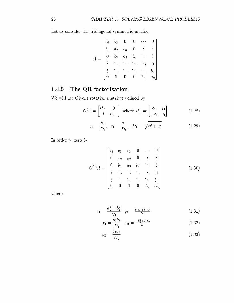
Let us consider the tridiagonal symmetric matrix
A =
26666666664
a1 b2 0 0 � � � 0
b2 a2 b3 0...
...
0 b3 a3 b4. . .
......
. . . . . . . . . . . . 0...
. . . . . . . . . . . . bn0 0 0 0 bn an
37777777775
1.4.5 The QR factorization
We will use Givens rotation matrices de�ned by
G(1) =
�P11 00 In�1
�where P11 =
�c1 s1�s1 c1
�(1.28)
s1 =b2D1
; c1 =a1D1
; D1 =qb22 + a21 (1.29)
In order to zero b2
G(1)A =
26666666664
z1 q1 r1 0 � � � 0
0 x2 y2 0...
...
0 b3 a3 b4. . .
......
. . . . . . . . . . . . 0...
. . . . . . . . . . . . bn0 0 0 0 bn an
37777777775
(1.30)
where
z1 =a21 + b22D1
q1 =b2a1+b2a2
D1(1.31)
r1 =b2b3D1
x2 =�b22+a1a2
D1(1.32)
y2 =b3a1D1
(1.33)

1.4. THE QR ALGORITHM 29
We remark that G1(G(1))t = (G(1))tG(1) = I
At the kth step:
G(k) =
24Ik�1 0 0
0 Pkk 00 0 In�k�1
35 ; Pkk =
�ck+1 sk+1�sk+1 ck+1
�
sk+1 =bk+1Dk
; ck+1 =xkDk; Dk =
qb2k+1 + x2k (1.34)
A(k) =
2666666666666664
z1 q1 r1 0 0 � � � � � � 0
0. . . . . . . . . . . . � � � � � � ...
zk�1 qk�1 rk�1 0 � � � ...
0 � � � 0 xk yk 0 0...
0 bk+1 ak+1 bk+2. . .
...... � � � . . . . . . . . . . . . . . . 0...
. . . . . . . . . . . . . . . . . . bn0 � � � � � � � � � � � � 0 bn an
3777777777777775
In order to zero bk+1 we compute
G(k)A(k) = A(k+1)
where
zk = Dk
xk+1 = �ykbk+1+xkak+1Dk
yk+1 =bk+2xkDk
rk = bk+1bk+2Dk
qk = bk+1(xk+ak+1)Dk
After n� 1 steps we obtain
R = A(n) = G(n�1)G(n�1) � � �G(1)A

30 CHAPTER 1. SOLVING EIGENVALUE PROBLEMS
which can be written as
A = (G(1))t(G(2))t � � � (G(n�1))tR = QR
where R is an upper triangular matrix with rij = 0; j > i + 2 and
Q = (G(1))t(G(2))t � � � (G(n�1))t
is an upper Hessenberg matrix.
Example:
A =
243 1 01 3 10 1 3
35
G(1) =
24 3=
p10 1=
p10 0
�1=p10 3=p10 0
0 0 1
35
G(1)A =
24p10 3
p10=5 1=
p10
0 4p10=5 3=
p10
0 1 3
35
G(2) =
241 0 0
0 4p10=
p185
p185=37
0 �p185=37 4p10=
p185
35
A(3) = G(2)A(2) =
24p10 3
p10=5 1=
p10
0p185=5 27=
p185
0 0 21p185=37
p10
35
Q = (G(1))t(G(2))t =
243=
p10 �4=p185 1=
p74
1=p10 12=
p185 �3=p74
0p185=37 4=
p74
35

1.4. THE QR ALGORITHM 31
A = QR
To transform a symmetric matrix to a tridiagonal symmetric matrix we mayapply Givens rotations (n� 2)(n� 1)=2 times and each step requires 4(n�i) multiplications. To reduce to zero the elements in row (i � 1) we need4(n� i)2 multiplications. Thus, the total number of multiplications requiredto transform a symmetric matrix into a tridiagonal symmetric matrix is
n�1Xk=1
4(n� k)2 =4n3
3+O(n2)
1.4.6 Convergence of the QR algorithm
If we assume that A is an upper Hessenberg with n eigenvalues ordered asj�1j � j�2j � � � � j�nj, Then the pth subdiagonal entry of A(k), a
(k)p+1;p, exhibits
a linear convergence rate to zero:
ja(k)p+1;pj = O(
�����p+1�p
����k
)
Remarks:
� If j�pj = j�p+1j, A(k) the QR may not converge.
� If �n is much closer to zero than all other eigenvalues, the (n; n � 1)entry of A(k) converges to zero rapidly.
� If a(k)j+1;j = O(Eps), where Eps is the machine precision, then the matrix
can be split into two smaller problems A(k)1 and A
(k)2 , where
A =
�A1 00 A2
�

32 CHAPTER 1. SOLVING EIGENVALUE PROBLEMS
� If j�1j > j�2j > � � � > j�nj and �i 2 R; then
A(k) !
26664�1 � � �0 �2 � �...
.... . . �
0 � � � 0 �n
37775
Examples where the symmetric QR algorithm fails to converge to a diag-onal matrix.Example 1:
A =
�0 11 0
�where Q = A and R = I.
A =
240 0 10 1 01 0 0
35
Hessenberg form of A is
A(0) =
241 0 00 0 �10 �1 0
35
In general whenever a matrix has two eigenvalues such that �1 = ��2, theQR algorithm fails to converge to a diagonal matrix.
Next, we give nonsymmetric example what the QR algorithm fails to con-verge.Example: Let us consider the companion matrix of p5(x) = x5 + 1 given as
A =
2666640 0 0 0 �11 0 0 0 00 1 0 0 00 0 1 0 00 0 0 1 0
377775
whose eigenvalues are on the unit circle ,i.e., j�ij = 1Applying the QR algorithm we �nd that A = A(1) = Q(1)R(1) where
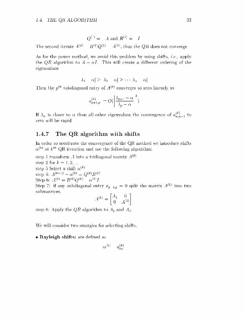
1.4. THE QR ALGORITHM 33
Q(1) = �A and R(1) = �IThe second iterate A(2) = R(1)Q(1) = A(1), thus the QR does not converge.
As for the power method, we avoid this problem by using shifts, i:e:, applythe QR algorithm to A � �I. This will create a di�erent ordering of theeigenvalues
j�1 � �j � j�2 � �j � � � � j�n � �jThen the pth subdiagonal entry of A(k) converges to zero linearly as
ja(k)p+1;pj = O(
�����p+1 � �
�p � �
����k
)
If �n is closer to � than all other eigenvalues the convergence of a(k)n;n�1 to
zero will be rapid.
1.4.7 The QR algorithm with shifts
In order to accelerate the convergence of the QR method we introduce shifts�(k) at kth QR iteration and use the following algorithm:
step 1 transform A into a tridiagonal matrix A(0)
step 2 for k = 1; 2; :::step 5 Select a shift �(k)
step 4: A(k�1) � �(k) = Q(k)R(k)
Step 6: A(k) = R(k)Q(k) + �(k)IStep 7: if any subdiagonal entry ap+1;p = 0 split the matrix A(k) into twosubmatrices.
A(k) =
�A1 00 A(2)
�step 8: Apply the QR algorithm to A1 and A2.
We will consider two stratgies for selecting shifts.
� Rayleigh shifts: are de�ned as
�(k) = a(k)nn

34 CHAPTER 1. SOLVING EIGENVALUE PROBLEMS
The QR algorithm with Rayleigh shifts converges quadratically for genericmatrices but fails to converge, for instance, for the matrix
A =
�0 11 0
�
� Wilkinson shifts: which consists of(i) �nding the eigenvalues �1 and �2 of the 2� 2 matrix�
an�1 bnbn an
�
(ii) Select �(0) = �1 the closest eigenvalue to an .
In general, for k > 1 we have �(k) = �1 the closest eigenvalue of
"a(k)n�1 b
(k)n
b(k)n a(k)n
#
to a(1)n and is given as
�(k) = a(k)n � sign(Æ)(b
(k)n )2
jÆj+qÆ2 + (b
(k)n )2
;
where
Æ = (a(k)n�1 � a(k)n )=2; sign(Æ) =
(1 ifÆ � 0
�1 otherwise
If b(k)n = 0, then
� � = a(k)n is an eigenvalue
� Apply the QR algorithm for the (n� 1)� (n� 1) matrix
A =
266666664
a(k)1 b
(k)2 0 � � � 0
bk2. . . . . . . . .
...
0. . . . . . . . . 0
.... . . . . . . . . b
(k)n�1
0 � � � 0 b(k)n�1 a
(k)n�1
377777775
Remarks:

1.4. THE QR ALGORITHM 35
� Cubic convergence for the generic case, i.e., a(k)n converges cubically to
an eigenvalue
� Quadratic convergence in the worst case (using exact arithmetic)
For instance, let us consider the matrix for which the QR algorithm fails toconverge:
A =
�0 11 0
�:
The eigenvalues are � = �1 we take a shift �(1) = �1 to get
A+ I =
�1 11 1
�
Q =1
2
��p2 �p2�p2 p
2
�; R =
��p2 �p20 0
�
A(1) = QtRQ =
�2 00 0
�
A(1) =
�2 00 0
�� I =
�1 00 �1
�Thus the shifted QR algorithm converges in one iteration.
Eigenvectors: IfA = H tA(0)H
which leads to AH t = H tA(0). Thus if (�; w) is an eigen pair of A(0), i.e.,A(0)w = �w, this leads to AH t = �H tw. Thus, (�;H tw) is an engen pair ofA.
For the QR algorithmA(k) = ( �Qk)tA(0) �Q(k)
where �Q(k) = Q(1) : : : Q(k)
lim( �Q(k))t = [w1; : : : ; wn]; where jjwijj2 = 1:
Thus the eigenvectors of A are vi = H twi.

36 CHAPTER 1. SOLVING EIGENVALUE PROBLEMS
1.4.8 Simultaneous iterations
Gram-Schmidth orthogonalization
First we begin by reviewing the Gram-Schmidth method starting from a setof linearly independent vectors
V = fv1; v2; v3; : : : ; vmg
to de�ne a set of orthonormal vectors asq1 =
v1jjv1jj2
qk =vk�
k�1P
j=1<vk;qj>qj
jjvk�k�1P
j=1<vk;qj>qj jj2
; k = 2; : : : ; m
Thus,
vk =
kXj=1
< vk; qj > qj; k = 1; 2; : : :
We can write in matrix form:
[v1; v2; : : : ; vm] = [q1; q2; : : : ; qm]
264r11 r12 : : :
0 r22...
......
...
375
where rij =< vj; qi > and rii = jjvj �j�1Pi=1
rijqijj2.
In practice this algorithm is numerically unstable, instead we use a modi�edGram-Schmidth algorithm see page 277 of Cheney and Kincaid.
Simultaneuous iterations
If A is a symmetric n� n matrix such that
j�1j > j�2j > : : : > j�mj > j�m+1j � : : : � j�nj
andQ̂ = [q1; q2; : : : ; qm]; such that Aqi = �iqi

1.4. THE QR ALGORITHM 37
Now, let us consider
V (0) = [v(0)1 ; : : : ; v(0)m ]; vi 2 Rn
an n�m matrix such that all leading principal minors of Q̂tV (0) are nonsin-gular.Next, we apply A to V (0) to obtain
V (k) = AkV (0) = [Akv(0)1 ; : : : ; Akv(0)m ]
Theorem 1.4.5. Let A be a symmetric matrix. If V (k) = Q̂(k)R(k), then
limk!1
Q̂(k) = [�q1;�q2; : : : ;�qm]
such that
jjq(k)j ��qjjj = O(Ck); C = max1�k�m
j�k+1jj�kj
Proof. Using the diagonalization of A with the transformation matrix Q =[q1; : : : ; qn] we write
V (k) = AkV (0) = Q�kQtV (0)
splitting � as
� =
��̂ 00 ��
�we write as k !1
V (k) = Q̂�̂kQ̂tV (0) +O(j�m+1jk)Since by assumption Q̂tV (0) is nonsingular we can write
V (k) = (Q̂�̂k +O(j�m+1jk))Q̂tV (0)
and the column space for V (k) is the same as that for
B = Q̂�̂k +O(j�m+1jk):Since all leading principal minors are nonsingular, the previous result holdfor all subsets of V (0). This leads to the following statements:
1. The �rst column of V (k) is proportional to the �rst column of B

38 CHAPTER 1. SOLVING EIGENVALUE PROBLEMS
2. The �rst and second columns of V (k) span the same space as the �rstand second columns of B
Now using the QR factorization we have
V (k) = Q(k)R(k) =
[r11q(k)1 ; r12q
(k)1 + r22q
(k)2 ; : : : ;
iXj=1
rjiq(k)j ; : : : ; q(k)m ] =
([�k1q1; �k2q2; : : : ; �
kmqm] +O(�m1jk))Q̂tV (0):
Simultaneous iterations
The previous method is numerically unstable. Instead we consider a methodthat applies orthogonalization at every power iteration to obtain algorithm:
Select Q̂(0) 2 Rn�m with orthogonal columnsfor k=1,2, ....Z(k) = AQ̂(k�1) ( de�ne Z(k) )Z(k) = Q̂(k)R̂(k) (factor Z(k) )
One can show that the column spaces of Z(k) and Q̂(k) are the same: �rst let
Z(1) = AQ̂(0)
which is factored as
Z(1) = Q(1)R(1)
Next, we write
Z(2) = AQ(1)
which yields after multiplication by R(1)
Z(2)R(1) = AQ(1)R(1) = AZ(1) = A2Q(0) = V (2):

1.4. THE QR ALGORITHM 39
For arbitrary k we have
Z(k)R(k�1) : : : R(1) = AkQ̂(0) = V (k):
Thus the column space of Z(k) is the same as that of V (k).
Theorem 1.4.6. Under the assumptions of the prevous theorem we have
q(k)j ! �qj; as k !1:
Equivalence between the QR and simultaneous iteration algorithms
Simultaneous Iteration:
Q(0) = I
Z = AQ(k�1)
Z = Q(k)R(k)
de�ne: A(k) = (Q(k))tAQ(k)
Unshifted QR algorithm:
A(0) = AA(k�1) = Q(k)R(k)
A(k) = R(k)Q(k)
de�ne Q(k) = Q(1) : : : Q(k)
For both algorithms we de�ne the m�m matrixde�ne R(k) = R(k) : : : R(1)
Theorem 1.4.7. The two algorithms generate identical matrices R(k), Q(k)
and A(k) withAk = Q(k)R(k):
Furthermore we haveA(k) = (Q(k))tAQ(k)
Proof. The proof is obtained using induction. for k = 0 it is trivial. for bothmethods we obtain A0 = Q(0) = R(0) = I and A(0) = A.
The case k � 1.

40 CHAPTER 1. SOLVING EIGENVALUE PROBLEMS
For the simultaneous iteration we assume
Ak�1 = Q(k�1)R(k�1)
and write
Ak = AAk�1 = AQ(k�1)R(k�1) = ZR(k�1) =
Q(k)R(k)R(k�1) = Q(k)R(k)
we have used the fact Z = AQ(k�1) = Q(k)R(k).
For the QR algorithm we follow the same line of reasoning. First we assumethat
Ak�1 = Q(k�1)R(k�1)
and
A(k�1) = (Q(k�1))tAQ(k�1)
which is equivalent to
Q(k�1)A(k�1) = AQ(k�1)
Now we write
Ak = AAk�1 = AQ(k�1)R(k�1) = Q(k�1)A(k�1)R(k�1) = Q(k)R(k)
In the last step we used
A(k�1) = Q(k)R(k)
In order to establish the second statement of the theorem: (i) In the simul-taneous iteration it is obtained by de�ntion (ii) In the QR algorithm we usethe recursion as
A(k) = (Q(k))tA(k�1)Q(k) = (Q(k))t : : : (Q(1))tAQ(1) : : : Q(k)
In the next theorem we state the convergence of the QR algorithm forsymmetric matrices.

1.4. THE QR ALGORITHM 41
Theorem 1.4.8. Let the basic QR algorithm be applied to a real symmetricmatrix A whose eigenvalues satisfy
j�1j > j�2j > : : : > j�nj
and whose corresponding eigenvectors are given in the matrix Q = [q1; : : : ; qn]whose leading principal minors are nonsingular. Then
limk!1
A(k) = diag(�1; �2; : : : ; �n)
linearly with a constant C = maxk=1::n
j�k+1j=j�kjFurthermore, Q(k) converges linearly (with constant C) to Q with signs
ajusted as necessarily.