numerical analysis of the losses in unsteady flow through...
TRANSCRIPT
Open Journal of Fluid Dynamics 2013 3 252-260 Published Online December 2013 (httpwwwscirporgjournalojfd) httpdxdoiorg104236ojfd201334031
Open Access OJFD
Numerical Analysis of the Losses in Unsteady Flow through Turbine Stage
Sławomir Dykas Włodzimierz Wroacuteblewski Dawid Machalica Institute of Power Engineering and Turbomachinery Silesian University of Technology Gliwice Poland
Email slawomirdykaspolslpl
Received August 12 2013 revised September 12 2013 accepted September 20 2013
Copyright copy 2013 Sławomir Dykas et al This is an open access article distributed under the Creative Commons Attribution License which permits unrestricted use distribution and reproduction in any medium provided the original work is properly cited
ABSTRACT
This paper presents an analysis of the operation of a stage of an aircraft engine gas turbine in terms of generation of flow losses The energy loss coefficient the entropy loss coefficient and an additional pressure loss coefficient were adopted to describe the losses quantitatively Distributions of loss coefficients were presented along the height of the blade channel All coefficients were determined based on the data from the unsteady flow field and analyzed for differ- ent mutual positioning of the stator and rotor blades The flow calculations were performed using the Ansys CFX com- mercial software package The analyses presented in this paper were carried out using the URANS (Unsteady Rey- nolds-Averaged Navier-Stokes) method and two different turbulence models the common Shear Stress Transport (SST) model and the Adaptive-Scale Simulation (SAS) turbulence model which belongs to the group of hybrid models Keywords Turbine Stage Stator Rotor Loss Coefficients
1 Introduction
Aerodynamic losses in the flow through a turbine stage have an adverse impact on energy conversion efficiency Obviously due to the turbine stage specificity the nature of these losses is unsteady This is mainly related to the impact of the rotating rotor blade ring with the stationary stator blade ring and the intense turbulent phenomena which are responsible for blade losses [1] These losses include as follows [2] Profile losses which result from the friction of the
viscous fluid against the blade surface as well as from the finite thickness of the trailing edge behind which the so-called aerodynamic wake is formed
Boundary losses which result from the effect that the near-wall layer and the medium flowing in the blade channel have on each other The medium velocity in the near-wall boundary layer area on the surfaces limiting the channel from top and bottom is lower than in the remaining part of the channel This leads to an imbalance of the forces resulting from the dis- tribution of pressure and the deflection of the medium stream Consequently streamlines get deflected to- wards the base of the blade channel as well as in the direction of the convex (sucking) blade surface The intensity of the described phenomena increases as the
blade channel relative height becomes smaller Losses resulting from incomplete feed These losses
occur in some steam turbines fed with high-parameter steam and in small gas turbines They result from the fact that the stages used in such structures are not fed at full perimeter Losses related to incomplete feed manifest themselves by gas being pushed out of the rotor channels which due to the rotation of the rotor found themselves before the fed nozzle segment and by the gas being mixed in areas at the edge of the feeding segment
Losses related to the cooling of the first stages of the gas turbine
The energy dissipation phenomena occurring in a tur- bine stage are more and more often analyzed by means of the computational fluid dynamics (CFD) tools [3-5] This paper presents the methodology and the results of CFD analyses comprising the unsteady flow in the turbine stage of an aircraft engine [6] The use of the Ansys CFX commercial software package makes it possible to iden-tify places where losses arise and in many cases allows their physical interpretation The energy loss coefficient the entropy loss coefficient and an additional pressure loss coefficient [12] were adopted to describe the losses quantitatively The analyses presented in this paper were
S DYKAS ET AL
Open Access OJFD
253
carried out using the URANS method and two different turbulence models the common Shear Stress Transport (SST) model and the Adaptive-Scale Simulation (SAS) turbulence model which belongs to the group of hybrid models The aim of the comparison of results obtained from analyses conducted with different turbulence mod- els was to show whether the application of the SAS model which is much more demanding in terms of equipment is justified in the type of simulation under discussion
2 Definitions of Loss Coefficients and Their Physical Interpretation
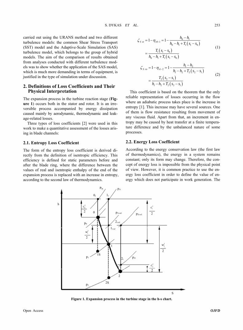
The expansion process in the turbine reaction stage (Fig- ure 1) occurs both in the stator and rotor It is an irre- versible process accompanied by energy dissipation caused mainly by aerodynamic thermodynamic and leak- age-related losses
Three types of loss coefficients [2] were used in this work to make a quantitative assessment of the losses aris- ing in blade channels
21 Entropy Loss Coefficient
The form of the entropy loss coefficient is derived di- rectly from the definition of isentropic efficiency This efficiency is defined for static parameters before and after the blade ring where the difference between the values of real and isentropic enthalpy of the end of the expansion process is replaced with an increase in entropy according to the second law of thermodynamics
0 1 0 1
0 1 1 1 0
1 1 0
0 1 1 1 0
1 1 S st s
h h
h h T s s
T s s
h h T s s
(1)
1 2 1 2
1 2 2 2 1
2 2 1
1 2 2 2 1
1 1S ro s
h h
h h T s s
T s s
h h T s s
(2)
This coefficient is based on the theorem that the only reliable representation of losses occurring in the flow where an adiabatic process takes place is the increase in entropy [1] This increase may have several sources One of them is flow resistance resulting from movement of any viscous fluid Apart from that an increment in en- tropy may be caused by heat transfer at a finite tempera- ture difference and by the unbalanced nature of some processes
22 Energy Loss Coefficient
According to the energy conservation law (the first law of thermodynamics) the energy in a system remains constant only its form may change Therefore the con- cept of energy loss is impossible from the physical point of view However it is common practice to use the en- ergy loss coefficient in order to define the value of en- ergy which does not participate in work generation The
1
1S
2
2S
S
h
0
0t 1t
p1tP0t
p1t rel p2t rel
2t rel
1t rel
p1
p0
2tp2t
p2
2
2
2
2
2c
2
2w
2
1w
2
2
1c2
0c
2
Figure 1 Expansion process in the turbine stage in the h-s chart
S DYKAS ET AL
Open Access OJFD
254
form of this coefficient was derived from the energy conservation law which statesmdashfor the stator blade ring mdashthat total enthalpy is constant while constant rothalpy is assumed for the rotor blade ring For perfect gas it may eventually be written using total and static pressures
1
1
11 1 1
0 11
0
1
1 1
1
ttEn st
t s
t
p
ph hideal gas
h hp
p
(3)
1
2
2 2 2 1
1 22
1
1
1 1
1
t relt relEn ro
t rel s
t rel
p
ph hideal gas
h hp
p
(4)
23 Pressure Loss Coefficient
This is one of the most common loss coefficients in use Its popularity results from the fact that determination of the parameters needed to find the coefficient is very easy This feature is essential in experimental testing where static and total pressure measurements are commonly applied and relatively easy to perform
0 1
0 1
t tP st
t
p p
p p
(5)
1 2
1 2
t rel t relP ro
t rel
p p
p p
(6)
The pressure loss coefficient relates a loss of total pressure in the blade ring to the theoretical value of dy- namic pressure that the medium would feature at the ro- tor outlet if loss pt did not occur This loss may be caused
by friction presence of shock waves etc
3 Turbine Stage Geometry
This work presents an analysis of the unsteady flow in a gas turbine intended for the aircraft industry and de- scribed in [6] The characteristic feature of the turbine is that it has just one stage which distinguishes it from other turbines used in turbofan engines Another impor- tant factor in the selection of the turbine stage was the publication of complete geometry of the blades and op- erating parameters of the analyzed stage in [6] The stage under consideration is composed of 36 381 mm high stator blades located at an average radius of 4699 mm and 64 rotor blades with the same height and radius of location Due to the lack of data concerning the geometry of the tip seal of the rotor blades a geometry was se- lected that is typical for this stage type The geometry of the stage under analysis is presented in Figure 2
An unstructured hybrid-type mesh composed of ap- proximately 550 k nodes for each blade channel was used to discretize the computational domain One channel for the stator blade ring and two channels for the rotor blade ring were assumed for the computations This gives 17 M mesh nodes in total The mesh of the tip seal of the rotor blades was generated as fully structured It is com- posed of approximately 300 k nodes While making the mesh special care was taken to achieve accurate discre- tization in the near-wall boundary layers ensuring y+ asymp 1
The boundary conditions used in the analysis are pre- sented in Table 1 The very high drop in pressure be- tween the stage inlet and outlet makes the flow field much more complex Two turbulence modelsmdashthe Shear Stress Transport (SST) and the Scale-Adaptive Simula- tion (SAS) [7] were used in the performed numerical simulations
hub mean tip
Figure 2 Geometry of the analyzed turbine stage
S DYKAS ET AL
Open Access OJFD
255
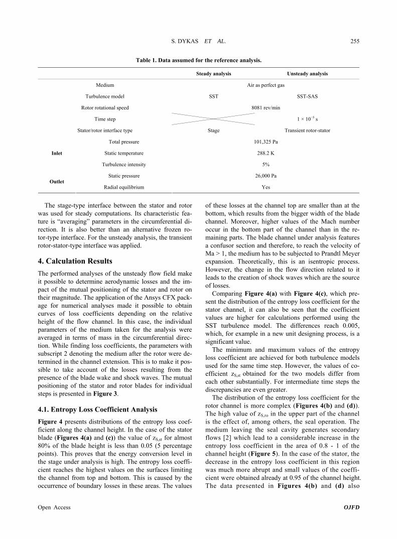
Table 1 Data assumed for the reference analysis
Steady analysis Unsteady analysis
Medium Air as perfect gas
Turbulence model SST SST-SAS
Rotor rotational speed 8081 revmin
Time step 1 times 10minus5 s
Statorrotor interface type Stage Transient rotor-stator
Total pressure 101325 Pa
Static temperature 2882 K Inlet
Turbulence intensity 5
Static pressure 26000 Pa Outlet
Radial equilibrium Yes
The stage-type interface between the stator and rotor
was used for steady computations Its characteristic fea- ture is ldquoaveragingrdquo parameters in the circumferential di- rection It is also better than an alternative frozen ro- tor-type interface For the unsteady analysis the transient rotor-stator-type interface was applied
4 Calculation Results
The performed analyses of the unsteady flow field make it possible to determine aerodynamic losses and the im- pact of the mutual positioning of the stator and rotor on their magnitude The application of the Ansys CFX pack- age for numerical analyses made it possible to obtain curves of loss coefficients depending on the relative height of the flow channel In this case the individual parameters of the medium taken for the analysis were averaged in terms of mass in the circumferential direc- tion While finding loss coefficients the parameters with subscript 2 denoting the medium after the rotor were de- termined in the channel extension This is to make it pos- sible to take account of the losses resulting from the presence of the blade wake and shock waves The mutual positioning of the stator and rotor blades for individual steps is presented in Figure 3
41 Entropy Loss Coefficient Analysis
Figure 4 presents distributions of the entropy loss coef-ficient along the channel height In the case of the stator blade (Figures 4(a) and (c)) the value of zSst for almost 80 of the blade height is less than 005 (5 percentage points) This proves that the energy conversion level in the stage under analysis is high The entropy loss coeffi- cient reaches the highest values on the surfaces limiting the channel from top and bottom This is caused by the occurrence of boundary losses in these areas The values
of these losses at the channel top are smaller than at the bottom which results from the bigger width of the blade channel Moreover higher values of the Mach number occur in the bottom part of the channel than in the re- maining parts The blade channel under analysis features a confusor section and therefore to reach the velocity of Ma gt 1 the medium has to be subjected to Prandtl Meyer expansion Theoretically this is an isentropic process However the change in the flow direction related to it leads to the creation of shock waves which are the source of losses
Comparing Figure 4(a) with Figure 4(c) which pre- sent the distribution of the entropy loss coefficient for the stator channel it can also be seen that the coefficient values are higher for calculations performed using the SST turbulence model The differences reach 0005 which for example in a new unit designing process is a significant value
The minimum and maximum values of the entropy loss coefficient are achieved for both turbulence models used for the same time step However the values of co- efficient zSst obtained for the two models differ from each other substantially For intermediate time steps the discrepancies are even greater
The distribution of the entropy loss coefficient for the rotor channel is more complex (Figures 4(b) and (d)) The high value of zSro in the upper part of the channel is the effect of among others the seal operation The medium leaving the seal cavity generates secondary flows [2] which lead to a considerable increase in the entropy loss coefficient in the area of 08 - 1 of the channel height (Figure 5) In the case of the stator the decrease in the entropy loss coefficient in this region was much more abrupt and small values of the coeffi-cient were obtained already at 095 of the channel height The data presented in Figures 4(b) and (d) also
S DYKAS ET AL
Open Access OJFD
256
453525 15 1
Figure 3 Mutual positioning of the statorrotor blades for individual time steps
0
02
04
06
08
1
0 005 01
rela
tiv
e s
pa
n
152535451
1
08
06
04
02
0 0 005 01
45
35
25
15
1
Rel
ativ
e sp
an
ζSst
0
02
04
06
08
1
0 01 02 03
rela
tive
span
S ro
15
25
35
45
1
ζSro (a) (b)
0
02
04
06
08
1
0 005 01
rela
tiv
e sp
an
S st
152535451
1
08
06
04
02
0
0 005 01
ζSst
45
35
25
15
1
Rel
ativ
e sp
an
0
02
04
06
08
1
0 01 02 03
relative span
S ro
15
25
35
45
1
1
08
06
04
02
0
0 01
ζSro
45
35
25
15
1
Rel
ativ
e sp
an
02 03
(c) (d)
Figure 4 Distribution of the entropy loss coefficient for reference analyses (low temperatures) (a) stator SST (b) rotor SST (c) stator SAS (d) rotor SAS indicate that the entropy loss coefficient for almost the entire height of the channel assumes values higher than 01 This proves that the efficiency of the analyzed rotor blade ring is much lower than that of the stator
At 03 of the relative height of the channel coefficient zSro reaches values bigger than 015 This is related to the substantial increment in the entropy of the medium in the trailing edge area At this height the increment is clearly bigger than in the remaining part of the channel (Figure 6) Also in the area of ~03 of the relative height of the
channel the biggest changes in the loss coefficient occur depending on the mutual statorrotor positioning These changes probably result from the unsteady nature of the blade wake vortices and from the shock waves arising in the trailing edge region
In the case of the rotor blade ring channel a big dis- crepancy is observed between the entropy loss coefficient values calculated for the results obtained using different turbulence models The difference is especially notice- able in the area of 02 - 03 of the relative height of the
S DYKAS ET AL
Open Access OJFD
257
5136e+002
3852e+002
2568e+002
1284e+002
3758e-004[m s-1]
Veiocity Streamine 1
Y
Y
Z
Figure 5 Generation of reverse flows in the area where the medium leaving the seal mixes with the main flow
4000e+002Static Entropy Tmarvg
3000e+002
2000e+002
1000e+002
0000e+002
30 10 70
Relative span
J kg-1K-1
Figure 6 Distribution of static entropy in the rotor channel reference analysis SAS turbulence model
channel where the values assumed by coefficient zSro are high The SAS model located the mentioned area at a bigger height of the channel compared to the SST model Moreover for the SST turbulence model the values of zSro in this area diverge less from the values assumed in other regions of the blade The fluctuations in the values of zSro are in this region higher for the SST model and reach 003
42 Energy Loss Coefficient Analysis
Figures 7(a) and (c) present distributions of the energy loss coefficient along the height of the stator blade The amplitude of fluctuations in the values of zEnst decreases rather uniformly with the blade height Above 097 of the channel relative height the curves formed for individual time steps coincide The biggest changes in the energy
loss coefficient occur at 02 of the channel relative height where they reach 0035
In the case of the SST turbulence model an intersec- tion of zEnst curves occurs for subsequent time steps 25 and 35 This proves that there is a phase shift in changes in the energy loss coefficient for areas above and below the point of intersection As this point is situated in the upper part of the blade where amplitudes of fluctuations in the values of zEnst are slight the phase shift mentioned above will have little effect on ldquosmoothingrdquo the ampli- tudes of changes in the loss coefficient calculated for the entire stator blade ring It is the big amplitude of the changes in the bottom part of the channel that has a deci- sive impact on how the coefficient evolves
Figures 7(b) and (d) show distributions of values of the energy loss coefficient calculated for the channel
S DYKAS ET AL
Open Access OJFD
258
0
01
02
03
04
05
06
07
08
09
1
0 005 01
rela
tive
span
15
25
35
45
1
0
01
02
03
04
05
06
07
08
09
1
0 01 02 03
rela
tive
span
15
25
35
45
1
ζEnst ζEnro
(a) (b)
0
01
02
03
04
05
06
07
08
09
1
0 005 01
rela
tive
span
15
25
35
45
1
0
01
02
03
04
05
06
07
08
09
1
0 01 02 03
rela
tive
span 15
25
35
45
1
ζEnst ζEnro
(c) (d)
Figure 7 Distributions of the energy loss coefficient for reference analyses (low temperatures) (a) stator SST (b) rotor SST (c) stator SAS (d) rotor SAS of the rotor blade ring The biggest difference between the values of zEnro for both turbulence models is visible in the bottom part of the channel At ~01 of the blade relative height it exceeds 003 In this area there is also a difference between the values of fluctuations in zEnro These fluctuations feature slightly bigger amplitudes in the case of results obtained using the SST turbulence model
At 03 of the channel relative height (where previously an especially big increment in the entropy of the medium was observed in the trailing edge region) the SAS turbu- lence model gave a much larger increase in the energy loss coefficient than that modelled by the SST model This may indicate a significant impact of the turbulence phenomena in this region which are better mapped by the SAS model on the energy loss coefficient value
In the figures presenting distributions of the energy loss coefficient values for the rotor channel no intersec- tions of curves are observed for time steps subsequent to each other
In this situation the fluctuations in average values of
zEnro calculated for the entire blade can be seen quite clearly
Moreover it can be noticed that low values of zEnst
correspond to high values of zEnro The changes in values of the energy loss coefficient for individual blade rings will in a way balance each other reducing fluctuations in the average value of the loss coefficient calculated for the entire stage
43 Pressure Loss Coefficient Analysis
Figures 8(a) and (c) present distributions of the pressure loss coefficient for the channel of the stator blade ring Their shape is similar to the shape of zEnst curves because both coefficients are functions of the same parameters of the medium As it was the case for the energy and en- tropy loss coefficients the values of zPst are smaller for the calculation results obtained using the SAS turbulence model The differences between the results of the two models reach 002 (time step ldquo1rdquo and 02 of the channel relative height)
The range of changes in the values of the pressure loss
S DYKAS ET AL
Open Access OJFD
259
coefficient for the stator channel decreases with its height At 02 of the channel relative height fluctuations in the values of zPst amount to as much as 0055 At the same time it can be seen that the changes in values of the pressure loss coefficient along the channel entire length do not run in the same direction This is proved by sev- eral intersections of curves for time steps 15 25 and 35
Figures 8(b) and (d) present distributions of the pres- sure loss coefficient for the rotor blade ring The most significant difference between the values of this coeffi- cient for the SST and SAS turbulence models occurs in the bottom part of the flow channel Here for the SAS model the pressure loss coefficient assumes values smaller even by 007 At the same time fluctuations in the values of zPro for this particular turbulence model (SAS) feature bigger amplitudes The maximum range of the fluctuations is achieved at 01 of the channel relative height where it assumes the value of 011 Fluctuations in zPro in the upper part of the blade are very slight In principle a noticeable amplitude occurs only at the point
of deflection of the curves at 08 of the channel relative height A change in the value of zPro in this region may result from unsteady operation of the seal
Considering the impact of the mutual statorrotor posi- tioning on the zPro value a drop in value of the pressure loss coefficient can be observed for the first three time steps (mutual statorrotor positions) In the next steps the value rises This change takes place smoothly along the channel entire height which is proved by the fact that there is no clear intersection of curves formed for two time steps subsequent to each other
5 Conclusions
Based on the results of the numerical analyses performed for the gas turbine stage it can be stated that the SST turbulence model obtained higher values of loss coeffi-cients compared to the SAS model This statement is correct for the part of the channel where there are no in-tense phenomena resulting in energy dissipation In the upper part of the rotor channel where the impact of the seal is significant and at 03 of the channel relative
0
01
02
03
04
05
06
07
08
09
1
0 005 01
rela
tiv
e sp
an
15
25
35
45
1
0
01
02
03
04
05
06
07
08
09
1
0 01 02 03
rela
tive
sp
an
15
25
35
45
1
ζPst ζPro
(a) (b)
0
01
02
03
04
05
06
07
08
09
1
0 005 01
rela
tive
span
152535451
0
01
02
03
04
05
06
07
08
09
1
0 01 02 03
rela
tive
span
15
25
35
45
1
ζPst ζPro
(c) (d)
Figure 8 Distributions of the pressure loss coefficient for reference analyses (low temperatures) (a) stator SST (b) rotor SST (c) stator SAS (d) rotor SAS
S DYKAS ET AL
Open Access OJFD
260
height where an especially big increment in entropy oc- curs the values of the loss coefficients obtained for the SAS turbulence model are higher This probably results from the fact that the turbulent processes taking place in these areas are mapped better by the hybrid Scale-Adap- tive Simulation (SAS) turbulence model
Comparing the two turbulence models attention should also be drawn to the shape of the deflection of the curves in the area at ~03 of the blade relative height Here the curves representing changes in loss coefficients vary mildly for the SST model whereas for the SAS turbu- lence model a considerable refraction of the curves oc- curs Thus the area of high values of the loss coefficient for the SAS model comprises a much smaller part of the channel
Intersections of curves for time steps subsequent to each other were observed for the energy loss coefficient and the pressure loss coefficient calculated for the stator channel This proves that there is a phase shift in the di- rection of the changes in the coefficient value on both sides of the intersection of the curves which leads to a reduced fluctuation in the average value of the loss coef- ficient calculated for the entire channel
For all loss coefficients under analysis the low values in the rotor region correspond to their high values in the region of the stator blade channel This levels out the fluctuations in the values of individual coefficients with- in the entire stage
6 Acknowledgements
The authors would like to thank the Polish Ministry of
Science and Higher Education for the financial support for the research project UMO-201101BST803488
REFERENCES [1] J D Denton ldquoLoss Mechanisms in Turbomachinesrdquo
Journal of Turbomachinery Vol 115 No 4 1993 pp 621-656 httpdxdoiorg10111512929299
[2] N Wei ldquoSignificance of Loss Models in Aerothermody- namic Simulation for Axial Turbinesrdquo Doctoral Thesis Royal Institute of Technology
[3] S Dykas W Wroacuteblewski and H Łukowicz ldquoPrediction of Losses in the Flow through the Last Stage of Low- Pressure Steam Turbinerdquo International Journal for Nu- merical Methods in Fluids Vol 53 No 6 2007 pp 933-945 httpdxdoiorg101002fld1313
[4] P Lampart ldquoInvestigation of Endwall Flows and Losses in Axial Turbines Part I Formation of Endwall Flows and Lossesrdquo Journal of Theoretical and Applied Me- chanics Vol 47 No 2 2009 pp 321-342
[5] W Wroacuteblewski A Gardzilewicz A Dykas and P Ko- lovratnik ldquoNumerical and Experimental Investigation of Steam Condensation in LP Part of Large Power Turbinerdquo Journal of Fluids Engineering Trans ASME Vol 131 No 4 2009 pp 1-11
[6] T P Moffit E M Szanca and W J Whitney ldquoDesign and Cold-Air Test of Single-Stage Uncooled Core Tur- bine With High Work Outputrdquo NASA Report TP-1680 1980
[7] F R Menter ldquoTwo-Equation Eddy-Viscosity Turbulence Models for Engineering Applicationsrdquo AIAA Journal Vol 32 No 8 1994 pp 1598-1605 httpdxdoiorg102514312149
Symbols
loss coefficient h specific enthalpy Jkgminus1 p pressure Pa s specific entropy Jkgminus1Kminus1
ϰ adiabatic exponent
Subscripts
0 stator inlet
1 statorrotor interface 2 rotor outlet En energy rel rotating reference frame ro rotor s entropy st stator t total
S DYKAS ET AL
Open Access OJFD
253
carried out using the URANS method and two different turbulence models the common Shear Stress Transport (SST) model and the Adaptive-Scale Simulation (SAS) turbulence model which belongs to the group of hybrid models The aim of the comparison of results obtained from analyses conducted with different turbulence mod- els was to show whether the application of the SAS model which is much more demanding in terms of equipment is justified in the type of simulation under discussion
2 Definitions of Loss Coefficients and Their Physical Interpretation
The expansion process in the turbine reaction stage (Fig- ure 1) occurs both in the stator and rotor It is an irre- versible process accompanied by energy dissipation caused mainly by aerodynamic thermodynamic and leak- age-related losses
Three types of loss coefficients [2] were used in this work to make a quantitative assessment of the losses aris- ing in blade channels
21 Entropy Loss Coefficient
The form of the entropy loss coefficient is derived di- rectly from the definition of isentropic efficiency This efficiency is defined for static parameters before and after the blade ring where the difference between the values of real and isentropic enthalpy of the end of the expansion process is replaced with an increase in entropy according to the second law of thermodynamics
0 1 0 1
0 1 1 1 0
1 1 0
0 1 1 1 0
1 1 S st s
h h
h h T s s
T s s
h h T s s
(1)
1 2 1 2
1 2 2 2 1
2 2 1
1 2 2 2 1
1 1S ro s
h h
h h T s s
T s s
h h T s s
(2)
This coefficient is based on the theorem that the only reliable representation of losses occurring in the flow where an adiabatic process takes place is the increase in entropy [1] This increase may have several sources One of them is flow resistance resulting from movement of any viscous fluid Apart from that an increment in en- tropy may be caused by heat transfer at a finite tempera- ture difference and by the unbalanced nature of some processes
22 Energy Loss Coefficient
According to the energy conservation law (the first law of thermodynamics) the energy in a system remains constant only its form may change Therefore the con- cept of energy loss is impossible from the physical point of view However it is common practice to use the en- ergy loss coefficient in order to define the value of en- ergy which does not participate in work generation The
1
1S
2
2S
S
h
0
0t 1t
p1tP0t
p1t rel p2t rel
2t rel
1t rel
p1
p0
2tp2t
p2
2
2
2
2
2c
2
2w
2
1w
2
2
1c2
0c
2
Figure 1 Expansion process in the turbine stage in the h-s chart
S DYKAS ET AL
Open Access OJFD
254
form of this coefficient was derived from the energy conservation law which statesmdashfor the stator blade ring mdashthat total enthalpy is constant while constant rothalpy is assumed for the rotor blade ring For perfect gas it may eventually be written using total and static pressures
1
1
11 1 1
0 11
0
1
1 1
1
ttEn st
t s
t
p
ph hideal gas
h hp
p
(3)
1
2
2 2 2 1
1 22
1
1
1 1
1
t relt relEn ro
t rel s
t rel
p
ph hideal gas
h hp
p
(4)
23 Pressure Loss Coefficient
This is one of the most common loss coefficients in use Its popularity results from the fact that determination of the parameters needed to find the coefficient is very easy This feature is essential in experimental testing where static and total pressure measurements are commonly applied and relatively easy to perform
0 1
0 1
t tP st
t
p p
p p
(5)
1 2
1 2
t rel t relP ro
t rel
p p
p p
(6)
The pressure loss coefficient relates a loss of total pressure in the blade ring to the theoretical value of dy- namic pressure that the medium would feature at the ro- tor outlet if loss pt did not occur This loss may be caused
by friction presence of shock waves etc
3 Turbine Stage Geometry
This work presents an analysis of the unsteady flow in a gas turbine intended for the aircraft industry and de- scribed in [6] The characteristic feature of the turbine is that it has just one stage which distinguishes it from other turbines used in turbofan engines Another impor- tant factor in the selection of the turbine stage was the publication of complete geometry of the blades and op- erating parameters of the analyzed stage in [6] The stage under consideration is composed of 36 381 mm high stator blades located at an average radius of 4699 mm and 64 rotor blades with the same height and radius of location Due to the lack of data concerning the geometry of the tip seal of the rotor blades a geometry was se- lected that is typical for this stage type The geometry of the stage under analysis is presented in Figure 2
An unstructured hybrid-type mesh composed of ap- proximately 550 k nodes for each blade channel was used to discretize the computational domain One channel for the stator blade ring and two channels for the rotor blade ring were assumed for the computations This gives 17 M mesh nodes in total The mesh of the tip seal of the rotor blades was generated as fully structured It is com- posed of approximately 300 k nodes While making the mesh special care was taken to achieve accurate discre- tization in the near-wall boundary layers ensuring y+ asymp 1
The boundary conditions used in the analysis are pre- sented in Table 1 The very high drop in pressure be- tween the stage inlet and outlet makes the flow field much more complex Two turbulence modelsmdashthe Shear Stress Transport (SST) and the Scale-Adaptive Simula- tion (SAS) [7] were used in the performed numerical simulations
hub mean tip
Figure 2 Geometry of the analyzed turbine stage
S DYKAS ET AL
Open Access OJFD
255
Table 1 Data assumed for the reference analysis
Steady analysis Unsteady analysis
Medium Air as perfect gas
Turbulence model SST SST-SAS
Rotor rotational speed 8081 revmin
Time step 1 times 10minus5 s
Statorrotor interface type Stage Transient rotor-stator
Total pressure 101325 Pa
Static temperature 2882 K Inlet
Turbulence intensity 5
Static pressure 26000 Pa Outlet
Radial equilibrium Yes
The stage-type interface between the stator and rotor
was used for steady computations Its characteristic fea- ture is ldquoaveragingrdquo parameters in the circumferential di- rection It is also better than an alternative frozen ro- tor-type interface For the unsteady analysis the transient rotor-stator-type interface was applied
4 Calculation Results
The performed analyses of the unsteady flow field make it possible to determine aerodynamic losses and the im- pact of the mutual positioning of the stator and rotor on their magnitude The application of the Ansys CFX pack- age for numerical analyses made it possible to obtain curves of loss coefficients depending on the relative height of the flow channel In this case the individual parameters of the medium taken for the analysis were averaged in terms of mass in the circumferential direc- tion While finding loss coefficients the parameters with subscript 2 denoting the medium after the rotor were de- termined in the channel extension This is to make it pos- sible to take account of the losses resulting from the presence of the blade wake and shock waves The mutual positioning of the stator and rotor blades for individual steps is presented in Figure 3
41 Entropy Loss Coefficient Analysis
Figure 4 presents distributions of the entropy loss coef-ficient along the channel height In the case of the stator blade (Figures 4(a) and (c)) the value of zSst for almost 80 of the blade height is less than 005 (5 percentage points) This proves that the energy conversion level in the stage under analysis is high The entropy loss coeffi- cient reaches the highest values on the surfaces limiting the channel from top and bottom This is caused by the occurrence of boundary losses in these areas The values
of these losses at the channel top are smaller than at the bottom which results from the bigger width of the blade channel Moreover higher values of the Mach number occur in the bottom part of the channel than in the re- maining parts The blade channel under analysis features a confusor section and therefore to reach the velocity of Ma gt 1 the medium has to be subjected to Prandtl Meyer expansion Theoretically this is an isentropic process However the change in the flow direction related to it leads to the creation of shock waves which are the source of losses
Comparing Figure 4(a) with Figure 4(c) which pre- sent the distribution of the entropy loss coefficient for the stator channel it can also be seen that the coefficient values are higher for calculations performed using the SST turbulence model The differences reach 0005 which for example in a new unit designing process is a significant value
The minimum and maximum values of the entropy loss coefficient are achieved for both turbulence models used for the same time step However the values of co- efficient zSst obtained for the two models differ from each other substantially For intermediate time steps the discrepancies are even greater
The distribution of the entropy loss coefficient for the rotor channel is more complex (Figures 4(b) and (d)) The high value of zSro in the upper part of the channel is the effect of among others the seal operation The medium leaving the seal cavity generates secondary flows [2] which lead to a considerable increase in the entropy loss coefficient in the area of 08 - 1 of the channel height (Figure 5) In the case of the stator the decrease in the entropy loss coefficient in this region was much more abrupt and small values of the coeffi-cient were obtained already at 095 of the channel height The data presented in Figures 4(b) and (d) also
S DYKAS ET AL
Open Access OJFD
256
453525 15 1
Figure 3 Mutual positioning of the statorrotor blades for individual time steps
0
02
04
06
08
1
0 005 01
rela
tiv
e s
pa
n
152535451
1
08
06
04
02
0 0 005 01
45
35
25
15
1
Rel
ativ
e sp
an
ζSst
0
02
04
06
08
1
0 01 02 03
rela
tive
span
S ro
15
25
35
45
1
ζSro (a) (b)
0
02
04
06
08
1
0 005 01
rela
tiv
e sp
an
S st
152535451
1
08
06
04
02
0
0 005 01
ζSst
45
35
25
15
1
Rel
ativ
e sp
an
0
02
04
06
08
1
0 01 02 03
relative span
S ro
15
25
35
45
1
1
08
06
04
02
0
0 01
ζSro
45
35
25
15
1
Rel
ativ
e sp
an
02 03
(c) (d)
Figure 4 Distribution of the entropy loss coefficient for reference analyses (low temperatures) (a) stator SST (b) rotor SST (c) stator SAS (d) rotor SAS indicate that the entropy loss coefficient for almost the entire height of the channel assumes values higher than 01 This proves that the efficiency of the analyzed rotor blade ring is much lower than that of the stator
At 03 of the relative height of the channel coefficient zSro reaches values bigger than 015 This is related to the substantial increment in the entropy of the medium in the trailing edge area At this height the increment is clearly bigger than in the remaining part of the channel (Figure 6) Also in the area of ~03 of the relative height of the
channel the biggest changes in the loss coefficient occur depending on the mutual statorrotor positioning These changes probably result from the unsteady nature of the blade wake vortices and from the shock waves arising in the trailing edge region
In the case of the rotor blade ring channel a big dis- crepancy is observed between the entropy loss coefficient values calculated for the results obtained using different turbulence models The difference is especially notice- able in the area of 02 - 03 of the relative height of the
S DYKAS ET AL
Open Access OJFD
257
5136e+002
3852e+002
2568e+002
1284e+002
3758e-004[m s-1]
Veiocity Streamine 1
Y
Y
Z
Figure 5 Generation of reverse flows in the area where the medium leaving the seal mixes with the main flow
4000e+002Static Entropy Tmarvg
3000e+002
2000e+002
1000e+002
0000e+002
30 10 70
Relative span
J kg-1K-1
Figure 6 Distribution of static entropy in the rotor channel reference analysis SAS turbulence model
channel where the values assumed by coefficient zSro are high The SAS model located the mentioned area at a bigger height of the channel compared to the SST model Moreover for the SST turbulence model the values of zSro in this area diverge less from the values assumed in other regions of the blade The fluctuations in the values of zSro are in this region higher for the SST model and reach 003
42 Energy Loss Coefficient Analysis
Figures 7(a) and (c) present distributions of the energy loss coefficient along the height of the stator blade The amplitude of fluctuations in the values of zEnst decreases rather uniformly with the blade height Above 097 of the channel relative height the curves formed for individual time steps coincide The biggest changes in the energy
loss coefficient occur at 02 of the channel relative height where they reach 0035
In the case of the SST turbulence model an intersec- tion of zEnst curves occurs for subsequent time steps 25 and 35 This proves that there is a phase shift in changes in the energy loss coefficient for areas above and below the point of intersection As this point is situated in the upper part of the blade where amplitudes of fluctuations in the values of zEnst are slight the phase shift mentioned above will have little effect on ldquosmoothingrdquo the ampli- tudes of changes in the loss coefficient calculated for the entire stator blade ring It is the big amplitude of the changes in the bottom part of the channel that has a deci- sive impact on how the coefficient evolves
Figures 7(b) and (d) show distributions of values of the energy loss coefficient calculated for the channel
S DYKAS ET AL
Open Access OJFD
258
0
01
02
03
04
05
06
07
08
09
1
0 005 01
rela
tive
span
15
25
35
45
1
0
01
02
03
04
05
06
07
08
09
1
0 01 02 03
rela
tive
span
15
25
35
45
1
ζEnst ζEnro
(a) (b)
0
01
02
03
04
05
06
07
08
09
1
0 005 01
rela
tive
span
15
25
35
45
1
0
01
02
03
04
05
06
07
08
09
1
0 01 02 03
rela
tive
span 15
25
35
45
1
ζEnst ζEnro
(c) (d)
Figure 7 Distributions of the energy loss coefficient for reference analyses (low temperatures) (a) stator SST (b) rotor SST (c) stator SAS (d) rotor SAS of the rotor blade ring The biggest difference between the values of zEnro for both turbulence models is visible in the bottom part of the channel At ~01 of the blade relative height it exceeds 003 In this area there is also a difference between the values of fluctuations in zEnro These fluctuations feature slightly bigger amplitudes in the case of results obtained using the SST turbulence model
At 03 of the channel relative height (where previously an especially big increment in the entropy of the medium was observed in the trailing edge region) the SAS turbu- lence model gave a much larger increase in the energy loss coefficient than that modelled by the SST model This may indicate a significant impact of the turbulence phenomena in this region which are better mapped by the SAS model on the energy loss coefficient value
In the figures presenting distributions of the energy loss coefficient values for the rotor channel no intersec- tions of curves are observed for time steps subsequent to each other
In this situation the fluctuations in average values of
zEnro calculated for the entire blade can be seen quite clearly
Moreover it can be noticed that low values of zEnst
correspond to high values of zEnro The changes in values of the energy loss coefficient for individual blade rings will in a way balance each other reducing fluctuations in the average value of the loss coefficient calculated for the entire stage
43 Pressure Loss Coefficient Analysis
Figures 8(a) and (c) present distributions of the pressure loss coefficient for the channel of the stator blade ring Their shape is similar to the shape of zEnst curves because both coefficients are functions of the same parameters of the medium As it was the case for the energy and en- tropy loss coefficients the values of zPst are smaller for the calculation results obtained using the SAS turbulence model The differences between the results of the two models reach 002 (time step ldquo1rdquo and 02 of the channel relative height)
The range of changes in the values of the pressure loss
S DYKAS ET AL
Open Access OJFD
259
coefficient for the stator channel decreases with its height At 02 of the channel relative height fluctuations in the values of zPst amount to as much as 0055 At the same time it can be seen that the changes in values of the pressure loss coefficient along the channel entire length do not run in the same direction This is proved by sev- eral intersections of curves for time steps 15 25 and 35
Figures 8(b) and (d) present distributions of the pres- sure loss coefficient for the rotor blade ring The most significant difference between the values of this coeffi- cient for the SST and SAS turbulence models occurs in the bottom part of the flow channel Here for the SAS model the pressure loss coefficient assumes values smaller even by 007 At the same time fluctuations in the values of zPro for this particular turbulence model (SAS) feature bigger amplitudes The maximum range of the fluctuations is achieved at 01 of the channel relative height where it assumes the value of 011 Fluctuations in zPro in the upper part of the blade are very slight In principle a noticeable amplitude occurs only at the point
of deflection of the curves at 08 of the channel relative height A change in the value of zPro in this region may result from unsteady operation of the seal
Considering the impact of the mutual statorrotor posi- tioning on the zPro value a drop in value of the pressure loss coefficient can be observed for the first three time steps (mutual statorrotor positions) In the next steps the value rises This change takes place smoothly along the channel entire height which is proved by the fact that there is no clear intersection of curves formed for two time steps subsequent to each other
5 Conclusions
Based on the results of the numerical analyses performed for the gas turbine stage it can be stated that the SST turbulence model obtained higher values of loss coeffi-cients compared to the SAS model This statement is correct for the part of the channel where there are no in-tense phenomena resulting in energy dissipation In the upper part of the rotor channel where the impact of the seal is significant and at 03 of the channel relative
0
01
02
03
04
05
06
07
08
09
1
0 005 01
rela
tiv
e sp
an
15
25
35
45
1
0
01
02
03
04
05
06
07
08
09
1
0 01 02 03
rela
tive
sp
an
15
25
35
45
1
ζPst ζPro
(a) (b)
0
01
02
03
04
05
06
07
08
09
1
0 005 01
rela
tive
span
152535451
0
01
02
03
04
05
06
07
08
09
1
0 01 02 03
rela
tive
span
15
25
35
45
1
ζPst ζPro
(c) (d)
Figure 8 Distributions of the pressure loss coefficient for reference analyses (low temperatures) (a) stator SST (b) rotor SST (c) stator SAS (d) rotor SAS
S DYKAS ET AL
Open Access OJFD
260
height where an especially big increment in entropy oc- curs the values of the loss coefficients obtained for the SAS turbulence model are higher This probably results from the fact that the turbulent processes taking place in these areas are mapped better by the hybrid Scale-Adap- tive Simulation (SAS) turbulence model
Comparing the two turbulence models attention should also be drawn to the shape of the deflection of the curves in the area at ~03 of the blade relative height Here the curves representing changes in loss coefficients vary mildly for the SST model whereas for the SAS turbu- lence model a considerable refraction of the curves oc- curs Thus the area of high values of the loss coefficient for the SAS model comprises a much smaller part of the channel
Intersections of curves for time steps subsequent to each other were observed for the energy loss coefficient and the pressure loss coefficient calculated for the stator channel This proves that there is a phase shift in the di- rection of the changes in the coefficient value on both sides of the intersection of the curves which leads to a reduced fluctuation in the average value of the loss coef- ficient calculated for the entire channel
For all loss coefficients under analysis the low values in the rotor region correspond to their high values in the region of the stator blade channel This levels out the fluctuations in the values of individual coefficients with- in the entire stage
6 Acknowledgements
The authors would like to thank the Polish Ministry of
Science and Higher Education for the financial support for the research project UMO-201101BST803488
REFERENCES [1] J D Denton ldquoLoss Mechanisms in Turbomachinesrdquo
Journal of Turbomachinery Vol 115 No 4 1993 pp 621-656 httpdxdoiorg10111512929299
[2] N Wei ldquoSignificance of Loss Models in Aerothermody- namic Simulation for Axial Turbinesrdquo Doctoral Thesis Royal Institute of Technology
[3] S Dykas W Wroacuteblewski and H Łukowicz ldquoPrediction of Losses in the Flow through the Last Stage of Low- Pressure Steam Turbinerdquo International Journal for Nu- merical Methods in Fluids Vol 53 No 6 2007 pp 933-945 httpdxdoiorg101002fld1313
[4] P Lampart ldquoInvestigation of Endwall Flows and Losses in Axial Turbines Part I Formation of Endwall Flows and Lossesrdquo Journal of Theoretical and Applied Me- chanics Vol 47 No 2 2009 pp 321-342
[5] W Wroacuteblewski A Gardzilewicz A Dykas and P Ko- lovratnik ldquoNumerical and Experimental Investigation of Steam Condensation in LP Part of Large Power Turbinerdquo Journal of Fluids Engineering Trans ASME Vol 131 No 4 2009 pp 1-11
[6] T P Moffit E M Szanca and W J Whitney ldquoDesign and Cold-Air Test of Single-Stage Uncooled Core Tur- bine With High Work Outputrdquo NASA Report TP-1680 1980
[7] F R Menter ldquoTwo-Equation Eddy-Viscosity Turbulence Models for Engineering Applicationsrdquo AIAA Journal Vol 32 No 8 1994 pp 1598-1605 httpdxdoiorg102514312149
Symbols
loss coefficient h specific enthalpy Jkgminus1 p pressure Pa s specific entropy Jkgminus1Kminus1
ϰ adiabatic exponent
Subscripts
0 stator inlet
1 statorrotor interface 2 rotor outlet En energy rel rotating reference frame ro rotor s entropy st stator t total

S DYKAS ET AL
Open Access OJFD
254
form of this coefficient was derived from the energy conservation law which statesmdashfor the stator blade ring mdashthat total enthalpy is constant while constant rothalpy is assumed for the rotor blade ring For perfect gas it may eventually be written using total and static pressures
1
1
11 1 1
0 11
0
1
1 1
1
ttEn st
t s
t
p
ph hideal gas
h hp
p
(3)
1
2
2 2 2 1
1 22
1
1
1 1
1
t relt relEn ro
t rel s
t rel
p
ph hideal gas
h hp
p
(4)
23 Pressure Loss Coefficient
This is one of the most common loss coefficients in use Its popularity results from the fact that determination of the parameters needed to find the coefficient is very easy This feature is essential in experimental testing where static and total pressure measurements are commonly applied and relatively easy to perform
0 1
0 1
t tP st
t
p p
p p
(5)
1 2
1 2
t rel t relP ro
t rel
p p
p p
(6)
The pressure loss coefficient relates a loss of total pressure in the blade ring to the theoretical value of dy- namic pressure that the medium would feature at the ro- tor outlet if loss pt did not occur This loss may be caused
by friction presence of shock waves etc
3 Turbine Stage Geometry
This work presents an analysis of the unsteady flow in a gas turbine intended for the aircraft industry and de- scribed in [6] The characteristic feature of the turbine is that it has just one stage which distinguishes it from other turbines used in turbofan engines Another impor- tant factor in the selection of the turbine stage was the publication of complete geometry of the blades and op- erating parameters of the analyzed stage in [6] The stage under consideration is composed of 36 381 mm high stator blades located at an average radius of 4699 mm and 64 rotor blades with the same height and radius of location Due to the lack of data concerning the geometry of the tip seal of the rotor blades a geometry was se- lected that is typical for this stage type The geometry of the stage under analysis is presented in Figure 2
An unstructured hybrid-type mesh composed of ap- proximately 550 k nodes for each blade channel was used to discretize the computational domain One channel for the stator blade ring and two channels for the rotor blade ring were assumed for the computations This gives 17 M mesh nodes in total The mesh of the tip seal of the rotor blades was generated as fully structured It is com- posed of approximately 300 k nodes While making the mesh special care was taken to achieve accurate discre- tization in the near-wall boundary layers ensuring y+ asymp 1
The boundary conditions used in the analysis are pre- sented in Table 1 The very high drop in pressure be- tween the stage inlet and outlet makes the flow field much more complex Two turbulence modelsmdashthe Shear Stress Transport (SST) and the Scale-Adaptive Simula- tion (SAS) [7] were used in the performed numerical simulations
hub mean tip
Figure 2 Geometry of the analyzed turbine stage
S DYKAS ET AL
Open Access OJFD
255
Table 1 Data assumed for the reference analysis
Steady analysis Unsteady analysis
Medium Air as perfect gas
Turbulence model SST SST-SAS
Rotor rotational speed 8081 revmin
Time step 1 times 10minus5 s
Statorrotor interface type Stage Transient rotor-stator
Total pressure 101325 Pa
Static temperature 2882 K Inlet
Turbulence intensity 5
Static pressure 26000 Pa Outlet
Radial equilibrium Yes
The stage-type interface between the stator and rotor
was used for steady computations Its characteristic fea- ture is ldquoaveragingrdquo parameters in the circumferential di- rection It is also better than an alternative frozen ro- tor-type interface For the unsteady analysis the transient rotor-stator-type interface was applied
4 Calculation Results
The performed analyses of the unsteady flow field make it possible to determine aerodynamic losses and the im- pact of the mutual positioning of the stator and rotor on their magnitude The application of the Ansys CFX pack- age for numerical analyses made it possible to obtain curves of loss coefficients depending on the relative height of the flow channel In this case the individual parameters of the medium taken for the analysis were averaged in terms of mass in the circumferential direc- tion While finding loss coefficients the parameters with subscript 2 denoting the medium after the rotor were de- termined in the channel extension This is to make it pos- sible to take account of the losses resulting from the presence of the blade wake and shock waves The mutual positioning of the stator and rotor blades for individual steps is presented in Figure 3
41 Entropy Loss Coefficient Analysis
Figure 4 presents distributions of the entropy loss coef-ficient along the channel height In the case of the stator blade (Figures 4(a) and (c)) the value of zSst for almost 80 of the blade height is less than 005 (5 percentage points) This proves that the energy conversion level in the stage under analysis is high The entropy loss coeffi- cient reaches the highest values on the surfaces limiting the channel from top and bottom This is caused by the occurrence of boundary losses in these areas The values
of these losses at the channel top are smaller than at the bottom which results from the bigger width of the blade channel Moreover higher values of the Mach number occur in the bottom part of the channel than in the re- maining parts The blade channel under analysis features a confusor section and therefore to reach the velocity of Ma gt 1 the medium has to be subjected to Prandtl Meyer expansion Theoretically this is an isentropic process However the change in the flow direction related to it leads to the creation of shock waves which are the source of losses
Comparing Figure 4(a) with Figure 4(c) which pre- sent the distribution of the entropy loss coefficient for the stator channel it can also be seen that the coefficient values are higher for calculations performed using the SST turbulence model The differences reach 0005 which for example in a new unit designing process is a significant value
The minimum and maximum values of the entropy loss coefficient are achieved for both turbulence models used for the same time step However the values of co- efficient zSst obtained for the two models differ from each other substantially For intermediate time steps the discrepancies are even greater
The distribution of the entropy loss coefficient for the rotor channel is more complex (Figures 4(b) and (d)) The high value of zSro in the upper part of the channel is the effect of among others the seal operation The medium leaving the seal cavity generates secondary flows [2] which lead to a considerable increase in the entropy loss coefficient in the area of 08 - 1 of the channel height (Figure 5) In the case of the stator the decrease in the entropy loss coefficient in this region was much more abrupt and small values of the coeffi-cient were obtained already at 095 of the channel height The data presented in Figures 4(b) and (d) also
S DYKAS ET AL
Open Access OJFD
256
453525 15 1
Figure 3 Mutual positioning of the statorrotor blades for individual time steps
0
02
04
06
08
1
0 005 01
rela
tiv
e s
pa
n
152535451
1
08
06
04
02
0 0 005 01
45
35
25
15
1
Rel
ativ
e sp
an
ζSst
0
02
04
06
08
1
0 01 02 03
rela
tive
span
S ro
15
25
35
45
1
ζSro (a) (b)
0
02
04
06
08
1
0 005 01
rela
tiv
e sp
an
S st
152535451
1
08
06
04
02
0
0 005 01
ζSst
45
35
25
15
1
Rel
ativ
e sp
an
0
02
04
06
08
1
0 01 02 03
relative span
S ro
15
25
35
45
1
1
08
06
04
02
0
0 01
ζSro
45
35
25
15
1
Rel
ativ
e sp
an
02 03
(c) (d)
Figure 4 Distribution of the entropy loss coefficient for reference analyses (low temperatures) (a) stator SST (b) rotor SST (c) stator SAS (d) rotor SAS indicate that the entropy loss coefficient for almost the entire height of the channel assumes values higher than 01 This proves that the efficiency of the analyzed rotor blade ring is much lower than that of the stator
At 03 of the relative height of the channel coefficient zSro reaches values bigger than 015 This is related to the substantial increment in the entropy of the medium in the trailing edge area At this height the increment is clearly bigger than in the remaining part of the channel (Figure 6) Also in the area of ~03 of the relative height of the
channel the biggest changes in the loss coefficient occur depending on the mutual statorrotor positioning These changes probably result from the unsteady nature of the blade wake vortices and from the shock waves arising in the trailing edge region
In the case of the rotor blade ring channel a big dis- crepancy is observed between the entropy loss coefficient values calculated for the results obtained using different turbulence models The difference is especially notice- able in the area of 02 - 03 of the relative height of the
S DYKAS ET AL
Open Access OJFD
257
5136e+002
3852e+002
2568e+002
1284e+002
3758e-004[m s-1]
Veiocity Streamine 1
Y
Y
Z
Figure 5 Generation of reverse flows in the area where the medium leaving the seal mixes with the main flow
4000e+002Static Entropy Tmarvg
3000e+002
2000e+002
1000e+002
0000e+002
30 10 70
Relative span
J kg-1K-1
Figure 6 Distribution of static entropy in the rotor channel reference analysis SAS turbulence model
channel where the values assumed by coefficient zSro are high The SAS model located the mentioned area at a bigger height of the channel compared to the SST model Moreover for the SST turbulence model the values of zSro in this area diverge less from the values assumed in other regions of the blade The fluctuations in the values of zSro are in this region higher for the SST model and reach 003
42 Energy Loss Coefficient Analysis
Figures 7(a) and (c) present distributions of the energy loss coefficient along the height of the stator blade The amplitude of fluctuations in the values of zEnst decreases rather uniformly with the blade height Above 097 of the channel relative height the curves formed for individual time steps coincide The biggest changes in the energy
loss coefficient occur at 02 of the channel relative height where they reach 0035
In the case of the SST turbulence model an intersec- tion of zEnst curves occurs for subsequent time steps 25 and 35 This proves that there is a phase shift in changes in the energy loss coefficient for areas above and below the point of intersection As this point is situated in the upper part of the blade where amplitudes of fluctuations in the values of zEnst are slight the phase shift mentioned above will have little effect on ldquosmoothingrdquo the ampli- tudes of changes in the loss coefficient calculated for the entire stator blade ring It is the big amplitude of the changes in the bottom part of the channel that has a deci- sive impact on how the coefficient evolves
Figures 7(b) and (d) show distributions of values of the energy loss coefficient calculated for the channel
S DYKAS ET AL
Open Access OJFD
258
0
01
02
03
04
05
06
07
08
09
1
0 005 01
rela
tive
span
15
25
35
45
1
0
01
02
03
04
05
06
07
08
09
1
0 01 02 03
rela
tive
span
15
25
35
45
1
ζEnst ζEnro
(a) (b)
0
01
02
03
04
05
06
07
08
09
1
0 005 01
rela
tive
span
15
25
35
45
1
0
01
02
03
04
05
06
07
08
09
1
0 01 02 03
rela
tive
span 15
25
35
45
1
ζEnst ζEnro
(c) (d)
Figure 7 Distributions of the energy loss coefficient for reference analyses (low temperatures) (a) stator SST (b) rotor SST (c) stator SAS (d) rotor SAS of the rotor blade ring The biggest difference between the values of zEnro for both turbulence models is visible in the bottom part of the channel At ~01 of the blade relative height it exceeds 003 In this area there is also a difference between the values of fluctuations in zEnro These fluctuations feature slightly bigger amplitudes in the case of results obtained using the SST turbulence model
At 03 of the channel relative height (where previously an especially big increment in the entropy of the medium was observed in the trailing edge region) the SAS turbu- lence model gave a much larger increase in the energy loss coefficient than that modelled by the SST model This may indicate a significant impact of the turbulence phenomena in this region which are better mapped by the SAS model on the energy loss coefficient value
In the figures presenting distributions of the energy loss coefficient values for the rotor channel no intersec- tions of curves are observed for time steps subsequent to each other
In this situation the fluctuations in average values of
zEnro calculated for the entire blade can be seen quite clearly
Moreover it can be noticed that low values of zEnst
correspond to high values of zEnro The changes in values of the energy loss coefficient for individual blade rings will in a way balance each other reducing fluctuations in the average value of the loss coefficient calculated for the entire stage
43 Pressure Loss Coefficient Analysis
Figures 8(a) and (c) present distributions of the pressure loss coefficient for the channel of the stator blade ring Their shape is similar to the shape of zEnst curves because both coefficients are functions of the same parameters of the medium As it was the case for the energy and en- tropy loss coefficients the values of zPst are smaller for the calculation results obtained using the SAS turbulence model The differences between the results of the two models reach 002 (time step ldquo1rdquo and 02 of the channel relative height)
The range of changes in the values of the pressure loss
S DYKAS ET AL
Open Access OJFD
259
coefficient for the stator channel decreases with its height At 02 of the channel relative height fluctuations in the values of zPst amount to as much as 0055 At the same time it can be seen that the changes in values of the pressure loss coefficient along the channel entire length do not run in the same direction This is proved by sev- eral intersections of curves for time steps 15 25 and 35
Figures 8(b) and (d) present distributions of the pres- sure loss coefficient for the rotor blade ring The most significant difference between the values of this coeffi- cient for the SST and SAS turbulence models occurs in the bottom part of the flow channel Here for the SAS model the pressure loss coefficient assumes values smaller even by 007 At the same time fluctuations in the values of zPro for this particular turbulence model (SAS) feature bigger amplitudes The maximum range of the fluctuations is achieved at 01 of the channel relative height where it assumes the value of 011 Fluctuations in zPro in the upper part of the blade are very slight In principle a noticeable amplitude occurs only at the point
of deflection of the curves at 08 of the channel relative height A change in the value of zPro in this region may result from unsteady operation of the seal
Considering the impact of the mutual statorrotor posi- tioning on the zPro value a drop in value of the pressure loss coefficient can be observed for the first three time steps (mutual statorrotor positions) In the next steps the value rises This change takes place smoothly along the channel entire height which is proved by the fact that there is no clear intersection of curves formed for two time steps subsequent to each other
5 Conclusions
Based on the results of the numerical analyses performed for the gas turbine stage it can be stated that the SST turbulence model obtained higher values of loss coeffi-cients compared to the SAS model This statement is correct for the part of the channel where there are no in-tense phenomena resulting in energy dissipation In the upper part of the rotor channel where the impact of the seal is significant and at 03 of the channel relative
0
01
02
03
04
05
06
07
08
09
1
0 005 01
rela
tiv
e sp
an
15
25
35
45
1
0
01
02
03
04
05
06
07
08
09
1
0 01 02 03
rela
tive
sp
an
15
25
35
45
1
ζPst ζPro
(a) (b)
0
01
02
03
04
05
06
07
08
09
1
0 005 01
rela
tive
span
152535451
0
01
02
03
04
05
06
07
08
09
1
0 01 02 03
rela
tive
span
15
25
35
45
1
ζPst ζPro
(c) (d)
Figure 8 Distributions of the pressure loss coefficient for reference analyses (low temperatures) (a) stator SST (b) rotor SST (c) stator SAS (d) rotor SAS
S DYKAS ET AL
Open Access OJFD
260
height where an especially big increment in entropy oc- curs the values of the loss coefficients obtained for the SAS turbulence model are higher This probably results from the fact that the turbulent processes taking place in these areas are mapped better by the hybrid Scale-Adap- tive Simulation (SAS) turbulence model
Comparing the two turbulence models attention should also be drawn to the shape of the deflection of the curves in the area at ~03 of the blade relative height Here the curves representing changes in loss coefficients vary mildly for the SST model whereas for the SAS turbu- lence model a considerable refraction of the curves oc- curs Thus the area of high values of the loss coefficient for the SAS model comprises a much smaller part of the channel
Intersections of curves for time steps subsequent to each other were observed for the energy loss coefficient and the pressure loss coefficient calculated for the stator channel This proves that there is a phase shift in the di- rection of the changes in the coefficient value on both sides of the intersection of the curves which leads to a reduced fluctuation in the average value of the loss coef- ficient calculated for the entire channel
For all loss coefficients under analysis the low values in the rotor region correspond to their high values in the region of the stator blade channel This levels out the fluctuations in the values of individual coefficients with- in the entire stage
6 Acknowledgements
The authors would like to thank the Polish Ministry of
Science and Higher Education for the financial support for the research project UMO-201101BST803488
REFERENCES [1] J D Denton ldquoLoss Mechanisms in Turbomachinesrdquo
Journal of Turbomachinery Vol 115 No 4 1993 pp 621-656 httpdxdoiorg10111512929299
[2] N Wei ldquoSignificance of Loss Models in Aerothermody- namic Simulation for Axial Turbinesrdquo Doctoral Thesis Royal Institute of Technology
[3] S Dykas W Wroacuteblewski and H Łukowicz ldquoPrediction of Losses in the Flow through the Last Stage of Low- Pressure Steam Turbinerdquo International Journal for Nu- merical Methods in Fluids Vol 53 No 6 2007 pp 933-945 httpdxdoiorg101002fld1313
[4] P Lampart ldquoInvestigation of Endwall Flows and Losses in Axial Turbines Part I Formation of Endwall Flows and Lossesrdquo Journal of Theoretical and Applied Me- chanics Vol 47 No 2 2009 pp 321-342
[5] W Wroacuteblewski A Gardzilewicz A Dykas and P Ko- lovratnik ldquoNumerical and Experimental Investigation of Steam Condensation in LP Part of Large Power Turbinerdquo Journal of Fluids Engineering Trans ASME Vol 131 No 4 2009 pp 1-11
[6] T P Moffit E M Szanca and W J Whitney ldquoDesign and Cold-Air Test of Single-Stage Uncooled Core Tur- bine With High Work Outputrdquo NASA Report TP-1680 1980
[7] F R Menter ldquoTwo-Equation Eddy-Viscosity Turbulence Models for Engineering Applicationsrdquo AIAA Journal Vol 32 No 8 1994 pp 1598-1605 httpdxdoiorg102514312149
Symbols
loss coefficient h specific enthalpy Jkgminus1 p pressure Pa s specific entropy Jkgminus1Kminus1
ϰ adiabatic exponent
Subscripts
0 stator inlet
1 statorrotor interface 2 rotor outlet En energy rel rotating reference frame ro rotor s entropy st stator t total
S DYKAS ET AL
Open Access OJFD
255
Table 1 Data assumed for the reference analysis
Steady analysis Unsteady analysis
Medium Air as perfect gas
Turbulence model SST SST-SAS
Rotor rotational speed 8081 revmin
Time step 1 times 10minus5 s
Statorrotor interface type Stage Transient rotor-stator
Total pressure 101325 Pa
Static temperature 2882 K Inlet
Turbulence intensity 5
Static pressure 26000 Pa Outlet
Radial equilibrium Yes
The stage-type interface between the stator and rotor
was used for steady computations Its characteristic fea- ture is ldquoaveragingrdquo parameters in the circumferential di- rection It is also better than an alternative frozen ro- tor-type interface For the unsteady analysis the transient rotor-stator-type interface was applied
4 Calculation Results
The performed analyses of the unsteady flow field make it possible to determine aerodynamic losses and the im- pact of the mutual positioning of the stator and rotor on their magnitude The application of the Ansys CFX pack- age for numerical analyses made it possible to obtain curves of loss coefficients depending on the relative height of the flow channel In this case the individual parameters of the medium taken for the analysis were averaged in terms of mass in the circumferential direc- tion While finding loss coefficients the parameters with subscript 2 denoting the medium after the rotor were de- termined in the channel extension This is to make it pos- sible to take account of the losses resulting from the presence of the blade wake and shock waves The mutual positioning of the stator and rotor blades for individual steps is presented in Figure 3
41 Entropy Loss Coefficient Analysis
Figure 4 presents distributions of the entropy loss coef-ficient along the channel height In the case of the stator blade (Figures 4(a) and (c)) the value of zSst for almost 80 of the blade height is less than 005 (5 percentage points) This proves that the energy conversion level in the stage under analysis is high The entropy loss coeffi- cient reaches the highest values on the surfaces limiting the channel from top and bottom This is caused by the occurrence of boundary losses in these areas The values
of these losses at the channel top are smaller than at the bottom which results from the bigger width of the blade channel Moreover higher values of the Mach number occur in the bottom part of the channel than in the re- maining parts The blade channel under analysis features a confusor section and therefore to reach the velocity of Ma gt 1 the medium has to be subjected to Prandtl Meyer expansion Theoretically this is an isentropic process However the change in the flow direction related to it leads to the creation of shock waves which are the source of losses
Comparing Figure 4(a) with Figure 4(c) which pre- sent the distribution of the entropy loss coefficient for the stator channel it can also be seen that the coefficient values are higher for calculations performed using the SST turbulence model The differences reach 0005 which for example in a new unit designing process is a significant value
The minimum and maximum values of the entropy loss coefficient are achieved for both turbulence models used for the same time step However the values of co- efficient zSst obtained for the two models differ from each other substantially For intermediate time steps the discrepancies are even greater
The distribution of the entropy loss coefficient for the rotor channel is more complex (Figures 4(b) and (d)) The high value of zSro in the upper part of the channel is the effect of among others the seal operation The medium leaving the seal cavity generates secondary flows [2] which lead to a considerable increase in the entropy loss coefficient in the area of 08 - 1 of the channel height (Figure 5) In the case of the stator the decrease in the entropy loss coefficient in this region was much more abrupt and small values of the coeffi-cient were obtained already at 095 of the channel height The data presented in Figures 4(b) and (d) also
S DYKAS ET AL
Open Access OJFD
256
453525 15 1
Figure 3 Mutual positioning of the statorrotor blades for individual time steps
0
02
04
06
08
1
0 005 01
rela
tiv
e s
pa
n
152535451
1
08
06
04
02
0 0 005 01
45
35
25
15
1
Rel
ativ
e sp
an
ζSst
0
02
04
06
08
1
0 01 02 03
rela
tive
span
S ro
15
25
35
45
1
ζSro (a) (b)
0
02
04
06
08
1
0 005 01
rela
tiv
e sp
an
S st
152535451
1
08
06
04
02
0
0 005 01
ζSst
45
35
25
15
1
Rel
ativ
e sp
an
0
02
04
06
08
1
0 01 02 03
relative span
S ro
15
25
35
45
1
1
08
06
04
02
0
0 01
ζSro
45
35
25
15
1
Rel
ativ
e sp
an
02 03
(c) (d)
Figure 4 Distribution of the entropy loss coefficient for reference analyses (low temperatures) (a) stator SST (b) rotor SST (c) stator SAS (d) rotor SAS indicate that the entropy loss coefficient for almost the entire height of the channel assumes values higher than 01 This proves that the efficiency of the analyzed rotor blade ring is much lower than that of the stator
At 03 of the relative height of the channel coefficient zSro reaches values bigger than 015 This is related to the substantial increment in the entropy of the medium in the trailing edge area At this height the increment is clearly bigger than in the remaining part of the channel (Figure 6) Also in the area of ~03 of the relative height of the
channel the biggest changes in the loss coefficient occur depending on the mutual statorrotor positioning These changes probably result from the unsteady nature of the blade wake vortices and from the shock waves arising in the trailing edge region
In the case of the rotor blade ring channel a big dis- crepancy is observed between the entropy loss coefficient values calculated for the results obtained using different turbulence models The difference is especially notice- able in the area of 02 - 03 of the relative height of the
S DYKAS ET AL
Open Access OJFD
257
5136e+002
3852e+002
2568e+002
1284e+002
3758e-004[m s-1]
Veiocity Streamine 1
Y
Y
Z
Figure 5 Generation of reverse flows in the area where the medium leaving the seal mixes with the main flow
4000e+002Static Entropy Tmarvg
3000e+002
2000e+002
1000e+002
0000e+002
30 10 70
Relative span
J kg-1K-1
Figure 6 Distribution of static entropy in the rotor channel reference analysis SAS turbulence model
channel where the values assumed by coefficient zSro are high The SAS model located the mentioned area at a bigger height of the channel compared to the SST model Moreover for the SST turbulence model the values of zSro in this area diverge less from the values assumed in other regions of the blade The fluctuations in the values of zSro are in this region higher for the SST model and reach 003
42 Energy Loss Coefficient Analysis
Figures 7(a) and (c) present distributions of the energy loss coefficient along the height of the stator blade The amplitude of fluctuations in the values of zEnst decreases rather uniformly with the blade height Above 097 of the channel relative height the curves formed for individual time steps coincide The biggest changes in the energy
loss coefficient occur at 02 of the channel relative height where they reach 0035
In the case of the SST turbulence model an intersec- tion of zEnst curves occurs for subsequent time steps 25 and 35 This proves that there is a phase shift in changes in the energy loss coefficient for areas above and below the point of intersection As this point is situated in the upper part of the blade where amplitudes of fluctuations in the values of zEnst are slight the phase shift mentioned above will have little effect on ldquosmoothingrdquo the ampli- tudes of changes in the loss coefficient calculated for the entire stator blade ring It is the big amplitude of the changes in the bottom part of the channel that has a deci- sive impact on how the coefficient evolves
Figures 7(b) and (d) show distributions of values of the energy loss coefficient calculated for the channel
S DYKAS ET AL
Open Access OJFD
258
0
01
02
03
04
05
06
07
08
09
1
0 005 01
rela
tive
span
15
25
35
45
1
0
01
02
03
04
05
06
07
08
09
1
0 01 02 03
rela
tive
span
15
25
35
45
1
ζEnst ζEnro
(a) (b)
0
01
02
03
04
05
06
07
08
09
1
0 005 01
rela
tive
span
15
25
35
45
1
0
01
02
03
04
05
06
07
08
09
1
0 01 02 03
rela
tive
span 15
25
35
45
1
ζEnst ζEnro
(c) (d)
Figure 7 Distributions of the energy loss coefficient for reference analyses (low temperatures) (a) stator SST (b) rotor SST (c) stator SAS (d) rotor SAS of the rotor blade ring The biggest difference between the values of zEnro for both turbulence models is visible in the bottom part of the channel At ~01 of the blade relative height it exceeds 003 In this area there is also a difference between the values of fluctuations in zEnro These fluctuations feature slightly bigger amplitudes in the case of results obtained using the SST turbulence model
At 03 of the channel relative height (where previously an especially big increment in the entropy of the medium was observed in the trailing edge region) the SAS turbu- lence model gave a much larger increase in the energy loss coefficient than that modelled by the SST model This may indicate a significant impact of the turbulence phenomena in this region which are better mapped by the SAS model on the energy loss coefficient value
In the figures presenting distributions of the energy loss coefficient values for the rotor channel no intersec- tions of curves are observed for time steps subsequent to each other
In this situation the fluctuations in average values of
zEnro calculated for the entire blade can be seen quite clearly
Moreover it can be noticed that low values of zEnst
correspond to high values of zEnro The changes in values of the energy loss coefficient for individual blade rings will in a way balance each other reducing fluctuations in the average value of the loss coefficient calculated for the entire stage
43 Pressure Loss Coefficient Analysis
Figures 8(a) and (c) present distributions of the pressure loss coefficient for the channel of the stator blade ring Their shape is similar to the shape of zEnst curves because both coefficients are functions of the same parameters of the medium As it was the case for the energy and en- tropy loss coefficients the values of zPst are smaller for the calculation results obtained using the SAS turbulence model The differences between the results of the two models reach 002 (time step ldquo1rdquo and 02 of the channel relative height)
The range of changes in the values of the pressure loss
S DYKAS ET AL
Open Access OJFD
259
coefficient for the stator channel decreases with its height At 02 of the channel relative height fluctuations in the values of zPst amount to as much as 0055 At the same time it can be seen that the changes in values of the pressure loss coefficient along the channel entire length do not run in the same direction This is proved by sev- eral intersections of curves for time steps 15 25 and 35
Figures 8(b) and (d) present distributions of the pres- sure loss coefficient for the rotor blade ring The most significant difference between the values of this coeffi- cient for the SST and SAS turbulence models occurs in the bottom part of the flow channel Here for the SAS model the pressure loss coefficient assumes values smaller even by 007 At the same time fluctuations in the values of zPro for this particular turbulence model (SAS) feature bigger amplitudes The maximum range of the fluctuations is achieved at 01 of the channel relative height where it assumes the value of 011 Fluctuations in zPro in the upper part of the blade are very slight In principle a noticeable amplitude occurs only at the point
of deflection of the curves at 08 of the channel relative height A change in the value of zPro in this region may result from unsteady operation of the seal
Considering the impact of the mutual statorrotor posi- tioning on the zPro value a drop in value of the pressure loss coefficient can be observed for the first three time steps (mutual statorrotor positions) In the next steps the value rises This change takes place smoothly along the channel entire height which is proved by the fact that there is no clear intersection of curves formed for two time steps subsequent to each other
5 Conclusions
Based on the results of the numerical analyses performed for the gas turbine stage it can be stated that the SST turbulence model obtained higher values of loss coeffi-cients compared to the SAS model This statement is correct for the part of the channel where there are no in-tense phenomena resulting in energy dissipation In the upper part of the rotor channel where the impact of the seal is significant and at 03 of the channel relative
0
01
02
03
04
05
06
07
08
09
1
0 005 01
rela
tiv
e sp
an
15
25
35
45
1
0
01
02
03
04
05
06
07
08
09
1
0 01 02 03
rela
tive
sp
an
15
25
35
45
1
ζPst ζPro
(a) (b)
0
01
02
03
04
05
06
07
08
09
1
0 005 01
rela
tive
span
152535451
0
01
02
03
04
05
06
07
08
09
1
0 01 02 03
rela
tive
span
15
25
35
45
1
ζPst ζPro
(c) (d)
Figure 8 Distributions of the pressure loss coefficient for reference analyses (low temperatures) (a) stator SST (b) rotor SST (c) stator SAS (d) rotor SAS
S DYKAS ET AL
Open Access OJFD
260
height where an especially big increment in entropy oc- curs the values of the loss coefficients obtained for the SAS turbulence model are higher This probably results from the fact that the turbulent processes taking place in these areas are mapped better by the hybrid Scale-Adap- tive Simulation (SAS) turbulence model
Comparing the two turbulence models attention should also be drawn to the shape of the deflection of the curves in the area at ~03 of the blade relative height Here the curves representing changes in loss coefficients vary mildly for the SST model whereas for the SAS turbu- lence model a considerable refraction of the curves oc- curs Thus the area of high values of the loss coefficient for the SAS model comprises a much smaller part of the channel
Intersections of curves for time steps subsequent to each other were observed for the energy loss coefficient and the pressure loss coefficient calculated for the stator channel This proves that there is a phase shift in the di- rection of the changes in the coefficient value on both sides of the intersection of the curves which leads to a reduced fluctuation in the average value of the loss coef- ficient calculated for the entire channel
For all loss coefficients under analysis the low values in the rotor region correspond to their high values in the region of the stator blade channel This levels out the fluctuations in the values of individual coefficients with- in the entire stage
6 Acknowledgements
The authors would like to thank the Polish Ministry of
Science and Higher Education for the financial support for the research project UMO-201101BST803488
REFERENCES [1] J D Denton ldquoLoss Mechanisms in Turbomachinesrdquo
Journal of Turbomachinery Vol 115 No 4 1993 pp 621-656 httpdxdoiorg10111512929299
[2] N Wei ldquoSignificance of Loss Models in Aerothermody- namic Simulation for Axial Turbinesrdquo Doctoral Thesis Royal Institute of Technology
[3] S Dykas W Wroacuteblewski and H Łukowicz ldquoPrediction of Losses in the Flow through the Last Stage of Low- Pressure Steam Turbinerdquo International Journal for Nu- merical Methods in Fluids Vol 53 No 6 2007 pp 933-945 httpdxdoiorg101002fld1313
[4] P Lampart ldquoInvestigation of Endwall Flows and Losses in Axial Turbines Part I Formation of Endwall Flows and Lossesrdquo Journal of Theoretical and Applied Me- chanics Vol 47 No 2 2009 pp 321-342
[5] W Wroacuteblewski A Gardzilewicz A Dykas and P Ko- lovratnik ldquoNumerical and Experimental Investigation of Steam Condensation in LP Part of Large Power Turbinerdquo Journal of Fluids Engineering Trans ASME Vol 131 No 4 2009 pp 1-11
[6] T P Moffit E M Szanca and W J Whitney ldquoDesign and Cold-Air Test of Single-Stage Uncooled Core Tur- bine With High Work Outputrdquo NASA Report TP-1680 1980
[7] F R Menter ldquoTwo-Equation Eddy-Viscosity Turbulence Models for Engineering Applicationsrdquo AIAA Journal Vol 32 No 8 1994 pp 1598-1605 httpdxdoiorg102514312149
Symbols
loss coefficient h specific enthalpy Jkgminus1 p pressure Pa s specific entropy Jkgminus1Kminus1
ϰ adiabatic exponent
Subscripts
0 stator inlet
1 statorrotor interface 2 rotor outlet En energy rel rotating reference frame ro rotor s entropy st stator t total

S DYKAS ET AL
Open Access OJFD
258
0
01
02
03
04
05
06
07
08
09
1
0 005 01
rela
tive
span
15
25
35
45
1
0
01
02
03
04
05
06
07
08
09
1
0 01 02 03
rela
tive
span
15
25
35
45
1
ζEnst ζEnro
(a) (b)
0
01
02
03
04
05
06
07
08
09
1
0 005 01
rela
tive
span
15
25
35
45
1
0
01
02
03
04
05
06
07
08
09
1
0 01 02 03
rela
tive
span 15
25
35
45
1
ζEnst ζEnro
(c) (d)
Figure 7 Distributions of the energy loss coefficient for reference analyses (low temperatures) (a) stator SST (b) rotor SST (c) stator SAS (d) rotor SAS of the rotor blade ring The biggest difference between the values of zEnro for both turbulence models is visible in the bottom part of the channel At ~01 of the blade relative height it exceeds 003 In this area there is also a difference between the values of fluctuations in zEnro These fluctuations feature slightly bigger amplitudes in the case of results obtained using the SST turbulence model
At 03 of the channel relative height (where previously an especially big increment in the entropy of the medium was observed in the trailing edge region) the SAS turbu- lence model gave a much larger increase in the energy loss coefficient than that modelled by the SST model This may indicate a significant impact of the turbulence phenomena in this region which are better mapped by the SAS model on the energy loss coefficient value
In the figures presenting distributions of the energy loss coefficient values for the rotor channel no intersec- tions of curves are observed for time steps subsequent to each other
In this situation the fluctuations in average values of
zEnro calculated for the entire blade can be seen quite clearly
Moreover it can be noticed that low values of zEnst
correspond to high values of zEnro The changes in values of the energy loss coefficient for individual blade rings will in a way balance each other reducing fluctuations in the average value of the loss coefficient calculated for the entire stage
43 Pressure Loss Coefficient Analysis
Figures 8(a) and (c) present distributions of the pressure loss coefficient for the channel of the stator blade ring Their shape is similar to the shape of zEnst curves because both coefficients are functions of the same parameters of the medium As it was the case for the energy and en- tropy loss coefficients the values of zPst are smaller for the calculation results obtained using the SAS turbulence model The differences between the results of the two models reach 002 (time step ldquo1rdquo and 02 of the channel relative height)
The range of changes in the values of the pressure loss
S DYKAS ET AL
Open Access OJFD
259
coefficient for the stator channel decreases with its height At 02 of the channel relative height fluctuations in the values of zPst amount to as much as 0055 At the same time it can be seen that the changes in values of the pressure loss coefficient along the channel entire length do not run in the same direction This is proved by sev- eral intersections of curves for time steps 15 25 and 35
Figures 8(b) and (d) present distributions of the pres- sure loss coefficient for the rotor blade ring The most significant difference between the values of this coeffi- cient for the SST and SAS turbulence models occurs in the bottom part of the flow channel Here for the SAS model the pressure loss coefficient assumes values smaller even by 007 At the same time fluctuations in the values of zPro for this particular turbulence model (SAS) feature bigger amplitudes The maximum range of the fluctuations is achieved at 01 of the channel relative height where it assumes the value of 011 Fluctuations in zPro in the upper part of the blade are very slight In principle a noticeable amplitude occurs only at the point
of deflection of the curves at 08 of the channel relative height A change in the value of zPro in this region may result from unsteady operation of the seal
Considering the impact of the mutual statorrotor posi- tioning on the zPro value a drop in value of the pressure loss coefficient can be observed for the first three time steps (mutual statorrotor positions) In the next steps the value rises This change takes place smoothly along the channel entire height which is proved by the fact that there is no clear intersection of curves formed for two time steps subsequent to each other
5 Conclusions
Based on the results of the numerical analyses performed for the gas turbine stage it can be stated that the SST turbulence model obtained higher values of loss coeffi-cients compared to the SAS model This statement is correct for the part of the channel where there are no in-tense phenomena resulting in energy dissipation In the upper part of the rotor channel where the impact of the seal is significant and at 03 of the channel relative
0
01
02
03
04
05
06
07
08
09
1
0 005 01
rela
tiv
e sp
an
15
25
35
45
1
0
01
02
03
04
05
06
07
08
09
1
0 01 02 03
rela
tive
sp
an
15
25
35
45
1
ζPst ζPro
(a) (b)
0
01
02
03
04
05
06
07
08
09
1
0 005 01
rela
tive
span
152535451
0
01
02
03
04
05
06
07
08
09
1
0 01 02 03
rela
tive
span
15
25
35
45
1
ζPst ζPro
(c) (d)
Figure 8 Distributions of the pressure loss coefficient for reference analyses (low temperatures) (a) stator SST (b) rotor SST (c) stator SAS (d) rotor SAS
S DYKAS ET AL
Open Access OJFD
260
height where an especially big increment in entropy oc- curs the values of the loss coefficients obtained for the SAS turbulence model are higher This probably results from the fact that the turbulent processes taking place in these areas are mapped better by the hybrid Scale-Adap- tive Simulation (SAS) turbulence model
Comparing the two turbulence models attention should also be drawn to the shape of the deflection of the curves in the area at ~03 of the blade relative height Here the curves representing changes in loss coefficients vary mildly for the SST model whereas for the SAS turbu- lence model a considerable refraction of the curves oc- curs Thus the area of high values of the loss coefficient for the SAS model comprises a much smaller part of the channel
Intersections of curves for time steps subsequent to each other were observed for the energy loss coefficient and the pressure loss coefficient calculated for the stator channel This proves that there is a phase shift in the di- rection of the changes in the coefficient value on both sides of the intersection of the curves which leads to a reduced fluctuation in the average value of the loss coef- ficient calculated for the entire channel
For all loss coefficients under analysis the low values in the rotor region correspond to their high values in the region of the stator blade channel This levels out the fluctuations in the values of individual coefficients with- in the entire stage
6 Acknowledgements
The authors would like to thank the Polish Ministry of
Science and Higher Education for the financial support for the research project UMO-201101BST803488
REFERENCES [1] J D Denton ldquoLoss Mechanisms in Turbomachinesrdquo
Journal of Turbomachinery Vol 115 No 4 1993 pp 621-656 httpdxdoiorg10111512929299
[2] N Wei ldquoSignificance of Loss Models in Aerothermody- namic Simulation for Axial Turbinesrdquo Doctoral Thesis Royal Institute of Technology
[3] S Dykas W Wroacuteblewski and H Łukowicz ldquoPrediction of Losses in the Flow through the Last Stage of Low- Pressure Steam Turbinerdquo International Journal for Nu- merical Methods in Fluids Vol 53 No 6 2007 pp 933-945 httpdxdoiorg101002fld1313
[4] P Lampart ldquoInvestigation of Endwall Flows and Losses in Axial Turbines Part I Formation of Endwall Flows and Lossesrdquo Journal of Theoretical and Applied Me- chanics Vol 47 No 2 2009 pp 321-342
[5] W Wroacuteblewski A Gardzilewicz A Dykas and P Ko- lovratnik ldquoNumerical and Experimental Investigation of Steam Condensation in LP Part of Large Power Turbinerdquo Journal of Fluids Engineering Trans ASME Vol 131 No 4 2009 pp 1-11
[6] T P Moffit E M Szanca and W J Whitney ldquoDesign and Cold-Air Test of Single-Stage Uncooled Core Tur- bine With High Work Outputrdquo NASA Report TP-1680 1980
[7] F R Menter ldquoTwo-Equation Eddy-Viscosity Turbulence Models for Engineering Applicationsrdquo AIAA Journal Vol 32 No 8 1994 pp 1598-1605 httpdxdoiorg102514312149
Symbols
loss coefficient h specific enthalpy Jkgminus1 p pressure Pa s specific entropy Jkgminus1Kminus1
ϰ adiabatic exponent
Subscripts
0 stator inlet
1 statorrotor interface 2 rotor outlet En energy rel rotating reference frame ro rotor s entropy st stator t total
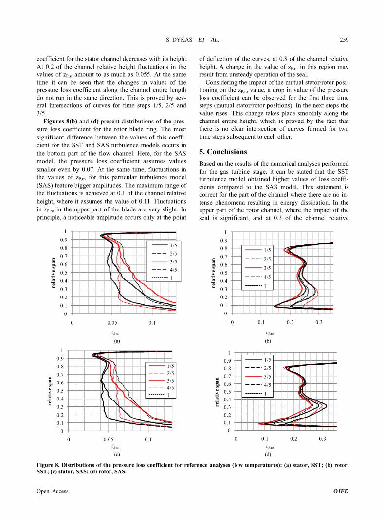
S DYKAS ET AL
Open Access OJFD
259
coefficient for the stator channel decreases with its height At 02 of the channel relative height fluctuations in the values of zPst amount to as much as 0055 At the same time it can be seen that the changes in values of the pressure loss coefficient along the channel entire length do not run in the same direction This is proved by sev- eral intersections of curves for time steps 15 25 and 35
Figures 8(b) and (d) present distributions of the pres- sure loss coefficient for the rotor blade ring The most significant difference between the values of this coeffi- cient for the SST and SAS turbulence models occurs in the bottom part of the flow channel Here for the SAS model the pressure loss coefficient assumes values smaller even by 007 At the same time fluctuations in the values of zPro for this particular turbulence model (SAS) feature bigger amplitudes The maximum range of the fluctuations is achieved at 01 of the channel relative height where it assumes the value of 011 Fluctuations in zPro in the upper part of the blade are very slight In principle a noticeable amplitude occurs only at the point
of deflection of the curves at 08 of the channel relative height A change in the value of zPro in this region may result from unsteady operation of the seal
Considering the impact of the mutual statorrotor posi- tioning on the zPro value a drop in value of the pressure loss coefficient can be observed for the first three time steps (mutual statorrotor positions) In the next steps the value rises This change takes place smoothly along the channel entire height which is proved by the fact that there is no clear intersection of curves formed for two time steps subsequent to each other
5 Conclusions
Based on the results of the numerical analyses performed for the gas turbine stage it can be stated that the SST turbulence model obtained higher values of loss coeffi-cients compared to the SAS model This statement is correct for the part of the channel where there are no in-tense phenomena resulting in energy dissipation In the upper part of the rotor channel where the impact of the seal is significant and at 03 of the channel relative
0
01
02
03
04
05
06
07
08
09
1
0 005 01
rela
tiv
e sp
an
15
25
35
45
1
0
01
02
03
04
05
06
07
08
09
1
0 01 02 03
rela
tive
sp
an
15
25
35
45
1
ζPst ζPro
(a) (b)
0
01
02
03
04
05
06
07
08
09
1
0 005 01
rela
tive
span
152535451
0
01
02
03
04
05
06
07
08
09
1
0 01 02 03
rela
tive
span
15
25
35
45
1
ζPst ζPro
(c) (d)
Figure 8 Distributions of the pressure loss coefficient for reference analyses (low temperatures) (a) stator SST (b) rotor SST (c) stator SAS (d) rotor SAS
S DYKAS ET AL
Open Access OJFD
260
height where an especially big increment in entropy oc- curs the values of the loss coefficients obtained for the SAS turbulence model are higher This probably results from the fact that the turbulent processes taking place in these areas are mapped better by the hybrid Scale-Adap- tive Simulation (SAS) turbulence model
Comparing the two turbulence models attention should also be drawn to the shape of the deflection of the curves in the area at ~03 of the blade relative height Here the curves representing changes in loss coefficients vary mildly for the SST model whereas for the SAS turbu- lence model a considerable refraction of the curves oc- curs Thus the area of high values of the loss coefficient for the SAS model comprises a much smaller part of the channel
Intersections of curves for time steps subsequent to each other were observed for the energy loss coefficient and the pressure loss coefficient calculated for the stator channel This proves that there is a phase shift in the di- rection of the changes in the coefficient value on both sides of the intersection of the curves which leads to a reduced fluctuation in the average value of the loss coef- ficient calculated for the entire channel
For all loss coefficients under analysis the low values in the rotor region correspond to their high values in the region of the stator blade channel This levels out the fluctuations in the values of individual coefficients with- in the entire stage
6 Acknowledgements
The authors would like to thank the Polish Ministry of
Science and Higher Education for the financial support for the research project UMO-201101BST803488
REFERENCES [1] J D Denton ldquoLoss Mechanisms in Turbomachinesrdquo
Journal of Turbomachinery Vol 115 No 4 1993 pp 621-656 httpdxdoiorg10111512929299
[2] N Wei ldquoSignificance of Loss Models in Aerothermody- namic Simulation for Axial Turbinesrdquo Doctoral Thesis Royal Institute of Technology
[3] S Dykas W Wroacuteblewski and H Łukowicz ldquoPrediction of Losses in the Flow through the Last Stage of Low- Pressure Steam Turbinerdquo International Journal for Nu- merical Methods in Fluids Vol 53 No 6 2007 pp 933-945 httpdxdoiorg101002fld1313
[4] P Lampart ldquoInvestigation of Endwall Flows and Losses in Axial Turbines Part I Formation of Endwall Flows and Lossesrdquo Journal of Theoretical and Applied Me- chanics Vol 47 No 2 2009 pp 321-342
[5] W Wroacuteblewski A Gardzilewicz A Dykas and P Ko- lovratnik ldquoNumerical and Experimental Investigation of Steam Condensation in LP Part of Large Power Turbinerdquo Journal of Fluids Engineering Trans ASME Vol 131 No 4 2009 pp 1-11
[6] T P Moffit E M Szanca and W J Whitney ldquoDesign and Cold-Air Test of Single-Stage Uncooled Core Tur- bine With High Work Outputrdquo NASA Report TP-1680 1980
[7] F R Menter ldquoTwo-Equation Eddy-Viscosity Turbulence Models for Engineering Applicationsrdquo AIAA Journal Vol 32 No 8 1994 pp 1598-1605 httpdxdoiorg102514312149
Symbols
loss coefficient h specific enthalpy Jkgminus1 p pressure Pa s specific entropy Jkgminus1Kminus1
ϰ adiabatic exponent
Subscripts
0 stator inlet
1 statorrotor interface 2 rotor outlet En energy rel rotating reference frame ro rotor s entropy st stator t total