numerical analysis and design of upwind sailsaero-comlab.stanford.edu/papers/ssriram.thesis.pdf ·...
TRANSCRIPT

NUMERICAL ANALYSIS AND DESIGN OF UPWIND
SAILS
a dissertation
submitted to the department of aeronautics and astronautics
and the committee on graduate studies
of stanford university
in partial fulfillment of the requirements
for the degree of
doctor of philosophy
Sriram Shankaran
April 2005

c© Copyright 2005 by Sriram Shankaran
All Rights Reserved
ii

I certify that I have read this dissertation and that in
my opinion it is fully adequate, in scope and quality, as
a dissertation for the degree of Doctor of Philosophy.
Antony Jameson(Principal Adviser)
I certify that I have read this dissertation and that in
my opinion it is fully adequate, in scope and quality, as
a dissertation for the degree of Doctor of Philosophy.
Juan J. Alonso
I certify that I have read this dissertation and that in
my opinion it is fully adequate, in scope and quality, as
a dissertation for the degree of Doctor of Philosophy.
Margot Gerritsen
Approved for the University Committee on Graduate
Studies:
iii

To all things alive
iv
Abstract
The use of computational techniques that solve the Euler or the Navier-Stokes equa-
tions are increasingly being used by competing syndicates in races like the Americas
Cup. For sail configurations, this desire stems from a need to understand the influ-
ence of the mast on the boundary layer and pressure distribution on the main sail,
the effect of camber and planform variations of the sails on the driving and heeling
force produced by them and the interaction of the boundary layer profile of the air
over the surface of the water and the gap between the boom and the deck on the
performance of the sail. Traditionally, experimental methods along with potential
flow solvers have been widely used to quantify these effects. While these approaches
are invaluable either for validation purposes or during the early stages of design, the
potential advantages of high fidelity computational methods makes them attractive
candidates during the later stages of the design process.
The aim of this study is to develop and validate numerical methods that solve
the inviscid field equations (Euler) to simulate and design upwind sails. The three
dimensional compressible Euler equations are modified using the idea of artificial com-
pressibility and discretized on unstructured tetrahedral grids to provide estimates of
lift and drag for upwind sail configurations. Convergence acceleration techniques like
multigrid and residual averaging are used along with parallel computing platforms
to enable these simulations to be performed in a few minutes. To account for the
elastic nature of the sail cloth, this flow solver was coupled to NASTRAN to provide
v

estimates of the deflections caused by the pressure loading. The results of this aeroe-
lastic simulation, showed that the major effect of the sail elasticity, was in altering
the pressure distribution around the leading edge of the head and the main sail.
Adjoint based design methods were developed next and were used to induce
changes to the camber distribution of the main sail. The goal of the design process
was to reduce the leading edge suction peaks that were considered to be detrimental
to the growth of the boundary layer. The deflected shape of the sails obtained from
the aeroelastic simulation were used by the design process. The design process re-
sulted in an camber distribution that allowed smooth entry of the flow through the
leading edge of the main sail thereby, reducing the leading edge suction peaks.
vi

Acknowledgments
vii

Contents
iv
Abstract v
Acknowledgments vii
1 Introduction 1
1.1 Design Requirements of Racing Yachts . . . . . . . . . . . . . . . . . 1
1.2 Models of Fluid Flow . . . . . . . . . . . . . . . . . . . . . . . . . . . 3
1.3 Analysis with CFD . . . . . . . . . . . . . . . . . . . . . . . . . . . . 5
1.4 Aeroelastic Analysis . . . . . . . . . . . . . . . . . . . . . . . . . . . 8
1.5 Optimum Design . . . . . . . . . . . . . . . . . . . . . . . . . . . . . 10
1.6 Aerodynamic Shape Optimization . . . . . . . . . . . . . . . . . . . . 12
1.7 Outline of this study . . . . . . . . . . . . . . . . . . . . . . . . . . . 16
2 Discretization of Governing Equations 19
2.1 Overview of the Numerical Scheme . . . . . . . . . . . . . . . . . . . 19
2.2 Finite Volume Discretization of the Flow equations . . . . . . . . . . 21
2.3 Spatial Discretization . . . . . . . . . . . . . . . . . . . . . . . . . . . 23
2.4 Staggered Meshes . . . . . . . . . . . . . . . . . . . . . . . . . . . . . 24
2.5 Implementation of the Cell-Vertex Scheme . . . . . . . . . . . . . . . 29
2.6 Artificial Diffusion . . . . . . . . . . . . . . . . . . . . . . . . . . . . 29
2.7 Analysis of Artificial Compressibility . . . . . . . . . . . . . . . . . . 30
2.8 Time Integration . . . . . . . . . . . . . . . . . . . . . . . . . . . . . 31
viii

2.9 Multigrid Acceleration . . . . . . . . . . . . . . . . . . . . . . . . . . 32
2.10 Parallel Implementation . . . . . . . . . . . . . . . . . . . . . . . . . 35
2.10.1 Domain Decomposition, Load Balancing . . . . . . . . . . . . 35
2.10.2 Parallel implementation of the multigrid algorithm . . . . . . 38
2.10.3 Speedup of the Parallel Implementation . . . . . . . . . . . . . 39
2.11 Governing equations and analysis of the structural model . . . . . . . 39
2.11.1 Structural Model of the Sail . . . . . . . . . . . . . . . . . . . 41
2.12 Aeroelastic Coupling and Mesh Deformation . . . . . . . . . . . . . . 42
3 Analysis of Sail Configurations 46
3.1 Low Mach number, high angle of attack simulations with a compress-
ible flow solver . . . . . . . . . . . . . . . . . . . . . . . . . . . . . . 47
3.1.1 Multi-Element airfoils . . . . . . . . . . . . . . . . . . . . . . 47
3.1.2 Sail simulations . . . . . . . . . . . . . . . . . . . . . . . . . . 47
3.2 Effect of Numerical Discretization and diffusion on artificial compress-
ibility methods . . . . . . . . . . . . . . . . . . . . . . . . . . . . . . 48
3.3 Validation of the parallel implementation . . . . . . . . . . . . . . . . 49
3.4 Single and multi-element sail computations with artificial compress-
ibility methods . . . . . . . . . . . . . . . . . . . . . . . . . . . . . . 50
3.4.1 Characteristics of the main sail . . . . . . . . . . . . . . . . . 50
3.4.2 Characteristics of the Head and Main sail combination . . . . 52
3.5 Aeroelastic simulations for single and multi-element foils . . . . . . . 54
4 Aerodynamic Shape optimization 76
4.1 The general formulation of the Adjoint Approach to Optimal Design . 77
4.2 Adjoint and Gradient formulations . . . . . . . . . . . . . . . . . . . 79
4.2.1 Adjoint Equations for the Euler equations modified by artificial
compressibility method . . . . . . . . . . . . . . . . . . . . . . 83
4.2.2 The need for a Sobolev inner product in the definition of the
gradient . . . . . . . . . . . . . . . . . . . . . . . . . . . . . . 84
4.3 Analysis of the Optimization Procedure . . . . . . . . . . . . . . . . . 86
4.4 Mesh movement . . . . . . . . . . . . . . . . . . . . . . . . . . . . . . 88
ix
4.5 Parallel Implementation . . . . . . . . . . . . . . . . . . . . . . . . . 88
5 Validation of the Optimization Procedure and Results 89
5.1 Shape optimization for airfoils in compressible flow . . . . . . . . . . 90
5.2 Shape optimization of airfoils in incompressible flow . . . . . . . . . . 90
5.3 Three dimensional shape optimization of wings in compressible flow . 95
5.4 Inverse design of wings in incompressible flow . . . . . . . . . . . . . 96
5.5 Inverse design for sail geometries . . . . . . . . . . . . . . . . . . . . 96
6 Conclusions 107
6.0.1 Aerodynamic and Aeroelastic analysis . . . . . . . . . . . . . 107
6.0.2 Aerodynamic design . . . . . . . . . . . . . . . . . . . . . . . 108
Bibliography 110
x

List of Tables
xi

List of Figures
2.1 Dual mesh representation of the control volume . . . . . . . . . . . . 25
2.2 Nodal formulation of the finite volume scheme . . . . . . . . . . . . . 25
2.3 Evaluation of fluxes in three dimensions . . . . . . . . . . . . . . . . 26
2.4 Control volume for cell-vertex schemes in three dimensions . . . . . . 26
2.5 Staggered arrangement of flow variables . . . . . . . . . . . . . . . . . 28
2.6 Half-staggered arrangement of flow variables . . . . . . . . . . . . . . 28
2.7 Interpolation coefficients for use in the multigrid cycle . . . . . . . . . 34
2.8 Transfer of solution, residuals and corrections between the fine and
coarse mesh . . . . . . . . . . . . . . . . . . . . . . . . . . . . . . . . 35
2.9 Domain decomposition of a rectangular region using a bisection method 36
2.10 Halo nodes and the distribution of edges along processor boundaries 37
2.11 Speedup from the parallel implementation . . . . . . . . . . . . . . . 37
2.12 Boundary conditions for the main sail . . . . . . . . . . . . . . . . . . 42
2.13 Boundary conditions for the head sail . . . . . . . . . . . . . . . . . . 43
3.1 Grid and Pressure distribution over a multi-element airfoil geometry
at a M = 0.2 and α = 8.2 degrees . . . . . . . . . . . . . . . . . . . . 56
3.2 Cp distribution at two sections and convergence history of the com-
pressible flow solver . . . . . . . . . . . . . . . . . . . . . . . . . . . . 57
3.3 Potential flow solution from FLO1 at 0,1 and 3 degrees . . . . . . . . 58
3.4 Flow over a NACA 0012 airfoil at 0,1 and 3 degrees using a cell-centered
scheme . . . . . . . . . . . . . . . . . . . . . . . . . . . . . . . . . . . 59
3.5 Flow over a NACA 0012 airfoil at 0,1 and 3 degrees using a nodal scheme 60
xii

3.6 Flow over a NACA 0012 airfoil at 0,1 and 3 degrees using a half-
staggered scheme . . . . . . . . . . . . . . . . . . . . . . . . . . . . . 61
3.7 Total Pressure losses on the airfoil surface at 0o . . . . . . . . . . . . 62
3.8 Total Pressure losses on the airfoil surface at 1o . . . . . . . . . . . . 62
3.9 Total Pressure losses on the airfoil surface at 3o . . . . . . . . . . . . 63
3.10 Total Pressure losses on the airfoil surface at 5o . . . . . . . . . . . . 63
3.11 Sail geometry . . . . . . . . . . . . . . . . . . . . . . . . . . . . . . . 64
3.12 Pressure distributions along sections at 1, 25 and 85 percent of the
height of main sail . . . . . . . . . . . . . . . . . . . . . . . . . . . . 65
3.13 Spanwise force distributions . . . . . . . . . . . . . . . . . . . . . . . 66
3.14 Variation of Lift and Drag with wind incidence . . . . . . . . . . . . . 66
3.15 Effect of mast on variation of Lift and Drag with wind incidence . . . 67
3.16 Effect of heeling angle on variation of Lift and Drag . . . . . . . . . . 67
3.17 Twist,camber and chord distribution of the head sail . . . . . . . . . 68
3.18 Twist,camber and chord distribution of the main sail . . . . . . . . . 68
3.19 Pressure distributions along sections at 1, 25 and 85 percent of the
height of head sail . . . . . . . . . . . . . . . . . . . . . . . . . . . . . 69
3.20 Pressure distributions along sections at 1, 25 and 85 percent of the
height of the main sail . . . . . . . . . . . . . . . . . . . . . . . . . . 70
3.21 Spanwise force distributions on the head sail . . . . . . . . . . . . . . 71
3.22 Spanwise force distributions on the main sail . . . . . . . . . . . . . . 71
3.23 Pressure distribution over the pressure and suction side of the head
and sail combination . . . . . . . . . . . . . . . . . . . . . . . . . . . 72
3.24 Original and deformed sail sections for the head sail . . . . . . . . . . 73
3.25 Original and deformed sail sections for the main sail . . . . . . . . . . 73
3.26 Pressure distributions along sections at 1, 25 and 85 percent of the
height of head sail after aeroelastic analysis . . . . . . . . . . . . . . . 74
3.27 Pressure distributions along sections at 1, 25 and 85 percent of the
height of main sail after aeroelastic analysis . . . . . . . . . . . . . . 75
5.1 Comparison of the gradients from SYN75 and SYN82 . . . . . . . . . 91
xiii
5.2 Comparison of the first co-state variable from SYN75 and SYN82 . . 91
5.3 Comparison of the second co-state variable from SYN75 and SYN82 . 92
5.4 Comparison of the third co-state variable from SYN75 and SYN82 . . 92
5.5 Comparison of the fourth co-state variable from SYN75 and SYN82 . 93
5.6 Initial pressure distribution for the RAE-2822 airfoil . . . . . . . . . . 93
5.7 Drag minimization for the RAE-2822 airfoil . . . . . . . . . . . . . . 94
5.8 Final and target pressure distribution for the RAE-2822 airfoil . . . . 94
5.9 Initial and final pressure distribution, o is the target pressure distribu-
tion, x is the computed pressure distribution for the redesigned airfoil 95
5.10 Initial and final pressure and section geometries . . . . . . . . . . . . 97
5.11 Initial and final pressure distributions at 5 %, 50 % and 95 % of the
wing span . . . . . . . . . . . . . . . . . . . . . . . . . . . . . . . . . 98
5.12 Initial pressure distribution over a NACA 0012 wing . . . . . . . . . . 99
5.13 Final pressure distribution and modified section geometries along the
wing span . . . . . . . . . . . . . . . . . . . . . . . . . . . . . . . . . 100
5.14 Final computed and target pressure distributions at 0 % and 20 %of
the wing span . . . . . . . . . . . . . . . . . . . . . . . . . . . . . . . 101
5.15 Final computed and target pressure distributions at 40 % and 60 % of
the wing span . . . . . . . . . . . . . . . . . . . . . . . . . . . . . . . 101
5.16 Final computed and target pressure distributions at 80 % and 100 %
of the wing span . . . . . . . . . . . . . . . . . . . . . . . . . . . . . 102
5.17 Final computed and target pressure distributions at 0, 25, 75 and 100 %
of the wing span at 3 degrees angle of attack . . . . . . . . . . . . . . 103
5.18 Initial (o) and final(+,x) pressure distribution at 15, 32, 75 and 85%
height on the main sail . . . . . . . . . . . . . . . . . . . . . . . . . . 105
5.19 Initial and redesigned camber line at 15,32,75 and 85% of height . . . 106
6.1 Components of the overall design process for upwind sails . . . . . . . 109
xiv

Chapter 1
Introduction
1.1 Design Requirements of Racing Yachts
Races like the Americas Cup have seen significant improvements in the designs of both
the hull and the sails over the last two decades. Competing syndicates are constantly
pushing the aerodynamic and structural limits of the designs as improvements of less
than 0.5 % in the speed of the boat result in savings of around 25-35 seconds, which
is near the margin of victory for these races. For the windward leg of the race, a good
measure of the performance of a design is the distance that the boat travels directly
to windward in a given time. This performance index (called the speed-made-good by
the boat) is dependent on both the speed of the boat and the true sailing course, which
in turn are dependent on the aerodynamic and hydrodynamic forces produced by the
sails and the hull. In general, the windward performance of the boat can be improved
by reducing the resistance of the hull and the drag of the sails. However changes in
the aerodynamic and hydrodynamic forces alter the equilibrium of the sail boat which
then has to adjust its speed. Hence, the design of sailing yachts has to be carried out
in an environment where the analysis and design procedures for the sails and the hull
are integrated to realize a meaningful overall design. Traditionally, designers have
used Velocity Prediction Programs (VPP) which essentially solve for the equations
of equilibrium of the boat. These programs typically estimate the aerodynamic and
hydrodynamic forces using simple potential flow solvers. These provide quick answers,
1

CHAPTER 1. INTRODUCTION 2
enabling the designer to evaluate a wide array of designs. However, there exists large
regions of rotational flow and significant viscous interaction, where the assumptions
of potential flow are not valid. Hence there exists the need to develop and validate
alternate design techniques using more realistic models of the flow.
There exist a variety of tools that a designer can exploit to make improvements
to an existing design. Experimental techniques have been a favorite choice with most
designers and have been used successfully for downwind designs. This method intro-
duces no approximations to the physical properties of the fluid, and hence carefully
performed wind-tunnel tests can provide good estimates of the aerodynamic and hy-
drodynamic forces developed by the sail boat. However, experimental facilities are
usually expensive to build and maintain and have slower turn-around times than
computational models. For sail geometries, experimental testing usually does not
provide the designer with detailed descriptions of the pressure and velocity over the
sail geometry, as it is difficult to mount sensors that do not interfere with the flow
physics. Hence, experimental methods can usually only provide macroscopic esti-
mates of quantities of interest. Further, the twist in the onset profile of the wind
and the interaction of the free-surface with the hull are difficult to accurately model
through experimental methods. Over the last decade, experimental facilities in New
Zealand, California and Italy have been built that allow for twisted onset flow. Es-
timates of the flying shape of the sail and the variation of sail shape and trim for
varying weather conditions are typically observed using cameras mounted along the
sail and colored ribbons at various positions along the height of the sail.
Alternatively, computational models are finding increasing acceptance within the
sailing community [1]. Computational models have the capability of providing de-
tailed estimates of the aerodynamic and hydrodynamic forces along with deflections
developed by the sail. The steadily decreasing cost of computational simulations
is making this option more attractive than experimental methods during the initial
stages of design. Computational Fluid Dynamics (CFD) uses numerical solution pro-
cedures for mathematical models that describe the evolution of the flow-field. Hence,
it is possible to obtain solutions to a hierarchy of mathematical models that can be
used to continuously refine an initial design. Linear potential flow models are used by
CHAPTER 1. INTRODUCTION 3
many sail designers to estimate the forces produced by the sails and the hull. These
models are easy to implement and are computationally inexpensive while providing
the designer with valuable insights during the early stages of the design process. How-
ever, these models do not account for rotational flow fields and neglect viscous effects.
Rotational effects can be modeled by the full Euler equations of inviscid flow. For
upwind sail configurations an inviscid fluid model is valid for angles of attack up to
20 degrees provided there is no significant separation along the trailing edge, and the
sails have been trimmed so that leading edge separation is not too large either. These
models have the potential to accurately predict the induced drag which typically ac-
counts for 15 % of the total drag. The development of computational tools that solve
the Euler equations could also lay the foundation for the introduction of viscous ef-
fects either by solving the Navier-Stokes equations or by coupling a boundary layer
solution to the inviscid solution.
The key requirements for effective computational tools are
• sufficient accuracy
• acceptable computational cost
• rapid turn around
• reliability
• procedures to optimize the design.
The issues which need to be addressed in order to satisfy these requirements are
examined in more detail in the next sections leading to an outline of the thesis in
Section 1.7.
1.2 Models of Fluid Flow
There exist a variety of mathematical models for the flow-field that have been used
by the aerodynamic community. The most general description of the behavior of the
fluid particles involves descriptions of the time-evolution of fluid properties and are
CHAPTER 1. INTRODUCTION 4
described by the Boltzmann’s equations. It is easy to see that such particle-based
formulations quickly become intractable for all but the simplest flows due to the large
number of particles that need to simulated, and also the lack of universal physical
models to account for the interaction of various fluid particles.
Simplifying assumptions to the Boltzmann equations lead to the Navier-Stokes
equations which been found to consistently provide accurate descriptions of the flow
features for a variety of flow regimes. The flow around upwind and downwind sails and
around the hull/keel/appendages occur at high Reynolds numbers and hence, they
are turbulent in nature. The range of length and time scales present in turbulent flows
pose considerable difficulty both in the mathematical formulation and the numerical
resolution of the observed phenomena. Various models to predict the evolution of
the turbulent structures and the turbulent eddy viscosity have been developed for a
range of fluid flows. Direct Numerical Simulations that rely on the solution of the
Navier-Stokes equations in their original form, try to resolve all the scales associated
with turbulence. Due to the large range of scales involved with turbulence, these
methods have only been used for simple geometries to reduce the computational cost
of the simulation, mostly with the aim of gaining better insights into the physics
of turbulence. Alternatively, Large Eddy Simulations resolve some of the turbulent
scales while modeling the others. These have allowed more complex geometries to be
analyzed, but they are still prohibitively expensive for use in an industrial setting.
Consequently the Reynolds Averaged Navier-Stokes equations are generally used for
industrial simulations. The major stumbling block with this approach is the need for
models to predict the evolution of the turbulent quantities. Turbulence models for
the particular problem at hand have to be tested and tuned to arrive at meaningful
estimates of the quantities of interest. The quest for a universal turbulence model
is ongoing and until significant inroads are made in this area, engineers are left with
models that exhibit drastically different behavior for different flow regimes.
A further approximation that eliminates the viscous terms from the governing
equations, leading to the Euler equations, allows for the fluid to be compressible or
incompressible and the flow to be rotational or irrotational. Accordingly this set of
equations is capable of providing better estimates than the potential flow solvers.

CHAPTER 1. INTRODUCTION 5
Further, the twist in the onset flow can be also be easily included in the bound-
ary conditions for the Euler equations. The routine use of inviscid calculations in
the aeronautical world has resulted in well established numerical and computational
techniques. Analysis of shock structures in transonic and supersonic flight has led to
a wide array of computational schemes embedded in Finite Volume, Finite Element
and Finite Difference techniques with various flavors to identify the shock structures
and pressure distributions around airfoils, wings and complete aircraft configurations.
Significant developments in the numerical analysis of the Euler equations has resulted
in fast solvers that use multigrid and residual averaging techniques along with effi-
cient time-stepping algorithms to advance the solution very rapidly to a steady state.
Space discretizations techniques are also well understood, and can provide level of
accuracy needed for engineering estimates. Growth in computing power has added
fuel to the development of this technology, and the routine use of parallel computing
techniques has reduced the computational time of inviscid analysis to the order of a
few minutes. Hence, inviscid flow models can been incorporated into the design cycle
to replace potential flow solvers in the design process.
1.3 Analysis with CFD
Discretization of the flow equations requires the subdivision of the computational
domain into a grid of sufficiently small cells. The first choice to be made is the type
of grid.
Numerical solutions to the governing partial differential equations of fluid flow
were first obtained using computational grids that were structured in nature. It is
easy to obtain higher order accurate flow solutions and boundary conditions with
these grids and hence a wide variety of numerical techniques have been developed
for structured grids. However, for complex geometries, the generation of body-fitted
structured grids is not straight-forward. Structured grid generation techniques have
reached a state of considerable maturity, but typical turn-around times of the grid
generation process are still of the order of weeks, or even months. Unstructured grid
generation techniques that divide the computational domain into arbitrary polyhedral

CHAPTER 1. INTRODUCTION 6
elements can handle complex geometries with greater ease than structured grids.
They also have the potential to be automated, and hence might be incorporated in
a design environment where repeated changes to the geometry have to be performed
while the design evolves.
Over the last two decades well established grid generation techniques for unstruc-
tured grids have been developed. The Delaunay criterion and the advancing front
technique are two of the most widely used techniques by these researchers. While
the use of the Delaunay criterion results in meshes of the highest possible mesh qual-
ity for a given distribution of mesh points, the advancing front algorithm allows the
user more control over point-placement within the computational domain. However,
unstructured grid generation techniques for viscous flows have not yet reached the
maturity that allows them to be completely automated. Nevertheless, a variety of
grid generation methods for both structured and unstructured grids has alleviated
the problem of grid generation, and it is now possible to produce structured and
unstructured grids for very complex geometries.
The nature of unstructured grids lends itself naturally to Finite Volume and Finite
Element methods. Depending on the nature of the underlying discretization, either
the elements of the unstructured grid or the dual of the mesh can be used to construct
non-overlapping control volumes around each computational node. A reconstruction
of the fluxes along the edges of the control volume along with artificial dissipation
terms to prevent odd-even coupling can be shown to be identical to a Finite Element
approximations with linear basis functions and a compact stencil spanning the control
volume. Some of the first calculations over a complete aircraft configuration were
performed with a finite volume technique of this type which was mathematically
presented as a Finite Element method [28].
Spatial discretization of the convective terms of the governing equations along
with the numerical diffusion terms results in a set of ordinary differential equations
that can be integrated in time to obtain time accurate and steady state flow solutions.
These ODEs can be integrated explicitly using a multistage Runge-Kutta scheme with
an appropriate choice of coefficients that maximize the stability of the time evolution.
To accelerate convergence to steady state, multigrid and residual averaging techniques

CHAPTER 1. INTRODUCTION 7
can be used.
The best choice of coarser grids for unstructured multigrid schemes is still an open
problem. Generating a series of meshes repeatedly from a grid generator, edge col-
lapsing techniques which ‘contract’ a given mesh, and agglomeration methods which
fuse cells from a given mesh are three approaches that have been tried. Generating
the meshes repeatedly from a grid generator places a considerable burden on the
grid generator, and is not easy to incorporate in an automated procedure. Further,
the need to transfer the solution and the residuals to coarser meshes and the correc-
tions to a finer mesh necessitates fast algorithms to locate points within cells. Edge
collapsing algorithms use heuristic ideas to repeatedly collapse edges from a given
mesh. It is possible to automate this procedure to generate coarser meshes from a
given fine mesh. Further, this method has the advantage of being able to compute
the interpolation coefficients for the multigrid while the coarser meshes are gener-
ated thereby avoiding the need to use additional search algorithms. Agglomeration
multigrid techniques ‘fuse’ cells from a given mesh to generate the coarser meshes.
This gives rise to cells on the coarser meshes which have arbitrary shape and hence
require efficient data structures to implement the underlying numerical schemes on
them. While the coarser meshes are obtained using a set of heuristic ideas, it is also
possible to automate this procedure. Further the coefficients for the multigrid cycle
are automatically obtained during the agglomeration cycle and the flux balances on
the coarser meshes can be free of any interpolation errors. Further research is needed
to determine whether agglomeration is superior to edge collapsing, or whether some
other technique can yield a faster rate of convergence.
Spatial discretization of the convective terms of the governing equations along
with the numerical diffusion terms results in a set of ordinary differential equations
that can be integrated in time to obtain time accurate and steady state flow solutions.
These ODEs can be integrated explicitly using a multistage Runge-Kutta scheme with
an appropriate choice of coefficients that maximize the stability of the time evolution.
To accelerate convergence to steady state, multigrid and residual averaging techniques
can be used.
The above mentioned numerical algorithms are widely used in the aerodynamic
CHAPTER 1. INTRODUCTION 8
design of aircraft by most commercial civil transport manufacturers across the world.
They were designed to treat compressible flows with embedded shock structures.
However, in the incompressible limit they require some modifications. Chorin [30]
proposed the idea of artificial compressibility to enable the re-use of the well developed
numerical techniques for compressible flows for incompressible flows. The key idea
of this method is to augment the continuity equation by a time dependent pseudo-
pressure term. While the value of this pressure is not physically meaningful during
the evolution of the system of equations, in the steady state it provides the pressure
which satisfies the momentum equations, and it drops out of the continuity equation,
thereby satisfying both the continuity and momentum equations simultaneously. This
idea has been used by a number of researchers [3], [4], [31] to convert computational
programs developed for compressible flows to handle incompressible flows and has
proven to be robust and accurate for steady state problems.
1.4 Aeroelastic Analysis
The pressure distribution acting on a lifting surface is determined by its shape and
in most aerodynamic applications this shape is fixed under the assumption that the
geometry does not change appreciably under the action of the aerodynamic loads.
However, this is not the case when the lifting surface is an elastic membrane like a sail,
since the twist and camber of such wings under the load may be quite different from
their unloaded values. The flexible behavior of sails necessitates the need to perform
aeroelastic simulations with analysis methods which can treat large displacements.
Classical models to study the behavior of membranes under static and unsteady loads
have been extensively studied. In applications to sails, the structural analysis needs to
take into account geometric nonlinearities. However, since the strains remain small,
constitutive laws for the material can be considered to be linear, with the result that
the tension in the structure is a linear function of the local deformation.
Charvet [5] presented a scheme to estimate the steady equilibrium configuration of
a sail. This analysis decomposed the large displacements into two steps. The first step
computed the large displacements of an inextensible sail and the second considered the

CHAPTER 1. INTRODUCTION 9
elastic displacements of an elastic sail. This approach is satisfactory for structures
whose Young’s modulus is large thereby limiting the elastic deformations to small
displacements. Another approach, pursued in the works of Jackson et. al. [6] and
Fukusawa et. al. [7], considered small displacements to an arbitrary elastic structure.
Large-displacement analysis of an elastic membrane is an ongoing quest [24], [25] and
no satisfactory analysis has been performed to date.
Another important feature of the structural deformations induced in sail geome-
tries by the aerodynamic loading is the possibility of wrinkles which are usually local
in their presence. Due to the highly non-linear nature of the formation of these
wrinkles, most sail designers have neglected the effect of these wrinkles. Studies by
Miller et. al. [8], [9], argued that the most important effect of wrinkles is to locally
increase the average strain in the normal direction due to a strain or displacement in
the longitudinal direction. Under these assumptions, they accounted for wrinkles by
locally increasing the Poisson’s ratio in regions where wrinkles are formed and using
the Hookean material properties which now become dependent on the local state of
strain. This approximate theory attempts only to estimate the average wrinkle strain,
and does not identify the shape of the wrinkle. Further, the emergence of wrinkles
is based on generalized assumptions originating from the magnitude of the principal
strain in each element of the finite element model.
Another important feature of modern day rigs for races like the Americas Cup is
the flexibility of the mast. The masts tend to be flexible to exploit the advantages
of automatic shape changes under heavy wind conditions. Studies which account for
the flexibility of the mast usually employ an incremental procedure, where the sail
and the mast are deflected in turn with appropriate boundary conditions along the
point of attachment [21], [23], [22]. An integrated structural simulation of a complete
sail rig has still not been reported in the open literature, and could be invaluable in
the quest to achieve improved designs.
CHAPTER 1. INTRODUCTION 10
1.5 Optimum Design
The search for optimal designs that maximize/minimize a performance index has been
the aim of designers in all engineering disciplines. Identification of a possible set of
design variables that have the maximum influence on the performance of a design
along with suitable representations of the state of the system are needed to cast the
optimization problem in a mathematical frame-work. Typical design problems in most
engineering fields are multi-disciplinary in nature. The design of sails boats is multi-
disciplinary due to the tightly coupled interaction between the sails and hull. Within
this multi-disciplinary environment, it is possible to identify optimization problems
that are confined to a single discipline provided the constraints from other disciplines
are satisfied. Aerodynamic shape optimization is one such area that involves the
identification of an optimum shape to improve the aerodynamic characteristics of the
design. It is possible to cast the problem of identifying an optimum sail, hull or keel
geometry under this umbrella. If the drag of a given sail shape has to be reduced,
the span loading has to be altered. However, altering the span loading changes the
heeling moment and the equilibrium of the boat and hence suitable constraints have
to be provided to achieve a meaningful design. On the other hand, it is often desirable
to determine a sail shape that provides a favorable pressure distribution that inhibits
separation of the boundary layer. While this class of optimization problems (herein
referred to as shape optimization problems) can be studied within the single discipline
of aerodynamics, a major difficulty is the large dimensionality of the design space.
To overcome this problem, sail designers typically optimized a given design using a
combination of parametric studies [2] and experience.
The task of locating minima in the design space requires some knowledge of the
topology (typically slope/gradient and curvature information) of the design space and
a ‘search’ algorithm that navigates through the design space to a minima. Due to the
complexity of the problem many attempts have been based on techniques which do
not explicitly compute the gradients in the design space. Some of these approaches
use evolution or genetic algorithms to evolve the design towards an optimum. These
algorithms use a collection of candidate designs that are then modified using heuristic

CHAPTER 1. INTRODUCTION 11
rules based on some knowledge of the design space to identify a new set of designs.
An advantage of these approaches is that they are relatively easy to implement and
do not usually require gradient evaluations. However, their computational complexity
can become prohibitive with a large number of design variables. Hence, successful
optimization has required an experienced user to judiciously select a minimal set of
design functions which adequately defines the design space in which the search for
the optimum navigates.
Alternately, first order gradient based methods estimate the first derivative of
the change of the cost function with respect to the choice of design variables. This
estimate of the gradients is then used to predict a new design configuration that leads
to an improvement in the performance index. The main challenge for this approach is
to estimate the gradients accurately and cheaply. Initially, finite-difference methods
were used to estimate the gradient of the cost function with respect to the design
variables. Hence, these methods require one or two flow solutions to obtain the
gradient with respect to each design variable. The formulation of the optimization
problem in a control theory context leads to the idea of adjoint systems which allow
evaluation of the gradients with respect to a large number of design variables with
minimal computational effort. While the complexity of this approach scales with the
number of performance indices, this is not a difficulty for aerodynamic design as the
primary performance measures are lift and drag.
Once the gradients have been evaluated a variety of algorithms can be used to
evolve the design. The simplest method, called the steepest descent method, takes
a step in the direction of the negative gradient. Hence, this approach requires an
estimate of the step-size which is usually obtained by trial and error. Alternatively,
Newton methods make use of the curvature of the topology and the slope to navigate
through the design space have also been used. These methods require estimates of
the second derivative of the cost function with respect to the design variables, and
again can quickly become expensive or intractable. Under these circumstances the
use of adjoint based design methods combined with the steepest descent technique
has proven to be a good compromise which provides a robust and efficient tool for
aerodynamic shape optimization, as described in the next section.

CHAPTER 1. INTRODUCTION 12
1.6 Aerodynamic Shape Optimization
Aerodynamic shape design has long been a challenging objective in the study of fluid
dynamics. CFD has played an important role in the aerodynamic design process since
its introduction for the study of fluid flow. However, CFD has mostly been used in
the analysis of aerodynamic configurations in order to aid in the design process rather
than to serve as a direct design tool in aerodynamic shape optimization. Although
several attempts have been made in the past to use CFD as a direct design tool, it has
not been until recently that the focus of CFD applications has shifted to aerodynamic
design [42, 43, 44, 45, 46, 47]. This shift has been mainly motivated by the availability
of high performance computing platforms and by the development of new and efficient
analysis and design algorithms. In particular, automatic design procedures which use
CFD combined with gradient-based optimization techniques, have made it possible
to remove difficulties in the decision making process faced by the aerodynamicist.
Gradient-based optimization techniques typically identify a control function to be
optimized and a suitable cost function whose optimum location in the design space
is the quest of the algorithm. The control function can either be parameterized to
reduce the number of design variables or represented in forms which account for all
possible variations subject to applicable constraints. To determine future designs
within a design space, estimates of the slope in the design space are evaluated and an
algorithm to determine possible movement within the design space is used to move
towards a better/optimum design. Finding a fast and efficient way to determine the
gradients is critical to this method as is the need for an intelligent search algorithm.
Gradient information can be computed using a variety of approaches. The finite-
difference method is probably the most straight-forward way of computing these gra-
dients. In the finite-difference method, small steps are taken in each and every one of
the design variables independently, in order to find the sensitivity of the cost function
with respect to those design variables. Since each of these steps requires a complete
flow solution, the computational cost of this method is proportional to the number
of design variables, and, consequently, it cannot be afforded for problems with design
spaces of large dimensionality. Further, the accuracy of the gradients is sensitive to

CHAPTER 1. INTRODUCTION 13
the choice of the step used to perturb each design variable which can be alleviated by
alternative methods whose accuracy is independent of the choice of step size, such as
the complex step method [59] and automatic differentiation [60].
As an alternative choice, the control theory approach has dramatic computational
cost advantages when compared to any of these methods. The foundation of con-
trol theory for systems governed by partial differential equations was laid by J.L.
Lions [48]. The control theory approach is often called the adjoint method, since
the necessary gradients are obtained via the solution of the adjoint equations of the
governing equations of interest. The adjoint method is extremely efficient since the
computational expense incurred in the calculation of the complete gradient is effec-
tively independent of the number of design variables. The only cost involved is the
calculation of one flow solution and one adjoint solution whose complexity is similar
to that of the flow solution. Control theory was applied in this way to shape design
for elliptic equations by Pironneau [50] and it was first used in transonic flow by
Jameson [42, 43, 51]. Since then this method has become a popular choice for design
problems involving fluid flow [45, 52, 53]. In fact, the method has even been success-
fully used for the aerodynamic design of complete aircraft configurations [44, 54].
Gradient formulations which require the solution of an adjoint system have fallen
into the categories of the discrete and continuous approaches. In the former, the
adjoint system to the discretized flow equations are assembled to obtain the gradient,
thereby necessitating the need to the formulate different adjoint systems for different
discretizations. In the latter, the adjoint system to the original flow equations in
partial difference form is used to estimate the gradients eliminating the need to refor-
mulate the adjoint equations. Studies by Siva Nadarajah and Jameson [49] concluded
that there is no particular benefit in using either one of these methods due to the
trade-offs between the complexity of the discretization of the adjoint equations for
the continuous and discrete approaches, the accuracy of the resulting estimates of the
gradient, and the computational costs required by each method to reach an optimum.
Jameson and Vassberg also compared discrete adjoint versus continuous gradients for
the Brachistochrone problem in which an exact optimal solution is known and showed
that in this case the continuous gradient is slightly more accurate [55].

CHAPTER 1. INTRODUCTION 14
Jameson’s initial work and Jameson and Reuther’s later works are based on the
continuous adjoint method. Anderson and Venkatakrishnan explored the continuous
adjoint on unstructured grids [53]. Anderson and Nielsen have also implemented the
discrete adjoint on unstructured grids [57]. In their work, Anderson et al. presented
the accuracy of the adjoint sensitivity derivatives in aerodynamic design using the
Navier-Stokes equations, and also presented some design examples including a wing
drag minimization and an inviscid multi-element airfoil shape design.
Using the control theory approach it is possible to obtain Frechet derivatives
of the cost function for a set of design variables which allow for the all possible
shapes of the control surface in question, usually a wing or a sail geometry. This
approach mandates the use of all the computational points in the mesh that represent
the control surface and hence could be in the order of a few thousand. Estimating
gradients for these design variables can quickly become expensive if intelligent choices
on the mesh perturbation and gradient calculations are not made. A recent study
by Jameson and Sangho Kim [73] has enabled gradient calculations to eliminate this
need by rewriting the formulations in terms that depend only on the flow and adjoint
solution on the control surface. This finding has far reaching implications to the
world of design using unstructured grids. Earlier formulations of the gradients under
the umbrella of adjoint methods required mesh displacement strategies and residual
evaluations for perturbations in each design variable. While it is possible to arrive
at efficient choices to perform this on structured grids, the lack of structure with
unstructured grids requires intelligent mesh perturbation techniques. Hence earlier
researchers with unstructured grids used a parametric representation of the control
surface. This reduced set of design variables might be incapable of recovering all
possible shapes. The use of the reduced gradient formulation eliminates this difficulty
and allows the designer to view the shape as a free surface.
For the class of aerodynamic shape optimization problems which are investigated
in this study, the design space is essentially infinitely dimensional. The problem is
one of choosing an optimum curve or curved surface, as in classical problems in the
calculus of variations and trajectory optimization. Suppose that the performance
is measured by a cost function I which depends on a function y(x), where under a

CHAPTER 1. INTRODUCTION 15
variation δy(x), the variation of the cost is δI.Now suppose that δI can be expressed
to first order as
δI =
∫G(x)δy(x)dx, (1.1)
where G(x) is the gradient. Then by setting
δy(x) = −λG(x), (1.2)
one obtains an improvement
δI = −λ∫G2(x)dx, (1.3)
unless the gradient is zero. Thus the vanishing of the gradient is a necessary condition
for a local minimum.
In order to accelerate the search, one may resort to using the Newton method.
Here, the search direction is based on the equation represented by the vanishing of
the gradient and is solved by the standard Newton iteration for nonlinear equations.
Suppose that the Hessian is denoted by
A =∂G∂y, (1.4)
then the result of a step δy may be linearized as
G(y + δy) = G(y) + Aδy. (1.5)
This is set to zero for a Newton step; therefore
δy = −A−1G. (1.6)
The Newton method is generally effective if the Hessian can be evaluated accurately
and cheaply.
Quasi-Newton methods estimate A or A−1 from the changes of the gradient
recorded during successive steps. For a discrete problem, it requires N steps to

CHAPTER 1. INTRODUCTION 16
obtain a complete estimate of the Hessian. Therefore, as the dimensionality of the
design space increases, this method requires in more memory to compute the Hessian
and more steps to reach an optimum. This motivates the search for an alternative.
Steepest descent methods provide an alternative search scheme. Here a step is
taken in the negative gradient direction. Denoting the iterations with the superscript
n, we have
yn+1j = yn
j − λGnj . (1.7)
This may be regarded as a forward Euler discretization of a time dependent process
with λ = ∆t. Hence,∂y
∂t= −G. (1.8)
The simplicity of steepest descent methods is off-set by the need to identify step
sizes and the potentially large number of steps that might be required to reach an
optimum. However, for typical cost functions of interest in aerodynamic problems,
the design space seems to be rather benign, with the result that steepest descent
methods provide accurate answers.
1.7 Outline of this study
The first part of the thesis describes the development of the analysis tool aimed at
providing a viable alternative to linear potential flow models. Towards this objective,
the flow solver has to be both robust and have fast turn-around times. In this study,
the numerical solution procedure that simulates the flow around the sails uses a dis-
cretization of the computational domain into unstructured tetrahedra and hence, it
can easily be extended to include the geometry of the deck and the hull in the anal-
ysis. Simulations of the hull-appendages can also be performed using unstructured
grids and eventually it would be possible to couple the sail simulations with the hull
calculations to provide an integrated analysis tool.

CHAPTER 1. INTRODUCTION 17
Finite Volume techniques in conjunction with unstructured grids are used to dis-
cretize the governing equations of motion of an incompressible flow equations. Spa-
tially second order accurate schemes with numerical diffusion and multistage Runge-
Kutta time integration schemes are used to advance the solution to a steady state.
Non-nested multigrid methods, where the meshes are regenerated, along with implicit
residual averaging techniques are used to obtain converged solutions in about 75-100
multigrid cycles. The algorithm is parallelized to reduce turn-around time of the
simulations to the order of a few minutes. To predict the flying shape of sails, this
flow solver is coupled to the commercial structural analysis package, NASTRAN.
Using this tool, the variations of the lift and drag for different wind and sail setting
is studied. Multiple sail geometries are also analyzed to study the interaction of the
main sail with the genoa.
The second part of the thesis addresses the quest for optimum sail design. Here
the aerodynamic shape optimization problem is cast under the control theory ap-
proach. Accordingly the shape of the sail is identified as the control mechanism that
is modified to meet the required performance criteria. Hence, an adjoint system to
the governing flow equations is introduced and solved using the same techniques as
those used for the flow solver. Gradient formulations which use the solution to an
adjoint system are used together with steepest descent search methods to identify an
optimum in the design space. Each point in the computational mesh that describes
the sail geometry is used to alter the sail shape, thereby allowing all possible shapes
to be recovered during the optimization procedure. Gradient formulations which de-
pend only the surface geometry information have largely made possible the use of
unstructured grids in this design methodology as they eliminate the contribution of a
field integral to the gradient formulation. This field integral is typically computed by
perturbing each design variable and computing a new residual at each mesh point in
the computational mesh proving to be quite expensive for design variables which run
in the order of a few thousand. Shape modifications to an existing design are made
to improve the performance of the design. In this study, inverse problems are inves-
tigated where the target pressure distribution is prescribed through a combination of
experience and engineering intuition.
CHAPTER 1. INTRODUCTION 18
In the next two chapters, the numerical implementation of the analysis tool is
discussed with emphasis on the discretization of the fluid-flow equations. To make
more realistic predictions an aeroelastic package is used to predict the flying shape of
the sail. This aeroelastic package is used to analyze a head and main sail geometry
that is representative of those used in the Americas Cup. In the last two chapters
the design philosophy is laid out with particular reference to the gradient calculations
on unstructured grids. Results for an inverse design exercise are provided to validate
the design process, and then it is used to alter the shape of the sails to eliminate
undesirable flow features.

Chapter 2
Discretization of Governing Fluid
and Structural Equations
2.1 Overview of the Numerical Scheme
Traditionally, panel methods with corrections to account for the boundary layer and
wake have been used to model the fluid flow around sails [10], [14]. For most en-
gineering purposes, these simplified linear potential flow models provide reasonably
accurate estimates of the forces and moments on upwind sails, and they have been
exclusively used by sail designers over the last couple of decades [11], [15], [16], [17].
However, the flow around sails possess substantial regions of rotation, the most com-
mon feature being the shedding of vorticity from sharp edges. With a potential flow
model, the user is required to set up vortex-sheet discontinuities in the flow field and
then ‘adjust’ and ‘fit’ them to the surrounding flow. This requires prior knowledge
of where the sheets begin, and becomes complicated for all but the simplest situa-
tions. However, potential flow codes have been successfully used in Americas Cup
campaigns and continue to the mainstay of most designers.
Further, the desire to incorporate the effect of twist in the onset flow and viscous
phenomena necessitate the use of more advanced numerical models that solve the
complete field equations. However, these non-linear models require the solution of
the coupled partial differential equations governing the evolution of the fluid which
19

CHAPTER 2. DISCRETIZATION OF GOVERNING EQUATIONS 20
are much more computationally expensive than panel methods. Advances in both
numerical techniques and the growth in computing power over the last two decades
have alleviated these problems. The use of parallel computing techniques along with
the use of multigrid and residual averaging techniques have enabled flow solutions to
be performed in the order of minutes [27]. Thus, it is possible to obtain numerical
solutions to the field equations with turnaround times that are acceptable to the
overall design process while allowing for non-linear models to be incorporated in the
design process. The solution to the structural equations, static and time-dependent,
has been extensively studied and have reached a stage of considerable maturity such
that routine analysis can be performed without much intervention by the end-user.
Commercial finite element packages provide a range of options to handle linear and
non-linear deformations under a variety of operational conditions. These methods
have the robustness and flexibility needed for analysis and design.
This chapter discusses the numerical scheme used to solve the governing equations
for both the fluid and the structure. The governing equations of motion of a com-
pressible inviscid fluid are modeled using the Euler equations, modified using the idea
of artificial compressibility to handle incompressible flows. In the following sections
the finite volume approach to discretize the governing equations on an unstructured
grid are presented, along with Runge-Kutta time integration techniques and residual
averaging and multigrid methods. The combined use of these techniques enables a
flow solution to be obtained in about 75-100 multigrid cycles. Further, the use of
parallel computing methods reduce the cost of these computations to the order of a
few minutes. The pressure loads obtained from the fluid solver are fed to a structural
analysis program to estimate the deflections. Because of the large deflections typi-
cally observed in sail geometries, a non-linear model provided by NASTRAN is used
within the structural solver. This non-linear model breaks the loading into a series of
small steps, which are applied sequentially. The deflected shape is used to modify the
computational mesh for the flow solver, using standard mesh deformation techniques
in order to obtain a new pressure loading. Finally an iterative process that couples
the flow and structural solver is used to arrive at the steady flying shape of the sail.

CHAPTER 2. DISCRETIZATION OF GOVERNING EQUATIONS 21
2.2 Finite Volume Discretization of the Flow equa-
tions
A vast repertoire of computational codes have been developed by Antony Jameson to
analyze aerodynamic configurations in transonic flight [28], [29]. These codes model
the fluid as a compressible fluid, and a variety of numerical techniques have been
developed to efficiently solve the governing equations of a compressible fluid with
embedded supersonic regions. In the limit of truly incompressible flow, or zero Mach
number, alternative methods are needed to preserve the accuracy, robustness and
convergence properties of the flow solution procedure. The fundamental difference
between a compressible fluid model and an incompressible one is the loss of of the
evolution equation for the density. Since the density is constant, a constraint must
be imposed on the continuity equations to ensure a divergence-free velocity field. In
addition, the eigenvalues resulting from the system of conventional hyperbolic Euler
equations for compressible flows become infinite in the limit of incompressible flow.
This is due to the fact that the sound speed becomes unbounded. Hence, the use of
compressible flow solvers in the incompressible flow limit, introduces widely varying
eigen speeds, resulting in extremely stiff equations. To overcome this difficulty, the
present work uses the artificial compressibility method, an approach first proposed
by Chorin in 1967 [30] as a method to solve viscous flows. Artificial compressibility
methods introduce a psuedotemporal equation for the pressure through the continu-
ity equation. This approach removes the troublesome sound waves associated with
compressible flow formulations as the Mach number approaches zero. The eigenvalues
of the original system are now replaced with an artificial set that renders the new
set of equations well-conditioned for numerical computation. When combined with
multigrid acceleration procedures, artificial compressibility proves to be particularly
effective [31]. Converged solutions of incompressible flows over a main sail can be
obtained in about 75-100 multigrid cycles.
Using the idea of artificial compressibility, the equations of motion of an incom-
pressible, inviscid fluid can be cast in the following form:

CHAPTER 2. DISCRETIZATION OF GOVERNING EQUATIONS 22
∂w
∂t+ P
{∂F
∂x+∂G
∂y+∂H
dz
}= 0. (2.1)
Here, the dependent variables w, the inviscid flux vectors f , g and h and the precon-
ditioning matrix P are described by
w =
p
u
v
w
, F =
u
u2 + p
uv
uw
, G =
v
vu
v2 + p
vw
, H =
w
wu
wv
w2 + p
,
P =
Γ2 0 0 0
0 1 0 0
0 0 1 0
0 0 0 1
. (2.2)
This set of equations has no physical meaning until the steady state is reached. At
steady state, the time dependent pressure term drops from the continuity equation
resulting in the true steady state equations for an incompressible flow. Further, Γ
can be selected to accelerate the time decay to steady state.
Using the finite volume approach, the governing equations can be cast in the
integral form for each computational volume in the domain as follows,
Conservation of Mass
d
dt
∫
V
pdV +
∫
S
Γ2 (u · n) dS = 0. (2.3)
Conservation of Momentum
d
dt
∫
V
udV +
∫
S
u(u · n)dS = −∫
S
pndS, (2.4)
Spatial discretization of equation (2.3) and (2.4) leads to a separate equation for each

CHAPTER 2. DISCRETIZATION OF GOVERNING EQUATIONS 23
sub-domain in the computational mesh.
d
dtViwi +
∑
k
Fk.nkSk = 0, (2.5)
where p is the pressure, u is the velocity vector, n is the unit normal at the surface of
the control volume, V and S are the volume and surface area of the control volume
respectively, F is the flux through the control volume and the summation of the fluxes
is over the control volume that surrounds each node of the mesh.
2.3 Spatial Discretization
A variety of approaches for the spatial discretization of the governing equations for
unstructured meshes have been studied. These ideas involve identification of a possi-
ble set of locations at which the flow variables are stored, the construction of control
volumes around each computational point and the details of the integration of the
fluxes in each control volume. Cell-centered or cell-vertex schemes have been tra-
ditionally used within the aerodynamic community for compressible flow equations.
The first trade-off between these two approaches is between a better representation of
the flow field versus the increased cost of memory due to the fact that on triangular
and tetrahedral meshes, the number of cells is usually larger than the number of ver-
tices by a factor of approximately six. The use of cell-vertex schemes requires special
treatment along boundary edges/faces to compute the fluxes which is circumvented
in cell-centered schemes through the use of ghost/halo cells behind the boundary.
The best choice of a control volume for unstructured meshes is not entirely clear.
Typical choices for cell-vertex schemes include the median dual, the centroid dual
and the Dirichlet tessellation of domain (figure 2.1). Most numerical algorithms on
unstructured meshes use either the medial dual or the centroid dual mesh for the
construction of the spatial discretization operator [33], [34]. The use of cell-centered
schemes leads to the natural choice of control volumes which are the triangles around
each control point.
Another important consideration while choosing the control volumes is the ability
CHAPTER 2. DISCRETIZATION OF GOVERNING EQUATIONS 24
of the spatial discretization operator to integrate a linear variation of the flow and/or
flux variables exactly. This property of the spatial operator, usually called linearity
preserving, guarantees that the order of accuracy of the scheme is preserved on an
irregular mesh, a highly stretched mesh or an adapted mesh. Using a median or a
centroid dual mesh and a Green-Gauss integration around the control volume can be
shown to be equivalent to a Galerkin discretization of the gradient on linear elements
which is known to be linearity preserving.
The computer programs that implement cell-vertex schemes on unstructured meshes
can utilize some of the geometric properties of the triangular and tetrahedral tessel-
lations. Figure 2.2 shows a two dimensional triangular grid and the control volumes
surrounding nodes P and Q, which are formed as the union of the triangles meeting
at P and Q. These control volumes share a common edge SR which is an internal
edge for the control volumes surrounding S and R. Thus the flux across SR only af-
fects the vertices P and Q. Similarly every internal edge only influences two nodes,
and hence the accumulation of the flux balances of all the nodes can be performed
by looping through the edges of the mesh and distributing the flux across each edge
to the two nodes it influences. A similar method can be used in three dimensions
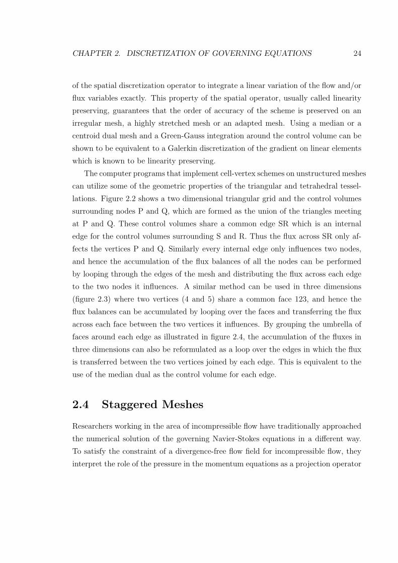
(figure 2.3) where two vertices (4 and 5) share a common face 123, and hence the
flux balances can be accumulated by looping over the faces and transferring the flux
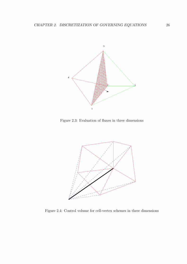
across each face between the two vertices it influences. By grouping the umbrella of
faces around each edge as illustrated in figure 2.4, the accumulation of the fluxes in
three dimensions can also be reformulated as a loop over the edges in which the flux
is transferred between the two vertices joined by each edge. This is equivalent to the
use of the median dual as the control volume for each edge.
2.4 Staggered Meshes
Researchers working in the area of incompressible flow have traditionally approached
the numerical solution of the governing Navier-Stokes equations in a different way.
To satisfy the constraint of a divergence-free flow field for incompressible flow, they
interpret the role of the pressure in the momentum equations as a projection operator

CHAPTER 2. DISCRETIZATION OF GOVERNING EQUATIONS 25
Dirichlet region
Median Dual
Centroid dual
2
4
3
5
6
O
1
Figure 2.1: Dual mesh representation of the control volume
7
6
54
3
21
8R
S
Q
P
910
11
12
Figure 2.2: Nodal formulation of the finite volume scheme
CHAPTER 2. DISCRETIZATION OF GOVERNING EQUATIONS 26
1
2
3
4
5
� � � � � � � � � � � �� � � � � � � � � � � �� � � � � � � � � � � �� � � � � � � � � � � �� � � � � � � � � � � �� � � � � � � � � � � �� � � � � � � � � � � �� � � � � � � � � � � �� � � � � � � � � � � �� � � � � � � � � � � �� � � � � � � � � � � �� � � � � � � � � � � �� � � � � � � � � � � �� � � � � � � � � � � �� � � � � � � � � � � �� � � � � � � � � � � �� � � � � � � � � � � �� � � � � � � � � � � �� � � � � � � � � � � �� � � � � � � � � � � �� � � � � � � � � � � �� � � � � � � � � � � �� � � � � � � � � � � �� � � � � � � � � � � �� � � � � � � � � � � �� � � � � � � � � � � �� � � � � � � � � � � �� � � � � � � � � � � �� � � � � � � � � � � �� � � � � � � � � � � �� � � � � � � � � � � �� � � � � � � � � � � �� � � � � � � � � � � �� � � � � � � � � � � �� � � � � � � � � � � �� � � � � � � � � � � �
� � � � � � � � � � � �� � � � � � � � � � � �� � � � � � � � � � � �� � � � � � � � � � � �� � � � � � � � � � � �� � � � � � � � � � � �� � � � � � � � � � � �� � � � � � � � � � � �� � � � � � � � � � � �� � � � � � � � � � � �� � � � � � � � � � � �� � � � � � � � � � � �� � � � � � � � � � � �� � � � � � � � � � � �� � � � � � � � � � � �� � � � � � � � � � � �� � � � � � � � � � � �� � � � � � � � � � � �� � � � � � � � � � � �� � � � � � � � � � � �� � � � � � � � � � � �� � � � � � � � � � � �� � � � � � � � � � � �� � � � � � � � � � � �� � � � � � � � � � � �� � � � � � � � � � � �� � � � � � � � � � � �� � � � � � � � � � � �� � � � � � � � � � � �� � � � � � � � � � � �� � � � � � � � � � � �� � � � � � � � � � � �� � � � � � � � � � � �� � � � � � � � � � � �� � � � � � � � � � � �� � � � � � � � � � � �
Figure 2.3: Evaluation of fluxes in three dimensions
Figure 2.4: Control volume for cell-vertex schemes in three dimensions

CHAPTER 2. DISCRETIZATION OF GOVERNING EQUATIONS 27
that projects a given velocity field onto a divergence free field. Fractional step or time-
split method are the most popular among these methods. The pressure field that
leads to a divergence free velocity field is typically obtained through the solution of
the Poisson’s equation. This numerical scheme is typically implemented on staggered
meshes (figure 2.5) that store the velocity at the cell faces (u on the j faces and v on
the i faces) and the pressure at the cell center. One of the prime motivation for this
approach is to reduce the decoupling between the velocity and the pressure terms [69]
and hence a decrease in the amount of numerical diffusion required to stabilize the
scheme. While these methods involve no over-head for cartesian meshes, the use
of curvilinear meshes requires storage of both velocity components at each edge to
implement finite volume schemes. Other disadvantages of this approach are that some
of the velocity components are not defined at the boundaries and extension to higher
order is difficult.
Another approach, the use of a half-staggered mesh (figure 2.6) offsets some of
these disadvantages while permitting better coupling between the velocity and pres-
sure fields. In this scheme, the velocity components are stored at the vertices of the
cell and pressure is stored at the cell-center. This allows for the momentum equa-
tions to obtain a pressure distribution around each node and the Poisson equation
for pressure in each cell to be influenced by the velocity at the corners of the cell.
When used in the context of finite volume schemes for hyperbolic equations, the half-
staggered arrangement retains its advantages for curvilinear grids but it is still hard
to implement it on an unstructured grid.
In the next chapter, some results obtained by using a half-staggered arrangement
are presented for two-dimensional flow around airfoils and compared with results from
cell-centered and cell-vertex schemes. Although the estimates of lift and drag from the
different schemes were within acceptable engineering limits, the half-staggered scheme
resulted in pressure distributions that exhibited large errors, especially around the
leading edge. The cause of this discrepancy is not clear and warrants further study.

CHAPTER 2. DISCRETIZATION OF GOVERNING EQUATIONS 28
v
u
p v
vv
u
pv
u
pv
u
pv
u
p
vv
u
pv
u
pv
u
pv
u
p
vv
u
pv
u
pv
u
pv
u
p
u
u
vp
u
u
vp
u
u
p
u
v
Figure 2.5: Staggered arrangement of flow variables
u,v u,v
p
u,v
p
u,v
p
u,v
u,v u,v
p
u,v
p
u,v
p
u,v
u,v u,v
p
u,v
p
u,v
p
u,v
u,v u,v
p
u,v
p
u,v
p
u,v
u,v u,v u,v u,v u,v
p
Figure 2.6: Half-staggered arrangement of flow variables

CHAPTER 2. DISCRETIZATION OF GOVERNING EQUATIONS 29
2.5 Implementation of the Cell-Vertex Scheme
As no immediate benefit was observed from using the staggered arrangement, a cell-
vertex scheme was used in this study for the implementation of the finite volume
scheme on an unstructured tetrahedral mesh. Median-dual mesh cells constructed
from planes bisecting each edge of the mesh are used to accumulate the fluxes at each
node. Boundary conditions are then enforced along the triangular faces that lie on the
boundary to account for the one-sided control volumes for the nodes on the boundary.
The rest of the discussion in this section outlines the details of the implementation of
the spatial discretization operators when used with artificial compressibility methods,
the evaluation of the numerical diffusion terms, and the multigrid algorithm.
2.6 Artificial Diffusion
Numerical diffusion schemes for the solution of transonic and supersonic flows received
wide attention in the late seventies and early eighties. Numerous research efforts dur-
ing this period led to the development of a mathematical framework to add numerical
diffusion to the discretized governing equations with an emphasis to produce shock
profiles that were free of oscillations. This mathematical frame-work can be inher-
ited for incompressible flows that use the artificial compressibility method with some
modifications that limit the amount of numerical diffusion. Local Extremum Dimin-
ishing (LED) schemes that guarantee that new extrema are not generated during the
evolution of the solution have proven to be robust and efficient. These schemes limit
the reconstructed solution and fluxes at cell interfaces by using limiters that can be
constructed from gradient information from a stencil of points around each computa-
tional point. The JST scheme [32] has been widely proven to be a robust frame-work
for numerical diffusion. This scheme can be represented as
dj+ 12
= ε2j+ 1
2∆wj+ 1
2− ε4
j+ 12
(∆wj+ 3
2− 2∆wj+ 1
2+ ∆wj− 1
2
).
When used for problems with embedded supersonic regions, the above scheme
switches to a locally first order scheme to prevent oscillations. For incompressible

CHAPTER 2. DISCRETIZATION OF GOVERNING EQUATIONS 30
flows, the first order term is dropped and the higher order diffusion term is retained to
provide background smoothing. Another choice of numerical diffusion operators based
on the SLIP constructions [36] introduces flux limiters to provide a high resolution
scheme without oscillations. In these schemes, a limited average of the flow variables
is used to construct a flux limiter which is then introduced as an anti-diffusion term
along with a first order diffusive term. A variety of choices exist for the form of the
limited average and the JST scheme can also be rewritten under the class of SLIP
scheme for a particular choice of the limited average.
2.7 Analysis of Artificial Compressibility
In Equation (2.2), Γ is called the artificial compressibility parameter due to the anal-
ogy that may be drawn between the above equations and the equations of motion for a
compressible fluid whose equation of state is given by p = Γ2ρ. Thus, ρ is an artificial
density and Γ may be referred to as an artificial speed of sound. When the tempo-
ral derivatives tend to zero, the set of equations satisfy precisely the incompressible
Euler equations, with the consequence that the correct pressure may be established
using the artificial compressibility formulation. The preconditioning matrix, P , may
be viewed as a device to create a well posed system of hyperbolic equations that are
to be integrated to steady state along lines similar to well established compressible
flow Finite Volume formulations. In addition, the artificial compressibility parameter
may be viewed as a relaxation parameter for the pressure iteration.
The eigen values of the system of equations in equation (2.1) are given by
λ1 = U, λ2 = U, λ3 = U + a, λ4 = U − a,
where,
a2 = U2 + Γ2(ψ2 + η2 + ξ2),
and
U = uψ + vη + wξ.

CHAPTER 2. DISCRETIZATION OF GOVERNING EQUATIONS 31
The terms ψ, η, ξ represent the slopes of the characteristic system of waves, and are
arbitrary and defined.
The choice of Γ is crucial in determining the convergence and stability properties of
the numerical scheme. Typically, the convergence rate and stability of the scheme are
dictated by the slowest system waves and the stability of the scheme by the fastest.
In the limit of large Γ, the difference in wave speeds can be large. Although this
situation would presumably lead to a more accurate solution through the penalty
effect in the pressure equation, very small time steps would be required to ensure
stability. Conversely, for small Γ, the difference in the maximum and minimum
wave speeds may be significantly reduced, but at the expense of accuracy. Thus a
compromise between the extremes is achieved by choosing Γ to be
Γ2 = C(u2 + v2 + w2),
where C is a constant of the order of unity. In regions of high velocity and low
pressure where suction occurs, Γ is large to improve accuracy, and in regions of low
velocity, Γ is correspondingly reduced.
2.8 Time Integration
Under these assumptions on the choice of the preconditioner, P , the application of the
Finite Volume method for a cell-vertex scheme results in a set of ordinary differential
equation for each node of the computational mesh,
d
dt(Viw) + PQi = 0, (2.6)
where Vi is the volume around each node and Qi represents the flux through the faces
of the control volume. To prevent odd-even decoupling at adjacent nodes which may
lead to oscillatory solutions, a dissipation term is added to the flux calculation to
modify the above equation to
d
dt(Viw) + P [Qi −Di] = 0, (2.7)

CHAPTER 2. DISCRETIZATION OF GOVERNING EQUATIONS 32
ord
dt(Viw) +Ri = 0, (2.8)
where Ri is the residual at each node in the computational mesh.
The resulting system is integrated in time using an explicit multistage scheme with
coefficients that maximize the stability region of the time-stepping scheme. To further
accelerate convergence to steady state, local time-stepping and residual averaging
techniques are used. Detailed numerical analysis of the spatial discretization and the
time stepping scheme can be obtained from the following references [32], [36], [67].
2.9 Multigrid Acceleration
Multigrid techniques are widely used to accelerate the convergence of a system of equa-
tions to steady state. A general framework for the development of full-approximation
multigrid methods for non-linear equations can be outlined as follows.
Consider,
Lu = F ,
discretized on a mesh with spacing h as
Lhvh = Fh.
This can be rewritten as
Lh(vh + δvh) = Fh,
where δv represents a correction to the present estimate vh or
Lhδvh +Rh = 0, (2.9)

CHAPTER 2. DISCRETIZATION OF GOVERNING EQUATIONS 33
where Rh is the residual. On the coarse grid, the above equation can be replaced by
L2hδv2h + Ih2hRh = 0, (2.10)
where Ih2h represents the aggregation or restriction operator. The correction to the
present fine grid solution can be represented as
vnewh = vh + I2h
h δvh,
where I2hh represents an interpolation operator. We can add and subtract the following
from equation (2.10)
L2hv2h −F2h = R2h,
to get
L2h(v2h + δv2h)−F2h + Ih2hRh = 0.
This leads to the full approximation scheme (FAS)
L2h(v+2h)−F2h + Ih
2hRh −R2h = 0.
Then
v+h = vh + Ih
2h(v+2h − v2h).
For unstructured grids, the nature of the grids to be used in the multigrid cycle is a
question of ongoing debate. In the present work a series of non-nested meshes are used
for the multigrid cycle and the solution and residual from each mesh are aggregated to
the coarser mesh while interpolating the correction from the coarser to the fine mesh.
Detailed descriptions of the multigrid scheme can be obtained from [37]. Each mesh
of the multigrid cycle was separately generated by a grid generator (MESHPLANE).
A detailed description of the multigrid scheme can be obtained from [37]. The
initial solution from a particular mesh is advanced in pseudo-time to obtain new

CHAPTER 2. DISCRETIZATION OF GOVERNING EQUATIONS 34
n1
n2
n3
a1
a2
a3
p
Figure 2.7: Interpolation coefficients for use in the multigrid cycle
estimates of the flow variables. On transfer to the next level of the multigrid, the
solution for the coarse grid mesh points are interpolated from the four nodes of the
fine mesh tetrahedron that contains this node. Further, the accumulated residual
at each fine mesh point is distributed to each node of the tetrahedron in the coarse
mesh that that encloses the fine mesh node. The interpolating factors for each node
are computed from weights which are based on the volume included by a given node
and opposite face of the tetrahedron (figure 2.7). This reduces to a second order
interpolation scheme on equilateral tetrahedra and has been found to be sufficient
for the present calculations. The solution that is transferred to the coarse mesh and
the estimate of the residuals from the fine mesh are used by the coarse mesh to
remove/convect error terms in the residuals that can be most efficiently tackled by
the coarse mesh. Further levels in the multigrid cycle involve the same operations
are before, thereby using grids that are coarser and coarser to convect the error
terms out of the computational domain faster. The ascend of the multigrid cycle
estimates a correction from each grid which is then interpolated to the fine mesh
points (figure 2.8). The corrections from the coarser mesh are transferred using
similar interpolating factors as for the aggregation operations. Multigrid cycles which
progress in the shape of a W have been known to provide faster convergence to steady
state than the V cycle.

CHAPTER 2. DISCRETIZATION OF GOVERNING EQUATIONS 35
fine grid nodes
coarse grid nodes
� � �� � �� � �� � �
� � �� � �� � �� � �
Figure 2.8: Transfer of solution, residuals and corrections between the fine and coarsemesh
2.10 Parallel Implementation
To make use of the availability of parallel computing facilities, the numerical scheme
and the computational methodology described in the previous sections were imple-
mented in a computer program that used the Message Passing Interface (MPI) stan-
dard to enable parallel computations. The rest of the this section describes the parallel
implementation of the flow solver on an unstructured tetrahedral grid.
2.10.1 Domain Decomposition, Load Balancing
Computational tests performed by Jameson [38] showed that the use of a domain
decomposition algorithm reduced the stride in the numbering of the vertices at each
edge of the mesh resulting in a reduction of computational times by a factor of three.
The domain decomposition algorithms used in this study was a modified form of
the coordinate bisection method that led to sub-domains with approximately equal
number of computational nodes (figure 2.9).
To construct a partition of the computational mesh for parallel implementation,
the above mentioned domain decomposition method was reused and the resulting
sub-domains were distributed among the available processors while balancing the

CHAPTER 2. DISCRETIZATION OF GOVERNING EQUATIONS 36
9
8
7
6
54
3
10y
x
16
15
11
12
1314
21
Figure 2.9: Domain decomposition of a rectangular region using a bisection method
load among them. This methodology worked well for the problems in this study.
Extensions to viscous flows will require more sophisticated graph partitioning algo-
rithms that distribute the computational nodes equally to all the processors while
minimizing the number of edges that are shared between the processors.
A set of sub-domains which is produced by the above partitioning method is
distributed among the set of available processors by considering a combination of
computational complexity for each domain along with the cost of communication
across processor boundaries. No further attempt was made to redistribute the points
within each sub-domain to minimize the cost of communication arising from edges
that are shared across processor boundaries. Once the partitions are distributed
among the processors, data structures that allow for the exchange of information
along processor boundaries are constructed. As the flow solver uses an edge-based
data structure to accumulate the fluxes at each vertex, the edges surrounding the
nodes that lie within a partition are accumulated. If an edge connects a point across
processor boundaries, this edge is duplicated in the two processors and ‘halo’ nodes
are constructed for both processors. This idea is illustrated further in figure 2.10.

CHAPTER 2. DISCRETIZATION OF GOVERNING EQUATIONS 37
inter-processor boundary
edges that are shared between processors
Figure 2.10: Halo nodes and the distribution of edges along processor boundaries
2 4 6 8 10 12 14 162
4
6
8
10
12
14
16
Number of Processors
Spe
edU
p
Actual SpeedUpIdeal SpeedUp
Figure 2.11: Speedup from the parallel implementation
CHAPTER 2. DISCRETIZATION OF GOVERNING EQUATIONS 38
2.10.2 Parallel implementation of the multigrid algorithm
The use of multigridding techniques for flow analysis necessitates the need to ex-
change information between a fine and coarse grid point and vice-versa. While the
residuals from the fine grid points need to be accumulated at the coarse grid points,
the corrections from the coarse grid points need to be transferred back to the fine grid
points. In this study a non-nested approach to multigridding has been used and the
sequence of meshes are repeatedly generated from a mesh generator. Hence, efficient
methods have to be used to generate the interpolation coefficients by identifying the
cell in the fine grid or coarse grid that contains a given point.
A ‘naive’ implementation of the point search algorithm results in an algorithm
with complexity kO(n2), where n is the number of nodes in the computational mesh.
This is clearly not acceptable for computational meshes where the number of nodes
are typically of the order of a few hundred thousand. Octree-based search algorithms
are known to be efficient for such problems. The computational complexity of an
octree based search algorithm is O(log(n)). Due to the superior performance of the
octree-based search routine, this method was implemented to perform point searches.
To implement the octree searches, a tree data structure to hold the octants and
its extents is first determined for each mesh. Each octant is allowed to hold a certain
number of points. Once an octant contains more than an user specified set of points,
then the octant is sub-divided to create 8 new octants. Using this data structure, a
given point is identified within an octant and the node closest to a point in this octant
is determined. The cells that meet this node are checked to see if they contain the
search point. The efficiency of the octree method lies in its ability to quickly localize
the search process to a small region of the computational mesh.
The octree based search routine has been found to be very useful for the imple-
mentation of the non-nested multigrid methods as the major cost during the pre-
processing step is associated with the point search routines to compute the inter-
polation coefficients between successive meshes. Using the octree data structure,
interpolation coefficients between a fine grid node and the next coarser mesh in the
multigrid cycle is constructed in a pre-processing step. Further, to reduce the cost
communication across processors during each multigrid cycle, sub-domains on the

CHAPTER 2. DISCRETIZATION OF GOVERNING EQUATIONS 39
coarser grids are constructed and distributed to the processors so as to conform to
the division and distribution of the fine mesh. Typical computational times for the
building of the octree and the subsequent point search algorithms are in the range of
a few minutes for a mesh sequence containing a million nodes.
An alternate implementation of the octree based point search algorithm was also
implemented and found to very efficient. This method uses the sub-domains created
by the domain decomposition algorithm to identify the domain that contains the given
search point. Then the cells in that sub-domain are queried to see if they contain the
given point. As the sub-domains are already created for load balancing, this approach
eliminates the need to construct the octree data structure. Hence the computational
time for this method was comparable to that of the octree based searches and it is
exteremely trivial to implement.
2.10.3 Speedup of the Parallel Implementation
Several test cases were used to test the implementation of the parallel flow solver.
Figure 2.11 shows the typical speed-up observed for these cases. The meshes in
these studies typically contained about half a million nodes in the fine mesh. Due
to the reduction in the stride of the node numbering for the edges in each sub-
domain, more than linear speed-up was observed for 4 and 8 processor runs. However,
as more processors we employed the domain decomposition algorithms resulted in
partitions that were sub-optimal leading to increased communication cost among the
processors thereby resulting in less than linear speed-up. Hence, there is a definite
need to improve the domain decomposition algorithm for larger problems. Most of
the calculations for this study were performed using 8 processors.
2.11 Governing equations and analysis of the struc-
tural model
In order to determine the static or dynamic displacements of a structure under the
action of external and/or body forces the elasticity equations need to solved. For a
CHAPTER 2. DISCRETIZATION OF GOVERNING EQUATIONS 40
general three dimensional structure these equations involve fifteen unknowns (three
displacements, six stresses and six strains) and hence a set of fifteen equations are used
to describe the state of the structure. Under varying assumptions of the properties of
the model, these equations can be simplified and the principle of virtual work along
with the ‘Unit Displacement Theorem’ can be used to lay the foundation for the finite
element method which has become the choice for most structural analysis problems.
For a general three dimensional structure the components of strain can be related
to the displacement field through he following equations.
εii =∂ui
∂xi
, εji = εij =∂ui
∂xj
.
Now, the strains can be related to the stresses and if the material is assumed
to be isotropic, the stress-strain relations are related through the Young’s modulus
and the Poisson’s ratio. Using the equilibrium equations, the elasticity equations in
three dimensions can be formulated. To arrive at a set of discrete set of equations,
a Galerkin formulation can be used to reduce the strong form of the problem into
a weak formulation. This involves multiplying the equilibrium equations by a shape
function and integrating over the domain of interest and reducing the integral using
integration-by-parts. To numerically solve this set of equations, the domain of interest
is broken into finite elements which are typically triangles or quadrilaterals. Assuming
a particular form of the shape function (linear for Galerkin formulations) along with
a basis to represent the displacement field leads to a set of linear equations relating
the unknown displacement field and the external forces. This set of linear equations
usually assumes the form
[k]x = F,
where k is the global stiffness matrix, x is the displacement vector under investigation
and F is the external force at the nodes at which the displacement is sought. The form
of the stiffness matrix is dependent on the nature and type of elements used to repre-
sent the body. While triangular elements allow for ease of representation of arbitrary
geometries, they usually turn out to be stiffer than quadrilateral elements. Higher

CHAPTER 2. DISCRETIZATION OF GOVERNING EQUATIONS 41
order approximations for the variation of the displacements and strains within in each
element can also be used to capture sharply varying changes in the displacement field.
Most commercial finite element packages provide means to choose elements and the
basis functions to approximate the displacement field. Triangular or quadrilateral ele-
ments with a linear basis are typically chosen for most problems. Further, procedures
to assemble the stiffness matrix and solve the resulting system of equations are also
provided, thereby allowing the structural analysis package to be used as black-box
that dumps out the displacements for a given loading.
2.11.1 Structural Model of the Sail
The sail cloth was discretized into finite elements (after neglecting the presence of
batten pockets) with a set of quadrilateral membrane elements with four nodes. These
elements withstand all external forces through tension and are essentially incapable
of resisting bending moments. The translational and rotational degrees of freedom
along the foot of the main sail was suppressed. Along the mast, the translational
degrees of freedom was inhibited while allowing for rotational motion. For the head
sail, the point of attachment of the foot to the rig was constrained. The leech of
the main and head sail were allowed to move freely to induce a geometric twist
due to the aerodynamic loading. The mast was assumed to be rigid during the
structural and aeroelastic calculations. The presence of battens and tension cables
and other structural elements of the sail rig was neglected from this analysis. The
linear system of equations relating the displacements to the force field was advanced to
a steady state by a iterative process that incrementally added the load while obtaining
a converged displacement field for each step. This non-linear model to predict the
deflected shape of the sail was included in anticipation of large deflections of the sail
geometry. Wrinkling of the structure, which is an important consideration especially
around the leading edge (luff) and at the sail tip, is not anticipated by this model
but the use of methodology to large deformations allows for wrinkling models to be
included at a later stage.
For Americas Cup sails it is important to account for the yarn layout as it gives rise
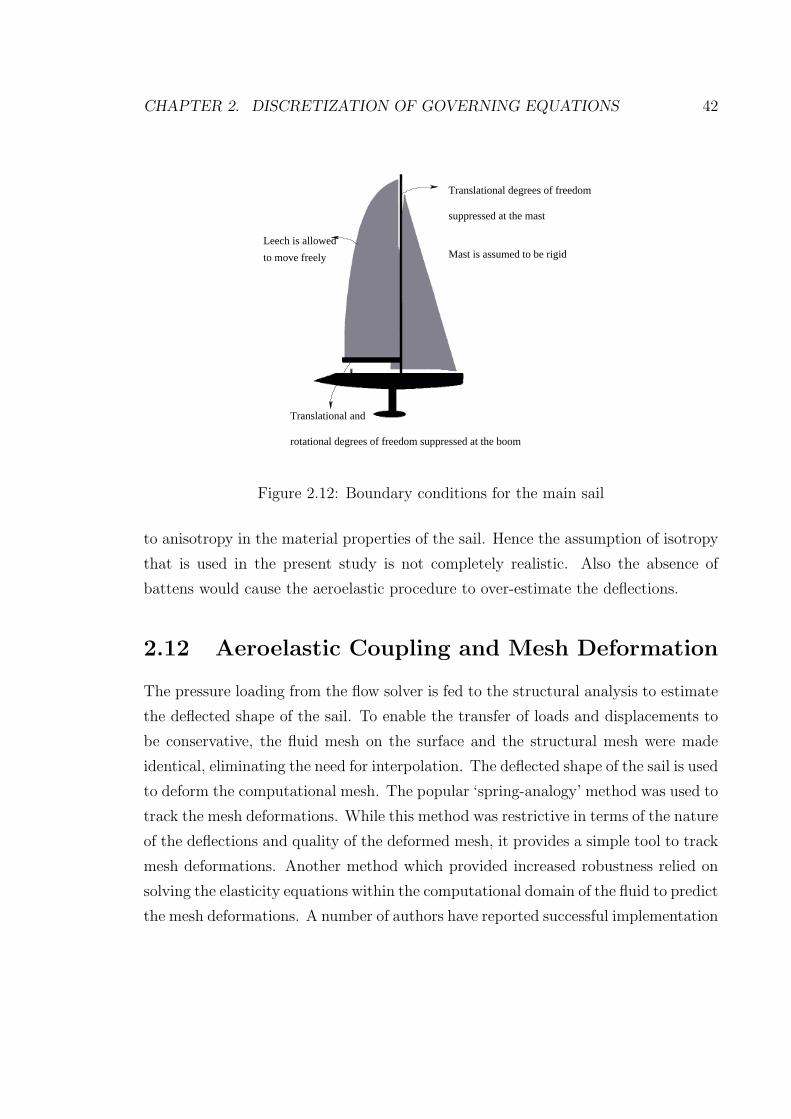
CHAPTER 2. DISCRETIZATION OF GOVERNING EQUATIONS 42
Leech is allowed
to move freely
Translational degrees of freedom
suppressed at the mast
Mast is assumed to be rigid
Translational and
rotational degrees of freedom suppressed at the boom
Figure 2.12: Boundary conditions for the main sail
to anisotropy in the material properties of the sail. Hence the assumption of isotropy
that is used in the present study is not completely realistic. Also the absence of
battens would cause the aeroelastic procedure to over-estimate the deflections.
2.12 Aeroelastic Coupling and Mesh Deformation
The pressure loading from the flow solver is fed to the structural analysis to estimate
the deflected shape of the sail. To enable the transfer of loads and displacements to
be conservative, the fluid mesh on the surface and the structural mesh were made
identical, eliminating the need for interpolation. The deflected shape of the sail is used
to deform the computational mesh. The popular ‘spring-analogy’ method was used to
track the mesh deformations. While this method was restrictive in terms of the nature
of the deflections and quality of the deformed mesh, it provides a simple tool to track
mesh deformations. Another method which provided increased robustness relied on
solving the elasticity equations within the computational domain of the fluid to predict
the mesh deformations. A number of authors have reported successful implementation

CHAPTER 2. DISCRETIZATION OF GOVERNING EQUATIONS 43
the stayfreedom supressed alongTranslational degrees of
All degrees of freedom suppressed
mast
clew foot
leech
luff
head
stay
Figure 2.13: Boundary conditions for the head sail
of this method for aeroelastic problems, adaptive refinement techniques and in surface
propagation problems. The deformed mesh is then used to compute a new pressure
loading for the sail. This iterative process offers no guarantee of convergence but
typically predicts the deflected shape to reasonable accuracy in a few steps (typically
4-7 for sail geometries).
Mesh deformation techniques in aeroelastic computations are typically posed as
problems in structural mechanics. The most popular ‘spring-analogy’ method de-
termines the new position of the nodes of the computational mesh by imposing the
boundary displacements as initial conditions and solves for the equations of static
equilibrium for each node. To model the computational mesh as a structural mem-
ber, a stiffness is associated with each edge of the mesh. This stiffness is typically
inversely proportional to the length of the edge. This allows for control of points
which are bunched close to each other.
The spring method can be mathematically conceptualized as solving the following
equation

CHAPTER 2. DISCRETIZATION OF GOVERNING EQUATIONS 44
∂∆xi
∂t+
N∑j=1
Kij(∆xi −∆xj) = 0,
where the Kij is the stiffness of the edge connecting node i to node j and its value
is inversely proportional to the length of this edge, ∆xi is the displacement of node
i and ∆xj is the displacement of node j, the opposite end of the edge. The position
of static equilibrium of the mesh is computed using a Jacobi iteration with known
initial values for the surface displacements.
The spring method has been known to either degrade the quality of the mesh or
produce ‘inverted’ meshes when the boundary deformations are not small. To over-
come some of these failings, some researchers have used the spring-analogy method
in conjunction with edge-swapping routines to ensure that the quality of the mesh
does not degrade during the computations.
A more robust mesh movement scheme that overcomes this limitation can be
constructed by modeling the domain as an elastic solid and solving the equilibrium
equations for the stress field. In terms of the displacement vector u the strain tensor
can be written as
εij =1
2
(∂ui
∂xj
+∂uj
∂xi
), i, j = 1, 2, 3.
For an isotropically elastic solid the stress tensor is defined as
σij = λεkkδij + 2µεij,
where λ and µ are the Lame constants, δij is the Kroneckar delta and the summation
convention has been invoked. If there is no distributed body force the stress field
satisfies the equation∂σij
∂xij
= 0.
Dividing by the shear modulus µ leads to an equation that depends only on the
parameter λ/µ. Alternatively, one can introduce Poisson’s ratio ν λ2(λ+µ)
and consider
this to be the user defined parameter. It is again possible to increase the rigidity

CHAPTER 2. DISCRETIZATION OF GOVERNING EQUATIONS 45
of the mesh in regions of small element size and/or bad element aspect ratio, by
modifying the coefficients λ and µ.
Further research needs to be performed to identify the optimal mesh deformation
technique for aeroelastic calculations of sail geometries.

Chapter 3
Analysis of Sail Configurations
This chapter presents the results obtained from using the flow solver and the aeroe-
lastic package on sail geometries. The incompressible flow solver is used to study
the effect of the mast, apparent wind angle and heel on the aerodynamic perfor-
mance of the sail configurations. Aeroelastic simulations were performed to study the
importance of sail elasticity on the pressure distribution over the sails.
The behavior of the finite volume scheme for the compressible flow equations
in the low Mach number regime and at high angles of attack is analyzed first. As
representative examples, multi-element airfoil configurations and three dimensional
sail computations are performed to test the robustness and accuracy of the numerical
scheme. After verifying that these simulations provide good engineering estimates, the
artificial compressibility correction is next introduced, and it is then used to study
airfoils in two dimensional flow and single and multi-element sail configurations in
three dimensional flow. Finally the flow solver is coupled to a structural model to
obtain steady deflected shapes of the sail configurations.
46
CHAPTER 3. ANALYSIS OF SAIL CONFIGURATIONS 47
3.1 Low Mach number, high angle of attack simu-
lations with a compressible flow solver
3.1.1 Multi-Element airfoils
The operational conditions of a high lift system provide an aerodynamic analogy to
the thrust producing mechanism of sails in close-hauled conditions. In order to vali-
date the numerical scheme, a three element airfoil configuration was analyzed using a
two dimensional version of the finite volume scheme on unstructured grids. The grids
were generated using a mesh generator which uses Delaunay criterion to triangulate a
set of points. The grid shown in figure 3.1 contains 20,000 triangles in the fine mesh.
The finite volume scheme is implemented on a dual of the underlying Delaunay trian-
gulated mesh with modified Runge-Kutta time stepping schemes, residual averaging,
the JST scheme for the numerical diffusion and multigrid techniques to get to steady
state. The pressure distribution over the three elements is shown in figure 3.1. The
distribution of entropy on the surface is shown using normals in figure 3.1. As ex-
pected, the trailing edge of the slat, main and the flap show larger entropy than
the remainder of the section. The overall pressure distribution follows engineering
intuition and compares well with a structured grid flow solver, FLO103 [39]. The
suction peaks around the leading edge of the main, flap and the slat are critical to
the production of high lift and are recovered well by the numerical scheme. Quantities
of engineering interest (lift and drag) typically converge in under hundred iterations.
The results of the tests with this configuration confirmed the robustness of the nu-
merical scheme for low Mach number, high angle of attack problems on unstructured
grids.
3.1.2 Sail simulations
Low mach number compressible flow simulations over a sail geometry were performed
next. Simulations were performed for Mach numbers up to 0.1 and angles of attack
ranging from 8 to 20 degrees. The numerical scheme was robust within this range of
flow conditions. However, further reduction in the Mach number required increased
CHAPTER 3. ANALYSIS OF SAIL CONFIGURATIONS 48
levels of numerical diffusion to arrive at converged solutions. Figure 3.2 shows the Cp
distribution at two sections along the sail and also shows typical convergence rates for
this geometry. The presence of the mast induces a sharp leading edge suction peak
and a strong pressure gradient which could have adverse effects on the boundary
layer development on the upper surface of the sail. The oscillations near the trailing
edge are due to a combination of problems. The Kutta condition is not strongly
enforced in these flow simulations but is usually recovered due to the concentration
of computational points around the trailing edge. Further, as the thickness of the
sail geometry is rather small, most mesh generation programs result in a mesh with
poor quality along the trailing edge. However, it must be pointed out that the use of
artificial compressibility methods greatly reduces the magnitude of these oscillations
(see results in the subsequent sections). While the wind speeds for these calculations
are beyond the reach of most racing boats, this test re-enforces belief in the underlying
numerical scheme for sail geometries at high angles of attack.
3.2 Effect of Numerical Discretization and diffu-
sion on artificial compressibility methods
As discussed in the previous chapter, it is possible to implement the numerical proce-
dure that integrates the governing equations using different arrangements of the flow
variables. In order to study the behavior of three different arrangements (cell-vertex,
cell-centered and the half-staggered scheme) an airfoil in incompressible flow was an-
alyzed. All three schemes used the same numerical scheme, namely the finite volume
scheme, artificial compressibility corrections, second order construction of the convec-
tive fluxes, SLIP construction for the numerical diffusion and Runge-Kutta multistage
time integration schemes. For the half-staggered arrangement, at the solid wall, flow
tangency and pressure boundary conditions were applied. All three approaches used
a ‘vortex-corrected’ far-field boundary condition. To compare the pressure distribu-
tions obtained from these simulations, potential flow solutions were obtained using
FLO1 (figure 3.3). The deviation of the computed solution on the airfoil surface from
CHAPTER 3. ANALYSIS OF SAIL CONFIGURATIONS 49
the Bernoulli’s equation was recorded for each test and used as a basis for comparing
the three flow solutions. The pressure distribution for the cell-centered, cell-vertex
and the half-staggered arrangement are shown in figures 3.4, 3.5, 3.6 respectively. The
error in satisfying the Bernoulli’s equation is shown in figures 3.7, 3.8, 3.9, 3.10. It can
be seen from these plots that the cell-centered scheme has the least error, followed
by the cell-vertex scheme. The half-staggered arrangement seems to display large
errors near the leading edge stagnation point, a feature that is less prominent for the
cell-vertex and the cell-centered schemes. Further research needs to be performed
to study the cause of this behavior as it seems to contradict the popular belief that
half-staggered arrangements lead to less decoupling between the pressure and veloc-
ity components thereby yielding more accurate solutions. The cell-vertex scheme has
advantages over the cell-centered scheme when used with three dimensional unstruc-
tured grids and as the difference in the accuracy of the solution was not appreciable,
cell-vertex schemes were used for the subsequent problems in this study.
3.3 Validation of the parallel implementation
Parallel implementation of the flow solver was tested against solutions from the single
processor version of the solver and previously existing solutions from other computa-
tional programs (FLO87).
A variety of geometries ranging from wing to complete aircraft configurations were
analyzed with the compressible version of this parallel program. The meshes were
generated using MESHPLANE, an unstructured grid generator which uses the Delau-
nay criterion to connect points in the field to form tetrahedra. Single grid calculations
typically take 300 to 400 flow cycles to reach a converged solution on a mesh with
350000 nodes. Coarser levels of the multigrid cycle were regenerated with MESH-
PLANE by typically halving the number of nodes in the mesh. The triangulation of
the surface was retained in the coarser meshes to recover the geometry but it was
found to be not so critical for some of the problems. Typically, 3 levels of multigrid
were used for the aircraft configurations and converged solutions can be obtained in
about 60-70 multigrid cycles. The results for these simulations compare well with

CHAPTER 3. ANALYSIS OF SAIL CONFIGURATIONS 50
the results from a single processor version of the program thereby establishing the
robustness of the parallel implementation of the flow solver.
3.4 Single and multi-element sail computations with
artificial compressibility methods
Having identified a suitable numerical discretization scheme for the artificial com-
pressibility method and validated the parallel implementation of the flow solver, the
flow around sail configurations was analyzed to obtain estimates of lift, drag and
heeling moment along with detailed pressure distributions at various heights of the
sail. The aim of this study was to characterize the performance of the sail for a va-
riety of conditions, thereby allowing the designer to judge the quality of the design.
Simulations were performed with the main sail alone and for a head and main sail
combination.
The computational domain typically extended 10 body lengths in all three co-
ordinate directions. For computations with the main sail alone, the foot of the sail
coincided with the symmetry plane and for computations with the head and the main
sail, the symmetry plane was off-set from the sail geometries. Twisted inflow condi-
tions were prescribed at the inlet to simulate the twisted boundary layer profile of
the incoming air-stream. The meshes were generated with MESHPLANE. Typically,
around 2 million cells were used for the single sail computations and around 4 million
cells were used for the head and main sail combination. Meshes for the coarser levels
in the multigrid cycle were regenerated using MESHPLANE and typically the number
of cells/nodes in the mesh was halved for each coarser mesh. For all the simulations a
W cycle was used for the multigrid calculations. 75-100 multigrid cycles were needed
to obtain converged estimates of the lift and the drag.
3.4.1 Characteristics of the main sail
This section discusses the performance of the main sail. Figure 3.12 shows the pressure
distribution at 3 sections along the height of the sail. The pressure distribution near

CHAPTER 3. ANALYSIS OF SAIL CONFIGURATIONS 51
the foot exhibits a sharp peak around the leading edge of the upper surface. However,
due to the absence of a gap between the foot of the sail and the free-surface, the results
along the lower sections will at best be qualitative. Typically, these sections do not
produce much lift due to the tendency of the flow to equalize the pressure on the
upper and lower surface by using the gap between the foot of the sail and the deck.
Along the mid and upper sections of the sail, the flow enters the sail at the optimum
angle suggesting that the twist of these sections have been aligned with the incoming
flow. The flow is smooth through the remainder of the sail planform with a mild
deviation near the trailing edge of each section. As the current numerical scheme
does not explicitly impose the Kutta-condition but hopes to recover it through the
distribution of points in the field and the geometry, the flow does not pass smoothly
over the trailing edge. Further, the presence of a blunt trailing edge attenuates the
problem while also clouding the physics of an inviscid flow around a sharp trailing
edge. Figure 3.13 shows the distribution of the span-wise force coefficients. The sail
sections operate at roughly the same lift coefficient from the foot to the tip. While this
is desirable in light wind conditions when the heeling moment produced by the sail
can be stabilized by the allowable ballast weight, it is not so desirable in heavy wind
conditions. As the sails sections have been twisted to account for the upwash created
by the bound vortex, the occurrence of tip induced stall has been reduced allowing the
sail sections to stall at the same time. On the flip side, the uniform loading produced
by the main sail results in a large tip vortex and hence an associated increase in drag.
The forces generated by the main sail under a range of close-hauled incident wind
angles is shown in figure 3.14. This figure exhibits the typical behavior of sails sailing
towards the wind. Maximum lift coefficients of around 1.6 at 22.5 degrees of wind
incidence with an associated L/D of 8.83 are typical of the sails used in Americas
Cup.
To study the effect of the mast on these simulations, the above experiments were
repeated with a mast. The mast was assumed to have an elliptic cross-section and
was oriented with the tangent to luff at each section to minimize the influence of
the mast. The major axis of the mast was 8 inches long and the minor axis was 1
inch wide. Figure 3.15 shows the effect of the mast with increasing angle of attack.

CHAPTER 3. ANALYSIS OF SAIL CONFIGURATIONS 52
Until about 10 degrees the effect of the mast is not very pronounced. At higher
angles of attack, the presence of the mast induces higher lift and drag coefficients.
Experimental studies by Milgram [12] shows that the presence of the mast could
increase the form and pressure drag of the sail to match the induced drag depending
on its shape and orientation to the incoming air-stream. The interaction of the mast
with the pressure distribution on the sail is strongly influenced by viscous effects
originating from the development of the boundary layer in adverse pressure gradients
and hence the current study is only able to a qualitative picture of the flow physics.
The performance of the sail usually degrades as it heels mainly due to the inter-
action of the sail with the free surface of the sea and the change in the sail trim to
the incoming air-stream. Due to restrictions on the weight of the ballast, most high
performance yachts sail upwind at a heel angle while paying the associated loss in lift
and drag. Numerical experiments were performed to study the effect of the heel with
an aim to identify the maximum allowable heel angle. Figure 3.16 shows the lift and
drag at various apparent wind angles for two different heel angles. This figure shows
that the reduction in lift and increase in drag is more pronounced at higher incidence
angles and can be as high as 15 %.
3.4.2 Characteristics of the Head and Main sail combination
A head and main sail combination [13] was analyzed next. The planform and section
characteristics of the main and head sail are shown in figures 3.17 and 3.18. It can
be seen that the head sail has a triangular planform while the main has an elliptic
chord distribution. The twist distribution of the head and the main sail increases
from the foot to offset the upwash created by the other sail. Further, the maximum
camber and it position also increases from the foot to the head of the sail. Sails are
usually designed to have increasing camber towards the head to provide for favorable
pressure gradients that would delay the onset of separation or reduce the increase in
drag from a turbulent/separated boundary layer. This configuration was tested at a
heel angle of 25 degrees with the apparent wind angle of 19 degrees at a height of 10
meters along the sail. The onset flow was twisted to result in a parabolic distribution

CHAPTER 3. ANALYSIS OF SAIL CONFIGURATIONS 53
of the velocity magnitudes.
The span-wise loading of the head and the main sail are shown in figure 3.21
and 3.22. The head sail displays a desirable pressure loading where the lift gradually
tapers towards the tip and has an elliptic distribution. This results in a weaker
trailing vortex at the tip and hence reduced drag. Both the lift and the drag have
oscillations near the foot possibly due to the gap between the foot and the symmetry
plane. The loading of the main sail displays a gradual increase towards the tip which
is an undesirable feature. This feature become more prominent above the head sail
showing that favorable pressure gradients induced by the head sail have significant
influence on the pressure profiles of the main sail sections. The presence of this region
on the main sail with large suction peaks could be detrimental to the development of
the boundary layer and possible separation. Due to the absence of a viscous model
in the present analysis it is difficult to make quantitative estimates of the loss in lift
by the main sail. One of the potential applications of a shape optimization design
procedure would be to determine the optimal shape of the main sail that either
eliminates separation or delays its onset.
The pressure distribution around the leading edge of the main sail shows the
influence of the jib. The leading edge peak has been suppressed providing a more
favorable pressure gradient leading to a reduced probability of separation and stall.
The favorable influence of the head sail allows the main sail to be set at a higher
angle of attack without flow separation and stall. The pressure distribution on the
head sail shows some undesirable features. Along the leading edge of the mid and
upper sections, the flow enters at an angle different from the optimum. This leads to
a small region of ‘inverted’ pressure profiles which could be offset by altering the twist
or camber distribution of these sections. However, due to the upwash created by the
bound vortex around the main sail, the task of identifying the optimum head sail twist
and camber is not straight-forward. Further, these simulations were performed on an
undeformed head and main sail combination and as discussed in the next section,
the aeroelastic effects cause the twist and camber distribution to be altered thereby
eliminating some of the undesirable pressure profiles on the head sail.
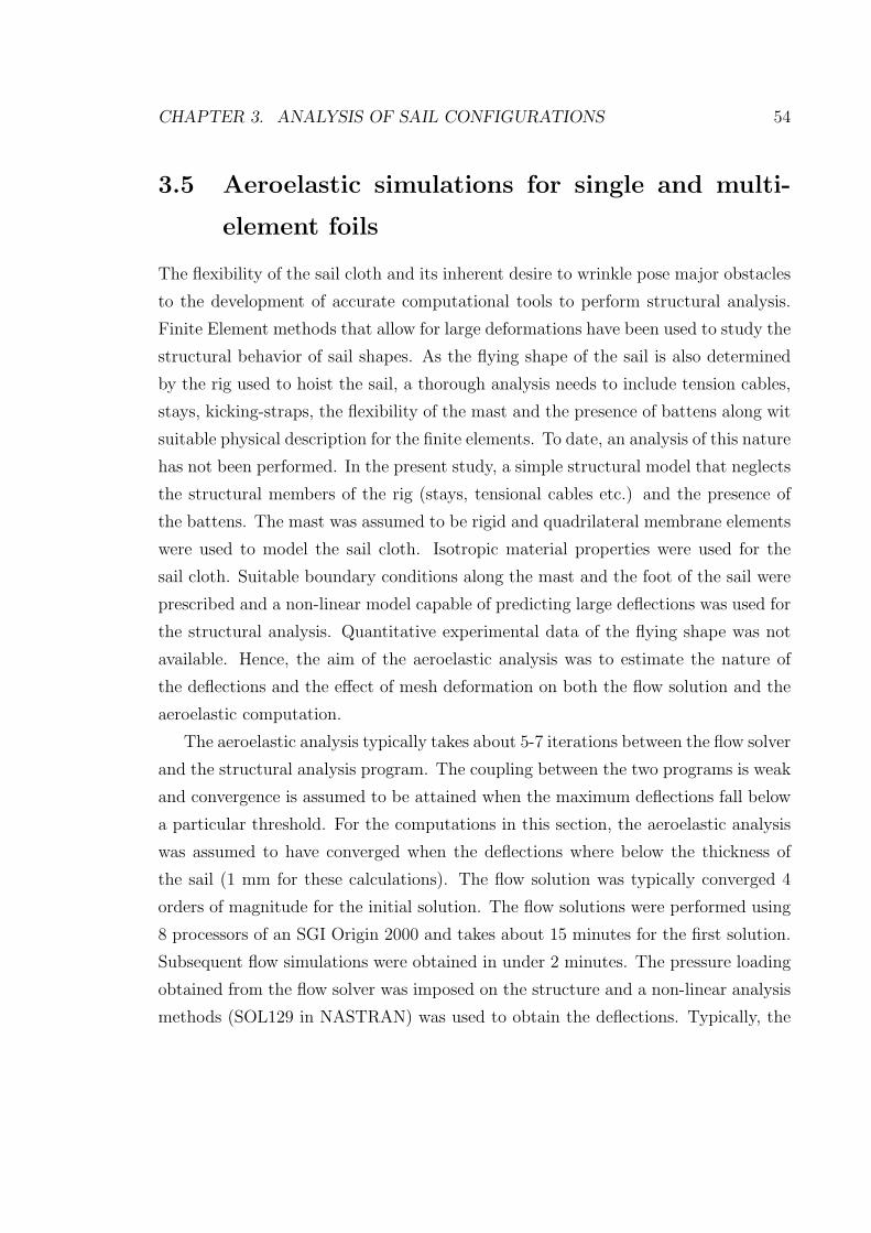
CHAPTER 3. ANALYSIS OF SAIL CONFIGURATIONS 54
3.5 Aeroelastic simulations for single and multi-
element foils
The flexibility of the sail cloth and its inherent desire to wrinkle pose major obstacles
to the development of accurate computational tools to perform structural analysis.
Finite Element methods that allow for large deformations have been used to study the
structural behavior of sail shapes. As the flying shape of the sail is also determined
by the rig used to hoist the sail, a thorough analysis needs to include tension cables,
stays, kicking-straps, the flexibility of the mast and the presence of battens along wit
suitable physical description for the finite elements. To date, an analysis of this nature
has not been performed. In the present study, a simple structural model that neglects
the structural members of the rig (stays, tensional cables etc.) and the presence of
the battens. The mast was assumed to be rigid and quadrilateral membrane elements
were used to model the sail cloth. Isotropic material properties were used for the
sail cloth. Suitable boundary conditions along the mast and the foot of the sail were
prescribed and a non-linear model capable of predicting large deflections was used for
the structural analysis. Quantitative experimental data of the flying shape was not
available. Hence, the aim of the aeroelastic analysis was to estimate the nature of
the deflections and the effect of mesh deformation on both the flow solution and the
aeroelastic computation.
The aeroelastic analysis typically takes about 5-7 iterations between the flow solver
and the structural analysis program. The coupling between the two programs is weak
and convergence is assumed to be attained when the maximum deflections fall below
a particular threshold. For the computations in this section, the aeroelastic analysis
was assumed to have converged when the deflections where below the thickness of
the sail (1 mm for these calculations). The flow solution was typically converged 4
orders of magnitude for the initial solution. The flow solutions were performed using
8 processors of an SGI Origin 2000 and takes about 15 minutes for the first solution.
Subsequent flow simulations were obtained in under 2 minutes. The pressure loading
obtained from the flow solver was imposed on the structure and a non-linear analysis
methods (SOL129 in NASTRAN) was used to obtain the deflections. Typically, the

CHAPTER 3. ANALYSIS OF SAIL CONFIGURATIONS 55
pressure loading was broken into 25 incremental steps. The structural simulations
were performed on a single processor and typically take about 2-3 minutes. The
spring method was used to deform the CFD mesh. While this method is not entirely
desirable for large deformations that are typically encountered with sail geometries,
it is extremely trivial to implement and usually takes about 10-20 seconds when
computed with multiple processors (typically 8). During the aeroelastic iterations it
was sometimes observed that the deformed mesh degrades in quality which adversely
affects the flow solution and hence the overall aeroelastic procedure. This difficulty
was reduced to some extent by breaking the deflections into incremental steps and
deforming the mesh after each step. Alternately, the mesh generation program could
be used to regenerate the mesh but this would entail transferring the flow solution
from the previous iterations using interpolation coefficients. This approach was not
explored for the results presented here.
The deflected shape of the head and the main sail are shown in figures 3.24
and 3.25. It can be seen from these plots that the lower sections of the head and
the main sail do not undergo appreciable deformation. The largest deflections occur
in the mid-sections of the main sail. Due to the absence of battens in the structural
model, it is believed that the deflections predicted by the aeroelastic procedure would
be greater than those observed on the true flying shape.
As the point of attachment of the main sail to the mast and the leading edge of
the head sail was not allowed to move, the pressure loading altered the twist of the
sail geometry. This had a favorable influence on the pressure distribution, especially
on the head sail (figures 3.26 and 3.27). The pressure distribution over the head
and sail after the aeroelastic simulation highlights the need to perform aeroelastic
analysis for sail geometries. While the lift and the drag of the deformed shape is not
significantly different from the undeformed shape, the pressure distribution over the
sail sections shows that the twist and the camber distribution can be altered by the
pressure loading that can potentially alter the flow around the head and the main
sail.

CHAPTER 3. ANALYSIS OF SAIL CONFIGURATIONS 56
AGARD-AR-303 MACH 0.200 ALPHA 8.230
CL 3.5407 CD 0.0483 CM -0.6802
NODES 11158 NCYC 2500 RES0.530E-04
3.
00
2.00
1.
00
0.00
-1.
00 -
2.00
-3.
00 -
4.00
-5.
00 -
6.00
-7.
00
Cp +
+
+++++++++++++++++++++++++++++++++++++++++++++++++++++++++++++++++++++++++++++++++
+++++++++++
+++++++++++++++++++++++++++++++++++++++++++++++++++++++++
+
+
+
++++++++++++++++++++++++++++++++++++++++++++++++++++++++++++++++++++++++++++++++++++++++++++++++++++++
++++++++++++++++
++++++++++++
++++++++++++++++++++++++++++++++++++++++++++++++++++++++++++++++++++++++++++++++++++++++++++++++++++++++++++++
++
+
++
+
3.
00
2.00
1.
00
0.00
-1.
00 -
2.00
-3.
00 -
4.00
-5.
00 -
6.00
-7.
00
Cp
+
+
+++++++++++++++++++++++++++++++++++++++++++++++++++++++++++++++++++++++++++++++++++++++++++++
++++++++++++++++++++++++++++++++++++++++++++++++++++++++++++++++++++++++++++
++++++++++++++++++++++++++++++++++++++++++++++++++++++++++++++
+++++++++++++++++++++++++++++++++++++++++++++++++++++++++++++++++++++++++++++++
++++++++++++++++++
++++++++++++++++++++++++++++++++++++++++++++++++++++++++++++++++++++++++++++++++++++++++++++++++++++++++++++++++++++++++++++++++++++++++++++
+++++++++++++++++++++++++++++++++++++++++++++++++++++++++++++++++++++++++++++++++++++++++++++++++++++++++++++++++++++++++++++++++++++++++++++++++++++++++++++++++++++++++++++
+++
+
+
3.
00
2.00
1.
00
0.00
-1.
00 -
2.00
-3.
00 -
4.00
-5.
00 -
6.00
-7.
00
Cp
+
+
+
+
++++++++++++++++++++++++++++++++++++++++++++++++++++++++++++++++++++++++++++++++++++++++++++++++++++++++++++++++++++++++++
++++++++++++++++++++++++++++++++++++++++++++++++++
+++++++++++++++++++++++++++++++++++++++++++++++++++++++++++++++++++++++++++++++++++++++++++++++++++++++++++++++++++++++
+
+
+
++++++
Figure 3.1: Grid and Pressure distribution over a multi-element airfoil geometry at aM = 0.2 and α = 8.2 degrees

CHAPTER 3. ANALYSIS OF SAIL CONFIGURATIONS 57
SAIL M6 MACH 0.100 ALPHA 8.000 Z 1.077
CL 1.3734 CD 0.1474 CM -0.5968
NCYC 500 RES0.615E-03
8.
00
4.00
0.
00 -
4.00
-8.
00 -
12.0
0 -
16.0
0
Cp
+
+++++++++++++++++++++++++++++++++++++++++++++++++++++++++++++++++++++++++++++++++++++++++++++++++
+
++
+
+
+
+
++
+
++++++++++++++++++++++++++++++++++++++++++++++++++++++++++++++++++++++++++++++++++++++++++++++
++
+
+
SAIL M6 MACH 0.100 ALPHA 8.000 Z 2.154
CL 1.4962 CD 0.1595 CM -0.6785
NCYC 500 RES0.615E-03
8.
00
4.00
0.
00 -
4.00
-8.
00 -
12.0
0 -
16.0
0
Cp
+
++++++++++++++++++++++++++++++++++++++++++++++++++++++++++++++++++++++++++++++++++++++++++++++++++
++
+++
+
+
+
+
+
+
+++++++++
+++++++++
+++++++++++++++++++++++++++++++++++++++++++++++++++++++++++++++++++++++++++++
+
++
SAIL M6
MACH 0.100 ALPHA 8.000
RESID1 0.278E+01 RESID2 0.615E-03
WORK 499.00
0.00 100.00 200.00 300.00 400.00 500.00 600.00
Work -12
.00
-10
.00
-8.
00 -
6.00
-4.
00 -
2.00
0.
00
2.00
4.
00
Log
(Err
or)
-0.
20
0.00
0.
20
0.40
0.
60
0.80
1.
00
1.20
1.
40
Nsu
p
Figure 3.2: Cp distribution at two sections and convergence history of the compress-ible flow solver
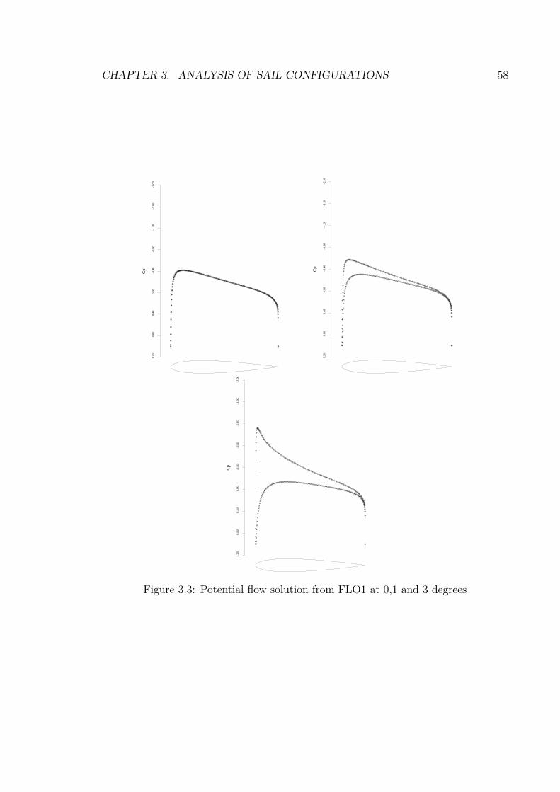
CHAPTER 3. ANALYSIS OF SAIL CONFIGURATIONS 58
NACA 0012 ALPHA 0.000
CL 0.0000 CD 0.0000 CM 0.0000
GRID 256
1.
20
0.80
0.
40
0.00
-0.
40 -
0.80
-1.
20 -
1.60
-2.
00
Cp
+
+++++++++
++++++++
++++++++++
++++++++++++
++++++++++++++
++++++++++++
+++++++++++++
+++++++++++++++++++++++++++++++++++++
+++++
+
+
+
+
+
+++++
+
+
+
+
+
+
+++++++++++++++++++
+++++++++++++++++++++++++++++++++++++++++++++++++++++++++++++++++++++++++++++++++++++++++++++++++++++
+
NACA 0012 ALPHA 1.000
CL 0.1206 CD 0.0000 CM -0.0013
GRID 256
1.
20
0.80
0.
40
0.00
-0.
40 -
0.80
-1.
20 -
1.60
-2.
00
Cp
+
+++++++++
++++++++
+++++++++++
++++++++++++++
+++++++++++++++
+++++++++++++++
+++++++++++++++++++++++++++++++++++++++++
+++++++
+
+
+
+++++
+
+
+
+
+
+
+
+
++++++++++++++++++++++++++++++++++++++++++++++++++++++++++++++++++++++++++++++++++++++++++++++++++++++++++++++++++++++
++
+
NACA 0012 ALPHA 3.000
CL 0.3617 CD 0.0000 CM -0.0040
GRID 256
1.
20
0.80
0.
40
0.00
-0.
40 -
0.80
-1.
20 -
1.60
-2.
00
Cp
+
+++++++++
++++++++
+++++++++++++
+++++++++++++++++++
+++++++++++++++++++++++++++
+++++++++++++++++++++++++++++++++++++++++++++++++
++
+
+
+
+
+
+
+
+
+++++++++++++++++++++++++++++++++++++++++++++++++++++++++++++++++++++++++++++++++++++++++++++++++++++++++++++++++++++++
++
+
Figure 3.3: Potential flow solution from FLO1 at 0,1 and 3 degrees

CHAPTER 3. ANALYSIS OF SAIL CONFIGURATIONS 59
NACA 0012 - SCHEME : QUAD. CELL-CENT. RHCUSP-SLIP MACH 0.000 ALPHA 0.000
CL 0.0000 CD -0.0001 CM 0.0000
GRID 161X33 NCYC 80 RES0.834E-03
0.1E
+01
0.8E
+00
0.4E
+00
-.2E
-15
-.4E
+00
-.8E
+00
-.1E
+01
-.2E
+01
-.2E
+01
Cp
+++++
++++++++++++++++++++++++++++++++++++++++++++++++++++++++++++++
+++++
+
+
+
+
+
+++++
++
+
+
+
+
+
++++++++++++++++++++
++++++++++++++++++++++++++++++++++++++++++++++++++++
NACA 0012 - SCHEME : QUAD. CELL-CENT. RHCUSP-SLIP MACH 0.000 ALPHA 1.000
CL 0.1199 CD 0.0000 CM -0.0013
GRID 161X33 NCYC 80 RES0.262E-02
0.1E
+01
0.8E
+00
0.4E
+00
-.2E
-15
-.4E
+00
-.8E
+00
-.1E
+01
-.2E
+01
-.2E
+01
Cp
+++++
++++++++++++++++++++++++++++++++++++++++++++++++++++++++++++
++++++++
+
+
++++++
+
+
+
+
+
+
+
++++++++++++++++++++++++++++++++++++++++++++++++++++++++++++++++++++++
+++
NACA 0012 - SCHEME : QUAD. CELL-CENT. RHCUSP-SLIP MACH 0.000 ALPHA 3.000
CL 0.3598 CD 0.0001 CM -0.0039
GRID 161X33 NCYC 80 RES0.734E-02
0.1E
+01
0.8E
+00
0.4E
+00
-.2E
-15
-.4E
+00
-.8E
+00
-.1E
+01
-.2E
+01
-.2E
+01
Cp
+++++
+++++++++++++++++++++++++++++++++++++++++++++++++++++++++
++++++++++++++++
+
+
+
+
+
+
+
+
+
++++++++++++++++++++++++++++++++++++++++++++++++++++++++++++++++++++++
++++
Figure 3.4: Flow over a NACA 0012 airfoil at 0,1 and 3 degrees using a cell-centeredscheme

CHAPTER 3. ANALYSIS OF SAIL CONFIGURATIONS 60
NACA 0012 MACH 0.000 ALPHA 0.000
CL 0.0006 CD 0.0003 CM -0.0001
GRID 161X33 NCYC 200 RES0.730E-07
0.1E
+01
0.8E
+00
0.4E
+00
-.2E
-15
-.4E
+00
-.8E
+00
-.1E
+01
-.2E
+01
-.2E
+01
Cp
++++++
+++++++++++++++++++++++++++++++++++++++++++++++++++++++++++++
++++++
+
+
+
+
+
+++++
+
+
+
+
+
+
++++++++++++++++++++++++++++++++++++++++++++++++++++++++++++++++++++++
+++
NACA 0012 MACH 0.000 ALPHA 1.000
CL 0.1200 CD 0.0003 CM -0.0014
GRID 161X33 NCYC 200 RES0.829E-07
0.1E
+01
0.8E
+00
0.4E
+00
-.2E
-15
-.4E
+00
-.8E
+00
-.1E
+01
-.2E
+01
-.2E
+01
Cp
++++++
++++++++++++++++++++++++++++++++++++++++++++++++++++++++++++
+++++++
+
+
+
+++++
++
+
+
+
+
+
+
+++++++++++++++++++++++++++++++++++++++++++++++++++++++++++++++++++++
++++
NACA 0012 MACH 0.000 ALPHA 3.000
CL 0.3587 CD 0.0005 CM -0.0040
GRID 161X33 NCYC 200 RES0.187E-06
0.1E
+01
0.8E
+00
0.4E
+00
-.2E
-15
-.4E
+00
-.8E
+00
-.1E
+01
-.2E
+01
-.2E
+01
Cp
+++++
++++++++++++++++++++++++++++++++++++++++++++++++++++++++++
+++++++++++++++
++
+
+
+
+
+
+
+
+
++++++++++++++++++++++++++++++++++++++++++++++++++++++++++++++++++++++
++++
Figure 3.5: Flow over a NACA 0012 airfoil at 0,1 and 3 degrees using a nodal scheme

CHAPTER 3. ANALYSIS OF SAIL CONFIGURATIONS 61
NACA 0012 - SCHEME : HALF-STAGGERED MACH 0.000 ALPHA 0.000
CL 0.0006 CD -0.0001 CM -0.0001
GRID 161X33 NCYC 150 RES0.169E-06
0.1E
+01
0.8E
+00
0.4E
+00
-.2E
-15
-.4E
+00
-.8E
+00
-.1E
+01
-.2E
+01
-.2E
+01
Cp
+++++
++++++++++++++++++++++++++++++++++++++++++++++++++++++++++++++
+++++
+
+
+
+
+
+++++
++
+
+
+
+
+
+++++++++++++++++++++++++++++++++++++++++++++++++++++++++++++++++++++
+++
NACA 0012 - SCHEME : HALF-STAGGERED MACH 0.000 ALPHA 1.000
CL 0.1211 CD -0.0001 CM -0.0014
GRID 161X33 NCYC 150 RES0.212E-06
0.1E
+01
0.8E
+00
0.4E
+00
-.2E
-15
-.4E
+00
-.8E
+00
-.1E
+01
-.2E
+01
-.2E
+01
Cp
+++++
++++++++++++++++++++++++++++++++++++++++++++++++++++++++++++
+++++++
+
+
+
++++++
+
+
+
+
+
+
+
++++++++++++++++++++++++++++++++++++++++++++++++++++++++++++++++++++++
+++
NACA 0012 - SCHEME : HALF-STAGGERED MACH 0.000 ALPHA 3.000
CL 0.3620 CD -0.0001 CM -0.0040
GRID 161X33 NCYC 150 RES0.366E-06
0.1E
+01
0.8E
+00
0.4E
+00
-.2E
-15
-.4E
+00
-.8E
+00
-.1E
+01
-.2E
+01
-.2E
+01
Cp
+++++
+++++++++++++++++++++++++++++++++++++++++++++++++++++++++
++++++++++++++++
+
+
+
+
+
+
+
+
+
+++++++++++++++++++++++++++++++++++++++++++++++++++++++++++++++++++++++
+++
Figure 3.6: Flow over a NACA 0012 airfoil at 0,1 and 3 degrees using a half-staggeredscheme

CHAPTER 3. ANALYSIS OF SAIL CONFIGURATIONS 62
0 20 40 60 80 100 120 140 160 180−7
−6
−5
−4
−3
−2
−1
0
1
2
3Total Pressure Error at 0 deg angle of attack
Points along the airfoil surface,Lower surface trailing edge to upper surface trailing edge
Per
cent
age
Err
or
cell−centercell−vertexhalf−staggerred
Figure 3.7: Total Pressure losses on the airfoil surface at 0o
0 20 40 60 80 100 120 140 160 180−6
−5
−4
−3
−2
−1
0
1
2
3
4Total Pressure Error at 1 deg angle of attack
Points along the airfoil surface,Lower surface trailing edge to upper surface trailing edge
Per
cent
age
Err
or
cell−centercell−vertexhalf−staggerred
Figure 3.8: Total Pressure losses on the airfoil surface at 1o
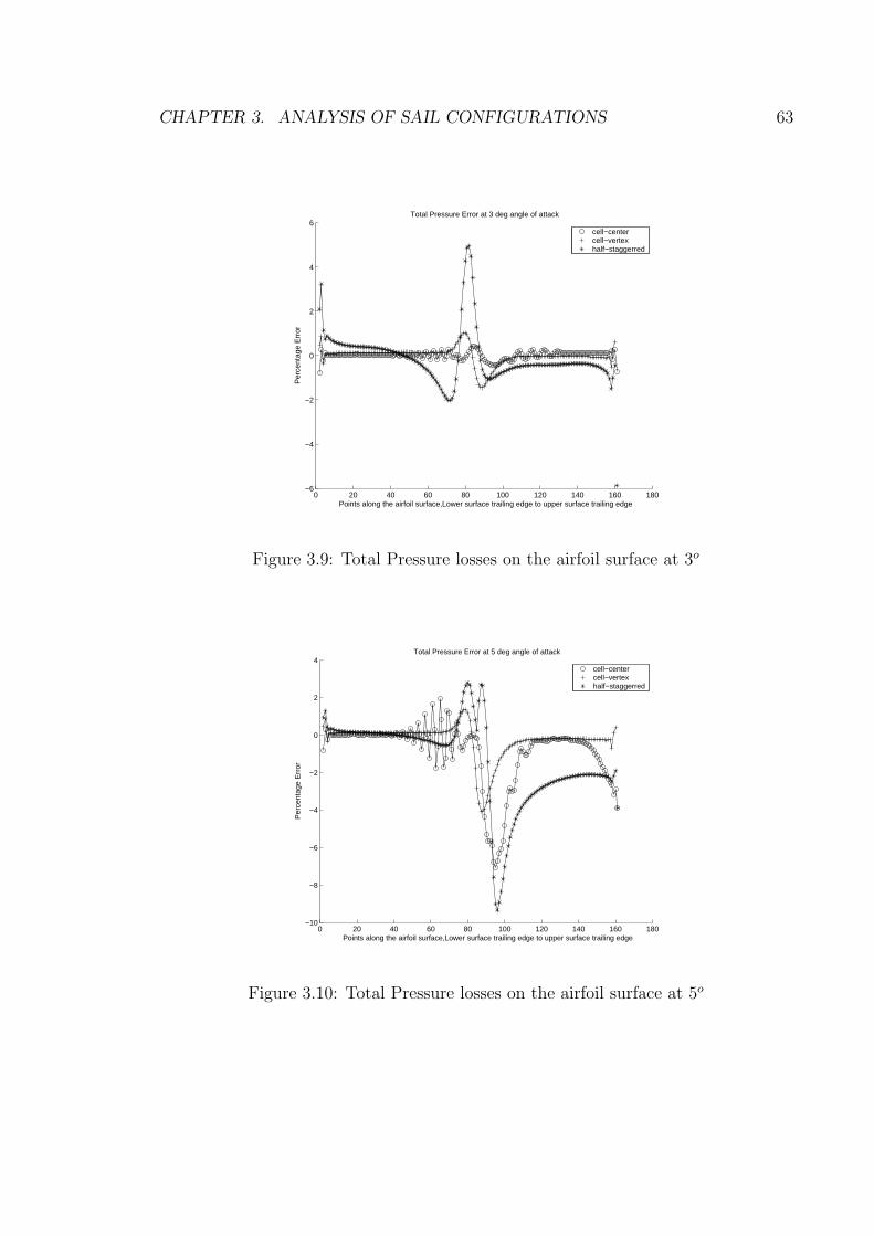
CHAPTER 3. ANALYSIS OF SAIL CONFIGURATIONS 63
0 20 40 60 80 100 120 140 160 180−6
−4
−2
0
2
4
6Total Pressure Error at 3 deg angle of attack
Points along the airfoil surface,Lower surface trailing edge to upper surface trailing edge
Per
cent
age
Err
or
cell−centercell−vertexhalf−staggerred
Figure 3.9: Total Pressure losses on the airfoil surface at 3o
0 20 40 60 80 100 120 140 160 180−10
−8
−6
−4
−2
0
2
4Total Pressure Error at 5 deg angle of attack
Points along the airfoil surface,Lower surface trailing edge to upper surface trailing edge
Per
cent
age
Err
or
cell−centercell−vertexhalf−staggerred
Figure 3.10: Total Pressure losses on the airfoil surface at 5o

CHAPTER 3. ANALYSIS OF SAIL CONFIGURATIONS 64
24 m
Twisted inflowwith boundary layerprofile
Main Sail
10 m
10 m
2.3 m
Jib
Figure 3.11: Sail geometry
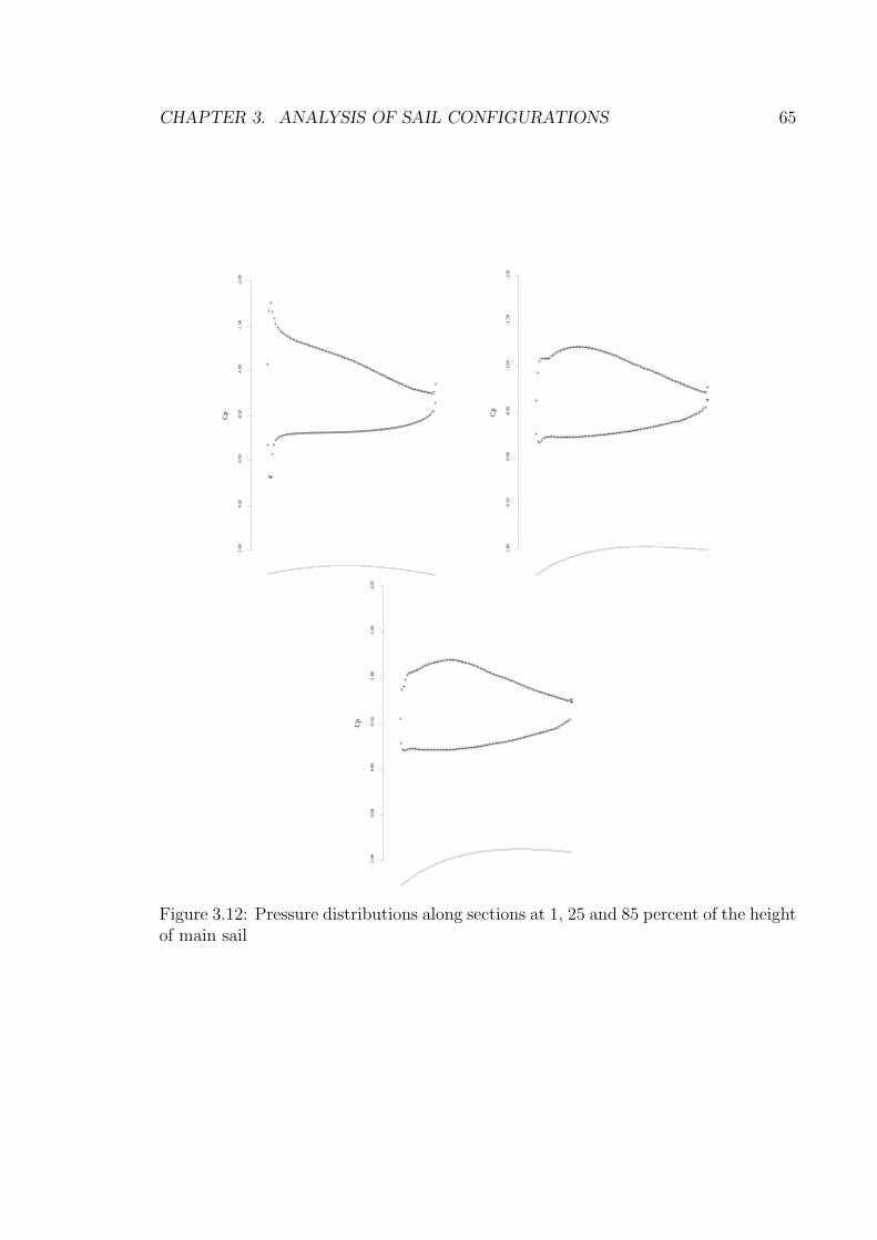
CHAPTER 3. ANALYSIS OF SAIL CONFIGURATIONS 65
M2F TNZ ALPHA 18.000 Z 0.023
CL 0.7986 CD 0.2178 CM -0.3186
NCYC 200 RES0.914E-01
1.
00
0.50
0.
00 -
0.50
-1.
00 -
1.50
-2.
00
Cp
+++++++++++++++++++++++++++++++++++++++++++++++++++++++++++++++++++++++++++++++++++++++++++++++
+
+
+++
+
+
+
+
++++++++++++++++++++++++++++++++++++++++++++++++++++++++++++++++++++++++++++++++++++++++++++++++
+
M2F TNZ ALPHA 18.000 Z 0.336
CL 0.7677 CD 0.0882 CM -0.3240
NCYC 200 RES0.914E-01
1.
00
0.50
0.
00 -
0.50
-1.
00 -
1.50
-2.
00
Cp
++++++++++++++++++++++++++++++++++++++++++++++++++++++++++++++++++++++++++++++++++++++++++++++++++++
+
+
+
++++++++++
+++++++++++++++++++++++++++++++++++++++++++++++++++++++++++++++++++++++++++++++++++++++
+
M2F TNZ ALPHA 18.000 Z 0.526
CL 0.7794 CD 0.0495 CM -0.3384
NCYC 200 RES0.914E-01
1.
00
0.50
0.
00 -
0.50
-1.
00 -
1.50
-2.
00
Cp
++
+++++++++++++++++++++++++++++++++++++++++++++++++++++++++++++++++++++++++++++++++++++++++++++++++++
+
+++++++
+++++++++
+++++++++++++++++++++++++++++++++++++++++++++++++++++++++++++++++++++++++++++++++++
Figure 3.12: Pressure distributions along sections at 1, 25 and 85 percent of the heightof main sail
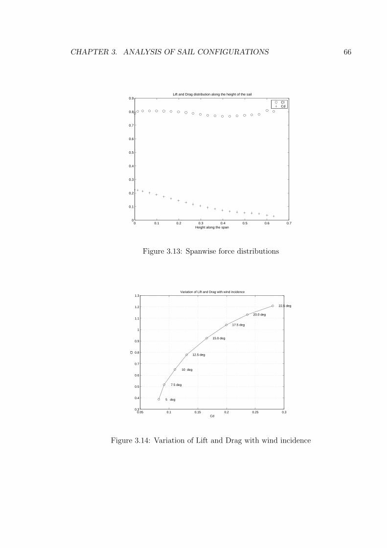
CHAPTER 3. ANALYSIS OF SAIL CONFIGURATIONS 66
0 0.1 0.2 0.3 0.4 0.5 0.6 0.70
0.1
0.2
0.3
0.4
0.5
0.6
0.7
0.8
0.9Lift and Drag distribution along the height of the sail
Height along the span
ClCd
Figure 3.13: Spanwise force distributions
0.05 0.1 0.15 0.2 0.25 0.30.3
0.4
0.5
0.6
0.7
0.8
0.9
1
1.1
1.2
1.3Variation of Lift and Drag with wind incidence
Cd
Cl
5 deg
7.5 deg
10 deg
12.5 deg
15.0 deg
17.5 deg
20.0 deg
22.5 deg
Figure 3.14: Variation of Lift and Drag with wind incidence
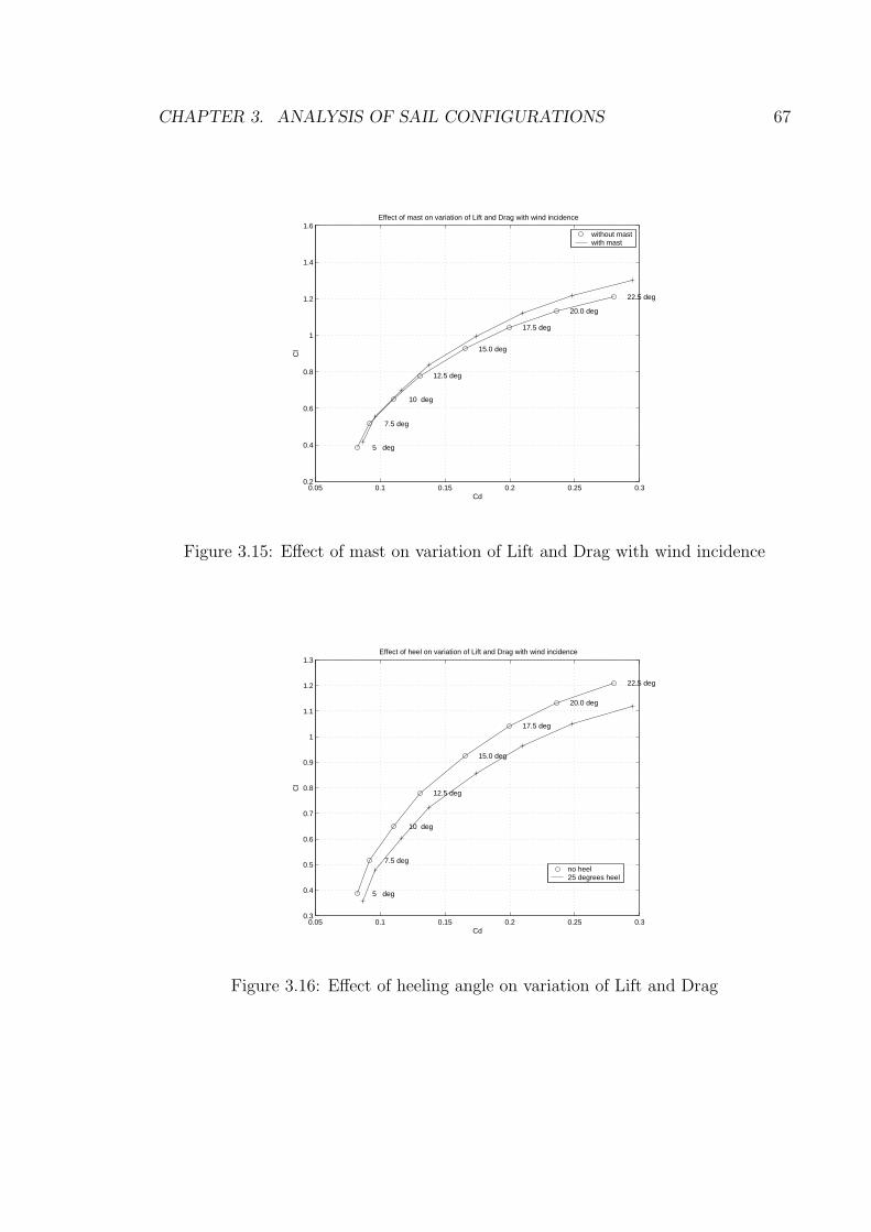
CHAPTER 3. ANALYSIS OF SAIL CONFIGURATIONS 67
0.05 0.1 0.15 0.2 0.25 0.30.2
0.4
0.6
0.8
1
1.2
1.4
1.6Effect of mast on variation of Lift and Drag with wind incidence
Cd
Cl
5 deg
7.5 deg
10 deg
12.5 deg
15.0 deg
17.5 deg
20.0 deg
22.5 deg
without mastwith mast
Figure 3.15: Effect of mast on variation of Lift and Drag with wind incidence
0.05 0.1 0.15 0.2 0.25 0.30.3
0.4
0.5
0.6
0.7
0.8
0.9
1
1.1
1.2
1.3Effect of heel on variation of Lift and Drag with wind incidence
Cd
Cl
5 deg
7.5 deg
10 deg
12.5 deg
15.0 deg
17.5 deg
20.0 deg
22.5 deg
no heel25 degrees heel
Figure 3.16: Effect of heeling angle on variation of Lift and Drag

CHAPTER 3. ANALYSIS OF SAIL CONFIGURATIONS 68
1 2 3 4 5 6 7 8 9 10 11 12
5
10
15
20
25
Height along the span
twist, camber and chord distribution of the head sail
twist distribution in degchord distribution in mcamber distribution as % of chord
Figure 3.17: Twist,camber and chord distribution of the head sail
10 15 20 25 30 35 40 45 50
0
5
10
15
20
Height along the span
twist, camber and chord distribution of the main sail
twist distribution in degchord distribution in mcamber distribution as % of chord
Figure 3.18: Twist,camber and chord distribution of the main sail

CHAPTER 3. ANALYSIS OF SAIL CONFIGURATIONS 69
M2F TNZ ALPHA 19.000 Z 2.587
CL 0.8872 CD 0.2378 CM -0.5607
NCYC 500 RES0.180E-07
1.
00
0.50
0.
00 -
0.50
-1.
00 -
1.50
-2.
00 -
2.50
-3.
00
Cp
++
+++++++++++++++++++++++++++++++
++
++
+++++ + + ++
++
++
+ + + + + + + + + + + + + + + + + + + + + + + + + + + + ++
+
M2F TNZ ALPHA 19.000 Z 9.509
CL 0.8018 CD 0.1745 CM -0.5067
NCYC 500 RES0.180E-07
1.
00
0.50
0.
00 -
0.50
-1.
00 -
1.50
-2.
00 -
2.50
-3.
00
Cp ++
++
+++++++++++++++++++++++++++++
++
++
+++++
+ + ++
++
++
++
++ + + + + + + + + + + + + + + + + + + + + + + + + +
+
+
M2F TNZ ALPHA 19.000 Z 16.409
CL 0.5918 CD 0.1136 CM -0.4305
NCYC 500 RES0.180E-07
1.
00
0.50
0.
00 -
0.50
-1.
00 -
1.50
-2.
00 -
2.50
-3.
00
Cp ++
++
++++++++++++++++++++++++++++
++
++++
+++
++
+ + + ++
++
++
++ + + + + + + + + + + + + + + + + + + + + + + + + +
++
Figure 3.19: Pressure distributions along sections at 1, 25 and 85 percent of the heightof head sail
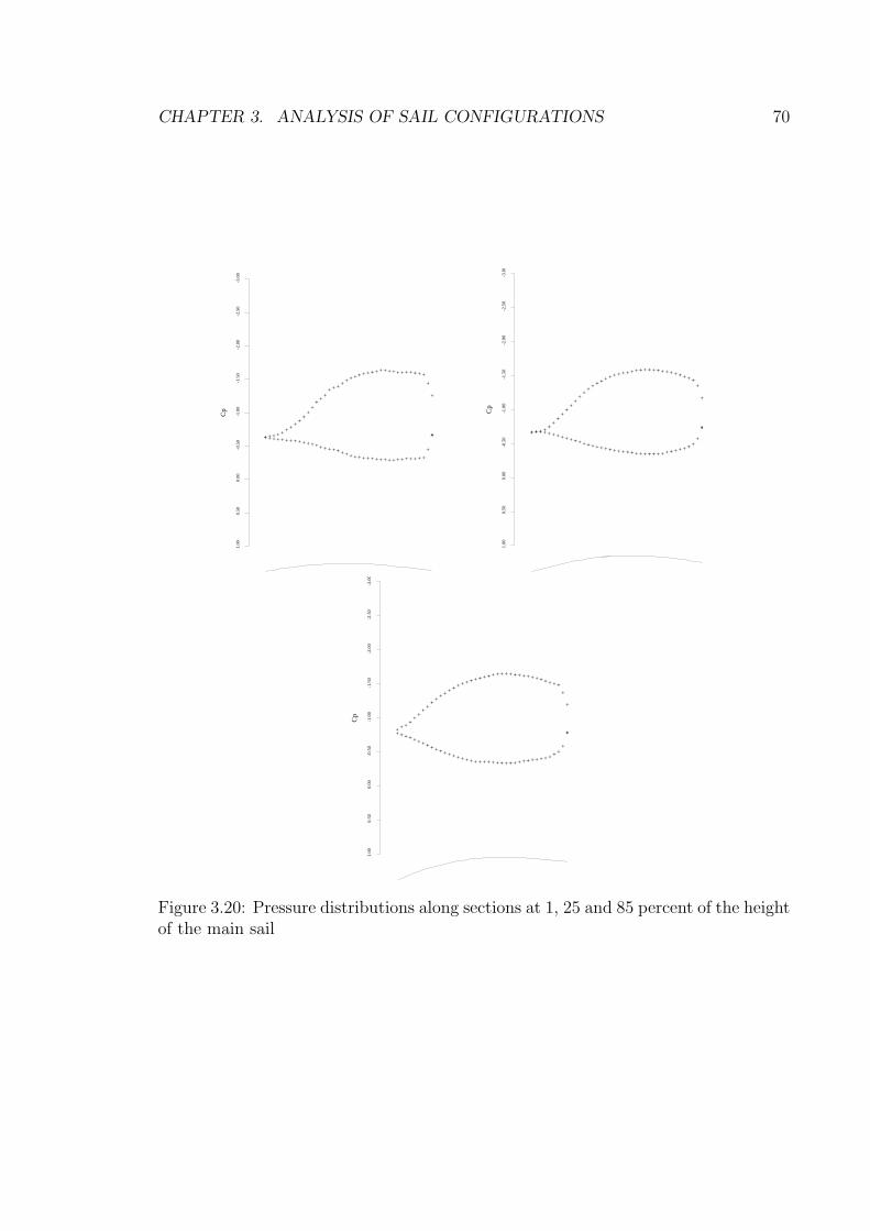
CHAPTER 3. ANALYSIS OF SAIL CONFIGURATIONS 70
M2F TNZ ALPHA 19.000 Z 3.885
CL 0.8119 CD 0.3222 CM -0.5526
NCYC 500 RES0.180E-07
1.
00
0.50
0.
00 -
0.50
-1.
00 -
1.50
-2.
00 -
2.50
-3.
00
Cp
++
++++++++++++++++++++++++++++++++++++++++ + + + + + + +
++
++
++
++ + + + + + + + + + + + + + + + + + + + + + +
+
+
M2F TNZ ALPHA 19.000 Z 10.532
CL 0.7847 CD 0.2737 CM -0.5064
NCYC 500 RES0.180E-07
1.
00
0.50
0.
00 -
0.50
-1.
00 -
1.50
-2.
00 -
2.50
-3.
00
Cp
++
++++++++++++++++++++++++++++++++++++++++ + + + +
++
++
++
++
+ + + + + + + + + + + + + + + + + + + + + + + + ++
+
M2F TNZ ALPHA 19.000 Z 18.929
CL 0.9173 CD 0.2608 CM -0.5521
NCYC 500 RES0.180E-07
1.
00
0.50
0.
00 -
0.50
-1.
00 -
1.50
-2.
00 -
2.50
-3.
00
Cp
++
+++++++++++++++++++++++++++++++++++++++
+ + + ++
++
++
+ + + + + + + + + + + + + + + + + + + + + + + + + + + + ++
+
Figure 3.20: Pressure distributions along sections at 1, 25 and 85 percent of the heightof the main sail

CHAPTER 3. ANALYSIS OF SAIL CONFIGURATIONS 71
0 5 10 15 20 25−0.2
0
0.2
0.4
0.6
0.8
1
1.2Lift and Drag distribution along the height of the head sail
Height along the span
ClCd
Figure 3.21: Spanwise force distributions on the head sail
0 5 10 15 20 25 30 350
0.2
0.4
0.6
0.8
1
1.2
1.4Lift and Drag distribution along the height of the head sail
Height along the span
ClCd
Figure 3.22: Spanwise force distributions on the main sail
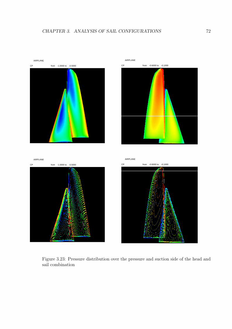
CHAPTER 3. ANALYSIS OF SAIL CONFIGURATIONS 72
AIRPLANE CP from -1.0000 to -0.5000
AIRPLANE CP from -0.6000 to -0.1000
AIRPLANE CP from -1.0000 to -0.5000
AIRPLANE CP from -0.6000 to -0.1000
Figure 3.23: Pressure distribution over the pressure and suction side of the head andsail combination

CHAPTER 3. ANALYSIS OF SAIL CONFIGURATIONS 73
2 4 6 8 10 12 14−0.5
0
0.5
1
1.5
2
Z = 25
Deformed and original section geometry along the height of the head sail
Z = 18Z = 14Z = 8Z = 3.6
OriginalDeformed
Figure 3.24: Original and deformed sail sections for the head sail
10 11 12 13 14 15 16 17 18 19 20−0.2
0
0.2
0.4
0.6
0.8
1
1.2
Z = 5
Z = 8.5
Z = 14
Z = 19
Z = 24
Z = 31
Deformed and original section geometry along the height of the main sail
OriginalDeformed
Figure 3.25: Original and deformed sail sections for the main sail

CHAPTER 3. ANALYSIS OF SAIL CONFIGURATIONS 74
M2F TNZ ALPHA 19.000 Z 2.587
CL 0.8897 CD 0.1600 CM -0.4765
NCYC 500 RES0.538E-02
1.
00
0.50
0.
00 -
0.50
-1.
00 -
1.50
-2.
00 -
2.50
-3.
00
Cp ++
++++++++++++++++++++++++++++++++++++++
+
++ + +
+ ++ + + + + + + + + + + + + + + + + + + + + + + + + + + + + + + + + +
M2F TNZ ALPHA 19.000 Z 9.509
CL 1.0856 CD 0.0757 CM -0.5412
NCYC 500 RES0.538E-02
1.
00
0.50
0.
00 -
0.50
-1.
00 -
1.50
-2.
00 -
2.50
-3.
00
Cp
++
+++++++++++++++++++++++++++++++++++
++
++
++
++
++
++
++ + + + + + + + + + + + + + + + + + + + + + + + + + + + + + +
M2F TNZ ALPHA 19.000 Z 16.409
CL 1.0096 CD -0.0163 CM -0.5429
NCYC 500 RES0.538E-02
1.
00
0.50
0.
00 -
0.50
-1.
00 -
1.50
-2.
00 -
2.50
-3.
00
Cp
+++++
++
++++++++++++++++++++++++++++++
+++++ + +
++
++
++
++
+ + + + + + + + + + + + + + + + + + + + + + + + + + + ++
Figure 3.26: Pressure distributions along sections at 1, 25 and 85 percent of the heightof head sail after aeroelastic analysis

CHAPTER 3. ANALYSIS OF SAIL CONFIGURATIONS 75
M2F TNZ ALPHA 19.000 Z 3.885
CL 0.7112 CD 0.2590 CM -0.4177
NCYC 500 RES0.538E-02
1.
00
0.50
0.
00 -
0.50
-1.
00 -
1.50
-2.
00 -
2.50
-3.
00
Cp
++++++++++++++++++++++++++++++++++++++
+++
++ + + + + + + +
++
+ + + + + + + + + + + + + + + + + + + + + + + + + + ++
+
M2F TNZ ALPHA 19.000 Z 10.532
CL 0.9060 CD 0.2505 CM -0.4739
NCYC 500 RES0.538E-02
1.
00
0.50
0.
00 -
0.50
-1.
00 -
1.50
-2.
00 -
2.50
-3.
00
Cp
+++
++++++++++++++++++++++++++++++++++++
+
+
+
+ + + + + + + ++
+ + + + + + + + + + + + + + + + + + + + + + + + ++
+ ++
+
M2F TNZ ALPHA 19.000 Z 18.929
CL 1.1717 CD 0.2199 CM -0.5570
NCYC 500 RES0.538E-02
1.
00
0.50
0.
00 -
0.50
-1.
00 -
1.50
-2.
00 -
2.50
-3.
00
Cp
+++++++++++++++++++++++++++++++++++++++
+
+
+
++
+ + + + + + + + + + + + + + + + + + + + + + + + + + + + + + + + + + + ++
Figure 3.27: Pressure distributions along sections at 1, 25 and 85 percent of the heightof main sail after aeroelastic analysis

Chapter 4
Aerodynamic Shape optimization
With the availability of high performance computing platforms and robust numerical
methods to simulate fluid flows, it is possible to shift attention to automated design
procedures which use CFD combined with gradient-based optimization techniques.
Typically, in gradient-based optimization techniques, a control function to be opti-
mized (the sail shape, for example) is parameterized with a set of design variables
and a suitable cost function to be minimized is defined. For aerodynamic problems,
the cost function may be the lift or drag or a specified target pressure distribution.
Then, a constraint, the governing equations, can be introduced in order to express
the dependence between the cost function and the control function. The sensitivity
of the cost function with respect to the design variables are calculated in order to
get a direction of improvement. Finally, a step is taken in this direction and the
procedure is repeated until convergence is achieved. Finding a fast and accurate way
of calculating the necessary gradient information is essential to developing an effec-
tive design method since this can be the most time consuming portion of the design
process. This is particularly true in problems which involve a very large number of
design variables as is the case in a typical three dimensional sail shape design.
The control theory approach has dramatic computational cost advantages over
the finite-difference method of calculating gradients. The control theory approach
is also called the adjoint method as the necessary gradients are obtained through
the solution of an adjoint system of equations of the governing equations of interest.
76

CHAPTER 4. AERODYNAMIC SHAPE OPTIMIZATION 77
The adjoint method is extremely efficient since the computational expense incurred
in the calculation of the complete gradient is effectively independent of the number of
design variables. Control theory was applied in this way to shape design for elliptic
equations by Pironneau [50] and to transonic flow by Jameson [42].
In this study, a continuous adjoint formulation has been used to derive the adjoint
system of equations. Hence, the adjoint equations are derived directly from the
governing equations and then discretized. This approach has the advantage over the
discrete adjoint formulation in that the resulting adjoint equations are independent
of the form of discretized flow equations. The adjoint system of equations has a
similar form to the governing equations of the flow and hence the numerical methods
discussed in the previous chapters can be reused for the adjoint equations. The
gradient formulation is derived to be independent of the mesh modification which is
critical for this design methodology to work on unstructured meshes. If the gradient
depends on the form of the mesh modification, then the field integral in the gradient
calculation has to be recomputed for mesh modifications corresponding to each design
variable. Using the gradients computed with this new formulation, a steepest descent
method is used to improve an existing design.
4.1 The general formulation of the Adjoint Ap-
proach to Optimal Design
The aerodynamic properties which define the cost function are functions of the flow-
field variables, w, and the physical location of the boundary, which may be represented
by the function, F . Then
I = I(w,F),
and the variation of the cost function can be expressed as
δI =∂IT
∂wδw +
∂IT
∂F δF . (4.1)

CHAPTER 4. AERODYNAMIC SHAPE OPTIMIZATION 78
Using control theory, the governing equations of the flow field are introduced as a
constraint in such a way that the final expression for the gradient does not require
re-evaluation of the flow-field. In order to achieve this, δw must be eliminated from
equation (4.1). Suppose that the governing equation, R, which expresses the depen-
dence of w and F within the flow field domain D can be written as
R(w,F) = 0. (4.2)
Then δw is determined from the expression for the variation in R
δR =
[∂R
∂w
]δw +
[∂R
∂F]δF = 0. (4.3)
Next, introducing a Lagrange Multiplier ψ, we have
δI =∂IT
∂wδw +
∂IT
∂F δF − ψT
([∂R
∂w
]δw +
[∂R
∂F]δF
),
which can be rearranged as
δI =
(∂IT
∂w− ψT
[∂R
∂w
])δw +
(∂IT
∂F − ψT
[∂R
∂F])
δF ,
Choosing ψ to satisfy the adjoint equation
[∂R
∂w
]T
ψ =∂I
∂w, (4.4)
the first term is eliminated and hence
δI = GδF , (4.5)
where
G =∂IT
∂F − ψT
[∂R
∂F]. (4.6)
CHAPTER 4. AERODYNAMIC SHAPE OPTIMIZATION 79
In this way the gradient with respect to the shape is obtained at the cost of one flow
and one adjoint solution.
After taking a step in the negative gradient direction, the gradient is recalculated
and the process is repeated to follow the path of steepest descent until a minimum
is reached. In order to avoid violating constraints the gradient can be projected into
an allowable subspace within which the constraints are satisfied. In this way one can
devise procedures which must necessarily converge at least to a local minimum and
which can be accelerated by the use of more sophisticated descent methods such as
conjugate gradient or quasi-Newton algorithms.
4.2 Adjoint and Gradient formulations
In applying the adjoint method one may apply the above procedure directly to the
partial differential equations to derive a continuous adjoint equation, which must then
be discretized to obtain a numerical solution. Alternatively one may derive a discrete
adjoint equation directly after first discretizing the flow equations. In this work the
first procedure has been adopted because it allows more flexibility in the formulation
of the gradient.
The procedure is illustrated here for the Euler equations. These are represented
in transformed coordinates ξi on a fixed computational domain.
Let
S = JK−1,
where
Kij =∂xi
∂ξj, J = det(K),
Then the transformed equations are
∂Fi
∂ξi=∂(Sijfj)
∂ξi= 0.
Consider the case of an inverse problem where one wishes to find the shape which
brings the pressure as close as possible to the specified target pressure, pt. Hence, the

CHAPTER 4. AERODYNAMIC SHAPE OPTIMIZATION 80
cost function has the form
I =1
2
∫
B(p− pt)
2dS
over the design surface B, which for convenience is assumed to be the surface ξ2 = 0.
Now a shape modification induces a change δp in the pressure and consequently
δI =
∫
B(p− pt)δpdS +
1
2
∫
B(p− pt)
2dδS.
The variation in the flow solution can be expressed as
∂
∂ψi
(δFi(w)) = 0.
Here the flux changes are
δFi = δSijfj + Ciδw,
where
Ci = Sij∂fj
∂w.
Consequently one can augment the cost variation by
∫
DψT ∂δFi
∂ξidξ,
which can be integrated by parts to obtain
∫
DψT ∂δFi
∂ξidξ =
∫
Bniψ
T δFidξB −∫
D
∂ψT
∂ξδFidξ.
Now choose ψ to satisfy the adjoint equation
CTi
∂ψ
∂ξi= 0,

CHAPTER 4. AERODYNAMIC SHAPE OPTIMIZATION 81
with the boundary condition
ψ2ηx + ψ3ηy + ψ4ηz = p− pt,
where ηx, ηy, ηz are the components of the surface normal. Then the boundary inte-
grals involving δp and the field integral involving δw are eliminated and the gradient
is reduced to
1
2
∫
B(p− pt)
2dδS −∫ ∫
B(δS21ψ2 + δS22ψ3 + δS23ψ4) pdξ1dξ3 −
∫
D
∂ψT
∂ξ(δSijfj)dξ,
where typically the first term is negligible and can be dropped.
The evaluation of the field integral requires the evaluation of the metric variations
δSij throughout the domain. The true gradient should not depend on the way the
mesh is modified. Consider the case of a mesh variation with a fixed boundary. Then
δI = 0,
but there is a variation in the transformed flux
δFi = δSijfj + Sij∂fj
∂wδw.
Here the true solution is unchanged, so the variation δw is actually the variation δw∗
due to the mesh movement δx at fixed ξ. Therefore
δw = δw∗ =∂w
∂xj
δxj,
and since∂δFi
∂ξ= 0,
it follows that ∫
DψT ∂(δSijfj)
∂ξidξ = −
∫
DψTSij
∂fj
∂wδw∗dξ,

CHAPTER 4. AERODYNAMIC SHAPE OPTIMIZATION 82
or ∫
DψT ∂(δSijfj)
∂ξidξ =
∫
DCi∂w
∂xj
δxjdξ.
A similar relationship can be derived in the general case with boundary movement [73].
Now,
∫
DψT δRdξ =
∫
D
∂
∂ξiCi(δw − δw∗)dξ
=
∫
D
∂ψT
∂ξiCi(δw − δw∗)dξ
=
∫
BψTCi(δw − δw∗)dξB. (4.7)
Hence on the wall boundary
C2δw = δF2 − δS2jfj.
Thus by choosing ψ to satisfy the adjoint equation and the adjoint boundary
condition, we have the following expression for the reduced gradient:
δI =
∫ ∫
BψT (δS2jfj + C2δw
∗)dξ1dξ3 −∫ ∫
B(δS21ψ2 + δS22ψ3 + δS23ψ4)pdξ1dξ3 (4.8)
It has been confirmed in numerical experiments performed by Jameson and Kim [73]
that these alternate formulations yield computed values of the gradient which are in
close agreement, and that the optimization procedure converges to essentially the
same result whichever is used. On a structured mesh one can explicitly define mesh
deformations which allow the field terms to be evaluated easily. On an unstructured
mesh this is not the case and the reduction to a boundary integral yields large sav-
ings in the computational cost. The discrete adjoint does not provide for such a
transformation.

CHAPTER 4. AERODYNAMIC SHAPE OPTIMIZATION 83
4.2.1 Adjoint Equations for the Euler equations modified by
the artificial compressibility method
Although the adjoint equation represents a linear set of partial differential equations
for the adjoint variables, they are of the same form of the flow equations. The
numerical solution procedures developed for the flow equations are applied to the
adjoint system with the appropriate boundary conditions. The adjoint co-state flux
terms are modified to account for the introduction of the artificial compressibility
terms in the governing flow equations. The methodology followed here is derived
from the work of Cowles and Martinelli [74]. The adjoint field equations can be
expressed as a time dependent system of the form
∂ψ
∂t− [Ai]
T ∂ψ
∂xi
= 0, (4.9)
where
ψ =
p
φ1
φ2
φ3
. (4.10)
Hence, this system can be integrated to steady state using a preconditioner similar
to that used in the method of artificial compressibility. The adjoint ‘continuity’
equation is augmented by a time derivative of the adjoint pressure p to
∂p
∂t− Γ2∂φi
∂xi
= 0. (4.11)
The form of Γ is identical to that used for the flow equations since the magnitude
of the eigenvalues of the flux Jacobians for the two systems are identical. Together
with equation (4.11), the adjoint system is discretized and solved in a manner that is
consistent with that used for the flow equation.

CHAPTER 4. AERODYNAMIC SHAPE OPTIMIZATION 84
4.2.2 The need for a Sobolev inner product in the definition
of the gradient
Another key issue for successful implementation of the continuous adjoint method is
the choice of an appropriate inner product for the definition of the gradient. It turns
out that there is an enormous benefit from the use of a modified Sobolev gradient,
which enables the generation of a sequence of smooth shapes. This can be illustrated
by considering the simplest case of a problem in calculus of variations [55].
Choose y(x) to minimize
I =
b∫
a
F (y, y′)dx,
with fixed end points y(a) and y(b). Under a variation δy(x),
δI =
b∫
a
(∂F
∂yδy +
∂F
∂y′δy
′)dx
=
b∫
a
(∂F
∂y− d
dx
∂F
∂y′
)δydx.
Thus defining the gradient as
g =∂F
∂y− d
dx
∂F
∂y′,
and the inner product as
(u, v) =
b∫
a
uvdx,
we find that
δI = (g, δy),
Then if we set
δy = −λg, λ > 0,
CHAPTER 4. AERODYNAMIC SHAPE OPTIMIZATION 85
we obtain an improvement
δI = −λ(g, g) ≤ 0,
unless g = 0, the necessary condition for a minimum. Note that g is a function of
y, y′, y
′′,
g = g(y, y′, y
′′),
Now each step
yn+1 = yn − λngn
reduces the smoothness of y by two classes. Thus the computed trajectory becomes
less and less smooth, leading to instability.
In order to prevent this we can introduce a modified Sobolev inner product [72]
〈u, v〉 =
∫(uv + εu
′v′)dx,
where ε is a parameter that controls the weight of the derivatives. If we define a
gradient g such that
δI = 〈g, δy〉,
Then we have
δI =
∫(gδy + εg
′δy
′)dx
=
∫(g − ∂
∂xε∂g
∂x)δydx
= (g, δy) ,
where
g − ∂
∂xε∂g
∂x= g,
and g = 0 at the end points. Thus g is obtained from g by a smoothing equation.
Now the step
yn+1 = yn − λngn
CHAPTER 4. AERODYNAMIC SHAPE OPTIMIZATION 86
gives an improvement
δI = −λn〈gn, gn〉,
but yn+1 has the same smoothness as yn, resulting in a stable process.
In applying control theory for aerodynamic shape optimization, the use of a
Sobolev gradient is equally important for the preservation of the smoothness class
of the redesigned surface and it has been employed to obtain all the results in the
next chapter.
4.3 Analysis of the Optimization Procedure
Once the gradient has been determined, any number of optimization algorithms can be
utilized to determine the desired shape modification. In this work, a steepest descent
method is used in which small steps are taken in the negative gradient direction
δF = −λG
This can be thought of as a simulation of the following time dependent process [75]
dFdt
= −G,
where the λ is the time step ∆t. Let A be the Hessian matrix with element
Aij =∂Gi
∂Fi
=∂2I
∂Fi∂Fj
.
Suppose that a locally minimum value of the cost function I∗ = I(F) is attained
when F = F∗. Then the gradient G∗ = G(F) must be zero, while the Hessian matrix
A∗ = A(F) must be positive definite. Since G∗ is zero, the cost function can be
expanded as a Taylor series in the neighborhood of F∗ with the form
I(F) = I∗ +1
2(F − F∗)A(F − F∗) + ...
CHAPTER 4. AERODYNAMIC SHAPE OPTIMIZATION 87
Correspondingly,
G(F) = A(F − F∗) + ...
As F approaches F∗, the leading terms become dominant. Then, setting F , the
search process approximatesdF
dt= −A∗F
Also, since A∗ is positive definite it can be expanded as
A∗ = RMRT ,
where M is a diagonal matrix containing the eigenvalues of A∗, and
RRT = RTR = I.
Setting
v = RTF ,
the search process can be represented as
dv
dt= −Mv.
The stability region for the forward Euler time stepping scheme is a unit circle centered
at -1 on the negative real axis. Thus for stability we must choose
µmax∆t = µmaxλ < 2,
while the asymptotic decay rate, given by the smallest eigenvalue, is proportional to
e−µmint. In order to improve the rate of convergence, one can set
δF = λPG,
where P is a preconditioner for the search. An ideal choice is P = A−1, so that the

CHAPTER 4. AERODYNAMIC SHAPE OPTIMIZATION 88
corresponding time dependent process reduces to
dF
dt= −F,
for which all eigenvalues are equal to unity, and F is reduced to zero in one time step
by the choice δt = 1.
With problems of the present complexity the calculation of the Hessian is com-
putationally infeasible. However, the smoothing operator which maps the gradient
to a Sobolev space proves to be a very effective preconditioner, and it is used in the
present work.
4.4 Mesh movement
The same tools used for mesh deformation during the aeroelastic analysis are reused
to induce mesh modifications during the design cycle. Due to the nature and the
magnitude of the geometry modifications, the spring method provides reasonable
answers. As in the aeroelastic analysis, the solution of the elasticity equations provides
a more robust tool to perform mesh modifications. However, the solution of the
elasticity equations is computationally more expensive. Hence, the spring method
has been used to obtain the results presented in the next chapter.
4.5 Parallel Implementation
The modules and data structures developed to solve the flow equations are reused to
solve the adjoint system in parallel. The gradient calculation and the mesh movement
are also executed in parallel though these are relatively inexpensive steps in the
optimization strategy. The parallel implementation of the design methodology enables
inverse design problems for incompressible flows to be performed in about 30 minutes
(for a mesh with 300000 nodes) using 8 processors of an SGI Origin 300.

Chapter 5
Validation of the Optimization
Procedure and Results
The aerodynamic shape optimization procedure for unstructured grids and the re-
duced gradient formulation described in the previous chapter were used to obtain the
optimal shape of sail geometries. To validate the design procedure, the method was
initially applied to airfoils and wings in compressible flows where comparative data
is available from previously developed structured grid codes [58].
In the following sections, two dimensional shape optimization of airfoils in tran-
sonic flows are presented first. Then, using the idea of artificial compressibility, the
flow and the adjoint equations are modified to perform shape optimization of airfoils
in incompressible flow. Three dimensional flows around wing geometries were then
investigated. Wings in transonic flows were initially investigated to validate the de-
sign process and then the flow and adjoint equations were modified to redesign wings
in incompressible flow. After proving the feasibility of the design methodology, sail
geometries were redesigned to remove the sharp suction peaks that were observed in
the flying shapes obtained by the aeroelastic simulations.
89
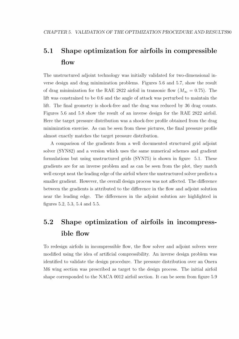
CHAPTER 5. VALIDATION OF THE OPTIMIZATION PROCEDURE AND RESULTS90
5.1 Shape optimization for airfoils in compressible
flow
The unstructured adjoint technology was initially validated for two-dimensional in-
verse design and drag minimization problems. Figures 5.6 and 5.7, show the result
of drag minimization for the RAE 2822 airfoil in transonic flow (M∞ = 0.75). The
lift was constrained to be 0.6 and the angle of attack was perturbed to maintain the
lift. The final geometry is shock-free and the drag was reduced by 36 drag counts.
Figures 5.6 and 5.8 show the result of an inverse design for the RAE 2822 airfoil.
Here the target pressure distribution was a shock-free profile obtained from the drag
minimization exercise. As can be seen from these pictures, the final pressure profile
almost exactly matches the target pressure distribution.
A comparison of the gradients from a well documented structured grid adjoint
solver (SYN82) and a version which uses the same numerical schemes and gradient
formulations but using unstructured grids (SYN75) is shown in figure 5.1. These
gradients are for an inverse problem and as can be seen from the plot, they match
well except neat the leading edge of the airfoil where the unstructured solver predicts a
smaller gradient. However, the overall design process was not affected. The difference
between the gradients is attributed to the difference in the flow and adjoint solution
near the leading edge. The differences in the adjoint solution are highlighted in
figures 5.2, 5.3, 5.4 and 5.5.
5.2 Shape optimization of airfoils in incompress-
ible flow
To redesign airfoils in incompressible flow, the flow solver and adjoint solvers were
modified using the idea of artificial compressibility. An inverse design problem was
identified to validate the design procedure. The pressure distribution over an Onera
M6 wing section was prescribed as target to the design process. The initial airfoil
shape corresponded to the NACA 0012 airfoil section. It can be seem from figure 5.9
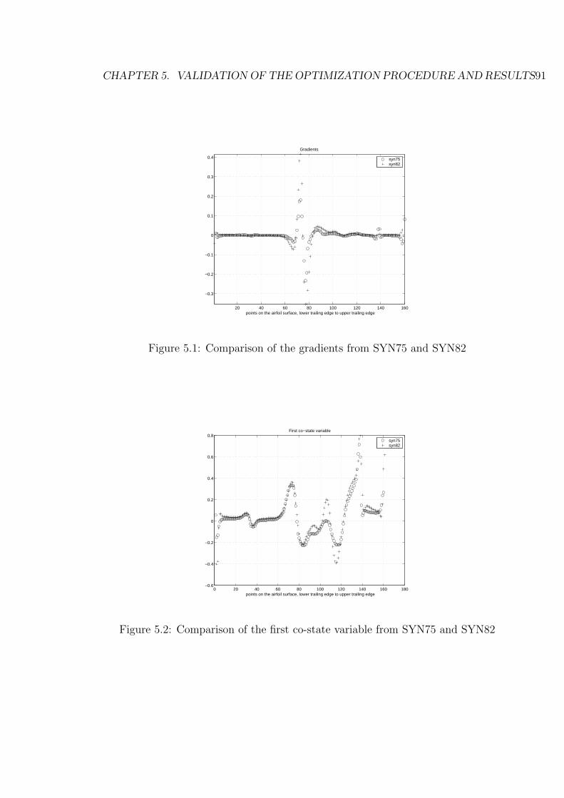
CHAPTER 5. VALIDATION OF THE OPTIMIZATION PROCEDURE AND RESULTS91
20 40 60 80 100 120 140 160
−0.3
−0.2
−0.1
0
0.1
0.2
0.3
0.4
Gradients
points on the airfoil surface, lower trailing edge to upper trailing edge
syn75syn82
Figure 5.1: Comparison of the gradients from SYN75 and SYN82
0 20 40 60 80 100 120 140 160 180−0.6
−0.4
−0.2
0
0.2
0.4
0.6
0.8First co−state variable
points on the airfoil surface, lower trailing edge to upper trailing edge
syn75syn82
Figure 5.2: Comparison of the first co-state variable from SYN75 and SYN82

CHAPTER 5. VALIDATION OF THE OPTIMIZATION PROCEDURE AND RESULTS92
0 20 40 60 80 100 120 140 160 180−2
−1.5
−1
−0.5
0
0.5
1Second co−state variable
points on the airfoil surface, lower trailing edge to upper trailing edge
syn75syn82
Figure 5.3: Comparison of the second co-state variable from SYN75 and SYN82
0 20 40 60 80 100 120 140 160 180−2
−1.5
−1
−0.5
0
0.5
1Third co−state variable
points on the airfoil surface, lower trailing edge to upper trailing edge
syn75syn82
Figure 5.4: Comparison of the third co-state variable from SYN75 and SYN82

CHAPTER 5. VALIDATION OF THE OPTIMIZATION PROCEDURE AND RESULTS93
20 40 60 80 100 120 140 160
−0.2
−0.1
0
0.1
0.2
0.3
Fourth co−state variable
points on the airfoil surface, lower trailing edge to upper trailing edge
syn75syn82
Figure 5.5: Comparison of the fourth co-state variable from SYN75 and SYN82
RAE 2822 MACH 0.750 ALPHA 0.703
CL 0.5999 CD 0.0062 CM -0.1334
GRID 161X33 NDES 0 RES0.785E-05 GMAX 0.000E+00
0.1E
+01
0.8E
+00
0.4E
+00
-.2E
-15
-.4E
+00
-.8E
+00
-.1E
+01
-.2E
+01
-.2E
+01
Cp
+++++++++++++++++++++
++
++
++
++
++
+++++++++++++++++++++++++++++++++++++++++++
+
+
+
+
+
+
+
+
++++++++++++++
+++++++++
++++++++
+++++++++++++++++++++++++
+
++++++++++++++++++++++
+
Figure 5.6: Initial pressure distribution for the RAE-2822 airfoil
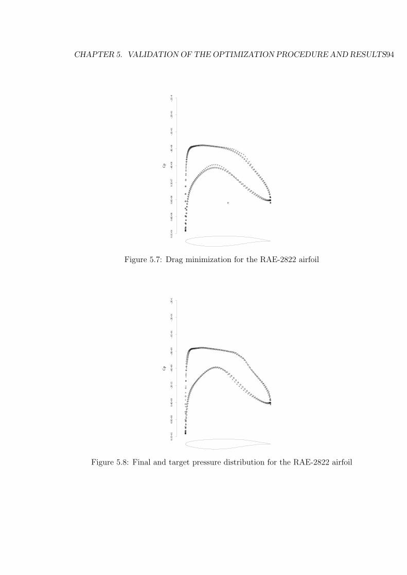
CHAPTER 5. VALIDATION OF THE OPTIMIZATION PROCEDURE AND RESULTS94
RAE 2822 MACH 0.750 ALPHA 0.866
CL 0.6000 CD 0.0026 CM -0.1243
GRID 161X33 NDES 40 RES0.191E-04 GMAX 0.569E-02
0.1E
+01
0.8E
+00
0.4E
+00
0.3E
-07
-.4E
+00
-.8E
+00
-.1E
+01
-.2E
+01
-.2E
+01
Cp
+++++++++++++++++++
++
++
++
++
++++++++++++++++++++++++++++++++++++++++++++++
+
+
+
+
+
+
+
+
+
++++++++++++++++++++
+++++++++++++++++++++++++++++++++++++++
++
++
++
++++++++++++++
+oooooooooooooooooooo
oo
oo
oo
ooooooooooooooooooooooooooooooooooooooooooooooo
o
o
o
o
o
o
o
o
ooooooooooooooooooo
oooooooooooooooooooooooooooooooooooooooo
oo
oo
oo
oooooooooooooo
o
Figure 5.7: Drag minimization for the RAE-2822 airfoil
RAE 2822 : INVERSE TO SHOCK FREE SOLUTION MACH 0.750 ALPHA 0.763
CL 0.6000 CD 0.0025 CM -0.1242
GRID 161X33 NDES 40 RES0.466E-05 GMAX 0.255E-02
0.1E
+01
0.8E
+00
0.4E
+00
-.2E
-15
-.4E
+00
-.8E
+00
-.1E
+01
-.2E
+01
-.2E
+01
Cp
++++++++++++++++++++
++
++
++
++
+++++++++++++++++++++++++++++
++++++++++++++++
++
+
+
+
+
+
+
+++++++++++++++++++++++++++
+++++++++++++++++++++++++++++++++
++
++
++
++++++++++++++
+oooooooooooooooooo
oo
oo
oo
oo
ooooooooooooooooooooooooooooooooooooooooooooooo
o
o
o
o
o
o
o
o
oooooooooooooooooooooooo
oooooooooooooooooooooooooooooooooo
oo
oo
oo
oooooooooooooo
Figure 5.8: Final and target pressure distribution for the RAE-2822 airfoil
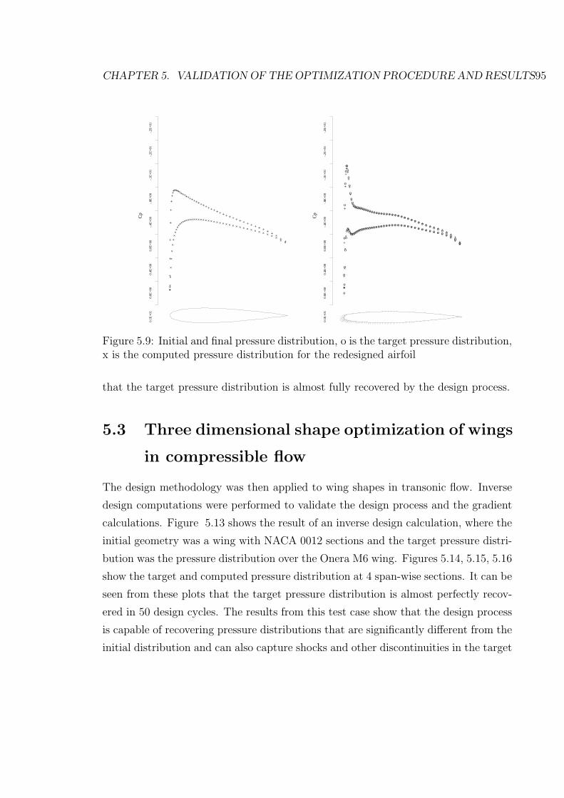
CHAPTER 5. VALIDATION OF THE OPTIMIZATION PROCEDURE AND RESULTS95
NACA 0012 TO ONERA MACH 0.000 ALPHA 1.796
CL 0.2117 CD 0.0041 CM -0.0029
GRID 160X32 NDES 0 RES0.469E-03 GMAX 0.100E-05
0.1E
+01
0.8E
+00
0.4E
+00
0.0E
+00
-.4E
+00
-.8E
+00
-.1E
+01
-.2E
+01
-.2E
+01
Cp
+++++++++++++++++++++++++++++++++++++++
++++
+
+
+
+
+++
+
+
+
+
+
+
+++++++++++++++++++++++++++ + + + + + + + + + + + + + + + +
++
NACA 0012 TO ONERA MACH 0.000 ALPHA 2.015
CL 0.2116 CD 0.0059 CM -0.0053
GRID 160X32 NDES 90 RES0.195E-04 GMAX 0.161E-04
0.1E
+01
0.8E
+00
0.4E
+00
0.0E
+00
-.4E
+00
-.8E
+00
-.1E
+01
-.2E
+01
-.2E
+01
Cp
++
++++++++++++++++++++++++++++++++++++++++++
+
+
+
+++
+
+
+
+
++++
+
+
+++++++++++++++++++++++ + + + + + + + + + + + + + + +
++
+oo
oooooooooooooooooooooooooooooooooooooooooo
o
o
o
o
o
o
o
o
o
oooo
o
o
oooooooooooooooooooo o o o o o o o o o o o o o o o o o o
oo
o
Figure 5.9: Initial and final pressure distribution, o is the target pressure distribution,x is the computed pressure distribution for the redesigned airfoil
that the target pressure distribution is almost fully recovered by the design process.
5.3 Three dimensional shape optimization of wings
in compressible flow
The design methodology was then applied to wing shapes in transonic flow. Inverse
design computations were performed to validate the design process and the gradient
calculations. Figure 5.13 shows the result of an inverse design calculation, where the
initial geometry was a wing with NACA 0012 sections and the target pressure distri-
bution was the pressure distribution over the Onera M6 wing. Figures 5.14, 5.15, 5.16
show the target and computed pressure distribution at 4 span-wise sections. It can be
seen from these plots that the target pressure distribution is almost perfectly recov-
ered in 50 design cycles. The results from this test case show that the design process
is capable of recovering pressure distributions that are significantly different from the
initial distribution and can also capture shocks and other discontinuities in the target
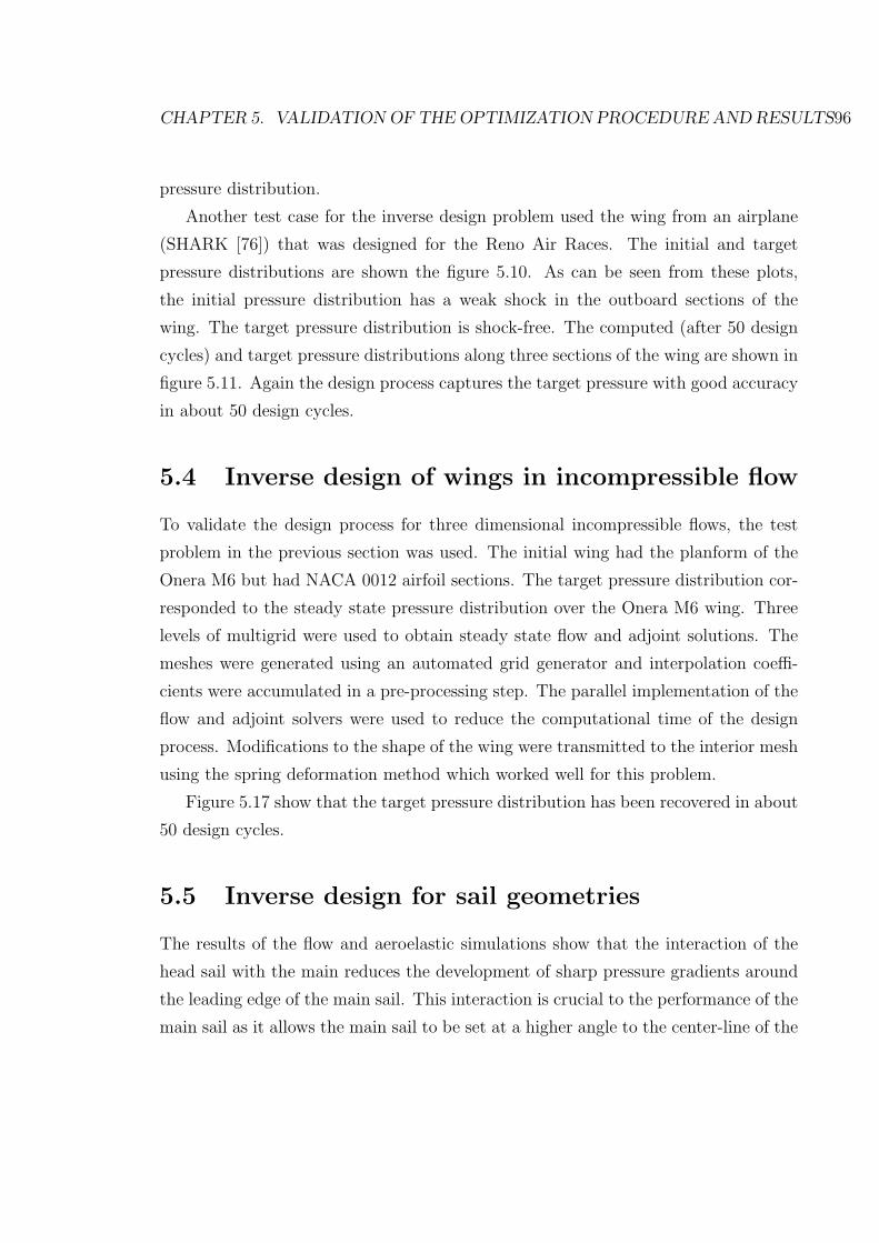
CHAPTER 5. VALIDATION OF THE OPTIMIZATION PROCEDURE AND RESULTS96
pressure distribution.
Another test case for the inverse design problem used the wing from an airplane
(SHARK [76]) that was designed for the Reno Air Races. The initial and target
pressure distributions are shown the figure 5.10. As can be seen from these plots,
the initial pressure distribution has a weak shock in the outboard sections of the
wing. The target pressure distribution is shock-free. The computed (after 50 design
cycles) and target pressure distributions along three sections of the wing are shown in
figure 5.11. Again the design process captures the target pressure with good accuracy
in about 50 design cycles.
5.4 Inverse design of wings in incompressible flow
To validate the design process for three dimensional incompressible flows, the test
problem in the previous section was used. The initial wing had the planform of the
Onera M6 but had NACA 0012 airfoil sections. The target pressure distribution cor-
responded to the steady state pressure distribution over the Onera M6 wing. Three
levels of multigrid were used to obtain steady state flow and adjoint solutions. The
meshes were generated using an automated grid generator and interpolation coeffi-
cients were accumulated in a pre-processing step. The parallel implementation of the
flow and adjoint solvers were used to reduce the computational time of the design
process. Modifications to the shape of the wing were transmitted to the interior mesh
using the spring deformation method which worked well for this problem.
Figure 5.17 show that the target pressure distribution has been recovered in about
50 design cycles.
5.5 Inverse design for sail geometries
The results of the flow and aeroelastic simulations show that the interaction of the
head sail with the main reduces the development of sharp pressure gradients around
the leading edge of the main sail. This interaction is crucial to the performance of the
main sail as it allows the main sail to be set at a higher angle to the center-line of the
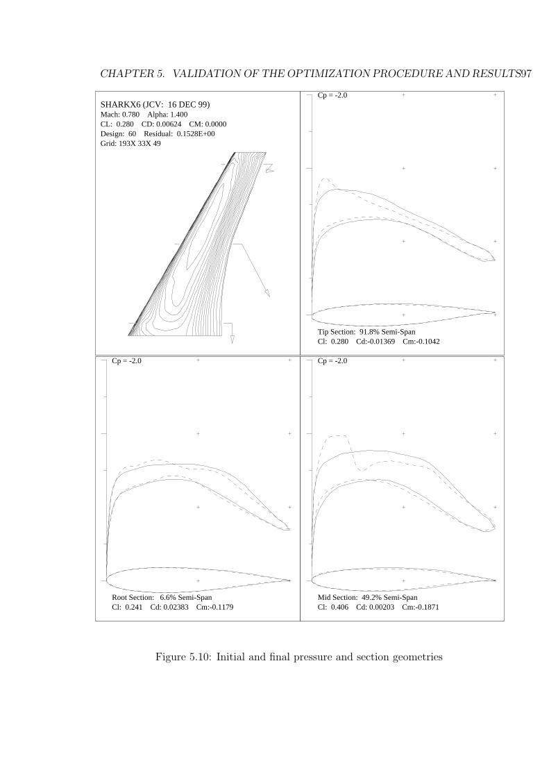
CHAPTER 5. VALIDATION OF THE OPTIMIZATION PROCEDURE AND RESULTS97
SHARKX6 (JCV: 16 DEC 99) Mach: 0.780 Alpha: 1.400 CL: 0.280 CD: 0.00624 CM: 0.0000 Design: 60 Residual: 0.1528E+00 Grid: 193X 33X 49
Cl: 0.241 Cd: 0.02383 Cm:-0.1179 Root Section: 6.6% Semi-Span
Cp = -2.0
Cl: 0.406 Cd: 0.00203 Cm:-0.1871 Mid Section: 49.2% Semi-Span
Cp = -2.0
Cl: 0.280 Cd:-0.01369 Cm:-0.1042 Tip Section: 91.8% Semi-Span
Cp = -2.0
Figure 5.10: Initial and final pressure and section geometries
CHAPTER 5. VALIDATION OF THE OPTIMIZATION PROCEDURE AND RESULTS98
SHARKX6 (JCV: 16 DEC 99) MACH 0.780 ALPHA 1.400 Z 16.548
CL 0.2787 CD 0.0120 CM -0.1352
GRID 192X32 NCYC 80 RES0.683E-03
0.1E
+01
0.8E
+00
0.4E
+00
0.3E
-07
-.4E
+00
-.8E
+00
-.1E
+01
-.2E
+01
-.2E
+01
Cp
++++
++
++
++
++
++
++++++++++++++++++++++++++++++++++++++++
++
+
+
+
+++
+
+
+
+
++++++++
+++++
++++
++++++++++++++++++++++++ + + +
++
++
++
++
++
++ooooo
oo
oo
oo
oo
oo
ooooooooooooooooooooooooooooooooooooooooooo
o
oooo
o
o
o
ooooooooooooo
oooo
ooooooooooooooooooo o o o o o o o o
oo
oo
oo
oo
oo
o
SHARKX6 (JCV: 16 DEC 99) MACH 0.780 ALPHA 1.400 Z 66.191
CL 0.4341 CD 0.0018 CM -0.2010
GRID 192X32 NCYC 80 RES0.683E-03
0.1E
+01
0.8E
+00
0.4E
+00
0.3E
-07
-.4E
+00
-.8E
+00
-.1E
+01
-.2E
+01
-.2E
+01
Cp
+++++++
++
++
++
++++++++++++++++++++++++++++++++++++++++++++
+
+
+++
+
+
+
+
+++++++++++++
+++++++
+++++++++++++++++++++ + ++
++
++
++
++
++
+
+ooooooo
oo
oo
oo
ooooooooooooooooooooooooooooooooooooooooooo
o
oooo
o
o
o
o
o
oooooooooooo
oooooo
oooooooooooooooooo o o o o o oo
oo
oo
oo
oo
oo
oo
SHARKX6 (JCV: 16 DEC 99) MACH 0.780 ALPHA 1.400 Z 115.834
CL 0.3122 CD -0.0139 CM -0.1244
GRID 192X32 NCYC 80 RES0.683E-03
0.1E
+01
0.8E
+00
0.4E
+00
0.3E
-07
-.4E
+00
-.8E
+00
-.1E
+01
-.2E
+01
-.2E
+01
Cp
++++++++
++++++++++++++++++++++++++++++++++++++++++++
++++
+
+
+
+++
+
+
+
+
+
+++++++++++
+++++++++++++++++++++++++++++ + + + + + + ++
++ + +
++
+ooooooo
oo
ooooooooooooooooooooooooooooooooooooooooo
oooooo
o
oooo
o
o
o
o
o
o
ooooooooooo
oooooooooooooooooooooooo o o o o o o o o o o oo
oo
o oo
oo
Figure 5.11: Initial and final pressure distributions at 5 %, 50 % and 95 % of thewing span

CHAPTER 5. VALIDATION OF THE OPTIMIZATION PROCEDURE AND RESULTS99
NACA 0012 WING TO ONERA M6 TARGET Mach: 0.840 Alpha: 3.060 CL: 0.325 CD: 0.02319 CM: 0.0000 Design: 0 Residual: 0.2763E-02 Grid: 193X 33X 33
Cl: 0.308 Cd: 0.04594 Cm:-0.1176 Root Section: 9.8% Semi-Span
Cp = -2.0
Cl: 0.348 Cd: 0.01749 Cm:-0.0971 Mid Section: 48.8% Semi-Span
Cp = -2.0
Cl: 0.262 Cd:-0.00437 Cm:-0.0473 Tip Section: 87.8% Semi-Span
Cp = -2.0
Figure 5.12: Initial pressure distribution over a NACA 0012 wing
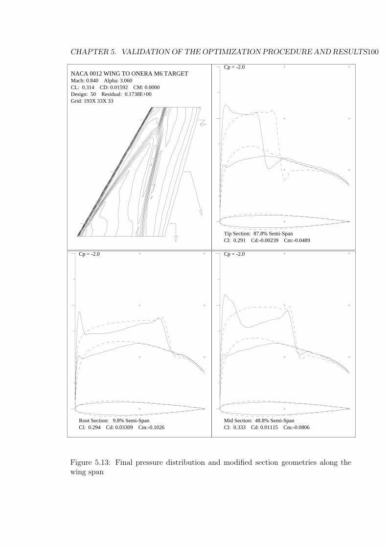
CHAPTER 5. VALIDATION OF THE OPTIMIZATION PROCEDURE AND RESULTS100
NACA 0012 WING TO ONERA M6 TARGET Mach: 0.840 Alpha: 3.060 CL: 0.314 CD: 0.01592 CM: 0.0000 Design: 50 Residual: 0.1738E+00 Grid: 193X 33X 33
Cl: 0.294 Cd: 0.03309 Cm:-0.1026 Root Section: 9.8% Semi-Span
Cp = -2.0
Cl: 0.333 Cd: 0.01115 Cm:-0.0806 Mid Section: 48.8% Semi-Span
Cp = -2.0
Cl: 0.291 Cd:-0.00239 Cm:-0.0489 Tip Section: 87.8% Semi-Span
Cp = -2.0
Figure 5.13: Final pressure distribution and modified section geometries along thewing span

CHAPTER 5. VALIDATION OF THE OPTIMIZATION PROCEDURE AND RESULTS101
NACA 0012 WING TO ONERA M6 TARGET MACH 0.840 ALPHA 3.060 Z 0.00
CL 0.2814 CD 0.0482 CM -0.1113
GRID 192X32 NDES 50 RES0.162E-02
0.1E
+01
0.8E
+00
0.4E
+00
0.3E
-07
-.4E
+00
-.8E
+00
-.1E
+01
-.2E
+01
-.2E
+01
Cp
++
++++++++++++++++++++++++++++++++++++++++++++++++++++
++++
+
+
+
++
++++
+
+
+
+
+
+
+
++
+
+
++++
+++++
++++++++++++++++++++++++++++++
+ ++
+
++ + +
++
++
+oo
oo
oooooooooooooooooooooooooooooooooooooooooooooooooooooo
o
o
o
o
oooo
o
o
o
o
o
o
oooo
o
oooo
ooooo
ooooooooooooooooooooooooo o o o o o
o oo
o
oo o o o
oo
oo
Figure 5.14: Final computed and target pressure distributions at 0 % and 20 %of thewing span
NACA 0012 WING TO ONERA M6 TARGET MACH 0.840 ALPHA 3.060 Z 0.40
CL 0.3269 CD 0.0145 CM -0.0865
GRID 192X32 NDES 50 RES0.162E-02
0.1E
+01
0.8E
+00
0.4E
+00
0.3E
-07
-.4E
+00
-.8E
+00
-.1E
+01
-.2E
+01
-.2E
+01
Cp
++
++
++++++++++++++++++++++++++++++++++++++++++++++++++++
++
+
+
+
+
+++
+
+
+
+
+
+
+
+
+
+
+++++++
++
+
+
+++++++++++++++++++++++++
++
+
+
+
+ ++ + + + + + + +
++
++o
oo
oooooooooooooooooooooooooooooooooooooooooooooooooo
ooooo
o
o
o
o
oooo
o
o
o
o
o
o
o
o
ooooooo
ooooooooooooooooooooooooooooo
oo
o
o
o
o o o o o o o o o oo
oo
o
NACA 0012 WING TO ONERA M6 TARGET MACH 0.840 ALPHA 3.060 Z 0.60
CL 0.3356 CD 0.0081 CM -0.0735
GRID 192X32 NDES 50 RES0.162E-02
0.1E
+01
0.8E
+00
0.4E
+00
0.3E
-07
-.4E
+00
-.8E
+00
-.1E
+01
-.2E
+01
-.2E
+01
Cp
++
++
++++++++++++++++++++++++++++++++++++++++++++++++++++
++
+
+
+
+
+++
+
+
+
+
+
+
+
+
+
+
+++++++++++++++
++++++++++++++++++
+++
+
+
++++ + + + + + + + + +
++
++o
oo
ooooooooooooooooooooooooooooooooooooooooooooooooooo
oooo
o
o
o
o
oooo
o
o
o
o
o
o
o
o
ooooooooooooooo
oooooooooooooooooo
ooo
o
o
o oo o o o o o o o o o o
oo
oo
Figure 5.15: Final computed and target pressure distributions at 40 % and 60 % ofthe wing span

CHAPTER 5. VALIDATION OF THE OPTIMIZATION PROCEDURE AND RESULTS102
NACA 0012 WING TO ONERA M6 TARGET MACH 0.840 ALPHA 3.060 Z 0.80
CL 0.3176 CD 0.0011 CM -0.0547
GRID 192X32 NDES 50 RES0.162E-02
0.1E
+01
0.8E
+00
0.4E
+00
0.3E
-07
-.4E
+00
-.8E
+00
-.1E
+01
-.2E
+01
-.2E
+01
Cp
++
+++++++++++++++++++++++++++++++++++++++++++++++++++++++
+
+
+
+
+
+++
+
+
+
+
+
+
+
+
+
++++++++++++++++++++++++
+++++
+
+
+
+
+
+++
++++++ + + + + + + + + +
++
++o
oo
ooooooooooooooooooooooooooooooooooooooooooooooooooo
oooo
o
o
o
o
oooo
o
o
o
o
o
o
o
o
oooooooooooooooooooooo
oooooo
o
o
o
o
o
ooo
o o o o o o o o o o o o o o oo
oo
o
NACA 0012 WING TO ONERA M6 TARGET MACH 0.840 ALPHA 3.060 Z 1.00
CL 0.4846 CD 0.0178 CM -0.1518
GRID 192X32 NDES 50 RES0.162E-02
0.1E
+01
0.8E
+00
0.4E
+00
0.3E
-07
-.4E
+00
-.8E
+00
-.1E
+01
-.2E
+01
-.2E
+01
Cp
+++++++++++++++++++++++++++++++++++++++++++++++++++++++++
+
+
+
+
++++
++
+
+
+
+
+
+
+
+++++++++++++++++++++++
+
+
+
+
++
++
++++++++++++ + + + + + + + + + ++ +
+ooooooooooooooooooooooooooooooooooooooooooooooooooooooooooo
o
o
o
ooo
o
o
o
o
o
o
o
o
o
oooooooooooooooooooooo
o
o
o
o
ooo
oooooooo o o o o o o o o o o o o o o o
oo
o
Figure 5.16: Final computed and target pressure distributions at 80 % and 100 % ofthe wing span
boat. These results also show that the region above the head sail has large suction
peaks which is a cause of concern. The aerodynamic shape optimization procedure
validated in the previous sections was used to redesign the main sail, with an aim of
reducing the pressure gradient around the luff of the main sail.
The cost function was defined as follows
I =
∫
B
(p− pt)2dB,
where p is the pressure distribution at the beginning of each design cycle, pt is the
pressure distribution obtained by smoothing the pressure distribution on the main
sail obtained from the aeroelastic analysis and the integral is taken over the surface
of the main sail. The lift was constrained by perturbing the angle of attack.
Figure 5.18 show that a significant portion of the leading edge of the main sail
has been redesigned to allow for smooth entry of the flow. The associated reduction
in sharp suction peaks should have a favorable affect on the growth of the boundary
layer over the upper surface. The change to the sections is shown in figure 5.19.

CHAPTER 5. VALIDATION OF THE OPTIMIZATION PROCEDURE AND RESULTS103
NACA 0012 TO ONERA M6 ALPHA 3.060 Z 0.000
CL 0.1890 CD 0.0186 CM -0.0594
NCYC 10 RES0.194E-02 DESIGN CYCLE 50
0.1E
+01
0.5E
+00
0.0E
+00
-.5E
+00
-.1E
+01
-.2E
+01
-.2E
+01
Cp
+o+o
+o+o+o+o+o+o+o+o+o+o+o+o+o+o+o+o+o+o+o+o+o+o+o+o+o+o+o+o+o+o+o+o+o+o+o+o+o+o+o+o+o+o+o+o+o+o+o+o+o+o+
o
+
o
+
o
+
o
+
o
+
o
+o
+o
+o+o
+o
+o
+o
+o
+o+o+o+o+o+o+o+o+o+o+o+o+o+o+o+o+o+o+o+o+o+o+o+o+o+o+o+o
+o+o+o+o+o+o+o+o+o+o+o+o+o+o+o+o+o+o +o +o +o +o +o +o +o +o+o
+o
NACA 0012 TO ONERA M6 ALPHA 3.060 Z 0.250
CL 0.2089 CD 0.0063 CM -0.0543
NCYC 10 RES0.194E-02 DESIGN CYCLE 50
0.1E
+01
0.5E
+00
0.0E
+00
-.5E
+00
-.1E
+01
-.2E
+01
-.2E
+01
Cp
+o+o+o+o+o+o+o+o+o+o+o+o+o+o+o+o+o+o+o+o+o+o+o+o+o+o+o+o+o+o+o+o+o+o+o+o+o+o+o+o+o+o+o+o+o+o+o+o+o+o+o+
o
+
o
+
o
+
o
+
o
+
o
+
o
+
o
+
o+o
+
o
+
o
+
o
+
o
+
o
+
o
+o
+o+o+o+o+o+o+o+o+o+o+o+o+o+o+o+o+o+o+o+o+o+o+o+o+o+o+o+o+o+o+o+o+o+o+o+o+o+o+o+o+o+o+o+o +o +o +o +o +o +o +o +o +o
+o
NACA 0012 TO ONERA M6 ALPHA 3.060 Z 0.750
CL 0.2299 CD 0.0032 CM -0.0573
NCYC 10 RES0.194E-02 DESIGN CYCLE 50
0.1E
+01
0.5E
+00
0.0E
+00
-.5E
+00
-.1E
+01
-.2E
+01
-.2E
+01
Cp
+o+o+o
+o+o+o+o+o+o+o+o+o+o+o+o+o+o+o+o+o+o+o+o+o+o+o+o+o+o+o+o+o+o+o+o+o+o+o+o+o+o+o+o+o+o+o+o+o+o+o+o+o+o
+
o
+
o
+
o
+
o
+
o
+
o
+
o
+o+
o
+
o
+
o
+
o
+
o
+
o
+
o
+o
+o+o+o
+o
+o
+o+o+o+o+o+o+o+o+o+o+o+o+o+o+o+o+o+o+o+o+o+o+o+o+o+o+o+o+o+o+o+o+o+o+o+o+o+o +o +o +o +o +o +o +o +o +o
+o
NACA 0012 TO ONERA M6 ALPHA 3.060 Z 1.000
CL 0.3340 CD 0.0219 CM -0.1151
NCYC 10 RES0.194E-02 DESIGN CYCLE 50
0.1E
+01
0.5E
+00
0.0E
+00
-.5E
+00
-.1E
+01
-.2E
+01
-.2E
+01
Cp
+o+o+o+o+o+o+o+o+o+o+o+o+o+o+o+o+o+o+o+o+o+o+o+o+o+o+o+o+o+o+o+o+o+o+o+o+o+o+o+o+o+o+o+o+o+o+o+o+o+o+o
+
o
+
o
+
o
+
o
+
o
+
o
+
o
+
o
+
o+
o
+
o
+
o
+
o
+
o
+
o
+
o
+
o
+
o
+o+o+o+o
+o
+o+o+o+o+o+o+o+o+o+o+o+o+o+o+o+o+o+o+o+o+o+o+o+o+o+o+o+o+o+o+o+o+o+o+o+o+o+o +o +o +o +o +o +o +o +o +o
+o
Figure 5.17: Final computed and target pressure distributions at 0, 25, 75 and 100 %of the wing span at 3 degrees angle of attack

CHAPTER 5. VALIDATION OF THE OPTIMIZATION PROCEDURE AND RESULTS104
The shape changes induced by the design method can be realized on an actual sail
by using battens. As the majority of the shape changes are induced near the leading
edge of the main sail, it is important to account for the presence of the mast to ensure
that the new shape provides favorable pressure gradients to the boundary layer.

CHAPTER 5. VALIDATION OF THE OPTIMIZATION PROCEDURE AND RESULTS105
TNZ : INVERSE DESIGN ALPHA 19.000 Z 4.975
CL 0.7850 CD 0.2799 CM -0.4489
NCYC 30 RES0.144E-02 DESIGN CYCLE 20
0.1E
+01
0.5E
+00
0.0E
+00
-.5E
+00
-.1E
+01
-.2E
+01
-.2E
+01
Cp
+o+o
+o+o+o+o+o+o+o+o+o+o+o+o+o+o+o+o+o+o+o+o+o+o+o+o+o+o+o+o+o+o+o+o+o+o+o+o+o
+
o
+o
+
o+
o
+
o
+o+o
+o+o
+o+o
+o
+o
+o
+o
+o
+o
+o
+o+o+o+o+o+o+o+o+o+o+o+o+o+o+o+o+o+o+
o+o+
o+o+o
+o
TNZ : INVERSE DESIGN ALPHA 19.000 Z 10.981
CL 0.9992 CD 0.2965 CM -0.5381
NCYC 30 RES0.144E-02 DESIGN CYCLE 20
0.1E
+01
0.5E
+00
0.0E
+00
-.5E
+00
-.1E
+01
-.2E
+01
-.2E
+01
Cp
+o
+o
+o
+o
+o
+o
+o
+o
+o
+o
+o
+o
+o
+o+o+o+o+o+o+o+o+o+o+o
+o
+o
+o
+o
+o
+o
+o
+o
+o
+o
+o
+o+o+o+
o+
o
+
o
+
o
+
o
+
o
+
o+o+o
+o
+o
+
o
+
o
+
o
+
o
+
o
+
o
+
o
+
o
+o
+o+o+o+o+o+o+o+o+o+o+o+o+o+o+o+
o+o+
o+o+
o+o+o+o
TNZ : INVERSE DESIGN ALPHA 19.000 Z 23.366
CL 1.4461 CD 0.2735 CM -0.6545
NCYC 30 RES0.144E-02 DESIGN CYCLE 20
0.1E
+01
0.5E
+00
0.0E
+00
-.5E
+00
-.1E
+01
-.2E
+01
-.2E
+01
Cp
+o+o
+o+o
+o+o+o+o+o+o+o+o+o+o+o
+o
+o
+o
+o
+o
+o
+o
+o
+o
+
o
+
o
+
o
+
o
+
o
+
o
+
o
+
o
+
o
+
o+o
+o
+o+
o+
o
+
o
+o
+
o
+
o
+
o
+
o
+o+
o
+
o
+
o
+
o
+
o
+
o
+
o
+
o
+
o
+
o
+
o
+
o
+
o
+
o
+
o
+
o
+
o+
o+o+
o+o+o+o+o+o+o
+o+o+o
+o+o+o+o+o+o
TNZ : INVERSE DESIGN ALPHA 19.000 Z 26.494
CL 1.5637 CD 0.2928 CM -0.6885
NCYC 30 RES0.144E-02 DESIGN CYCLE 20
0.1E
+01
0.5E
+00
0.0E
+00
-.5E
+00
-.1E
+01
-.2E
+01
-.2E
+01
Cp
+o
+o+o+o
+o+o+o+o+o+o+o+o+
o+o
+o
+o
+o
+o
+o
+o
+o
+o
+o
+o
+
o
+
o
+
o
+
o
+
o
+
o
+
o
+
o
+
o
+
o
+
o+o
+o+
o+
o
+
o
+
o
+
o
+
o
+
o
+
o
+o+o
+
o
+
o
+
o
+
o
+
o
+
o
+
o
+
o
+
o
+
o
+
o
+
o
+
o
+
o
+
o
+
o+
o+o+o+
o+o+o+o+
o+o+o+o+o+o+o+o+o+o+o
Figure 5.18: Initial (o) and final(+,x) pressure distribution at 15, 32, 75 and 85%height on the main sail

CHAPTER 5. VALIDATION OF THE OPTIMIZATION PROCEDURE AND RESULTS106
11 12 13 14 15 16 17 18 19−3
−2
−1
0
1
2
3
Initial and deformed sections at 15 percent height
x
y
InitialRedesign
11 12 13 14 15 16 17 18
−2
−1
0
1
2
3
Initial and deformed sections at 32 percent height
x
y
InitialRedesign
11 12 13 14 15 16 17
−2
−1.5
−1
−0.5
0
0.5
1
1.5
2
2.5
3
Initial and deformed sections at 75 percent height
x
y
InitialRedesign
11.5 12 12.5 13 13.5 14 14.5 15 15.5 16 16.5
−1.5
−1
−0.5
0
0.5
1
1.5
2
2.5
Initial and deformed sections at 85 percent height
x
y
InitialRedesign
Figure 5.19: Initial and redesigned camber line at 15,32,75 and 85% of height
Chapter 6
Conclusions
6.0.1 Aerodynamic and Aeroelastic analysis
The use of robust and accurate numerical methods for the Euler equations along
with the use of parallel computing environments enable designers to characterize the
aerodynamic performance of the design. Due to the fast turn-around times of these
simulations it will now be possible to substitute potential flow solvers with these non-
linear models of the flow field, thereby obtaining improved estimates of the forces on
sail configurations. As the computational tools that were developed in this study were
based on unstructured grids, including the other components of the sail-boat into the
analysis procedure will be straight-forward. Hence it is reasonable to expect that the
analysis tools developed in this study can be used as building blocks to develop an
integrated computational tool to determine the forces and moments generated during
the motion of the boat.
An obvious extension to the analysis tools developed in this study is the need to
include viscous effects in the mathematical models. Numerical solutions to the RANS
equations should be the goal. Computational tools that solve the RANS equations
are quite popular within the CFD community. However, it requires a trained user
to extract the quantities of engineering interest from these simulations. The first
major hurdle is encountered during the grid generation phase. Turbulence models
could potentially pose another hurdle. As an intermediate step, it is conceivable
107

CHAPTER 6. CONCLUSIONS 108
that inviscid flow solvers coupled with boundary layer codes could alleviate some of
the difficulties. The fast turn-around times of these simulations could provide an
attractive alternative to the designer.
The results of the aeroelastic simulations confirm that the elastic nature of the sail
cloth could play an important role in the aerodynamic performance of a design. The
techniques used in this study take first step towards building an integrated aeroelastic
package. To provide accurate estimates of the flying shape it will be necessary to
develop an improved structural analysis code that takes into account the various
elements of the rigs, wrinkling, flexibility of the mast, and presence of the battens.
The appropriate choice of finite element discretization procedures is also an open
question that needs to be addressed in the future.
6.0.2 Aerodynamic design
While analysis tools (aerodynamic and aeroelastic) can provide the designer with
insights into the performance of the design, an automated design tool that arrives at
the optimum design is invaluable. This study has confirmed the feasibility of adjoint
based shape optimization procedures for determining the optimal shape of the sail
sections. As the changes made by the design procedure are small and localized,
alternate design methods would have to perform iterative analysis of a large number
of candidate designs. Hence, the adjoint design method can provide a unique tool for
sail designers.
The multi-disciplinary nature of the design process for sailboats is illustrated in
figure 6.1. This flow chart (from [77]) shows the interaction of the various forces and
moments that result in a particular speed-made good (Vmg) of a design. The develop-
ment of an integrated computational tool to optimize the windward performance of
the boat is clearly feasible. As part of the current research some of the building blocks
for this computational tool have been developed. However they require refinement
and improvement, and this will be the task for the future.
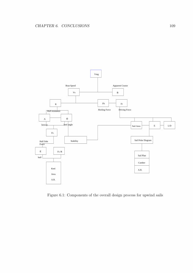
CHAPTER 6. CONCLUSIONS 109
L/DSail Area
Keel
Area
hull
Fs /RΕ
A.R.
E
Sail Polar Diagram
A.R.
Camber
Sail Plan
Hull Side
Fr
Vs
Vmg
Β
Driving ForceHeeling Force
Apparent CourseBoat Speed
Fh
heel angle
Stability
Fs
Force
leeway
R
Hull resistance
ΘΛ
Figure 6.1: Components of the overall design process for upwind sails
Bibliography
[1] S. Collie, M. Gerritsen and P. Jackson, A Review of Turbulence Modeling for
Use in Sail Flow Analysis School of Engineering Report, No. 603, University of
Auckland, New Zealand.
[2] T. Doyle, M. Gerritsen and G. Iaccarino, Optimization of Yard Sectional Shape
and Configuration of a Modern Clipper Ship, Proceedings of the 17th International
HISWA Symposium of Yacht Design and Yacht Construction, November, 2002.
[3] A. Rizzi and L. Eriksson, Computation of inviscid incomrpessible flow with rota-
tion, Journal of Fluid Mechanics Vol. 153, pp 275-312, 1985.
[4] P. M. Gresho, Incompressible Fluid Dynamics: Some Fundamental Formulation
Issues, Annual Review of Fluid Mechanics, Vol. 23, pp 413-453, 1991.
[5] T. Charvet and S. G Huberson, Numerical Calculation of the flow around sails,
European Journal of Mechanics, Vol. 11, Part B. Fluids, pp 599-610, 1992.
[6] P. S. Jackson and G. W. Christie, Numerical analysis of three dimensional elastic
membrane wings AIAA Journal, Vol. 25, 5, pp 676-682, 1986.
[7] T. Fukusawa and M. Katori, Numerical approach to aeroelastic responses of three
dimensional flexible sails. The Eleventh Chesapeake Sailing Yacht Symposium,
1993.
[8] R. K. Miller and J. M. Hedgepeth, An Algorithm for Finite Element Analysis of
Partly Wrinkled Membranes, AIAA Journal, Technical Note 82-4293, pp 1761-
1763, 1982.
110

BIBLIOGRAPHY 111
[9] M. Stein and J. M. Hedgepeth, Analysis of Partially wrinkled membranes, NASA
Technical Note TN D-813, July 1961.
[10] J. H. Milgram, Sail Force Coefficients for systematic Rig Variations, SNAME
Technical and Research Report R-10, 1971.
[11] J. H. Milgram, Analytic Design of sail yachts, Transactions of SNAME Vol. 76,
pp 118-160, 1968.
[12] J. H. Milgram, Effects of Masts on the Aerodynamics of Sail sections, Marine
Technology Vol. 15, No. 1, pp. 35-42, 1978.
[13] Burns Fallow, Private Communication.
[14] J. H. Milgram, The analysis of three dimensional Sails, Proceedings of the 10th
Canadian Congress of Applied Mechanics University of Western Ontario, London,
Canada, pp 59-67, 1985.
[15] T. Sugimoto, A method for optimizing sail design, Sports Engineering Vol. 2,
pp 35-48, 1999.
[16] A. H. Day, The optimisation of aerodynamic lift distribution for a heeled yacht
in a wind gradient, Transactions of the Royal Institution of Naval Architects, 134,
91-108, 1994.
[17] T. Sugimoto, A first course in optimum design of yacht sails, Fluid Dynamics
Research Vol.11, 1993.
[18] N. J. Locke, P. S. Jackson and R. G. J. Flay, Lift and drag distributions of yacht
sails using wake surveys, Journal of Fluids engineering Vol.118, 1996.
[19] R. G. J. Flay and P. S. Jackson, Flow simulation for wind tunnel studies of
sail aerodynamics, Journal of Wind Engineering and Industrial Aerodynamics
Vol.41-44, 1992.
[20] J. G. Ladesic and R .K. Irey, An experimental investigation of yacht sail aero-
dynamics, AIAA monographs Vol.29, 1983.

BIBLIOGRAPHY 112
[21] P. Atkinson and J. A. Szantyr, An integrated approach to the analysis of mast-
sail systems, Proceedings of RINA 1991.
[22] P. Atkinson, On the structural response of a mast sail system, International
conference on Computer Aided Design for Small Craft - Sail and Power Vol.1,
1988.
[23] J. N. Selness, The finite element method of structural analysis applied to mast
rigs, The 10th AIAA Symposium of Sailing, The Ancient Interface X, Vol. 26,
1990.
[24] F. Muttin, Structural analysis of sails, European Journal of Mechanics A/Solids,
Vol. 10, 5, pp. 517-534, 1990.
[25] H. Schoop, Structural and Aerodynamic theory for sails, European Journal of
Mechanics A/Solids, Vol. 9, 1, pp. 37-52, 1990.
[26] A. Jameson, Re-Engineering the Design Process through Computation, AIAA
Paper 97-0641, 35th AIAA Aerospace Sciences Meeting, Reno, January, 1997.
[27] J.J. Alonso, L. Marinelli, A. Jameson, Multigrid Unsteady Navier-Stokes Cal-
culations with Aeroelastic Applications, AIAA Paper 95-004, 33rd Aerospace
Sciences Meeting and Exhibit, Reno, NV, January 1995.
[28] A. Jameson and T.J. Baker, Improvements to the Aircraft Euler Method, AIAA
Paper 87-0353, 25th AIAA Aerospace Sciences Meeting, Reno, January, 1987.
[29] J. Ruether, A. Jameson, J. Farmer, L. Martinelli and D. Saunders, Aerodynamic
Shape optimization of complex aircraft configurations via an adjoint method,
AIAA Paper 96-0094, 34th AIAA Aerospace Sciences Meeting, Reno, January,
1996.
[30] A. Chorin, A Numerical Method for Solving the Incompressible Viscous Flow
problem, Journal of Computational Physics Vol. 2, pp 12-26, 1967.

BIBLIOGRAPHY 113
[31] J. Farmer, L. Martinelli and A. Jameson, A Fast Multigrid Method for Solving
Incompressible Hydrodynamic Problems with Free Surfaces, AIAA Paper 93-
0767, 31st AIAA Aerospace Sciences Meeting, Reno, January, 1993.
[32] A. Jameson, W. Schmidt and E. Turkel, Numerical Solution of the Euler equa-
tions by finite volume methods using Runger-Kutta time stepping schemes, AIAA
Paper 81-1259, June, 1981.
[33] J. A. Dessideri and A. Derivieux, Compressible flow Solvers using unstructured
grids, VKI Lecture Series 1988-05, March 7-11, 1988.
[34] S. R. Allmaras and M. B. Giles, A second order Flux Split Scheme for the Un-
steady 2-D Euler Equations on Arbitrary meshes, AIAA Paper 87-1119, January
1987.
[35] T. J. Barth and D. C. Jesperson, The design and application of upwind schemes
on unstructured meshes, AIAA Paper 89-0366, January 1989.
[36] A. Jameson, Analysis and Design of numerical schemes for gas dynamics 2, artifi-
cial diffusion and discrete shock structure, International Journal of Computational
Fluid Dynamics, Vol. 5, pp. 1-38, 1995.
[37] A. Jameson, Multigrid algorithms for compressible flow calculations, Proceedings
of the 2nd European Conference on Multigrid Methods, Cologne, 1985.
[38] A. Jameson, Private Communication, unpublished notes.
[39] S.K. Kim, J.J. Alonso, A. Jameson, Two-Dimensional High-Lift Aero-
dynamic Optimization Using the Continuous Adjoint Method, 8th
AIAA/USAF/NASA/ISSMO Symposium on Multidisciplinary Analysis and Op-
timization, AIAA Paper 2000-4741, Long Beach, CA, September 2000.
[40] A. Jameson, Computational Aerodynamics for Aircraft Design, Science, Vol.
245, pp. 261-371, 1989.

BIBLIOGRAPHY 114
[41] A. Jameson, A Perspective on Computational Algorithms for Aerodynamic
Shape Analysis and Design, Progress in Aerospace Sciences, Elsvier, 2001.
[42] A. Jameson, Aerodynamic design via control theory, Journal of Scientific Com-
puting, 3:233–260, 1988.
[43] A. Jameson, Optimum aerodynamic design using CFD and control theory, AIAA
paper 95-1729, AIAA 12th Computational Fluid Dynamics Conference, San Diego,
CA, June 1995.
[44] J. Reuther, A. Jameson, J. Farmer, L. Martinelli, and D. Saunders, Aerody-
namic shape optimization of complex aircraft configurations via an adjoint for-
mulation, AIAA paper 96-0094, 34th Aerospace Sciences Meeting and Exhibit,
Reno, Nevada, January 1996.
[45] J. Reuther, J. J. Alonso, J. C. Vassberg, A. Jameson, and L. Martinelli, An
efficient multiblock method for aerodynamic analysis and design on distributed
memory systems, AIAA paper 97-1893, June 1997.
[46] J. J. Reuther, A. Jameson, J. J. Alonso, M. Rimlinger, and D. Saunders, Con-
strained multipoint aerodynamic shape optimization using an adjoint formulation
and parallel computers: Part I, Journal of Aircraft, 36(1):51–60, 1999.
[47] J. J. Reuther, A. Jameson, J. J. Alonso, M. Rimlinger, and D. Saunders, Con-
strained multipoint aerodynamic shape optimization using an adjoint formulation
and parallel computers: Part II, Journal of Aircraft, 36(1):61–74, 1999.
[48] J.L. Lions, Optimal Control of Systems Governed by Partial Differential Equa-
tions, Springer-Verlag, New York, 1971. Translated by S.K. Mitter.
[49] S. Nadarajah, A. Jameson, A Comparison of the Continuous and Discrete
Adjoint Approach to Automatic Aerodynamic Optimization, AIAA-2000-0667,
AIAA 38th Aerospace Sciences Meeting and Exhibit, Reno, NV, January 2000.
[50] O. Pironneau, Optimal Shape Design for Elliptic Systems, Springer-Verlag, New
York, 1984.

BIBLIOGRAPHY 115
[51] A. Jameson, Re-engineering the design process through computation, AIAA
paper 97-0641, 35th Aerospace Sciences Meeting and Exhibit, Reno, Nevada, Jan-
uary 1997.
[52] J. Reuther, J.J. Alonso, M.J. Rimlinger, and A. Jameson, Aerodynamic shape
optimization of supersonic aircraft configurations via an adjoint formulation on
parallel computers, AIAA paper 96-4045, 6th AIAA/NASA/ISSMO Symposium
on Multidisciplinary Analysis and Optimization, Bellevue, WA, September 1996.
[53] W. K. Anderson and V. Venkatakrishnan, Aerodynamic design optimization on
unstructured grids with a continuous adjoint formulation, AIAA paper 97-0643,
35th Aerospace Sciences Meeting and Exhibit, Reno, Nevada, January 1997.
[54] J. Reuther, A. Jameson, J. J. Alonso, M. J. Rimlinger, and D. Saunders, Con-
strained multipoint aerodynamic shape optimization using an adjoint formulation
and parallel computers, AIAA paper 97-0103, 35th Aerospace Sciences Meeting
and Exhibit, Reno, Nevada, January 1997.
[55] A. Jameson and J.C. Vassberg, Studies of alternative numerical optimization
methods applied to the brachistochrone problem, Computational Fluid Dynamics,
9:281–296, 2000.
[56] J. Elliott and J. Peraire, Aerodynamic design using unstructured meshes, AIAA
paper 96-1941, June 1997.
[57] Eric J. Nielson and W. Kyle Anderson, Aerodynamic design optimization on
unstructured meshes using the Navier-Stokes equations, AIAA Journal, 37:1411–
1419, 1998.
[58] J. Reuther, Aerodynamic shape optimization using control theory, Ph. D. Dis-
sertation, University of California, Davis, Davis, CA, June 1996.
[59] J. R. R. A. Martins, I. M. Kroo, and J. J. Alonso, An automated method
for sensitivity analysis using complex variables, AIAA paper 2000-0689, 38th
Aerospace Sciences Meeting, Reno, Nevada, January 2000.

BIBLIOGRAPHY 116
[60] C. Bischof, A. Carle, G. Corliss, A. Griewank, and P. Hovland, Generating
derivative codes from Fortran programs, Internal report MCS-P263-0991, Com-
puter Science Division, Argonne National Laboratory and Center of Research on
Parallel Computation, Rice University, 1991.
[61] A. Jameson, N. Pierce, and L. Martinelli, Optimum aerodynamic design using the
Navier-Stokes equations, AIAA paper 97-0101, 35th Aerospace Sciences Meeting
and Exhibit, Reno, Nevada, January 1997.
[62] A. Jameson, L. Martinelli, and N. A. Pierce, Optimum aerodynamic design using
the Navier-Stokes equations, Theoretical and Computational Fluid Dynamics,
10:213–237, 1998.
[63] A. Jameson, Automatic design of transonic airfoils to reduce the shock induced
pressure drag, In Proceedings of the 31st Israel Annual Conference on Aviation
and Aeronautics, Tel Aviv, pages 5–17, February 1990.
[64] A. Jameson, Optimum aerodynamic design via boundary control, In AGARD-
VKI Lecture Series, Optimum Design Methods in Aerodynamics. von Karman
Institute for Fluid Dynamics, 1994.
[65] W. Kyle Anderson and Dary L. Bonhaus, Navier-stokes computations and exper-
imental comparisons for multielement airfoil configurations, Journal of Aircraft,
32:1246–1253, 1993.
[66] J. Reuther, A. Jameson, J. Farmer, L. Martinelli, and D. Saunders, Aerodynamic
shape optimization of complex aircraft configurations via an adjoint formulation,
AIAA paper 96-0094, AIAA 34th Aerospace Sciences Meeting and Exhibit, Reno,
NV, January 1996.
[67] A. Jameson, Multigrid algorithms for compressible flow calculations, In W. Hack-
busch and U. Trottenberg, editors, Lecture Notes in Mathematics, Vol. 1228, pages
166–201. Proceedings of the 2nd European Conference on Multigrid Methods,
Cologne, 1985, Springer-Verlag, 1986.
BIBLIOGRAPHY 117
[68] A. Jameson, Steady state solution of the Euler equations for transonic flow,
In Proceedings of Symposium on Transonic, Shock, and Multidimensional Flows,
pages 30–37, Academic Press, New York, 1982.
[69] C. Hirsch, Numerical Computation of Internal and External Flows, volume 1,
John Wiley & Sons, New York, 1988.
[70] C. Hirsch, Numerical Computation of Internal and External Flows, volume 2,
John Wiley & Sons, New York, 1990.
[71] A. Jameson, Optimum Aerodynamic Design Using Control Theory, Computa-
tional Fluid Dynamics Review 1995 Wiley, 1995.
[72] A. Jameson, L. Martinelli and J. Vassberg, Using CFD for Aerodynamics - A
critical Assesment, Proceedings of ICAS 2002, September 8-13, 2002, Toronto,
Canada.
[73] A. Jameson, Sangho Kim, Reduction of the Adjoint Gradient Formula in the
Continuous Limit, AIAA Paper, 41st AIAA Aerospace Sciences Meeting, Reno
January, 2003.
[74] G. Cowles and Luigi Martinelli, A Control-Theory Based Method for Shape
Design in Incompressible Viscous Flow using RANS, AIAA Fluids 2000-2544,
June 19-22, Denver, CO.
[75] A. Jameson and Luigi Martinelli, Aerodynamic Shape Optimization Techniques
Based on Control Theory, CIME (International Mathematical Summer Center),
Martina Fran-ca, Italy, June 1999.
[76] E. Ahlstrom, R. Gregg, J. Vassberg, A. Jameson, G-Force: The design of an
unlimited Class Reno Racer, AIAA Paper, 18th AIAA Applied Aerodynamics
Conference, Denver August, 2000.
[77] C. A. Marchaj, Aerohydrodynamics of Sailing, Third Edition, Published by
Adlard Coles National, 2000.