Null Models of Economic Networks:

The Case of the World Trade Web

Giorgio Fagiolo∗ Tiziano Squartini† Diego Garlaschelli‡

December 2011

Abstract

In all empirical-network studies, the observed properties of economic networks are informativeonly if compared with a well-defined null model that can quantitatively predict the behaviorof such properties in constrained graphs. However, predictions of the available null-modelmethods can be derived analytically only under assumptions (e.g., sparseness of the network)that are unrealistic for most economic networks like the World Trade Web (WTW). In thispaper we study the evolution of the WTW using a recently-proposed family of null networkmodels. The method allows to analytically obtain the expected value of any network statisticacross the ensemble of networks that preserve on average some local properties, and areotherwise fully random. We compare expected and observed properties of the WTW in theperiod 1950-2000, when either the expected number of trade partners or total country trade iskept fixed and equal to observed quantities. We show that, in the binary WTW, node-degreesequences are sufficient to explain higher-order network properties such as disassortativityand clustering-degree correlation, especially in the last part of the sample. Conversely, in theweighted WTW, the observed sequence of total country imports and exports are not sufficientto predict higher-order patterns of the WTW. We discuss some important implications ofthese findings for international-trade models.

Keywords: World Trade Web; Null Models of Networks; Complex Networks; InternationalTrade.

JEL Classification: D85, C49, C63, F10.

∗Corresponding Author. Sant’Anna School of Advanced Studies, Pisa, Italy. Mail address: Sant’Anna School ofAdvanced Studies, Piazza Martiri della Liberta 33, I-56127 Pisa, Italy. Tel: +39-050-883282. Fax: +39-050-883344.Email: giorgio.fagiolo@sssup.it

†CSC and Department of Physics, University of Siena, Via Roma 56, 53100 Siena (Italy) and Instituut-Lorentzfor Theoretical Physics, Leiden Institute of Physics, University of Leiden, Niels Bohrweg 2, 2333 CA Leiden (TheNetherlands).

‡Instituut-Lorentz for Theoretical Physics, Leiden Institute of Physics, University of Leiden, Niels Bohrweg 2,2333 CA Leiden (The Netherlands).

1

1 Introduction

In the last years an increasing number of contributions have been addressing the study of economic

systems and their dynamics in terms of networks (Schweitzer et al., 2009). The description of an

economic system as a network requires to characterize economic units (e.g., countries, industries,

firms, consumers, individuals, etc.) as nodes and their market and non-market relationships as links

between them. Successive snapshots of these interacting structures can give us a clue about how

networked systems evolve in time. Heterogeneity of agent and link types can be easily considered.

Nodes can be tagged with different characteristics or properties (e.g., economic size) and links

may be defined to be directed or undirected, binary or weighted, etc., according to the focus of

the analysis.

The study of economic networks has recently proceeded along three main complementary di-

rections. First, a large body of empirical contributions have investigated the topological properties

of many real-world economic and social networks (Caldarelli, 2007), ranging from macroeconomic

networks where nodes are countries and linkages represent trade or financial transactions, all the

way to firm and consumer networks where links represent knowledge or information exchange.

This empirical-research program has generated a very rich statistical evidence, pointing to many

differences and similarities in the way economic networks are shaped. As a consequence, a very

fertile ground for theoretical work has emerged.

Second, a stream of theoretical research has explored efficiency properties of equilibrium net-

works arising in cooperative and non-cooperative game-theoretic setups, where players have the

possibility to choose both their strategy in the game and whom to play the game with (Goyal,

2007; Vega-Redondo, 2007; Jackson, 2008). Despite such models have been very successful in

highlighting the role of network structure in explaining aggregate outcomes, they fell short from

providing a framework where observed network regularities can be reproduced and explained.

Third, a large number of contributions rooted in the econophysics tradition1 have been devel-

oping simple stochastic models of network evolution where nodes hold very stylized and myopic

probabilistic rules determining their future connectivity patterns in the network (Newman, 2010).

The two foremost examples of such an approach are Watts and Strogatz (1998) small-world model

and Albert and Barabasi (2002) preferential-attachment model. Despite this family of stochas-

tic models are able to reproduce observed economic-network patterns, the extent to which such

stylized representations can be employed to understand causal relations between incentive-based

choices made in strategic contexts and the overall efficiency of the long-run equilibrium networks

is still under scrutiny.

All that hints to the dramatic need for theoretical models that are able to reproduce and eco-

nomically explain the observed patterns of topological properties in real-world networks. Despite

1For an introduction to econophysics, see Mantegna and Stanley (1999); Sinha et al. (2010). Cf also Rosser(2008a,b).

2

we know a great deal about how economic networks are shaped in reality and what that means

for dynamic processes going on over networked structures (e.g., diffusion of shocks and contagion

effects, cf. for example Allen and Gale, 2001; Battiston et al., 2009), we still lack a clear under-

standing of why real-world network architectures looks like they do, and how all that has to do

with individual incentives and social welfare.

This paper contributes to the aforementioned debate by exploring an alternative approach

to the trade-off between explanation and reproduction of topological properties, grounded in the

generation of null (random) network models. The idea is not new. Instead of building economically-

or stochastically-based micro-foundations for explaining observed patterns, one tries to ask the

question whether observed statistical-network properties may be simply reproduced by simple

processes of network generation that only match some (empirically-observed) constraints, but are

otherwise fully random. If they do, then the researcher may conclude that such regularities are not

that interesting from an economic point of view, as no alternative, more structural, model would

pass any test discriminating against the random counterpart. Conversely, if observed regularities

cannot be reproduced by the null random model, we are led to argue that some more structural

economic process may be responsible for what we observe. Null random-network models may

therefore serve as a sort of sieve that can help us to discriminate between interesting and useless

observed-network properties. Exactly as in statistics and econometrics one performs significance

tests, null network models are very helpful to understand the distributional properties of a given

network statistics, under very mild null hypotheses for the underlying network-generation process.2

Null (random) network models have been extensively used in the recent past (see Squartini and

Garlaschelli, 2011, for a review). Since the seminal work of Erdos and Renyi (1960) on random

graphs, many alternative null network models have been proposed.3 A useful way of classifying

them is according to the constraints they pose in the way the otherwise-random mechanism of

network construction works. A large number of contributions, for example, have been focussing

on generating random networks able to control (exactly or on average) for the degree sequence

in binary graphs, or for the strength sequence in weighted ones. This is reasonable, as degree

and strength sequences are one of the most basic statistics characterizing graphs. It is therefore

very important to study the properties of network statistics (other than degrees and strengths)

in ensembles of otherwise fully-random graphs preserving those basic topological quantities (and

thus looking somewhat similar to the observed one).

However, most of the existing network null-model methods suffer from important limitations. A

large class of algorithms generates randomized variants of a network computationally, through iter-

ated “moves” that locally rewire the original connections in such a way that the desired constraints

2In economics the use of purely-random models is not new. Examples range from industrial agglomeration(Ellison and Glaeser, 1997; Rysman and Greenstein, 2005) to international trade (Armenter and Koren, 2010).

3See for example Katz and Powell (1957); Holland and Leinhardt (1976); Snijders (1991); Rao et al. (1996);Kannan et al. (1999); Roberts (2000); Newman et al. (2001); Shen-Orr et al. (2002); Maslov et al. (2004); Ansmannand Lehnertz (2011); Bargigli and Gallegati (2011).

3

remain unchanged (Shen-Orr et al., 2002; Maslov and Sneppen, 2002; Maslov et al., 2004). These

approaches are extremely demanding in terms of computation time. In order to obtain expecta-

tions from the null model, one has indeed to constructively build many alternative random graphs

belonging to the desired family, then measure any target topological property on each of such

randomized graphs, and finally perform a final sample average of this property. At the opposite

extreme, analytical approaches have been proposed in order to obtain mathematical expressions

characterizing the expected properties, thus avoiding time-consuming randomizations (Newman

et al., 2001; Chung and Lu, 2002; Serrano and Boguna, 2005; Bargigli and Gallegati, 2011). The

problem with the latter approaches is that they are only valid under specific hypotheses about the

structure of the original network. For instance, methods based on probability generating functions

are generally only valid for sparse and locally tree-like (thus with vanishing clustering) networks

(Newman et al., 2001). Similarly, models predicting factorized connection probabilities in binary

graphs (Chung and Lu, 2002) or factorized expected weights in weighted networks (Serrano and

Boguna, 2005; Bargigli and Gallegati, 2011) make (either explicitly or implicitly) the assumption

of sparse networks, as has been shown recently (Squartini and Garlaschelli, 2011). Additionally,

each method or algorithm is generally designed to generate random networks satisfying a specific

set of constraints (e.g., degree sequence) and cannot be easily extended to cover different sets of

constraints (e.g., strength sequence, possibly in directed-graph contexts). For instance, a problem

that inherently pervades random models of weighted networks is the simplifying assumption of

real-valued edge weights (Bhattacharya et al., 2008; Ansmann and Lehnertz, 2011; Fronczak and

Fronczak, 2011). When made in models that specify the strength sequence, this assumption leads

to randomized ensembles of networks where edges with zero weight have zero probability, so that

the typical networks are fully connected (Ansmann and Lehnertz, 2011; Fronczak and Fronczak,

2011). This actually makes the original network an unlikely outcome of the model, rather than

one with the same probability as all other instances with the same sufficient statistics (e.g. with

the same strength sequence).

In this paper we employ a recently-proposed method that overcomes all the above restrictions

simultaneously (Squartini and Garlaschelli, 2011). The method is analytical and therefore does

not require simulations to generate the family of all randomized variants of the target network.

This important property makes the method very fast and strongly facilitates exhaustive analyses

which require the analysis of many networks, e.g. in order to track the temporal evolution of a

particular system or to study all the individual components of a multi-network with many layers, or

both (Squartini et al., 2011a,b). At the same time, the method does not make assumptions about

the structure of the original network, and therefore works also for dense and clustered networks.

Furthermore, the method can deal with binary graphs and weighted networks in a unified fashion

(in both cases, edges can be either directed or undirected). In the weighted case, it exploits the

natural notion of a fundamental unit of weight to treat edge weights as discrete and integer-valued,

preventing randomized networks from becoming fully connected. This property ensures that, even

4

when dealing with randomized weighted networks, the expected bare topology is nontrivial and

allows comparisons with that of the original network. In general, the method allows to set any given

target topological property of interest and to obtain the expected values and standard deviations of

the corresponding quantity over the family of all randomized variants of the network that preserve

some arbitrary local structural properties.

We apply the method to the World Trade Web (WTW) network, also known as the International

Trade Network (ITN). The WTW is a weighted-directed network, where nodes are countries and

directed links represent the value trade (export) flows between countries in that year. We also

study the binary projection of this network, where a directed link between country i and country

j is in place if and only if i exports to j. Therefore, the binary WTW maps trade relationships,

whereas the weighted WTW accounts for heterogeneity of bilateral trade flows associated to trade

partnerships.

The study of the WTW has received a lot of attention in the last years.4 Despite we know

a great deal about statistical regularities of the WTW, we still lack a clear understanding of

whether such regularities can be really meaningful, or, conversely, whether they are just the effect

of randomness, i.e. whether a simple null-network model could easily explain that evidence.

This issue was already tackled in Squartini et al. (2011a,b), who show that, for the 1992-2002

period, much of the binary WTW architecture (both at the aggregate and product-specific level)

can be reproduced by a null model controlling for in- and out-degree, whereas weighted-network

regularities cannot be fully explained by node-strength sequences. More specifically, observed pat-

terns of network disassortativity and clustering can be fully predicted by degree sequences, whereas

they become non-trivially deducible from null-network models controlling for node strengths.

These results have important consequences for international-trade issues. Indeed, controlling for

in- or out-degree and strength means fixing local-country properties (e.g., involving direct bilateral

relations only) that give us information about the number of trade partnerships and country total

imports and exports. These are statistics that are traditionally employed by international-trade

economists to fully characterize country-trade profiles. Conversely, higher-order network properties

like assortativity or clustering are non-local, as they refer to indirect trade relations involving

trade partners of a country’s partners, and so on. The fact that higher-order properties cannot be

explained by random-network models controlling for local-properties only implies that a network

approach to the study of the WTW is able to discover fresh statistical regularities. In turn, this

suggests that we require more structural models to explain why such higher-order property do

emerge.

In this paper, we extend the analysis in Squartini et al. (2011a,b) and we analyze a longer time

frame (1950-2000). This allows us to better understand if subsequent globalization waves have

4See for example Li et al. (2003); Serrano and Boguna (2003); Garlaschelli and Loffredo (2004a, 2005); Gar-laschelli et al. (2007); Serrano et al. (2007); Bhattacharya et al. (2008, 2007); Fagiolo et al. (2008, 2009); Reyeset al. (2008); Fagiolo et al. (2010); Barigozzi et al. (2010a); Fagiolo (2010); Barigozzi et al. (2010b); De Benedictisand Tajoli (2011).

5

changed the structure of the WTW and whether local properties like node degrees and strengths

have been playing the same role in explaining higher-order properties. We compare observed and

expected directed-network statistics in both binary and weighted aggregate WTW for the period

under analysis. Our results show that, in the binary WTW, knowing the sequence of node degrees,

i.e. number of import and export partners of a country, is largely sufficient to explain higher-order

network properties related to disassortativity and clustering-degree correlation, especially in the

last part of the sample (i.e., after 1965). We also find that in the first part of the sample (before

1965) local binary properties badly predict the structure of the network, which however does not

present any clear evident structural correlation pattern. We interpret this result in terms of pre-

globalization features of the web of international-trade relations, mostly ruled by geographical

constraints and political barriers. Our weighted network analysis conveys instead an opposite

message: observed local properties (i.e. country total imports and exports) hardly explain any

observed higher-order weighted property of the WTW. This implies that in the binary case node-

degree sequences (local properties) become maximally informative and higher-order properties of

the network turn out to be statistically irrelevant as compared to the null model. Conversely, in

the weighted case, the observed sequence of total country imports and exports are never able to

explain higher-order patterns of the WTW, making the latter fresh statistical properties in search

of a deeper explanation.

The rest of the paper is organized as follows. Section 2 briefly reviews the recent literature on

the WTW. Section 3 introduces the null model. Data and methodology are described in Section

4. Sections 5 and 6 present and discuss the main results. Finally, Section 7 concludes.

2 The World Trade Web: A Complex-Network Approach

The idea that international trade flows among countries can be conceptualized by means of a

network has been originally put forth in sociology and political sciences to test some flavor of

“world system” or “dependency” theory. According to the latter, one can distinguish between core

and peripheral countries: the former would appropriate most of the surplus value added produced

by the latter, which are thus prevented from developing. Network analysis is then used to validate

this polarized structure of exchanges.5

More recently, the study of international trade as a relational network has been revived in

the field of econophysics, where a number of contributions have explored the (notionally) complex

nature of the WTW. The common goal of these studies is to empirically analyze the mechanics

of the international trade network and its topological properties, by abstracting from any social

and economic causal relationships that might underlie them (i.e., a sort of quest for theory-free

stylized facts).

5Cf., among others, Snyder and Kick (1979), Nemeth and Smith (1985), Sacks et al. (2001), Breiger (1981),Smith and White (1992), Kim and Shin (2002).

6

From a methodological perspective, a great deal of contributions carry out their analysis using

a binary approach. In other words, a link is either present or not in the network according

to whether the trade flow that it carries is larger than a given lower threshold.6 For instance,

Serrano and Boguna (2003) and Garlaschelli and Loffredo (2004a) study the WTW using binary

undirected and directed graphs. They show that the WTW is characterized by a disassortative

pattern: countries with many trade partners (i.e., high node degree) are on average connected with

countries with few partners (i.e., low average nearest-neighbor degree). Furthermore, partners of

well connected countries are less interconnected than those of poorly connected ones, implying

some hierarchical arrangements. In other words, a negative correlation emerges between clustering

and degree sequences. Remarkably, Garlaschelli and Loffredo (2005) show that this evidence is

quite stable over time. This casts some doubts on whether economic integration (globalization)

has really increased in the last 20 years. Furthermore, ND distributions appear to be very skewed.

This implies the coexistence of few countries with many partners and many countries with only a

few partners.

These issues are taken up in more detail in a few subsequent studies adopting a weighted-

network approach to the study of the WTW. The motivation is that a binary approach may not

be able to fully extract the wealth of information about the intensity of the trade relationship

carried by each edge and therefore might dramatically underestimate the role of heterogeneity

in trade linkages. This seems indeed to be the case: Fagiolo et al. (2008, 2009, 2010) show

that the statistical properties of the WTW viewed as a weighted undirected network crucially

differ from those exhibited by its binary counterpart. For example, the strength distribution is

highly left-skewed, indicating that a few intense trade connections co-exist with a majority of low-

intensity ones. This confirms the results obtained by Bhattacharya et al. (2007) and Bhattacharya

et al. (2008), who find that the size of the group of countries controlling half of the world’s trade

has decreased in the last decade. Furthermore, weighted-network analyses show that the WTW

architecture has been extremely stable in the 1981-2000 period and highlights some interesting

regularities (Fagiolo et al., 2009). For example, WTW countries holding many trade partners

(and/or very intense trade relationships) are also the richest and most (globally) central; they

typically trade with many partners, but very intensively with only a few of them (which turn

out to be themselves very connected); and form few but intensive-trade clusters (triangular trade

patterns).

Such observed WTW topological properties turn out to be important in explaining macroe-

conomics dynamics. For example, Kali et al. (2007) and Kali and Reyes (2010) have shown that

country positions in the trade network (e.g., in terms of their node degrees) has indeed substan-

tial implications for economic growth and a good potential for explaining episodes of financial

6There is no agreement whatsoever on the way this threshold should be chosen (see for example Kim and Shin,2002; Serrano and Boguna, 2003; Garlaschelli and Loffredo, 2004a, 2005). In what follows, in line with much of theexisting literature, we straightforwardly define a link whenever a non-zero trade flow occurs.

7

contagion. Furthermore, network position appears to be a substitute for physical capital but a

complement for human capital.

In a nutshell, the existing literature adopting a complex-network approach to the study of in-

ternational trade emphasizes the emergence of a few relevant regularities in the way the WTW is

shaped, and posits that such peculiarities can be useful to explain what happens over time in the in-

ternational global macroeconomic network. However, we do not currently have network-formation

models that are able to explain why the WTW is shaped the way it is.7 Therefore, the question

whether observed WTW topological properties may be the result of randomness, constrained by

some mild local features, or of more structural network-generation processes, remains unanswered.

In what follows, we shall take up this question by estimating the expected value of the most

important network statistics of the WTW under the null hypothesis that the network belongs to the

ensemble of random structures satisfying on average some local constraints. We shall focus on two

related local constraints: node in/out degree and node in/out strength sequences. In the specific

case of the WTW, focusing on these local constraints is also important in order to assess whether the

network formalism is really conveying additional, nontrivial information with respect to traditional

international-economics analyses, which instead explain the empirical properties of trade in terms

of country-specific macroeconomic variables alone. Indeed, the standard economic approach to

the empirics of international trade (Feenstra, 2004) has traditionally focused its analyses on the

statistical properties of country-specific indicators like total trade, number of trade partners, etc.,

that can be easily mapped to what, in the jargon of network analysis, one denotes as local properties

or first-order node characteristics. Ultimately, understanding whether network analyses go a step

beyond with respect to standard trade theory amounts to assess the effects of indirect interactions

in the world trade system. In fact, a wealth of results about the analysis of international trade

have already been derived in the macroeconomics literature without making explicit use of a

network description, and focusing on the above country-specific quantities alone. Network features

like assortativity and clustering patterns do instead depend on indirect trade relationships, i.e.

second or higher-order links between any two country not necessarily connected by a direct-trade

relationship.

3 The Randomization Method

Given a network with N nodes, there are various ways to generate a family of randomized variants

of it.8 The most popular one is the local rewiring algorithm proposed by Maslov and Sneppen

7The work-horse model in international trade is the so-called gravity equation. Fagiolo (2010) shows that agravity model can explain a great deal of WTW architecture, but that a still relevant amount of information is leftin the weighted network built using the residuals of gravity-equation estimation.

8See for example Katz and Powell (1957); Holland and Leinhardt (1976); Snijders (1991); Rao et al. (1996);Kannan et al. (1999); Roberts (2000); Newman et al. (2001); Shen-Orr et al. (2002); Maslov et al. (2004); Ansmannand Lehnertz (2011); Bargigli and Gallegati (2011).

8

(Maslov and Sneppen, 2002; Maslov et al., 2004). In this method, one starts with the real network

and generates a series of randomized graphs by iterating a fundamental rewiring step that preserves

the desired properties. In the binary undirected case, where one wants to preserve the degree of

every vertex, the steps are as follows: choose two edges, say (i, j) and (k, l); rewire these connections

by swapping the end-point vertices and producing two new candidate edges, say (i, l) and (k, j); if

these two new edges are not already present, accept them and delete the initial ones. After many

iterations, this procedure generates a randomized variant of the original network, and by repeating

this exercise a sufficiently large number of times, many randomized variants are obtained. By

construction, all these variants have exactly the same degree sequence as the real-world network,

but otherwise random. In the directed and/or weighted case, the rewiring steps defined above

still work, but of course they are able to preserve in and out degrees of each vertex only (vertex

strengths may change).9 Maslov and Sneppen’s method allows one to check whether the enforced

properties are partially responsible for the topological organization of the network. For instance,

one can measure the degree correlations, or the clustering coefficient, across the randomized graphs

and compare them with the empirical values measured on the real network.10

The main drawback of the local rewiring algorithm is its computational requirements. Since

the method is entirely numerical, and analytical expressions for its results are not available, one

needs to explicitly generate several randomized graphs, measure the properties of interest on each

of them (and store their values), and finally perform an average. This average is an approximation

for the actual expectation value over the entire set of allowed graphs. In order to have a good

approximation, one needs to generate a large number M of network variants. Thus, the time

required to analyze the impact of local constraints on any structural property is M times the

time required to measure that property on the original network, plus the time required to perform

many rewiring steps producing each of the M randomized networks. The number of rewiring

steps required to obtain a single randomized network is O(L), where L is the number of links,

and O(L) = O(N) for sparse networks while O(L) = O(N2) for dense networks.11 Thus, if the

time required to measure a given topological property on the original network is O(N τ ), the time

required to measure the randomized value of the same property is O(M · L) + O(M ·N τ ), which

is O(M ·N τ ) as soon as τ ≥ 2.

A recently-proposed alternative method, which is relatively faster due to its analytical charac-

ter, is based on the maximum-likelihood estimation of maximum-entropy models of graphs (Squar-

tini and Garlaschelli, 2011). Unlike other analytical methods (Newman et al., 2001; Chung and

9See Serrano et al. (2007); Opsahl et al. (2008) for extensions of this method that control for average vertexstrengths in undirected and directed networks.

10This method has been applied to various networks, including the Internet and protein networks (Maslov andSneppen, 2002; Maslov et al., 2004). Different webs have been found to be affected in very different ways by localconstraints, making the problem interesting and not solvable a priori.

11It must be noted that the WTW is a very dense network. Density in the aggregate directed network indeedoscillates in the range [0.32, 0.56]. As a result, in the case of the WTW, applying a local rewiring algorithm wouldbe rather expensive.

9

Lu, 2002; Serrano and Boguna, 2005; Bargigli and Gallegati, 2011), this method does not require

assumptions (such as sparseness and/or low clustering) about the structure of the original empir-

ical network. In this method, one first specifies the desired set of local constraints {Ca}. Second,

one writes down the analytical expression for the probability P (G) that, subject to the constraints

{Ca}, maximizes the entropy

S ≡ −∑

G

P (G) lnP (G) (1)

where G denotes a particular graph in the ensemble, and P (G) is the probability of occurrence

of that graph. This probability defines the ensemble featuring the desired properties, and being

maximally random otherwise. Depending on the particular description adopted, the graphs G can

be either binary or weighted, and either directed or undirected. Accordingly, the sum in Eq. (1),

and in similar expressions shown later on, runs over all graphs of the type specified. The formal

solution to the entropy maximization problem can be written in terms of the so-called Hamiltonian

H(G), representing the energy (or cost) associated to a given graph G. The Hamiltonian is defined

as a linear combination of the specified constraints {Ca}:

H(G) ≡∑

a

θaCa(G) (2)

where {θa} are free parameters, acting as Lagrange multipliers controlling the expected values

{〈Ca〉} of the constraints across the ensemble. The notation Ca(G) denotes the particular value

of the quantity Ca when the latter is measured on the graph G. In terms of H(G), the maximum-

entropy graph probability P (G) can be shown to be

P (G) =e−H(G)

Z(3)

where the normalizing quantity Z is the partition function, defined as

Z ≡∑

G

e−H(G) (4)

Third, one maximizes the likelihood P (G∗) to obtain the particular graph G∗, which is the real-

world network that one wants to randomize. This steps fixes the values of the Lagrange multipliers

that finally allow to obtain the numerical values of the expected topological properties averaged

over the randomized ensemble of graphs. The particular values of the parameters {θa} that enforce

the local constraints, as observed on the particular real network G∗, are found by maximizing the

log-likelihood

λ ≡ lnP (G∗) = −H(G∗)− lnZ (5)

to obtain the real network G∗. It can be shown (Garlaschelli and Loffredo, 2008) that this is

10

equivalent to the requirement that the ensemble average 〈Ca〉 of each constraint Ca equals the

empirical value measured on the real network:

〈Ca〉 = Ca(G∗) ∀a (6)

Note that, unless explicitly specified, in what follows we simplify the notation and simply write

Ca instead of Ca(G∗) for the empirically observed values of the constraints.

Once the parameter values are found, they are inserted into the formal expressions yielding the

expected value

〈X〉 ≡∑

G

X(G)P (G) (7)

of any (higher-order) property of interest X. The quantity 〈X〉 represents the average value of the

propertyX across the ensemble of random graphs with the same average (across the ensemble itself)

constraints as the real network. For simplicity, we shall sometimes denote 〈X〉 as a randomized

property, and its value as the randomized value of X.12

Technically, while the local rewiring algorithm generates a microcanonical ensemble of graphs,

containing only those graphs for which the value of each constraint Ca is exactly equal to the

observed value Ca(G∗), the maximum-likelihood method generates an expanded grandcanonical

ensemble where all possible graphs with N vertices are present, but where the ensemble average

of each constraint Ca is equal to the observed value Ca(G∗). One can show that the two methods

tend to converge for large networks (for a detailed comparison between the two methods, see

Squartini and Garlaschelli, 2011). However, the maximum-likelihood one is remarkably faster.

More importantly, enforcement of local constraints only implies that P (G) factorizes as a simple

product over pairs of vertices. This has the nice consequence that the expression for 〈X〉 is

generally only as complicated as that for X. Furthermore, this implies that the only random

variables whose expected values over the grandcanonical ensemble need to be calculated are the

aijs (with expected values equal to pij({θa}).). In other words, after the preliminary maximum-

likelihood estimation of the parameters {θa}, in this method the time required to obtain the exact

expectation value of an O(N τ ) property across the entire randomized graph ensemble is the same

as that required to measure the same property on the original real network, i.e. still O(N τ ).

Therefore, as compared to the local rewiring algorithm, which requires a time O(M · N τ ), the

maximum-likelihood method is O(M) times faster, for arbitrarily large M . Using this method

allows us to perform a detailed analysis of the WTW, covering all possible representations across

several years, which would otherwise require an impressive amount of time.

12See Tables 1 and 2 for a detailed account of the expressions for the randomized properties appearing in thefollowing analysis. Cf. Squartini and Garlaschelli (2011) for a discussion on how standard deviations of topologicalproperties under the random null model are obtained.

11

4 Data and Methodology

We employ international-trade flow data taken from Kristian Gleditsch (2002) database13 to build

a time-sequence of weighted directed networks for the period 1950-2000. In each year, we keep in

the sample a country only if its total imports or total exports (or both) are non zero. Therefore,

in each year t, the size of the network N t may change.

To build adjacency and weight matrices, we follow the flow of goods. This means that rows

represent exporting countries, whereas columns stand for importing countries. The N t×N t time-t

weight matrix is therefore defined as Et = {etij}, where etij represents current-value exports in USD

(millions) from i to j in year t (rounded to the nearest integer). To build the binary WTW, we

define a “trade relationship” by setting the generic entry atij of the adjacency matrix At to 1 if and

only if etij > 0 (and zero otherwise). Thus, the sequence of N t×N t adjacency and weight matrices

{At, Et}, t = 1950, ..., 2000 fully describes the dynamics of the WTW.

Figure 1 shows the evolution of network size and density (defined as the proportion of filled

directed links) for the database under study. The number of countries in the network constantly

increases over time. In the fifties, only about 80 countries where present in the network. Notice

that a zero in a given trade flow may be due to both unreported entries or to missing trade.14

As a result, growth and jumps in network size over time may arise because of sheer entry/exit

in the international-trade market or because new data become available. Often, entry/exit is the

consequence of some geo-political change, causing an increase in the number of countries reported

in the dataset (e.g., independence of some African colonies around the Sixties, the fall of Soviet

Union around 1990, etc.). By contrast, network density (ct) stays relatively constant until the

second part of the nineties. This means that country entering is not balanced by a strong increase

in new trade links, i.e. the number of links in the network ctN t(N t−1) has approximately grown as

N2 until a very recent jump and upward trend close to year 2000. Note also that, since in general

bilateral imports and exports may differ and trade relations may not be reciprocated, both binary

and weighted versions of the WTW configure themselves as directed networks. One can therefore

compute the relative frequency of reciprocated links (i.e. the frequency of times atij = 1 and

atji = 1). This statistics is very high in the WTW (around 0.8), and is almost constant throughout

the entire time period (see also Garlaschelli and Loffredo, 2004b; Fagiolo, 2006), hinting to a strong

symmetry in binary trade relationships.

We study the architecture of the WTW over time employing a set of standard topological

properties (i.e., network statistics), see Fagiolo et al. (2009) for a discussion. As Tables 1 and 2

show, we focus on three families of properties. First, total node-degree and total node-strength,

measure, for binary and weighted networks respectively, the number of node partners and total

trade intensity. In a directed network, one can also distinguish between node in-degree/in-strength

13Data are freely available at http://privatewww.essex.ac.uk/~ksg/data.html14This is a well-known issue in international trade statistics, see for example Santos Silva and Tenreyro (2006).

12

(i.e., number of markets a country imports from, and total imports) and node out-degree/out-

strength (i.e., number of markets a country exports to, and total exports). Second, total average

nearest-neighbor degree (ANND) and strength (ANNS) measure, respectively, the average number

of trade partners and total trade value of trade partners of a given node. This gives us an idea

of how much a country is connected with other very well-connected countries. ANND and ANNS

statistics can be disaggregated so as to account for both import/export partnerships of a country,

and import/export partnerships of its partners. More precisely, one can compute four different

measures of average nearest-neighbor degree/strength, obtained by coupling the two ways in which

a node X can be a partner of a given target country Y (importer or exporter) and the two ways

in which the partners of X may be related to it (as exporters or importers). Finally, we consider

clustering coefficients (CCs), see Fagiolo (2007) for a discussion. In the binary case, a node overall

CC returns the probability that any two trade partners of that node are themselves partners. In

the weighted case, these probabilities are computed taking into account link weights to proxy how

strong are the edges of the triangles that are formed in the neighborhood of a node. Again, in

the directed case one can disaggregate total node CC according to the four different shapes that

directed triangular motifs can possess.15

We are interested not only in node average of such statistics over time, but also in the way

node statistics correlate, and how such correlation patterns evolve across the years.

To avoid meaningless comparisons over time of nominal variables, we compute all weighted

topological quantities after having renormalized trade flows (observed and expected under our null

model) by yearly total trade T t =∑

ij etij. We label renormalized link weights by wt

ij = etij/Tt and

the corresponding weight matrix sequence by W t.

After having computed network statistics on the observed data using {At,W t}, we fit our null

model to both binary and weighted directed WTW representations. More precisely, in the binary

case, we compute expected values of all statistics (and their correlation) subject two sets of local

constraints: (i) expected in-degrees equal to observed in-degree sequence kini ; (ii) expected out-

degrees equal to observed out-degree sequence kouti . More precisely, we firstly compute the entries

of the adjacency matrix {atij} = {Θ[wtij]}. Then we find the maximum of the likelihood function

solving:

kini =

∑

j 6=i

xini xout

j

1+xini xout

j

kouti =

∑

j 6=i

xouti xin

j

1+xouti xin

j

(8)

to get the hidden variables {xouti }, {xin

i }. These are substituted back in the expression pij =xiyj

1+xiyj,

which enters in the definition of random variables aijs. Finally, we compute the relevant topological

properties. We use a linear approximation method for all the binary quantities that are functions

15These are labelled cycle (if i exports to j, who exports to h, who exports to i), in (if both j and h, who aretrade partners, exports to i), out (if both j and h, who are trade partners, imports from i) and mid (if i importsfrom h and exports to j, and j and h are trade partners).

13

of linear powers of the aijs. This allows us to get expected values of expressions like f = n/d as

〈f〉 = 〈n〉/〈d〉.

A similar procedure is applied in the weighted case, where we compute expected values of all

weighted statistics (and their correlation) subject two sets of local constraints: (i) expected in-

strengths equal to observed in-strengths sequence sini ; (ii) expected out-strengths equal to observed

out-strengths sequence souti . More precisely, one solves:

sini =∑

j 6=i

yini youtj

1−yini youtj

souti =∑

j 6=i

youti yinj

1−youti yinj

(9)

to find the hidden variables {youti }, {yini }.

In addition to expected average values of any given network statistics, we compute their

standard deviations. In general, given a node-statistic X computed on a N -sized network and

its observed sequence xi = {x1, . . . , xN}, one can compute expected sequence-values 〈xi〉 =

{〈x1〉, . . . , 〈xN〉}. As a consequence, expected population average will simply read:

m〈x〉 =

∑

i 〈xi〉

N, (10)

whereas standard deviation reads:

s〈x〉 =

√

∑

i [〈xi〉 −m〈x〉]2

N − 1. (11)

This easily allows one to compute 95% confidence intervals for both m(〈xi〉) and s(〈xi〉), using

respectively t−Student and χ2 distributions with N − 1 degrees of freedom.

Note that, in the binary case, the set of constraints employed here allows us to compare observed

average topological properties (and their correlation) over time with their expected values in trade

networks that, on average, replicate the observed sequence of trade partnerships, both in the

import and in the export market (and are otherwise fully random). In the weighted WTW, by

fixing strength constraints, one can control for the sequence of total imports and exports (properly

normalized), and consequently for all observed trade unbalances.

As a result, the reference null model employed below is able notionally to generate an ensemble

of fully-random alternatives of the observed WTW that are nevertheless in line with some baseline

observed properties of the “local” structure of international trade. Indeed, by fixing degrees

and strengths one is constraining only the “volume” of a node neighborhood, either in terms

of trade partnerships or trade values, but allows for random reshuffling of “local” quantities that

remain consistent throughout the network. Most of these random alternatives will probably be

economically unfeasible. Nevertheless, they may serve as a benchmark to understand whether the

patterns of “higher-order” network statistics like ANND/ANNS or clustering coefficients can be

14

reproduced by the null model, or they persistently deviate from it.

Furthermore, by constraining the null model to “local” quantities such as the number of

trade partnerships or country trade value one can also address the question whether a complex-

network approach to international trade is really able to convey additional, non-trivial information

as compared to traditional international-trade empirical analyses. Indeed, traditional empirical

international-trade studies have mostly focused on the statistical properties of country-specific

indicators like total country trade and number of trade partners, which correspond to node de-

gree and strength in the network jargon (Feenstra, 2004). Focusing on these two sets of statistics

only will not add anything new to what we already know about the web of trade between coun-

tries.16 What network theory does is instead focusing also on indirect interactions in the world

trade system, involving higher-order statistics like ANND and clustering, which take into account

trade interactions occurring between trade partners of a country’s trade partners, and so on. It is

therefore crucial to understand whether, by controlling for local properties only, one can replicate

statistical properties involving higher-order statistics. If this is not the case, the we can conclude

that the latter are conveying some fresh and statistically relevant information on the structure of

world trade.

A final remark before turning to our results is in order. As discussed in the Introduction, our

null-model analysis is not involved in explaining the underlying causal mechanisms shaping the

network. Therefore, throughout this paper, we shall use the term “explaining” in a very weak term.

For example, finding that a local network statistics X “explains” a higher-order network statistics

Y in our null model will signal the presence of a strong correlation between the two statistics, so

that X can be sufficient to fully reproduce Y in the network. Of course, we do not aim at using

our null model to identify subtle causal links between X and Y, which in the real-world may be

caused e.g. by some omitted variables that cause in a proper way the high observed correlation

between X and Y.

5 Results

In this Section, we ask two main related questions. First, we are interested in assessing to what

extent the null model works in replicating the most important topological features characterizing

the WTW over time. We mostly focus on node-average ANND and clustering coefficients (see

Tables 1-2). We are also interested in (Pearson) correlation coefficients between ANND and ND

(ANNS and NS in the weighted case), and between binary (resp. weighted) CCs and ND (resp.

NS). Recall that a positive (resp. negative) and high ANND-ND or ANNS-NS correlation hints to

an assortative (disassortative) network structure. Likewise, a high and positive correlation between

(binary or weighted) CCs and NS or ND indicates that more and better connected countries are

16Note that these quantities are trivially reproduced by our null models where, by definition, 〈kouti

〉 = kouti

(A),〈kin

i〉 = kin

i(A), 〈sout

i〉 = sout

i(W ) and 〈sin

i〉 = sin

i(W ).

15

also more clustered, i.e. that their neighbors are also well connected between them.

5.1 The Binary Directed WTW

We begin by investigating average ANND patterns over time. As Figure 2 shows, average ANND

displays increasing, almost linear, trends over time. This is mostly due to the increase in network

size. There are two clear structural breaks emerging, one around 1960 —which coincides with

a huge drop in reported countries— and another one around 1996, which instead occurs despite

network size remains constant and therefore may be solely due to an increase in average neighbor

connectivity. Note also that, qualitatively, ANND evolution over time is similar in the four plots,

hinting to a strong symmetry in the binary directed network.

More importantly, all plots show a good accordance between observed and null-model esti-

mates for average ANND, in all four possible directed versions, especially as we approach year

2000. This means that average ANND patterns can be fully explained by observed in- and out-

degree sequences, which are our constraints in the maximum-likelihood binary problem. To further

explore this issue, we report correlation coefficients between observed and null-model node ANND

statistics over the years. A positive and significant value for this correlation means that the null-

model replicates observed ANNDs not only on average, but on a node-by-node basis. As Figure

3 suggests, until 1965 within-year accordance between observed and expected ANND levels was

not so satisfying: observed and expected ANND were almost uncorrelated and confidence bands

were very large. From 1965 on, the null model is perfectly able to match observed country ANND

values.

Such a pattern is even more evident looking at network disassortativity. Figure 4 plots the

correlation coefficient between total ANND and total ND vs. time for both the observed and the

expected binary WTW. In the expected case, the correlation is computed by considering observed

NDs, which represents our constraints. As expected (Garlaschelli and Loffredo, 2005; Fagiolo et al.,

2009), observed disassortativity is very marked in the binary WTW, but only from the second part

of the sixties on. The null model is quite able to account for that strong disassortativity in that

period. However, in the first 15 years of our sample, the binary WTW is not disassortative and

the expected correlation strongly overestimates the observed one.

This evidence indicates that degree sequences are not enough to explain disassortativity in the

whole sample. However, when the null model fails in replicating the observed WTW structure,

the latter was not characterized by a strong disassortative or assortative pattern, as observed

ANND/ND correlations were statistically not different from zero. This also suggests that after

1965 the marked observed disassortativity was not conveying additional meaningful information,

as it can be easily reproduced by a null random model where in- and out-degrees where the

only explaining factors. A possible economic interpretation can be rooted into the observation

that, early in the sample period, geographical barriers and trade costs played a greater role.

16

Before subsequent waves of globalization occurred, the WTW was organized in more disconnected-

communities structures, where geography was mainly driving trade partnerships. As a larger

number of countries started to enter global trade markets, and more links were added in the WTW,

geographical constraints became less important, and strong disassortative patterns emerged where

poorly-connected countries linked to very-connected ones. However, this process led to a network

statistically indistinguishable from a similar one where links were placed at random and only the

in- and out-degree sequence were preserved.

A similar pattern also characterizes binary clustering coefficients. In this case, average BCC

displays a flat trend over time (Figure 5) around very high levels. This is because of the high

density in the binary WTW, which makes every pair of partners of a node to be very likely

partners themselves. The null model is perfectly able to match this average pattern: given in-

and out-degree sequences, also density is preserved, and therefore average clustering coefficients.

However, this does not automatically imply that each single node preserves its clustering level.

In fact, as Figure 6 shows, an almost perfect agreement between observed and expected BCC

sequences is reached only since the end of the sixties on. Again, in the ’50s and early ’60s, the null

model was only able to match BCC on average but is was not very good at predicting the BCC

level of each single country. More importantly, observed and expected correlation between BCC

and ND still show a mismatch in the first part of the sample (Figure 7). Indeed, well-connected

countries tend to act as centers of a star network in the binary WTW only after 1965, with pairs of

partners very unlikely to be trade partners themselves. The null model predicts this behavior also

in the very first part of the sample (1950-1965), where, instead, the observed WTW was centered

around geographically-close countries where no clear BCC-ND correlation pattern was emerging.

As happens for disassortativity, however, the strong and negative BCC-ND correlation gradually

emerging after 1965 turn out to be a statistically irrelevant phenomenon, impossible to distinguish

from what a purely-random degree-constrained network model could predict.

To further explore the mismatch observed in the first part of the sample, Figures 8 and 9

show scatter plots of observed (red) and expected (blue) total ANND and total BCC in 1950 vs.

2000. It is easy to see that the null model perfectly matches both ANND and BCC at all ND

levels. Conversely, a statistically-detectable difference between observed and null-model quantities

emerges when trying to predict the behavior of poorly-connected countries, where the null model

persistently overestimates both ANND and BCC. For positive node degrees, the null model is not

able to pick up the strong non-linearities emerging between ND and higher-order statistics.

To sum up, the analysis of the WTW as a binary network indicates that the null model is well-

equipped to reproduce most of the topological properties of the WTW after year 1965. Therefore,

evidence on disassortativity or clustering-degree correlation, despite strongly emerging from the

data, may be simply the result of random effects in networks where in- and out-degree sequences

are preserved on average. In the first part of the sample, conversely, such a strong evidence about

disassortativity and clustering-degree correlation is not empirically detected and the null model is

17

not able to replicate the absence of strong correlation (especially for poorly connected countries).

This suggests to look for alternative explanations for the observed topological structure, rooted

either in richer null models or in more structural models involving independent variables that are

not network-related, such as —in this case— geographical distance or economic size. We shall

come back to this point in our concluding remarks.

5.2 The Weighted Directed WTW

We turn now to a weighted-network analysis of the WTW. It is well-known that weighted and

binary properties of the WTW do not always coincide (Fagiolo et al., 2008). For example, the

WTW viewed as a weighted network is only weakly disassortative. Furthermore, better connected

countries tend to be more clustered. It is therefore interesting to see if a null model controlling for

in- and out-strength sequences can also explain the weighted-network architecture of the WTW,

and in which sub-samples of the time window under analysis.

To begin with, note that over the years average ANNS has been slightly decreasing, hinting

to a process where better connected countries (i.e., those with higher NS) have been gradually

connecting with weakly-connected countries. The null model can replicate this trend but fails

completely to predict the level of average ANNS, see Figure 10. Indeed, irrespective of the ANNS

disaggregation we consider, the null model persistently predicts a lower population-average ANNS.

The bad agreement between observed and expected ANNS can be also appreciated by looking at

the correlation coefficients between observed and expected node ANNS in each year (Figure 11),

which fluctuate between 0 and 0.5 and exhibit very large error bars. This indicates that the

null model controlling for in- and out-strength sequences possesses a very poor ability in matching

ANNS figures over time, irrespective of the year considered. As a consequence, also disassortativity

patterns cannot be well predicted by the null model. Figure 12 plots how the correlation coefficients

between total (observed vs. expected) ANNS and observed NS (i.e. a measure of assortativity

in weighted networks) change through time. It is easy to see that, contrary to what happens in

the binary WTW, the null model always predict an extreme disassortativity also for the weighted-

network characterization of the WTW, which instead displays a weakly disassortative pattern in

the entire sample period. The bad agreement between observed data and null-model predictions

occurs in the whole sample period, cf. the scatter plots in Figure 13 for the cases of 1950 and 2000.17

This confirms and extends results previously obtained for the period 1991-2000 by Squartini et al.

(2011a,b).

Weighted-clustering patterns convey a similar message. The null model persistently under-

estimates average WCC values until we get to the very final part of the sample (Figure 14). In

17Note that the null model misses not only the scale of disassortativity in the network, but also the scale ofANNS levels associated to every observed NS. Indeed, the blue line in Figure 13, which describes expected ANNS,appears flat only because it attains values in a very narrow ANNS range, and not because the ANNS-NS correlationis close to zero.

18

particular, the disagreement is very strong in the 50’s and 60’s. Nevertheless, the null model is able

to replicate, as it happened for ANNS, the decreasing trend in average clustering. Furthermore,

as Figure 15 suggests, the agreement of the null model in replicating weighted-clustering patterns

improves when we approach the last part of the sample. Not also that confidence bands tend to

shrink over time, thus signaling a better fit to the data. Again, this is in accordance with results

previously obtained for a shorter time window by Squartini et al. (2011a,b).

Another well-known property that differentiate binary and weighted analysis of the WTW is

the fact that, on the one hand, countries holding more partners are also more clustered, whereas

countries better connected in terms of node strength typically trade with partners that are poorly

connected between them (i.e., the correlation between WCC and NS is negative and high). This is

because high-NS countries often entertain many weak trade relationships with countries that trade

very poorly between them, therefore yielding low-weight triangles (Fagiolo et al., 2008). Figure

16 shows that the null model employed here persistently underestimates the high and positive

correlation observed in the data between WCC and NS. The agreement improves after 1980, as

expected values tend to increase over time and overestimate observed WCC-NS correlation in the

very last years under analysis. Despite this improvement, however, predictions of WCC values

tend to badly estimate WCC values in the entire node-strength range, as testified by Figure 17.

6 Discussion

The analysis presented so far aimed at exploring the ability of a family of random null-network

models to replicate the observed topological properties of the WTW in the 1950-2000 period.

Our results suggest that in the binary representation of the WTW, a null random model control-

ling only for observed in- and out-degree sequences does a good job in reproducing disassortativity

and clustering patterns. This is true especially for the last part of the sample, thus confirming

results already obtained in Squartini et al. (2011a,b). However, the null model is not able to

replicate the observed architecture before 1965, where however the binary WTW does not seem to

be characterized by statistically-significant correlation relationships.

On the one hand, from a network perspective, this suggests that disassortativity and clustering

profiles observed in the binary WTW after 1965 arise as natural outcomes rather than genuine

correlations, once the local topological properties are fixed to their observed values.

From an international-trade perspective, on the other hand, these results indicate that binary

network descriptions of trade can be significantly simplified by considering the degree sequence(s)

only. This implies that, in any binary representation of the WTW, knowing how many importing

and exporting partners a given country holds, turns out to be maximally informative, since its

knowledge conveys almost the entire information about the topology of the network. In other

words, the patterns observed in the binary WTW do not require the presence of higher-order

mechanisms as an additional explanation, beside knowledge of degree sequences. The fact that

19

node degrees alone are enough to explain higher-order network properties means that the degree

sequence is an important structural pattern in its own. This highlights the importance of explaining

the observed degree sequence in international-trade models.

Our weighted-network analysis, on the contrary, shows that the picture changes completely

when explicitly considering heterogeneity in link weights. Indeed, most of observed topological

properties cannot be reproduced by the corresponding null-random model where one controls for

in- and out-strength sequences (i.e., total country imports and exports). This indicates that the

WTW is an excellent example of a network whose higher-order weighted topological properties

cannot be deduced from its local weighted properties.

Taken together, these results have two important implications for international-trade models.

First, the binary analysis, by indicating that degree sequences are maximally informative, sug-

gests that trade models should be substantially revised in order to explicitly include the degree

sequence of the WTW among the key properties to reproduce. Note that standard international-

trade models like the micro-founded gravity model (which is the work-horse theoretical apparatus

in international-trade theoretical analyses, cf. van Bergeijk and Brakman, 2010) do not aim at ex-

plaining or reproducing the observed degree sequence but focus more on the structure of bilateral

weights. Our results suggest that one of the main focuses of international-trade theories should

become explaining the determinants underlying the emergence and persistence of the very first

trade relationship between any two countries previously not connected by trade links.

Second, the foregoing findings about weighted WTW statistics indicate that a weighted-network

description of trade flows, by focusing on higher-order properties in addition to local ones, captures

novel and fresh evidence. Indeed, local properties alone (e.g. knowledge of node in- and out-

strengths) are not enough to reproduce observed patterns about weighted disassortativity and

clustering. Therefore, traditional analyses of country trade profiles focusing only on local properties

and country-specific statistics (e.g., total trade, etc. Feenstra, 2004) convey a partial description of

the richness and detail of the WTW architecture. In turn, economic theories that, like the gravity

model, only aim at explaining the local properties of the weighted WTW (i.e., the total values of

imports and exports of world countries) are of a limited informative content, as such properties

have no predictive power on the rest of the structure of the network.

The foregoing results extend the analysis in Squartini et al. (2011a,b) in three related ways.

First, we employ a different source of data for bilateral-trade flows. Despite all existing trade-

flow databases eventually derive from the COMTRADE dataset, they differ a lot in terms of

year coverage, possibility to disaggregate the data according to product categories, and methods

employing to clean the raw figures.18 The fact that our analysis finds a good match within the same

time window employed in previous studies is itself a robustness test. Second, we employ a database

which, despite being reliable only for aggregate trade figures, allows us to go back to 1950 as our

18For example, existing databases differ in the way trade flows are reported according to the reporter (importeror exporter), whether zeroes are all considered as missing trade, etc..

20

starting year. This, as discussed above, entails a mismatch between the null model and observed

measures for the first part of the sample in the binary case. Indeed, in that sample period the

binary WTW does not exhibit any clearcut correlation patterns (e.g., in terms of disassortativity

or clustering-degree). The reason why such a mismatch occurs may lie in the third way this paper

extends previous analyses. In Squartini et al. (2011a,b) the size of the network (i.e., number of

nodes) was kept constant, so as to have a balanced panel. This means that a relevant number of

countries was systematically eliminated from the sample in more recent years. Conversely, here we

focus on a non-balanced country panel. The fact that network size increases over time introduces

some discrepancy between balanced and non-balanced topology in terms of binary links, therefore

structurally modifying higher-order node statistics such as clustering.

7 Concluding Remarks

In this paper we have investigated the performance of a family of null random models for the

WTW in the period 1950-2000. We have employed a method recently explored in Squartini and

Garlaschelli (2011), which allows to analytically obtain the expected value of a given network

statistic across the ensemble of networks that preserve on average some local properties, and are

otherwise fully random.

We have studied both a binary and a weighted directed representation of the WTW, using

as constraints, respectively, the observed node in/out-degree and in/out-strength sequences. This

choice is motivated by two related considerations. First, we want to allow for sufficient randomness

in the ensemble of null networks in order to provide a relatively loose benchmark model against

which comparing observed statistics. Indeed, our null model should not embody too strict as-

sumptions on the way links and weights are placed. At the same time, the null model should not

generate with a positive probability variants of the WTW that are completely impossible from an

economic point of view. Therefore, a good compromise is to control for either degree or strength

sequences, i.e. fixing as constraints either the number of import/export trade partners of a country,

or its total import and export values. Second, as already mentioned, by controlling for node degree

and strength sequences, we are preserving the local structure of the WTW, and consequently infor-

mation coming from standard international-trade statistics. Studying the performance of the null

model as far as higher-order network statistics are concerned (e.g., assortativity and clustering)

allows us to check whether a network approach to international trade can convey fresh insights.

The analysis presented in this work may be extended in many ways. One can indeed explore

the space of null models by considering alternative constraints. For example, one may study what

happens in the binary case when only in- or out-degree sequences are kept fixed (and not the two

together), to understand if import or export partnerships play a different role in explaining higher-

order properties. In the weighted case, a null model where also in- and out-degree sequences are

controlled for may be instead employed to investigate whether the joint knowledge of partnership

21

number and trade value can better replicate assortativity and clustering also in the first part of

the sample.19

Furthermore, one can study the extent to which our null models are able to replicate addi-

tional higher-order properties of the network, like geodesic distances, node centrality indicators,

emergence of cliques, etc..

Finally, the foregoing analysis intentionally focused on network statistics as the only candidate

constraints. This may limit the scope of the study, as it is well-known from the gravity-equation

literature (van Bergeijk and Brakman, 2010; Fagiolo, 2010; Garlaschelli and Loffredo, 2004a) that

bilateral link weights and network properties are heavily influenced by country size and income

(i.e. GDP and per-capita GDP), geographical distance, and a number of other country-related

and bilateral interaction factors. Notice that by controlling for in- and out-strength one is already

taking into account some size effect, as country total import and export is somewhat positively

correlated with country size. Nevertheless, by directly considering country GDP and geographical

distance in the analysis, an important and fruitful bridge between traditional international-trade

analyses and complex-network approaches to trade may be hopefully established.

References

Albert, R. and A.-L. Barabasi (2002), “Statistical Mechanics of Complex Networks”, Reviews ofModern Physics, 74: 47–97.

Allen, F. and D. Gale (2001), “Financial Contagion”, Journal of Political Economy, 108: 1–33.

Ansmann, G. and K. Lehnertz (2011), “Constrained randomization of weighted networks”, PhysicalReview E, 84: 026103.

Armenter, R. and M. Koren (2010), “A Balls-and-Bins Model of Trade”, Working Paper DP7783,CEPR.

Bargigli, L. and M. Gallegati (2011), “Random digraphs with given expected degree sequences: Amodel for economic networks”, Journal of Economic Behavior and Organization, 78: 396–411.

Barigozzi, M., G. Fagiolo and D. Garlaschelli (Apr 2010a), “Multinetwork of international trade:A commodity-specific analysis”, Physical Review E, 81: 046104.

Barigozzi, M., G. Fagiolo and G. Mangioni (2010b), “Identifying the Community Structure of theInternational-Trade Multi Network”, Physica A, 390: 2051–2066.

Battiston, S., D. Delli Gatti, M. Gallegati, B. C. Greenwald and J. E. Stiglitz (2009), “LiaisonsDangereuses: Increasing Connectivity, Risk Sharing, and Systemic Risk”, Working Paper 15611,National Bureau of Economic Research.

19See Bhattacharya et al. (2008) for an attempt in this direction.

22

Bhattacharya, K., G. Mukherjee and S. Manna (2007), “The International Trade Network”, inA. Chatterjee and B. Chakrabarti, (eds.), Econophysics of Markets and Business Networks,Springer-Verlag, Milan, Italy.

Bhattacharya, K., G. Mukherjee, J. Saramaki, K. Kaski and S. Manna (2008), “The InternationalTrade Network: Weighted Network Analysis and Modeling”, Journal of Statistical Mechanics:Theory Exp. A, 2: P02002.

Breiger, R. (1981), “Structure of economic interdependence among nations”, in P. M. Blau andR. K. Merton, (eds.), Continuities in structural inquiry, Newbury Park, CA: Sage, 353–80.

Caldarelli, G. (2007), Scale-free networks: complex webs in nature and technology, Oxford: OxfordUniv. Press.

Chung, F. and L. Lu (2002), “Connected Components in Random Graphs Graphs with GivenExpected Degree Sequences”, Annals of Combinatorics, 6: 125–145.

De Benedictis, L. and L. Tajoli (2011), “The World Trade Network”, The World Economy, 34:1417–1454.

Ellison, G. and E. L. Glaeser (1997), “Geographic Concentration in U.S. Manufacturing Industries:A Dartboard Approach”, Journal of Political Economy, 105: 889–927.

Erdos, P. and A. Renyi, “On the Evolution of Random Graphs”, in Publication of the MathematicalInstitute of the Hungarian Academy of Sciences , 17–61.

Fagiolo, G. (2006), “Directed or Undirected? A New Index to Check for Directionality of Relationsin Socio-Economic Networks”, Economics Bulletin, 3: 1–12.

Fagiolo, G. (2007), “Clustering in Complex Directed Networks”, Physical Review E, 76: 026107.

Fagiolo, G. (2010), “The international-trade network: gravity equations and topological proper-ties”, Journal of Economic Interaction and Coordination, 5: 1–25.

Fagiolo, G., S. Schiavo and J. Reyes (2008), “On the topological properties of the world trade web:A weighted network analysis”, Physica A, 387: 3868–3873.

Fagiolo, G., S. Schiavo and J. Reyes (2009), “World-trade web: Topological properties, dynamics,and evolution”, Physical Review E, 79: 036115.

Fagiolo, G., S. Schiavo and J. Reyes (2010), “The Evolution of the World Trade Web: A Weighted-Network Approach”, Journal of Evolutionary Economics, 20: 479–514.

Feenstra, R. (2004), Advanced international trade : theory and evidence, Princeton UniversityPress.

Fronczak, A. and P. Fronczak (2011), “Statistical mechanics of the international trade network”,Preprint, arXiv:1104.2606v1 [q-fin.GN].

Garlaschelli, D., T. Di Matteo, T. Aste, G. Caldarelli and M. Loffredo (2007), “Interplay betweentopology and dynamics in the World Trade Web”, The European Physical Journal B, 57: 1434–6028.

23

Garlaschelli, D. and M. Loffredo (2004a), “Fitness-Dependent Topological Properties of the WorldTrade Web”, Physical Review Letters, 93: 188701.

Garlaschelli, D. and M. Loffredo (2004b), “Patterns of Link Reciprocity in Directed Networks”,Physical Review Letters, 93: 268701.

Garlaschelli, D. and M. Loffredo (2005), “Structure and evolution of the world trade network”,Physica A, 355: 138–44.

Garlaschelli, D. and M. Loffredo (2008), “Maximum likelihood: Extracting unbiased informationfrom complex networks”, Physical Review E, 78: 015101.

Gleditsch, K. (2002), “Expanded Trade and GDP data”, Journal of Conflict Resolution, 46: 712–24.

Goyal, S. (2007), Connections : An introduction to the economics of networks, Princeton, NJ:Princeton University Press.

Holland, P. and S. Leinhardt (1976), “Local Structure in Social Networks”, Sociological Methodol-ogy, 7: 1–45.

Jackson, M. O. (2008), Social and Economic Networks, Princeton, NJ, USA: Princeton UniversityPress.

Kali, R., F. Mendez and J. Reyes (2007), “Trade structure and economic growth”, Journal ofInternational Trade & Economic Development, 16: 245–269.

Kali, R. and J. Reyes (2010), “Financial Contagion On The International Trade Network”, Eco-nomic Inquiry, 48: 1072–1101.

Kannan, R., P. Tetali and S. Vempala (1999), “Markov-chain algorithms for generating bipartitegraphs and tournaments”, Random Structures and Algorithms, 14: 293–308.

Katz, L. and J. H. Powell (1957), “Probability distributions of random variables associated witha structure of the sample space of sociometric investigations”, Ann. Math. Stat., 28: 442–448.

Kim, S. and E.-H. Shin (2002), “A Longitudinal Analysis of Globalization and Regionalization inInternational Trade: A Social Network Approach”, Social Forces, 81: 445–71.

Li, X., Y. Y. Jin and G. Chen (2003), “Complexity and synchronization of the World trade Web”,Physica A: Statistical Mechanics and its Applications, 328: 287–96.

Mantegna, R. N. and H. E. Stanley (1999), Econophysics: An introduction, Cambridge UniversityPress.

Maslov, S. and K. Sneppen (2002), “Specificity and Stability in Topology of Protein Networks”,Science, 296: 910–913.

Maslov, S., K. Sneppen and A. Zaliznyak (2004), “Detection of topological patterns in complexnetworks: correlation profile of the internet”, Physica A: Statistical and Theoretical Physics,333: 529–540.

24

Nemeth, R. and D. Smith (1985), “International Trade and World-System Structure: A MultipleNetwork Analysis”, Review: A Journal of the Fernand Braudel Center, 8: 517–60.

Newman, M. (2010), Networks: An Introduction, New York, NY, USA: Oxford University Press,Inc.

Newman, M. E. J., S. H. Strogatz and D. J. Watts (2001), “Random graphs with arbitrary degreedistributions and their applications”, Physical Review E, 64: 026118.

Opsahl, T., V. Colizza, P. Panzarasa and J. J. Ramasco (2008), “Prominence and Control: TheWeighted Rich-Club Effect”, Physical Review Letters, 101: 168702.

Rao, A., R. Jana and S. Bandyopadhyay (1996), “A Markov chain Monte Carlo method for gen-erating random (0,1) matrices with given marginals”, Sankhya: Indian Journal of Statistics, 58:225–242.

Reyes, J., S. Schiavo and G. Fagiolo (2008), “Assessing the evolution of international economic inte-gration using random-walk betweenness centrality: The cases of East Asia and Latin America”,Advances in Complex Systems, 11: 685–702.

Roberts, J. (2000), “Simple methods for simulating sociomatrices with given marginal totals”,Social Networks, 22: 273–283.

Rosser, B. J. (2008a), “Econophysics”, in S. N. Durlauf and L. E. Blume, (eds.), The New PalgraveDictionary of Economics, Palgrave Macmillan.

Rosser, J. B. (2008b), “Econophysics and Economic Complexity”, Advances in Complex Systems(ACS), 11: 745–760.

Rysman, M. and S. Greenstein (2005), “Testing for agglomeration and dispersion”, EconomicsLetters, 86: 405–411.

Sacks, M., M. Ventresca and B. Uzzi (2001), “Global Institutions and Networks: ContingentChange in the Structure of World Trade Advantage, 1965-1980”, American Behavioral Scientist,44: 1579–601.

Santos Silva, J. M. C. and S. Tenreyro (2006), “The Log of Gravity”, The Review of Economicsand Statistics, 88: 641–658.

Schweitzer, F., G. Fagiolo, D. Sornette, F. Vega-Redondo, A. Vespignani and D. R. White (2009),“Economic Networks: The New Challenges”, Science, 325: 422–425.

Serrano, M. and M. Boguna (2003), “Topology of the World Trade Web”, Physical Review E, 68:015101(R).

Serrano, M. and M. Boguna (2005), “Weighted configuration model”, Science of Complex Net-works: From Biology to the Internet and WWW, AIP Conference Proceedings, 776.

Serrano, M., M. Boguna and A. Vespignani (2007), “Patterns of dominant flows in the world tradeweb”, Journal of Economic Interaction and Coordination, 2: 111–124.

25

Shen-Orr, S. S., R. Milo, S. Mangan and U. Alon (2002), “Network motifs in the transcriptionalregulation network of Escherichia coli”, Nature Genetics, 31: 64–68.

Sinha, S., A. Chatterjee, A. Chakraborti and B. Chakrabarti (2010), Econophysics: An Introduc-tion, Physics Textbook, John Wiley & Sons.

Smith, D. and D. White (1992), “Structure and Dynamics of the Global Economy: NetworkAnalysis of International Trade, 1965-1980”, Social Forces, 70: 857–93.

Snijders, T. A. B. (1991), “Enumeration and simulation methods for 0-1 matrices with givenmarginal”, Psychometrika, 56: 397–417.

Snyder, D. and E. Kick (1979), “Structural position in the world system and economic growth 1955-70: A multiple network analysis of transnational interactions”, American Journal of Sociology,84: 1096–126.

Squartini, T., G. Fagiolo and D. Garlaschelli (2011a), “Randomizing world trade. I. A binarynetwork analysis”, Physical Review E, 84: 046117.

Squartini, T., G. Fagiolo and D. Garlaschelli (2011b), “Randomizing world trade. II. A weightednetwork analysis”, Physical Review E, 84: 046118.

Squartini, T. and D. Garlaschelli (2011), “Analytical maximum-likelihood method to detect pat-terns in real networks”, New Journal of Physics, 13: 083001.

van Bergeijk, P. and S. Brakman (eds.) (2010), The Gravity Model in International Trade, Cam-bridge University Press, Cambridge.

Vega-Redondo, F. (2007), Complex social networks, Econometric Society Monographs, CambridgeUniviversity Press.

Watts, D. and S. Strogatz (1998), “Collective dynamics of ‘small-world’ networks”, Nature, 393:440–442.

26

• • • • • • • • • •

• •• • • • • • • • • • • • •

• • • • • • • • • • • • • • • •

• • • • • • • • • •

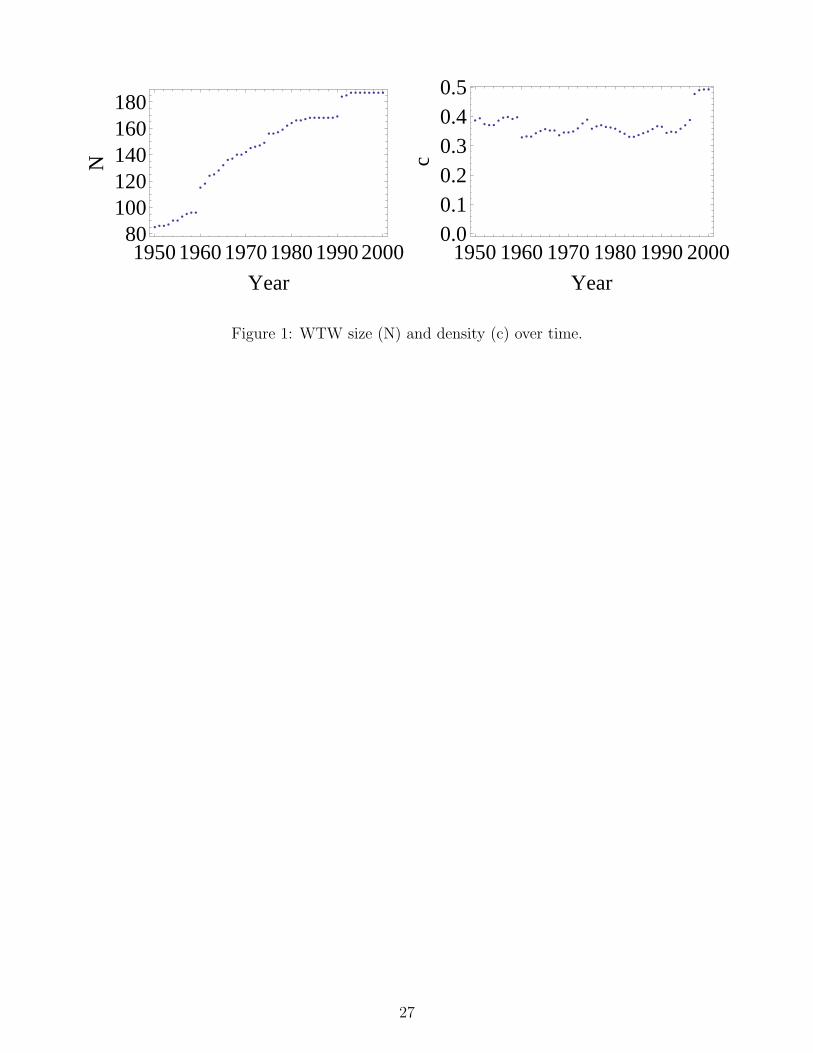
19501960197019801990200080

100120140160180

Year

N• •

• • • • • • • •

• • • • • • • • • • • • • • •• • • • • • • • • • • • • • • •

• • • • • •

• • • •

1950196019701980199020000.00.10.20.30.40.5

Year

c

Figure 1: WTW size (N) and density (c) over time.

27

�

�

����

�

�

����

�

�

��

�

�

�

�

��

�

�

�

�

��

�

�

�

�

��

�

�

�

�

��

�

�

�

�

��

�

�

�

�

��

�

�

�

�

��

�

��

�

��

�

�

�

�

��

�

�

�

�

��

�

�

�

�

�

�

�

�

�

�

�

�

�

�

�

�

�

�

�

�

�

�

�

�

�

�

�

�

�

�

�

�

�

�

�

�

�

�

�

�

�

�

�

�

�

�

�

�

�

�

�

�

�

�

�

�

�

�

�

�

�

�

�

�

�

�

�

�

�

�

�

�

�

�

�

�

�

�

�

�

�

�

�

�

�

�

�

�

�

�

�

�

�

�

�

�

�

�

�

�

�

�

�

�

�

�

�

�

�

�

�

�

�

�

�

�

�

�

�

�

�

�

�

�

�

�

�

�

�

�

�

�

�

�

�

�

�

�

�

�

�

�

�

�

�

�

�

�

�

�

�

�

�

�

�

�

�

�

�

�

�

�

�

�

�

�

�

�

�

�

�

�

�

�

�

�

�

�

�

�

�

�

�

�

�

�

�

�

�

�

�

�

�

�

�

�

�

�

�

�

�

�

�

�

�

�

�

�

�

�

�

�

�

�

�

�

�

�

�

�

�

�

�

�

�

�

�

�

�

�

1950 1960 1970 1980 1990 2000

40

60

80

100

120

140

year

mkin�in,m�kin�in�

a

��

1950 1960 19701.0

0.5

0.0

0.5

1.0

��

������

������

����

�

�

������

�

�

����

�

�

��

�

�

������

������

�

�

��

�

�

����

�

��

�

��

�

�

�

�

��

�

�

�

�

��

�

�

�

�

��

�

�

�

�

�

�

�

�

�

�

�

�

�

�

�

�

�

�

�

�

�

�

�

�

�

�

�

�

�

�

�

�

�

�

�

�

�

�

�

�

�

�

�

�

�

�

��

�

�

�

�

�

�

�

�

�

�

�

�

�

�

�

�

�

�

�

�

�

�

�

�

�

�

�

�

�

�

�

�

�

�

�

�

�

�

�

�

�

�

�

�

�

�

�

�

�

�

�

�

�

�

�

�

�

�

�

�

�

�

�

�

�

�

�

�

�

�

�

�

�

�

�

�

�

�

�

�

�

�

�

�

�

�

�

�

�

�

�

�

�

�

�

�

�

�

�

�

�

�

�

�

�

�

�

�

�

�

�

�

�

�

�

�

�

�

�

�

�

�

�

�

�

�

�

�

�

�

�

�

�

�

�

�

�

�

�

�

�

�

�

�

�

�

�

�

�

�

�

�

�

�

�

�

�

�

�

�

�

�

�

�

�

�

�

�

�

�

�

�

�

�

�

�

1950 1960 1970 1980 1990 2000

40

60

80

100

120

140

year

mkin�out,m�kin�out �

a

��

1950 1960 19701.0

0.5

0.0

0.5

1.0

��

������

������

�

�

��

�

�

����

�

�

�

�

����

����

�

�

����

�

�

����

�

�

����

�

�

����

�

��

�

��

�

�

�

�

��

�

�

�

�

��

�

�

�

�

��

�

�

�

�

�

�

�

�

�

�

�

�

�

�

�

�

�

�

�

�

�

�

�

�

�

�

�

�

�

�

�

�

�

�

�

�

�

�

�

�

�

�

�

�

�

�

�

�

�

�

�

�

�

�

�

�

�

�

�

�

�

�

�

�

�

�

�

�

�

�

�

�

�

�

�

�

�

�

�

�

�

�

�

�

�

�

�

�

�

�

�

�

�

�

�

�

�

�

�

�

�

�

�

�

�

�

�

�

�

�

�

�

�

�

�

�

�

�

�

�

�

�

�

�

�

�

�

�

�

�

�

�

�

�

�

�

�

�

�

�

�

�

�

�

�

�

�

�

�

�

�

�

�

�

�

�

�

�

�

�

�

�

�

�

�

�

�

�

�

�

�

�

�

�

�

�

�

�

�

�

�

�

�

�

�

�

�

�

�

�

�

�

�

�

�

�

�

�

�

�

�

�

�

�

�

�

�

�

�

�

�

�

�

�

�

�

�

�

�

�

�

�

�

�

1950 1960 1970 1980 1990 2000

40

60

80

100

120

140

year

mkout�in,m�kout�in�

a

��

1950 1960 19701.0

0.5

0.0

0.5

1.0

��

������

������

������

������

�

�

����

������

������

������

������

�������

�

��

�

�

�

�

��

�

�

�

�

��

�

�

�

�

��

�

�

�

�

��

�

�

�

�

�

�

�

�

�

�

�

�

�

�

�

�

�

�

�

�

�

�

��

�

�

�

�

��

�

�

�

�

�

�

�

�

�

�

�

�

�

�

�

�

�

�

�

�

�

�

�

�

�

�

�

�

�

�

�

�

�

�

�

�

�

�

�

�

�

�

�

�

�

�

�

�

�

�

�

�

�

�

�

�

�

�

�

�

�

�

�

�

�

�

�

�

�

�

�

�

�

�

�

�

�

�

�

�

�

�

�

�

�

�

�

�

�

�

�

�

�

�

�

�

�

�

�

�

�

�

�

�

�

�

�

�

�

�

�

�

�

�

�

�

�

�

�

�

�

�

�

�

�

�

�

�

�

�

�

�

�

�

�

�

�

�

�

�

�

�

�

�

�

�

�

�

�

�

�

�

�

�

�

�

�

�

�

�

�

�

�

�

�

�

�

�

�

�

�

�

�

�

�

�

�

�

�

�

�

�

�

�

�

�

�

�

1950 1960 1970 1980 1990 2000

40

60

80

100

120

140

year

mkout�out ,m�kout�out �

a

��

1950 1960 19701.0

0.5

0.0

0.5

1.0

year

��

Figure 2: The binary-directed WTW: average nearest neighbor degrees and 95% confidence bands.Red: observed quantities. Blue: null-model fit. Top-left: IN-IN ANND. Top-right: IN-OUTANND. Bottom-left: OUT-IN ANND. Bottom-right: OUT-OUT ANND.

28

�

�

�

�

�

�

�

�

�

�

�

�

�

�

�

�

�

�

�

�

�

�

�

�

�

�

�

�

�

�

�

�

�

�

�

�

�

�

�

�

�

�

�

�

�

�

�

�

�

�

�

�

�

�

�

�

�

�

�

�

�

�

�

�

�

��

��

�

�

�

�

��

�

�

�

�

�

�

�

�

�

�

�

�

�

�

�

�

�

�

�

�

�

�

�

�

�

�

�

�

�

�

�

�

�

�

�

�

�

�

�

�

�

�

�

�

�

�

��

�

�

�

�

�

�

�

�

�

�

�

�

�

�

��

��

�

��

�

��

�

��

�

��

1950 1960 1970 1980 1990 2000�1.0

�0.5

0.0

0.5

1.0

year

rkin�in,�kin�in�

c

�

�

�

�

�

�

�

�

�

�

�

�

�

�

�

�

�

�

�

�

�

�

�

�

�

�

�

�

�

�

�

�

�

�

�

�

�

�

�

�

�

�

�

�

�

�

�

�

�

�

�

�

�

�

�

�

�

�

�

�

�

�

�

�

�

��

��

�

�

�

�

��

�

�

�

�

�

�

�

�

�

�

�

�

�

�

�

�

�

�

�

�

�

�

�

�

�

�

�

�

�

�

�

�

�

�

�

�

�

�

��

�

�

�

��

�

��

�

�

�

�

��

�

��

�

�

�

�

�

��

��

�

��

�

��

�

��

�

��

1950 1960 1970 1980 1990 2000�1.0

�0.5

0.0

0.5

1.0

year

rkin�out ,�kin�out �

c

�

�

�

�

�

�

�

�

�

�

�

�

�

�

�

�

�

�

�

�

�

�

�

�

�

�

�

�

�

�

�

�

�

�

�

�

�

�

�

�

�

�

�

�

�

�

�

�

�

�

�

�

�

�

�

�

�

�

�

�

�

�

�

�

�

�

�

�

�

�

��

�

��

�

�

�

�

��

�

��

�

��

�

�

�

�

�

�

�

�

�

�

�

�

�

�

�

�

�

��

��

�

�

�

�

�

�

�

�

�������

���������

���

���

������

���

������

1950 1960 1970 1980 1990 2000�1.0

�0.5

0.0

0.5

1.0

year

rkout�in,�kout�in�

c

�

�

�

�

�

�

�

�

�

�

�

�

�

�

�

�

�

�

�

�

�

�

�

�

�

�

�

�

�

�

�

�

�

�

�

�

�

�

�

�

�

�

�

�

�

�

�

�

�

�

�

�

�

�

�

�

�

�

�

�

�

�

�

�

�

�

�

�

�

�

�

�

�

�

�

�

�

�

�

�

�

�

�

�

�

�

�

�

�

�

�

�

�

�

�

�

�

�

�

�

�

�

�

�

�

�

�

�

�

�

�

�

�

�

�

�

��

��

���

�

��

�

�����

���

���������

������

���

1950 1960 1970 1980 1990 2000�1.0

�0.5

0.0

0.5

1.0

year

rkout�out ,�kout�out �

c

Figure 3: The binary-directed WTW: Pearson correlation coefficient between observed and null-model node ANND. Top-left: IN-IN ANND. Top-right: IN-OUT ANND. Bottom-left: OUT-INANND. Bottom-right: OUT-OUT ANND.

�

�

�

�

�

�

�

�

�

�

�

�

�

�

�

�

�

�

�

�

�

�

�

�

�

�

�

�

�

�

�

�

�

�

�

�

�

�

�

�

�

�

�

�

�

��

�

�

�

�

�

�

�

�

�

�

�

�

�

��

�

��

�

��

�

���������

������

��

��

�

�

�

�

�

�

�

�

�

�

�

�

�

�

��

�

��

�

�

�

�

��

�

��

�

���

������

���

���

���

���

���

���

���

���

���

������������������������������������������������

������

���

���

���������

���������

���������������������

������

������������������������������������������������

1950 1960 1970 1980 1990 2000�1.0

�0.5

0.0

0.5

1.0

year

rktot�tot ,ktot ,r�ktot�tot �,ktot

c

��

Figure 4: Disassortativity in the binary-directed WTW. Orange: Observed correlation betweentotal ANND and total ND. Green: Correlation between expected total ANND and observed totalND.

29

�

�

�

�

�

�

�

�

�

�

�

�

�

�

�

�

�

�

�

�

�

�

�

�

�

�

�

�

�

�

�

�

�

�

�

�

�

�

�

�

�

�

�

�

�

�

�

�

�

�

�

�

�

�

�

�

�

�

�

�

�

�

�

�

�

�

�

�

�

�

�

�

�

�

�

�

�

�

�

�

�

�

�

�

�

�

�

�

�

�

�

�

�

�

�

�

�

�

�

�

�

�

�

�

�

�

�

�

�

�

�

�

�

�

�

�

�

�

�

�

�

�

�

�

�

�

�

�

�

�

�

�

�

�

�

�

�

�

�

�

�

�

�

�

�

�

�

�

�

�

�

�

�

�

�

�

�

�

�

�

�

�

�

�

�

�

�

�

�

�

�

�

�

�

�

�

�

�

�

�

�

�

�

�

�

�

�

�

�

�

�

�

�

�

�

�

�

�

�

�

�

�

�

�

�

�

�

�

�

�

�

�

�

�

�

�

�

�

�

�

�

�

�

�

�

�

�

�

�

�

�

�

�

�

�

�

�

�

�

�

�

�

�

�

�

�

�

�

�

�

�

�

�

�

�

�

�

�

�

�

�

�

�

�

�

�

�

�

�

�

�

�

�

�

�

�

�

�

�

�

�

��

�

�

�

�

�

�

�

�

�

�

�

�

�

�

�

�

�

�

�

�

�

�

�

1950 1960 1970 1980 1990 20000.0

0.2

0.4

0.6

0.8

1.0

year

mcin,m�cin�

a

��

1950 1960 19701.0

0.5

0.0

0.5

1.0

��

�

�

�

�

�

�

�

�

�

�

�

�

�

�

�

�

�

�

�

�

�

�

�

�

�

�

�

�

�

�

�

�

�

�

�

�

�

�

�

�

�

�

�

�

�

�

�

�

�

�

�

�

�

�

�

�

�

�

�

�

�

�

�

�

�

�

�

�

�

�

�

�

�

�

�

�

�

�

�

�

�

�

�

�

�

�

�

�

�

�

�

�

�

�

�

�

�

�

�

�

�

�

�

�

�

�

�

�

�

�

�

�

�

�

�

�

�

�

�

�

�

�

�

�

�

�

�

�

�

�

�

�

�

�

�

�

�

�

�

�

�

�

�

�

�

�

�

�

�

�

�

�

�

�

�

�

�

�

�

�

�

�

�

�

�

�

�

�

�

�

�

�

�

�

�

�

�

�

�

�

�

�

�

�

�

�

�

�

�

�

�

�

�

�

�

�

�

�

�

�

�

�

�

�

�

�

�

�

�

�

�

�

�

�

�

�

�

�

�

�

�

�

�

�

�

�

�

�

�

�

�

�

�

�

�

�

�

�

�

�

�

�

�

�

�

�

�

�

�

�

�

�

�

�

�

�

�

�

�

�

�

�

�

�

�

�

�

�

�

�

�

�

�

�

�

�

�

�

�

�

�

��

�

�

�

�

�

�

�

�

�

�

�

�

�

�

�

�

�

�

�

�

�

�

�

1950 1960 1970 1980 1990 20000.0

0.2

0.4

0.6

0.8

1.0

year

mcout ,m�cout �

a

��

1950 1960 19701.0

0.5

0.0

0.5

1.0

��

�

�

�

�

�

�

�

�

�

�

�

�

�

�

�

�

�

�

�

�

�

�

�

�

�

�

�

�

�

�

�

�

�

�

�

�

�

�

�

�

�

�

�

�

�

�

�

�

�

�

�

�

�

�

�

�

�

�

�

�

�

�

�

�

�

�

�

�

�

�

�

�

�

�

�

�

�

�

�

�

�

�

�

�

�

�

�

�

�

�

�

�

�

�

�

�

�

�

�

�

�

�

�

�

�

�

�

�

�

�

�

�

�

�

�

�

�

�

�

�

�

�

�

�

�

�

�

�

�

�

�

�

�

�

�

�

�

�

�

�

�

�

�

�

�

�

�

�

�

�

�

�

�

�

�

�

�

�

�

�

�

�

�

�

�

�

�

�

�

�

�

�

�

�

�

�

�

�

�

�

�

�

�

�

�

�

�

�

�

�

�

�

�

�

�

�

�

�

�

�

�

�

�

�

�

�

�

�

�

�

�

�

�

�

�

�

�

�

�

�

�

�

�

�

�

�

�

�

�

�

�

�

�

�

�

�

�

�

�

�

�

�

�

�

�

�

�

�

�

�

�

�

�

�

�

�

�

�

�

�

�

�

�

�

�

�

�

�

�

�

�

�

�

�

�

�

�

�

�

�

�

��

�

�

�

�

�

�

�

�

�

�

�

�

�

�

�

�

�

�

�

�

�

�

�

1950 1960 1970 1980 1990 20000.0

0.2

0.4

0.6

0.8

1.0

year

mccyc,m�ccyc �

a

��

�

1950 1960 19701.0

0.5

0.0

0.5

1.0

year

��

�

�

�

�

�

�

�

�

�

�

�

�

�

�

�

�

�

�

�

�

�

�

�

�

�

�

�

�

�

�

�

�

�

�

�

�

�

�

�

�

�

�

�

�

�

�

�

�

�

�

�

�

�

�

�

�

�

�

�

�

�

�

�

�

�

�

�

�

�

�

�

�

�

�

�

�

�

�

�

�

�

�

�

�

�

�

�

�

�

�

�

�

�

�

�

�

�

�

�

�

�

�

�

�

�

�

�

�

�

�

�

�

�

�

�

�

�

�

�

�

�

�

�

�

�

�

�

�

�

�

�

�

�

�

�

�

�

�

�

�

�

�

�

�

�

�

�

�

�

�

�

�

�

�

�

�

�

�

�

�

�

�

�

�

�

�

�

�

�

�

�

�

�

�

�

�

�

�

�

�

�

�

�

�

�

�

�

�

�

�

�

�

�

�

�

�

�

�

�

�

�

�

�

�

�

�

�

�

�

�

�

�

�

�

�

�

�

�

�

�

�

�

�

�

�

�

�

�

�

�

�

�

�

�

�

�

�

�

�

�

�

�

�

�

�

�

�

�

�

�

�

�

�

�

�

�

�

�

�

�

�

�

�

�

�

�

�

�

�

�

�

�

�

�

�

�

�

�

�

�

�

��

�

�

�

�

�

�

�

�

�

�

�

�

�

�

�

�

�

�

�

�

�

�

�

1950 1960 1970 1980 1990 20000.0

0.2

0.4

0.6

0.8

1.0

year

mcmid,m�cmid�

a

��

1950 1960 19701.0

0.5

0.0

0.5

1.0

��

Figure 5: The binary-directed WTW: average clustering coefficients and 95% confidence bands.Red: observed quantities. Blue: null-model fit. Top-left: BCC In. Top-right: BCC Out. Bottom-left: BCC Cycle. Bottom-right: BCC Middleman.

30

�

�

�

�

�

�

�

�

�

�

�

�

�

�

�

�

�

��

�

�

�

�

�

�

�

�

�

�

�

�

�

�

�

�

�

�

�

�

�

�

�

�

�

�

�

�

�

�

�

�

�

�

�

�

�

�

�

�

�

�

�

�

�

�

��

��

���

���

���

�

��

�

��

�

��

�

�

�

�

��

�

�

�

�

�

�

�

�

�

�

�

�

�

�

�

�

�

�

�

�

����

���

���

�

��

�

��

�

��

�

��

���

������

���

���

���

1950 1960 1970 1980 1990 2000�1.0

�0.5

0.0

0.5

1.0

year

rcin,�cin�

c

�

�

�

�

�

�

�

�

�

�

�

�

�

�

�

�

�

�

�

�

�

�

�

�

�

�

�

�

�

�

�

�

�

�

�

�

�

�

�

�

�

�

�

�

�

�

�

�

�

�

�

�

�

�

�

�

�

�

�

�

�

�

�

�

�

�

�

��������

���

���

���

�

��

�

��

���

���

���

���

���

���

���

������������

���

���������������������������

1950 1960 1970 1980 1990 2000�1.0

�0.5

0.0

0.5

1.0

year

rcout ,�cout �

c

�

�

�

�

�

�

�

�

�

�

�

�

�

�

�

�

�

�

�

�

�

�

�

�

�

�

�

�

�

�

�

�

�

�

�

�

�

�

�

�

�

�

�

�

�

�

�

�

�

�

�

�

�

�

�

�

�

�

�

�

�

�

�

�

�����

������

������

���

���

�

�

�

�

�

�

�

��

�

��

�

�

�

�

��

�

��

�

��

�

�����

���

���

���

���

���

���

�

�

�

���������������

1950 1960 1970 1980 1990 2000�1.0

�0.5

0.0

0.5

1.0

year

rccyc ,�ccyc �

c

�

�

�

�

�

�

�

�

�

�

�

�

�

�

�

�

�

�

�

�

�

�

�

�

�

�

��

�

�

�

�

�

�

�

�

�

�

�

�

�

�

�

�

�

�

�

�

�

�

�

�

��

�

�

�

�

�

�

�

��

�

�����������

������

���

���

���

�

�����

���

���

���

���

���������������

���

���������������������������

1950 1960 1970 1980 1990 2000�1.0

�0.5

0.0

0.5

1.0

year

rcmid,�cmid�

c

Figure 6: The binary-directed WTW: Pearson correlation coefficient between observed and null-model node clustering coefficients and 95% confidence bands. Top-left: BCC In. Top-right: BCCOut. Bottom-left: BCC Cycle. Bottom-right: BCC Middleman.

���������������������������������������������������������������������������������������������������������������������������������������������������������

�

�

�

�

�

�

�

�

�

�

�

�

�

�

�

�

�

�

�

�

�

�

�

�

�

�

�

�

�

�

�

�

�

�

�

�

�

�

�

�

�

�

�

�

�

�

�

�

�

�

�

�

�

�

�

�

�

�

�

�

�

�

�

��

�

���

���

������

������

��

��

�

�

��

�

��

�

��

�

��

�

���

��

�

��

�

���

���

���

������

���

���

������

������

���

���

���

1950 1960 1970 1980 1990 2000�1.0

�0.8

�0.6

�0.4

�0.2

0.0

0.2

0.4

year

rctot ,ktot ,r�ctot �,ktot

c��

Figure 7: Correlation between total binary clustering coefficient and node degree in the binary-directed WTW. Orange: Observed correlation between total BCC and total ND. Green: Correla-tion between expected total BCC and observed total ND.

31

0 20 40 60 80 100 120 1400

20

40

60

80

100

120

ktot

ktot�tot ,�ktot�tot �

a

�tot �

0 50 100 150 200 2500

50

100

150

200

ktot

��

c

��

0 50 100 150 200 250 3000

50

100

150

200

250

300

ktot

��

e

��

0 50 100 150 200 250 3000

50

100

150

200

250

300

ktot

��

e

0 50 100 150 200 250 300 3500

50

100

150

200

250

300

350

ktot

ktot�tot ,�ktot�tot �

f

Figure 8: Disassortativity in the binary WTW. Scatter plots of total ANND vs. observed totalnode degree in 1950 (left) and 2000 (right). Red: observed quantities. Blue: null-model fit.

0 20 40 60 80 100 120 140

0.0

0.2

0.4

0.6

0.8

ktot

ctot ,�ctot �

a

��

0 50 100 150 200 250

0.0

0.2

0.4

0.6

0.8

1.0

ktot

��

c

��

0 50 100 150 200 250 300

0.0

0.2

0.4

0.6

0.8

1.0

ktot

��

e

��

0 50 100 150 200 250 300

0.0

0.2

0.4

0.6

0.8

1.0

ktot

��

e

0 50 100 150 200 250 300 350

0.0

0.2

0.4

0.6

0.8

1.0

ktot

ctot ,�ctot �

f

Figure 9: Clustering coefficient vs. observed total node degree in the binary WTW. Scatter plotsof total BCC vs. ND in 1950 (left) and 2000 (right). Red: observed quantities. Blue: null-modelfit.

32

�

�

�

���

�

�

�

���

�

�

�

���

�

�

�

���

�

�

�

���

�

�

�

���

�

�

�

���

�

�

�

���

�

�

�

���

�

�

�

���

�

�

�

���

�

�

�

���

�

�

�

���

�

�

�

���

�

�

�

���

�

�

�

���

�

�

�

���

�

�

�

���

�

�

�

���

�

�

�

���

�

�

�

���

�

�

�

���

�

�

�

���

�

�

�

���

�

�

�

���

�

�

�

���

�

�

�

���

�

�

�

���

�

�

�

���

�

�

�

���

�

�

�

���

�

�

�

���

�

�

�

���

�

�

�

���

�

�

�

���

�

�

�

���

�

�

�

���

�

�

�

���

�

�

�

���

�

�

�

���

�

�

�

���

�

�

�

���

�

�

�

���

�

�

�

���

�

�

�

���

�

�

�

���

�

�

�

���

�

�

�

���

�

�

�

���

�

�

�

���

�

�

�

���

1950 1960 1970 1980 1990 20000.000

0.005

0.010

0.015

0.020

0.025

0.030

year

ms�in�in,m�s�in�in�

a

��

1950 1960 19701.0

0.5

0.0

0.5

1.0

��

�

�

�

���

�

�

�

���

�

�

�

���

�

�

�

���

�

�

�

���

�

�

�

���

�

�

�

���

�

�

�

���

�

�

�

���

�

�

�

���

�

�

�

���

�

�

�

���

�

�

�

���

�

�

�

���

�

�

�

���

�

�

�

���

�

�

�

���

�

�

�

���

�

�

�

���

�

�

�

���

�

�

�

���

�

�

�

���

�

�

�

���

�

�

�

���

�

�

�

���

�

�

�

���

�

�

�

���

�

�

�

���

�

�

�

���

�

�

�

���

�

�

�

���

�

�

�

���

�

�

�

���

�

�

�

���

�

�

�

���

�

�

�

���

�

�

�

���

�

�

�

���

�

�

�

���

�

�

�

���

�

�

�

���

�

�

�

���

�

�

�

���

�

�

�

���

�

�

�

���

�

�

�

���

�

�

�

���

�

�

�

���

�

�

�

���

�

�

�

���

�

�

�

���

1950 1960 1970 1980 1990 20000.000

0.005

0.010

0.015

0.020

0.025

0.030

year

ms�in�out,m�s�in�out �

a

�

1950 1960 19701.0

0.5

0.0

0.5

1.0

��

�

�

�

���

�

�

�

���

�

�

�

���

�

�

�

���

�

�

�

���

�

�

�

���

�

�

�

���

�

�

�

���

�

�

�

���

�

�

�

���

�

�

�

���

�

�

�

���

�

�

�

���

�

�

�

���

�

�

�

���

�

�

�

���

�

�

�

���

�

�

�

���

�

�

�

���

�

�

�

���

�

�

�

���

�

�

�

���

�

�

�

���

�

�

�

���

�

�

�

���

�

�

�

���

�

�

�

���

�

�

�

���

�

�

�

���

�

�

�

���

�

�

�

���

�

�

�

���

�

�

�

���

�

�

�

���

�

�

�

���

�

�

�

���

�

�

�

���

�

�

�

���

�

�

�

���

�

�

�

���

�

�

�

���

�

�

�

���

�

�

�

���

�

�

�

���

�

�

�

���

�

�

�

���

�

�

�

���

�

�

�

���

�

�

�

���

�

�

�

���

�

�

�

���

1950 1960 1970 1980 1990 20000.000

0.005

0.010

0.015

0.020

0.025

0.030

year

ms�out�in,m�s�out�in�

a

�

1950 1960 19701.0

0.5

0.0

0.5

1.0

��

1950 1960 1970 1980 1990 2000 0

0.005

0.010

0.015

0.020

0.025

0.030

year

ms

out

out ,ms

out

out

Figure 10: The weighted-directed WTW: average nearest neighbor strengths and 95% confidencebands. Red: observed quantities. Blue: null-model fit. Top-left: IN-IN ANNS. Top-right: IN-OUTANNS. Bottom-left: OUT-IN ANNS. Bottom-right: OUT-OUT ANNS.

33

�

�

�

�

�

�

�

�

�

�

�

�

�

�

�

�

�

�

�

�

�

�

�

�

�

�

�

�

�

�

�

�

�

�

�

�

�

�

�

�

�

�

�

�

�

�

�

�

�

�

�

�

�

�

�

�

�

�

�

�

�

�

�

�

�

�

�

�

�

�

�

�

�

�

�

�

�

�

�

�

�

�

�

�

�

�

�

�

�

�

�

�

�

�

�

�

�

�

�

�

�

�

�

�

�

�

�

�

�

�

�

�

�

�

�

�

�

�

�

�

�

�

�

�

�

�

�

�

�

�

�

�

�

�

�

�

�

�

�

�

�

�

�

�

�

�

�

�

�

�

�

�

�

1950 1960 1970 1980 1990 2000�1.0

�0.5

0.0

0.5

1.0

year

rs�in�in,�s�in�in�

c

�

�

�

�

�

�

�

�

�

�

�

�

�

�

�

�

�

�

�

�

�

�

�

�

�

�

�

�

�

�

�

�

�

�

�

�

�

�

�

�

�

�

�

�

�

�

�

�

�

�

�

�

�

�

�

�

�

�

�

�

�

�

�

�

�

�

�

�

�

�

�

�

�

�

�

�

�

�

�

�

�

�

�

�

�

�

�

�

�

�

�

�

�

�

�

�

�

�

�

�

�

�

�

�

�

�

�

�

�

�

�

�

�

�

�

�

�

�

�

�

�

�

�

�

�

�

�

�

�

�

�

�

�

�

�

�

�

�

�

�

�

�

�

�

�

�

�

�

�

�

�

�

�

1950 1960 1970 1980 1990 2000�1.0

�0.5

0.0

0.5

1.0

year

rs�in�out ,�s�in�out �

c

�

�

�

�

�

�

�

�

�

�

�

�

�

�

�

�

�

�

�

�

�

�

�

�

�

�

�

�

�

�

�

�

�

�

�

�

�

�

�

�

�

�

�

�

�

�

�

�

�

�

�

�

�

�

�

�

�

�

�

�

�

�

�

�

�

�

�

�

�

�

�

�

�

�

�

�

�

�

�

�

�

�

�

�

�

�

�

�

�

�

�

�

�

�

�

�

�

�

�

�

�

�

�

�

�

�

�

�

�

�

�

�

�

�

�

�

�

�

�

�

�

�

�

�

�

�

�

�

�

�

�

�

�

�

�

�

�

�

�

�

�

�

�

�

�

�

�

�

�

�

�

�

�

1950 1960 1970 1980 1990 2000�1.0

�0.5

0.0

0.5

1.0

year

rs�out�in,�s�out�in�

c

�

�

�

�

�

�

�

�

�

�

�

�

�

�

�

�

�

�

�

�

�

�

�

�

�

�

�

�

�

�

�

�

�

�

�

�

�

�

�

�

�

�

�

�

�

�

�

�

�

�

�

�

�

�

�

�

�

�

�

�

�

�

�

�

�

�

�

�

�

�

�

�

�

�

�

�

�

�

�

�

�

�

�

�

�

�

�

�

�

�

�

�

�

�

�

�

�

�

�

�

�

�

�

�

�

�

�

�

�

�

�

�

�

�

�

�

�

�

�

�

�

�

�

�

�

�

�

�

�

�

�

�

�

�

�

�

�

�

�

�

�

�

�

�

�

�

�

�

�

�

�

�

�

1950 1960 1970 1980 1990 2000�1.0

�0.5

0.0

0.5

1.0

year

rs�out�out ,�s�out�out �

c

Figure 11: The weighted-directed WTW: Pearson correlation coefficient between observed andnull-model node ANNS. Top-left: IN-IN ANNS. Top-right: IN-OUT ANNS. Bottom-left: OUT-INANNS. Bottom-right: OUT-OUT ANNS.

�

�

�

�

�

�

�

�

�

�

�

�

�

�

�

�

�

�

�

�

�

�

�

�

�

�

�

�

�

�

�

�

�

�

�

�

�

�

�

�

�

�

�

�

�

�

�

�

�

�

�

�

�

�

�

�

�

�

�

�

�

�

�

�

�

�

�

�

�

�

�

�

�

�

�

�

�

�

�

�

�

�

�

�

�

�

�

�

�

�

�

�

�

�

�

�

�

�

�

�

�

�

�

�

�

�

�

�

�

�

�

�

�

�

�

�

�

�

�

�

�

�

�

�

�

�

�

�

�

�

�

�

�

�

�

�

�

�

�

�

�

�

�

�

�

�

�

�

�

�

�

�

�

���������������

��������������������������������������������������

���������������������������

�������������������������

���������������������

���������������

1950 1960 1970 1980 1990 2000

�1.0

�0.5

0.0

0.5

1.0

year

rs�tot�tot ,s�tot ,r�s�tot�tot �,s�tot

c��

Figure 12: Disassortativity in the weighted-directed WTW. Orange: Observed correlation betweentotal ANNS and total NS. Green: Correlation between expected total ANNS and observed totalNS.

34

10�5 10�4 0.001 0.01 0.1

0.02

0.04

0.06

0.08

0.10

s�tot

s�tot ,�s�tot �

�stot �

10�6 10�5 10�4 0.001 0.01 0.1

0.02

0.03

0.04

0.05

0.06

0.07

0.08

s�tot

�s�

c

�stot �

10�6 10�5 10�4 0.001 0.01 0.1

0.02

0.04

0.06

0.08

0.10

s�tot

�s�

e

�stot �

10�6 10�5 10�4 0.001 0.01 0.1

0.02

0.04

0.06

0.08

0.10

s�tot

s�tot ,�s�tot �

�stot �

Figure 13: Disassortativity in the weighted WTW. Scatter plots of total ANNS vs. observed totalnode strength in 1950 (left) and 2000 (right). Red: observed quantities. Blue: null-model fit.

�

�

�

�

�

�

�

�

�

�

�

�

�

�

�

�

�

�

�

�

�

�

�

��

�

�

�

�

��

�

�

�

�

��

�

�

�

�

�

�

�

�

�

�

�

�

�

�

�

�

�

�

�

�

�

�

��

�

�

�

�

�

�

�

�

�

�

�

�

�

�

�

�

�

�

�

�

�

�

�

�

�

�

�

�

�

�

�

�

�

�

�

�

�

�

�

�

�

�

�

�

�

�

�

�

�

�

�

�

�

�

�

�

�

�

�

�

�

�

�

�

�

�

�

�

�

�

�

�

�

�

�

�

�

�

�

�

�

�

�

�

�

�

�

�

�

�

�

�

�

�

�

�

�

�

�

�

�

�

�

�

�

�

�

�

�

�

�

�

�

�

�

�

�

�

�

�

�

�

�

�

�

�

�

�

�

�

�

�

�

�

�

�

�

�

�

�

�

�

�

�

�

�

��

�

�

�

�

���

�

�

�

���

�

�

�

���

�

�

�

���

�

�

�

���

�

�

�

������

���

���

���

���

������

������

������

������

������

������

������

���

1950 1960 1970 1980 1990 20000.00000

0.00002

0.00004

0.00006

0.00008

0.00010

0.00012

0.00014

year

mc�in,m�c�in�

a

��

1950 1960 19701.0

0.5

0.0

0.5

1.0

��

�

�

�

�

�

��

�

�

�

�

�

�

�

�

�

�

�

�

�

�

�

�

�

�

�

�

�

�

�

�

�

�

�

�

�

�

�

�

�

�

�

�

�

�

�

�

�

�

�

�

�

�

�

�

�

�

�

�

�

�

�

�

�

�

�

�

�

�

�

�

�

�

�

�

�

�

�

�

�

�

�

�

�

�

�

�

�

�

�

�

�

�

�

�

�

�

�

�

�

�

�

�

�

�

�

�

�

�

�

�

�

�

�

�

�

�

�

�

�

�

�

�

�

�

�

�

�

�

�

�

�

�

�

�

�

�

�

�

�

�

�

�

�

�

�

�

�

�

�

�

�

�

�

�

�

�

�

�

�

�

�

�

�

�

�

�

�

�

�

�

�

�

�

�

�

�

�

�

�

�

�

�

�

�

�

�

�

�

�

�

�

�

�

�

�

�

�

�

�

�

�

�

�

�

�

�

�

�

�

�

�

�

�

�

�

�

�

�

�

�

�

�

�

�

�

�

�

�

�

�

�

�

�

�

�

�

�

�

�

�

�

�

�

�

����

���

���

���

���

���

���

���

���

������

������

������

������

������

���

1950 1960 1970 1980 1990 20000.00000

0.00002

0.00004

0.00006

0.00008

0.00010

0.00012

0.00014

year

mc�out ,m�c�out �

a

��

1950 1960 19701.0

0.5

0.0

0.5

1.0

��

�

�

�

�

�

��

�

�

�

�

�

�

�

�

�

�

�

�

�

�

�

�

�

�

�

�

�

�

�

�

�

�

�

�

�

�

�

�

�

�

�

�

�

�

�

�

�

�

�

�

�

�

�

�

�

�

�

�

��

�

�

�

�

�

�

�

�

�

�

�

�

�

�

�

�

�

�

�

�

�

�

�

�

�

�

�

�

�

�

�

�

�

�

�

�

�

�

�

�

�

�

�

�

�

�

�

�

�

�

�

�

�

�

�

�

�

�

�

�

�

�

�

�

�

�

�

�

�

�

�

�

�

�

�

�

�

�

�

�

�

�

�

�

�

�

�

�

�

�

�

�

�

�

�

�

�

�

�

�

�

�

�

�

�

�

�

�

�

�

�

�

�

�

�

�

�

�

�

�

�

�

�

�

�

�

�

�

�

�

�

�

�

�

�

�

�

�

�

�

�

�

�

�

�

�

�

�

�

�

�

�

�

�

�

�

�

�

�

�

�

�

�

�

���

�

�

�

���

�

�

�

���

�

�

�

������

���

���

���

���

���

���

������

������

������

������

������

������

���

1950 1960 1970 1980 1990 20000.00000

0.00002

0.00004

0.00006

0.00008

0.00010

0.00012

0.00014

year

mc�cyc,m�c�cyc �

a

��

1950 1960 19700.0

0.2

0.4

0.6

0.8

1.0

��

�

�

�

�

�

��

�

�

�

�

�

�

�

�

�

�

�

�

�

�

�

�

��

�

�

�

�

��

�

�

�

�

�

�

�

�

�

�

�

�

�

�

�

�

�

�

�

�

�

�

�

�

�

�

�

�

��

�

�

�

�

�

�

�

�

�

�

�

�

�

�

�

�

�

�

�

�

�

�

�

�

�

�

�

�

�

�

�

�

�

�

�

�

�

�

�

�

�

�

�

�

�

�

�

�

�

�

�

�

�

�

�

�

�

�

�

�

�

�

�

�

�

�

�

�

�

�

�

�

�

�

�

�

�

�

�

�

�

�

�

�

�

�

�

�

�

�

�

�

�

�

�

�

�

�

�

�

�

�

�

�

�

�

�

�

�

�

�

�

�

�

�

�

�

�

�

�

�

�

�

�

�

�

�

�

�

�

�

�

�

�

�

�

�

�

�

�

�

�

�

�

�

�

�

�

�

�

�

�

�

�

�

�

�

�

�

�

�

�

�

�

�

�

�

�

�

�

���

�

�

�

���

�

�

�

������

���

���

���

���

���

���

������

������

������

������

������

������

���

1950 1960 1970 1980 1990 20000.00000

0.00002

0.00004

0.00006

0.00008

0.00010

0.00012

0.00014

year

mc�mid,m�c�mid�

a

��

1950 1960 19701.0

0.5

0.0

0.5

1.0

year

��

c

Figure 14: The weighted-directed WTW: average weighted clustering coefficients and 95% confi-dence bands. Red: observed quantities. Blue: null-model fit. Top-left: BCC In. Top-right: BCCOut. Bottom-left: BCC Cycle. Bottom-right: BCC Middleman.

35

�

�

�

�

�

�

�

�

�

�

�

�

�

�

�

�

�

�

�

�

�

�

�

�

�

�

�

�

�

�

�

�

�

�

�

�

�

�

�

�

�

�

�

�

�

�

�

�

�

�

�

�

�

�

�

�

�

�

�

�

�

�

�

�

�

�

�

�

�

�

�

�

�

�

�

�

�

�

�

�

�

�

�

�

�

�

�

�

�

�

�

�

�

�

�

�

�

�

�

�

�

�

�

�

�

�

�

��

�

�

�

�

�

�

�

�

�

�

�

�

�

�

�

�

�

�

�

�

�

�

�

�

��

�

��

�

�����

���

���

���

1950 1960 1970 1980 1990 2000�1.0

�0.5

0.0

0.5

1.0

year

rc�in,�c�in�

c

�

�

�

�

�

�

�

�

�

�

�

�

�

�

�

�

�

�

�

�

�

�

�

�

�

�

�

�

�

�

�

�

�

�

�

�

�

�

�

�

�

�

�

�

�

�

�

�

�

�

�

�

�

�

�

�

�

�

�

�

�

�

�

�

�

�

�

�

�

�

��

�

��

�

��

�

��

���

�

��

�

��

�

��

�

�

�

�

�

�

�

��

�

��

�

��

�

��

�

��

���

������

���

���

������

������

���

���

���

���

1950 1960 1970 1980 1990 2000�1.0

�0.5

0.0

0.5

1.0

year

rc�out ,�c�out �

c

�

�

��

�

�

�

�

�

�

�

�

�

�

�

�

�

�

�

�

�

�

�

�

�

�

�

�

�

�

�

�

�

�

�

�

�

�

�

�

�

�

�

�

�

�

�

�

�

�

�

�

�

�

�

�

�

�

�

�

�

�

�

�

�

�

�

�

�

�

�

�

�

�

�

�

�

�

�

�

�

�

�

�

�

�

�

�

�

�

�

�

�

�

�

�

�

�

�

�

�

�

�

�

�

�

�

�

�

�

�

�

�

�

�

�

�

�

�

�

�

�

�

�

�

�

�

�

�

�

�

�

�

�

�

�

�

�

�

�

�

�

�

�

�

�

�

�

�

�

�

�

�

1950 1960 1970 1980 1990 20000.0

0.2

0.4

0.6

0.8

1.0

year

rc�cyc ,�c�cyc �

c

�

�

��

�

�

�

�

�

�

�

�

�

�

�

�

�

�

�

�

�

�

�

�

�

�

�

�

�

�

�

�

�

�

�

�

�

�

�

�

�

�

�

�

�

�

�

�

�

�

�

�

�

�

�

�

�

�

�

�

�

�

�

�

�

�

�

�

�

�

�

�

�

��

�

��

�

��

�

��

�

�

�

�

��

�

�

�

�

�

�

�

�

�

�

�

�

�

�

�

�

�

�

�

��

�

��

�

��

�

��

���

���

���

�

�����

���������

���

���

���

1950 1960 1970 1980 1990 2000�1.0

�0.5

0.0

0.5

1.0

year

rc�mid,�c�mid�

c

Figure 15: The weighted-directed WTW: Pearson correlation coefficient between observed andnull-model node weighted-clustering coefficients and 95% confidence bands. Top-left: BCC In.Top-right: BCC Out. Bottom-left: BCC Cycle. Bottom-right: BCC Middleman.

�

�

� �

�

�

�

�

�

�

�

�

�

�

�

�

�

�

�

�

�

�

�

�

�

�

�

�

�

�

�

�

�

�

�

�

�

�

�

�

�

�

�

�

�

�

�

�

�

�

�

�

�

�

�

�

�

�

�

�

�

�

�

�

�

�

�

�

�

�

�

�

�

�

�

�

�

�

�

�

�

�

�

�

�

�

�

�

�

�

�

�

�

�

�

�

�

�

�

�

�

�

�

�

�

�

�

�

�

�

�

�

�

�

�

�

�

�

�

�

�

�

�

�

�

�

�

�

�

�

�

�

�

�

�

�

�

�

�

�

� ���

���

���

���

�

�

�

�

�

�

�

�

�

�

�

�

�

�

�

�

�

�

�

�

�

�

�

�

�

�

�

�

�

�

�

�

�

�

�

�

�

�

�

�

�

�

�

�

�

�

�

�

�

�

�

�

�

�

�

�

�

�

�

�

�

�

�

�

�

�

�

�

�

�

�

�

�

�

�

�

�

�

�

�

�

�

�

�

�

�

�

�

�

�

�

�

�

�

�

�

�

�

�

�

�

�

�

�

�

�

�

�

�

�

�

�

�

�

�

�

�

�

�

�

�

�

�

�

�

�

�

�

�

�

�

�

�

�

�

�

�

�

�

�

�

�

�

�

�

�

�

�

�

�

�

�

�

1950 1960 1970 1980 1990 2000�1.0

�0.5

0.0

0.5

1.0

year

rc�tot�tot ,c�tot,r�c�tot�tot �,c�tot

c��

Figure 16: Correlation between total weighted clustering coefficient and node strength in theweighted-directed WTW. Orange: Observed correlation between total WCC and total NS. Green:Correlation between expected total WCC and observed total NSD.

36

10�5

10�4 0.001 0.01 0.1

0.0000

0.0001

0.0002

0.0003

0.0004

0.0005

s�tot

c�tot ,�c�tot �

��

106

105

104 0.001 0.01 0.1

0.00000

0.00002

0.00004

0.00006

0.00008

0.00010

0.00012

s�tot

�c�

c

��

106

105

104 0.001 0.01 0.1

0

0.00002

0.00004

0.00006

0.00008

s�tot

��

e

��

10�6

10�5

10�4 0.001 0.01 0.1

0

0.00002

0.00004

0.00006

0.00008

s�tot

c�tot ,�c�tot �

�tot �

Figure 17: Weighted clustering coefficient vs. observed total node strength in the weighted WTW.Scatter plots of total WCC vs. NS in 1950 (left) and 2000 (right). Red: observed quantities. Blue:null-model fit.

37

Topological

Properties

Observed Expected

Binary Link aijaji

pij =xouti xin

j

1+xouti xin

j

pji =xoutj xin

i

1+xoutj xin

i

Degrees kini =

∑

j ajikouti =

∑

j aijktoti = kin

i + kouti

〈kini 〉 = kin

i

〈kouti 〉 = kout

i

〈ktoti 〉 = 〈kin

i 〉+ 〈kouti 〉

ANND knn, inini =

∑j ajik

inj

kini

knn, inouti =

∑j ajik

outj

kini

knn, outini =

∑j aijk

inj

kouti

knn, outouti =

∑j aijk

outj

kouti

knn, toti =

∑j(aij+aji)k

totj

ktoti

〈knn, inini 〉 =

∑j pjik

inj

kini

〈knn, inouti 〉 =

∑j pjik

outj

kini

〈knn, outini 〉 =

∑j pijk

inj

kouti

〈knn, outouti 〉 =

∑j pijk

outj

kouti

〈knn, toti 〉 =

∑j(pij+pji)k

totj

ktoti

Clustering ccyci =∑

j

∑k aijajkaki

kini kouti −k↔i

cmidi =

∑j

∑k aikajiajk

kini kouti −k↔i

cini =∑

j

∑k akiajiajk

kini (kini −1)

couti =∑

j

∑k aikajkaij

kouti (kouti −1)

ctoti =∑

j

∑k(aij+aji)(ajk+akj)(aki+aik)

2[

ktoti (ktoti −1)−2k↔i

]

〈ccyci 〉 =∑

j

∑k pijpjkpki

kini kouti −∑

j pijpji

〈cmidi 〉 =

∑j

∑k pikpjipjk

kini kouti −∑

j pijpji

〈cini 〉 =∑

j

∑k pkipjipjk

2∑

j<k pjipki

〈couti 〉 =∑

j

∑k pikpjkpij

2∑

j<k pijpik

〈ctoti 〉 =∑

j

∑k(pij+pji)(pjk+pkj)(pki+pik)

2[

2∑

j<k(pjipki+pijpik)+2(kini kouti )−2∑

j pijpji

]

Table 1: The Binary WTW: Observed and Expected Topological Properties. Note: ANND stands for Average Nearest-NeighborDegree.

38

Topological

Properties

Observed Expected

Link Weights eijejiwij

〈eij〉 =youti yinj

1−youti yinj

〈eji〉 =youtj yini

1−youtj yini

〈wij〉 =〈eij〉∑i 6=j〈eij〉

Strength sini =∑

j wji

souti =∑

j wij

stoti = sini + souti

〈sini 〉 = sini〈souti 〉 = souti

〈stoti 〉 = stoti

ANNS snn, inini =∑

j ajisinj

kini

snn, inouti =∑

j ajisoutj

kini

snn, outini =∑

j aijsinj

kouti

snn, outouti =∑

j aijsoutj

kouti

snn, toti =∑

j(aij+aji)stotj

ktoti

〈snn, inini 〉 =∑

j pjisinj

〈kini 〉

〈snn, inouti 〉 =∑

j pjisoutj

〈kini 〉

〈snn, outini 〉 =∑

j pijsinj

〈kouti 〉

〈snn, outouti 〉 =∑

j pijsoutj

〈kouti 〉

〈snn, toti 〉 =∑

j(pij+pji)stotj

〈ktoti 〉

Clustering cw, cyci =

∑j

∑k w

1/3ij w

1/3jk w

1/3ki

kini kouti −k↔i

cw, midi =

∑j

∑k w

1/3ik w

1/3jk w

1/3ji

kini kouti −k↔i

cw, ini =

∑j

∑k w

1/3jk w

1/3ji w

1/3ki

kini (kini −1)

cw, outi =

∑j

∑k w

1/3ik w

1/3ij w

1/3jk

kouti (kouti −1)

cw, toti =

∑j

∑k(w

1/3ij +w

1/3ji )(w

1/3jk +w

1/3kj )(w

1/3ki +w

1/3ik )

2[

ktoti (ktoti −1)−2k↔i

]

〈cw, cyci 〉 =

∑j

∑k〈w

1/3ij 〉〈w

1/3jk 〉〈w

1/3ki 〉

〈kini 〉〈kouti 〉−∑

j pijpji

〈cw, midi 〉 =

∑j

∑k〈w

1/3ik 〉〈w

1/3jk 〉〈w

1/3ji 〉

〈kini 〉〈kouti 〉−∑

j pijpji

〈cw, ini 〉 =

∑j

∑k〈w

1/3jk 〉〈w

1/3ji 〉〈w

1/3ki 〉

2∑

j<k pjipki

〈cw, outi 〉 =

∑j

∑k〈w

1/3ik 〉〈w

1/3ij 〉〈w

1/3jk 〉

2∑

j<k pijpik

〈cw, toti 〉 =

∑j

∑k〈w

1/3ij +w

1/3ji 〉〈w

1/3jk +w

1/3kj 〉〈w

1/3ki +w

1/3ik 〉

2[

2∑

j<k(pjipki+pijpik)+2(〈kini 〉〈kouti 〉)−2∑

j pijpji

]

Table 2: The Weighted WTW: Observed and Expected Topological Properties. Note: ANNS stands for Average Nearest-NeighborStrength.

39