nts transportation model user guide - national grid · pdf filejanuary 2015 nts transportation...

NTS Transportation Model User Guide

January 2015

January 2015 NTS Transportation Model User Guide v4.0

2

Document Revision History

Version/Revision Number

Date of Issue Notes

1.0 November 2006

2.0 November 2007 Updated to include the new automatic calculation of both obligated (non-incremental) and incremental entry prices. Format change and minor content addition to make document more user-friendly.

3.0 October 2011 Updated for use with Transportation Model v1.2.2.

4.0 January 2015 Update for using the Transportation Model in Microsoft Excel 2010.


3

Contents

1. Disclaimer .................................................................................................................. 4

2. Introduction ................................................................................................................ 5

2.1. Terminology ........................................................................................................... 6

2.2. Microsoft Excel Solver Add-in ................................................................................ 6

2.3. Spreadsheet Protection ......................................................................................... 6

2.4. Navigating the Transportation Model ..................................................................... 6

2.5. Navigating the Exit Capacity Prices Worksheet .................................................... 7

2.6. Navigating the Baseline Worksheet ....................................................................... 7

2.7. Navigating the Entry Capacity Prices Worksheet .................................................. 8

3. Calculating Exit Capacity Prices ................................................................................ 9

3.1. Running the Transportation Model ........................................................................ 9

3.1.1. Calculating LRMC’s ........................................................................................... 9

3.2. Running the Tariff Models.................................................................................... 10

3.2.1. Calculating Entry and Exit Prices Based on a 50:50 Entry-Exit Split .............. 10

3.2.2. Calculating Administered Exit Prices to meet a Target Exit Revenue ............. 11

4. Calculating Entry Capacity Prices ........................................................................... 12

5. Performing Simple “What-if” Scenario Analysis ...................................................... 13

5.1. Scenario Analysis – “Exit Capacity Prices” Worksheet ....................................... 13

5.1.1. Changing the Reference Node ........................................................................ 13

5.1.2. Changing the Annuitisation Factor .................................................................. 13

5.1.3. Changing the Expansion Constant .................................................................. 13

5.1.4. Changing the Target Exit Revenue ................................................................. 13

5.1.5. Changing Supply and Demand Flows ............................................................. 14

5.2. Scenario Analysis – “Entry Capacity Prices” Worksheet ..................................... 14

5.2.1. Calculating Incremental Entry Capacity ........................................................... 14

6. Performing More Extensive Scenario Analysis ....................................................... 16

6.1. Adding a New Exit Point ...................................................................................... 16

6.2. Adding a New Entry Point .................................................................................... 21

7. Contact Details ........................................................................................................ 28

Appendix 1: “Exit Capacity Prices” Worksheet - Understanding the Transport

and Tariff Model Controls ..................................................................................... 29

Appendix 2: “Exit Capacity Prices” Sheet - Further Details ............................... 31

Appendix 3: “Entry Capacity Prices” Sheet – Further Details ........................... 32

Appendix 4: Using the Transportation Model in Microsoft Excel 2007 ............. 33


4

1. Disclaimer

The Transportation Model has been developed by National Grid to seek to enable transparency of its Gas Charging Methodology in respect of the GB National Transmission System (NTS), and is provided on this understanding. This document is not intended to give a detailed account of the capacity charging methodology; pricing papers and detailed supporting documentation are available on our website at: http://www.nationalgrid.com/uk/Gas/Charges/ The model has been developed using Microsoft Office Excel 2010 (please see Appendix 4 for further information about using the Transportation Model in Microsoft Excel 2007). The Transportation Model has been tested on National Grid’s company operating system (based on Windows 7). The Transportation Model is expected to perform as described below on similar Microsoft Windows based systems such as Windows 2000/Windows NT/Windows XP, however, National Grid cannot guarantee the correct behaviour of the model when operated on other systems. Before using the model, users are asked to satisfy themselves that they are able to comply with the terms of the NTS Charging Model Software Licence Agreement that sets out the terms on which National Grid provide this software.

http://www.nationalgrid.com/uk/Gas/Charges/


5

2. Introduction

National Grid NTS is subject to Transportation Owner (TO) and System Operator (SO) Price Controls set by Ofgem. The allowed revenue, defined by the Price Controls, is collected as follows: NTS TO Allowed Revenue Revenue from other charges (under/over recovery ‘K’ from y-2, DN Pensions deficit revenue and metering revenue) is first deducted. 50% of the remaining NTS TO Allowed Revenue is collected from entry charges from the sale of non-incremental obligated entry capacity. A TO Commodity Charge may be levied to adjust for under or over-recovery (negative charge applied in case of over-recovery). The other 50% of the remaining NTS TO Allowed Revenue is collected from exit capacity charges, which are applied on an administered peak day basis. These charges are based on Long Run Marginal Cost (LRMC) of developing the system to meet increased demand and are determined by exit zone. NTS SO Allowed Revenue The NTS SO Allowed Revenue is collected largely by means of an NTS Entry Commodity and Exit Commodity charge. This is a uniform charge, independent of entry and exit points, and is levied on both NTS entry and NTS exit flows. Revenues are also collected from charges for incremental entry and incremental exit capacity. The Transportation Model is concerned with setting entry capacity auction reserve prices and NTS exit capacity charges. It is also used for setting indicative exit capacity charges when required. For further details of Commodity Charges please see the Quarterly Charge Setting Reports located at http://www.nationalgrid.com/uk/Gas/Charges/Tools.

http://www.nationalgrid.com/uk/Gas/Charges/Tools


6

Notes on the Transportation Model

2.1. Terminology

The title “Transportation Model” represents the complete process of calculating the costs associated with transporting each unit of gas through the National Transmission System (Transport Model) and the conversion of these costs into prices (Tariff Model). Note: The Tariff Model comprises of two halves, Raw (Unadjusted) Prices and Administered Exit Prices.

2.2. Microsoft Excel Solver Add-in

The Microsoft Excel Solver Function needs to be activated for the Transportation Model to work. If it has not already been activated, this can be done as follows:

1. Open the Transportation Model. 2. Add in the Microsoft Excel Solver

a. If using Microsoft Excel 2007, select Excel Options>Add-Ins>Manage Excel

Add-ins>Go. (Please see Appendix 4 for further information on using the Transportation Model in Excel 2007).

b. If using Microsoft Excel 2010, select File>Options>Solver Add-In>OK

3. Tick the Solver Add-in tick box to activate the Solver function.

4. Click OK.

2.3. Spreadsheet Protection

The Transportation Model spreadsheet is not protected as it will not be able to function with protection enabled.

2.4. Navigating the Transportation Model

Upon opening the Transportation Model a dialog box will display as shown in Figure 1. Select Enable Macros to proceed. (Please see Appendix 4 for further information on using the Transportation Model in Microsoft Excel 2007).

Figure 1: Security Warning

The Exit Capacity Prices worksheet should be referred to in relation to exit prices (see Section 3 for more details). Both obligated (non-incremental) and incremental entry prices can be viewed in the Entry Capacity Prices worksheet (see Section 4 for details).


7

2.5. Navigating the Exit Capacity Prices Worksheet

Exit capacity prices are calculated using the Exit Capacity Prices worksheet within the Transportation Model (click on the Exit Capacity Prices worksheet at the bottom of the workbook). The Transport Model controls are located in cells G20:J25. The Tariff Model comprises two halves; Raw (Unadjusted) Prices and Administered Exit Prices. The controls for Unadjusted Prices are located in cells L20:S27 and the controls for Administered Exit Prices are located in cells U20:AC27. Note: The Administered Exit Prices take the negative of the raw LRMCs derived from the Transport Model and adds on the revenue adjustment factor. Essentially, columns L to S show how Entry prices are calculated.

Figure 2: Exit Capacity Prices worksheet

2.6. Navigating the Baseline Worksheet

The Baseline Worksheet contains the baseline data which is within the NTS Licence and information on the Baselines within the Application Window data.

Figure 3: Baseline worksheet


8

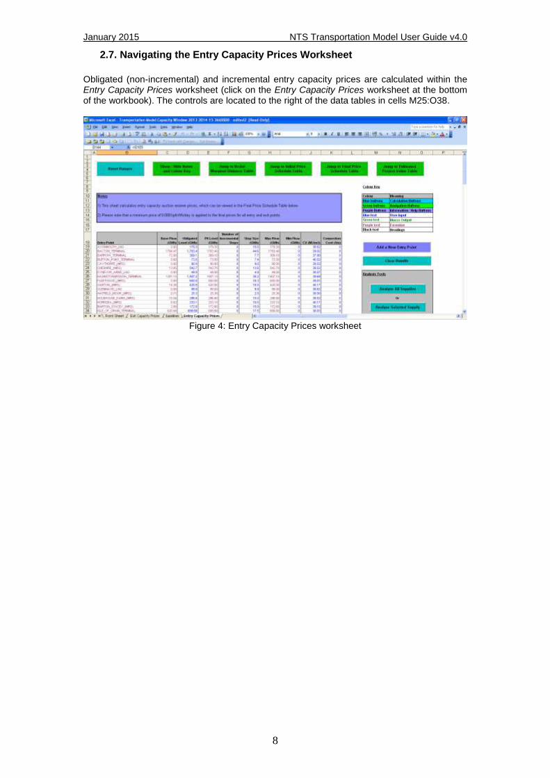
2.7. Navigating the Entry Capacity Prices Worksheet

Obligated (non-incremental) and incremental entry capacity prices are calculated within the Entry Capacity Prices worksheet (click on the Entry Capacity Prices worksheet at the bottom of the workbook). The controls are located to the right of the data tables in cells M25:O38.

Figure 4: Entry Capacity Prices worksheet


9

3. Calculating Exit Capacity Prices

As mentioned in Section 3.5, it is the Exit Capacity Prices worksheet which should only be referred to in relation to exit prices. The function of the worksheet can be summarised as follows:

1. The Transport Model (cells G20:J25) is run to calculate the LRMCs.

2. The LRMCs feed into the first part of the Tariff Model, Tariff Model – Raw (Unadjusted) Prices, which is run to calculate unadjusted entry and exit prices (columns L - S). This Tariff Model simultaneously ensures a 50/50 split between adjusted entry and exit prices, using the Adjustment Factor. This part of the model calculates Entry Capacity prices based on the Supply and Demand Balance, however actual Entry Capacity prices are shown within the Entry Capacity Prices worksheet.

3. The negative of the raw LRMCs derived from the Transport Model (i.e. a positive

Entry LRMC in column J becomes a negative Exit LRMC in columns V to X) then feed into the second part of the Tariff Model, Tariff Model - Administered Prices (columns U – AC), which applies a Revenue Adjustment Factor to the LRMCs so that the Exit Revenue derived from the Exit Capacity charges equals the Target Exit Revenue.

It is the Tariff Model (Administered Prices) that should be referred to for exit prices. More details on the above steps can be found in Sections 3.1 and 3.2 below

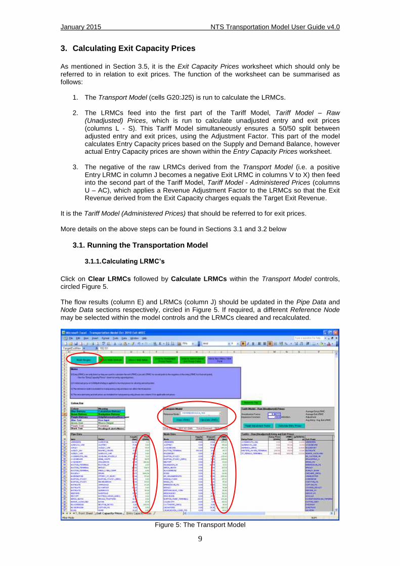
3.1. Running the Transportation Model

3.1.1. Calculating LRMC’s

Click on Clear LRMCs followed by Calculate LRMCs within the Transport Model controls, circled Figure 5. The flow results (column E) and LRMCs (column J) should be updated in the Pipe Data and Node Data sections respectively, circled in Figure 5. If required, a different Reference Node may be selected within the model controls and the LRMCs cleared and recalculated.

Figure 5: The Transport Model


10

Once the LRMCs have been calculated, the Tariff Models may be run. There is no need to rerun the LRMCs if switching between the different Tariff Models. However, the LRMCs will need to be cleared and recalculated if the pipe data or node data is changed. The Reset Ranges button will need to be used before recalculating the LRMCs if additional pipe or node data is entered by the user.

3.2. Running the Tariff Models

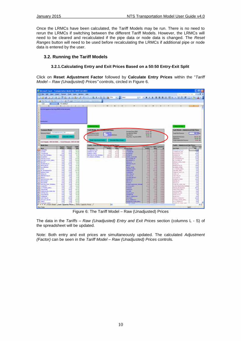
3.2.1. Calculating Entry and Exit Prices Based on a 50:50 Entry-Exit Split

Click on Reset Adjustment Factor followed by Calculate Entry Prices within the “Tariff Model – Raw (Unadjusted) Prices” controls, circled in Figure 6.

Figure 6: The Tariff Model – Raw (Unadjusted) Prices

The data in the Tariffs – Raw (Unadjusted) Entry and Exit Prices section (columns L - S) of the spreadsheet will be updated. Note: Both entry and exit prices are simultaneously updated. The calculated Adjustment (Factor) can be seen in the Tariff Model – Raw (Unadjusted) Prices controls.


11

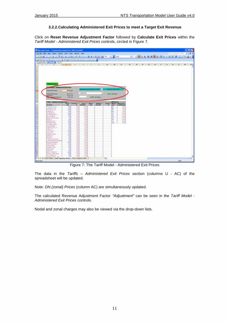
3.2.2. Calculating Administered Exit Prices to meet a Target Exit Revenue

Click on Reset Revenue Adjustment Factor followed by Calculate Exit Prices within the Tariff Model - Administered Exit Prices controls, circled in Figure 7.

Figure 7: The Tariff Model - Administered Exit Prices

The data in the Tariffs – Administered Exit Prices section (columns U - AC) of the spreadsheet will be updated. Note: DN (zonal) Prices (column AC) are simultaneously updated. The calculated Revenue Adjustment Factor “Adjustment” can be seen in the Tariff Model - Administered Exit Prices controls. Nodal and zonal charges may also be viewed via the drop-down lists.


12

4. Calculating Entry Capacity Prices

Obligated (non-incremental) and incremental entry capacity reserve prices (P0 prices) are calculated in the Entry Capacity Prices sheet. This can be done as follows:

1. Click on Reset Ranges before performing any analysis to ensure the model functions correctly.

2. Then either:

a. Select the desired entry point from the drop-down list in the model controls

(columns M – O) and click on Analyse Selected Supply. Or;

b. Click on Analyse All Supplies within the model controls. The Nodal Marginal Distance, Initial Price Schedule and Final Price Schedule tables will all be updated for the selected supply/all supplies. The Final Price Schedule is determined by adjusting the Initial Price Schedule to ensure there is a minimum price step size between successive price steps. Note: The Transportation Model will generate an Excel file for each supply point that is considered - the files will be saved in the same location as the Transportation Model. The generated files do not need to be viewed - they contain more detailed data, which is used to populate the Entry Capacity Prices sheet within the Transportation Model.

Figure 8: The Entry Capacity Prices worksheet


13

5. Performing Simple “What-if” Scenario Analysis

5.1. Scenario Analysis – “Exit Capacity Prices” Worksheet

5.1.1. Changing the Reference Node

The user can change the Reference Node within the Transport Model to observe the effects on the nodal LRMCs. However, it should be noted that this will not affect the final tariffs in either of the two tariff models, as these work by re-referencing the LRMCs to achieve a 50:50 entry-exit split or target exit revenue.

5.1.2. Changing the Annuitisation Factor

The user may change the Annuitisation Factor within the Tariff Model – Raw (Unadjusted) Prices) as determined by National Grid’s NTS Licence to observe the effects on the tariffs in either of the two Tariff Models. This will not affect the LRMCs calculated within the Transport Model.

5.1.3. Changing the Expansion Constant

The user may change the Expansion Constant within the Tariff Model – Raw (Unadjusted) Prices) to observe the effects on the tariffs in either of the two Tariff Models. This will not affect the LRMCs (marginal distances) calculated within the Transport Model.

Figure 9: Changing the Reference Node, Annuitisation Factor and Expansion Constant

5.1.4. Changing the Target Exit Revenue

The user may change the Target Exit Revenue within the Tariff Model - Administered Exit Prices controls to observe the effects on the Administered Exit Prices. This will not affect the LRMCs calculated within the Transport Model or the tariffs calculated from assuming a 50:50 entry-exit split.


14

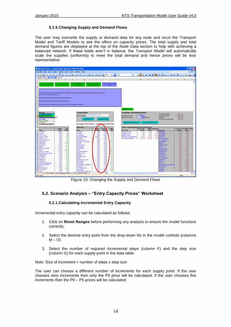
5.1.5. Changing Supply and Demand Flows

The user may overwrite the supply or demand data for any node and rerun the Transport Model and Tariff Models to see the effect on capacity prices. The total supply and total demand figures are displayed at the top of the Node Data section to help with achieving a balanced network. If these totals aren’t in balance, the Transport Model will automatically scale the supplies (uniformly) to meet the total demand and hence prices will be less representative.

Figure 10: Changing the Supply and Demand Flows

5.2. Scenario Analysis – “Entry Capacity Prices” Worksheet

5.2.1. Calculating Incremental Entry Capacity

Incremental entry capacity can be calculated as follows:

1. Click on Reset Ranges before performing any analysis to ensure the model functions correctly.

2. Select the desired entry point from the drop-down list in the model controls (columns

M – O)

3. Select the number of required incremental steps (column F) and the step size (column G) for each supply point in the data table.

Note: Size of increment = number of steps x step size The user can choose a different number of increments for each supply point. If the user chooses zero increments then only the P0 price will be calculated. If the user chooses five increments then the P0 – P5 prices will be calculated.


15

Please refer to the Entry Capacity Release Methodology Statement (ECR), which can be accessed at the following link, for details on selecting the number of required increments and size of step. http://www2.nationalgrid.com/UK/Industry-information/Gas-capacity-methodologies/Entry-Capacity-Release-Methodology-Statement/

4. Click on Analyse Selected Supply or Analyse All Supplies within the model controls.

The Nodal Marginal Distance, Initial Price Schedule, Final Price Schedule, and Estimated Project Value tables will all be updated for the selected supply/all supplies.

Figure 11: Changing the number of Increments and size of step

Note: The Transportation Model will generate an Excel file for each supply point that is considered - the files will be saved in the same location as the Transportation Model. The generated files do not need to be viewed - they contain more detailed data, which is used to populate the Entry Capacity Prices sheet within the Transportation Model.

http://www2.nationalgrid.com/UK/Industry-information/Gas-capacity-methodologies/Entry-Capacity-Release-Methodology-Statement/



16

6. Performing More Extensive Scenario Analysis

6.1. Adding a New Exit Point

It is advisable to save a separate copy of the Transportation Model for scenario analysis. It is possible to add a new exit point into the model in the Exit Capacity Prices worksheet. All new exit points must be connected to a pipe in the network and all pipes must be connected such that there are no isolated sections of the network. In this example we are going to add a new exit point halfway between Horndon and Stanford le Hope (current pipe length 4.06km).

1. Select the Exit Capacity Prices worksheet.

2. Select the Add a New Entry / Exit Point button (cells I2:K4) to bring up the window as in Figure 12.

Figure 12 – the Add a New Entry / Exit Point window

3. In this example please note the following;

The New Exit Point check box has been selected.

In the New Node text box “NEW_EXIT” has been entered as the new exit point name, and “HORNDON” has been selected as the Existing Node.

The Demand quantity (GWh/d) has been entered as “10”.

The Length of pipe (km) has been entered as “2”.

4. Select Populate and Close.

5. The result is that an existing Inlet “HORNDON” has been added to the bottom of the Pipe Data section in column B as has the new exit point, “NEW_EXIT”, which will be connected to the network. The pipe length between the two nodes has also been entered as “2.00” (km).


17

6. We have effectively split the pipe that existed between HORNDON and STANFORD_LE_HOPE into two sections…almost! For completeness, we will now manually enter the remaining information to complete the pipe section between NEW_EXIT and STANDFORD_LE_HOPE as in Figure 13. The remaining pipe length is derived from 4.06km – 2km = 2.06km.

Note: You do not need to enter flow data in column E as this will be populated when the Transport Model is run. Also note that the model is case sensitive i.e. “NEW_EXIT” is different to “New_Exit”, and separate words also need to be joined by using an underscore.

Figure 13: Completing the Pipe Data section


18

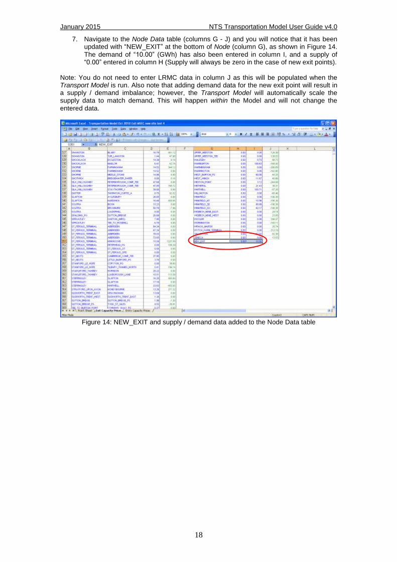
7. Navigate to the Node Data table (columns G - J) and you will notice that it has been updated with “NEW_EXIT” at the bottom of Node (column G), as shown in Figure 14. The demand of “10.00” (GWh) has also been entered in column I, and a supply of “0.00” entered in column H (Supply will always be zero in the case of new exit points).

Note: You do not need to enter LRMC data in column J as this will be populated when the Transport Model is run. Also note that adding demand data for the new exit point will result in a supply / demand imbalance; however, the Transport Model will automatically scale the supply data to match demand. This will happen within the Model and will not change the entered data.

Figure 14: NEW_EXIT and supply / demand data added to the Node Data table


19

8. Navigate to the Tariffs – Raw (Unadjusted) Entry and Exit Prices table (columns L – S). You will notice that “NEW_EXIT” has been added to the bottom of Exit Point

column (column P), as shown in Figure 15, and that the following formulae from the row above have been copied down to the new row entry;

Exit Flow (column Q)

Exit LRMC (column R)

Exit Price (column S) The cells may display “#N/A” but this is expected at this stage.

Figure 15: Updated Tariffs – Raw (Unadjusted) Entry and Exit Prices table

9. Navigate to the Tariffs – Administered Exit Prices table (columns U – AC). You will

notice that “NEW_EXIT” has been added to the bottom of Exit Point column (column U) and that the flow data and formulae from the row above have also been copied down to the new row.

Note: The value for flow (demand) data should be the same as entered earlier in this process i.e. “10”; however, because the data from the row above has been copied down, in this example, “60” has been copied to “NEW_EXIT”. This needs to be amended manually. If “NEW_EXIT” is a Distribution Network Zone enter the relevant code in DN Exit Zone (column Y), otherwise leave this cell blank. Copy the formulae from the following columns into the new row;

DN Offtake Flow (column Z)

Flow*Exit Charge (column AA) Again, the cells may display “#N/A” – this is expected at this stage.


20

10. Within the Baseline worksheet, add in the relevant information relating to the new Entry point. This will be available in the NTS Licence and in the baseline in the Application Window data.

a. If you are not aware of the baseline for the “NEW_EXIT” point then add zeros into the fields within the worksheet as these fields need to be populated.

Figure 16: Baseline Worksheet – Adding Relevant Entry data

11. Click on Reset Ranges in the top left-hand corner of the worksheet. The Transport

Model and Tariff Models can then be run as normal. The results can be viewed in the Tariffs – Administered Exit Charges table (columns U – AC).

Note: “NEW_EXIT” will not appear in the drop-down lists in the Transport Model and Tariff Model. The user has the choice to either:

a. Manually type “NEW EXIT” in the drop down box, overwriting the displayed exit point.

Or;

b. Save, close and re-open the spreadsheet, which will allow the drop-down list to refresh. “NEW_EXIT” will then appear at the bottom of the drop-down lists in the Transport Model and Tariff Model - Administered Exit Prices controls.


21

6.2. Adding a New Entry Point

It is advisable to save a separate copy of the Transportation Model for scenario analysis. It is possible to add a new entry point into the model in the Exit Capacity Prices worksheet. Incremental entry capacity requested in Gas Year 0 will be released in Gas Year 4. The Transportation Model relevant to Gas Year 3 will be used to calculate the entry capacity auction reserve prices for Gas Year 4. For example, if incremental entry capacity is requested through the 2015 QSEC auction, the 2017/18 Transportation Model will be used to calculate the price schedule. Please refer to the Entry Capacity Release Methodology Statement (ECR), which can be accessed at the following link, for details on selecting the number of required increments and size of the step. http://www2.nationalgrid.com/UK/Industry-information/Gas-capacity-methodologies/Entry-Capacity-Release-Methodology-Statement/ A Note on New Entry Points The Transportation Model will not produce the correct incremental prices under two circumstances:

1. 1. If a new entry point is directly connected to an existing entry point via a minimum connection (i.e. a pipe length of 0km between the Inlet and Outlet in the Pipe Data table in the Entry-Exit worksheet)

2. If a new entry point is connected to an existing node that is connected to an existing entry point via a minimum connection.

This can be overcome by entering a small connection (e.g. 0.01km) between the Inlet and Outlet in the Pipe Data table. Example: Direct Minimum Connections to Existing Entry Points The user connects a new entry point, in this example “New Entry”, to existing entry point “Entry Point A” with a minimum connection. The Transportation Model will calculate that they are in the same location and perform all analysis based on only one of the entry points. If the user enters a length of 0km between the two entry points in the Pipe Data table, the Transportation Model will treat the two sites as one entry point and will not function correctly. Example: Indirect Minimum Connections to Existing Entry Points The user connects a new entry point in this example “New Entry” to existing node “Node A” with a minimum connection. However, Node A is connected to existing entry point “Entry Point A” with a minimum connection. Therefore, New Entry is indirectly connected to Entry Point A with a minimum connection. The Transportation Model will calculate that New Entry and Entry Point A are in the same location and perform all analysis based on only one of the entry points.

0km

NEW ENTRY ENTRY POINT A

NEW ENTRY ENTRY POINT A 0km

0km 0km

NODE A




22

A new entry point can be added as follows:

1. Select the Exit Capacity Prices worksheet

2. Select the Add a New Entry / Exit Point button (cells I2:K4) to bring up the window as in Figure 17.

Figure 17 – the Add a New Entry / Exit Point window

3. In this example please note the following;

The New Entry Point check box has been selected. In the New Node text box “NEW_ENTRY” has been entered as the new entry point name, and “HORNDON” has been selected as the Existing Node.

The Supply quantity (GWh/d) has been entered as zero (always zero for new entry points).

The Length of pipe (km) has been entered as zero (always zero for minimum connections).

The Obligate Entry Capacity has been entered as zero (always zero for new entry points).

The Number of Incremental Steps and Step Size have been entered as zero. (The number of incremental steps multiplied by the step size should equal the size of the new entry point.)

Please refer to the Entry Capacity Release Methodology Statement (ECR), which can be accessed at the following link, for details on selecting the number of required increments and size of step. http://www2.nationalgrid.com/UK/Industry-information/Gas-capacity-methodologies/Entry-Capacity-Release-Methodology-Statement/

The CV has been left at its default value of 39.6MJ/m3, however users can amend this if the actual figure is known.

Minimum Flow has been left at zero (always zero for new entry points).

The Connection Cost has been left at zero (always zero for a minimum connection).




23

4. Select Populate and Close The result is that “HORNDON” has been added to the bottom of the Pipe Data section in column B as has the new entry point, “NEW_ENTRY”, which will be connected to the network as shown in Figure 18.

Figure 18: the updated Pipe Data table

Note: You do not need to enter flow data in column E as this will be populated when the Transport Model is run. Also note that the model is case sensitive i.e. “NEW_ENTRY” is different to “New_Entry”, and separate words also need to be joined by using an underscore.


24

5. Navigate to the Node Data table and you will notice that it has been updated with “NEW_ENTRY” to the bottom of Node (column G), as shown in Figure 19. The supply and demand values of “0.00” (GWh) have also been entered in columns H & I respectively (these are always zero in the case of new entry points).

Note: You do not need to enter LRMC data in column J as this will be populated when the Transport Model is run. This will happen within the Model and will not change the entered data.

Figure 19: the updated Node Data table


25

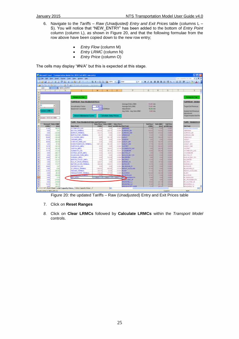
6. Navigate to the Tariffs – Raw (Unadjusted) Entry and Exit Prices table (columns L – S). You will notice that “NEW_ENTRY” has been added to the bottom of Entry Point

column (column L), as shown in Figure 20, and that the following formulae from the row above have been copied down to the new row entry;

Entry Flow (column M)

Entry LRMC (column N)

Entry Price (column O) The cells may display “#N/A” but this is expected at this stage.

Figure 20: the updated Tariffs – Raw (Unadjusted) Entry and Exit Prices table

7. Click on Reset Ranges

8. Click on Clear LRMCs followed by Calculate LRMCs within the Transport Model

controls.


26

9. Click on Reset Adjustment Factor followed by Calculate Entry Prices within the Tariff Model controls (this calculates the adjusted LRMC and Unscaled Entry Capacity prices).

Figure 21: Calculating LRMCs and Unscaled Entry Prices

10. Navigate to the Entry Capacity Prices worksheet. You will notice that “NEW_ENTRY”

has been added to the first table and the previously entered data has also been populated into the appropriate column.

Note: If this is not populated with the “NEW_ENTRY” point then select the last row in the table and copy the values down, this will populate the row below with the appropriate data.


27

11. Click on Reset Ranges in the Entry Capacity Prices worksheet. Note: The “NEW_ENTRY” will not appear in the drop-down lists in the Analysis Tools section, therefore you will need to save, close and re-open the spreadsheet, which will allow the drop-down list to refresh.

Figure 22: The Reset Ranges button and Analysis Tools controls

12. Then either:

a. Select the desired entry point from the drop-down list in the model controls (columns M – O) and click on Analyse Selected Supply.

Or;

b. Click on Analyse All Supplies within the model controls. The Nodal Marginal Distance, Initial Price Schedule and Final Price Schedule tables will all be updated for the selected supply/all supplies. The Final Price Schedule is determined by adjusting the Initial Price Schedule to ensure there is a minimum price step size between successive price steps. Note: The Transportation Model will generate an Excel file for each supply point that is considered - the files will be saved in the same location as the Transportation Model. The generated files do not need to be viewed - they contain more detailed data, which is used to populate the Entry Capacity Prices sheet within the Transportation Model.


28

7. Contact Details

If you experience any difficulties using the model, please contact Colin Williams (01926 655916), Karin Elmhirst (01926 655540) or Laura Butterfield (01926 656160) or alternatively e-mail our Gas Capacity and Charging Development Team on [email protected]


29

Appendix 1: “Exit Capacity Prices” Worksheet - Understanding the Transport and Tariff Model Controls

The controls for the Transport and Tariff Models are described below, in the order that they appear as you navigate across the spreadsheet from left to right. Reset Ranges This function resets the range names within the spreadsheet. Therefore it is only necessary to use this function if Nodes, Entry Points, Exit Points or DN Zones are added by the user.

Transport Model Reference Node It is possible to select a different reference node via the drop-down list of nodes in the network. This will only affect the initial marginal cost values but not the final tariff values. Adjustment of the marginal costs to achieve a 50:50 entry-exit split, or to meet a Target Exit Revenue, will re-reference the marginal costs, so the final tariffs are unaffected. Clear LRMCs It is good practice to clear the LRMCs from a previous calculation before recalculating, especially if more advanced scenario analysis is being undertaken (see below). This clears the LRMC values from the nodal data section and also clears the flow results from the pipe data section. Calculate LRMCs This calculates a set of LRMCs and writes the results in the Node Data section.

Tariff Model – Raw (Unadjusted) Prices Annuitisation Factor The Annuitisation Factor may be changed. The default value of 0.10272 is the annuitisation factor as referred to in Section Y of the UNC.. Expansion Constant The Expansion Constant may be changed. The default value of £2559/GWh km is that used in the published indicative charges for the charging consultation GCM01 and discussion GCD01, available at http://www.nationalgrid.com/uk/Gas/Charges. Reset Adjustment Factor The adjustment factor should always be reset to zero before calculating new entry and exit prices, to ensure consistent calculations are performed. Calculate Entry Prices This calculates a set of entry and exit prices based on a 50:50 entry-exit split. The results are displayed in the Tariffs – Raw (Unadjusted) Entry and Exit Prices section of the spreadsheet. This calculation has been used to determine all baseline and incremental entry prices for GCM01 and all exit prices for GCD01 (enduring exit prices). Average Entry LRMC This is the average of the adjusted entry LRMCs such that all negative adjusted LRMCs are collared at zero or 0.0001. Average Exit LRMC This is the average of the adjusted exit LRMCs such that all negative adjusted LRMCs are collared at zero or 0.0001 Adjustment Factor A constant Adjustment Factor is added to each entry point LRMC and subtracted from each exit LRMC such that the average of the entry costs equals the average of the exit costs, and


30

on average a 50:50 split of charges between entry and exit is achieved. The built in Excel Solver is used to perform this calculation. Avg. Entry – Average LRMC This is the difference between the Average Entry LRMC and Average Exit LRMC, and is used in the Excel Solver to find the Adjustment Factor. This value should be zero (or very close to zero) when the final entry and exit prices are calculated.

Tariff Model – Administered Exit Prices Target Exit Revenue In order to calculate administered exit charges, a Target Exit Revenue figure must be set (in £m), to reflect the proportion of TO allowable revenue to be collected from exit capacity charges. Implied Exit Revenue Prior to the adding of the Revenue Adjustment Factor, the Implied Exit Revenue is the total exit revenue generated if the exit charges were calculated using the LRMCs in column J. (Note: The LRMCs in column J are Entry LRMCs and therefore to calculate Exit Capacity charges the opposite value is used i.e. positive Entry LRMCs become negative Exit LRMCs and vice versa). The Excel Solver is used to find the Revenue Adjustment Factor such that the Implied Exit Revenue equals the Target Exit Revenue. Adjustment The Revenue Adjustment Factor is a constant added to each LRMC value to generate a set of exit charges that will collect the Target Exit Revenue. The Excel Solver is used to find the value of the Revenue Adjustment Factor. Target – Implied Exit Revenue This is the difference between the Target Exit Revenue and Implied Exit Revenue used in the Excel Solver to find the Revenue Adjustment Factor. This value should be zero (or very close to zero) when the final administered charges are calculated. Reset Revenue Adjustment Factor The revenue adjustment factor should always be reset to zero before calculating new exit charges, to ensure consistent calculations are performed. Calculate Exit Prices The Excel Solver is used to adjust the revenues arising from exit charges to match the Target Exit Revenue. The final charges are then displayed in the Tariffs – Administered Exit Charges section of the spreadsheet. Selection of Exit Charges Individual exit points may be selected via the drop down list. Alternatively, the exit charge results may be viewed in the Tariffs – Administered Exit Charges section of the spreadsheet. Selection of Zonal Charges DN charging zones may be selected via the drop down list. Alternatively, the zonal exit charge results may be viewed in the Tariffs – Administered Exit Charges section of the spreadsheet.


31

Appendix 2: “Exit Capacity Prices” Sheet - Further Details

Transport and Tariff Model Controls The controls for the Transport and Tariff Models are linked to the macros used to automate the spreadsheet calculations. Pipe Data (Columns B – E) The first set of data describe the pipes in the underlying network model i.e. pipe inlets, pipe outlets, and pipe lengths. Flows through pipes calculated by the Transport Model are also written to this section of the spreadsheet. (Note: Where more than one route between two nodes of the network exists, the Transport Model chooses the one that has the least cost (in terms of flow distances) so some pipe sections will have no flow through them. If a negative flow value is calculated, it means that the flow is reversed in the pipe i.e. from “outlet” to “inlet”.) Node Data (Columns G – J) Node Data is shown to the right of the Pipe Data and comprises node names, supply flows into the node, demand flows out of the node and LRMCs calculated from the Transport Model. The reference node is shown above the node data, as well as totals for the nodal supply and demand data. Tariffs – Raw (Unadjusted) Entry and Exit Prices (Columns L – S) The data and results to the right of the Node Data are used for the calculation of unadjusted entry and exit prices. There are two blocks of data: one for entry and one for exit. The information is ordered as follows: the entry/exit point names, supply/demand flows referenced from the Node Data section, adjusted values of the LRMCs and prices in p/kWh/day. The adjustment to LRMC values is made so that, on average, 50% of charges are levied on entry and 50% on exit. Tariffs - Administered Exit Prices (Columns U – AC) The second tariff model uses the data to the right of the Tariffs – Raw (Unadjusted) Entry and Exit Prices section. The data is ordered as follows: exit point name, baseline, revenue generated at exit point (assuming the demand flow at the point), and exit charge. A flow is attributed to the Bacton - Zeebrugge Interconnector to account for firm exit capacity at this point.


32

Appendix 3: “Entry Capacity Prices” Sheet – Further Details

Initial Data Table (Range B19 – K41) The first set of data contains the information relevant to calculating incremental entry capacity charges. “Number of Incremental Steps” (column F) needs to be populated by the user. Incremental Entry Controls (Range M25:O38) The Analyse Selected Supply and Analyse All Supplies buttons are linked to macros used to automate the spreadsheet calculations. The required entry point can be selected from the drop-down list. Each time a new entry point is selected the “Reset Ranges” button should be used. Selection of Entry Prices Individual entry points may be selected via the drop down list. Nodal Incremental Distances (Range B24:X76) The first set of data below the Initial Data table contains the Nodal Incremental Distances. Nodal Marginal Distances for the selected supply point/all supplies are converted to Nodal Incremental Distances by calculating the difference between the Nodal Marginal Distance at the incremental level and the Nodal Marginal Distance at the obligated capacity level. Initial Price Schedule (Range B89:X111) The Nodal Incremental Distances are converted to capital costs by multiplying by the Expansion Constant, and annuitised according to the annuitisation factor specified in the Licence. Annuitised costs are converted to p/kWh/day and adjusted to recognise the different calorific values of gas entering the system. The initial incremental step price is calculated by adding the annuitised cost for the incremental capacity step to the obligated entry capacity reserve P0 price. Final Price Schedule (Range B124:X146) The process for determining the Initial Price Schedule will usually result in an increasing price progression with increasing capacity level. However, a price progression that decreases with the incremental capacity level may be observed. In order to test for the presence of an ascending or descending curve, the price at the highest capacity level will be compared to the P1 price. The final incremental step price is determined by ensuring that there is a difference of at least 0.0001p/kWh/day between each incremental step price. Estimated Project Value (Range B159:X181) For the purposes of determining the required commitment from bidders that trigger the release of incremental capacity an estimated project value is calculated for each incremental capacity level from the final incremental step prices.


33

Appendix 4: Using the Transportation Model in Microsoft Excel 2007

Security Warning In Microsoft Excel 2007 there is no Security Warning dialogue box but the warning will be displayed underneath the ribbon bar.

In order to be able to run the Transportation Model select Options to display the following dialogue box, and check the Enable this Content control and click OK.

Solver Error 2007 Some users may experience the following error when running the Transportation Model in Microsoft Excel 2007.


34

To run the Transportation Model in Microsoft Excel 2007 you may need to perform the following steps. 1. Enable the Developer tab by going into Excel Options>Popular, and selecting the Show

Developer tab in the ribbon check box.

2. From the Developer tab select Visual Basic and from the Visual Basic window select

Tools>References

3. You will be presented with the window below. Deselect Missing.Solver.xla

4. Select Solver just beneath it.

5. Click OK, and close the Transportation Model saving changes.

nts transportation model user guide - national grid · pdf filejanuary 2015 nts transportation...

Documents