Report Issued: October 25, 2016

Disclaimer: This report is released to inform interested parties of research and to encourage discussion.

The views expressed are those of the authors and not necessarily those of the U.S. Census Bureau .

STUDY SERIES (Statistics #2016-01)

NSF GRIP Report:

American Community Survey

Simulation Study

Claire McKay Bowen 1

1 Statistics Ph.D. Candidate, University of Notre Dame

Center for Statistical Research & Methodology Research and Methodology Directorate

U.S. Census Bureau Washington, D.C. 20233

Contents

1 American Community Survey Data Summary 41.1 Summary of Raw Data . . . . . . . . . . . . . . . . . . . . . . . . . . . . . . . . . . . 4

1.1.1 Reduction of Data . . . . . . . . . . . . . . . . . . . . . . . . . . . . . . . . . 41.2 Pre-processing the Data Details . . . . . . . . . . . . . . . . . . . . . . . . . . . . . . 5

1.2.1 Changing Continuous Variables to Categorical Variables . . . . . . . . . . . . 51.2.2 Reducing the Classes for Categorical Variables . . . . . . . . . . . . . . . . . 51.2.3 Further Pre-Processing of the Data . . . . . . . . . . . . . . . . . . . . . . . . 6

2 Simulation Study 82.1 Differential Privacy . . . . . . . . . . . . . . . . . . . . . . . . . . . . . . . . . . . . . 82.2 Generation of Synthetic Data . . . . . . . . . . . . . . . . . . . . . . . . . . . . . . . 9

2.2.1 Notation . . . . . . . . . . . . . . . . . . . . . . . . . . . . . . . . . . . . . . . 92.2.2 Assumptions . . . . . . . . . . . . . . . . . . . . . . . . . . . . . . . . . . . . 92.2.3 Model-Based Differentially Private Data Synthesis . . . . . . . . . . . . . . . 102.2.4 Proposed Model . . . . . . . . . . . . . . . . . . . . . . . . . . . . . . . . . . 102.2.5 Range of ε . . . . . . . . . . . . . . . . . . . . . . . . . . . . . . . . . . . . . . 112.2.6 Overall Simulation Steps . . . . . . . . . . . . . . . . . . . . . . . . . . . . . . 11

3 Simulation Results 123.1 Combination Rules for Multiple Synthesis . . . . . . . . . . . . . . . . . . . . . . . . 123.2 Plots . . . . . . . . . . . . . . . . . . . . . . . . . . . . . . . . . . . . . . . . . . . . . 133.3 Bias . . . . . . . . . . . . . . . . . . . . . . . . . . . . . . . . . . . . . . . . . . . . . 133.4 Root Mean Squared Error . . . . . . . . . . . . . . . . . . . . . . . . . . . . . . . . . 133.5 Coverage Probability . . . . . . . . . . . . . . . . . . . . . . . . . . . . . . . . . . . . 143.6 Empty Cells . . . . . . . . . . . . . . . . . . . . . . . . . . . . . . . . . . . . . . . . . 143.7 Conclusion . . . . . . . . . . . . . . . . . . . . . . . . . . . . . . . . . . . . . . . . . 14

A NSF GRIP Overview 19A.1 NSF GRIP Proposal . . . . . . . . . . . . . . . . . . . . . . . . . . . . . . . . . . . . 19

A.1.1 Overview . . . . . . . . . . . . . . . . . . . . . . . . . . . . . . . . . . . . . . 19A.1.2 Research Proposal . . . . . . . . . . . . . . . . . . . . . . . . . . . . . . . . . 21

B NSF GRIP Professional Development and Research 22B.1 Research Products . . . . . . . . . . . . . . . . . . . . . . . . . . . . . . . . . . . . . 23

B.1.1 Dissertation . . . . . . . . . . . . . . . . . . . . . . . . . . . . . . . . . . . . . 23

1

B.1.2 Research Presentations . . . . . . . . . . . . . . . . . . . . . . . . . . . . . . . 23B.1.3 Collaborative Research . . . . . . . . . . . . . . . . . . . . . . . . . . . . . . . 23

B.2 Professional Development . . . . . . . . . . . . . . . . . . . . . . . . . . . . . . . . . 23B.2.1 Expanded Professional Networks . . . . . . . . . . . . . . . . . . . . . . . . . 23B.2.2 Presentation . . . . . . . . . . . . . . . . . . . . . . . . . . . . . . . . . . . . 24B.2.3 Communication Skills . . . . . . . . . . . . . . . . . . . . . . . . . . . . . . . 24

2

PurposeReport Abstract

This report outlines the fellow’s professional development and research at the US CensusBureau through the National Science Foundation Graduate Research Internship Program (NSFGRIP). The fellow investigated traditional multiple synthesis and a model-based differentiallyprivate data synthesis (MODIPS) methods to assess the feasibility and practicality of applyingdifferential privacy on real-world data sets. In the Appendix, the fellow outlines the professionaldevelopment in both collaborative and communication skills by expanding professional networkswithin and outside of the US Census Bureau, presenting research, and meeting with scientists.

US Census Bureau Mission Statement

The US Census Bureau mission “is to serve as the leading source of quality data about thenation’s people and economy. We honor privacy, protect confidentiality, share our expertiseglobally, and conduct our work openly.”

NSF GRIP Mission Statement

NSF GRIP “...provides professional development NSF GRFP (Graduate Research FellowshipProgram) Fellows through internships developed in partnership with federal agencies. ThroughGRIP, Fellows participate in mission-related, collaborative research under the guidance of hostresearch mentors at federal facilities and national laboratories. GRIP enhances the Fellows’professional skills, professional networks, and preparation for a wide array of career options. Thesponsor agencies benefit by engaging Fellows in applied projects, helping to develop a highlyskilled U.S. workforce in areas of national need.”

3

Chapter 1

American Community Survey DataSummary

The raw data set is an American Community Survey (ACS) 2014 micro level data.

“ACS is an ongoing survey that provides vital information on a yearly basis about our nationand its people. Information from the survey generates data that help determine how more than$400 billion in federal and state funds are distributed each year.

Through the ACS, we know more about jobs and occupations, educational attainment, veterans,whether people own or rent their home, and other topics. Public officials, planners, andentrepreneurs use this information to assess the past and plan the future. When you respond tothe ACS, you are doing your part to help your community plan hospitals and schools, supportschool lunch programs, improve emergency services, build bridges, and inform businesses lookingto add jobs and expand to new markets, and more.”

1.1 Summary of Raw Data

The analysis was applied to a subset of the data, and this section details how the ACS data wasreduced for analysis.

1.1.1 Reduction of Data

Real-life data poses additional challenges than simulated data such as missing or improper values(e.g. minors working several hours). Additionally, most differentially private data synthesismethods were applied to data sets with large number of observations and not parameters. Thefocus for the simulation study is to implement MODIPS to a data set with a large number ofobservations and a reasonable number of parameters (e.g. cross-tabulation less than a million).The data was reduced as follows (refer to Table 3.1 for variable notation):

1. Selected 19 variables (mixture of categorical and continuous)

4

2. Found completers from the 19 variables (2,927,202)

3. Removed observations, where the incomes did not equal the income total (1,883,531observations)

4. Removed observations, who have non-positive income in SEM (1,883,333)

5. Removed observations, who are 18 years or older (1,857,505)

The subset chosen for the analysis has the following features (further details of the pre-processingis in Section 1.2:

• 1,857,505 observations

• 19 Variables

– 13 Categorical

– 6 Continuous

– one of the categorical variables was originally continuous (CAGE)

• Continuous Variables: the 5 other continuous variables are income values such asRetirement Income (RET) or Self-Employed Income (SEM) and sum to Adjusted TotalIncome (ATI).

• Reduction of classes for categorical variables

– Convert HIS to White, Black, Native America, Asian/Pacific Islander, Hispanic, Other(i.e. 79 to 6)

– Convert OCC to general Occupation Codes (i.e. 540 to 14)

– Convert POB to general Place of Birth Codes (i.e. 301 to 21)

– Convert SCHL to smaller groups of education (i.e. 24 levels to 6 levels)

1.2 Pre-processing the Data Details

1.2.1 Changing Continuous Variables to Categorical Variables

The Age Variable (CAGE) was converted to a categorical variable by increments of 5 startingfrom 18 - 24, 25 - 29, 30 - 34, and so on till 65 +.

1.2.2 Reducing the Classes for Categorical Variables

Hispanic Origin

Convert to a general race variable

5

• 1 = White

• 2 = Black

• 3 = Native American

• 4 = Asian or Pacific Islander

• 5 = Hispanic

• 6 = Other

Occupation Code

Convert to a general occupation type.

Place of Birth

Convert to a general regions of the world.

• 1 = United States

• 2 = US Island andPuerto Rico

• 3 = Northern Europe

• 4 = Western Europe

• 5 = Southern Europe

• 6 = Eastern Europe

• 7 = Eastern Asia

• 8 = South Central Asia

• 9 = South Eastern Asia

• 10 = Western Asia

• 11 = Northern America(not US)

• 12 = Latin America

• 13 = Caribbean

• 14 = South America

• 15 = Eastern Africa

• 16 = Middle Africa

• 17 = Northern Africa

• 18 = Southern Africa

• 19 = Western Africa

• 20 = Oceania

• 21 = At Sea/Abroad,Not Reported

Education Attainment

Convert to a general education level

• 1 = Less than high school

• 2 = HS or GED equivalent

• 3 = Some College

• 4 = Associate

• 5 = Bachelors

• 6 = Advance Degree

1.2.3 Further Pre-Processing of the Data

Converted the data to be completely discrete. All the income variables except AWAG and ATIwere converted to 0 or 1 (0 = none, 1 = some income). ATI was removed entirely, reducing thedata set to 18 variables. In addition, AWAG was converted to the following levels:

• 1 = $0

• 2 = $0 < AWAG ≤ $60,000

6

• 3 = $60,000 < AWAG ≤ $250,000

• 4 = $250,000 < AWAG

7

Chapter 2

Simulation Study

The ultimate goal is to release data publicly without revealing personal information about theparticipants in the data. Current data privacy methods for releasing data sets often do noteither quantify how much privacy is being “leaked” or make several assumptions on the behaviorand/or knowledge of a data intruder, who seeks to expose personal information about the dataset.

In the last decade, the computer science community has created a concept called differentialprivacy that provides strong privacy guarantee in mathematical terms that quantifies theprivacy risk without making assumptions about the background knowledge of data intruders.Although computer scientists and statisticians have conducted extensive research on applyingand improving differential privacy methods, very little research is on applying differential privacymethods on real-world data sets.

This simulation study is to help assess the utility and inferential properties of the sanitized datafrom a traditional multiple synthesis (a data privacy method that does not quantify privacyrisk) and differential privacy approach called model-based differentially private data synthesis(MODIPS) on a real-world data set. As outlined from the previous chapter, the data set is aK-cross tabulated data set from ACS.

2.1 Differential Privacy

Conceptually, differential privacy is a condition on data privacy algorithms that examinesall possible versions of a person in a data set when a query or question is submitted to thealgorithm. The query result should not depend on whether or not a person is part of the dataset. Simply, no matter the person or question, differential privacy ensures that a person’sinformation does not contribute significantly to the final query result based on a quantifiedbound, ε ∈ (0,∞). When ε is large, more information will be “leaked”. When ε is small, lessinformation is leaked. Ideally, ε should be as close to 0 as possible.

To guarantee very little information is leaked, the inference on the query results will be poor,

8

so some information must be leaked. Since ε is used in terms of privacy leakage that couldbe infinite, the reader should think of ε as a score from 1 (or very close to 0) to 10. e.g. if adifferentially private algorithm requires ε ≥ 8, a lot of information is being leaked.

For the mathematical details of differential privacy, the fellow suggests the reader to read thefollowing:

• Dwork et al. (2006) for the original proposal of differential privacy

• Abowd and Vilhuber (2008) for a simple application of differential privacy

• Wasserman and Zhou (2010) for a rigorous statistical overview and application ofdifferential privacy

• Bowen and Liu (2016) for applications of several differential private data synthesistechniques

2.2 Generation of Synthetic Data

This section outlines the mathematical details of how the synthetic data is generated.

2.2.1 Notation

• N is the number of observations in the data (N = 1,857,505)

• K is the number of classes total from the cross tabulation of the data (K = 300,625)

• n be a K × 1 vector of the number of observations in each cell of the cross-tabulation

• π be a K × 1 vector of proportion of observations in each cell of the cross-tabulation

• p is the number of attributes in the data (p = 18)

• s is the sufficient statistic from the model

• m is the number of multiple imputations

• x, x, and x∗ be the raw data, synthetic data, and the differentially private synthetic data,respectively

2.2.2 Assumptions

1. The raw data set’s proportions, π used as the true parameters: The statisticsfrom the raw data set will be used as the true proportions for the simulation.

2. N∗ = N : Our goal is to replicate the original data set with a privacy guarantee, so thereleased synthetic data set will be the same sample size as the original.

9

3. Zero count cells will remain zero count: We will treat all empty cells as populationzeros. We do this, because 1) we have no further information other than the originalsample to contribute to the DIPS process and 2) the model we are using containscomponents on the interactions between the continuous and categorical variables, so emptycells will not contribute information as well. i.e. If πk = 0, then xk = 0 for k = 1, ...,K.

4. The raw data is complete and accurate: Filling in the missing values in the originaldata set will create inaccuracies. However, since the primary goal of this work is to accessthe feasibility of implementing MODIPS to a real data set, we will assume that thecomplete data is the true data.

5. IID Data Sampling: We will assume that the data is sampled from an infinite populationsince our focus is on how we can protect the participants in the data with differentialprivacy.

2.2.3 Model-Based Differentially Private Data Synthesis

The MODIPS approach is based in a Bayesian modeling framework and releases m multiple setsof surrogate copies of the original data x to account for the uncertainty of the synthesis model.An illustration of the MODIPS algorithm is given in Figure 2.1. In summary, the MODIPS

Figure 2.1: The MODIPS algorithm.

approach first constructs an appropriate Bayesian model from the original data and identifiedthe Bayesian sufficient statistics s associated with the model. The posterior distribution of θ canthen be represented as f(θ|s). The MODIPS approach then sanitizes s with privacy budget ε/m,where m is the number of surrogate data sets to release. Denote the sanitized s by s∗. Syntheticdata x is simulated given s∗ by first drawing θ∗ from the posterior distribution f(θ|s∗), and thensimulating x∗ from f(x|θ∗). The procedure is repeated m times to generate m surrogate datasets.

2.2.4 Proposed Model

Since the data are converted to all categorical, Multinomial-Dirichelet model is used. m = 5surrogate data sets were imputed.

10

For the traditional MS approach, a non-informative Dirichlet prior was applied on π, f(π′) =D(α), where α = {α1, ..., αK} = 1/2 and its posterior distribution was f(π′|n) = D(α′), whereα′ = α+ n and n = {n1, ..., nK}. Then, x was drawn from f(x|π′) = Multinom(N,π).

For the MODIPS approach, the Bayesian sufficient statistics based from the traditional MSmodel was s = n and is sanitized using the Laplace mechanism, s∗ = n∗, where the globalsensitivity was 1 for n; i.e.

ekiid∼ Lap(0, ε−1), n∗k = nk + ek, pk =

n∗k∑k n∗k

where n∗k is the sanitized cell count and p∗k is the sanitized cell proportion for k = 1, ...,K. Notethat n∗k can be negative if the regular Laplace mechanism is used. A common post-hoc processingapproach is replacing any negative n∗k with 0. For the simulation study, any negative countswere replaced with 0 and then the number of observations was calculated based on the sanitizedproportions to ensure

∑k n∗k = N .

Similar to the traditional MS approach, a non-informative Dirichlet prior was applied on π,f(π) = D(α), where α = {α1, ..., αK} = 1/2 and its posterior distribution was f(π∗|n∗) =D(α′∗), where α′∗ = α + n∗ and n∗ = {n∗1, ..., n∗K}. Then, x∗ was drawn from f(x∗|π∗) =Multinom(N,π∗).

2.2.5 Range of ε

We will test for the “ideal” level of ε (differential privacy) by exploring ε = e−6, e−5, ..., e4 onthe cross tabulation of the categorical variables. Bias, Root Mean Squared Error, and CoverageProbability will be calculated for comparison.

2.2.6 Overall Simulation Steps

1. Find proportions of the cross tabulation of the raw data set, π.

2. Use π to generate “original” (ORI) data set drawn from x ∼ Multinom(N,π).

3. Apply Multinomial-Dirichelet Model for multiple synthesis (MS) to obtain x andmodel-based differentially private data synthesis (MODIPS) to obtain x∗.

4. Gather statistical inferences on ORI, MS, and MODIPS.

5. Repeat Steps 2 - 4 500 times.

11

Chapter 3

Simulation Results

3.1 Combination Rules for Multiple Synthesis

In the case of releasing multiple sets of synthetic data valid approaches are needed to combinethe inferences from the multiple sets to yield an overall estimate. Suppose the parameter ofinterest is β, where β is a scalar. Denote the estimate of β in the jth synthetic data by βj andthe associated standard error by vj . The final inferences on β are obtained via

β = m−1∑m

j=1βj (3.1)

T = m−1B +W (3.2)

(β − β)T−1/2 ∼ tν=(m−1)(1+mW/B)2 , (3.3)

where B =∑m

i=1(βj − β)2/(m − 1) (between-set variability) and W = m−1∑m

j=1 v2j (average

per-set variability).

The variance combination rule given in Equation (3.2) was proposed first by Reiter (2003) fordealing with inferences in the context of partial synthesis without DP. Liu (2016) proved thatthe combination rule in Equation (3.2) also applies in the case of the MODIPS approach andthe only difference is what the between-set variability B is comprised of. B in the MODIPSapproach comprises of additional variability than traditional multiple synthesis – sanitizing s.Due to the extra sanitization step of s in the MODIPS approach as compared to the traditionalMS approach, B in the former will be larger than in the latter, leading to less precise estimateon β; a price paid for DP guarantee. The variance combination rule given in Equations (3.1) to(3.3) also applies in the MD synthesizer and other DIPS approaches that rely on multiple setreleases to account for synthesis model uncertainty, though the variability source contributing tothe between-set B might differ. In the context of the simulation study, β = pk, βj = pk,j , β = pk,and v2j = pk,j(1− pk,j)N−1.

12

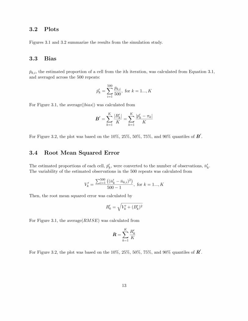
3.2 Plots

Figures 3.1 and 3.2 summarize the results from the simulation study.

3.3 Bias

pk,i, the estimated proportion of a cell from the ith iteration, was calculated from Equation 3.1,and averaged across the 500 repeats:

p′k =

500∑i=1

pk,i500

, for k = 1...,K

For Figure 3.1, the average(|bias|) was calculated from

B′=

K∑k=1

|B′k|K

=

K∑k=1

|p′k − πk|K

For Figure 3.2, the plot was based on the 10%, 25%, 50%, 75%, and 90% quantiles of B′.

3.4 Root Mean Squared Error

The estimated proportions of each cell, p′k, were converted to the number of observations, n′k.The variability of the estimated observations in the 500 repeats was calculated from

V ′k =

∑500i=1

((n′k − nk,i)2

)500− 1

, for k = 1...,K

Then, the root mean squared error was calculated by

R′k =√V ′k + (B′k)

2

For Figure 3.1, the average(RMSE) was calculated from

R =K∑k=1

R′kK

For Figure 3.2, the plot was based on the 10%, 25%, 50%, 75%, and 90% quantiles of R′.

13

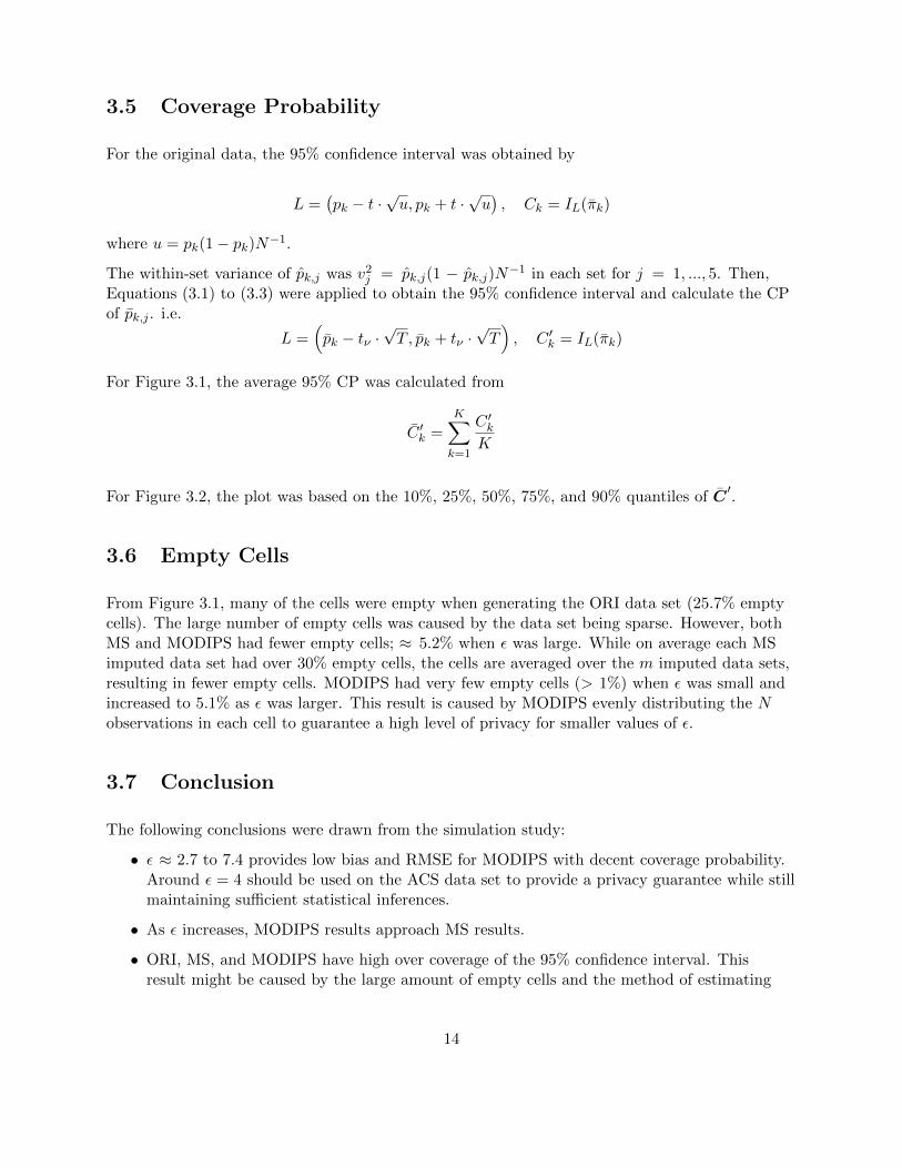
3.5 Coverage Probability

For the original data, the 95% confidence interval was obtained by

L =(pk − t ·

√u, pk + t ·

√u), Ck = IL(πk)

where u = pk(1− pk)N−1.

The within-set variance of pk,j was v2j = pk,j(1 − pk,j)N−1 in each set for j = 1, ..., 5. Then,

Equations (3.1) to (3.3) were applied to obtain the 95% confidence interval and calculate the CPof pk,j . i.e.

L =(pk − tν ·

√T , pk + tν ·

√T), C ′k = IL(πk)

For Figure 3.1, the average 95% CP was calculated from

C ′k =

K∑k=1

C ′kK

For Figure 3.2, the plot was based on the 10%, 25%, 50%, 75%, and 90% quantiles of C′.

3.6 Empty Cells

From Figure 3.1, many of the cells were empty when generating the ORI data set (25.7% emptycells). The large number of empty cells was caused by the data set being sparse. However, bothMS and MODIPS had fewer empty cells; ≈ 5.2% when ε was large. While on average each MSimputed data set had over 30% empty cells, the cells are averaged over the m imputed data sets,resulting in fewer empty cells. MODIPS had very few empty cells (> 1%) when ε was small andincreased to 5.1% as ε was larger. This result is caused by MODIPS evenly distributing the Nobservations in each cell to guarantee a high level of privacy for smaller values of ε.

3.7 Conclusion

The following conclusions were drawn from the simulation study:

• ε ≈ 2.7 to 7.4 provides low bias and RMSE for MODIPS with decent coverage probability.Around ε = 4 should be used on the ACS data set to provide a privacy guarantee while stillmaintaining sufficient statistical inferences.

• As ε increases, MODIPS results approach MS results.

• ORI, MS, and MODIPS have high over coverage of the 95% confidence interval. Thisresult might be caused by the large amount of empty cells and the method of estimating

14

the 95% confidence interval does not account for it. However, since the over estimationextends to the original data, the method that constructed the confidence interval may beinappropriate for this data set.

• Future research needs to be conducted on how the inference changes with different priorsfor MS and MODIPS (non-informative priors) and on a full mixture data set (bothcontinuous and categorical).

15

Column

#Name

Deta

ils

Num.or

Values

Rangeor

Notes

Char.

#ofClasses

1C

ITC

itiz

ensh

ipC

har

.1,

2,3,

4,5

5

2H

ISH

isp

anic

Ori

gin

Ch

ar.

1,2,

3,4,

5,6

6

3M

AR

Mar

ital

Sta

tus

Ch

ar.

1,2,

3,4,

55

4M

ILS

erve

din

Arm

edF

orce

sC

har

.1,

2,3,

44

5O

CC

Occ

up

atio

nC

od

eC

har

.1

-14

14

6O

IO

ther

Inco

me

Am

ount

Nu

m.

0-

800

99.9

9%

are

0’s

7P

OB

Pla

ceof

Bir

thC

har

.1

-21

21

8R

ET

Ret

irem

ent

Inco

me

Nu

m.

0-

800

99.9

9%

are

0’s

9S

CH

LE

du

cati

onal

Att

ain

men

tC

har

.1

-6

6

10S

EM

Sel

f-E

mp

loym

ent

Inco

me

Nu

m.

0-

800

99.9

9%

are

0’s

11S

EX

Gen

der

Ch

ar.

1,2

2

12S

SS

oci

alS

ecu

rity

orR

ailr

oad

Nu

m.

0-

800

99.9

9%

are

0’s

Ret

irem

ent

Inco

me

13A

TI

Ad

just

edT

otal

Inco

me

Nu

m.

0-

1,01

6,168

All

Inco

mes

an

dW

age

6.1

6%

are

0’s

14A

WA

GA

dju

sted

Wag

es/S

alar

yIn

com

eN

um

.0

-1,

016,

167

7.5

4%

are

0’s

15H

ICO

VA

ny

Hea

lth

Insu

ran

ceC

over

age

Ch

ar.

1,2

2

16P

OV

InP

over

tyC

har

.0,

12

17C

AG

EC

alcu

late

dA

geC

har

.1

-10

10

18V

ET

ST

AT

Vet

eran

Sta

tus

Ch

ar.

1,2,

33

19H

HT

Hou

seH

old

Fam

ily

Typ

eC

har

.1

-7

7

Tabl

e3.1

:S

um

mary

of

all

the

vari

abl

esu

nder

con

sider

ati

on

.

16

Fig

ure

3.1

:S

tati

stic

al

infe

ren

ces

of

the

ave

rage

ofπk

fork

=1,...,K

.

17

Fig

ure

3.2

:S

tati

stic

al

infe

ren

ces

ofπk

fork

=1,...,K

,plo

ttin

gth

e10%

,25%

,50%

,75%

,an

d90%

quan

tile

s.

18

Appendix A

NSF GRIP Overview

Summary of the original NSF GRIP Proposal that was submitted December 4th, 2015 by thefellow and approved March 8th, 2016 by the NSF GRIP and the US Census Bureau.

A.1 NSF GRIP Proposal

A.1.1 Overview

The fellow proposes to intern at the U.S. Census Bureau and utilize their expertise and data infurther developing current methodology in statistical disclosure limitation (SDL), i.e. methodsof data privacy and confidentiality. Specifically, the fellow will investigate SDL techniques thatpreserve differential privacy — a condition on data-releasing algorithms that quantifies disclosurerisk — such as the model-based differentially private data synthesis (MODIPS) (Bowen and Liu,2016). This project will complete the fellow’s thesis, which focuses on developing and validatingMODIPS, by providing a case study that verifies the practical applications of MODIPS inreal-world scenarios.

Intellectual Merit

The proposed project will expand the applications of differentially private data synthesis toreal-world data sets by using an innovative method, modips. To the fellow’s knowledge, thereis only one application of differentially private data synthesis on US Census Data — OnTheMap,which uses U.S. Census Bureau commuter data (Machanavajjhala et al., 2008). With the U.S.Census Bureau’s large collection of real-world data sets, the fellow will conduct case studies ofincomparable precision and contemporary relevance. The fellow is fluent in R and experienced inapplying differentially private data synthesis techniques.

Broader Impacts

Many entities such as statistical agencies, national security agencies, hospitals, and educationalinstitutions will directly benefit from the proposed project by being able to share their data

19

safely with collaborators and strike a balance between the privacy of the respondents and theefficiency and validity of the statistical inference. The U.S. Census Bureau “shares its expertiseglobally, and conducts work openly.” (U.S. Census Bureau’s mission statement).

20

A.1.2 Research Proposal

Background

In the era of information and technology, big data offers tremendous benefits for economics,national security, and other areas through data-driven decision making, insight discovery,and process optimization. However, a crucial concern is the extreme risk of exposing personalinformation of those who contribute to the data when sharing it among collaborators or releasingit publicly. An intruder could identify a participant by isolating the numerous connections toother contributors within the data set or linking to other public data sets — even with identifierssuch as name and address removed. Some examples of identification breach include the genotypeand HapMap linkage effort (Homer et al., 2008), the AOL search log release (Gotz et al., 2012),and the Washington State health record (Sweeney, 2013).

Statisticians address privacy and confidentiality issues using statistical disclosure limitation(SDL). These techniques aim to provide a high level of privacy while minimizing information lossfrom data perturbation, thus allowing valid and integrated statistical analysis for public release.One SDL method is data synthesis, which generates a synthetic data set based on the model ofthe original data (Rubin, 1993; Little, 1993; Drechsler and Reiter, 2011; Drechsler, 2011).

However, the evaluation of disclosure risk on SDL methods often depends on the specific valuesin a given data set, as well as various assumptions regarding the background knowledge andbehaviors of data intruders (McClure and Reiter, 2012; Manrique-Vallier and Reiter, 2012; Kimet al., 2015). One way to quantify disclosure risk without many such assumptions or limitationsto a specific method is differential privacy (DP) (Dwork et al., 2006; Dwork, 2008, 2011). DP wasoriginally developed for releasing summary statistics through queries submitted to a database,known as interactive privacy mechanism or query-based method.

Combining data synthesis and DP, Machanavajjhala et al. (2008) developed a differentiallyprivate mechanism, called OnTheMap, for worker commuter patterns data collected from variousUnited States Census Bureau’s data sets. The released synthetic data set shows points on a mapthat represent the commuting pattern of individuals from origin to destination within the US.Currently, OnTheMap is the only implementation of DP at the US Census Bureau.

Proposed Research Topic

U.S. Census Broad Topic: Simulation and Statistical ModelingThe fellow will investigate noise infusion for statistical disclosure control by applying variousdifferentially private data synthesis techniques, including the fellow’s model-based differentiallyprivate data synthesis (MODIPS), to real-world data sets (Bowen and Liu, 2016).

21

Appendix B

NSF GRIP Professional Developmentand Research

Summary of the fellow’s goals:

1. to implement model-based differentially private data synthesis (MODIPS – a differentialprivacy method that generates a synthetic data set) on a real-world data set

2. to include some of the research conducted at the US Census Bureau to the fellow’sdissertation as a case study

3. to establish collaborations for long-term projects at the US Census Bureau

4. to attend US Census Seminars, learning current research at the US Census

5. to connect with other scientists for potential future collaborations

The fellow accomplished the goals by:

1. implementing MODIPS on a real-world data set (but only on discrete data)

2. including the research into the fellow’s dissertation as an example application of MODIPS

3. meeting with several researchers at US Census Bureau and will continue communicationwell after the internship

4. attending over a dozen seminars during the internship, such as how LiDAR improvesspatial statistics and what current data privacy methods are applied at Google

5. connecting with other scientists such as Dr. Daniel Kifer, Professor of Computer Scienceand Engineering at Pennsylvania State University, and Dr. Jerry Reiter, Professor ofStatistics at Duke University.

22

B.1 Research Products

B.1.1 Dissertation

The fellow will incorporate the results from the internship into her dissertation as an example ofa real-world application of MODIPS.

B.1.2 Research Presentations

The fellow will present some of the findings at conferences such as the Joint Statistical Meetings,the largest international statistics conference.

Dr. Bimal Sinha invited the fellow to present her dissertation work at the University of Maryland- Baltimore County.

B.1.3 Collaborative Research

The fellow will be working with Dr. Daniel Kifer on applying differentially private data synthesistechniques on other US Census Bureau data.

B.2 Professional Development

The fellow accomplished the following professional development activities:

B.2.1 Expanded Professional Networks

The fellow met with several scientists from the Center for Statistical Research and MethodologyGroup and data privacy community at the US Census Bureau:

• Dr. John Abowd, Associate Director of Research and Methodology and Chief Scientist

• Dr. Aref Dajani, Principal Researcher at the Center for Disclosure Avoidance Research

• Dr. Maria M. Garcia, Research Mathematical Statistician at the Center for StatisticalResearch and Methodology

• Dr. Daniel Kifer, Professor of Computer Science and Engineering at Pennsylvania StateUniversity

• Dr. Martin Klein, Principal Researcher at the Center for Statistical Research andMethodology

• Dr. Amy Lauger, Principal Researcher at the Center for Disclosure Avoidance Research

23

• Laura McKenna, Special Assistant to the Associate Director for Research and Methodologyand Chair of the Disclosure Review Board

• Edward Porter, Researcher at the Center for Statistical Research and Methodology

• Dr. Jerry Reiter, Professor of Statistics at Duke University.

• Chad Russel, IT Specialist, Center for Statistical Research and Methodology

• Dr. Kimberly Sellers, Associate Professor in the Department of Mathematics and Statisticsat Georgetown University and Principal Researcher, Center for Statistical Research andMethodology

• Dr. Bimal Sinha, Professor of Statistics at the University of Maryland - Baltimore Countyand Principal Researcher, Research Mathematical Statistician at the Center for StatisticalResearch and Methodology

• Dr. Tommy Wright, Chief of the Center for Statistical Research and Methodology

The fellow also networked outside of data privacy community in the Washington D.C. area byattending the NSF Division of Graduate Education Panel at the NSF headquarterss:

• Dr. Susan E. Brennan, Program Director, NSF Division of Graduate Education

• Dr. Erik Jones, NSF GRIP Director

• Dr. Joerg Schlatterer, NSF GROW Director

• Dr. Maya Wei-Haas, Assistant Editor at the Smithsonian, resulting in an invitationto speak at the fellow’s university for the Regional Women in Science Conference(http://awis.nd.edu/wsc/).

B.2.2 Presentation

The fellow presented the concept of differential privacy to the Center for Statistical Researchand Methodology September Group meeting, improving the group’s understanding of differentialprivacy as the US Census Bureau moves toward on applying the differential privacy.

B.2.3 Communication Skills

The fellow met with several scientists at the US Census Bureau, improving verbal and writtencommunication skills.

24

Bibliography

Abowd, J. M. and Vilhuber, L. (2008). How protective are synthetic data? In Privacy inStatistical Databases, pages 239–246. Springer.

Bowen, C. M. and Liu, F. (2016). Differentially private data synthesis methods. arXiv preprintarXiv:1602.01063.

Drechsler, J. (2011). Synthetic datasets for Statistical Disclosure Control. Springer, New York.

Drechsler, J. and Reiter, J. P. (2011). An empirical evaluation of easily implemented,nonparametric methods for generating synthetic data sets. Computational Statistics and DataAnalysis, 55(12):461–468.

Dwork, C. (2008). Differential privacy: A survey of results. Theory and Applications of Models ofComputation, 4978:1–19.

Dwork, C. (2011). Differential privacy. In Encyclopedia of Cryptography and Security, pages338–340. Springer.

Dwork, C., McSherry, F., Nissim, K., and Smith, A. (2006). Calibrating noise to sensitivity inprivate data analysis. In Theory of cryptography, pages 265–284. Springer.

Gotz, M., Machanavajjhala, A., Wang, G., Xiao, X., and Gehrke, J. (2012). Publishing searchlogs - a comparative study of privacy guarantees. IEEE Trans. Knowl. Data Eng., 24:5205325.

Homer, N., Szelinger, S., Redmann, M., Duggan, D., Tembe, W., Muehling, J., Pearson, J.,Stephan, D., Nelson, S., and Craig, D. (2008). Resolving individuals contributing trace amountsof dna to highly complex mixtures using high-density snp genotyping microarrays. PLoS Genet,4(8):e1000167.

Kim, H. J., Karr, A. F., and Reiter, J. P. (2015). Statistical disclosure limitation in the presenceof edit rules.

Little, R. (1993). Statistical analysis of masked data. Journal of the Official Statistics, 9:407–407.

Liu, F. (2016). Model-based differential private data synthesis. arXiv preprint arXiv:1606.08052.

Machanavajjhala, A., Kifer, D., Abowd, J., Gehrke, J., and Vilhuber, L. (2008). Privacy: Theorymeets practice on the map. In Data Engineering, 2008. ICDE 2008. IEEE 24th InternationalConference on, pages 277–286. IEEE.

25

Manrique-Vallier, D. and Reiter, J. P. (2012). Estimating identification disclosure risk usingmixed membership models. Journal of the American Statistical Association, 107(500):1385–1394.

McClure, D. R. and Reiter, J. P. (2012). Towards providing automated feedback on the qualityof inferences from synthetic datasets. Journal of Privacy and Confidentiality, 4(1):8.

Reiter, J. P. (2003). Inference for partially synthetic, public use microdata sets. SurveyMethodology, 29(2):181–188.

Rubin, D. B. (1993). Statistical disclosure limitation. Journal of official Statistics, 9(2):461–468.

Sweeney, L. (2013). Matching known patients to health records in washington state data.Available at SSRN 2289850.

Wasserman, L. and Zhou, S. (2010). A statistical framework for differential privacy. Journal ofthe American Statistical Association, 105(489):375–389.

26