Economic Research Southern Africa (ERSA) is a research programme funded by the National

Treasury of South Africa. The views expressed are those of the author(s) and do not necessarily represent those of the funder, ERSA or the author’s affiliated

institution(s). ERSA shall not be liable to any person for inaccurate information or opinions contained herein.

Nowcasting Real GDP growth in South

Africa

Alain Kabundi, Elmarie Nel and Franz Ruch

ERSA working paper 581

February 2016

Nowcasting Real GDP growth in South Africa�

Alain Kabundi y Elmarie Nel z Franz Ruch x

February 2, 2016

Abstract

This paper uses nowcasting to forecast real GDP growth in South Africa from

2010Q1 to 2014Q3 in real time. Such an approach exploits the �ow of high-

frequency information underlying the state of the economy. It overcomes one of

the major challenges faced by forecasters, policymakers, and economic agents -

having a clear view of the state of the economy in real time. This is often not the

case as many economic variables are only available at low frequency and with con-

siderable lags, making it di¢ cult to have information on the state of the economy

even after the end of the quarter. The pseudo out-of-sample forecasts show that

the nowcasting model�s performance is comparable to those of professional fore-

casters even though the latter enhance their forecasting accuracy with judgement.

The nowcast model also outperforms all other benchmark models by a signi�cant

margin.

JEL Classi�cation Numbers: E52; C53; C33.

Keywords: Nowcasting, Factor Model, Bayesian VAR, Forecasting.

�The views expressed in this Discussion Paper are those of the author(s) and do not necessarily

represent those of the South African Reserve Bank or South African Reserve Bank policy. While every

precaution is taken to ensure the accuracy of information, the South African Reserve Bank shall not be

liable to any person for inaccurate information, omissions or opinions contained herein. We are grateful

to Shaista Amod, Chris Loewald, and Jean-François Mercier for their comments.yCorresponding author. South African Reserve Bank, PO Box 427, Pretoria, South Africa, 0001.

Email: alain.kabundi@resbank.co.za. University of Johannesburg. Economic Research Southern Africa.zSouth African Reserve Bank, PO Box 427, Pretoria, South Africa, 0001. Email: el-

marie.nel@resbank.co.za.xSouth African Reserve Bank, PO Box 427, Pretoria, South Africa, 0001. Email:

franz.ruch@resbank.co.za.

1

1 Introduction

One of the major challenges facing forecasters, policymakers, and economic agents is

having a clear view of the state of the economy in real time. As real gross domestic

product (GDP) is only available at quarterly frequency and with a signi�cant delay, it is

di¢ cult to have information on the state of the economy even after the particular quarter

has passed. For example, the fourth quarter GDP �gure for South Africa only becomes

available eight weeks after the end of the quarter. This obstructs analysis and thus

policy decisions, both of which require real-time information. However, a substantial

amount of higher frequency economic information is released between the start of the

quarter and the release of the o¢ cial GDP �gure. Although rarely exploited in growth

models, these high frequency data can help predict the current state of the economy, the

near future, and near past. This is done using nowcasting.

Nowcasting, as introduced by Giannone, Reichlin, and Small (2008), provides a

framework for the integration of a large number of timely economic series that mat-

ter for economic growth in a mixed frequency and asynchronised environment. The

prediction of the current state of the economy is known as nowcast and the prediction of

the near past as backcast. Such statistical models outperform a naïve constant growth

model in forecasting GDP growth at very short horizons, i.e. the current state and the

near future; however, they perform more poorly in the medium to long term (Giannone,

Reichlin, and Small, 2008; Banbura, Giannone, and Reichlin, 2011; Banbura, Giannone,

Modugno, and Reichlin, 2012).

So far there has been few attempts at estimating a nowcast model in Africa, let

alone for South Africa. This paper bridges the gap in the literature by estimating a

nowcast model of real GDP growth in South Africa. It uses 21 indicators covering the

real economy, nominal variables, and the �nancial sector. Like most nowcasting models,

the dataset contains variables published at di¤erent frequencies: daily, monthly, and

quarterly. Furthermore, information �ows are asynchronous resulting in missing data

toward the end of the sample with the forecasting exercise performed on the 15th of

each month. The sample period is from 2005 to 2014, while the pseudo out-of-sample

period is from 2010Q1 to 2014Q3.

We compare the performance of our nowcasting model to consensus forecasts by

Reuters and Bloomberg as well as to seven alternative models. The nowcasting model

performs similarly to consensus forecasts despite the atheoretic nature of the nowcast

approach. In contrast to the survey forecasts, our model does not incorporate judgement.

2

This becomes evident when we consider the �rst quarter of 2014 when a prolonged strike

in the platinum sector resulted in a contraction in real GDP growth. However, this does

not mean judgement can�t be incorporated after the model has evaluated the data. In

fact, the model helps disaggregate the drivers of growth assisting the forecaster to apply

judgement if needs be. The seven alternative models comprise of a random walk model,

two autoregressive (AR) models, two small-scale vector autoregressive (VAR) models,

and two large-scale VAR models. Importantly, the nowcast model outperforms all of

these models by a signi�cant margin.

The rest of the paper is organised as follows: Section 2 describes the literature and

methodological issues around nowcasting. Section 3 describes the nowcast model. We

discuss the data used in Section 4. In addition, we discuss the approach used to select the

factors and their identi�cation. Section 5 discusses the results of pseudo out-of-sample

forecasting. Section 6 provides some concluding remarks.

2 Literature Review

Giannone, Reichlin, and Small (2008) propose an approach that uses factor analysis

in a data-rich environment together with the Kalman �lter as a comprehensive and

powerful technique for forecasting the near past, the current state, and the near future

of GDP growth rate in the US. There are important �ndings from their analysis. First,

the nowcast model outperforms the naïve constant growth model over the short-run,

especially for the current quarter. Second, the proposed model performs equally well as

the professional forecasts, despite the fact that the latter includes judgement. Third, as

one would intuitively expect, the performance of the nowcast model improves as new

information becomes available and towards the end of the quarter. This means that the

forecaster can incorporate information progressively upon its release and increase their

understanding of the drivers of GDP growth. Finally, it is not necessarily the strength of

the relationship between each variable and GDP which matters, but rather the timeliness

of each variable. For example, when Purchasing Managers�Index (PMI) is released at

the beginning of each month, there is no hard data available. In addition, the Bureau of

Economic Research (BER) and the South African Chamber of Commerce and Industry

(SACCI) con�dence indices of the corresponding quarter are published respectively four

and two weeks before the end of the quarter. It implies that soft data are extremely

important (see Kabundi, 2004 and Martinsen et al., 2014).

Since the seminal work by Giannone, Reichlin, and Small (2008) there has been an

increase in popularity of these models for predicting di¤erent macroeconomic variables

and in di¤erent countries. This methodology has since been introduced in various central

3

banks such as the Federal Reserve Bank of Atlanta (2014) and the European Central

Bank (2008). There are also several applications in di¤erent countries.1 Additionally,

since the model is purely data-driven it allows an array of innovative practices. Instead of

using key determinants of GDP, Angelini, Banbura, and Runstler (2010) forecast di¤er-

ent components of GDP, and then aggregate them to obtain a nowcast of GDP. Another

variation of the technique is Liebermann (2012), who provides a detailed study on the

nowcasting of a large variety of key monthly macroeconomic releases, while Modugno

(2013) uses the same framework for forecasting in�ation.

Nowcasting ensures �exibility by overcoming three common challenges. First, given

that data is released in di¤erent frequencies, the forecaster needs to reconcile the data

into a single frequency. For example, manufacturing production, which is closely related

to GDP, is published monthly. The problem of mixed-frequency is easily translated

to a task of missing data. Traditionally, forecasters use bridge equations as means of

reconciling mixed-frequency information. However, such a solution is suboptimal, as

bridge equations are single regression models that can only accommodate few variables.

Second, data are not released in a synchronous fashion. For example, the PMI

for February is published at the beginning of March, while the exports and imports

for February become available at the end of March. Similar to the mixed-frequency

problem, the unbalanced panel at the end of the period is also looked at as a missing-

data question. One way of solving this problem is to move all series later in order to have

a balanced panel at the end of the period. The drawback of such approach is one does

not take into account the true contemporaneous correlation that exists among variables

at each period introducing a lead-lag relationship between variables. Evans (2005) and

Giannone, Reichlin, and Small (2008) propose the use of the Kalman �lter as a solution

to this problem, given its ability to adapt to changing data availability.

This leads to the third challenge - most traditional models are unable to accom-

modate a large set of information. Nowcasting overcomes the curse of dimensionality

(large number of parameters relative to the number of observations) by summarizing

information using a dynamic factor model. Meaning that forecasters bene�t from a

1Kuzin, Marcellino, and Schumacher (2013) use model combination in nowcasting the German GDP,

Matheson (2010) nowcasts New Zealand GDP and CPI, Yiu and Chow (2011) and Giannone, Agrippino,

and Modugno (2013) use it for China, Aastveit and Trovik (2008) build a nowcast model for Norway,

Siliverstovs and Kholodilin (2010) apply the same approach for Switzerland, D�Agostino, McQuinn, and

O�Brien (2008) for Ireland, Barhoumi, Darn and Ferrara (2010) nowcast the French GDP growth, de

Winter (2011) shows the superiority of this technique for the Netherlands, Arnostova, Havrlant, Ruzicka

and Toth (2011) con�rms the �ndings by other scholars for the Czech Republic, and for Brazil Bragoli,

Metelli, and Modugno (2014) show that nowcasting performs as well as predictions of professional

forecasters. Matheson (2011) tracks growth in 32 advanced and emerging-market economies with a

nowcast.

4

rich information set. Forni, Hallin, Lippi, and Reichlin (2003) and Stock and Watson

(2003) demonstrated that factor models turn the curse of dimensionality into a blessing

of dimensionality.

3 The Nowcasting Model

The added advantage from nowcasting is its ability to use high frequency data (daily

and monthly in our case) to estimate quarterly macroeconomic variables. Thus we

estimate GDP in quarter q, zqkj�j , by using the information available during that quarter,

denominated as �j . We estimate

zqkj�j = Proj[zqkjj ] (1)

As more information is released, this is integrated into the projection. Thus the

forecast is made with the most up-to-date and comprehensive information set at each

point in time such that

�j > �j�1 > �j�2 > ::: (2)

We estimate GDP using the dynamic factor model suggested by Doz, Giannone and

Reichlin (2005). Since the frequency of the dataset di¤ers, introducing missing data

points, and the common factors are unobserved, we need to use the Kalman �lter. The

Kalman �lter is a discrete, recursive linear �lter used to estimate unobservable variables

in a system of equations given an information set (Pasricha, 2006). The Kalman �lter is

optimal because it minimises the mean squared error estimator, if the observed variable

and error are jointly Gaussian and is �best�in the class linear �lters if this assumption

is violated.

The factor, Ft, summarises the co-movements from the latest available information

set. Thus we estimate the corresponding monthly GDP, ytj�j , to the quarterly series zqkj�j

by

ytj�j = �+ �Ft + �tj�j (3)

where � is a constant, � is r �m coe¢ cient matrix, �tj�j is a white noise error, and Ftis the unobserved factor. We specify the common factors as VAR(1)

Ft =MFt�1 +N�t (4)

where M is a r � r matrix, N is a r � l matrix of full rank r and �t the common factorshocks.

5

As there can be more than one signi�cant co-movement in the information set, there

can be more than one factor needed in the model. We test the number of common factors

using the modi�ed Bai and Ng (2002) information criterion.2 To determine the number

of common factors, this method determines the factor which minimises the variance of

the idiosyncratic component.3

Near-term forecasting rarely provides any insight to the marginal change in GDP.

This is not the case with nowcasting. Since the model is purely data-driven it permits

the breakdown of the marginal impact of speci�c variables on the GDP forecast, making

it possible to analyse the drivers of the forecast. This ability is called the News of the

model.

We estimate the News by

NEWS[zqkj�j ; �j] = zqkj�j � z

qkj�j�1 (5)

which is the di¤erence between the forecast of GDP including zqkj�j and excluding zqkj�j�1

the most recent datapoint of various variables used. Thus, indicating the impact of

certain datapoints on GDP. This is a valuable function as the impact of recent releases

can pinpoint latest developments in the economy and increase our understanding of the

current state of the economy.

4 Alternative Models

We use �ve alternative models which serve to compare the performance of the nowcasting

model. Unlike the nowcasting model which uses data in mixed-frequency domain, the

alternative models use only quarterly variables. We use a combination of univariate and

multivariate models. The univariate models include the random walk (RW) model and

the autoregressive model of the form

Yt = B0 +B1Yt�1 +B2Yt�2 + :::+BpYt�p + �t (6)

where �t is the error term. Equation 6 is a RW with drift when B1 = 1; B0 6= 0, and

the coe¢ cients of other lags are set to zero. However, if B0 = 0, the model is RW

without drift. Equation 6 is an autoregressive process of order p when the coe¢ cients

of Yt�1; Yt�2; :::; Yt�p are di¤erent from zero. The paper uses two autoregressive models,

namely, AR(1) and AR(4). If Yt is a vector, Equation 6 becomes a multivariate model

known as Vector Autoregressive (VAR) model. The estimation procedure includes four

2As proposed by Alessi, Barigozzi and Capasso (2010).3For more detail on the test speci�cations see Alessi, Barigozzi and Capasso (2010).

6

VAR models, two small-scale VARs and two large-scale VARs. The small-scale VARs

contain four variables, namely, GDP growth, CPI in�ation, the repo rate, and the nom-

inal e¤ect exchange rate. We use both VAR(1) and VAR(4) for small-scale VAR.

Given that the nowcasting model comprises 21 variables, it is appropriate to compare

its forecasting performance with other large-scale models. But the traditional VAR

models cannot accommodate such large number of variables without facing the degree-

of-freedom issue, which in turn a¤ects negatively the forecasting performance of the

model. The main reason underlying poor performance of large VARs is the uncertainty

concerning parameter estimation. Recently Gupta and Kabundi (2011) show that large-

scale outperform small-scale models in forecasting GDP growth for South Africa. Thus,

in addition to small-VARs we use a Factor-Augmented VAR (FAVAR) and a Large

Bayesian VAR (LBAVAR) as alternative models. The FAVAR adds two common factors

obtained from a panel of 17 of 21 variables included in the nowcasting model to four

variables used in the small-scale VARs. The extracted factors summarise the information

contained in the panel of 17 variables. Hence, instead of estimating a VAR with 21

variables, we estimate a VAR with six variables, four observed and two unobserved. The

common factors are estimated using the VAR(1) as speci�ed in Equation (3).

The LBVAR solves the problem of overparameterisation by shrinking parameters

towards a parsimonious naïve random walk process using informative priors. Giannone,

Lenza, and Primiceri (2015) demonstrate the superiority of these models in out-of-sample

forecasting as they reduce the uncertainty associated with the estimation based �at pri-

ors when the number of variables increases signi�cantly. However, the BVARs models

are highly dependent on the choice of priors. Many empirical studies in economics use

the Minnesota priors which shrink the parameters towards a random walk process.4

The main issue with the Minnesota priors is the subjectivity it involves in the choice of

priors. Instead this paper follows recent development by estimating prior hyperparame-

ters as proposed by Giannone, Lenza, and Primiceri (2015). These authors treat these

hyperparameters as additional parameters that need to be estimated.5

5 Data

The dataset contains 21 series covering real variables, nominal variables, and �nancial

variables.6 Giannone, Reichlin, and Small (2008) show that if variables are selected

4See for example Kadiyala and Karlsson (1997), Banbura, Giannone, and Reichlin (2010).5We refer to Giannone, Lenza, and Primiceri (2015) for a technical explanation of LBVAR.6Table 1 provides a complete list of variables. In addition, it shows the treatment, the source, the

frequency, and the Bloomberg relevance of all variables.

7

systematically including timely information concerning the current state of the economy,

the cross-section need not to be very large. The real sector includes trade, production,

and demand variables. The nominal variables are producer and consumer price indices,

and the Brent crude oil price (in US dollar). Financial variables are the nominal e¤ective

exchange rate and the policy rate (repurchase rate). Most series are expressed in log

di¤erenced at the monthly frequency.

Table 1: List of VariablesVariables Sources Frequency Lag* Relevance Treatment**Nominal Effective Exchange Rate SARB D 0 5Kagiso Purchasing Manager Index BER M 1 70.27 1Total Retail Trade Sales STATS SA M 44 64.86 5Real Wholesale Trade Sales STATS SA M 46 0.00 5Mining Production STATS SA M 44 27.73 5Private Credit SARB M 29 51.35 1Electricity Consumption STATS SA M 39 10.81 5Motor Vehicle Sales NAAMSA M 2 32.43 5SACCI Business Confidence SACCI M 3 54.05 5Exports SARS M 31 94.59 5Imports SARS M 31 94.59 5Money Supply M3 SARB M 29 78.38 5Oil price ­ US dollar (Brent crude) OECD M 0 5Trade Activity Index SACCI M 12 1Trade Expectations Index SACCI M 12 1Gold Production STATS SA M 44 50.00 5Business Cycle Indicator SARB M 51 24.32 5Consumer Price Index STATS SA M 20 72.97 5Producer Price Index STATS SA M 30 78.13 5Repo Rate SARB M 0 97.30 1BER Consumer Confidence BER Q ­12 67.57 1Capacity Utilisation STATS SA Q 67 0.00 1Gross Domestic Product STATS SA Q 57 62.16 5* Avergage number of days after the end of the observed period before that period's figure is released.** 1 = no transformation, 5 = first difference of logarithm,

Quarterly series used are capacity utilisation, consumer con�dence, and real GDP

growth. These series are transformed into monthly frequency with quarterly values set

as third month observations and missing data for the remaining two months of the

quarter. Then, we use the Kalman �lter to manage the missing data issue. The nominal

e¤ective exchange rate, the only variable obtained at daily frequency, is transformed

to a monthly frequency by taking average of 15 days for each month since the pseudo

real-time out-of-sample forecast exercise is conducted on the 15th of each month. All

variables are transformed to induce stationarity. For professional forecasters, we use

the forecasts based on the surveys conducted by Reuters published monthly, while the

Bloomberg forecasts are released two days before the GDP release.7

7The mean of the Reuters survey is used.

8

The �rst task in nowcasting is the choice of variables to include. We use the view of

market participants obtained from Bloomberg to decide on which variables to include.

Note that the policy rate matters more with a weight of 97.30, followed by trade balance

with 94.59. Even though PMI seems less important than trade balance, it is timely, with

only one day lag, while the latter is published with 31 days lag. Except for PMI and

con�dence indices, all variables are expressed as quarterly growth rate. In addition, we

use annual growth for vehicles sales.

Table 2: Correlation coe¢ cients

GDP PMI Retail Electricity Vehicle BCI TEIGDP 1PMI 0.80 1Retail 0.67 0.70 1Electricity 0.66 0.67 0.50 1Vehicle 0.58 0.62 0.59 0.50 1BCI 0.64 0.66 0.64 0.63 0.70 1TEI 0.67 0.76 0.65 0.71 0.68 0.65 1

Table 2 shows correlation coe¢ cients between di¤erent variables. All variables are

standardised to have the same unit of measurement. Most of the correlation coe¢ cients

are above 0.5, which is evidence that they move together. Importantly, they are highly

correlated with GDP growth. PMI is the variable that mimics GDP growth quite closely.

Even though, it is perceived as soft data, it is closely related to hard data and it is

timely. Figure 1 shows how close PMI tracks GDP. It is incredible how PMI predicts

turning points. It is mostly contemporaneous with GDP growth. It depicts a correlation

coe¢ cient of 0.8. This relatively high correlation is con�rmed in Figure 1. In addition,

Figure 2 con�rms the observation in Table 2 about relatively strong correlation among

real variables. It depicts evidence of strong co-movement with GDP growth which implies

that they can serve as its determinants. Instead of choosing one variable over another,

the model has the advantage of exploiting the data-rich information represented in Table

1. In contrast, traditional econometric models cannot accommodate all of these variables

simultaneously in one model due to over�tting. Factor analysis can.

9

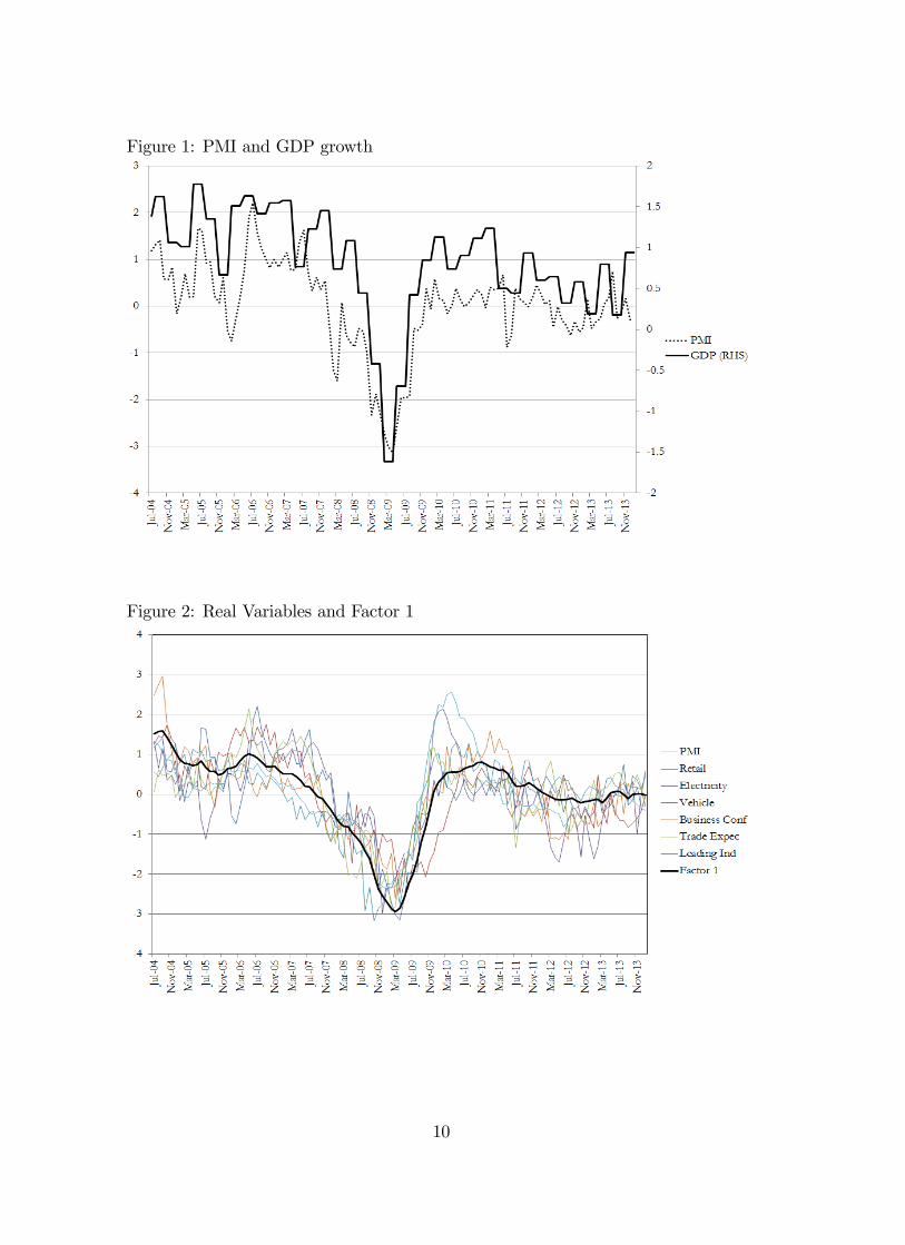
Figure 1: PMI and GDP growth

Figure 2: Real Variables and Factor 1

10

6 Empirical Results

We perform a pseudo real-time out-of-sample forecasting from the �rst quarter of 2010

to third quarter of 2014, using monthly and daily information from January 2005 to

November 2014. We conduct the forecasting on the 15th of each month. The �rst task

in nowcasting is to determine the number of factors to include. We use the Alessi,

Barigozzi, and Capasso (2010) approach, an improvement of the most popular Bai and

Ng (2002) methodology. We use one lag in the state equation for the estimation of

factors. We compare our nowcasting model to both survey results as well as some

benchmark models.

6.1 Determining the number of common factors and shocks

In order to determine the number of common factors to use in the model we implement

a modi�ed Bai and Ng (2002) information criterion as implemented by Alessi, Barigozzi

and Capasso (2010). This method chooses the number of factors by minimising the

variance of the idiosyncratic component of the approximate factor model. This is subject

to a penalisation in order to avoid over-parameterisation. The information criterion is

rTc;N = argmin0�k�rmax

ICT��;N(k) (7)

where

ICT��;N(k) = log[1

NT

NXi=1

TXi=1

(xit � (k)i F(k)t )2] + ckpa(N; T ) for a = 1; 2 (8)

For k common factors, N is the number of variables, T the number of observations,

xit � (k)i F(k)t the idiosyncratic error, c an arbitrary positive real number and pa(N; T )

the penalty function.8 Alessi et al. (2010) propose multiplying the penalty function by c

since Hallin and Liska (2007) show that a penalty function, p(N; T ), leads to consistent

estimation of r < k, the number of factors, if and only if cp(N; T ) does as well.

The only information available regarding the behaviour of rTc;N can be gleaned from

analysing subsamples of sizes (nj; tj). For any j, we can compute rtjc;nj which is a

monotonic non-increasing function in c. Therefore, there exist moderate values of c

such that rTc;N converges from above to r. This result, however, needs to be independent

of j for the criterion to be stable. This is measured by the variance of rtjc;nj as a function

of j:

8See Alessi et al. (2010) for the functional form of the penalty function.

11

Sc =1

J

JXj=1

[rtjc;nj �1

J

JXj=1

rtjc;nj ]2 (9)

Figure 3 shows the estimated number of factors for our model. The vertical axis

represents the number of factors while the horizontal axis represents an arbitrary positive

real number c. We run the results over a number of sizes for the subsamples in order to

get a robust result. In order to determine the number of factors we have to �nd the �rst

value of rtjc;nj where Sc is zero. The results suggest that the number of factors should be

two.

Figure 3: ABC criterion for common factors

The other important choice that is required in the model is the number of common

shocks, l, included. As we only use two common factors, we can easily assume that one

common shock will be su¢ cient. This is based on arguments made by Forni et al. (2005)

and Bai and Ng (2007) that the number of common shocks (l) is less than the number

of common factors (r). This argument follows as economic �uctuations are driven by a

small number of common shocks. However we test the number of common shocks using

the information criterion speci�ed by Onatski (2009). We test the null hypothesis of

l = l0 shocks versus the alternative hypothesis of l0 < l � l1 shocks. The test (Table 3)supports the arguments made by Forni et al. (2005) and Bai and Ng (2007), determining

a common shock of one.

12

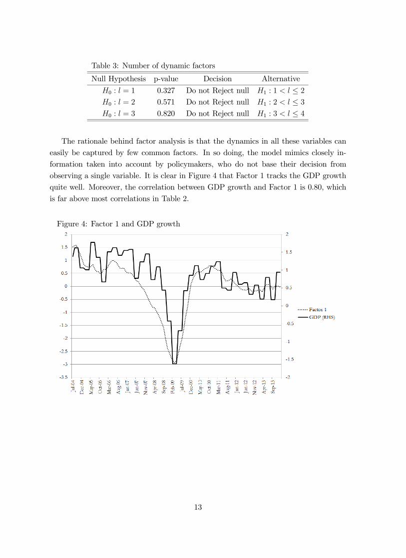
Table 3: Number of dynamic factors

Null Hypothesis p-value Decision Alternative

H0 : l = 1 0.327 Do not Reject null H1 : 1 < l � 2H0 : l = 2 0.571 Do not Reject null H1 : 2 < l � 3H0 : l = 3 0.820 Do not Reject null H1 : 3 < l � 4

The rationale behind factor analysis is that the dynamics in all these variables can

easily be captured by few common factors. In so doing, the model mimics closely in-

formation taken into account by policymakers, who do not base their decision from

observing a single variable. It is clear in Figure 4 that Factor 1 tracks the GDP growth

quite well. Moreover, the correlation between GDP growth and Factor 1 is 0.80, which

is far above most correlations in Table 2.

Figure 4: Factor 1 and GDP growth

13

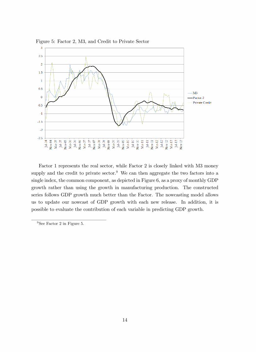
Figure 5: Factor 2, M3, and Credit to Private Sector

Factor 1 represents the real sector, while Factor 2 is closely linked with M3 money

supply and the credit to private sector.9 We can then aggregate the two factors into a

single index, the common component, as depicted in Figure 6, as a proxy of monthly GDP

growth rather than using the growth in manufacturing production. The constructed

series follows GDP growth much better than the Factor. The nowcasting model allows

us to update our nowcast of GDP growth with each new release. In addition, it is

possible to evaluate the contribution of each variable in predicting GDP growth.

9See Factor 2 in Figure 5.

14

Figure 6: Common component and GDP growth

6.2 Forecasting results

We compare our nowcasting model to both survey results as well as real-time benchmark

models. These models include:

� a random walk model (labelled RW);

� two autoregressive models with one and four lags (labelled AR(1) and AR(4));

� two four variable vector autoregressive models with one and four lags (labelledVAR(1) and VAR(4)). These models include consumer price in�ation, the repur-

chase rate and the nominal e¤ective exchange rate;

� a FAVAR model including two unobserved common factors and four observed vari-ables included in VAR(1) and VAR(4);

� and a LBVAR model including all 17 variables included in the FAVAR model.

Contrary to most nowcasting models in the literature which include manufacturing

production, we exclude this variable as it a¤ects the forecasting bias. Wholesale trade

and trade activity index portray similar e¤ects in predicting GDP growth in South

Africa. Figure 7 illustrates the negative impacts of the wholesale sale trade and the

trade activity index rendering the forecast biased upward. By including these variables

15

the model performs well in predicting the peaks, whereas it falls short in predicting the

troughs. Hence, we decide to remove them from the analysis.

Figure 7: Model with and without Wholesale Trade and Trade Activity Index

Note from Figure 7 that the GDP growth recorded in the out-of-sample period is

less stable. Figure 8 represents the results based on nowcasting and the results of the

professional forecasters based on the surveys conducted by Reuters and Bloomberg. The

results, based on forecasts made by Reuters, show an upward biased in forecasting. In

general they tend to predict relatively well the peaks, but they miss the troughs. Nev-

ertheless it is worth mentioning the di¢ culty faced by forecasters in predicting turning

points. However, forecasts by Bloomberg follow closely the real-time GDP growth.

16

Figure 8: Nowcast vs Professional Forecasters

Figures 9 and 10 depict out-of-sample forecasts of alternative models, namely, AR(1),

VAR(1), FAVAR, and LBVAR. All these models forecasts GDP growth with one lag.

They display the same pattern since 2013Q1. Interestingly, they all miss the contraction

of �rst quarter of 2014 by a considerable amount. We attribute the superiority of the

nowcast model to the bene�t it incurs from real-time �ow of information. Even though

it uses relatively the same number of variables as the large-scale models, it outperforms

them by far.

17

Figure 9: Nowcast vs AR(1) and VAR(1)

Figure 10: Nowcast vs FAVAR and LBVAR

Table 4 compares the out-of-sample Root Mean Squared Forecast Errors (RMSFEs)

of the nowcast model, the two surveys, as well as the benchmark models. The results

show that both survey outcomes do better than the nowcast model with the lowest

RMSFE of 0.406 by the Bloomberg survey. The results con�rm the observation in Figure

18

8. But the superiority of Bloomberg forecasts can be attributed to its timeliness. Recall

that Bloomberg forecasts are published two days before the release of GDP. Hence, these

forecasters bene�t from most recent information which are unavailable to the nowcast

model used and the Reuters survey. The latter�s results are marginally better than the

nowcast model with a RMSFE of 1.129 versus 1.145. Importantly, however, this result

is driven by one outlier in 2014Q1. If we exclude this datapoint, the nowcast model

outperforms the Reuters survey. This is despite the fact that these surveys incorporate

judgement, a luxury the nowcast model does not have. In addition, it is evident from

Table 4 that the nowcast model outperforms all benchmark models even the large scale

models which are known to do well given the advantage they possess in accommodating

many variables and thus solving the problem of overparameterisation common with

traditional VARs.

Table 4: Out-of-sample Root Mean Squared Forecast ErrorsNowcast Bloomberg Reuters LBVAR FAVAR AR(1) AR(4) VAR(1) VAR(4) RW

2010 Q1 0.265 0.084 1.567 2.014 0.009 2.605 4.961 0.177 2.274 1.957

Q2 0.227 0.292 0.921 1.341 6.368 0.515 0.224 3.766 2.371 1.904

Q3 1.366 0.430 0.312 0.156 4.715 0.162 0.022 2.379 6.500 0.379

Q4 0.497 0.060 1.311 2.049 0.125 3.483 3.929 0.557 0.263 3.427

2011 Q1 1.392 0.483 2.087 0.256 0.004 0.940 0.510 0.000 0.514 0.160

Q2 3.537 0.082 4.734 8.489 15.591 8.400 8.510 13.288 16.837 12.820

Q3 1.739 0.124 1.566 0.095 1.718 0.043 0.016 1.050 5.409 0.034

Q4 0.527 0.004 0.201 1.469 0.582 1.894 1.406 0.592 0.195 2.947

2012 Q1 0.200 0.244 0.000 0.120 0.134 0.056 0.408 0.349 0.186 0.177

Q2 1.130 0.011 0.140 0.236 0.031 0.252 0.404 0.211 0.028 0.202

Q3 0.440 0.073 1.590 3.659 5.584 3.140 3.084 5.624 2.614 3.854

Q4 0.075 0.186 0.154 0.299 0.092 0.236 0.370 0.148 2.144 0.810

2013 Q1 1.058 0.503 2.692 1.711 2.456 1.907 2.219 2.496 4.702 1.537

Q2 0.179 0.045 0.025 3.452 2.574 2.687 2.359 1.034 0.467 4.609

Q3 2.047 0.066 2.357 5.657 7.069 4.624 5.254 6.801 3.801 5.270

Q4 2.719 0.189 1.256 7.658 5.219 6.393 6.425 4.707 3.071 9.562

2014 Q1 8.179 0.178 2.989 15.823 18.600 16.355 15.872 20.660 19.966 19.863

Q2 0.608 0.085 0.316 0.251 0.016 0.049 0.006 0.000 0.162 1.513

Q3 0.166 0.003 0.006 0.120 0.048 0.049 0.400 0.133 1.451 0.708

RMSFE (excl. 2014Q1) 1.005 0.406 1.086 1.473 1.705 1.442 1.500 1.551 1.716 1.698

RMSFE 1.178 0.407 1.129 1.699 1.932 1.683 1.723 1.835 1.960 1.943

Relative to RW 0.606 0.209 0.581 0.874 0.994 0.866 0.887 0.944 1.008 1.000

19

7 Conclusion

Real GDP growth is the single most relevant variable describing the path of the economy

and is used, together with in�ation, to substantiate the direction of the monetary policy.

Unfortunately, the GDP �gure is released with a signi�cant lag, usually between six to

eight weeks after the end of the relevant quarter. The proposed framework allows us to

overcome this problem by exploiting valuable high frequency data to forecast real GDP.

The framework uses a dynamic factor model to summarise this dataset providing

a nowcast of current quarter growth from 2010 to 2014. Furthermore it provides a

mechanism to determine the marginal impact of new data releases on real GDP growth.

The bene�t of this marginal impact or news is that a forecaster can quantify the evolution

of economic activity in real time. Also it provides policymakers with the likely meaning

of a large number of economic series on the path of real economic activity.

Given the relatively short period of real-time data, the results should be interpreted

with caution with further monitoring required. Nevertheless, the results shows that

this model performs comparatively well against consensus forecasts of quarterly growth

by Reuters. This is despite the model not incorporating judgement as is the case in

the Reuters survey. A pertinent example in South Africa occurred in the �rst quarter

of 2014 when a prolonged strike in the platinum sector resulted in a contraction in

real GDP growth, something that survey participants could adjust for but that wasn�t

fully captured in the data. Encouragingly, if you remove this data point, the nowcast

model outperforms the survey. The nowcast model also outperforms all other benchmark

models by a signi�cant margin.

20

References

[1] Alessi, L., Barigozzi, M. and Capasso, M. (2010): �Improved penalization for deter-

mining the number of factors in approximate factor models,�Statistics & Probability

Letters, 80(23-24): 1806-1813.

[2] Aastveit, K., and T. Trovik (2012): �Nowcasting norwegian GDP: the role of asset

prices in a small open economy,�Empirical Economics, 42(1): 95�119.

[3] Angelini, E., M. Banbura, and G. Runstler (2010): �Estimating and forecasting

the euro area monthly national accounts from a dynamic factor model,� OECD

Journal: Journal of Business Cycle Measurement and Analysis, 2010(1), 7.

[4] Arnostova, K., D. Havrlant, L. Ruzicka, and P. Toth (2011): �Short-Term Fore-

casting of Czech Quarterly GDP Using Monthly Indicators,�Czech Journal of Eco-

nomics and Finance, 61(6): 566�583.

[5] Bai, J. and Ng, S., (2002): �Determining the number of factors in approximate

factor models,�Econometrica, pp.191�221

[6] Banbura, M., D. Giannone, and L. Reichlin (2010). �Large Bayesian vector auto

regressions,�Journal of Applied Econometrics, 25: 71�92.

[7] Banbura, M., D. Giannone, and L. Reichlin (2011): �Nowcasting,�in Oxford Hand-

book on Economic Forecasting, ed. by M. P. Clements, and D. F. Hendry, pp. 63�90.

Oxford University Press.

[8] Banbura, M., D. Giannone, M. Modugno, and L. Reichlin (2012): �Now-Casting

and the Real-Time Data-Flow�, in G. Elliott and A. Timmermann, eds., Handbook

of Economic Forecasting, Volume 2, Elsevier-North Holland, forthcoming.

[9] Barhoumi, K., O. Darn, and L. Ferrara (2010): �Are disaggregate data useful for

factor analysis in forecasting French GDP?,�Journal of Forecasting, 29(1-2): 132�

144.

[10] Bragoli, D., Metelli, L., and Modugno, M. (2014): �The Importance of Updating:

Evidence from a Brazilian Nowcasting Model,�Discussion Series 2014-94, Board of

Governors of the Federal Reserve System

[11] D�Agostino, A., K. McQuinn, and D. O�Brien (2008): �Now-casting Irish GDP,�

Research Technical Papers 9/RT/08, Central Bank & Financial Services Authority

of Ireland (CBFSAI).

21

[12] de Winter, J. (2011): �Forecasting GDP growth in times of crisis: private sector

forecasts versus statistical models,�DNBWorking Papers 320, Netherlands Central

Bank, Research Department.

[13] European Central Bank (2008): �Short-term forecasts of economic activity in the

euro area,�in Monthly Bulletin, April, pp. 69�74. European Central Bank.

[14] Evans, M. D. D. (2005): �Where Are We Now? Real-Time Estimates of the Macro-

economy,�International Journal of Central Banking, 1(2).

[15] Forni, M., Hallin, M., Lippi, M. and Reichli, L. (2001): �Coincident and Leading In-

dicators for the Euro Area, �Economic Journal, Royal Economic Society, 111(471):

62�85.

[16] Forni, M., M. Hallin, M. Lippi, and L. Reichlin (2003): �Do �nancial variables

help forecasting in�ation and real activity in the euro area?,�Journal of Monetary

Economics, 50(6): 1243�1255.

[17] Giannone, D., Reichlin, L., and Small, D. (2008). �Nowcasting: The real-time infor-

mational content of macroeconomic data,�Journal of Monetary Economics, 55(4):

665�676.

[18] Giannone, D., Agrippino, S.M. and Modugno, M. (2013): �Nowcasting China Real

GDP�Mimeo

[19] Giannone, D., Lenza, M., and Primiceri, G.E. (2015). �Prior Selection for Vector

Autoregressions,�Review of Economics and Statistics, 97(2): 436-451.

[20] Gupta, R. and Kabundi, A. (2011). �A Large Factor Model for Forecasting Macro-

economic Variables in South Africa�, International Journal of Forecasting, 27(4):

1076-1088.

[21] Hallin, M. and Liska, R. (2007): "Determining the number of factors in the general

dynamic factor model," Journal of the American Statistical Association, 102(478):

603�617.

[22] Kabundi, A. (2004). �Estimation of Economic Growth in France Using Business

Survey Data�, IMF Working Papers 04/69, International Monetary Fund.

[23] Kadiyala, K.R. and Karlsson, S. (1997). �Numerical methods for estimation and

inference in Bayesian VAR-models�, Journal of Applied Econometrics, 12(2): 99�

132.

22

[24] Kuzin, V., M. Marcellino, and C. Schumacher (2013): �Pooling versus Model Se-

lection for Nowcasting with Many Predictors: An Application to German GDP,�

Journal of Applied Econometrics, 28(3): 392-411.

[25] Martinsen, K., F. Ravazzolo , F. Wulfsberg (2014): �Forecasting Macroeconomic

Variables using Disaggregate Survey Data,� International Journal of Forecasting,

30(1): 65-77.

[26] Matheson, T. (2011): �New Indicators for Tracking Growth in Real Time,� IMF

Working Papers 11/43, International Monetary Fund.

[27] Matheson, T. D. (2010): �An analysis of the informational content of New Zealand

data releases: The importance of business opinion surveys,�Economic Modelling,

27(1): 304�314.

[28] Modugno, M. (2011): �Nowcasting in�ation using high frequency data,� Interna-

tional Journal of Forecasting, 29(4): 664-675.

[29] Stock, J. H., and M. W. Watson (2003): �Forecasting Output and In�ation: The

Role of Asset Prices,�Journal of Economic Literature, 41(3): 788�829.

[30] Yiu, M. S., and K. K. Chow (2010): �Nowcasting Chinese GDP: Information Con-

tent of Economic and Financial Data,�China Economic Journal, 3(3): 223�240.

23