novel injection techniques to enable fast, high peak
TRANSCRIPT

Novel Injection Techniques to Enable Fast, High Peak Capacity Gas Chromatography
Separations
Ryan Bradley Wilson
A dissertation
submitted in partial fulfillment of the
requirements for the degree of
Doctor of Philosophy
University of Washington
2012
Reading Committee:
Robert Synovec, Chair
Matthew Bush
Michael Heinekey
Program Authorized to Offer Degree:
Chemistry

UNIVERSITY OF WASHINGTON
ABSTRACT
NOVEL INJECTION TECHNIQUES TO ENABLE FAST, HIGH PEAK
CAPACITY GAS CHROMATOGRAPHY SEPARATIONS
Ryan Bradley Wilson
Chair of the Supervisory Committee:
Professor Robert E. Synovec
Department of Chemistry
To achieve faster gas chromatographic (GC) analysis of increasingly complex samples
requires improved peak capacity production (peak capacity per separation run time) from the
separation. The increased peak capacity production was achieved by selecting appropriate
experimental conditions based on theoretical modeling of on-column band broadening , by
reducing the injection pulse width, and by the implementation of a second, serially connected

column to make a GC × GC instrument. Modeling to estimate the on-column band broadening
from experimental parameters provided insight to achieving GC separations in the absence of
off-column band broadening (the additional band broadening not due to the on-column
separation process). In order to optimize separations collected on a traditional GC platform, off-
column band broadening from injection was significantly reduced by using a variety of modified
injection devices (includeing diaphragm valves, commercially available thermal modulators, and
a custom built high speed cryofocusing injector) to generate narrow pulses on the separation
column for both isothermal and temperature programmed separations. Additionally, off-column
band broadening from detection was minimized by implementation of fast detectors such as
flame ionization detectors (FID) and time-of-fligh mass spectrometry (TOFMS) collecting data
at rates greater than 500 Hz. This resulted in a 2 to 3-fold improvement in peak capacity
production compared to standard GC practice. The optimized injection techniques and separation
conditions described above were also applied to GC × GC instrumentation with both valve and
thermal modulators, resulting in 5 to 10-fold improvement in peak capacity production relative to
traditional instruments.

i
TABLE OF CONTENTS
Page
List of Figures ii
List of Tables iv
Acknowledgement v
CHAPTER 1 Introduction to Gas Chromatography 1
CHAPTER 2 Achieving High Peak Capacity Production for Gas Chromatography
and Comprehensive Two-Dimensional Gas Chromatography by
Minimizing Off-Column Peak Broadening 23
CHAPTER 3 High-Speed Cryo-Focusing Injection for Gas Chromatography:
Reduction of Injection Band Broadening with Concentration
Enrichment 42
CHAPTER 4 High Throughput Analysis of Atmospheric Volatile Organic
Compounds by Isothermal Gas Chromatography – Time-of-Flight
Mass Spectrometry 58
CHAPTER 5 Fast, High Peak Capacity Separations in Gas Chromatography –
Time-of-Flight Mass Spectrometry 78
CHAPTER 6 Conclusion 95
Bibliography 101
Curriculum Vitae 127

ii
LIST OF FIGURES
Figure 1.1 Plot of peak width at the base, Wb@opt, vs. column length, L...................................... 11
Figure 2.1 Diagram of the Agilent 6890 GC with the modified injection system ....................... 25
Figure 2.2 (A) 2D separation with transfer line (B) heated transfer line. .................................... 29
Figure 2.3 (A) Pi at ūopt vs. L (B) ūopt vs. L (C) Wb@opt vs. L. ...................................................... 31
Figure 2.4 (A) H vs. ū (B) wb vs. ū .............................................................................................. 32
Figure 2.5 Separation of four analyte text mixture with standard Agilent 6890 GC auto-
injection....................................................................................................................... 34
Figure 2.6 Separation of four analyte test mixture with modified injection system .................... 35
Figure 2.7 Rapid separation of a gasoline sample with the modified injection system ............... 37
Figure 2.8 GC x GC-FID chromatogram of test mixture ............................................................. 39
Figure 3.1 Instrument Schematic ................................................................................................. 45
Figure 3.2 Chromatogram of pentane and octane ........................................................................ 48
Figure 3.3 Plot of peak width vs. HSCFI pulse voltage ............................................................... 49
Figure 3.4 Separation of head space injection. ............................................................................ 51
Figure 3.5 Plot of peak height vs. volume of head space vapor injected. .................................... 52
Figure 3.6 Rapid separation of a gasoline sample. ...................................................................... 55
Figure 4.1 Schematic of GC – TOFMS instrument with thermal injection ................................. 64
Figure 4.2 Separation of a VOC text mixture with thermal injection .......................................... 65
Figure 4.3 Wb,t vs. k ...................................................................................................................... 69
Figure 4.4 Simulated isothermal chromatogram .......................................................................... 70
Figure 4.5 Illustration of preconcentration .................................................................................. 71

iii
Figure 5.1 Schematic of GC – TOFMS instrument with thermal injection ................................. 85
Figure 5.2 Separation of a 7 analyte test mixture with thermal injection .................................... 87
Figure 5.3 Separation of gasoline utilizing thermal injection ...................................................... 89
Figure 5.4 Separation of urine vapor sampled via SPME and thermal injection ......................... 90
Figure 5.5 Detail Figure 5.4 ......................................................................................................... 92
Figure 6.1 Schematic of HSCFI - GC × GC – TOFMS instrument. ............................................ 97
Figure 6.2 Separation of ground coffee headspace sample .......................................................... 98

iv
LIST OF TABLES
Table 1.1 Summary of modeling results for optimal separations ................................................ 13
Table 2.1 Compounds included in the complex GC x GC test mixture. ...................................... 24
Table 2.2 Reproducibility of modified injection. ........................................................................ 37
Table 3.1 Compounds included in the six component sample solution. ...................................... 43
Table 3.2 Equations for the volume injected versus peak height curves. .................................... 53
Table 3.3 LODs for six analytes in the aqueous mixture. ............................................................ 53
Table 4.1 Compounds included in the VOC test mixture with LODs ......................................... 62
Table 4.2 Preconcentration factor, P, for compounds in VOC test mixture ................................ 73
Table 5.1 Summary of modeling results for real separations ....................................................... 81

v
ACKNOWLEDGMENT
This material is based upon work supported by the Defense Advanced Research Projects
Agency (DARPA) under Contract No. HR0011-10-C-0113. Any opinions, findings and
conclusions or recommendations expressed in this material are those of the author(s) and do not
necessarily reflect the views of DARPA. We also thank Honeywell for their support of this
project, and fruitful interactions with Adam McBrady of Honeywell.

1
CHAPTER 1 Introduction to Gas Chromatography1
1.1 INTRODUCTION
At a chemical level, the material world is comprised mostly of mixtures [1]. Obtaining
chemical information concerning the composition of these mixtures, such as the identity and
concentration of the components, often requires transportation and redistribution, or separation,
of the individual components in space prior to measurement or identification. Additionally, there
is information about the mixture contained in the position and distribution of the separated
components, meaning better separations lead to better information about the mixture [2]. Gas
Chromatography (GC) is a technique for separating individual components of chemical mixtures
via differences in partitioning between a gas mobile phase and a stationary phase (typically a
polymer). The gaseous state of the mobile phase means the technique is amenable to the
analytical separation of mixtures containing semi-volatile and volatile analytes. In practice this
leads to GC being an important analysis tool in a wide range of applications including
environmental chemistry, the food and flavor industry, the energy and petroleum industries, and
the chemical manufacturing industry [3–6]. Its widespread use in both research and industrial
settings has made GC a foundational analytical chemistry technique with persistent demand for
improved information production via decreased analysis time or increased sensitivity or
selectivity.
1.2 HISTORY
1 Portions of this Chapter have been reproduced with permission from R.B. Wilson, W.C. Siegler, J.C. Hoggard,
B.D. Fitz, J.S. Nadeau, R.E. Synovec, J. Chromatogr., A 1218 (2011) 3130–3139 and R.B. Wilson, J.C. Hoggard,
R.E. Synovec, Anal. Chem. 84 (2012) 4167–4173.

2
The concept behind gas-liquid partition chromatography was originally published in a
1941 paper by Martin and Synge that focused on liquid-liquid partition chromatography [7]. It
took more than a decade (1952) for the first application of gas chromatography (the separation of
volatile fatty acids) to be published by Martin and James [8–10], but that report began an era of
widespread expansion and steady refinement of the technique. Despite these advances, the basic
components of a GC instrument have remained remarkably unchanged since the first commercial
instrument was introduced in 1955. Every GC instrument still is composed of a sample
introduction/injection system, a device to regulate the flow of mobile phase, an oven containing
the separation column, and a detector. Major advances include the introduction of commercial
open tubular capillary columns [11,12], improved control of the mobile phase via electronic
pressure control units, automated sample introduction via liquid auto samplers and the
development of a wide variety of both selective and non-selective detectors [13–21]. GC
instrumentation and practice have been improved and automated to the point that hundreds of
samples may be processed with little analyst interaction.
1.3 GC THEORY
1.3.1 Fundamentals of Separation
In order to facilitate the following discussion of GC theory, it is best to begin by defining
several fundamental separation terms. Since the separation mechanism of GC involves the
equilibration of analytes between the stationary phase and the mobile phase the distribution
constant for the process may be expressed as a ratio between the concentration of analyte
interacting with the stationary phase and concentration of analyte in the mobile phase [22]

3
mp
sp
Danalyte
analyteK (1.1)
The magnitude of the separation of analytes depends on this distribution constant. Large
distribution constants mean high solubility in the stationary phase and long retention on the
column. As described by several authors [22,23], this retention (most commonly measured in
units of time) is related to the distribution constant through the phase volume ratio (β = Volmp /
Volsp), the mobile phase volumetric flow rate (corrected for gas compressibility), and the unitless
retention (or capacity) factor, k,
o
oR
t
ttk
(1.2)
where tR is the retention time for a given analyte and to is the time it takes for an unretained
compound to transit the entire length of column, also known as the dead time. The retention
factor is important because it describes the total amount of interaction between the stationary
phase and a given analyte during a separation. Further thermodynamic information about the
analytes’ interaction with the stationary phase can be obtained from these relationships [22], but
is not of primary interest here. For relative comparison of retention of two analytes’ on a
stationary phase, the selectivity, α, is defined as
2
1
k
k
(1.3)
where k1 is the retention factor of the analyte of interest and k2 is the retention factor of the other
analyte. Favorable separation of two analytes is expressed in larger selectivity values and
increased chromatographic space between the two peaks (all else being equal).
The efficiency, N, of the separation is conventionally given by

4
H
L
W
tN
2
b
R16
(1.4)
with the analyte retention time, tR, and peak width at the base, Wb, in units of time. L is the length
of the column and H is the theoretical plate height, both in units of length.
1.3.2 Separation Power Metrics
Resolution, Rs, is the absolute physical separation of two adjacent compounds (analytes
or interferents) and is expressed as
b
12s
W
ttR
(1.4)
where t2 and t1 are the retention times of the respective analytes and b is the average width of
the analyte peaks (though some researchers also use the width of the second analyte as the
denominator). As Rs is specific to two analytes it is often used as a local metric for determining
the suitability of a routine targeted analysis (i.e. the resolution between two standards in a
calibration sample or a targeted analyte and a known interferent). Another metric often applied is
separation (Trennzhal) number, which is the number of peaks with a Rs of 1.18 that fit between
two reference peaks [24,25]. By definition this only applies to the portion of the chromatogram,
between the reference peaks and thus represents a metric of more regional scale.
While these separation terms and metrics cover the local and regional scale of a chromatogram
they are insufficient for evaluating global separation performance. For that purpose Giddings
introduced peak capacity, nc, as a metric to give “information on the total number of resolvable
components” in a separation[26]. More specifically, for a given resolution (Rs = 1, herein) the
theoretical peak capacity for a 1D-GC separation, nc, is given by

5
b
ofR,
cW
ttn
(1.5)
where tR,f is the separation run time (and could be viewed as the last retained peak at the end of
the separation), to is the dead time and b is the average peak width throughout the
chromatogram. Requiring higher resolution (e.g., 1.5 to 2) will decrease the peak capacity
proportionally. From the relationship in Eq. 1.5, it is clear that with all else being equal, longer
separation run times result in higher peak capacities. Rearranging Eq. 1.5 allows for calculating
the peak capacity production of a separation
b
fR,
o
fR,
c 1 Wt
t
t
n
(1.6)
The combined use of total peak capacity and peak capacity production enables comparison
between two methods of different separation run times.
1.4 STRATEGIES FOR IMPROVING TOTAL PEAK CAPACITY AND PEAK
CAPACITY PRODUCTION
1.4.1 Introduction
Over the past few decades, it has become clear that truly complex samples (those
containing several hundred to thousands of compounds) are increasingly both a frequent and
important chemical analysis challenge facing many fields (metabolomics, food chemistry,
petroleum, etc.). Gas chromatography, as the separation method of choice for separation and
quantification of volatile and semi-volatile compounds, has been and continues to be evolving to
improve the speed and quality of the data and information produced by the separation. Since the

6
valuable information produced in a GC analysis is described by the retention time, width, and
shape of the analyte peak, peak capacity is the most often used metric for comparing and
evaluating the resolving power or information producing ability of a GC instrument. The random
nature of analyte peak distribution within a chromatogram means that the theoretical peak
capacity generated during analysis must be much larger (up to an order of magnitude) than the
number of peaks to be separated[27,28]. This reality requires continued improvement to the GC
separation power available to analysts.
From eqs. 1.5 and 1.6, it is apparent that one route to meeting this challenge is to reduce
peak widths, which facilitates into more peaks fitting into a given separation time window. One
analytical strategy to optimize the information content of a separation could be to hold constant
the separation time, while reducing the average peak width, resulting in an overall increase in the
total peak capacity. Alternatively, another analytical strategy could be to maintain the total peak
capacity constant, by concurrently reducing the average peak width and the separation run time.
This second strategy provides for higher throughput analyses, while maintaining the information
content in a given chromatogram.
The inverse relationship between peak capacity production and peak width means that in
order to determine the upper bounds for peak capacity production for a column of given
dimensions, it is necessary to further understand the sources contributing to a detected peak's
width. Peak widths can be viewed as due to two different types of contributions: on-column
contributions (due to the separation processes) and off-column contributions (due to non-
separation processes such as injection, detection, electronics, dead volumes, etc.). Using a
Gaussian model for the peak shape, and assuming the variances are statistically independent (a
common assumption for chromatographic band broadening calculations), the variance of the

7
detected peak σ2
peak can be written as
σ2
peak = σ2
off-col + σ2
on-col (1.7)
where off-column broadening, σ2
off-col and σ2
col is the variance due to the column only. Typically,
off-column peak broadening is addressed via instrumental improvements while on-column
broadening is minimized by applying GC theory to determine optimal experimental conditions
for a given analysis.
1.4.2 Minimize on-column band broadening
The most direct approach to improving peak capacity production is to minimize on-
column band broadening by optimizing separation conditions such as column dimensions, carrier
gas flow program, and temperature program. There is a large body of work in this area, with
Gidding’s text being particularly relevant and useful [2]. A brief summary of fundamental band
broadening theory is presented and then followed by recent modeling efforts for both isothermal
and temperature programmed conditions.
a) Band Broadening Theory
Excluding off-column sources of band broadening, the on-column band broadening, H,
for an analyte with a retention factor of k as derived by Golay is given by
L
2
2
f
oG,
2
c
2
2oG,
13
2
196
11612
Dk
ukd
jD
fud
k
kk
u
jfDH
(1.8)
where k is the retention factor of the analyte, dc is the i.d. of the capillary, df is the thickness of
the stationary phase film, DG,o is the diffusion coefficient of the analyte in the gas phase at the
outlet of the column, j and f are gas compression correction factors, DL is the diffusion

8
coefficient of the analyte in the stationary phase, and ū is the average linear velocity of the
carrier gas. With the reduced pressure, P, given as the ratio of the inlet and outlet pressures Pi/Po,
the well-known James-Martin gas compressibility factor (j) and the Giddings gas compressibility
factor (f) are defined:
2
3
3 1
2 1
Pj
P
(1.9)
23
24
)1(8
)1)(1(9
P
PPf
(1.10)
For unretained analytes, k is equal to 0. The Golay equation (Eq. 1.8) in such a situation,
simplifies to
jD
fud
u
jfDH
o G,
2
co G,2
(1.11)
Defining the optimal average linear gas velocity, ūopt, as that occurring at the minimum value of
H, i.e., Hmin, we set the derivative of Eq. 1.11 to zero and solve for ū, yielding an expression for
ūopt
c
oG,
opt
192
d
jDu
(1.12)
providing a relationship between the optimum average linear gas velocity and the i.d. of the
capillary. From this the minimum in the familiar Van Deemter plot (H vs ū)can be calculated.
b) Optimizing Peak Widths of Unretained Compounds in Isothermal Separations
Eq. 1.12 does not clearly indicate the dependence and interrelationship of ūopt on the
capillary length and is not particularly useful for modeling different column dimensions. To
elucidate this relationship it is necessary to begin with the relationship between ūopt and

9
experimentally relevant parameters. Another useful expression for ū in terms of the column
length, L, carrier gas viscosity, η, pressure at the column outlet, Po, and other parameters
previously defined is given by
jPL
Pdu 1
64
2o
2
c (1.13)
When ū = ūopt for a given set of conditions, the reduced pressure, P, is referred to as P@ opt. Thus,
Eq. 1.13 is set equal to Eq. 1.12. Solving for P@ opt gives the following,
119264o
3
c
oG,
@opt Pd
LDP
(1.14)
Given typical values for DG, o, η and Po, one can readily calculate P@ opt for a column with given
dimensions L and dc. Substituting this expression for P@ opt back into Eq. 1.9 yields j, which can
subsequently be substituted into Eq. 1.12, providing the following relationship
1
1192
2
33
@opt
2
@opt
c
oG,
optP
P
d
Du
(1.15)
where ūopt is related to P@ opt, DG, o and dc. Note that ūopt is also implicitly related, through Eq.
1.14, to L, Po, and η. A simplified expression for Hmin is obtained by substituting Eq. 1.12 into
Eq. 1.11
12
cmin
fdH
(1.16)
Now that both ūopt and Hmin are defined, additional useful information about the separation, i.e.,
hold-up time, efficiency and peak width, can be determined. Of particular interest is the peak
width because of its inverse relationship with peak capacity production. Since the retention time
is related to the dead time, to, of the separation by the retention factor k through Eq. 1.2 and,

10
since the dead time to in terms of L and ū is to = L/ū, combining eqs. 1.4 and 1.2, solving for Wb
while setting k = 0 yields the following relationship,
HL
uW
4b
(1.17)
At experimental conditions where ū = ūopt and H=Hmin the optimum peak width, Wb@opt, is
LHu
W min
opt
b@opt
4
(1.18)
This Wb@opt is the peak width at the base of an unretained analyte (k = 0) at ūopt due only to on-
column band broadening, without off-column band broadening. A plot of Wb@opt (calculated with
Eq. 18) as a function of length for different capillary diameters is shown in Figure 1.1. These
plots can be used both as a guideline for selecting capillary column dimensions and as a way to
evaluate experimental results. For instance, if a particular application requires a column with an
inner diameter of 250 µm and 50 ms wide peaks, a column no longer than 9 m should be used.
Conversely, if the above column is operated at uopt and generates peaks 500 ms wide, it is a good
indication that some source/s of off-column band broadening are predominating. It is also
interesting to note that all diameters and lengths of columns plotted are capable of producing
peaks less than 1 s wide. The 1- 10 s peaks often reported by GC practitioners indicate that there
is room to minimize both off- and on-column broadenin
c) Optimizing Temperature Programmed Separations
Keep in mind that the above analysis only applies to unretained compounds (k = 0)
migrating through a column at a single temperature. This is useful for predicting the minimum
widths achievable in a separation on a column of given dimensions and operated at the optimum
average linear velocity (defined by the minimum on a van Deemter plot). Since programmed

11
temperature GC (PTGC) analysis provides substantially improved peak capacity production,
modeling similar to the isothermal case presented above has been pursued. The earliest reports of
theoretical investigations into PTGC came from Dal Nogare and co-workers[29] and Harris and
Habgood[30] in the 1960’s and focused on the parameters influencing resolution in both packed
0.1
1
10
102
103
10 102 103 104
L (cm)
wb
@o
pt(m
s)
a
b
c
d
e
f
(a) dc = 50 μm
(b) dc = 100 μm
(c) dc = 180 μm
(d) dc = 250 μm
(e) dc = 320 μm
(f) dc = 530 μm
0.1
1
10
102
103
10 102 103 104
L (cm)
wb
@o
pt(m
s)
a
b
c
d
e
f
(a) dc = 50 μm
(b) dc = 100 μm
(c) dc = 180 μm
(d) dc = 250 μm
(e) dc = 320 μm
(f) dc = 530 μm
Figure 1.1 Plot of peak width at the base, Wb@opt, vs. column length, L, for various column inner diameters,
dc. Calculated using Eq. 1.18 and substituting in the following:(a) dc =50 µm, (b) dc =100 µm, (c) dc =180
µm, (d) dc = 250 µm, (e) dc = 320 µm and (f) dc = 530 µm. Figure reprinted from reference [22] with
permission.

12
and capillary columns. Many authors have followed and different models for calculating and
predicting retention times and peak widths for the optimization of separation speed and
efficiency have been proposed[31]. More recent work has taken advantage of the increased
computing power to address computationally difficult approaches. For further information see
the recent review on the subject from Castello and co-workers [31].
In house modeling has been expanded from the above treatment (based on the work
presented by Snijders et al.[32,33]) to predict the retention times and peak widths (and from
these values total peak capacity and peak capacity production) in isothermal and temperature
programed analyses. The modeling is based upon extracting thermodynamic data from
isothermal and isobaric retention data collected at several temperatures. The separation process is
divided into very small time intervals, such that the gas velocity and retention factor are assumed
to be constant over the interval. Selecting a temperature programming rate means the
temperature of a given interval is known and tR is iteratively calculated. The viscosity and
compressibility of the mobile phase are taken into account when calculating changes in the gas
velocity from interval to interval. Similarly, peak widths are calculated by applying the Eq. 1.8 to
each of the small intervals (again taking into account the compressibility of the mobile phase and
the consequent expansion that occurs along the column) and summing the individual
contributions to find the total broadening.
Table 1.1 summarizes some of the results from the in-house modeling. One finding of the
modeling was that the optimum linear outlet flow and therefore the optimum volumetric outlet
flow rate (where the optimum is defined as the minimum in the well-known H versus u (linear
flow velocity) Van Deemter plot) is independent of column length. Another interesting result
was that the optimal volumetric outlet flow rates are much higher than commonly applied (1 – 2
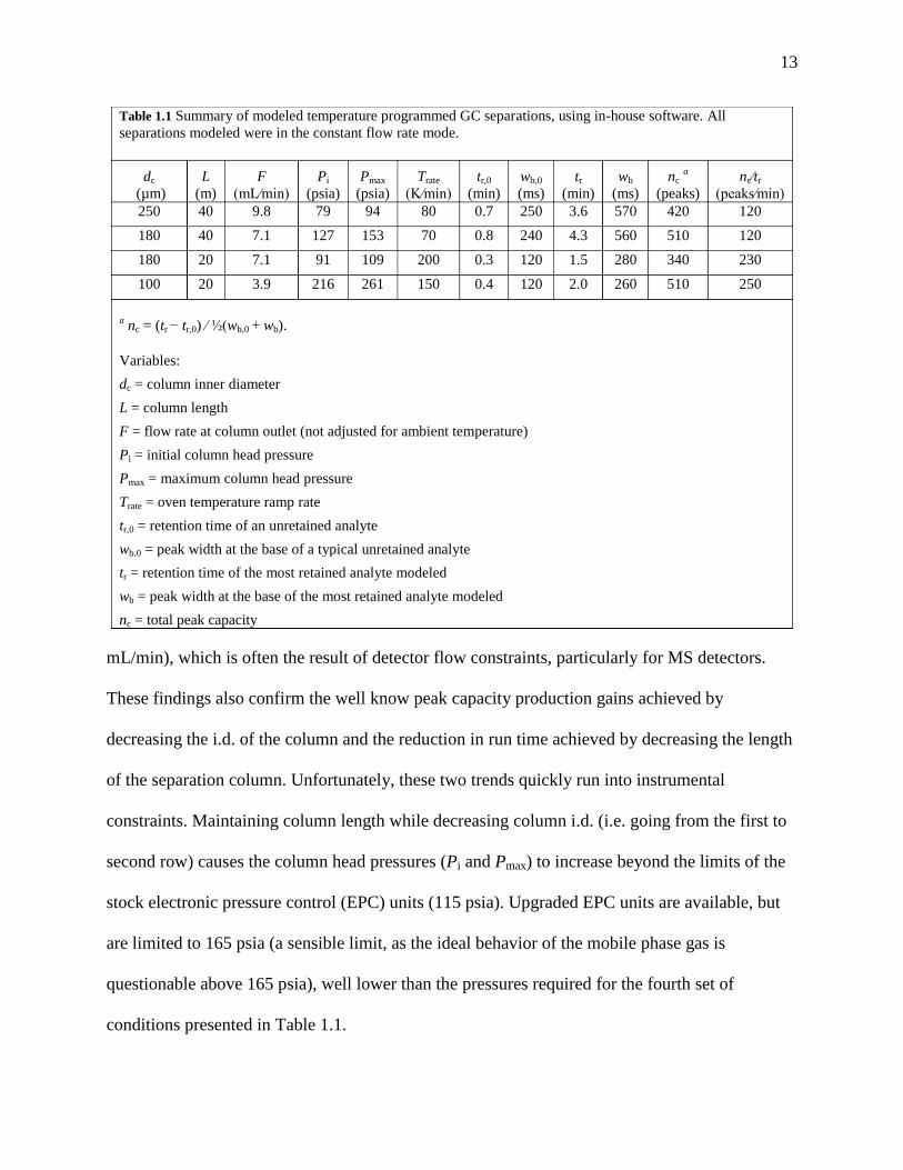
13
mL/min), which is often the result of detector flow constraints, particularly for MS detectors.
These findings also confirm the well know peak capacity production gains achieved by
decreasing the i.d. of the column and the reduction in run time achieved by decreasing the length
of the separation column. Unfortunately, these two trends quickly run into instrumental
constraints. Maintaining column length while decreasing column i.d. (i.e. going from the first to
second row) causes the column head pressures (Pi and Pmax) to increase beyond the limits of the
stock electronic pressure control (EPC) units (115 psia). Upgraded EPC units are available, but
are limited to 165 psia (a sensible limit, as the ideal behavior of the mobile phase gas is
questionable above 165 psia), well lower than the pressures required for the fourth set of
conditions presented in Table 1.1.
Table 1.1 Summary of modeled temperature programmed GC separations, using in-house software. All
separations modeled were in the constant flow rate mode.
dc
(µm)
L
(m)
F
(mL∕min)
Pi
(psia)
Pmax
(psia)
Trate
(K∕min)
tr,0
(min)
wb,0
(ms)
tr
(min)
wb
(ms)
nc a
(peaks)
nc∕tr
(peaks∕min)
250 40 9.8 79 94 80 0.7 250 3.6 570 420 120
180 40 7.1 127 153 70 0.8 240 4.3 560 510 120
180 20 7.1 91 109 200 0.3 120 1.5 280 340 230
100 20 3.9 216 261 150 0.4 120 2.0 260 510 250
a nc = (tr − tr,0) ∕ ½(wb,0 + wb).
Variables:
dc = column inner diameter
L = column length
F = flow rate at column outlet (not adjusted for ambient temperature)
Pi = initial column head pressure
Pmax = maximum column head pressure
Trate = oven temperature ramp rate
tr,0 = retention time of an unretained analyte
wb,0 = peak width at the base of a typical unretained analyte
tr = retention time of the most retained analyte modeled
wb = peak width at the base of the most retained analyte modeled
nc = total peak capacity
Table 1.1

14
The optimized linear temperature program rates in Table 1.1 are also much higher than
those available with a stock GC oven. For example, the standard Agilent 6890 is limited to a
maximum program rate of 40 °C/min over typical temperature ranges (e.g. 50 ˚C to 250 ˚C), with
deviations from linear program rates often occuring at temperatures above 175 °C and with faster
program rates [24]. Commercial instruments are now available with conductive heating systems,
allowing programming rates in excess of 10 °C/s (600 °C/min) with rapid cool down rates for
reducing total cycle time[34–36]. State-of-the-art temperature programming can be performed
with direct resistive heating of metal columns with reported rates in excess of 200 °C/s [37,38].
Despite these advances, the vast majority of GC instruments in laboratories today apply
temperature programming via a traditional convection oven, limiting standard GC methods to
temperature program rates of 30 °C/min or less.
Ultimately, the modeling must be used as a guide to parameter selection, with the
constraints of the instrumentation and the demands of the analysis driving a level of compromise.
Sections 2.3.2 and 5.2.1 also consider this process of seeking compromise between instrument
constraints and optimized conditions for the high peak capacity separations given in Table 1.1,
specifically for the 40 m x 180 µm i.d. column and the 20 m x 100 µm i.d. column.
1.4.3 Minimize off-column band broadening
As stated above, one of the conclusions to be drawn from modeling and prediction efforts
is the prevalence of off-column sources of broadening in experimental peak widths[22,39].
Common sources of off-column band broadening can include injection, non-uniform column
temperatures and dead volumes at column connections and/or within the detector. While careful
implementation of GC components can minimize many of the sources of broadening (especially

15
dead volumes), the following sections focus on improvements to the injection and detection
components of a GC instrument.
a) Injection
The standard 1D-GC auto-injector on various commercial instruments produce detected
peak widths typically greater than ~ 1 s. Researchers have devoted a significant amount of
attention to reducing the multitude of off-column sources of broadening that cause these peak
widths, particularly the broadening due to injection. The reports in this area cover a wide variety
of techniques for producing fast separations with narrow injection pulses (fluid logic gates, split
injection with high split ratios, microloop systems and micro gas valve inlets, etc.[40–44]). The
focus in the following chapters falls onto two groups of injection techniques: high speed
mechanical diaphragm valves and thermal based focusing devices.
The mechanical diaphragm valve is a commercially available device routinely used for
industrial applications requiring automated, continuous, process analysis. The valves are driven
by pressurized gas controlled by 3-way solenoid valve and are known for their minimal
maintenance requirements and long lifetimes. Hope, et al. has shown that single high-speed
diaphragm valves are capable of injection pulse widths as small as ~ 20 ms[45]. Gross and co-
workers reported that a synchronized dual diaphragm valve injection system could produce
injection pulses as small as 0.5 ms[46]. Unfortunately these valve based injection systems suffer
from two important limitations. First, an important feature of an injection system is its ability to
reproducibly provide a representative sample to the head of the separation column. As will be
shown in Chapter 2 for a valve-based injection system, the low oven temperatures that occur at
the beginning of a temperature program can cause separation to occur in the transfer line

16
between the GC inlet and the valve (though this is not a problem when valves are used to
modulate between the primary and secondary column of a GC × GC instrument). Second, the
manner in which these mechanical diaphragm valves are implemented means that only a small
portion of the sample initially introduced to the GC via the auto-injector, then to the valve, is
transferred to the column head. While this can prevent overloading of the thin film (low sample
capacity) stationary phases that are often used in high speed separations, it does mean that the
instrument may also suffer from poor detection sensitivity.
Conversely, thermal injection systems address both of the valve’s deficiencies by
stopping the migration of compounds using cryogenic temperature to focus the sample prior to
fast thermal desorption and delivery to a separation column. The cryogenic focusing step of these
thermal modulation techniques undoes any separation occurring in the transfer line by stopping
the migration of low boiling point compounds and has the added benefit of enriching the sample
concentration, leading to an improved concentration limit of detection (LOD). Thermal injection
has been reported by several groups, with the narrowest peaks on record being 20 ms wide at 4σ.
Unlike the diaphragm valves above, none of these fast thermal injection systems are currently
commercially available. There are, however commercially available GC × GC instruments (such
as the LECO Pegasus 4D), which utilize a thermal modulator to cryogenically focus effluent
from the primary column before thermal desorption onto the secondary column. These thermal
modulators are not as robust as the diaphragm valves discussed above and require a constant
supply of cryogenic liquid and so have not found much use beyond laboratory based analysis.
b) Detection
Generation of narrow GC peaks places large demands on detector design and the data

17
acquisition rate. Minimizing the volume of the detector ensures that diffusion does not broaden
the peak during detection. Inadequate sampling can also cause broadening and thus fast
acquisition rates are required for the detection of narrow peaks. Detection of narrow peaks is
commonly performed with FID (or sometimes TCD) because of its ubiquity, simplicity and fast
data acquisition rates. To detect the narrowest peaks possible with GC (5 – 10 ms wide at the
base), these detectors require faster electronics as the stock Agilent FID is capable of collecting
at most 1 or 2 points across peaks that are this narrow. To obtain the commonly advised 10 - 20
or more points across a peak acquisition rates of 2000 Hz or greater are required[47].
For complex samples, the added selectivity and dimensionality of MS data is often
required. The scanning quadruple mass spectrometer that is often utilized for GC detection is
capable of only a few scans per second while maintaining sufficient sensitivity and mass
resolution[42]. Since it is an inherently non-mass-scanning technique and is thus able to collect a
complete mass spectrum in as little as 100 µs, time-of-flight mass spectrometry is recognized as
being well suited as a detector of narrow GC peaks[47,48]. In addition, the non-scanning nature
of TOFMS means it does not suffer from the skew problems associated with scanning
instruments, making post run spectral deconvolution less problematic.
1.4.4 Improving Peak Capacity Production with GC × GC
In the context of this work, GC × GC, pioneered by Phillips and co-workers in the early
90’s[49,50], represents another tactic for increasing the overall peak capacity production of a GC
instrument. For GC × GC, two separation columns with sufficiently orthogonal stationary phases
are connected in series by a suitable injection modulation interface. Effluent from the first
column is collected and injected onto the second column by the modulation interface. The ideal

18
peak capacity, nc, GC×GC, of such a GC × GC instrument is the product of the peak capacities of
each separation dimension (superscripts have been added to Eq. 1.5 to indicate column 1)
b
2
fR,
2
b
1
o
1
fR,
1
GCGC c,W
t
W
ttn
(1.19)
where 2tR is the separation run time on column 2 (wrap-around is allowed to fully utilize the
column 2 modulation period, PM), and 2Wb is the average peak width throughout the column 2
separation. For GC × GC, where 2tR is equivalent to the modulation period, PM, and thus the
modulation ratio, MR, is equal to 1Wb divided by PM, and the resulting peak capacity production
is [51]
b
2
Rb
2
b
1
M
b
2
b
1
R
2
o
1
fR,
1
GCGC c, 1
WMWW
P
WW
t
tt
n
(1.20)
If the peak widths on column 1 can be maintained going from 1D-GC to GC × GC, the expected
theoretical increase in relative peak capacity production is then simply calculated from
b
2
M
b
2
R
b
1
GC c,
GCGC c,
W
P
WM
W
n
n
(1.21)
Since GC × GC separations should be completed in the same amount of time as an equivalent
1D-GC separation, the addition of a second column should in principle provide a dramatic
improvement in peak capacity production (though it has been demonstrated that reducing MR
will increase the effective 1 b and decrease the actual improvement [52]). From Eq. 1.21 it is
clear that a longer modulation period combined with narrow peaks on column 2 produces the
largest relative increase in peak capacity production. However, this result is deceiving because it
obscures the relationship between modulation period and column 1 peak capacity production,
where a longer modulation period in a GC × GC separation may necessitate wider peaks on the

19
column 1 to obtain comprehensive data, than would otherwise be obtained in an optimized 1D-
GC separation. Indeed, this is the point made by Blumberg and co-workers, who argued in 2008
that the typical practice of slowing down the column 1 separation to allow the long column 2
separations is caused by wide modulation pulses and is the key bottleneck to realizing the peak
capacity production gains predicted by theory[53].
1.5 HYPOTHESES
Four hypotheses concerning the improvement in peak capacity production by
minimization of both on and off-column band broadening have been set forth and will be
evaluated using the metrics and band broadening theory presented within this introduction. The
hypotheses are listed below in the order in which they are presented in the following chapters.
1.5.1 Modified Diaphragm Valve Injection
When utilized as a primary injector for temperature programmed separations, high speed
diaphragm valves have problems transferring a representative sample from the inlet to the head
of the separation column. Sample transfer problems and off-column broadening due to injection
will be minimized by coupling a resistively heated transfer line to a high-speed diaphragm valve
to provide a suitable and representative injection pulse width. Additionally, a modified flame
ionization detection (FID) electrometer will provide a data collection rate of 5 kHz to minimize
off column band broadening. It is hytpothesized that the use of long, relatively narrow open
tubular capillary columns (specifically a 40 m, 180 µm i.d. ) operated at or above the optimal
average linear gas velocity and with a 40 °C/min temperature programming rate will minimize
peak widths and maximize peak capacity production for both 1D and GC × GC separations.

20
1.5.2 High Speed Cryo-Focusing Injection
Valve based injection systems can suffer from low sensitivity and problems providing a
representative sample to the head of the separation column, especially when used in temperature
programmed separations of mixtures containing compounds with a wide range of boiling points.
An in-house built high speed cryo-focusing injector will preconcentrate the sample prior to
injection on to the separation column. It is hypothesized that this preconcentration will improve
the sensitivity and provide a representative sample for separation, while simultaneously
minimizing off-column band broadening due to injection.
1.5.3 VOC analysis via thermal injection and isothermal GC-TOFMS
High speed cryo-focusing injection is not sufficiently reproducible in practice and
difficult to implement. Commercially available thermal modulators have been shown to be
capable thermal injection systems. It is hypothesized that utilizing thermal injection via a
commercially available device will minimize off-column band broadening due to injection and
provide preconcentration of a standard VOC mixture. Selection of column parameters to
minimize off-column broadening will maximize peak capacity production while having the
added benefit of minimizing dilution of compounds during separation. Detection with the fast
data collection rate of a TOFMS will provide extra selectivity to compensate for the minimal
peak capacity provided by the isothermal separation.
1.5.4 Analysis of complex samples via optimized temperature programed GC – TOFMS
It is hypothesized that utilizing thermal injection to minimize off-column band
broadening and modeling software developed in-house to direct selection of column dimensions

21
and instrument conditions will minimize peak widths. The peak capacity production will be
sufficient to analyze very complex samples in a fraction of the time needed with traditional
separation conditions.
1.6 LIST OF WORKS CITED
[1] P. Atkins, L. Jones, C. Trapp, Chemistry: Molecules, Matter, and Change, 3rd Editions,
2nd Printing, Freeman, 1998.
[2] J.C. Giddings, Unified Separation Science, Wiley, New York, 1991.
[3] P. Donato, P. Quinto Tranchida, P. Dugo, G. Dugo, L. Mondello, J. Sep. Sci. 30 (2007)
508–526.
[4] N.E. Watson, M.M. VanWingerden, K.M. Pierce, B.W. Wright, R.E. Synovec, J
Chromatogr A 1129 (2006) 111–118.
[5] S. Thepanondh, J. Varoonphan, P. Sarutichart, T. Makkasap, Water Air Soil Poll. 214
(2011) 83–92.
[6] T. Berger, Chromatographia 42 (1996) 63–71.
[7] A.J.P. Martin, R.L.M. Synge, Biochem. J. 35 (1941) 1358–1368.
[8] A.T. James, A.J.P. Martin, Biochem. J. 50 (1952) 679–690.
[9] A.T. James, A.J.P. Martin, G.H. Smith, Biochem. J. 52 (1952) 238–242.
[10] A.T. James, Biochem. J. 52 (1952) 242–247.
[11] D.H. Desty, A. Goldup, B.H.F. Whyman, J. Inst. Petrol 45 (1959) 287–298.
[12] D. H. Desty, in:, J.C. Giddings, R.A. Keller (Eds.), Advances in Chromatography, Marcel
Dekker, Inc., New York, 1965, p. 199.
[13] R.S. Gohlke, Anal. Chem. 31 (1959) 535–541.
[14] W.C. Wiley, Science 124 (1956) 817–820.
[15] R.S. Gohlke, F.W. McLafferty, J. Am. Soc. Mass. Spectr. 4 (1993) 367–371.
[16] A.E. Thompson, J Chromatogr A 2 (1959) 148–154.
[17] I.G. McWilliam, R.A. Dewar, Nature 181 (1958) 760–760.
[18] H.A. Daynes, G.A. Shakespear, Proc. R. Soc. Lond. A 97 (1920) 273–286.
[19] G.A. Shakespear, Proc. Phys. Soc 33 (1921) 163–164.
[20] A.B. Littlewood, Gas chromatography: principles, techniques, and applications, Academic
Press, New York, 1970.
[21] H.A. Daynes, Gas Analysis by Measurement of Thermal Conductivity, The University
Press, 1933.
[22] V.R. Reid, R.E. Synovec, Talanta 76 (2008) 703–717.
[23] M.L. Lee, F.J. Yang, K.D. Bartle, Open Tubular Column Gas Chromatography : Theory
and Practice, Wiley, New York, 1984.
[24] C. Leonard, A. Grall, R. Sacks, Anal. Chem. 71 (1999) 2123–2129.
[25] K. Grob Jr., K. Grob, J Chromatogr A 207 (1981) 291–297.
[26] J.C. Giddings, Anal. Chem. 39 (1967) 1027–1028.
[27] J.C. Giddings, J Chromatogr A 703 (1995) 3–15.

22
[28] J.M. Davis, J.C. Giddings, Anal. Chem. 55 (1983) 418–424.
[29] S. Dal Nogare, W.E. Langlois, Anal. Chem. 32 (1960) 767–770.
[30] W. Harris, Programmed Temperature Gas Chromatography, J. Wiley, New York, 1966.
[31] G. Castello, P. Moretti, S. Vezzani, J Chromatogr A 1216 (2009) 1607–1623.
[32] H. Snijders, H.G. Janssen, C. Cramers, J Chromatogr A 718 (1995) 339–355.
[33] H. Snijders, H.G. Janssen, C. Cramers, J Chromatogr A 756 (1996) 175–183.
[34] K.M. Sloan, Robert V. Mustacich, Brian A. Eckenrode, Field Anal. Chem. Tech. 5 (2001)
288–301.
[35] J. Luong, R. Gras, R. Mustacich, H. Cortes, J. Chromatogr. Sci. 44 (2006) 253–261.
[36] O. . aefliger, . Jeckelmann, L. Ouali, G. Le n, nal. Chem. 2 (2010) 29–737.
[37] V.R. Reid, A.D. McBrady, R.E. Synovec, J Chromatogr A 1148 (2007) 236–243.
[38] F. Xu, W. Guan, G. Yao, Y. Guan, J Chromatogr A 1186 (2008) 183–188.
[39] F. Aldaeus, Y. Thewalim, A. Colmsjö, J Chromatogr A 1216 (2009) 134–139.
[40] G. Gaspar, P. Arpino, G. Guiochon, J. Chromatogr. Sci. 15 (1977) 256–261.
[41] R.L. Wade, S.P. Cram, Anal. Chem. 44 (1972) 131–139.
[42] H. Wollnik, R. Becker, H. Götz, A. Kraft, H. Jung, C.-C. Chen, P.G. Van Ysacker, H.-G.
Janssen, H.M.J. Snijders, P.A. Leclercq, C.A. Cramers, Int. J. Mass Spectrom. 130 (1994)
L7–L11.
[43] A.J. Borgerding, C.W. Wilkerson, Anal. Chem. 68 (1996) 701–707.
[44] M. Nowak, A. Gorsuch, H. Smith, R. Sacks, Anal. Chem. 70 (1998) 2481–2486.
[45] J.L. Hope, K.J. Johnson, M.A. Cavelti, B.J. Prazen, J.W. Grate, R.E. Synovec, Anal. Chim.
Acta 490 (2003) 223–230.
[46] G.M. Gross, B.J. Prazen, J.W. Grate, R.E. Synovec, Anal. Chem. 76 (2004) 3517–3524.
[47] M.M. van Deursen, J. Beens, H.-G. Janssen, P.A. Leclercq, C.A. Cramers, J Chromatogr A
878 (2000) 205–213.
[48] C. Leonard, R. Sacks, Anal. Chem. 71 (1999) 5177–5184.
[49] Z. Liu, J.B. Phillips, J. Chromatogr. Sci. 29 (1991) 227–231.
[50] Z. Liu, S.R. Sirimanne, D.G. Patterson, L.L. Needham, J.B. Phillips, Anal. Chem. 66
(1994) 3086–3092.
[51] W.C. Siegler, J.A. Crank, D.W. Armstrong, R.E. Synovec, J Chromatogr A 1217 (2010)
3144–3149.
[52] J.M. Davis, D.R. Stoll, P.W. Carr, Anal. Chem. 80 (2008) 461–473.
[53] L.M. Blumberg, F. David, M.S. Klee, P. Sandra, J Chromatogr A 1188 (2008) 2–16.

23
CHAPTER 2 Achieving High Peak Capacity Production for Gas
Chromatography and Comprehensive Two-Dimensional Gas
Chromatography by Minimizing Off-Column Peak Broadening*
2.1 INTRODUCTION
One-dimensional gas chromatography (1D-GC) has been an important method of analysis
for complex mixtures of volatile and semi-volatile organic compounds for several decades. Much
of the current research effort focuses on refining the general practice of 1D-GC to decrease the
analysis time, and/or to produce instrumental and computational advances that allow the analysis
of increasingly complex samples. Underlying all of these research efforts is the development of
strategies to increase the peak capacity production. [1] (Eq. 1.6). As discussed in Section 1.4, the
pursuit of high peak capacity production involves decreasing the width of chromatographic
peaks, which can be achieved by addressing off-column broadening due to injection and
detection, and on-column broadening via
application of GC theory to determine optimal pressure
and flow conditions for a given column.
In this chapter, the theoretical framework for on-column band broadening described in
Section 1.4.2 and previously reported [2] was applied to temperature programmed 1D-GC.
Utilizing this theory, a 40 m long column with a 180 µm i.d. was selected for use with a
relatively fast temperature program available from an Agilent 6890 GC. The modified injection
system (following the auto-injector), composed of a heated transfer line leading to a single
* Large portions of this Chapter have been reproduced with permission from R.B. Wilson, W.C. Siegler, J.C.
Hoggard, B.D. Fitz, J.S. Nadeau, R.E. Synovec, J. Chromatogr., A 1218 (2011) 3130–3139.

24
Table 2.1 Compounds included in the complex GC x GC
test mixture. Listed in elution order with boiling point.
Elution
Order Compound
Boiling
Point
(˚C)
1 1-propanol 97
2 benzene 80
3 1-heptene 94
4 2-pentanol 116
5 heptane 98
6 1-heptyne 100
7 1-pentanol 137
8 toluene 111
9 octane 126
10 chloro-benzene 132
11 1-cholor-hexane 135
12 ethyl-benzene 136
13 DMMP 181
14 3-heptanone 149
15 2-heptanone 151
16 o-oxylene 144
17 nonane 151
18 bromo-benzene 156
19 1-bromo-hexane 155
20 mesitylene 165
21 3-octanone 165
22 tert-butylbenzene 170
23 decane 174
24 1-br-heptane 108
25 butylbenzene 182
26 1-undecene 193
27 undecane 196
28 methyl caprylate 240
29 1,3,5-trichlorobenzene 209
30 1-bro-octane 202
31 naphthalene 218
32 1-dodecane 214
33 dodecane 215
34 tridecane 234
35 methyl decanoate 224
36 tetradecane 254
37 n-pentadecane 270
38 hexadecane 287
39 heptadecane 303
40 pristane 296
41 octadecane 305
42 nonadecane 330
43 dibutylphthalate 340
44 eicosane 344
diaphragm valve, was experimentally
characterized and implemented to minimize off-
column band broadening from the injection
process. Based on the theory for on-column
band broadening, instrumental parameters were
optimized to provide evenly distributed peak
widths throughout the separations achieved,
resulting in significantly increased peak capacity
production. The benefits of the modified
injection system are demonstrated on both 1D-
GC and GC × GC instruments.
2.2 EXPERIMENTAL
2.2.1 Reagents and Chemicals
All chemicals were reagent grade or
higher: methanol (J.T. Baker, Phillipsburg, NJ,
USA), anisole and octanol (Aldrich, Fairlawn,
NJ, USA), and tridecane (Alfa Aesar, Ward Hill,
MA, USA). A 4 component test mixture was
prepared from these neat solvents with
approximately equal concentration by volume of
each. The four solvents (components) were

25
chosen to span a boiling point range of 65 °C (methanol) to 234 °C (tridecane) to evaluate the
modified injection system. Polar analytes were included in the mixture to demonstrate that
modified injection is effective across compound classes. Gasoline was also used as a
demonstration of a complex sample, and was obtained from a local gas station. The compounds
in the complex mixture used in the GC × GC experiment are listed in the order of elution in
Table 2.1. Boiling points for each analyte were found in the CRC handbook of Chemistry and
Physics [3]. The mixture was prepared by mixing neat analytes with sufficient concentration of
each to be able to see each analyte signal.
2.2.2 Instrumentation
All chromatograms were obtained using an Agilent 6890 gas chromatograph with an
auto-injector controlled by ChemStation software (Agilent Technologies, Palo Alto, CA, USA)
modified as illustrated in Figure 2.1. The Agilent
FID was supplemented with a custom
electrometer that was built in-house and capable
of providing data acquisition at a rate of 20 kHz.
This electrometer was interfaced to a National
Instruments data acquisition board (model PCI-
MIO-16XE-50, National Instruments, Austin, TX,
USA) and the resulting data was collected using a
LabVIEW 8 (National Instruments) program
written in-house at a rate of 5 kHz. The GC
instrument was modified to use a diaphragm valve
Capillary Column
Com
merc
ial
Auto
inje
cto
r
FID
Deactivated
Steel Column
Face Mounted
Diaphragm Valve
AC
Figure 2.1 Diagram of the Agilent 6890 GC with the
modified injection system. Changes include mounting a
high-speed diaphragm valve in the GC and a high-speed
electrometer board for the FID. The valve inlet is connected
to the instrument inlet by a 15 cm resistively heated,
deactivated steel column transfer line. The transfer line is
electrically insulated from the GC by short lengths of
deactivated fused silica column.

26
(VICI, Valco Instruments Co. Inc., Houston, TX, USA), fitted with a 10 µl sample loop for
injecting a sample volume onto the column. The single valve injection system presented by Hope
and co-workers [4] was refined by face mounting the valve as described by Sinha and co-
workers [5], allowing for a wider range of oven temperatures (comfortably to 250 oC). For
samples containing higher boiling point compounds (the complex test mixture described in Table
2.1), the injection system was further refined by switching the ports flowing into the valve
(carrier gas and inlet reversed) and the outlet ports (the column and vent reversed). In this
configuration the “load” and “inject” positions are effectively switched [4]. The valve was timed
to ‘load’ for a short period after auto-injection and then ‘inject’ for the remainder of the
separation, allowing the sample loop to completely purge during the temperature program. With
this valve configuration the sample volume injected is determined by the volume of the sample
loop, not the time the valve is open. For the GC × GC experiments a second diaphragm valve,
with a 1.3 µl sample loop was added to repeatedly collect and inject the effluent from column 1
onto column 2 at a specified modulation period. Valve timing and actuation were controlled
using the same LabVIEW program described above. For the modified injection system, sample
was delivered from the GC inlet to the diaphragm valve via a 15 cm length of deactivated steel
column with a 250 µm i.d. (UADTM-5, Quadrex Corporation, Woolbridge, CT, USA). This steel
column transfer line was electrically insulated from the GC using two short lengths of
deactivated fused silica column, also with 250 µm i.d. (10079, Restek, Bellefonte, PA, USA).
The fused silica sections of the transfer line were coupled to the steel column using steel column
unions with a 250 µm i.d. bore (VICI). A variable autotransformer (Staco Energy Products,
Dayton, OH, USA) supplied ~12 V of alternating current to the transfer line via three high
temperature electrical leads placed on opposite ends of the steel column unions, hence producing

27
a heated transfer line at ~ 250 oC (measured with an infrared thermometer) leading to the
diaphragm valve with the 10 µl sample loop.
2.2.3 Chromatographic Experiments
To characterize the heated transfer line performance, 2D-like separations were completed
using the heated transfer line described above as column 1, and a 1.4 m MXT-5 Silicosteel
column (Restek) with a 180 µm i.d. and a 0.4 µm film thickness (5% phenyl/95% dimethyl
polysiloxane) as column 2. For these experiments the inlet was operated under a 5:1 split at 414
kPa absolute while the head pressure on the column 2 was also 414 kPa absolute. These
separations were performed with a modulation period of 500 ms and a 15 ms injection pulse
width. At an average volumetric flow of ~ 1 μl/ms, 15 μl are flushed through the sample loop
during injection, ensuring the 10 μl sample loop is sufficiently purged for the purpose of the
modified injection system study. The oven was held at 150 °C throughout the run.
When utilizing the transfer line for injections in both the 1D-GC and GC × GC
configurations, the inlet was operated with a split of 5:1 at a relative pressure of 207 kPa. In both
GC and GC × GC studies the oven was held at 90 °C for 0.5 min, programmed from to 250 °C at
40 °C/min, and held at 250 °C for 0.5 min. 1D-GC separations were completed using a 40 m
Rtx-5 column (Restek) with a 180 µm i.d. and a 0.4 µm film thickness (5% phenyl/95% dimethyl
polysiloxane). Valve injections were 15 ms wide unless otherwise noted in the text.
GC × GC separations were performed, using the same 40 m Rtx-5 column with a 180 µm
i.d. for column 1. For column 2 a 2 m D5 trigonal tricationic ionic liquid column with a 100 μm
i.d. and 0.0 μm film thickness was used. This novel stationary phase, developed by Payagala
and co-workers [6], consists of a tri (2-hexanamido) ethylamine core surrounded by
propylphosphonium cationic moieties. The modulating valve injected 15 ms pulses every 200

28
ms, fully evacuating the contents of the 1.3 µl sample loop. For clarity, absolute pressure at the
head of each column is specified for each separation in the text.
2.2.4 Theoretical calculations
All calculations were completed for columns of various lengths, L, and i.d., dc, holding
other parameters constant as specified. All calculations used H2 as the carrier gas and, for the
sake of brevity, using an analyte retention factor of k = 0. The diffusion coefficient of a typical
analyte in the gas phase at the outlet of the column, DG, o, was estimated for a temperature at the
beginning of the temperature program (90 °C). An analyte with a relatively low boiling point,
eluting with a k = 0 at 90 °C, such as methanol, will have a DG,o ~ 0.7 cm2/s (approximate).
Viscosity of the carrier gas, η, was calculated for each temperature based on a fit to experimental
data and is accurate for temperatures from 20 °C up to 400 °C and pressures around 101 kPa (the
pressure dependence of viscosity is sufficiently small). The outlet of the column was assumed to
be at an ambient pressure of 101 kPa.
2.3 RESULTS AND DISCUSSION
2.3.1 Evaluation of Heated Transfer Line
In order to evaluate the modified injection system for making single injections for 1D-
GC, it was initially configured in a “GC × GC mode,” with the resistively heated transfer line as
“column 1” making repeated injections onto a short, narrow column as column 2. n isothermal
separation of the four component test mixture is shown in Figure 2.2(A). Note that the four
analytes have different retention times in the transfer line (column 1) dimension, indicating that
even though the transfer line is a deactivated steel column, sufficient retention occurs if the

29
transfer line is not heated significantly above the oven temperature of 150 °C. The dotted lines in
Figure 2.2(A) demonstrate the volume sampled by a typical valve injection, defining . In Figure
2.2(A) we see the proportions of each analyte in the sample volume injected by the diaphragm
valve onto column 2 are not sufficiently constant over time, i.e., as is tuned across the column
1 time axis. If the transfer line and high-speed valve are used for a single injection, the sample
being injected onto column 2 at any given time is not consistently representative of the sample
injected on the transfer line. In contrast, with resistive heating of the transfer line to 250 °C, as
demonstrated in Figure 2.2(B), significantly reduces retention time differences in the transfer line
dimension. Unexpectedly, resistive heating of the transfer line also appears to significantly
reduce retention times on column 2, particularly for methanol, anisole, and octanol, which may
be due to conductive heating of the metal capillary being used for column 2. A single injection
from the valve at any time near the peak’s center of mass (i.e., a 15 ms pulse could in principle
M, A, O
T
Transfer Line "Column 1" Time (s)
Colu
mn 2
Tim
e (
ms)
0 1 2 3 4 5 6100
200
300
400
500
Δ
Heated
Transfer
Line
B
Transfer Line "Column 1" Time (s)
Colu
mn 2
Tim
e (
ms)
0 1 2 3 4 5 6100
200
300
400
500
M
T
O
A
Δ
Not
HeatedA
Figure 2.2 (A) 2D separation of a four analyte test mixture in a GC x GC instrumental configuration using a 15 cm
deactivated steel transfer line for the first dimension and a 1.4 m MXT-5 column as the second dimension. The
retention order is methanol (M), anisole (A), octanol (O), and tridecane (T). Both dimensions had 414 kPa of absolute
head pressure. Analytes were injected onto the second dimension column using 15 ms pulses every 0.5 s. The oven
temperature was 150 °C. The 15 ms time pulse Δ is illustrated as it depicts the pulse of sample injected using the
modified injection system in Figure 1. (B) The 2D behavior of the modified injection system is observed. The same
instrumental parameters as in (A) were used except that ~12 V were applied to the first dimension to resistively heat the
transfer line.

30
be taken between 2 s and 4 s in Figure 2.2(B)) defined by time width provided a sample with
analyte concentration proportions similar to those introduced by the auto-injector (i.e., with a
controllable split), but with much less band broadening (as will be demonstrated). In addition to
providing a narrow injection pulse, the diaphragm valve with the modified injection system also
provides a split effect, by decreasing the amount of analyte injected on the column as compared
to the amount of analyte leaving the instrument’s inlet. eak volume calculations indicate that if
the time represented by Δ in Figure 2.2(B) is a 15 ms pulse occurring 2.5 s after the initial
injection, the diaphragm valve reduces the amount of analyte transferred from column 1 to
column 2 by a factor of 160, i.e., equivalent to ~ 1:160 split. However, we shall see the 1:160
split with the modified injection system provides significantly less off-column band broadening
as compared to the original auto-injection system at either a 1:200 or 1:400 split.
2.3.2 Column and Instrument Parameter Selection
In our previous report [2] the above Theory provided analysts with broad insight into
understanding how wide “in time” peaks could in principle be in 1D-GC (assuming no off-
column band broadening). In that report, we applied the Theory to a single “typical” analyte with
a single “typical” temperature while varying column dimensions. In this report, the theory is
focused in its implementation by providing insight for column selection and instrument
parameter selection for an unretained compound (methanol, with boiling point of 64. ˚C)
eluting at the beginning of a temperature program (at 90 ˚C). We will compare and take note of
the difference between taking the Theory approach provided herein relative to the commonly
applied van Deemter plot approach.
A column with an i.d. of 180 µm was selected for this study because our previous
theoretical work [2] had shown this i.d. would likely provide a high peak capacity production

31
using a column length in the 20 m to 50 m range
(with 40 m selected), which would also allow the
maximum temperature ramp rate of 40 ˚C/min of
the oven to be utilized. The absolute head
pressure, Pi, required to obtain ūopt can be
calculated for a variety of column lengths using
Eq. 1.14. Indeed, Pi@opt (the inlet pressure at ūopt)
for a column with 180 µm i.d. is plotted as a
function of L in Figure 2.3(A). We selected L = 60
m as the longest length for the plots since this
produces a Pi@opt that is above 793 kPa, the
pressure limit of most commercial GC
instrumentation. Ideally, the column length and
flow would result in a separation occurring on the
same time scale as the oven ramp rate. For this
study a column with a 180 µm i.d. and a length of
40 m was selected because the Pi@opt of 670 kPa
(dot in Figure 2.3(A)) for the beginning of the
temperature program would allow for further
pressure programming during the temperature
program to account for the increased carrier gas
viscosity.
Calculating Pi@opt allows j, Hmin, and ūopt
0 20 40 6050
100
150
200
250
300
350
400
450
500
L (m)
ūopt(c
m/s
)
B
dc = 180 µm, T= 90 C,
DG,o = 0.7 cm2/s
: L = 40 m, ūopt = 120 cm/s
0 20 40 601
2
3
4
5
6
7
8
9
dc = 180 µm, T= 90 C,
DG,o = 0.7 cm2/s
A
L (m)
Pi@
opt (k
Pa
x 1
02)
: L = 40 m, Pi@opt = 670 kPa
0 20 40 600
50
100
150
200
250
L (m)
wb@
opt(s
)
C
dc = 180 µm, T= 90 C,
DG,o = 0.7 cm2/s
: L = 40 m, wb@opt = 160 ms
Figure 2.3 (A) Plot of inlet Pressure (Pi) at ūopt vs. column
length (L) per Eq. 1.14 for a typical analyte eluting at 90
˚C. (B) lot of the optimum average linear gas velocity ūopt
vs. column length L per Eq. 1.15 for the analyte described
above. (C) Plot of the peak width at the base, wb@opt vs. the
column length L per Eq. 1.18. The following parameters
were used to calculate the values plotted: k = 0, H2 carrier
gas.

32
to be readily determined for the same experimental parameters. The dependence of ūopt on
column length for 90 °C is shown in Figure 2.3(B) (Eq. 1.15). Subsequently, values for Wb@opt
can be calculated using Eq. 1.18. A plot of Wb@opt as a function of L is shown in Figure 2.3(C)
(Eq. 1.1 ). For the column chosen above (40 m long with a 1 0 μm i.d.), ūopt is found to be 120
cm/s (Figure 2.3(B) dot), meaning the dead time should be 33 s, while the optimal peak width is
~ 160 ms (Figure 2.3(C) dot), for the unretained peak at the beginning of the temperature
program starting at 90 °C.
This approach to band broadening theory incorporates the ūopt from the van Deemter plots
of a broad range of columns and instrument parameters into a succinct and simplified picture,
useful to the general practitioner for selecting the appropriate column dimensions for a given
application and evaluating experimental chromatographic data to determine the presence of off-
column band broadening. On the other hand, the traditional van Deemter approach applies to one
set of column dimensions, but illuminates the impact of changing linear gas velocities on the
resulting separation. For instance, the van Deemter plot, with k = 0, at 90 °C is depicted in Figure
0 100 200 300 4000
50
100
150
200
250
ū (cm/s)
H(m
m)
T= 90 C, DG,o = 0.7 cm2/s
L = 40 m, dc = 180 µm
: ūopt = 120 cm/s
Hmin = 57 µm
A
0 100 200 3000
100
200
300
400
500
600
ū (cm/s)
wb
(ms)
: ūopt = 120 cm/s
wb@opt = 160 ms
B
Figure 2.4 (A) van Deemter plot of theoretical H vs. ū for the same analyte as described in Figure 3, calculated using Eq. 1.11.
(B) Plot of theoretical wb vs. ū for the analyte described above, calculated using Eq. 1.18. The following parameters were used to
calculate the values plotted: k = 0, H2 carrier gas.
33
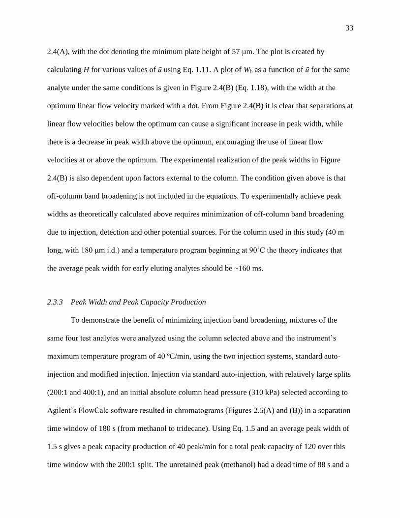
2.4(A), with the dot denoting the minimum plate height of 57 µm. The plot is created by
calculating H for various values of ū using Eq. 1.11. A plot of Wb as a function of ū for the same
analyte under the same conditions is given in Figure 2.4(B) (Eq. 1.18), with the width at the
optimum linear flow velocity marked with a dot. From Figure 2.4(B) it is clear that separations at
linear flow velocities below the optimum can cause a significant increase in peak width, while
there is a decrease in peak width above the optimum, encouraging the use of linear flow
velocities at or above the optimum. The experimental realization of the peak widths in Figure
2.4(B) is also dependent upon factors external to the column. The condition given above is that
off-column band broadening is not included in the equations. To experimentally achieve peak
widths as theoretically calculated above requires minimization of off-column band broadening
due to injection, detection and other potential sources. For the column used in this study (40 m
long, with 1 0 μm i.d.) and a temperature program beginning at 90˚C the theory indicates that
the average peak width for early eluting analytes should be ~160 ms.
2.3.3 Peak Width and Peak Capacity Production
To demonstrate the benefit of minimizing injection band broadening, mixtures of the
same four test analytes were analyzed using the column selected above and the instrument’s
maximum temperature program of 40 ºC/min, using the two injection systems, standard auto-
injection and modified injection. Injection via standard auto-injection, with relatively large splits
(200:1 and 400:1), and an initial absolute column head pressure (310 kPa) selected according to
gilent’s FlowCalc software resulted in chromatograms (Figures 2.5(A) and (B)) in a separation
time window of 180 s (from methanol to tridecane). Using Eq. 1.5 and an average peak width of
1.5 s gives a peak capacity production of 40 peak/min for a total peak capacity of 120 over this
time window with the 200:1 split. The unretained peak (methanol) had a dead time of 88 s and a

34
peak width at the base of 1.4 s, that translates into a chromatographic efficiency of N = 63,000.
Doubling the split to ratio 400:1 did not result in significantly better peak shape or width.
Using modified injection and an absolute column head pressure (586 kPa, programmed
linearly to 793 kPa) similar to that recommended by theory, a second mixture of the same four
components (albeit with different concentrations of the four components) was analyzed, resulting
in a chromatogram in a separation window of 160 s (Figure 2.6(A)). The peak width of the
unretained analyte methanol was only 250 ms and approaches the 160 ms width predicted by
theory (see Figures 2.1(C) and 2.2(B)). Unfortunately, the oven temperature program was not
synchronized with the pressure program resulting in an “isothermal-like” chromatogram in
which analyte peaks with larger retention times are progressively broadened to 750 ms for the
last peak. Also notable is the reduction in tailing of octanol using the modified injection system
as compared to the auto injector. Though the reason behind this improvement is not clear, it
appears to be another benefit of the valve-based modified injection.
80 120 160 200 240
0
1
2
3
4
5
Time (s)
FID
Resp
on
se (
V)
200:1 split, average wb= 1.5 s
86 90Time (s)
M A O T
245 250Time (s)
TM
A
80 120 160 200 240
0
0.5
1.0
1.5
2.0
2.5
3.0
3.5
4.0
Time (s)
FID
Resp
on
se (
V)
400:1 split, average wb= 1.3 s
M A O T
245 251Time (s)
T
86 90Time (s)
M
B
Figure 2.5 (A) Separation of a four analyte text mixture utilizing a 40 m x 180 µm Rtx-5 column and the standard Agilent 6890
GC auto-injection. Here, a 0.5 µl of sample was injected with a 200:1 split. (B) The same separation as Figure 2.5(A) except 0.5
µl of sample was injected with a 400:1 split. For both separations the oven was programmed from 90-250°C at the maximum
program rate of 40 °C/min. A constant volumetric flow at the column outlet of 1.3 ml/min was maintained by the instrument
software. The retention order was methanol (M), anisole (A), octanol (O), and tridecane (T).

35
To facilitate comparison with the auto-injection separations in Figure 2.5, the initial
absolute column head pressure was reduced to 310 kPa, increasing the time each test analyte
spent on the column and allowing each analyte to elute at a higher temperature and a lower
retention factor. The resulting chromatogram, with nearly constant peak widths throughout the
separation, is shown in Figure 2.6(B). The separation window was 130 s, with an average peak
width of 500 ms, resulting in a peak capacity production of 120 peaks/min (Eq. 1.5) and a total
peak capacity of 260 over this time window. The separation in Figure 2.6(B) represents a 3-fold
increase in peak capacity production with a concurrent 2.2-fold increase in total peak capacity in
20% less separation time (compared to Figure 2.5(A) or (B)). Additionally, one can objectively
compare the band broadening of the unretained methanol peak in Figure 2.6(B) to that in Figure
2.5(B), since both elute with approximately the same flow rate and temperature. The methanol
peak width of 450 ms with a retention time of 82 s corresponds to an efficiency N = 530,000, an
40 60 80 100 120 140 160 180 200
0
1
2
3
4
5
6
Time (s)
FID
Resp
on
se (
V)
Modified Injection, Void Time Optimized
43 44Time (s)
M A O T
187 190Time (s)
TM
A
80 100 120 140 160 180 200
0
0.5
1.0
1.5
2.0
2.5
3.0
Time (s)
FID
Resp
on
se (
V)
M A O T
Modified Injection, Uniform Peak Widths
M
81 83Time (s)
T
203.5 205.5Time (s)
B
Figure 2.6 (A) Separation of a four analyte test mixture utilizing a 40 m x 180 µm Rtx-5 column and the modified injection
system (resistively heated transfer line with high-speed diaphragm valve). Sample was injected onto the column using a 10 µl
sample loop and a single 15 ms valve actuation. The auxiliary electronic pressure control was used to program the absolute head
pressure on the column from 586 kPa to 793 kPa at a rate of 51.7 kPa/min during the temperature program. The same temperature
program was used as in Figure 2.5 resulting in the same retention order. (B) The same conditions as in Figure 2.6(A) except the
auxiliary electronic pressure control was used to program the absolute head pressure on the column from 310 kPa to 793 kPa at a
rate of 121 kPa/min during the temperature program, resulting in essentially the same flow rate for the unretained methanol peak
as in Figure 2.5.

36
8-fold improvement relative to the standard auto-injection with a 200:1 split. This is the most
striking evidence for the reduction of the off-column band broadening, in conjunction with the
evidence that when the column was run at optimum conditions for the unretained peak, that the
peak width experimentally observed essentially matched that expected by theory applying Eq.
1.18 with Wb ~ 160 ms predicted for these conditions per Figure 2.2(C).
2.3.4 Reproducibility Study
The four component test mixture separation was run in triplicate using the conditions in
Figure 2.6(B). These replicates were used to evaluate the reproducibility of injections made by
the heated transfer line, single high-speed diaphragm valve combination. The results are
summarized in Table 2.2. For each analyte the retention time, peak width at the base, peak height
and peak area were measured and the average reported with one standard deviation. For these
measurements of interest, the RSD% for each analyte was averaged and reported. Considering
the developmental nature of the modified injection system, values of 3.4% and 4% for the
average relative standard deviation in peak height and peak area compare favorably to the 5%
RSD% seen with traditional auto-injection (prior to applying an internal standard). The peak
widths also show good precision indicating that valve actuation time is dependable. The relative
standard deviation in analyte retention time is ~0.0006% which is very satisfactory for most
applications, although more replicates for retention time would be needed to make a more
rigorous assessment.
2.3.5 Application of Optimized Conditions to a Gasoline Sample
As a demonstration of the modified injection system under chromatographic conditions to

37
Table 2.2 Reproducibility of retention time (tR), peak width at the base, peak height and peak area, with ± one standard deviation, for
the separation of the four analyte text mixture using the modified injection system (see Figure 2.6B for representative chromatogram
and experimental conditions).
Methanol Anisole Octanol Tridecane %RSD
tR (min) 1.3684 ± 0.0001 2.2668 ± 0.0001 2.6921 ± 0.0001 3.4060 ± 0.0002 0.006 % ± 0.003
peak width@ base (ms) 459 ± 2 511 ± 5 498 ± 3 527 ± 7 0.8 ± 0.4
peak height (V) 0.65 ± 0.01 2.11 ± 0.07 0.56 ± 0.03 0.13 ± 0.01 3.4 ± 1.9
peak Area 939 ± 7 3300 ± 130 880 ± 50 209 ± 14 4 ± 3
80 100 120 140 160 180 200
0
0.5
1.0
1.5
2.0
2.5
3.0
3.5
Time (s)
FID
Resp
on
se (
V)
A
Time (s)
83 84 85 86
0
1
2
3
4
FID
Resp
on
se (
V)
Baverage wb
500 ms
156 157 158 159 160 161 162 163 164
0
0.05
0.10
0.15
0.20
0.25
0.30
0.35
0.40
Time (s)
FID
Resp
on
se (
V)
Caverage wb
500 ms
Figure 2.7 Rapid separation of a gasoline sample utilizing the 40 m x 180 µm Rtx-5 column with the modified injection
system. Sample was injected onto the column using 10 µl sample loop and a single 50 ms valve actuation. The same
temperature and pressure program was used as in Figure 2.6(B).
38
achieve optimized and constant peak widths, the instrumental parameters from the separation in
Figure 2.6(B) were applied to a gasoline sample from a local service station. Results for the
gasoline sample separation in Figure 2.7 were consistent with the previous optimized separation
in Figure 2.6(B). The separation window was ~ 120 s. Peak widths of early eluting compounds
are nearly the same width as those of late eluting compounds (~500 ms) resulting in a peak
capacity production from Eq. 1.5 of ~ 120 peaks/min.
2.3.6 Application to a GC × GC separation
To further improve the peak capacity production of the instrument, the above 1D-GC
configuration (Figures 2.6(B) and 2.7) was coupled to a 2 m column 2 via a high-speed
diaphragm valve modulator, face mounted in the GC wall to allow high temperature operation
for GC × GC [5]. Figure 2.8(A) demonstrates the potential of such a GC × GC instrument with
the separation of a complex test mixture (Table 2.1) in a 4 minute separation time window.
Figure 2.8(B) highlights a smaller region of the 2D chromatogram. Peak widths at 13% of the
peak height are ~750 ms on column 1 for both early and late eluting compounds. The lowest
contour of the chromatogram plot was chosen to be approximately 13% of the average peak
height over that region of the chromatogram, corresponding to the peak width at the base (+/- 2
standard deviations in time). On column 2 the peak widths range from 20-35 ms during the 200
ms
modulation period. Hence, Eq. 1.18 gives peak capacity production rates ranging from 500 to
800 peaks/min. With the 200 ms modulation period, and column 1 peak widths of 750 ms, the
modulation ratio was MR of 3.8, which is quite adequate for a comprehensive GC × GC
separations. Addition of the valve modulated column 2 resulted in back pressure from column 2
being applied to the primary column outlet every modulation, effecting both the dead time and

39
peak widths on column 1. These issues were minimized by delaying the actuation of the
modulator until just before the first peak eluted and increasing the initial head pressure on
column 1.
Figure 2.8(C) is the 1D separation representation resulting from summing each second
Column 1 Time (min)
Co
lum
n 2
Tim
e (
ms)
1.0 1.5 2.0 2.5 3.0 3.5 4.0 4.50
20
40
60
80
100
120
140
160
180
200
A
Column 1 Time (s)
Co
lum
n 2
Tim
e (
ms)
130 135 140 145 150 155 1600
20
40
60
80
100
120
2.15 min to 2.70 min
B
80 120 160 200 240 280
0
200
400
600
800
1000
Time (s)
Sig
nal,
Secon
d D
imen
sio
n S
um
213 216Time (s)
C
Figure 2.8 (A) GC x GC-FID chromatogram of the test mixture defined in Table 2.1 utilizing a 40 m x 180 µm Rtx-5 column for
column 1, and a 2 m x 100 μm i.d. ionic liquid column for column 2. After a 0.8 min delay post-injection to column 1, the
modulator valve onto column 2 was activated, making 15 ms injection pulses every 200 ms. The absolute head pressure on
column 1 was programmed from 517 kPa to 793 kPa during the temperature program. The absolute head pressure on column 2
was held constant at 621 kPa. (B) Detailed view of the peaks clustered between 126 s and 162 s. (C) 1D representation of Figure
8A, the result of summing the entire signal collected for column 2 onto the first dimension.
40
dimension separation in Figure 2.8(A). As the insert in Figure 2.8(C) shows, peaks on the
primary column are around 750 ms wide, resulting in a reduction of 1D peak capacity production
to ~ 80 peaks/min (Eq. 1.17). While the addition of the second column caused a 33% loss in peak
capacity production from column 1, the high-speed modulation period and narrow peaks on
column 2 increased the peak capacity production by a factor of ~10. Additionally, adding a polar
ionic liquid column 2 to the non-polar column 1 provides excellent selectivity for the separation.
The peaks eluting between 130 s and 160 s on column 1 that are not resolved in the 1D
representation in Figure 2.8(C) are resolved in the GC × GC separation of Figure 2.8(B). It is
interesting to note that this GC × GC configuration is designed around an initially optimized
primary column separation, and then utilizing the narrow peaks of the column 2 separation to
provide a true enhancement in peak capacity production going from 1D-GC to GC × GC. Hence,
the GC × GC design we report has not had the primary separation peaks purposely broadened in
order to allow longer modulation periods (e.g., several seconds instead of the 200 ms used
herein), as is the common practice. The instrumental approach reported herein provides a
concurrent selectivity advantage for GC × GC over 1D-GC, and a peak capacity production
advantage. The incentive to reduce off-column band broadening in GC technology is ever more
apparent. The benefits of addressing this issue are significant.
2.4 CONCLUSION
By reducing band broadening due to injection, substantially improved peak capacity
production was achieved using a commercial GC instrument platform. Increased peak capacity
production allows the analysis time to decrease if the total peak capacity is held constant to
address a particular analysis challenge, making these findings particularly useful in applications
requiring high throughput. These benefits were extended to GC × GC. The experimental findings

41
were also consistent with the band broadening theory presented herein. Future advances in
injection and detection technology are warranted to further advance these benefits and bring
these approaches into the hands of the general practitioner.
2.5 LIST OF WORKS CITED
[1] J.C. Giddings, Anal. Chem. 39 (1967) 1027–1028.
[2] V.R. Reid, R.E. Synovec, Talanta 76 (2008) 703–717.
[3] D.R. Lide, CRC Handbook of Chemistry and Physics, CRC Press, 2004.
[4] J.L. Hope, K.J. Johnson, M.A. Cavelti, B.J. Prazen, J.W. Grate, R.E. Synovec, Anal. Chim.
Acta 490 (2003) 223–230.
[5] A.E. Sinha, K.J. Johnson, B.J. Prazen, S.V. Lucas, C.G. Fraga, R.E. Synovec, Journal of
Chromatography A 983 (2003) 195–204.
[6] T. Payagala, Y. Zhang, E. Wanigasekara, K. Huang, Z.S. Breitbach, P.S. Sharma, L.M.
Sidisky, D.W. Armstrong, Anal. Chem. 81 (2009) 160–173.

42
CHAPTER 3 High-Speed Cryo-Focusing Injection for Gas
Chromatography: Reduction of Injection Band Broadening with
Concentration Enrichment*
3.1 INTRODUCTION
Gas Chromatography (GC) is often used in repetitive, routine, time sensitive applications
to analyze complex mixtures of volatile and semi-volatile analytes. For such applications, the
reduction of analysis time is desired, from a traditional time scale of 10 to 60 minutes down to
emerging applications in the minutes to seconds time frame, and is commonly achieved by using
short (1 to 10 m), narrow (100 to 180 µm inner diameter) columns at high linear flow velocities
and either fast temperature program ramp rates or an isothermal oven. As covered in Section 1.4,
unless off-column sources of band broadening (due to injection, detection, electronics, etc.) are
minimized, the peak widths obtained are not minimized, and the resulting chromatograms may
lack the peak capacity and separation power of GC performed on a longer, more traditional time
scale.
Chapter 3 builds upon the previous reports on thermal injection techniques described in
Section 1.4.3a by applying resistive heating to a short section of cryogenically cooled,
commercially available metal MXT column. It is shown that this simple and efficient injection
system, referred to as high-speed cyro-focusing injection (HSCFI), will produce peak widths
approaching the single digit ms time frame, while simultaneously providing sample
* Large portions of this Chapter have been reproduced with permission from R.B. Wilson, B.D. Fitz, B.C. Mannion,
T. Lai, R.K. Olund, J.C. Hoggard, R.E. Synovec, Talanta (2012).

43
Table 3.1 Boiling point, concentration (both solution phase and headspace vapor) and mass of
analyte in 30 µl of head space for each analyte in the six component sample solution.
Analyte
Boiling
Point
(°C)
Concentration in
aqueous solution
(ng/µl)
Concentration in
head space vapor
(pg/µl)a
acetone 56 50 89
methanol 65 260 76
ethanol 78 250 86
toluene 111 1 260
chlorobenzene 131 5 930b
pentanol 137 500 250 (a) Head space concentration calculations are based on aqueous concentration at room
temperature with a 1 ml head space volume, using enry’s Law constants [12].
(b) Solution containing chlorobenzene was prepared near the solubility limit, so enry’s law
calculation is not accurate and the actual headspace concentration is probably not as high as
indicated.
concentration enrichment with minimum boiling point bias (basically, all analytes injected are
trapped, focused, and thermally injected). The peak widths resulting from HSCFI are evaluated
as a function of voltage applied to the metal MXT column and the various sources of band
broadening in the instrument. Sample enrichment is demonstrated by sampling different
headspace volumes of an aqueous test solution to determine the volume of vapor that can be
cryo-focused without break through. Using enry’s law constants, the concentration of analyte
in the vapor phase and concentration and mass LODs are both determined before demonstrating
the application of HSCFI to the temperature programmed separation of a complex sample
(gasoline).
3.2 EXPERIMENTAL
3.2.1 Reagents and Chemicals
All chemicals were reagent grade or higher: methanol, pentane (J.T. Baker, Phillipsburg,
44
NJ, USA), toluene, pentanol, octane (Aldrich, Fairlawn, NJ, USA), chlorobenzene (Alfa Aesar,
Ward Hill, MA, USA), acetone (EMD, Gibbstown, NJ, USA), and ethanol (Decon Labs, King of
Prussia, PA, USA). For the peak width study a two component test mixture was made by mixing
neat pentane and octane in a 1:3 ratio by volume. For the LOD study an aqueous solution was
prepared by mixing the analytes listed in Table 3.1 with deionized water to form a six component
test mixture. The identity and boiling point of each analyte, along with the concentration of that
analyte in solution and in the head space (calculated using enry’s law constants [1]) is given in
Table 3.1. The aqueous concentration of each analyte was chosen such that peak heights would
be somewhat similar in the final chromatogram. The head space concentrations (and the mass
injected) in Table 3.1 are related to the solubility of each analyte in water as expressed in the
enry’s law constant, resulting in more water soluble analytes requiring larger solution phase
concentrations. For preparation of the six component test mixture, an initial solution of toluene
and chlorobenzene in water was made by diluting 10 mg of toluene and 50 mg of chlorobenzene
to 100 ml in water giving 100 ng/µl of toluene and 500 ng/µl of chlorobenzene. 1 ml of this
initial solution was then mixed with 5 mg of acetone, 25 mg of ethanol, 26 mg of methanol, and
50 mg of pentanol and again diluted to 100 ml of water to make the final aqueous solution with
the concentrations given in Table 3.1. A 2.0 ml screw top vial was filled with 1.0 ml of the final
aqueous solution, leaving 1.0 ml head space to be sampled by the auto-injector syringe at room
temperature. Gasoline obtained from a local gas station was used to demonstrate the HSCFI
sampling and injection with a temperature programmed separation of a complex sample.
3.2.2 Instrumentation
All chromatograms were obtained using an Agilent 6890 gas chro matograph with an
auto-injector controlled by ChemStation software (Agilent Technologies, Palo Alto, CA, USA)

45
modified for implementation and study of the HSCFI system as illustrated in Figure 3.1(A),
using flame ionization detection (FID). The
Agilent FID electrometer was replaced with
an in-house built electrometer board that
provided a data acquisition rate of up to 20
kHz in order to avoid introducing off-column
band broadening due to the FID [2]. This
electrometer was interfaced to a National
Instruments data acquisition board (National
Instruments, Austin, TX, USA) and the
resulting data was collected using a LabVIEW
2010 (National Instruments) program written
in-house at a rate of 20 kHz for the peak width
study, 10 kHz for the LOD study and 1 kHz
for the gasoline separation. Post-run data
processing (baseline correction, Savitzky-
Golay filtering, etc.) was performed in Matlab
R2010b (The Mathworks, Inc., Natick, MA,
USA).
This Agilent 6890 gas chromatograph
and modified electrometer served as a
platform to study the performance of the
HSCFI. The injection system is comprised of
Deactivated Fused Silica Transfer Line
HSCFISeparation
column
Diaphragm valve
Co
mm
erc
ial
Au
toin
ject
or
FIDInternal Unions
Cooled N2R.T. N2
Liquid N2
Copper TubingTeflon Tubing
A
Cooled N2
HSC
FI C
ircu
it
Copper Lead
MXT-5 Column
Copper Lead
B
Figure 3.1 Instrument Schematic. (A) Diagram of the modified
Agilent 6890 GC. Modifications include installing a flow
switching diaphragm valve and the HSCFI inside the oven. A
constant flow of cooled nitrogen is delivered from the liquid
nitrogen heat exchanger to the HSCFI via copper and Teflon
tubing. (B) Diagram illustrating the orientation of the Teflon
tube, MXT column and the HSCFI circuit inside the oven. The
circuit and MXT column lie in the same plane, with the Teflon
tube perpendicular. Electrical contact between the circuit and
MXT column is maintained by clamping the MXT column
between a thin sheet of copper and a solid copper post.

46
the stock auto-injector and inlet, the diaphragm valve (Valco Instruments Co. Inc., Houston, TX,
USA), and the HSCFI working in concert. Initially the carrier gas flows from the inlet through
the diaphragm valve, then to the HSCFI, and on to the column and detector. Sample is
introduced to the injection system by a microsyringe (either via auto-injector, or manually for
volumes larger than 5 µl), flash vaporized in the inlet, and transported via deactivated fused
silica transfer capillary line (Restek, Bellefonte, PA, USA) at a low flow of carrier gas to the
HSCFI, where it is cryofocused. The diaphragm valve then actuates, causing the inlet flow to be
vented and the HSCFI to be connected to an auxiliary EPC with a higher flow of carrier gas. The
time interval between the introduction of sample at the inlet and the actuation of the diaphragm
valve is referred to as the load time. A short time after the diaphragm valve actuates, an electrical
pulse is applied to the HSCFI, causing the sample to be revaporized onto the head of the
separation column. The time interval between the introduction of the sample at the inlet and the
initiation of the electrical pulse is referred to as the cryo-focusing time. For the LOD experiments
and the temperature programmed gasoline separation, the diaphragm valve was removed and the
inlet connected directly to the HSCFI, negating the need for a load time for those separations.
Figure 3.1(B) schematically depicts the HSCFI, which consists of a short section of MXT
column, (Restek) ~ 6 cm long, passing through a perpendicular Teflon tube with a 1 mm inner
diameter (i.d.). Analytes are cryo-focused in a short section of MXT column (~ 3 cm) that is
cooled by a flow of nitrogen gas which was chilled in a liquid nitrogen heat exchanger. This flow
of cooled N2 was delivered to the HSCFI in the Teflon tube and was not interrupted during the
resistive heating.
To reinject the focused analytes, the MXT column is resistively heated by delivering a
pulse of variable voltage and duration via an in-house built circuit, DC power supply (TDK-

47
Lambda, San Diego, CA, USA) and the labVIEW program described above. Appropriate
electrical contact is achieved by clamping the MXT column between a thick copper lead and a
thin flexible sheet of copper. For the peak width and LOD studies, the short copper electrical
leads required the HSCFI circuit to be housed within the GC oven, limiting oven temperatures to
60 °C for the current proof-of-principle studies. For the gasoline separation the short copper
leads were separated from the HSCFI circuit with copper wire, allowing the circuit to be placed
outside the oven and removing the limitation on oven temperatures. Further development of
HSCFI should include additional circuitry to measure the resistance of the MXT column during
heating to facilitate determining the actual temperature and heating rate of the trap.
The i.d. of all tubing (both transfer capillary line and MXT) was matched to the i.d. of the
column. Connections between the transfer lines and the HSCFI and the separation column were
made using low dead volume unions of the appropriate inner bore (Agilent Ultimate Union for
the peak width and LOD studies and Valco internal unions for the gasoline separations). For the
peak width and LOD studies the MXT column in the HSCFI was coated with 5% phenyl / 95%
dimethyl polysiloxane stationary phase, while the HSCFI used for the gasoline separation
comprised deactivated MXT column.
3.2.3 Chromatographic Conditions
The separations used to study the peak width and LOD were performed on a 1 m Rtx-5
(5% phenyl / 95% dimethyl polysiloxane) column (Restek) with a 180 µm i.d. and 0.4 µm film
thickness with the inlet and FID set to 250 °C. The gasoline separation was performed on a 20 m
Rtx-5 (5% phenyl / 95% dimethyl polysiloxane) column (Restek) with a 100 µm i.d. and 0.4 µm
film thickness with the inlet and FID set to 250 °C. For clarity, the absolute head pressure,
injection volumes, column head pressures, oven temperature, and HSCFI conditions are given in

48
the text and figure captions for each separation.
3.3 RESULTS AND DISCUSSION
To study the peak broadening produced by the HSCFI, which includes broadening
resulting from the flow dynamics and heating of the HSCFI, in addition to broadening from the
separation column and detection, 0.2 µl of a two component test mixture (pentane and octane)
was introduced via the stock auto-injector and inlet to the transfer line at 18 psi absolute (psia)
with a 300:1 split and a 60 °C oven temperature. Following a 10 s cryo-focusing step time, the
chromatogram resulting from applying a 10 V, 50 ms electrical pulse is shown in Figure 3.2. A
cryo-focusing time of 10 s was chosen for initial runs because it was much larger than the time
Time (ms)
FID
Sig
nal
(V
)
0 20 40 60 80 100 120 140 160
0
1
2
3
4
5
6
7
w ½ = 6.3 msσ = w1/2 ∙ 0.425σ = 2.7 ms
Pentane
octane
Figure 3.2 Chromatogram of pentane (72 ms) and octane (97 ms).
Sample was transferred from the inlet to the HSCFI at an absolute
column head pressure of 18 psi and a split of 300:1. After 9 s of
transfer, the flow rate was switched by the diaphragm valve to a
column head pressure of 55 psi absolute. 1 s after the change in flow
rate, a 10 V pulse was applied to the MXT column for 50 ms. The
oven was held at 60 °C throughout.

49
required for analyte to travel from the GC instrument inlet to the HSCFI, thereby ensuring
complete focusing prior to reinjection. The absolute column head pressure was 55 psi and was
applied to the HSCFI after a 9 s load time. The resulting baseline corrected chromatogram in
Figure 3.2 shows nearly baseline resolution between the two analytes, and the nearly unretained
pentane peak is only 6.3 ms wide at half height, w1/2, thus with a standard deviation σpeak of 2.7
ms.
The dependence of the electrical power applied to the MXT column on resulting peak
widths is shown in Figure 3.3. Various voltages were applied to the HSCFI, at a constan t current
level of 1 A, while maintaining a load time of 9 s, a cryo-focusing time of 10 s and a pulse
duration of 50 ms. As expected, increasing the applied voltage increases the heating rate of the
MXT column, increases the desorption rate of the analyte, and decreases the resulting peak
width. At 12.5 V (chromatogram omitted for brevity), other large peaks appeared in the
4
6
8
10
12
14
16
18
20
0 5 10 15
Pe
ak W
idth
, fw
hm
(ms)
Pulse Voltage (V)
Figure 3.3 Plot of peak width at half height as a function of
HSCFI pulse voltage for pentane. All instrument parameters
remained the same as in Figure 3.2 except for the applied
voltage. The error bars indicate +/- one standard deviation, and
the error bars at 10 V are smaller than the symbol.

50
chromatogram potentially indicating degradation of either the MXT-5 stationary phase or analyte
is occurring during HSCFI injection. No adverse effects were observed at or below 10.0 V.
Considering the minor reduction in peak width between 7.5 V and 10 V, and the poor
performance indicated in the chromatogram at 12.5 V (not shown for brevity), 10 V was selected
as the operating voltage for the HSCFI.
Based on the novel design of the HSCFI circuit, the voltage rise time should be on the
order of microseconds, meaning that very little band broadening would be introduced from the
injection electronics. The band broadening from HSCFI injection is the result of the volume
occupied by the cryo-focused analyte and the rate at which analyte is desorbed into the carrier
gas stream. Assuming that broadening due to the FID is negligible [2,3] and that variances are
statistically independent (as is commonly done for band broadening calculations), the variance of
the peak as measured at the detector (σ2
peak) can be written as
σ2
peak = σ2
vol + σ2
vap + σ2
col (3.1)
where σ2
vol is the variance due to the analyte cryo-focused volume, σ2
vap is the variance due to the
analyte vaporization time, and σ2
col is variance due to the chromatographic separation process in
the column. For the pentane peak measured above (Figure 3.2), the standard deviation of σpeak is
2.7 ms. Using in-house modeling of on-column peak broadening [4,5] that has been extended to
high speed separations, indicates the pentane peak should have a width at the base of ~ 3.2 ms,
thus a standard deviation for σcol of ~ 0.8 ms. Due to conductive cooling around the junction
between the Teflon tube and the MXT column, the maximum cryo-focusing length of MXT
column is ~ 3 cm, resulting in a maximum internal volume of 750 nl, which at a column inlet
flow rate of ~ 20 ml/min should produce a peak at most ~ 2.3 ms wide with a standard deviation
for σvol of ~ 0.6 ms. Rearranging Eq. 3.1 and evaluating for σvap yields ~ 2.5 ms, which is

51
approximately three times larger than σcol and four times larger than σvol, meaning the vast
majority of broadening for the pentane peak in Figure 3.2 is due to the desorption rate and thus
the most direct avenue to further reducing peak widths is to increase the heating rate of the MXT
column. Due to the limited data set reported herein, further study of σvap for retained analytes is
warranted for quantitatively probing (via the relationship between σvap and the enthalpy of
vaporization for various analytes) the boiling point bias inherent in HSCFI, and also the effect of
the presence of stationary phase in the trap portion of the device on the desorption rate.
To assess the LOD using HSCFI for gas phase sampling, an aqueous mixture of six
analytes of varying concentrations (given in Table 3.1) was prepared. Figure 3.4(A) shows the
chromatogram resulting from a 1 µl headspace vapor of the sample solution, introduced via a gas
tight syringe in the auto-injector and a split-less inlet with a column head pressure of 22 psia. A
10 V, 10 ms pulse was applied to the HSCFI after 5 s of cryo-focusing time, resulting in the 5 s
Time (s)
FID
Sig
nal
(V
)
0 1 2 3 4 5
0
0.01
0.02
0.03
0.04
0.05
0.06
0.0 0.5 1.0
0.00
0.03
0.06acetone
unknown
methanol
ethanol
toluene
A
Time (s)
FID
Sig
nal
(V
)
0 1 2 3 4 5
0
1
2
3
4
0.0 0.5 1.0
0
1
2
3
4 acetone
methanolethanol
toluene
acetone impurity
B
Figure 3.4 Separation of head space injection of the vapor collected above a six component aqueous mixture (see Table 3.1) via
HSCFI and a 1 m x 180 µm i.d. Rtx-5 column. Elution order: acetone, methanol, ethanol, toluene, chlorobenzene, pentanol. An
absolute head pressure of 22 psi and an oven temperature of 40 °C were maintained throughout the run. A 10 V, 10 ms pulse was
applied to the HSCFI after 5 s of cryo-focusing time. (A) 1 µl of head space vapor injected. (B) Separation in which 30 µl of head
space vapor was injected.

52
chromatogram for a total analysis time of ~ 10 s. The oven was held at 40 °C throughout the
separation. Baseline correction and a Savitzky-Golay filter (250 points, where each point is 0.05
ms) were both applied post separation run. The inset in Figure 3.4(A) focuses on the first second
of the separation and shows the elution order for the first 4 analytes. The inset also highlights the
presence of an unknown contaminant peak overlapping with methanol, making peak width and
area measurements inaccurate for methanol. The identity and source of this peak is unknown
though it is reliably visible in small volume injections and did not increase in intensity with an
increase in the vapor injection volume.
To explore the performance of HSCFI while preconcentrating a larger volume of sample
(headspace vapor) during the focusing step, injections of increasing volume (ranging from 1 µl to
40 µl) were made under conditions identical to those given above for Figure 3.4(A). Figure
3.4(B) shows the chromatogram resulting from injection of 30 µl of head space vapor collected
with the syringe from above the aqueous
solution. The chromatogram demonstrates that
as expected, increasing the volume of head
space injected increases the peak height. The
relationship between volume injected and
peak height for acetone and pentanol (the
other analytes were omitted for clarity) is
quantified in Figure 3.5. The slope, y-
intercept, and coefficient of determination for
each analyte are listed in Table 3.2 and
demonstrate that the preconcentration process
0
1
2
3
4
0 10 20 30 40
Peak
Hei
ght
(V)
Volume Injected (µL)
Acetone
Pentanol
Figure 3.5 Plot of peak height as a function of the volume of
aqueous solution head space vapor being introduced to the inlet.
For clarity, only two analytes (acetone and pentanol) were
included. Separation and HSCFI conditions are identical to those
in Figure 3.4.

53
is relatively linear, with coefficient of
determination ranging from 0.89 to 0.99. Based
on baseline noise (between 3 and 3.2 s) in the
chromatogram of Fig 4B, the peak height of each
analyte, and the concentration of analyte injected
(from Table 3.1), the concentration LODs were
calculated and reported in Table 3.3. LODs
ranging from 0.039 pg/µl to 2.2 pg/µl were achieved in the high speed separation, corresponding
to mass LODs (calculated using 30 µl as the volume injected) that ranged from 1.2 to 67 pg, and
sensitivities from 0.000 3 V∙µl/pg to 0.04 V∙µl/pg. This improved detection sensitivity is
highlighted in the inset of Fig 3.4B with the first peak in the chromatogram, which is an
unknown impurity introduced with the acetone and is not seen with the smaller injection volume
in Figure 3.4(A). The high LOD and consequent low sensitivity of chlorobenzene is due to the
initial aqueous solution being prepared near its solubility limit in water, reducing the amount of
analyte in both the aqueous solution and in the head space. Under the present trapping
conditions, 30 µl was found to be the maximum vapor volume dependably analyzed. Break
Table 3.2 For each of the six analytes in the aqueous
mixture slope, y-intercept and coefficient of determination
(R2) were calculated for the volume injected versus peak
height curves (see Figure 3.5 for representative data curves
and Figure 3.4 caption for experimental conditions).
Analyte Slope
(V/µl)
y-intercept
(V) R
2
acetone 0.15 -0.15 0.99
methanol 0.049 -0.094 0.98
ethanol 0.053 -0.11 0.99
toluene 0.067 0.020 0.89
chlorobenzene 0.025 -0.016 0.97
pentanol 0.046 -0.091 0.98
Table 3.3 For each of the six analytes in the aqueous mixture, the peak height, sensitivity, concentration LOD and mass LOD
resulting from a 30 µl injection of head space vapor and preconcentration via HSCFI (see Figure 3.4B for chromatogram and
experimental conditions) are reported. Minimum distinguishable signal used to calculate the concentration LOD is 3 times the
standard deviation of the signal collected between 3.0 and 3.2 s, and has a value of 1.8 x 10 -3 V.
Analyte
Peak
Height at
30 µl (V)
Sensitivity
(V∙µl/pg)
Concentration
LOD (pg/µl)
Mass
LOD
(pg)
acetone 4.2 0.047 0.039 1.2
methanol 1.4 0.018 0.10 3.1
ethanol 1.5 0.017 0.11 3.2
toluene 1.8 0.0068 0.27 8.1
chlorobenzene 0.77 0.00083 2.2 67
pentanol 1.3 0.0053 0.35 10

54
through was observed in the chromatogram of the 40 µl head space vapor injection (not shown
for brevity), indicated by a broad peak of unresolved compounds. Further research is necessary
to determine whether the observed break through is the result of the limited capacity of the trap,
or the limited efficiency of the trapping process at the flow rate and loading time given above.
To demonstrate the potential for application to complex samples, HSCFI was applied to
the fast separation of a gasoline sample. A relatively long (20 m), narrow (100 µm i.d.) column
was selected to minimize volumetric flow, while producing a separation time that would allow
the stock GC oven to apply an effective temperature program to the separation column. To this
end, the oven was held at 50 °C for 1 min, then ramped to 150 °C at 50 °C/min (the maximum
rate over this temperature range), and held at 150 °C for 3 min, resulting in a 6 minute
temperature program. The inlet was programmed to hold at 20 psia for 0.1 min, then ramped to
75 psia at 150 psi/min where it was held for 0.53 min. This initial ramp occurred during the first
minute of the temperature program and was meant to maximize the cryo-focusing efficiency
while minimizing the resulting peak width by focusing at a low linear flow velocity but with
HSCFI injection at a high linear flow velocity. The inlet pressure was then ramped from 75 psia
to 115 psia at a rate of 20 psi/min, and then held until the end of the program in order to
approximate a volumetric flow of 1 ml/min throughout the temperature program. The HSCFI
applied a 10 V pulse for 50 ms, with 32 s of cryo-focusing time to ~40 nl of neat gasoline. The
appearance of extra peaks in the peak width study chromatograms described above provided the
impetus for using a deactivated section of MXT column in the HSCFI design in the gasoline

55
separation. The resulting chromatogram is shown in Figure 3.6(A), with a separation time of ~
200 s. The early eluting peaks, as shown in Figure 3.6(B) are 400 ms wide at the base (four
standard deviation peak width at base definition), while the late eluting peaks (shown in Figure
40 60 80 100 120 140 160 1800
1
2
3
4
5
6
7
Time (s)
FID
Sig
nal
(V
)A
53 54 55 56 57 58 59
0
0.1
0.2
0.3
0.4
0.5
0.6
Time (s)
FID
Sig
nal
(V
)
avg w1/2 = 235 mswb = 4σ = w1/2 ∙ 1.
avg wb = 400 ms
B
154 156 158 160 1620
0.2
0.4
0.6
0.8
1.0
1.2
1.4
1.6
1.8
Time (s)
FID
Sig
nal
(V
)
avg w1/2 = 280 mswb = 4σ = w1/2 ∙ 1.
avg wb = 480 ms
C
Figure 3.6 (A) Rapid separation of a gasoline sample via a Rtx-5 column (20 m long, 100 µm i.d.), utilizing HSCFI and the stock
oven for column temperature programming. A ~ 40 nl liquid injection was cryo-focused for 32 s and reinjected by applying a 50
ms, 10 V pulse to the HSCFI. The oven was held at 50 °C for 1 min, then increased at a rate of 50 °C/min to 150 °C where it was
held for 3 min. The inlet pressure was initially held at 20 psia for 0.1 min then ramped at 150 psi/min to 75 psia, where it was
held for 0.53 min. Then, the pressure was increased at 20 psi/min to 115 psia and held until the end of the temperature program.
(B) Detail depicting peak width (average four standard deviation width at base of wb = 400 ms) of early eluting compounds. (C)
Detail depicting peak widths (average wb = 480 ms) of late eluting compounds.

56
3.6(C)), are 480 ms wide at the base. Using an average peak width of 440 ms, the total peak
capacity over the separation time is 460 peaks, with a peak capacity production of 140
peaks/min. For comparison sake, traditional GC separations, performed with an auto-injector and
200:1 split generally produce peaks ~ 2 s wide, resulting in a peak capacity production of ~ 30
peaks/min. HSCFI improves peak capacity production by a factor of 4.7 when compared to
traditional GC, an improvement similar to that seen with valve based injection [6], but with
significantly improved detection sensitivity due to the preconcentrating effects detailed herein.
3.4 CONCLUSION
With the high speed cryo-focusing injection system developed herein, peaks as narrow as
6.3 ms width at half height (w1/2) have been obtained (~ 10 ms wb), while simultaneously
providing mass LODs of less than 10 pg. Peak capacity production of 140 peaks/min has been
demonstrated using HSCFI with the stock GC oven and a temperature programming rate of 50
°C/min. It is envisaged that coupling HSCFI to a separation column that is temperature
programmed via direct resistive heating [7] may result in ~ 5 s separations with equivalent peak
capacity and separation power as a 10 min separation performed under traditional GC
parameters. Thus, HSCFI represents a significant step towards developing very fast separations
that still maintain the high peak capacity and good sensitivity associated with traditional GC.
3.5 LIST OF WORKS CITED
[1] C. Yaws, Thermodynamic and Physical Property Data, Gulf Pub. Co., Houston, 1992.
[2] G.M. Gross, B.J. Prazen, J.W. Grate, R.E. Synovec, Anal. Chem. 76 (2004) 3517–3524.
[3] A. van Es, J. Janssen, C. Cramers, J. Rijks, J. High Resol. Chromatogr. 11 (1988) 852–857.

57
[4] H. Snijders, H.G. Janssen, C. Cramers, J. Chromatogr., A 718 (1995) 339–355.
[5] H. Snijders, H.G. Janssen, C. Cramers, J. Chromatogr., A 756 (1996) 175–183.
[6] R.B. Wilson, W.C. Siegler, J.C. Hoggard, B.D. Fitz, J.S. Nadeau, R.E. Synovec, J.
Chromatogr., A 1218 (2011) 3130–3139.
[7] V.R. Reid, A.D. McBrady, R.E. Synovec, J. Chromatogr., A 1148 (2007) 236–243.

58
CHAPTER 4 High Throughput Analysis of Atmospheric Volatile Organic
Compounds by Isothermal Gas Chromatography – Time-of-Flight Mass
Spectrometry*
4.1 INTRODUCTION
Gas chromatography - mass spectrometry (GC-MS) is a widely practiced chemical
analysis technique, in particular for the analysis of volatile organic compounds (VOCs) in
ambient air. Ambient VOCs are important in a variety of fields (atmospheric chemistry,
industrial hygiene, defense, etc. [1–3]). Because ambient VOCs have both anthropogenic and
natural sources, they are often implicated in causing adverse effects on both human health and
the environment. Since ambient VOCs are often present at low analyte concentration levels, their
enrichment prior to separation and detection is an important step in the chemical analysis process
with the goal of LODs in the parts-per-billion (by volume, ppbv) range [4]. Additionally, VOC
measurements are often used to understand time-dependent processes, and therefore, may require
high temporal resolution via frequent sampling, making the minimization of the total analysis
time for the analytical technique an important challenge to address, where improvement would
be welcome [5].
As a benchmark for comparison, it is useful to summarize the standard methodologies
that have been developed for determination of VOCs in air, including EPA methods TO-1, TO-
14A, TO-15, and TO-17 methods, which differ mainly in their sampling strategies. These EPA
* Large portions of this chapter were reproduced from R.B. Wilson, J.C. Hoggard, R.E. Synovec, Manuscript Being
Prepared for Submission to Talanta (2012).

59
standard VOC analysis methods call for either cryogenic or adsorbent focusing prior to
separation and suggest long (50 m) and wide bore (200 - 300 µm inner diameter (i.d.)) columns,
with relatively thick stationary phase films (1 um) operated at temperature program rates of 8
C/min and outlet flows range from 1 to 3 mL/min [4,6–8]. The result is separation times of 30 -
50 min, LODs ranging from 0.02 (ethylbenzene) to 0.19 (3-methylhexane) ppbv (with the mass
spectrometer in full scan mode), and average peak widths of ~12 s. These peak widths result in a
separation peak capacity production of ~ 5 peaks/min and total peak capacities ranging from ~
150 to 250 [2,5]. These quantitative peak capacity metrics are based upon only the separation
time and do not take into account the GC oven cool down, which can add several minutes to the
total analysis time.
GC instrumentation has evolved through the decades to address the general elution
problem (GEP), resulting in temperature programming being the default practice to improve
peak capacity production for separations of samples containing compounds with a wide range of
boiling points. However, there are reasons and applications for which temperature programming
may not be the best solution given desired analysis goals. For example, with on-line process
analysis applications of GC, isothermal GC is commonly practiced to provide a simpler, more
robust chemical analyzer than a temperature programmed GC analyzer [9]. Indeed, the use of a
temperature program requires that the oven cool down between sample injections, often adding 5
-10 minutes to the total analysis time (with conventional ovens). For situations where high
throughput analysis is desired and the samples are not extremely complex, isothermal analysis
may be more appropriate, eliminating the need for an oven cool down step and allowing the
separation to occur during the dead time of the previous injection. Indeed, in the case of ambient
VOCs, the volatile nature of the analytes constrains the boiling point range and makes this an
60
attractive strategy.To partially offset the loss in separation peak capacity for an isothermal
separation (relative to a temperature programmed separation of equal time), while maximizing
the peak capacity generated, it is necessary for the injection, detection and separation processes
to produce narrow peaks (see Section 1.4 for details).
In Chapter 4, modeling is initially used to select column dimensions and experimental
parameters given the practical constraints of the GC-TOFMS (Agilent 6890 GC – LECO
Pegasus III TOFMS instrumental platform), and a desired separation run time that would be
conducive for high throughput analysis. Unlike previous work (Chapter 5) utilizing the thermal
modulator for thermal injection [10], the column was operated isothermally and isobarically for
the separation of a standard VOC mixture (where each analyte is nominally ~ 1 ppm) on the
primary column. The contribution of the thermal modulator (from the LECO instrument) to the
peak width was then evaluated from the widths and retention times obtained. Though the band
broadening introduced by the thermal modulator was more significant than our in house built
device for thermal injection [11], the commercial availability and robustness of the thermal
modulator made it more suitable to demonstrate thermal injection in high throughput situations.
Next, the potential peak capacity for this instrumental design is modelled using the given
experimental parameters. Finally, the preconcentration performance of thermal injection was
evaluated in terms of both injected concentration LODs and preconcentration factors.
4.2 EXPERIMENTAL
4.2.1 Theoretical Considerations for Experimental Design
In-house developed GC separation modeling software is used to predict the peak band
broadening due to the separation processes on the column alone, the separation run time, and the

61
total peak capacity for a given set of column dimensions (length and column inside diameter,
i.d.) and outlet flow rates. Based on the findings in Chapter 1 and Chapter 5, a 100 µm i.d.
column with a stationary phase thickness of 0.4 µm and operated at a volumetric outlet flow rate
of ~1 mL/min was selected for this report [10]. Choosing a column length for an isothermal
separation is primarily an exercise in balancing the available column head pressure, the desired
separation run time, and the range of compounds in the sample. Based on our separation
modeling, a 7.5 m, 100 µm i.d. column, operated at ~ 1 mL/min and 80 °C, while keeping the
column head pressure at ~ 80 psia, should produce a separation time of 35s while remaining well
within the capabilities of the electronic pressure controller (EPC) of the GC which was limited to
115 psia. For these separation conditions, modeling indicated that the peak widths (assuming
only column broadening for the moment) should be ~ 65 ms at the beginning of the separation,
and ~ 500 ms at the end (i.e. at ~ 35 s). In the absence of off-column peak broadening, the
theoretical total peak capacity for the isothermal separation was determined to approach 100
peaks at unit resolution. Based on the insight provided by the modeling effort, we experimentally
studied these column conditions to demonstrate the separation of a standard VOC mixture.
4.2.2 Samples and Reagents
A standard mixture containing 61 of the 104 volatile organic compounds (VOCs) listed in
EPA method TO-15 at an average concentration of 1.0 ppm in Nitrogen (Spectra Gases,
Branchburg, NJ) was used in this study as an example of ambient and indoor air quality analysis.
The list of total compounds in the mixture and those determined in this work, along with the
nominal concentration appears in Table 4.1.
4.2.3 Instrumentation

62
All experiments were performed using a commercially available GC × GC – TOFMS
Compound
Quantitative
Mass
Channel
tR (s)
Peak
Height
(au)
Sensitivity
(au/ppm)
3σ
Noise
(au)
LOD
(ppb)
propylene 39 9.07 200 200 13 67
freon-12 85 9.09 5200 5200 21 4.1
chloromethane 52 9.17 1600 1600 17 11
freon-114 85 9.17 5200 5200 22 4.2
vinyl chloride 62 9.23 1000 1000 21 20
1,3-butadiene 39 9.27 660 660 15 22
bromomethane 94 9.39 1100 1100 19 17
chloroethane 64 9.44 670 670 14 21
ethanol 31 9.44 1900 1900 20 10
acrolein 56 9.59 400 400 20 50
acetone 43 9.63 3500 3500 17 5.0
freon-11 101 9.61 4300 4300 18 4.3
isopropyl alcohol 45 9.64 2900 2900 15 5.1
1,1-dichloroethene 96 9.83 1100 1100 19 18
carbon disulfide 76 10.05 3200 3200 19 5.9
methylene chloride 49 9.90 1600 1600 23 14
freon-113 101 9.85 2700 2700 18 6.7
trans-1,2-dichloroethene 61 10.16 2200 2200 18 8.3
1,1-dichloroethane 63 10.16 2400 2400 21 8.7
methyl tert butyl ether 73 10.18 2600 2600 21 7.9
vinyl acetate 86 10.26 230 230 15 66
methyl ethyl ketone 43 10.45 3400 3400 17 5.0
cis-1,2- dichloroethene 61 10.62 2100 2100 19 8.9
hexane 57 10.47 1100 1100 19 18
chloroform 83 10.76 2600 2600 18 7.0
ethyl acetate 43 10.60 3300 3300 17 5.3
tetrahydrofuran 42 10.95 1100 1100 20 18
1,2-dichloroethane 62 11.24 2300 2300 21 9.0
1,1,1-thrichloroethane 97 11.24 2500 2500 16 6.2
benzene 78 11.50 2300 2300 19 8.5
carbon tetrachloride 117 11.57 2100 2100 16 7.5
cyclohexane 56 11.59 940 940 19 20
1,2-dichloropropane 63 12.27 1100 1100 23 20
trichloroethylene 95 12.30 1400 1400 21 15
Bromo- dichloromethane 83 12.45 2300 2300 19 7.9
1,4-Dioxane 88 12.46 730 730 19 26
Methyl Methacrylate 69 12.38 960 960 17 18
Table 4.1 Compounds included in the VOC test mixture. Listed in elution order. Mass channel used for quantitation,
retention time, nominal concentration, peak height, sensitivity, concentration LOD are reported. Signal is given with arbitrary
units (au)

63
instrument modified for thermal injection and isothermal GC – TOFMS analysis, employing an
Agilent 6890N gas chromatograph (Agilent Technologies, Palo Alto, CA) coupled to a Pegasus
III TOFMS and utilizing liquid nitrogen cooled thermal modulator (LECO, St. Joseph, MI), as
shown in Figure 4.1. A 7.5 m x 100 µm column with a standard 0.1 µm film SPB-5 stationary
phase (poly(5% diphenyl/95% dimethyl siloxane), Supelco, St. Louis, MO) was used, though a
column with thicker film (0.4 µm) could have provided increased column loading capacity while
not appreciably broadening the peaks due to mass transfer in and out of the stationary phase.
Relative to the commonly applied 250 µm i.d. with a 0.25 µm film column a 0.4 µm film with a
100 µm i.d. results in only a 36% decrease in column capacity per unit column length. This is
particularly relevant because the column stationary phase provides loading capacity not only for
the separation step, but also for the preconcentration and injection steps. Increasing the stationary
Heptane 43 12.13 1200 1200 17 14
Methyl Isobutyl Ketone 43 13.27 2700 2700 17 6.2
Cis-1,3-Dichloropropene 75 13.33 1400 1400 17 12
Trans-1,3-Dichloropropene 75 14.12 1500 1500 16 11
1,1,2-Trichloroethane 97 14.47 1100 1100 16 16
Toluene 91 14.44 2100 2100 18 8.8
Methyl Butyl Ketone 43 15.10 2800 2800 16 5.8
Dibromo chloromethane 129 15.68 1500 1500 17 11
1,2-Dibromoethane 107 16.27 1600 1600 17 11
Tetrachloroethylene 166 16.50 900 900 18 20
Chlorobenzene 112 18.74 1700 1700 18 11
Ethylbenzene 91 19.73 2300 2300 18 8.0
p-xylene 91 20.33 3700 3700 19 5.1
m-xylene 91 20.33 3700 3700 19 5.1
Bromoform 173 21.80 1100 1100 18 17
Styrene 104 22.20 940 940 19 20
o-xylene 91 22.48 2000 2000 19 9.3
1,1,2,2-Tetrachloroethane 83 24.00 2000 2000 18 9.1
4-Ethyltoluene 105 31.00 1700 1700 19 11
1,3,5-Trimethylbenzene 105 31.80 1700 1700 19 11
1,2,4-Trimethylbenzene 105 36.30 1500 1500 19 13
1,3-Dichlorobenzene 146 38.75 1300 1300 19 15
Benzyl Chloride 91 40.20 1100 1100 19 17
1,4-Dichlorobenzene 146 40.04 1300 1300 19 15

64
phase thickness with minimal peak broadening provides a route to further improve upon the
results reported herein.The inlet and capillary transfer line were both set to 200 °C, while the
modulator block was set to 50 °C higher than the oven temperature (130 °C). The TOFMS ion
source was set to 225 °C and a mass spectrum was collected every 10 ms (mass channels 12 –
502 m/z). The oven was held at 80 °C and the column head pressure was held at ~ 80 psia
LN
2Jets
Column
Hot
Jets
Modulator
Block
Inlet
Au
to-I
nje
cto
r
Figure 4.1 Schematic of GC – TOFMS instrument with thermal injection onto a single column (modified LECO GC
× GC – TOFMS instrument upgraded with the commercially available thermal modulator). The head of the column is
inserted through the thermal modulator and then attached to the stock inlet, before being connected to the TOFMS
via a heated transfer line. The section of column between the stock inlet and the thermal modulator, essentially acts
as short capillary transfer line. The default timing of the hot and cold jets is used with a 45 s modulation period and 2
s hot pulse to produce a narrow pulse of sample on the separation column.

65
throughout the entire run time.
To use the thermal modulator for thermal injection onto the primary column of a GC –
TOFMS, the column head was inserted backwards, through the top of the modulator block (in
the second oven), down past jet 2, then past jet 1 and out the bottom of the modulator block
before being connected to the instrument inlet, such that the modulator stages are in the same
order relative to the column flow as for normal GC × GC operation. The section of column
between the stock inlet and the thermal modulator, essentially acts as short capillary transfer line
Figure 4.2 Separation of a VOC text mixture utilizing thermal injection for sample introduction to a 7.5 m SPB-5 column (100
µm i.d.) primary separation column. Both the column head pressure (79 psia) and the oven temperature (80 °C) were held
constant throughout the run. (A) Plot of analytical ion chromatogram (AIC is the sum of mass channels listed in Table 4.1) gives
an overview of the separation. Retention order is given in Table 4.1. (B) Detail window of the AIC between 9 and 12 s.
Approximately 16 peaks appear to be partially resolved. (C) 2D plot of all mass channels for the time window in (B) demonstrates
the added selectivity provided by the TOFMS and provides evidence for 29 resolved VOCs in this region of the chromatogram.
Time (s)
AIC
(x1
03)
0 5 10 15 20 25 30 35 40 45
0
5
10
15
9 10 11 12
0
5
10
15
Time (s)
AIC
(x1
03)
9 10 11 12
38
60
80
100
120
140
160
Time (s)
m/z

66
coated with stationary phase. This could potentially lead to separation of the compounds prior to
injection on the separation column and cause the injection system to be biased towards low
boiling point compounds. This is partially mitigated by introducing the sample to the instrument
at the beginning of the modulation period, giving the high boiling point compounds sufficient
time (~ 45 s) to travel from the inlet to the first cryogenic focusing liquid nitrogen jet. To further
minimize compound discrimination, this section of column could in principle be replaced with an
integrated deactivated guard column. 500 µL of the standard gaseous mixture was transferred
from the canister to the GC inlet via a regulator set to 19 psia and a gas tight syringe (Hamilton
Company, Reno, NV). Sample was introduced to the instrument inlet approximately 90 s (2
modulation periods) after the initiation of the method to both ensure freshly cooled Nitrogen
would be used to cryo focus the sample and to allow extra time for any high boiling point
compounds from the previous run to elute from the column. In principle both of these issues
could be mitigated by further development of the instrument and method. Improved modulator
control software could reduce this sampling time to a much shorter time as it only needs to be
long enough to ensure complete cooling of the thermal injector and cryo focusing of the sample.
While increased oven temperatures, or a backflush step could be implemented to clean the
column between runs. A 45 s modulation period and 2 s hot pulse were used, along with the
default jet timing, to ensure the sample was completely transferred to the separation column.
4.3 RESULTS AND DISCUSSION
In order to better visualize the entire separation, the analytical ion chromatogram (AIC)
was constructed by summing the signal from the mass channels listed Table 4.1. The resulting
separation is plotted in Figure 4.2(A) and demonstrates that a little over 40 s was required for the
67
elution of benzyl chloride (the most retained compound). Use of the AIC is preferred over the
TIC since many of the lower m/z channels in the TIC were obscured by permanent atmospheric
gases, eg., nitrogen, oxygen, argon, and carbon dioxide that accompanied each injection. It is
evident from the chromatogram in Figure 4.2(A) that the majority of compounds in this mixture,
separated at 80 C, elute early in the separation. To highlight the peak capacity and resolving
power provided by the separation conditions in this early time window, a detail of the first 3 s of
the chromatogram is presented in Figure 4.2(B). From the AIC it appears as though there are 16
compounds in this time window, with peak widths at the base (4σ) ranging from 115 ms to 150
ms. In this region of the chromatogram the benefit provided by the TOFMS selectivity is
apparent in Figure 4.2(C), where the two dimensional (2D) plot of mass channel as a function of
retention time allows visual evidence of 29 compounds, instead of what appears to be only 16 in
Figure 4.2(B). These 29 compounds were readily quantified using selected m/z, as will be
described later herein.
Excluding off-column sources of band broadening, the on-column band
broadening, H, for an analyte with a retention factor of k as derived by Golay is given by
222,
2 2
,
22 1 6 11
96(1 ) 3(1 )
fG o c
G o L
kd uD jf d ufk kH
u k D j k D
(4.1)
where k is the retention factor of the analyte, dc is the i.d. of the capillary, df is the thickness of
the stationary phase film, DG, o is the diffusion coefficient of the analyte in the gas phase at the
outlet of the column, j and f are gas compression correction factors, DL is the diffusion
coefficient of the analyte in the stationary phase, and ū is the average linear velocity of the
carrier gas. Since H is quantitatively the length variance per column length, L, of the analyte
peak on-column, the appropriate translation to the detected peak width in units of time under
isothermal conditions is given by (as previously derived),

68
L
of
og
ocoog
bD
tkd
jD
ftdkk
L
tkjfDW
3
2
96
)1161()1(24
2
,
22
2
22
,
(4.2)
where to is the dead time for the separation conditions. A linear relationship between peak width
and retention factor, k, is generally observed for isothermal open-tubular capillary GC indicative
of separation and overall peak broadening conditions that are dominated by the middle “mass
transfer in the mobile phase” term of the Golay equation (specifically the 11k2 portion of the
middle term, which makes Wb sufficiently linear with k per Eq. (2))
As a means of evaluating the contribution of thermal injection (using the thermal
modulator for injection onto the primary column) to the band broadening of each peak, the peak
width and retention time data obtained from the 7.5 m x 100 µm i.d. column were plotted as
width at the base (4σ) as a function of the retention factor (k) in Figure 4.3, with a best fit line
resulting in an R2 value of 0.15 and a slope of 0.11. As k approaches zero in Figure 4.3
(compounds that elute in this region are nearly unretained) the peak width at the base approaches
a y-intercept value of 100 ms (FWHM of ~ 60 ms). Based on in-house modeling of GC
separations [10,12,13], a nearly unretained peak (such as propylene) eluting under these
conditions should have a peak width at the base of 88 ms, which is reasonably close the observed
value of 100 ms. The discrepancy of 100 ms versus 88 ms suggests that the off-column sources
of band broadening (injection, detection, dead volumes, etc.) are increasing the width of early
eluting compounds by ~ 14% relative to the theoretical value.
To gain a better understanding of the potential benefit toward optimizing total peak
capacity offered by implementing thermal injection, an isothermal chromatogram with peaks of
equivalent areas was simulated based on the experimental data in Figs. 4.2 and 4.3, with the
simulated chromatogram presented in Figure 4.4. Retention times and peak widths were

69
iteratively calculated such that adjacent peaks were separated by unit resolution (Rs = 1)
throughout the separation, with simulated white noise added to the chromatogram. For a
separation time window of ~ 35 s (similar to that of the VOC standard chromatogram) the peak
capacity is 114, with the last peak having a k just above 3. The peak height decreased by a factor
of 5 between the first and last peak while the peak width increased by a factor of 6. The inset in
Figure 4.5 is a detail of the first 6 s of the modeled chromatogram and emphasizes that the
majority of the separation peak capacity is produced early in the separation time where it is most
useful for this mixture of VOCs. Since the separation is isothermal there is no need to wait for
the oven to cool down and the dead time may be used as separation time for applications in
which multiple samples need to be analyzed in succession.
0
0.1
0.2
0.3
0.4
0.5
0.6
0.7
0 1 2 3 4
Peak W
idth
, W
b,t
(s)
Retention Factor, k
Figure 4.3 GC peak width at the base (4σ), Wb,t, versus the retention factor, k, using all VOCs from Table 4.1

70
We now consider the performance of this instrumental platform for providing sensitive
analytical results. LODs for each in the VOC test mixture were determined using the most
sensitive (and sufficiently selective) mass channel (m/z) for each compound in the test mixture.
The injected concentration LODs were calculated by dividing the detected noise by the analyte
sensitivity for a given compound in the test mixture. For the LOD calculation 3σ oise was
defined as three times the standard deviation of the first n s of the chromatogram collected on the
specified mass channel for the particular compound, where n is the width of the analyte peak in
time. Additionally, the sensitivity was determined using the m/z providing the largest signal,
divided by the nominal injected concentration of the analyte in the VOC mixture). The results of
0 5 10 15 20 25 30 35 40 45
0.0
0.1
0.2
0.3
0.4
0.5
0.6
0.7
0.8
0.9
1.0
Time (s)
Sig
nal
9 10 11 12 13 14 15
Figure 4.4 Simulated isothermal chromatogram in which all peaks have equal area and a unit resolution. The simulation is based
on the data from Figs. 2 and 3. Inset details a smaller time window (9-15 s) and highlights the potential peak capacity available at
the beginning of an isothermal separation

71
the LOD calculations are summarized in
Table 4.1. The injected concentration
LODs range from 4 ppb (Freon-12) to 200
ppb (naphthalene) and show no
discernable relationship to retention time.
Based on the relationship between
chromatographic peak width and retention
time that governs isothermal GC
separations, as is evident in Fig 3, it might
be expected that early eluting analytes
would have lower LODs than later eluting
analytes. The absence of this relationship
can be explained partly by the differing
sensitivities of the TOFMS mass channels
and partly by the high density of compounds towards the beginning of the separation, which
required the selection of less sensitive, but more selective mass channels for some analytes (e.g.
propyl benzene, chloromethane), in contrast to the low density of analytes eluting toward the end
of the separation, allowing for selection of the most sensitive mass channel (e.g benzyl chloride
and styrene).
Previous work has shown that the LECO modulator is a highly capable technology for
thermal injection able to produce the narrow injection pulses required for fast GC, while
simultaneously focusing (i.e., preconcentrating) the sample. In principle, focusing of the
compounds, along with the narrowness of the peaks provided by a high efficiency GC separation,
Cavg
Wb,vol
500 µL
Inject
Separate
Preconcentrate
Detect
Figure 4.5 Illustration of preconcentration produced by cryogenic
focusing provided by thermal injection. Minimizing on-column
broadening reduces the dilution of compounds that occurs during
separation and leads to low LODs. See eqs. 4.3 – 4.9

72
should result in a higher signal-to-noise ratio (S/N) and a lower LOD, as compared to a
comparable separation without preconcentration. From a S/N perspective, the separation step and
the inherent broadening processes that occur, while reducing interference between analytes,
result in some unwanted dilution of the analyte. Hence, the separation step works against
preconcentration to some extent. Thus, the minimization of on-column broadening due to the GC
separation itself is essential not only for maximizing separation power but also as a means to
maximize the detected sensitivity. We studied these issues for the instrumental platform reported
herein.
Figure 4.5 is a schematic demonstrating both the preconcentration and subsequent
dilution that occurs to analytes during the entire thermal injection - GC - TOFMS analysis. To
relate the peak detected concentration , Cpeak, to the nominal injected concentration, Cinj, and the
preconcentration factor, P, we start by assuming the moles of analyte is conserved between
injection and detection
molinj = moldet (4.3)
The number of moles injected, molinj, is related to the nominal concentration, Cinj, and the
volume injected, Winj,vol, by
molinj = Cinj ∙ Winj,vol (4.4)
Since approximately 95% (assuming a Gaussian peak model for simplicity) of analyte material
resides within ± 2σ of the peak concentration, the moles of analyte detected, moldet, may be
expressed as
moldet = Wb,vol ∙ Cave (4.5)
Where Wb,vol is the volume of analyte detected (and is calculated from the measured peak width
at the base in time, Wv,t, and the volumetric flow at the column outlet, 18.3 µL/s) and Cave is the

73
average detected concentration, which is related to the peak detected concentration, Cpeak,
through the gaussian distribution function
Cpeak = 1. ∙ Cave (4.6)
Substituting Eqs. 4.4 and 4.5 into Eq. 4.3, solving for Cave and substituting into Eq. 4.6 gives the
following expression
Cpeak = (1. ∙ inj,vol
b,vol)Cinj (4.7)
Defining the preconcentration factor, P, as
=1. ∙ inj,vol
b,vol (4.8)
Gives the desired relationship between the peak detected concentration, the injected
concentration and the preconcentration factor
Cpeak = P ∙ Cinj (4.9)
The resulting preconcentration factors are summarized in Table 4.2 and range from 420 for the
narrowest analyte peak (propylene), to 78 for the broadest analyte peak (benzyl chloride). It is
important to note that these values include all analysis steps from injection to detection. In this
system, reduction in preconcentration (compared to traditional VOC trapping systems) resulting
from the relatively low sample capacity of the standard stationary phase in the modulator is
offset by the narrow (and consequently high signal) peaks generated by the fast injection and
maintained throughout the separation process by selection of optimal instrumental parameters
within the hardware’s constraints.

74
Table 4.2 Compounds included in the VOC test mixture. Listed in elution order. Width at the base in time, volume and
preconcentration factor, P.
VOC Wb,t
(s)
Wb,vol
(μl)
P
propylene 0.10 2.0 420
freon-12 0.13 2.3 370
chloromethane 0.13 2.3 370
freon-114 0.12 2.2 380
vinyl chloride 0.12 2.2 390
1,3-butadiene 0.11 2.1 400
bromomethane 0.12 2.3 370
chloroethane 0.12 2.2 380
ethanol 0.12 2.2 380
acrolein 0.12 2.2 380
acetone 0.12 2.3 370
freon-11 0.12 2.2 390
isopropyl alcohol 0.12 2.3 380
1,1-dichloroethene 0.12 2.3 380
carbon disulfide 0.13 2.4 360
methylene chloride 0.13 2.5 350
freon-113 0.12 2.2 390
trans-1,2-dichloroethene 0.13 2.3 360
1,1-dichloroethane 0.13 2.4 360
methyl tert butyl ether 0.12 2.3 370
vinyl acetate 0.13 2.2 380
methyl ethyl ketone 0.14 2.6 330
cis-1,2- dichloroethene 0.14 2.6 330
hexane 0.14 2.5 340
chloroform 0.14 2.5 340
ethyl acetate 0.13 2.4 360
tetrahydrofuran 0.14 2.6 330
1,2-dichloroethane 0.14 2.6 320
1,1,1-thrichloroethane 0.14 2.6 330
benzene 0.15 2.7 320
carbon tetrachloride 0.15 2.7 320
cyclohexane 0.15 2.7 310
1,2-dichloropropane 0.16 2.9 300
trichloroethylene 0.16 2.9 290
Bromo- dichloromethane 0.16 2.9 290
1,4-Dioxane 0.16 3.0 290
Methyl Methacrylate 0.15 2.8 300
Heptane 0.15 2.8 300

75
Methyl Isobutyl Ketone 0.17 3.2 270
Cis-1,3-Dichloropropene 0.17 3.2 270
Trans-1,3-Dichloropropene 0.19 3.4 250
1,1,2-Trichloroethane 0.19 3.5 250
Toluene 0.19 3.4 250
Methyl Butyl Ketone 0.21 3.8 230
Dibromo chloromethane 0.21 3.9 220
1,2-Dibromoethane 0.22 4.0 210
Tetrachloroethylene 0.22 4.0 210
Chlorobenzene 0.26 4.8 180
Ethylbenzene 0.28 5.1 170
p-xylene 0.31 5.6 150
m-xylene 0.31 5.6 150
Bromoform 0.31 5.7 150
Styrene 0.32 5.8 150
o-xylene 0.32 5.8 150
1,1,2,2-Tetrachloroethane 0.35 6.5 130
4-Ethyltoluene 0.48 8.8 96
1,3,5-Trimethylbenzene 0.50 9.2 93
1,2,4-Trimethylbenzene 0.58 10.4 82
1,3-Dichlorobenzene 0.59 10.9 78
Benzyl Chloride 0.62 11.5 74
1,4-Dichlorobenzene 0.61 11.0 78
There are several issues to address concerning the performance of this fast isothermal GC
– TOFMS instrument. First, the EPA TO-15 method suggests that baseline resolution (Rs = 1.5)
of benzene and carbon tetrachloride is indicative of acceptable chromatographic performance [4],
while this fast separation provides a resolution of 0.6 between the two compounds. However, the
selectivity provided by the TOFMS compensates for the slightly lower resolution and readily
allows mathematical resolution (deconvolution) of benzene and carbon tetrachloride. Second,
while the LODs achieved by the fast GC instrument are in the ppb range suggested by the EPA,
they are several orders of magnitude larger than those presented in the literature. This is
primarily due to the large difference in sample volume being preconcentrated. Where standard
methods suggest preconcentrating up to 1 L aliquots of sample and the examples in the literature
use 25 – 600 mL aliquots of sample, the LOD presented herein are calculated from

76
preconcentration of a 500 µL aliquot of sample. Future work should address this issue by
exploring thermal injection’s ability to preconcentrate larger sample volumes via an increase in
the column stationary phase thickness.
4.4 CONCLUSIONS
With the LECO thermal modulator configured to provide thermal injection, a primary
column, and careful selection of column dimensions and flow conditions according to theoretical
modeling, band broadening due to both injection and the column has been significantly reduced.
This preserved the focusing provided by thermal injection and resulted in preconcentration
factors as high as 420. Isothermal conditions combined with the mass selectivity provided by
TOFMS resulted in a relatively high total peak capacity (114 peaks), high throughput analysis
(total separation run time of 45 s) with injected concentration LODs as low as 4 ppb.
4.5 LIST OF WORKS CITED
[1] B.K. Lavine, N. Mirjankar, R. LeBouf, A. Rossner, Microchemical Journal (n.d.).
[2] A. Ribes, G. Carrera, E. Gallego, X. Roca, M.J. Berenguer, X. Guardino, Journal of
Chromatography A 1140 (2007) 44–55.
[3] M.R. Ras, R.M. Marcé, F. Borrull, Environmental Monitoring and Assessment 161 (2009)
389–402.
[4] US Environmental Protection Agency, Compendium Method TO-15, Determination of
Volatile Organic Compounds (VOCs) in Air Collected In Specially-Prepared Canisters And
Analyzed By Gas Chromatography/Mass Spectrometry (GC/MS), Cincinnati, OH, 1999.
[5] M. de Blas, M. Navazo, L. Alonso, N. Durana, J. Iza, Science of The Total Environment
409 (2011) 5459–5469.
[6] US Environmental Protection Agency, Method TO-1, Method For The Determination Of
Volatile Organic Compounds In Ambient Air Using TENAX® Adsorption And Gas
Chromatography/Mass Spectrometry (GC/MS), Cincinnati, OH, 1984.
[7] US Environmental Protection Agency, Compendium Method TO-14A, Determination of
Volatile Organic Compounds (VOCs) in Ambient Air Using Specially Prepared Canisters

77
With Subsequent Analysis By Gas Chromatography, Cincinnati, OH, 1999.
[8] US Environmental Protection Agency, Compendium Method TO-17, Determination of
Volatile Organic Compounds (VOCs) in Ambient Air Using Active Sampling Onto Sorbent
Tubes, Cincinnati, OH, 1999.
[9] J.S. Nadeau, R.B. Wilson, B.D. Fitz, J.T. Reed, R.E. Synovec, J. Chromatogr., A 1218
(2011) 3718–3724.
[10] R.B. Wilson, J.C. Hoggard, R.E. Synovec, Anal. Chem. 84 (2012) 4167–4173.
[11] R.B. Wilson, B.D. Fitz, B.C. Mannion, T. Lai, R.K. Olund, J.C. Hoggard, R.E. Synovec,
Talanta (2012), http://dx.doi.org/10.1016/j.talanta.2012.03.054.
[12] G.M. Gross, B.J. Prazen, J.W. Grate, R.E. Synovec, Anal. Chem. 76 (2004) 3517–3524.
[13] V.R. Reid, R.E. Synovec, Talanta 76 (2008) 703–717.

CHAPTER 5 Fast, High Peak Capacity Separations in Gas
Chromatography – Time-of-Flight Mass Spectrometry*
5.1 INTRODUCTION
Gas chromatography-mass spectrometry (GC – MS) is an important chemical analysis
tool for volatile and semi-volatile compounds in many types of complex samples (food, fuels,
metabolomics, etc. [1–6]). Considerable effort has been aimed at developing instrumentation to
decrease the separation time for routine analysis of simple to medium complexity samples via
improved injection techniques and implementation of narrow bore columns[7–9], as well as to
increase the information generated in the analysis of very complex samples via GC × GC
separations [10–12]. While lengthy sample preparation procedures may render high speed
separations superfluous [13], recent advances in sample preparation technology and automation
have reduced sample preparation time, leading to renewed interest in applying fast GC
separations for the analysis of even the most complex samples.
This interest in applying fast GC separations must be considered concurrent with
addressing the emerging challenges in chemical analysis by improving peak capacity production
(Eq 1.6), and/or total peak capacity (Eq 1.5). As described in Section 1.4, meeting this challenge
reduces to the need for smaller peak widths, which translates into more peaks fitting into a given
separation time window. One analytical strategy to optimize the information content of a GC –
* Large portions of this Chapter have been reproduced with permission from R.B. Wilson, J.C. Hoggard, R.E.
Synovec, Anal. Chem. 84 (2012) 4167–4173.

79
MS separation could be to hold constant the separation time, while reducing the average peak
width, resulting in an overall increase in the total peak capacity. Alternatively, another analytical
strategy could be to maintain the total peak capacity constant, by concurrently reducing the
average peak width and the separation run time. This second strategy provides for higher
throughput analyses, while maintaining the information content in a given chromatogram. In
Chapter 5 the goal is to maximize peak capacity production by optimizing commercial
instrumentation and then applying that peak capacity production such that the total peak capacity
generated is greater than or essentially identical to that typically requiring a 40 – 60 min GC –
MS separation run time. The result will be a ~ 5-fold or greater improvement in peak capacity
production, to facilitate high throughput analysis applications.
To put our research effort into context, we note that for recently reported metabolomics
studies (for example), using commercially available instrumentation with automated solid phase
micro extraction (SPME) in some cases and split or split-less injection combining 30 m x 250
µm inner diameter (i.d.) columns, peak widths ranging from 4 to 10 s were reported, resulting in
peak capacity production ranging from 6 to 15 peaks/min, and a total peak capacity of ~ 200 to
500 peaks (at unit resolution) for a separation run time typically ~ 40 to 60 min. [4–6] In this
report, we shall use these numbers as benchmarks to compare the performance of the
instrumental platform we describe.
In Chapter 5, modeling is initially used to select column dimensions and experimental
parameters given the practical constraints of the Agilent 6890 GC – LECO Pegasus III TOFMS
instrumental platform. We then evaluated the LECO thermal modulator as a means of
cryogenically focusing and re-injecting sample directly onto the primary separation column of a
GC – TOFMS, referred to herein as thermal injection. For this initial study, a short column was
80
operated isothermally and isobarically. In principle, thermal injection provides a state-of-the-art
cold trap injection. Next, the separation of neat gasoline using traditional GC injection practices
is compared to the separation using thermal injection, with peak widths modeled by our software
for comparison and guidance of the experiment. Finally, a relatively fast GC – TOFMS
separation (~ 7 min with ~ 660 ms peak widths on average) is applied to the analysis of the
metabolites in a complex sample, namely, the SPME sampled headspace of urine vapor.
5.2 EXPERIMENTAL SECTION
5.2.1 Theoretical Considerations for Experimental Design
For the Agilent 6890 GC – LECO Pegasus III TOFMS instrumental platform applied in
this report, there are three primary constraints. First, the TOFMS requires a relatively low
pressure to operate at high sensitivity and while providing experimental spectra with maximal
similarity to library spectra. In general, to obtain optimal mass spectral data, the analyst should
limit the volumetric flow rate to a maximum of ~ 2 mL/min at the column outlet. Second, over
the broad range of temperatures required for the temperature programmed separation of complex
samples (40 °C – 300 °C) the stock oven of the Agilent 6890 is capable of ramping at 30 °C/min
– 40 °C/min. The third instrumental constraint is that the column head pressure is limited to 165
psia by the Agilent high pressure GC inlet.
Given these three hardware constraints we sought to choose column dimensions and
operating conditions that would both push the instrument to the limits of the hardware and
optimize total peak capacity and peak capacity production, concurrent with minimizing
separation time, for the goal of facilitating a high throughput analysis GC – TOFMS platform.

81
Table 5.1
Table 5.1. Summary of modeled temperature programmed GC separations, using in-house software building on
our previous modeling of band broadening in GC separations, [14,15] and based on the work of Snijders et al.
[16,17] All separations modeled were in the constant flow rate mode, except the last set of conditions with a
constant pressure of 160 psia.
dc
(µm)
L
(m)
F
(mL∕min)
Pi
(psia)
Pmax
(psia)
Trate
(K∕min)
tr,0
(min)
wb,0
(ms)
tr
(min)
wb
(ms)
nc a
(peaks)
nc∕tr
(peaks∕min)
250 40 9.8 79 94 80 0.7 250 3.6 570 420 120
180 40 7.1 127 153 70 0.8 240 4.3 560 510 120
180 20 7.1 91 109 200 0.3 120 1.5 280 340 230
100 20 3.9 216 261 150 0.4 120 2.0 260 510 250
250 b 40 1.0 29 33 10 3.0 2200 24.0 4800 360 15
250 40 1.8 36 44 30 2.0 1100 11.0 1900 360 33
180 40 1.8 66 79 30 1.8 720 9.8 1300 470 48
180 20 1.8 48 55 30 0.7 380 6.5 1200 440 68
100 c 20 2.1–1.6 160 160 30 0.5 180 5.5 880 560 100
a nc = (tr − tr,0) ∕ ½(wb,0 + wb).
b Modeling of conditions typically applied.
5, 6
c Modeling of conditions used in this report at constant Pi, causing flow rate to decrease throughout the run.
Variables:
dc = column inner diameter
L = column length
F = flow rate at column outlet (not adjusted for ambient temperature)
Pi = initial column head pressure
Pmax = maximum column head pressure
Trate = oven temperature ramp rate
tr,0 = retention time of an unretained analyte
wb,0 = peak width at the base of a typical unretained analyte
tr = retention time of the most retained analyte modeled
wb = peak width at the base of the most retained analyte modeled
nc = total peak capacity
As covered in Section 1.4.2 and summarized here for clarity, modeling software written
in-house was used to predict the peak broadening due to the separation processes on the column
alone, the separation time, the total peak capacity, and the peak capacity production for given set
of column dimensions (length and i.d.), temperature programming conditions, and outlet flow
rates. The findings of the separation modeling are summarized in Table 5.1 (which also includes

82
the columns from Table 1.1 for clarity). One finding of the modeling was that even for 100 µm
columns, the optimal volumetric outlet flow rate of ~ 4 mL/min is too large for the TOFMS used
for this report (and indeed for most TOFMS instruments in use), necessitating that the column be
operated at a volumetric outlet flow rate lower than optimum. Note that the optimum
volumetric outlet flow rate is defined as the minimum in the well known H versus u (linear flow
velocity) Golay plot, and that the optimum linear outlet flow (and therefore the optimum
volumetric outlet flow rate) is independent of column length. Moreover, for 180 and 250 µm i.d.
columns, the optimum volumetric outlet flow rate is ~ 7 mL/min and ~ 10 mL/min, respectively,
making the situation worse. Therefore, use of a 100 µm i.d. column operated at a volumetric
outlet flow rate of ~2 mL/min is closer to ideal conditions, and hence is the i.d. selected for this
report, using a 0.4 µm film thickness to provide sufficient sample loading capacity while keeping
the band broadening contribution due to mass transfer in and out of the stationary phase to a
relatively low level. Choosing a column length is primarily an exercise in balancing the
available column head pressure and available temperature programming rates. Based on our
modeling, summarized in Table 5.1, for a 20 m, 100 µm i.d. column, operated between 1.6 and
2.1 mL/min, a temperature programming ramp rate of 30 °C/min could be effectively applied,
while keeping the column head pressure constant at ~ 160 psia, sufficiently within the
capabilities of the upgraded electronic pressure controller (EPC) implemented with the GC,
which was limited to 165 psia. For these separation conditions, modeling indicated that the peak
widths (assuming only on-column broadening) should be ~ 180 ms at the beginning of the
separation, and ~ 880 ms at the end, with separation time window of 5 min (total separation run
time ~ 6 min). Hence, the theoretical total peak capacity was found to be approaching 600 peaks
at unit resolution. Certainly, a temperature programming rate higher than 30 °C/min could in
83
principle be applied, and the peaks could be maintained at ~ 200 ms throughout a shorter
separation run time. We elected to use the instrument under conditions relatively consistent to
those most practitioners would face. In contrast, the modeling of separation conditions typically
applied, for example, with metabolomics studies (see Table 5.1, for the 40 m, 250 µm i.d.
column, operated at a constant 1 mL/min flow rate), the theoretical total peak capacity is ~ 360,
in a much slower separation approaching ~ 30 min, which is consistent with the experimental
reports discussed earlier4-6
. Based on the insight provided by the modeling effort, we
experimentally studied the 20 m, 100 µm i.d. column conditions (as modeled in Table 5.1) to
demonstrate the separation of two complex samples: gasoline and the headspace vapor of urine
sampled by SPME.
5.2.2 Samples and Reagents
For the initial study, the seven component mixture used to evaluate the peak widths
produced by the thermal injection (via the thermal modulator used for injection with GC –
TOFMS) was made by mixing approximately equal volumes of neat pentane, carbon
tetrachloride, 1,2-dichloroethane, octane, toluene, 1,1,2-trichloroethane, and nonane. For the
subsequent studies, the gasoline and urine samples used to demonstrate the separation of
complex samples were collected from local sources.
5.2.3 Solid Phase Micro Extraction Sample Preparation
For SPME sampling of the urine headspace vapor, a 65 µm PDMS-DVB SPME fiber
(Supelco, PA, USA) served to preconcentrate metabolites and other analytes. The fiber was
conditioned at 250 °C for 15 min prior to sample extraction. For sample preparation via
headspace SPME, a given sample was heated in a water bath to 60 °C for 15 min, after which the

84
SPME fiber was exposed to the headspace for 15 min.
5.2.4 Instrumentation
All experiments were performed using a modified GC × GC – TOFMS instrument,
employing an Agilent 6890N gas chromatograph (Agilent Technologies, Palo Alto, CA) in
conjunction with a LECO Pegasus III TOFMS upgraded with the commercially available
thermal modulator (LECO, St. Joseph, MI), as shown in Figure 5.1. To evaluate the peak widths
produced by the thermal modulator, a 4 m x 100 µm column with a standard 0.1 µm film Rtx-
200 stationary phase (trifluoropropylmethyl polysiloxane, Restek, Bellefontaine, PA) was used.
For separations of the gasoline and urine samples, a 20 m x 100 µm column with 0.4 µm film
Rtx-5 stationary phase (5% phenyl/95% dimethyl polysiloxane, Restek, Bellefontaine, PA) was
applied, with the thicker film providing sufficient column loading capacity while not appreciably
broadening the peaks due to mass transfer in and out of the stationary phase. The 0.4 µm film
with a 100 µm i.d. results in only a 36% decrease in column capacity per unit column length,
relative to the commonly applied 250 µm i.d. with a 0.25 µm film. [5,6] The inlet and capillary
transfer line were set to 250 °C and 280 °C, respectively, while the modulator block was set to
40 °C higher than the oven temperature. The TOFMS ion source was set to 225 °C and a mass
spectrum was collected every 10 ms (mass channels 12 – 502 m/z). The oven was held at 80 °C
and the column head pressure was held at 40 psia throughout the entire run time on the 4 m
column during the initial study. For the gasoline separation, the oven was held at 40 °C for 1.25
min, then ramped to 250 °C (at 30 °C/min) and held for 0.5 min. For the urine headspace/SPME
separation, the oven was held at 40 °C for 1.25 min, then ramped to 280 °C (at 30 °C/min) and
held for 0.5 min. For both the gasoline and urine separations the column head pressure was held
at 160 psia throughout the run, requiring an upgraded split/split-less inlet and EPC capable of

85
controlling the pressure from 15 psia to 165 psia (Agilent Technologies).
To use the thermal modulator for thermal injection onto the primary column of a GC –
TOFMS, the column head was inserted backwards, through the top of the modulator block (in
the second oven), down past jet 2, then past jet 1 and out the bottom of the modulator block
before being connected to the instrument inlet, such that the modulator stages are in the same
LN
2Jets
Column
Hot
Jets
Modulator
Block
Inlet
Au
to-I
nje
cto
r
Figure 5.1 Schematic of GC – TOFMS instrument with thermal injection onto a single column (modified LECO GC ×
GC – TOFMS instrument upgraded with the commercially available thermal modulator). The head of the column is
inserted through the thermal modulator and then attached to the stock inlet, before being connected to the TOFMS via a
heated transfer line. The section of column between the stock inlet and the thermal modulator, essentially acts as short
capillary transfer line. The default timing of the hot and cold jets is used with a 45 s modulation period and 2 s hot
pulse to produce a narrow pulse of sample on the separation column.

86
order relative to the column flow as for normal GC × GC operation. The default timing of the hot
and cold jets was used with a 45 s modulation period and 2 s hot pulse to ensure the sample was
completely transferred to the separation column. Sample was introduced to the instrument inlet
45 s (1 modulation period) after the initiation of the method ensuring freshly cooled Nitrogen
would be used to trap the sample. A volume of 0.2 µL of both the 7 component mixture (for the
initial band broadening study) and the gasoline sample were introduced to a split-less inlet via a
0.5 µL syringe (Hamilton, Reno, NV). The urine headspace vapor sample was introduced via the
SPME fiber described previously described and a split-less inlet set to 200 °C.
5.3 RESULTS AND DISCUSSION
5.3.1 Evaluation of Thermal Modulator for Thermal Injection in GC – TOFMS
In previous work using the thermal modulator, as designed for injection from the primary
column onto the secondary column in GC × GC separations, the narrowest peaks produced are
~50 ms wide, [18] a width that is certainly compatible with the broadening modeled above for
the 20 m x 100 µm i.d. column. In the initial study using the instrument set up as in Figure 5.1
for thermal injection, we evaluated the suitability of the thermal modulator for introducing
sample to the head of a primary separation column. A short column (4 m) with a 100 µm i.d.
was operated isothermally for the separation of a simple 7 component mixture. Figure 5.2 is the
chromatogram recorded on mass channel 43 (for clarity) for this separation and shows the nearly
unretained pentane peak has a full width at half maximum (fwhm) of 54 ms, and a four standard
deviation width at the base of 92 ms (4σ = 1. ∙ fwhm, so σpeak = 23 ms), applying a Gaussian
peak shape model. According to in-house theoretical modeling an unretained peak for these
separation conditions should be broadened by the column to a width at the base of 67 ms (σcol =

87
17 ms). Since the TOFMS likely does not contribute significantly to the peak width and the
variances are statistically independent (a common assumption for chromatographic band
broadening calculations), the variance of the detected peak σ2
peak can be written as
σ2
peak = σ2inj + σ
2col (5.1)
where σ2
inj is the band broadening variance due to injection, and σ2
col is the variance due to the
column only. Equation 1 assumes that σ2
inj is the major contributor to off-column peak
broadening, which is very likely for the experimental conditions. Here we are determining to
what extent σ2
peak measured in the experiment agrees with σ2
col predicted by theoretical modeling,
4.0 4.5 5.0 5.5 6.0 6.5
0.0
0.5
1.0
1.5
2.0
2.5
Time (s)
4.3 4.4 4.5
wb = 92 ms
TIC
(x1
04)
Figure 5.2 Separation of a 7 analyte test mixture utilizing thermal injection for sample introduction to a 4 m Rtx-200 column
(100 µm i.d.) primary separation column. Plot of mass channel 43 shows the narrow first peak to be 92 ms wide at the base. Both
the column head pressure (40 psia) and the oven temperature (80 °C) were held constant throughout the run. Retention order:
pentane, carbon tetrachloride, 1,2-dichloroethane, octane, toluene, 1,1,2-trichloroethane, and nonane.

88
in order to demonstrate to what extent σ2
inj has been minimized experimentally. Given that σcol =
17 ms and σpeak = 23 ms, σinj is estimated by Eq 5.1 to be 16 ms, a value that is far less than the
σcol expected for a 20 m, 100 µm i.d. column, strongly supporting the conclusion that the
modulator causes negligible broadening to the peak width observed in GC – TOFMS separations
with the 20 m, 100 µm i.d. column. Maximal peak capacity will be achieved for this style of
injection, given the other instrumental parameters.
5.3.2 Demonstration of GC – TOFMS with Thermal Injection to Complex Samples
For the demonstration of this instrumental technology for high peak capacity and high
throughput separations, two complex samples were analyzed: a neat gasoline and the SPME
headspace sampling of urine vapor. In Figure 5.3(A) the total ion current (TIC) of the gasoline
separation is shown, demonstrating the complexity of the sample. Figure 5.3(B) shows the first
peak in the separation eluting with a width at the base of 290 ms. At a scan rate of 100 Hz, ~ 30
spectra are collected across this narrowest peak. Figure 5.3(C) shows a later eluting peak, which
has a width at the base of 800 ms. In order to optimize the signal-to-noise ratio (S/N) of this and
all GC – TOFMS separations, spectra were averaged along the separation time axis such that all
peaks had ~ 10 spectra per peak width at the base (four standard deviation peak width). With all
peaks defined by ~ 10 points, the spectra averaging introduced only ~ 3% additional peak
broadening [19]. Averaging these two widths gives a width of 550 ms, resulting in a peak
capacity production of ~ 110 peaks/min and a total peak capacity of ~ 580 peaks during a
separation window of 5.3 minutes for the gasoline. Indeed, this total peak capacity
experimentally obtained is consistent with the theoretical modeling presented in Table 5.1
(conditions in the last row for the 20 m, 100 µm i.d. column, operated with a constant inlet
pressure of 160 psia.

89
For comparison purposes, the same gasoline sample was injected onto the same column
with the same flow and temperature conditions but using the stock injection system on the
instrument with
an auto-injector and a 100:1 split. In the interest of brevity the separation with the 100:1 split is
not shown, but the following discussion highlights the increased peak capacity generated by
thermal injection by contrasting peak widths from the same time regions for each
chromatographic separation. In the separation using standard auto-injection with a 100:1 split,
Figure 5.3 Separation of gasoline utilizing a 20 m x 100 µm Rtx-5 column with 0.4 µm film, and the thermal modulator for
thermal injection to cryo-focus and reinject the sample. The oven was held at 40 °C for 1.25 min, then ramped at 30 °C/min to
250 °C and held for 0.5 min, while the column head pressure was held at 160 psia throughout the separation. (A) The total ion
current (TIC) of the entire separation run time. (B) TIC of the first peak in the separation, measuring 290 ms width at the base
(4σ). (C) representative later eluting peak (TIC), measuring 800 ms width at the base. (D) Overlay plot of the TIC and
selective mass channels for 6 late eluting peaks demonstrates the benefit of the added selectivity provided by the TOFMS.
Time (min)
TIC
(x1
06)
A Gasoline
0 1 2 3 4 5 6 7
0
1
2
wb = 800 ms
Time (min)
TIC
(x1
05)
3.97 3.98 3.99 4.000
1
2
3
4
5C
4.07 4.10 4.13
0.0
0.4
0.8
1.2
1.6
2.0m/z = 85m/z = 84m/z = 71m/z = 83TIC
Time (min)
Scale
d S
ign
al
D
wb = 290 ms
Time (min)
TIC
(x1
04)
0.616 0.620 0.624 0.628
0
1
2
3
4 B

90
the peaks around the time window of Figure 5.3(B) averaged 1.2 s wide at the base, while the
peaks around the time window of Figure 5.3(C) also averaged 1.2 s wide at the base. This gives a
peak capacity production of ~ 50 peaks/min and a total peak capacity of ~ 270 peaks during the
same 5.3 min separation time window. Therefore, thermal injection via the modulator improved
total peak capacity and peak capacity production by a factor of ~ 2, while not discarding any
sample via the split. This improvement in peak capacity is a direct result of thermal injection
Time (min)
TIC
(x1
06)
A
SPME
Urine
Headspace
0 1 2 3 4 5 6 7
0
1
2
3
Time (min)
AIC
(x1
04)
B
0 1 2 3 4 5 6 7
0
0.4
0.8
1.2
1.6
Time (min)
AIC
(x1
03)
0.61 0.62 0.63
0.5
1.0
1.5
2.0
2.5
00.64
wb = 600 ms
C
Figure 5.4 Separation of urine vapor sampled via SPME utilizing the same column configuration and thermal injection, as in
Figure 3. The oven was held at 40 °C for 1.25 min, then ramped at 30 °C/min to 280 °C and held for 0.5 min, while the column
head pressure was held at 160 psia throughout the separation. (A) The TIC of the entire separation run. (B) Detail of low signal
peaks in the analytical ion chromatogram (AIC, mass channels 57 and 59) demonstrates the complexity present in metabolite type
samples. (C) Representative, early eluting peak that is 600 ms wide at the base.

91
minimizing the band broadening of the injection onto the GC – TOFMS.
The added benefit of increasing the resolving power of the GC separation is highlighted
in Figure 5.3(D), using the added selectivity provided by the TOFMS, showing overlay plots of
the TIC, and m/z 71, 83, 84, and 85. Each trace in Figure 5.3(D) has been arbitrarily scaled to
provide clarity in observing all of the major peaks in the time window. Where it appears from
the TIC that there are two compounds present in the sample, the selective mass channels show
there are at least 6 co-eluting analytes. The enhancement in chemical selectivity demonstrated in
Figure 5.3(D) is a result of two factors: (1) the reduced peaks widths provided by thermal
injection (essentially over a 4-fold increase in separation efficiency), and (2) the significant
selectivity provided by the TOFMS.
Finally, to further demonstrate the applicability of this high throughput GC – TOFMS
analysis of very complex samples, SPME of the headspace vapor of a urine sample was applied.
Following SPME injection, the metabolites and other analytes were preconcentrated and
reinjected onto the GC – TOFMS using thermal injection. Figure 5.4(A) shows the TIC of the ~
7 min separation, which appears relatively simple due to the intensity of a few large peaks (urea,
etc.). The immense complexity of the urine headspace SPME sample is more apparent in Figure
5.4(B), showing the analytical ion chromatogram resulting from combining m/z 57 and 59 from
the same separation, demonstrating the large number of analytes (100’s to 1000’s) present in this
metabolomic sample. Figure 5.4(C) shows an early eluting peak, which has a width at the base of
~ 600 ms, similar to the widths observed early in the gasoline separation.
To further demonstrate the chemical selectivity improvement provided using thermal
injection, in Figure 5.5(A) is a 30 s portion of the GC-MS separation, summing an 88 mass
channel spectral region (m/z 45 through 133) which appears to contain ~ 20 peaks, noting that

92
mass channels below 45 and above 133 in this section of the chromatogram contain relatively
little signal. Figure 5.5(B) shows the same time portion of the separation and the same mass
channels, but plotted as time versus mass channel. With significantly more than ~ 20 peaks
evident, Figure 5.5(B) demonstrates the selectivity and separation efficiency of the fast GC –
TOFMS instrument in great detail.
In order to provide a more quantitative measure of the peak capacity produced, widths of
five representative peaks eluting early in the urine headspace SPME sample separation were
measured, and five representative peaks eluting toward the end of the separation. For the time
window between 64 to 80 s, the average peak width at the base was 350 ms, while the average
peak width for the time window between 290 to 330 s was 970 ms. Overall, the average peak
width was 660 ms for a ~ 6 min separation time window (~ 90 peaks/min), within the ~ 7 min
separation run. Therefore, applying thermal injection and the specified separation conditions
with GC – TOFMS, produced a total peak capacity of ~ 550 peaks (at unit resolution) in ~ 7 min,
which is a 5-fold or greater analysis throughput rate, with a greater or nearly identical total peak
capacity, as compared to typical conditions applied for metabolomics in GC – MS [5,6], and is
3.7 3.8 3.9 4.0 4.1 4.2
0
1
2
3
Time (min)
Su
mm
ed S
ign
al
(x1
04)
A
3.7 3.8 3.9 4.0 4.1 4.2
55
65
75
85
95
105
115
125
Time (min)
m/z
B
Figure 5.5 Detail of a 30 s window of separation time from the separatio described in Figure 4. (A) Summed signal from mass
channels m/z 45-133 demonstrates the complexity of metabolite type samples and resolving power of the instrumentation. (B) 2D
plot of (A) to demonstrate the benefit of the added selectivity provided by the TOFMS.
93
also consistent with the theoretical modeling presented in Table 5.1. One can envisage using
thermal injection with a long, 100 µm i.d. column with a 0.4 µm film for GC – TOFMS in a
variety of applications where high throughput is paramount.
5.4 CONCLUSIONS
In this report, we have demonstrated that thermal injection via the LECO thermal
modulator, along with optimized column dimensions and experimental conditions for the Agilent
6890 GC – LECO Pegasus III TOFMS combination leads to a highly efficient and selective
instrument for the analysis of complex samples. It is shown that the thermal modulator is capable
of producing peaks ~ 60 ms wide, which is a sufficiently small injection pulse to minimize
injection as a source of off-column peak broadening on a 20 m x 100 µm i.d. column. The
resulting fast GC separations of complex samples contained narrow peaks (~ 660 ms width at the
base for the urine metabolites), giving a peak capacity production of ~ 90 peaks/min and a total
peak capacity production of ~ 550 peaks for a ~ 7 min run time.
5.5 LIST OF WORKS CITED
[1] P. Donato, P. Quinto Tranchida, P. Dugo, G. Dugo, L. Mondello, J. Sep. Sci. 30 (2007)
508–526.
[2] N.E. Watson, M.M. VanWingerden, K.M. Pierce, B.W. Wright, R.E. Synovec, J.
Chromatogr., A 1129 (2006) 111–118.
[3] T. Kind, G. Wohlgemuth, D.Y. Lee, Y. Lu, M. Palazoglu, S. Shahbaz, O. Fiehn, Anal.
Chem. 81 (2009) 10038–10048.
[4] M.M. Koek, B. Muilwijk, M.J. van der Werf, T. Hankemeier, Anal. Chem. 78 (2006)
1272–1281.
[5] E. Aprea, H. Gika, S. Carlin, G. Theodoridis, U. Vrhovsek, F. Mattivi, J. Chromatogr., A
1218 (2011) 4517–4524.

94
[6] Q. Gu, F. David, F. Lynen, K. Rumpel, J. Dugardeyn, D. Van Der Straeten, G. Xu, P.
Sandra, J. Chromatogr., A 1218 (2011) 3247–3254.
[7] M.M. van Deursen, J. Beens, H.-G. Janssen, P.A. Leclercq, C.A. Cramers, J. Chromatogr.,
A 878 (2000) 205–213.
[8] C. Leonard, Sacks, Anal. Chem. 71 (1999) 5177–5184.
[9] T. Veriotti, R. Sacks, Anal. Chem. 73 (2001) 4395–4402.
[10] Z. Liu, J.B. Phillips, J. Chromatogr. Sci. 29 (1991) 227–231.
[11] P.J. Marriott, R.M. Kinghorn, Anal. Chem. 69 (1997) 2582–2588.
[12] J. Beens, M. Adahchour, R.J.J. Vreuls, K. van Altena, U.A. Th. Brinkman, J. Chromatogr.,
A 919 (2001) 127–132.
[13] S. Risticevic, Y. Chen, L. Kudlejova, R. Vatinno, B. Baltensperger, J.R. Stuff, D. Hein, J.
Pawliszyn, Nat. Protoc. 5 (2010) 162–176.
[14] V.R. Reid, R.E. Synovec, Talanta 76 (2008) 703–717.
[15] R.B. Wilson, W.C. Siegler, J.C. Hoggard, B.D. Fitz, J.S. Nadeau, R.E. Synovec, J.
Chromatogr., A 1218 (2011) 3130–3139.
[16] H. Snijders, H.G. Janssen, C. Cramers, J. Chromatogr., A 718 (1995) 339–355.
[17] H. Snijders, H.G. Janssen, C. Cramers, J. Chromatogr., A 756 (1996) 175–183.
[18] J.C. Hoggard, W.C. Siegler, R.E. Synovec, J. Chemom. 23 (2009) 421–431.
[19] J.M. Davis, D.R. Stoll, P.W. Carr, Anal. Chem. 80 (2008) 461–473.

95
CHAPTER 6 Conclusion
6.1 SUMMARY OF PRESENTED WORK
Gas chromatography is a cornerstone of modern analytical chemistry, capable of
providing information to practitioners in a wide variety of industrial applications and scientific
disciplines. As a relatively mature analytical technique, one of the main drivers for further
development of GC is the desire for faster analysis of increasingly complex samples while
maintaining a high peak capacity. The work presented in the previous chapters can be generally
grouped into three approaches to improving the total peak capacity and peak capacity production
of GC separations, with each chapter addressing some combination of the approaches.
First, a variety of devices (high speed diaphragm valve (Chapter 2), LECO 4D thermal
modulator (Chapters 4 and 5), in-house built HSCFI (Chapters 3 and 6)) have been explored for
the generation of narrow injection pulses in both isothermal and temperature programmed GC
separations. Second, those narrow injection pulses have been maintained throughout the
separation via application of the GC theory developed by Reid [1] (Chapter 2) and recently
extended to separations with pressure and temperature programs (Chapter 5). This theoretical
framework has been revisited throughout this work as a guide to selecting separation conditions
(i.e. column dimensions, temperature programs, pressure programs, etc.) and as means of
evaluating the experimental results for off-column band broadening.
Finally, the optimized injection techniques and separation conditions described above
have been applied to GC × GC (Chapters 2 and 6) in an attempt to close the gap between the
peak capacity production typically achieved in the literature and the theoretical peak capacity

96
production of GC × GC. The addition of a second column in series with the optimized separation
on a first column is demonstrated to be a route to significantly improve the peak capacity
production of a GC separation. In all chapters detectors with fast acquisition rates (flame
ionization (Chapters 2 and 3) and time-of-flight mass spectrometry (Chapters 4-6)) were
implemented in order to minimize this source of off-column broadening. Each of the strategies
presented shows promise for reducing the analysis time of increasingly complex samples, but the
realization of total peak capacities and peak capacity production as large as those predicted by
theory requires further advances and refinement of GC instrumentation.
6.2 CURRENT AND FUTURE DIRECTIONS FOR HIGH PEAK CAPACITY GAS
CHROMATOGRAPHY
Current and future work will continue to address the strategies for improving peak
capacity given above. In Chapter 2 the peak capacity production of an optimized 1D-GC
separation was improved by a factor of 7 with the addition of a valve modulator and a second
column to make a GC × GC instrument. Similarly, work has begun to develop a GC × GC
instrument based on the separation presented in Chapter 5 [2]. Figure 6.1 shows a diagram of the
instrument, with the high speed cryofocusing injector (HSCFI, Chapter 3) being implemented to
provide narrow peaks on column 1 and the thermal modulator being used to collect effluent from
column 1 for reinjection on column 2. The column dimensions, oven temperature, and carrier gas
flow conditions were used from Chapter 5 with a modulation period of 500 ms (the fastest
reliable modulation period available with the 4D thermal modulator) to minimize peak widths on
column 1 and column 2.

97
To demonstrate the applicability of fast GC × GC - TOFMS with HSCF injection to the
analysis of complex samples, the technique was applied to the headspace vapor of ground coffee.
The total ion current (TIC) of this separation is shown in Figure 6.2 and demonstrates the large
number of analytes present in the sample. Several of the more intense peaks appear to have
unusually large peak widths, but this is an artifact of selecting a minimum contour that is lower
than 13% of the height of these large peaks, but is necessary to make the less intense peaks
visible in the plot. The thermal modulator generated peaks 30 ms wide at the base (4σ) giving a
Hot Jets
2nd Oven
Column
Connector
Column 1
Au
to-I
nje
cto
r
Inlet
Co
ld J
ets
Figure 6.1 Schematic of HSCFI - GC × GC – TOFMS instrument.

98
theoretical peak capacity on column 2 of 16. The peaks on column 1 of the GC × GC separation
are ~ 1 s wide at the base. The separation window is 4.5 minutes long with a column 1 peak
capacity, nc, of 270 giving a total peak capacity, nc,GC × GC, of nearly 4300 in 4.5 minutes (~1000
peaks/min). This represents a 10-fold improvement over the 1D-GC separation presented in
Chapter 5.
The short modulation periods implemented with the HSCFI – GC × GC – TOFMS
highlights the need to improve the reliability and minimize the off-column band broadening
Time, Column 1 (min)
Tim
e,
Co
lum
n 2
(m
s)
1 2 3 4 50
100
200
300
400
500
Figure 6.2 Separation of ground coffee headspace sample. Coffee beans were obtained from local sources, coarsely ground and
heated to 60 °C for 20 min prior to sampling the headspace. A column arrangement of nonpolar (20 m × 100 µm i.d. × 0.4 µm
RTX-5) to polar (2 m × 100 µminner i.d. × 0.2 µm RTX-200) was implemented with 2 500 µL manual injections from a gas tight
syringe. During cryo-focusing time (60 s) and thermal injection(11V, 100 ms), column 1 was held at 40 °C and column 2 at 50
°C. Column 1 and column 2 were held at 40 °C and 50 °C for the first 30 s after thermal injection. Both columns were ramped at
a rate of 30 °C/min from 40 °C to 250 °C. The inlet and transfer line were maintained at a temperature of 280 °C, the TOFMS
ion source at 250 °C. The modulator temperature was maintained 70 °C higher than the temperature of column 1. An absolute
pressure of 165 psi was maintained at the column head throughout the run

99
introduced by modulator technology [48]. Fast modulation periods (250 ms – 1 s) are possible
with the LECO 4D thermal modulator, but the reliability of cryotrapping (for low boiling point
analytes) and remobilization (for high boiling point analytes) decreases as the time available for
the hot and cold pulses decreases. Additionally, the column 2 peak widths produced by the
thermal modulator are considerably larger than those predicted by theory, likely due to
significant off-column broadening. While the reliability issue could be addressed by varying the
hot and cold pulse times throughout the analysis (longer cold pulses for early eluting low boiling
point analytes, longer hot pulses for late eluting high boiling point analytes) while maintaining
the overall duty cycle (and modulation period) of the modulator, the minimization of off-column
band broadening will likely require new technology. Considering the narrow injection pulses
achieved with HSCFI, further work should explore implementing HSCFI technology into a GC ×
GC modulation system.
Finally, there is potential to apply the injection techniques and separation optimization
presented herein to the development of a GC instrument having an analysis time similar to that of
a chemical sensor (~ 1 s). In particular, it is envisioned that HSCFI could be coupled to fast
resistive heating of a metal separation column, much like the instrument presented by Reid and
co-workers [4]. In this implementation, the HSCFI would simply replace the synchronized dual
valves as the injection component of the instrument. The reduction of dead volumes, specifically
any dead volumes occurring between the HSCFI and separation column, are key to the design of
a GC capable of realizing the peak widths and peak capacity production rates predicted by
theory.
Another potential fast GC implementation of HSCFI would be to integrate the injection
and separation steps onto a short column resistively heated by the HSCFI circuit. In this scenario
100
the cryo-focusing would occur at the head of a short metal column and the HSCFI circuit would
apply a 0.5 – 1 s pulse of current across the column. This would take advantage of the small
volume of cryo-focusing while simultaneously minimizing the potential for dead volumes due to
column connections.
The breadth of time scales that should be addressed in future work highlights the
implications of this work for GC instrumentation. The techniques presented herein to increase
peak capacity production via the reduction of both off-column and on-column broadening are
key to support and encourage the development of next generation of GC instruments that will be
capable of high throughput analysis of very complex sample types or analysis on the time-scale
of a sensor.
6.3 LIST OF WORKS CITED
[1] V.R. Reid, R.E. Synovec, Talanta 76 (2008) 703–717.
[2] B.D. Fitz, R.B. Wilson, B. Parsons, J.C. Hoggard, R.E. Synovec, Manuscript Being
Prepared for Submission to Journal of Chromatography A (2012).
[3] L.M. Blumberg, F. David, M.S. Klee, P. Sandra, J. Chromatogr., A 1188 (2008) 2–16.
[4] V.R. Reid, A.D. McBrady, R.E. Synovec, J. Chromatogr., A 1148 (2007) 236–243.

101
BIBLIOGRAPHY
bram, I. I. et al. “ arrow-line Fluorescence Spectra of Perylene as a Function of Excitation
Wavelength.” The Journal of Chemical Physics 63.6 (1975): 2473–2478. Web. 20 Apr.
2009.
dahchour, M., J. Beens, and U. . Brinkman. “Recent Developments in the pplication of
Comprehensive Two-dimensional Gas Chromatography.” Journal of Chromatography A
1186.1-2 (2008): 67–108. Print.
dahchour, Mohamed et al. “Fast Comprehensive Two-dimensional Gas Chromatography
(GC×GC) Using 50-μm ID Second-dimension Columns.” Journal of Separation Science
26.9-10 (2003): 753–760. Web. 22 June 2012.
gah, M. et al. “ igh-Speed MEMS-Based Gas Chromatography.” Journal of
Microelectromechanical Systems 15.5 (2006): 1371–1378.
Aguilar, Carme, Hans-Gerd Janssen, and Carel . Cramers. “On-line Coupling of Equilibrium-
sorptive Enrichment to Gas Chromatography to Determine Low-molecular-mass Pollutants
in Environmental Water Samples.” Journal of Chromatography A 867.1-2 (2000): 207–
218. Web. 27 Aug. 2009.
kard, M., and R.D. Sacks. “ igh-speed GC Air Monitor Using Cryointegration for Sample
Collection.” Journal of chromatographic science 32.11 (1994): 499–505. Print.
ldaeus, Fredrik, Yasar Thewalim, and nders Colmsjö. “ rediction of Retention Times and
Peak Widths in Temperature-programmed Gas Chromatography Using the Finite Element
Method.” Journal of Chromatography A 1216.1 (2009): 134–139. Web. 21 June 2012.
---. “ rediction of Retention Times of olycyclic romatic ydrocarbons and
<i>n</i> -alkanes in Temperature-programmed Gas Chromatography.”
Analytical and Bioanalytical Chemistry 389.3 (2007): 941–950. Web. 21 June 2012.
lfeeli, Bassam et al. “MEMS-based Multi-inlet/outlet Preconcentrator Coated by Inkjet Printing
of olymer dsorbents.” Sensors and Actuators B: Chemical 133.1 (2008): 24–32. Web. 3
Mar. 2012.
li, Syed et al. “MEMS-based Semi-packed Gas Chromatography Columns.” Sensors and
Actuators B: Chemical 141.1 (2009): 309–315. Web. 15 Oct. 2010.
lonso, Monica et al. “ eadspace eedle-trap Analysis of Priority Volatile Organic Compounds
from Aqueous Samples: pplication to the nalysis of atural and Waste Waters.” Journal
of Chromatography A 1218.45 (2011): 8131–8139. Web. 18 Oct. 2011.
lvarado, Jorge S. et al. “Separation of olychlorinated Biphenyls by Fast Gas
Chromatography†.” Anal. Commun. 34.12 381–383. Web. 17 May 2012.
pel, E. C., . J. ills, et al. “ fast-GC/MS System to Measure C2 to C4 Carbonyls and
Methanol board ircraft.” Journal of Geophysical Research 108 (2003): 15 PP. Web. 3
Mar. 2012.
pel, E. C., L. K. Emmons, et al. “Chemical Evolution of Volatile Organic Compounds in the
Outflow of the Mexico City Metropolitan rea.” Atmos. Chem. Phys. 10.5 (2010): 2353–
2375. Web. 3 Mar. 2012.
prea, Eugenio et al. “Metabolite rofiling on pple Volatile Content Based on Solid hase
Microextraction and Gas-chromatography Time of Flight Mass Spectrometry.” Journal of
Chromatography A 1218.28 (2011): 4517–4524. Web. 27 Jan. 2012.

102
Aquan-Yuen, Monica, Donald Mackay, and Wan Ying Shiu. “Solubility of exane,
Phenanthrene, Chlorobenzene and P-dichlorobenzene in queous Electrolyte Solutions.”
Journal of Chemical & Engineering Data 24 (1979): 30–34. Web. 29 Sept. 2011.
riese, Freek, rjen . Bader, and Cees Gooijer. “Fluorescence Line-narrowing Spectroscopy
for robing urposes in Bioanalytical and Environmental Chemistry.” TrAC Trends in
Analytical Chemistry 27.2 (2008): 127–138. Web. 16 Dec. 2008.
Arsene, Cecilia et al. “Gc × Gc-ms Hyphenated Techniques for the Analysis of Volatile Organic
Compounds in ir.” Journal of Liquid Chromatography & Related Technologies 34.13
(2011): 1077–1111. Web. 7 June 2012.
rthur, Catherine L., and Janusz awliszyn. “Solid hase Microextraction with Thermal
Desorption Using Fused Silica Optical Fibers.” Anal. Chem. 62.19 (1990): 2145–2148.
Atkins, Peter, Loretta Jones, and Charles Trapp. Chemistry: Molecules, Matter, and Change. 3rd
Editions, 2nd Printing. Freeman, 1998. Print.
Bader, Arjen . et al. “The Chemical Interaction Between the Estrogen Receptor and
Monohydroxybenzo[a]pyrene Derivatives Studied by Fluorescence Line-Narrowing
Spectroscopy.” Chemical Research in Toxicology 18.9 (2005): 1405–1412. Web. 29 May
2009.
Baltussen, E., C. Cramers, and . Sandra. “Sorptive Sample reparation-a Review.” Analytical
and bioanalytical chemistry 373.1 (2002): 3–22. Print.
Barri, Thaer, and Jan-Åke Jönsson. “ dvances and Developments in Membrane Extraction for
Gas Chromatography: Techniques and pplications.” Journal of Chromatography A
1186.1-2 (2008): 16–38. Web. 10 Sept. 2009.
Baselt, D. R. et al. “Design and erformance of a Microcantilever-based ydrogen Sensor.”
Sensors and Actuators B: Chemical 88.2 (2003): 120–131. Web. 19 June 2009.
Beens, Jan, Hans-Gerd Janssen, et al. “Flow Regime at mbient Outlet ressure and Its
Influence in Comprehensive Two-dimensional Gas Chromatography.” Journal of
Chromatography A 1086.1–2 (2005): 141–150. Web. 8 June 2012.
Beens, Jan, Jens Dallüge, et al. “Moving Cryogenic Modulator for the Comprehensive Two-
dimensional Gas Chromatography (GC×GC) of Surface Water Contaminants.” Journal of
Microcolumn Separations 13.3 (2001): 134–140. Web. 29 July 2010.
Beens, Jan, Mohamed dahchour, et al. “Simple, on-moving Modulation Interface for
Comprehensive Two-dimensional Gas Chromatography.” Journal of Chromatography A
919.1 (2001): 127–132. Web. 21 Jan. 2012.
Berger, T. “Separation of a Gasoline on an Open Tubular Column with 1.3 Million Effective
lates.” Chromatographia 42.1 (1996): 63–71. Web. 8 June 2012.
Bertsch, Wolfgang. “ igh Speed Gas Chromatography—how Fast Is Fast Enough?” Journal of
High Resolution Chromatography 20.10 (1997): 521–521. Web. 7 Jan. 2012.
Beyer, D et al. “Development and pplications of an Automated In-Column Pyrolysis Gas
Chromatography-Mass Spectrometry System.” Chromatographia 62.7 (2005): 417–422.
Web. 9 July 2010.
Bicchi, C. et al. “ igh-speed Gas Chromatography with Direct Resistively-heated Column (ultra
Fast module-GC)-separation Measure (S) and Other Chromatographic Parameters Under
Different nalysis Conditions for Samples of Different Complexities and Volatilities.”
Journal of Chromatography A 1071.1-2 (2005): 3–12. Print.
Bicchi, Carlo, Leonid Blumberg, et al. “Development of Fast Enantioselective Gas-
chromatographic Analysis Using Gas-chromatographic Method-translation Software in

103
Routine Essential Oil nalysis (lavender Essential Oil).” Journal of Chromatography A
1217.9 (2010): 1530–1536. Web. 3 Feb. 2010.
Bicchi, Carlo, Claudio Brunelli, et al. “Direct Resistively eated Column Gas Chromatography
(Ultrafast module-GC) for High-speed Analysis of Essential Oils of Differing
Complexities.” Journal of Chromatography A 1024.1-2 (2004): 195–207. Web. 9 Sept.
2010.
Bieri, Stefan et al. “ nalysis of Isomeric Tropane lkaloids fromSchizanthus Grahamii by Very
Fast Gas Chromatography.” Journal of Separation Science 29.1 (2006): 96–102. Web. 29
Dec. 2011.
Bilhorn, R.B., J.V. Sweedler, et al. “Charge Transfer Device Detectors for nalytical Optical
Spectroscopy Operation and Characteristics.” Applied Spectroscopy 41 (September): 1114–
1125. Print.
Bilhorn, R.B., P.M. Epperson, et al. “Spectrochemical Measurements with Multichannel
Integrating Detectors.” Applied Spectroscopy 41 (September): 1125–1136. Print.
de Blas, Maite et al. “ utomatic On-line Monitoring of Atmospheric Volatile Organic
Compounds: Gas Chromatography–mass Spectrometry and Gas Chromatography–flame
Ionization Detection as Complementary Systems.” Science of The Total Environment
409.24 (2011): 5459–5469. Web. 29 Feb. 2012.
Blumberg, L. M., and M. S. Klee. “Optimal eating Rate in Gas Chromatography.” Journal of
Microcolumn Separations 12.9 (2000): 508–514. Web. 8 June 2012.
Blumberg, L.M. “Comprehensive Two-dimensional Gas Chromatography: Metrics, Potentials,
Limits.” Journal of Chromatography A 985.1–2 (2003): 29–38. Web. 8 June 2012.
Blumberg, Leonid. “Letter to the Editor: otentials and Limits of Comprehensive GC x GC.”
Analytical Chemistry 74.19 (2002): 503A.
Blumberg, Leonid, and Matthew S. Klee. “ Critical Look at the Definition of Multidimensional
Separations.” Journal of Chromatography A 1217.1 (2010): 99. Web. 10 Mar. 2010.
Blumberg, Leonid M. et al. “Comparison of One-dimensional and Comprehensive Two-
dimensional Separations by Gas Chromatography.” Journal of Chromatography A 1188.1
(2008): 2–16. Web. 3 Feb. 2010.
Blumberg, Leonid M. “Metrics of Separation erformance in Chromatography. art 1.
Definitions and pplication to Static nalyses.” Journal of Chromatography A 1218.32
(2011): 5375–5385. Web. 8 June 2012.
---. “Metrics of Separation erformance in Chromatography: art 2. Separation erformance of a
Heating Ramp in Temperature-programmed Gas Chromatography.” Journal of
Chromatography A 1244.0 (2012): 148–160. Web. 8 June 2012.
---. “Multidimensional Gas Chromatography: Theoretical Considerations.” Comprehensive
Chromatography in Combination with Mass Spectrometry. Ed. Luigi Mondello. John Wiley
& Sons, Inc., 2011. 13–63. Web. 3 June 2012.
---. “Theory of Fast Capillary Gas Chromatography - Part 3: Column Performancevs. Gas Flow
Rate.” Journal of High Resolution Chromatography 22.7 (1999): 403–413. Web. 19 Nov.
2010.
---. “Theory of Fast Capillary Gas Chromatography art 4: Column erformancevs.Liquid Film
Thickness.” Journal of High Resolution Chromatography 22.9 (1999): 501–508. Web. 19
Nov. 2010.
---. “Theory of Fast Capillary Gas Chromatography art. 2: Speed of nalysis.” Journal of High
Resolution Chromatography 20.12 (1997): 679–687. Web. 19 Nov. 2010.

104
---. “Theory of Fast Capillary Gas Chromatography. art 1: Column Efficiency.” Journal of High
Resolution Chromatography 20.11 (1997): 597–604. Web. 19 Nov. 2010.
Blumberg, Leonid M., and Matthew S. Klee. “Elution arameters in Constant-pressure, Single-
ramp Temperature-programmed Gas Chromatography.” Journal of Chromatography A
918.1 (2001): 113–120. Web. 8 June 2012.
---. “Method Translation and Retention Time Locking in artition GC.” Analytical Chemistry
70.18 (1998): 3828–3839. Web. 24 Sept. 2010.
---. “Metrics of Separation in Chromatography.” Journal of Chromatography A 933.1-2 (2001):
1–11. Web. 3 Feb. 2010.
---. “Quantitative Comparison of erformance of Isothermal and Temperature-programmed Gas
Chromatography.” Journal of Chromatography A 933.1-2 (2001): 13–26. Web. 8 June
2010.
Blumberg, Leonid M., William . Wilson, and Matthew S. Klee. “Evaluation of Column
erformance in Constant ressure and Constant Flow Capillary Gas Chromatography.”
Journal of Chromatography A 842.1-2 (1999): 15–28. Web. 26 Oct. 2010.
Boden, drienne R., Gerald E. Ladwig, and Eric J. Reiner. “ nalysis of olycyclic romatic
Compounds Using Microbore Columns.” Polycyclic Aromatic Compounds 22.3 (2002):
301. Web. 12 Aug. 2010.
Bogue, Robert. “MEMS Sensors: ast, resent and Future.” Sensor Review 27.1 (2007): 7 – 13.
Web. 4 June 2009.
Booth, Eric et al. “ Rapid Column Technique for Trapping and Collecting of Volatile Fungal
ydrocarbons and ydrocarbon Derivatives.” Biotechnology Letters 33 (2011): 1963–
1972. Web. 19 Oct. 2011.
Borgerding, nthony J., and Charles W. Wilkerson. “ Comparison of Cryofocusing Injectors
for Gas Sampling and nalysis in Fast GC.” Analytical Chemistry 68.17 (1996): 2874–
2878. Web. 7 Oct. 2011.
---. “Cryogenically Cooled Microloop System for Sampling and Injection in Fast GC.”
Analytical Chemistry 68.4 (1996): 701–707. Web. 19 June 2009.
Bramlett, R. et al. “Low Thermal Mass Technology, a ew pproach to ccelerated Gas
Chromatography That Provides More Efficient Dual Column Confirmation.” n. pag. rint.
Brown, Johnie C., John . Duncanson, and Gerald J. Small. “Fluorescence Line arrowing
Spectrometry in Glasses for Direct Determination of Polycyclic Aromatic Hydrocarbons in
Solvent-refined Coal.” Analytical Chemistry 52.11 (1980): 1711–1715. Web. 14 Apr. 2009.
Bruckner, Carsten ., Scott T. Ecker, and Robert E. Synovec. “Simultaneous Flame Ionization
and Absorbance Detection of Volatile and Nonvolatile Compounds by Reversed-Phase
Liquid Chromatography with a Water Mobile hase.” Analytical Chemistry 69.17 (1997):
3465–3470. Web. 27 July 2011.
Bruckner, Carsten ., Bryan J. razen, and Robert E. Synovec. “Comprehensive Two-
Dimensional High-Speed Gas Chromatography with Chemometric nalysis.” Analytical
Chemistry 70.14 (1998): 2796–2804. Web. 9 Sept. 2010.
Bystol, dam J., and ndres D. Campiglia. “Fluorescence Line arrowing Spectroscopy of
olycyclic romatic ydrocarbons on SolidLiquid Extraction Membranes.” Applied
Spectroscopy 57 (2003): 697–702. Web. 29 May 2009.
Bystol, Adam J., Andres D. Campiglia, and Gregory D. Gillispie. “Laser-Induced
Multidimensional Fluorescence Spectroscopy in Shpol’skii Matrixes with a Fiber-Optic
robe at Liquid elium Temperature.” Analytical Chemistry 73.23 (2001): 5762–5770.
105
Web. 29 May 2009.
Cai, Huamin, and Stanley D. Stearns. “ artial Modulation Method via ulsed Flow Modulator
for Comprehensive Two-Dimensional Gas Chromatography.” Analytical Chemistry 76.20
(2004): 6064–6076. Web. 25 June 2010.
Camel, V., and M. Caude. “Trace Enrichment Methods for the Determination of Organic
ollutants in mbient ir.” Journal of Chromatography A 710.1 (1995): 3–19. Web. 29
June 2011.
Campiglia, ndres D. et al. “Measuring Scatter with a Cryogenic robe and an ICCD Camera:
Recording bsorption Spectra in Shpol’skii Matrixes and Fluorescence Quantum Yields in
Glassy Solvents.” Analytical Chemistry 79.4 (2007): 1682–1689. Web. 29 May 2009.
Campiglia, ndres D., dam J. Bystol, and Shenjiang Yu. “Instrumentation for
Multidimensional Luminescence Spectroscopy and Its Application to Low-Temperature
nalysis in Shpol’skii Matrixes and Optically Scattering Media.” Analytical Chemistry 78.2
(2006): 484–492. Web. 29 May 2009.
Carr, . W., X. Wang, and D. R. Stoll. “Effect of ressure, article Size, and Time on
Optimizing Performance in Liquid Chromatography.” Analytical Chemistry 983–989. Print.
Carrasco- ancorbo, legría et al. “Gas Chromatography/ tmospheric ressure Chemical
Ionization-Time of Flight Mass Spectrometry: Analytical Validation and Applicability to
Metabolic Profiling.” Anal. Chem. 81.24 (2009): 10071–10079.
Castello, G., . Moretti, and S. Vezzani. “Retention Models for rogrammed Gas
Chromatography.” Journal of Chromatography A 1216.10 (2009): 1607–1623. Web. 21
June 2012.
Cavalli, E.j., and C. Guinchard. “Forecasting Retention Times in Temperature-Programmed Gas
Chromatography.” Journal of Chromatographic Science 33.7 (1995): 370–376. Web. 21
June 2012.
Cervera, M.I. et al. “Determination of Volatile Organic Compounds in Water by Headspace
Solid-phase Microextraction Gas Chromatography Coupled to Tandem Mass Spectrometry
with Triple Quadrupole nalyzer.” Analytica Chimica Acta 704.1–2 (2011): 87–97. Web.
13 Mar. 2012.
Chai, X. S., and J. Y. Zhu. “Simultaneous Measurements of Solute Concentration and enry’s
Constant Using Multiple eadspace Extraction Gas Chromatography.” Analytical
Chemistry 70.16 (1998): 3481–3487. Web. 29 May 2009.
Chang, Chih-Chung et al. “Validation of In-situ Measurements of Volatile Organic Compounds
Through Flask Sampling and Gas Chromatography/mass Spectrometry nalysis.”
Atmospheric Environment 44.10 (2010): 1301–1307. Web. 17 June 2012.
Chen, J. et al. “ rediction of GC Retention Values Under Various Column Temperature
Conditions from Temperature rogrammed Data.” Chromatographia 53.9 (2001): 539–547.
Web. 21 June 2012.
Chen, Jiping et al. “ ovel pproach for the rediction of Retention Times in Operating
Parameter Programmed Gas–liquid Chromatography with Capillary Columns.” Journal of
Chromatography A 795.2 (1998): 305–317. Web. 21 June 2012.
Chen, Tai-Yi, Ming-Jay Li, and Jia-Lin Wang. “Sub-second Thermal Desorption of a Micro-
sorbent Trap for the Analysis of Ambient Volatile Organic Compounds.” Journal of
Chromatography A 976.1–2 (2002): 39–45. Web. 17 June 2012.
Chester, Thomas L., and Jon F. archer. “Blurring the Boundaries.” Science 291.5503 (2001):
502–503. Web. 1 June 2009.

106
Chin, Sung-Tong et al. “Rapid rofiling of nimal-Derived Fatty Acids Using Fast GC × GC
Coupled to Time-of-Flight Mass Spectrometry.” Journal of the American Oil Chemists’
Society 86.10 (2009): 949–958. Web. 3 June 2012.
Chin, Sung-Tong, Bussayarat Maikhunthod, and hilip J. Marriott. “Universal Method for
Online Enrichment of Target Compounds in Capillary Gas Chromatography Using In-Oven
Cryotrapping.” Anal. Chem. 83.17 (2011): 6485–6492.
Ciriacks, Chanda M., and Michael T. Bowser. “Monitoring d-Serine Dynamics in the Rat Brain
Using Online Microdialysis-Capillary Electrophoresis.” Analytical Chemistry 76.22 (2004):
6582–6587. Web. 29 May 2009.
Cochran J.W. “Fast Gas Chromatography-Time-of-Flight Mass Spectrometry of Polychlorinated
Biphenyls and Other Environmental Contaminants.” Journal of Chromatographic Science
40.5 (2002): 254–268. Print.
Cochran, Jack W. “Fast Gas Chromatography-Time-of-Flight Mass Spectrometry of
olychlorinated Biphenyls and Other Environmental Contaminants.” Journal of
Chromatographic Science 40.5 (2002): 254–268. Web. 22 June 2012.
Colomb, Aurélie et al. “Screening Volatile Organic Compounds (VOCs) Emissions from Five
Marine Phytoplankton Species by Head Space Gas Chromatography/mass Spectrometry
(HS-GC/MS).” J. Environ. Monit. 10.3 325–330. Web. 13 Mar. 2012.
Conder, John. Physicochemical Measurement by Gas Chromatography. Chichester ;; ew York:
Wiley, 1979. Print.
Contreras, Jesse . et al. “ and-Portable Gas Chromatograph-Toroidal Ion Trap Mass
Spectrometer (GC-TMS) for Detection of azardous Compounds.” Journal of the
American Society for Mass Spectrometry 19.10 (2008): 1425 – 1434.
Cortes, ernan J. et al. “Comprehensive Two Dimensional Gas Chromatography Review.”
Journal of Separation Science 32.5-6 (2009): 883–904. Web. 3 June 2012.
Cramers, Carel . et al. “ igh-speed Gas Chromatography: n Overview of Various Concepts.”
Journal of Chromatography A 856.1-2 (1999): 315–329. Web. 12 Aug. 2010.
Cunningham, K. et al. “Site Selection Spectroscopy Luminescence of Solutions with Laser
Excitation.” Chemical Physics Letters 32.3 (1975): 581–585. Web. 20 Apr. 2009.
D et al. “Microfabricated Thermal Conductivity Detector for the micro-ChemLabTM.” Sensors
and Actuators B 121.2 (2007): 414–422. Web. 2 June 2009.
D\öm\öt\örová, M., and E. Matisová. “Fast Gas Chromatography for esticide Residues
Analysis.” Journal of Chromatography A 1207.1-2 (2008): 1–16. Print.
D’ gostino, aul . et al. “Desorption Electrospray Ionisation Mass Spectrometric nalysis of
Chemical Warfare Agents from Solid-phase Microextraction Fibers.” Rapid
Communications in Mass Spectrometry 21.4 (2007): 543–549. Web. 9 Sept. 2010.
Dallüge, Jens et al. “Fast Temperature rogramming in Gas Chromatography Using Resistive
eating.” Journal of High Resolution Chromatography 22.8 (1999): 459–464. Web. 27
Aug. 2009.
David, F. et al. “Instrumentation and Applications of Fast High-resolution Capillary Gas
Chromatography.” Journal of Chromatography A 842.1-2 (1999): 309–319. Web. 12 Aug.
2010.
David, Frank, Karine Jacq, et al. “ nalysis of otential Genotoxic Impurities in harmaceuticals
by Two-dimensional Gas Chromatography with Deans Switching and Independent Column
Temperature Control Using a Low-thermal-mass Oven Module.” Analytical and
Bioanalytical Chemistry 396.3 (2009): 1291–1300. Web. 4 Feb. 2011.

107
David, Frank, Roman Szücs, et al. “Fast Capillary GC Using a Low Thermal Mass Column Oven
for the Determination of Residual Solvents in harmaceuticals.” Journal of Separation
Science 29.5 (2006): 695–698. Web. 9 Sept. 2010.
Davis, Joe M., and Leonid M. Blumberg. “ robability Theory for umber of Mixture
Components Resolved by n Independent Columns.” Journal of Chromatography A 1096.1–
2 (2005): 28–39. Web. 8 June 2012.
Davis, Joe M., and J. Calvin Giddings. “Statistical Theory of Component Overlap in
Multicomponent Chromatograms.” Analytical Chemistry 55.3 (1983): 418–424. Web. 2
Feb. 2010.
Davis, Joe M., Dwight R. Stoll, and eter W. Carr. “Dependence of Effective eak Capacity in
Comprehensive Two-Dimensional Separations on the Distribution of Peak Capacity
Between the Two Dimensions.” Analytical Chemistry 80.21 (2008): 8122–8134.
---. “Effect of First-Dimension Undersampling on Effective Peak Capacity in Comprehensive
Two-Dimensional Separations.” Analytical Chemistry 80.2 (2008): 461–473. Web. 27 July
2009.
Daynes, H. A., and G. A. Shakespear. “The Theory of the Katharometer.” Proceedings of the
Royal Society of London. Series A 97.685 (1920): 273–286. Web. 24 June 2012.
Daynes, Harold Ashley. Gas Analysis by Measurement of Thermal Conductivity. The University
Press, 1933. Print.
Demtröder, W. Laser Spectroscopy : Basic Concepts and Instrumentation. 2nd enl. ed.
Berlin ;; ew York: Springer, 1996. rint.
Desmet, Koen et al. “ rofiling the Spatial Concentration of llethrin and iperonyl Butoxide
Using Passive Sorptive Sampling and Thermal Desorption Capillary GC–MS.”
Chemosphere 71.11 (2008): 2193–2198. Web. 13 Mar. 2012.
Desty, D. ., . Goldup, and B. . F. Whyman. “The otentialities of Coated Capillary
Columns for Gas Chromatography in the etroleum Industry.” J. Inst. Petrol 45 (1959):
287–298. Print.
van Deursen, M. M. et al. “Evaluation of Time-of-flight Mass Spectrometric Detection for Fast
Gas Chromatography.” Journal of Chromatography A 878.2 (2000): 205–213. Web. 18
July 2011.
Deursen, Marieke van, Jan Beens, et al. “ ossibilities and Limitations of Fast Temperature
rogramming as a Route Towards Fast GC.” Journal of High Resolution Chromatography
22.9 (1999): 509–513. Web. 27 Aug. 2009.
Deursen, Marieke van, Mark van Lieshout, et al. “Theoretical Design Considerations for Multi-
capillary Columns in Fast Gas Chromatography.” Journal of High Resolution
Chromatography 22.2 (1999): 119–122. Web. 27 Aug. 2009.
Deursen, Marieke Van et al. “Design Considerations for Rapid-heating Columns Applied in Fast
Capillary Gas Chromatography.” Journal of Microcolumn Separations 13.8 (2001): 337–
345. Web. 27 Aug. 2009.
Van Deursen, Marieke et al. “Fast Gas Chromatography Using Vacuum Outlet Conditions.”
Journal of Microcolumn Separations 12.12 (2000): 613–622. Web. 18 July 2011.
Dewulf, Jo, Herman Van Langenhove, and Gyula Wittmann. “ nalysis of Volatile Organic
Compounds Using Gas Chromatography.” TrAC Trends in Analytical Chemistry 21.9–10
(2002): 637–646. Web. 17 June 2012.
Diem, Max. Introduction to Modern Vibrational Spectroscopy. New York: Wiley, 1993. Print.
“Discussion on the bsolute Measurement of Electrical Resistance, and Instruments Based on

108
the Temperature-variation of Resistance.” Proceedings of the Physical Society of London
33.1 (1920): 125–173. Web. 25 June 2012.
Donato, Paola et al. “Rapid nalysis of Food roducts by Means of igh Speed Gas
Chromatography.” Journal of Separation Science 30.4 (2007): 508–526. Web. 6 Jan. 2012.
Donnelly, J.R. et al. “ pplication of Gas Chromatographic Retention roperties to the
Identification of Environmental Contaminants.” Journal of Chromatography A 642.1-2
(1993): 409–415. Web. 9 Aug. 2011.
Dorman, Frank L. et al. “Gas Chromatography.” Analytical Chemistry 80.12 (2008): 4487–4497.
Web. 10 Sept. 2009.
Dose, Eric V. “Simulation of Gas Chromatographic Retention and eak Width Using
Thermodynamic Retention Indexes.” Analytical Chemistry 59.19 (1987): 2414–2419. Web.
3 Feb. 2010.
E13 Committee. Practice for Gas Chromatography Terms and Relationships. ASTM
International, 2007. Web. 17 June 2012.
---. Practice for Packed Column Gas Chromatography. ASTM International, 2011. Web. 17
June 2012.
Edwards, Matthew, hmed Mostafa, and Tadeusz G recki. “Modulation in Comprehensive
Two-dimensional Gas Chromatography: 20 Years of Innovation.” Analytical and
Bioanalytical Chemistry 401.8 (2011): 2335–2349. Web. 13 Mar. 2012.
Ehruman, E.U. et al. “ ovel Column eater for Fast Capillary GC.” Journal of
Chromatographic Science 34.12 (1996): 533–539. Print.
Engelbrecht, R. M., and Donald E. Willis. “Gas Chromatographic nalysis of C1 to C10
Hydrocarbons by Open Tubular Columns with On-Column Injection.” Journal of Gas
Chromarography 5 (1967): 536–538. Print.
Epperson, atrick M. et al. “ pplications of Charge Transfer Devices in Spectroscopy.”
Analytical Chemistry 60.5 (1988): 327A–335A. Web. 17 Apr. 2009.
Epperson, atrick M., Rafi D. Jalkian, and M. Bonner. Denton. “Molecular Fluorescence
Measurements with a Charge-coupled Device Detector.” Analytical Chemistry 61.3 (1989):
282–285. Web. 17 Apr. 2009.
van Es, ., J. Janssen, C. Cramers, et al. “Sample Enrichment in igh Speed arrow Bore
Capillary Gas Chromatography.” Journal of High Resolution Chromatography 11.12
(1988): 852–857. Print.
van Es, A., J. Janssen, R. Bally, et al. “Sample Introduction in igh Speed Capillary Gas
Chromatography; Input Band Width and Detection Limits.” Journal of High Resolution
Chromatography 10.5 (1987): 273–279. Web. 27 Sept. 2011.
Espinosa-Mansilla, . et al. “Determination of Fluoroquinolones in Urine and Serum by Using
High Performance Liquid Chromatography and Multiemission Scan Fluorimetric
Detection.” Talanta 68.4 (2006): 1215–1221. Print.
Ettre, L. “Separation Values and Their Utilization in Column Characterization.”
Chromatographia 8.6 (1975): 291–299. Web. 22 June 2012.
Ettre, L. S. “ omenclature for Chromatography (IU C Recommendations 1993).” Pure and
Applied Chemistry 65.4 (1993): 819–872. Web. 30 June 2010.
Ettre, Leslie. 75 Years of Chromatography: a Historical Dialogue. msterdam ;;New York
; ew York: Elsevier Scientific ub. Co. ;;distributors for the U.S. and Canada Elsevier
North-Holland, 1979. Print.
Ewels, B. ., and R. D. Sacks. “Electrically-heated Cold Trap Inlet System for High-speed Gas

109
Chromatography.” Analytical Chemistry 57.14 (1985): 2774–2779. Web. 25 June 2010.
Fan, Zenzen et al. “Design and pplication of adamard-injectors Coupled with Gas and
Supercritical Fluid Sample Collection Systems in Hadamard Transform-gas
Chromatography/mass Spectrometry.” Journal of Chromatography A 1217.5 (2010): 755–
760. Web. 11 Aug. 2010.
Fatscher, Michel, and Jean-Maurice Vergnaud. “Détermination Graphique Du Temps De
Rétention Obtenu En Chromatographie En Phase Gazeuse Avec Gradient Longitudinal De
températureGraphical Determination of the Retention Time Obtained by Gas
Chromatography with Longitudinal Temperature Gradient.” Journal of Chromatography A
47 (1970): 297–306. Web. 27 July 2009.
Filipiak, Wojciech et al. “TD-GC-MS Analysis of Volatile Metabolites of Human Lung Cancer
and ormal Cells In Vitro.” Cancer Epidemiology Biomarkers & Prevention 19.1 (2010):
182–195. Web. 13 Mar. 2012.
Fitz, Brian D. et al. manuscript being prepared for submission to Journal of Chromatography A
(2012): n. pag. Print.
Flamini, Guido, Pier Luigi Cioni, and Ivano Morelli. “Differences in the Fragrances of ollen
and Different Floral arts of Male and Female Flowers of Laurus obilis.” Journal of
Agricultural and Food Chemistry 50.16 (2002): 4647–4652. Web. 9 Aug. 2011.
Fraga, Carlos G., Bryan J. razen, and Robert E. Synovec. “Comprehensive Two-Dimensional
Gas Chromatography and Chemometrics for the High-Speed Quantitative Analysis of
Aromatic Isomers in a Jet Fuel Using the Standard Addition Method and an Objective
Retention Time Alignment Algorithm.” Analytical Chemistry 72.17 (2000): 4154–4162.
Web. 9 Sept. 2010.
Gaspar, Guy. “ igh-speed Gas Chromatography : Theoretical and ractical spects.” Journal of
Chromatography A 556.1-2 (1991): 331–351. Web. 2 Aug. 2010.
Gaspar, Gyula, Patrick Arpino, and Georges Guiochon. “Study in igh Speed Gas
Chromatography - Injections of arrow Sample lugs.” Journal of Chromatographic
Science 15 (1977): 256–261. Print.
Giddings, J. Calvin. “Two-dimensional Separations: Concept and romise.” Analytical
Chemistry 56.12 (1984): 1258A–1270A. Web. 29 Apr. 2010.
---. Unified Separation Science. New York: Wiley, 1991. Print.
Giddings, J. Calvin, and Roy A. Keller. Advances in Chromatography. Vol. 1. New York:
Marcel Dekker, Inc., 1965. Print.
Giddings, J. Calvin. “Maximum Number of Components Resolvable by Gel Filtration and Other
Elution Chromatographic Methods.” Analytical Chemistry 39.8 (1967): 1027–1028. Web. 2
Feb. 2010.
Giddings, J.Calvin. “Sample Dimensionality: redictor of Order-disorder in Component Peak
Distribution in Multidimensional Separation.” Journal of Chromatography A 703.1–2
(1995): 3–15. Web. 19 June 2012.
Gohlke, R. S. “Time-of-Flight Mass Spectrometry and Gas-Liquid artition Chromatography.”
Analytical Chemsitry 31.4 (1959): 535–541.
Gohlke, Roland S., and Fred W. McLafferty. “Early Gas Chromatography/mass Spectrometry.”
Journal of the American Society for Mass Spectrometry 4.5 (1993): 367–371. Web. 24 June
2012.
Goldstein, llen . et al. “Thermal Desorption Comprehensive Two-dimensional Gas
Chromatography for In-situ Measurements of Organic erosols.” Journal of

110
Chromatography A 1186.1–2 (2008): 340–347. Web. 13 Mar. 2012.
Gonzalez, F.R., and .M. ardillo. “Retention Index in Temperature-programmed Gas
Chromatography.” Journal of Chromatography A 842.1–2 (1999): 29–49. Web. 21 June
2012.
Goo Kim, Man, idenari Inoue, and Tsuneo Shirai. “Development of a Curie-point Thermal
Desorption System and Its pplication to the nalysis of tmospheric Dusts.” Journal of
Analytical and Applied Pyrolysis 15.0 (1989): 217–226. Web. 19 Oct. 2011.
Gooijer, Cees. Shpol’skii Spectroscopy and Other Site Selection Methods : Applications in
Environmental Analysis, Bioanalytical Chemistry, and Chemical Physics. New York:
Wiley-Interscience, 2000. Print.
Górecki, T., and J. oerschmann. “In-column yrolysis: ew pproach to an Old roblem.”
Anal. Chem 73.9 (2001): 2012–2017. Print.
G recki, Tadeusz, Ognjen anić, and athan Oldridge. “Recent dvances in Comprehensive
Two‐Dimensional Gas Chromatography (GC×GC).” Journal of Liquid Chromatography &
Related Technologies 29.7-8 (2006): 1077–1104.
Gosink, Thomas . “GC [gas Chromatography] in Enviromental nalysis.” Environmental
Science & Technology 9.7 (1975): 630–634. Web. 1 Sept. 2010.
Grall, Andrew, Carrie Leonard, and Richard Sacks. “ eak Capacity, eak-Capacity Production
Rate, and Boiling Point Resolution for Temperature-Programmed GC with Very High
rogramming Rates.” Analytical Chemistry 72.3 (2000): 591–598. Web. 28 Jan. 2010.
Gras, R., J. Luong, M. Monagle, et al. “Gas Chromatographic Applications with the Dielectric
Barrier Discharge Detector.” Journal of chromatographic science 44.2 (2006): 101–107.
Print.
Gras, R., J. Luong, . Eckerle, et al. “The Determination of Tertiary Dodecyl Mercaptan by Low
Thermal Mass Gas Chromatography-Dual lasma Sulfur Chemiluminescence Detection.”
Journal of chromatographic science 46.8 (2008): 665–670. Print.
Gras, R., J. Luong, and R. Shearer. “ Unified pproach for the Measurement of Individual or
Total Volatile Organic Sulfur Compounds in Hydrocarbon Matrices by Dual-Plasma
Chemiluminescence Detector and Low Thermal Mass Gas Chromatography.” Journal of
Chromatographic Science 45.10 (2007): 671–676. Print.
Graydon, J.W., and K. Grob. “ ow Efficient re Capillary Cold Traps?” Journal of
Chromatography A 254 (1983): 265–269. Web. 15 Sept. 2010.
Griffiths, J., D. James, and C. hillips. “Section : dsorption and artition Methods. Gas
Chromatography.” The Analyst 77.921 (1952): 897. Web. 8 Sept. 2010.
Grob Jr., K., and K. Grob. “Evaluation of Capillary Columns by Separation umber or late
umber.” Journal of Chromatography A 207.3 (1981): 291–297. Web. 18 June 2012.
Grob, Koni. “Efficiency Through Combining igh-performance Liquid Chromatography and
High Resolution Gas Chromatography: Progress 1995-1999.” Journal of Chromatography
A 892.1-2 (2000): 407–420. Web. 5 Jan. 2011.
Gross, Gwen M. et al. “ igh-Speed Gas Chromatography Using Synchronized Dual-Valve
Injection.” Analytical Chemistry 76.13 (2004): 3517–3524. Web. 29 May 2009.
Gross, Gwen M., Jay W. Grate, and Robert E. Synovec. “Development and Evaluation of Gold-
centered Monolayer rotected anoparticle Stationary hases for Gas Chromatography.”
Journal of Chromatography A 1060.1-2 (2004): 225–236. Web. 29 May 2009.
---. “Monolayer-protected Gold Nanoparticles as an Efficient Stationary Phase for Open Tubular
Gas Chromatography Using a Square Capillary : : Model for Chip-based Gas

111
Chromatography in Square Cornered Microfabricated Channels.” Journal of
Chromatography A 1029.1-2 (2004): 185–192. Web. 7 Jan. 2009.
Gross, Gwen M., Vanessa R. Reid, and Robert E. Synovec. “Recent dvances in Instrumentation
for Gas Chromatography.” Current Analytical Chemistry 1.2 (2005): 135–147.
Grushka, Elimelech. “Chromatographic eak Capacity and the Factors Influencing It.”
Analytical Chemistry 42.11 (1970): 1142–1147. Web. 14 May 2010.
Gu, Qun et al. “Evaluation of utomated Sample reparation, Retention Time Locked Gas
Chromatography–mass Spectrometry and Data Analysis Methods for the Metabolomic
Study of rabidopsis Species.” Journal of Chromatography A 1218.21 (2011): 3247–3254.
Web. 27 Jan. 2012.
Guiochon, Georges. “Optimum Resolution and Minimum Time Operation in Gas
Chromatography: Effect of Various Parameters on Resolution Under Normalized Time
Conditions.” Analytical Chemistry 38.8 (1966): 1020–1030. Web. 3 Apr. 2010.
Gwen M. Gross, † et al. “Monolayer-Protected Gold Nanoparticles as a Stationary Phase for
Open Tubular Gas Chromatography.” Analytical Chemistry (2003): n. pag. Web. 7 Jan.
2009.
D. . Desty. “Capillary Columns.” Advances in Chromatography. Ed. J. Calvin Giddings & Roy
A. Keller. Vol. 1. New York: Marcel Dekker, Inc., 1965. 199. Print.
aefliger, Olivier . et al. “Real-Time Monitoring of Fragrance Release from Cotton Towels by
Low Thermal Mass Gas Chromatography Using a Longitudinally Modulating Cryogenic
System for eadspace Sampling and Injection.” Analytical Chemistry 82.2 (2010): 729–
737. Web. 11 Feb. 2011.
ail, M. E, and R. Yost. “Compact Gas Chromatograph Probe for Gas Chromatography/mass
Spectrometry Utilizing Resistively Heated Aluminum-clad Capillary Columns.” Analytical
Chemistry 61.21 (1989): 2410–2416. Print.
arangi, János. “Retention Index Calculation Without -alkanes--the Virtual Carbon umber.”
Journal of Chromatography A 993.1-2 (2003): 187–195. Web. 9 Aug. 2011.
Harris, Walter. Programmed Temperature Gas Chromatography. New York: J. Wiley, 1966.
Print.
arvey, aul Mc , Robert Shellie, and aul R addad. “Design Considerations For Pulsed-
Flow Comprehensive Two-Dimensional GC: Dynamic Flow Model pproach.” Journal of
Chromatographic Science 48.4 (2010): 245–250. Web. 3 June 2012.
arvey, aul Mc . [1], Robert .[1] Shellie, and aul R.[1] addad. “Design Considerations
For Pulsed-Flow Comprehensive Two-Dimensional GC: Dynamic Flow Model pproach.”
Journal of Chromatographic Science 48 (2010): 245–250. Print.
arynuk, J., and . J Marriott. “Fast GC x GC with Short rimary Columns.” Analytical
chemistry 78.6 (2006): 2028–2034. Print.
arynuk, James, and Tadeusz G recki. “Design Considerations for a GC×GC System.” Journal
of Separation Science 25.5-6 (2002): 304–310. Web. 23 July 2010.
---. “ ew Liquid itrogen Cryogenic Modulator for Comprehensive Two-dimensional Gas
Chromatography.” Journal of Chromatography A 1019.1-2 (2003): 53–63. Web. 28 June
2010.
ermann, Bruce W. et al. “CGC Using a rogrammable Electronic ressure Controller.” Journal
of High Resolution Chromatography 13.5 (1990): 361–365. Web. 26 June 2012.
Hierlemann, A. et al. “ pplication-specific Sensor Systems Based on CMOS Chemical
Microsensors.” Sensors and Actuators B: Chemical 70.1-3 (2000): 2–11. Web. 8 July 2009.

112
inshaw, John V., and Leslie S. Ettre. “The Variation of Carrier Gas Viscosities with
Temperature.” Journal of High Resolution Chromatography 20.9 (1997): 471–481. Web.
15 Dec. 2009.
inwood, .L. et al. “Volatile Organic Compounds in Selected Micro-environments.”
Chemosphere 63.3 (2006): 421–429. Web. 13 June 2012.
Hiraoka, Yasushi, John W. Sedat, and David . gard. “The Use of a Charge-Coupled Device
for Quantitative Optical Microscopy of Biological Structures.” Science 238.4823 (1987):
36–41. Web. 17 Apr. 2009. New Series.
oggard, Jamin C, W. Christopher Siegler, and Robert E Synovec. “Toward utomated Peak
Resolution in Complete GC × GC–TOFMS Chromatograms by R F C.” Journal of
Chemometrics 23.7‐8 (2009): 421–431. Web. 7 Oct. 2011.
Hong-seok Noh, P.J. Hesketh, and G.C. Frye-Mason. “ arylene Gas Chromatographic Column
for Rapid Thermal Cycling.” Microelectromechanical Systems, Journal of 11.6 (2002):
718–725. Web. 9 Sept. 2010.
ope, Janiece L. et al. “ igh-speed Gas Chromatographic Separations with Diaphragm Valve-
based Injection and Chemometric nalysis as a Gas Chromatographic ‘Sensor’.” Analytica
Chimica Acta 490.1-2 (2003): 223–230. Web. 14 Dec. 2009.
opkins, B.J., and Victor retorius. “Rapid Evaporation of Condensed Gas Chromatographic
Fractions.” Journal of Chromatography A 158 (1978): 465–469. Web. 15 Sept. 2010.
orvath, Csaba G., and Seymour R. Lipsky. “ eak Capacity in Chromatography.” Analytical
Chemistry 39.14 (1967): 1893. Web. 14 May 2010.
umston, Elizabeth M., Joshua D. Knowles, et al. “Quantitative ssessment of Moisture
Damage for Cacao Bean Quality Using Two-dimensional Gas Chromatography Combined
with Time-of-flight Mass Spectrometry and Chemometrics.” Journal of Chromatography A
1217.12 (2010): 1963–1970. Web. 2 Aug. 2010.
umston, Elizabeth M., Kenneth M. Dombek, et al. “Time-Dependent Profiling of Metabolites
from Snf1 Mutant and Wild Type Yeast Cells.” Analytical Chemistry 80.21 (2008): 8002–
8011. Web. 2 Aug. 2010.
urrell, R. ., and S. G. erry. “Resolution in Gas Chromatography.” Nature 196.4854 (1962):
571–572. Web. 18 June 2012.
Ilias, Yara et al. “Evaluation of Solid-Phase Microextraction Desorption Parameters for Fast GC
nalysis of Cocaine in Coca Leaves.” Journal of Chromatographic Science 44.7 (2006):
394–398. Print.
Isidorov, V. . et al. “ artition Coefficients of lkyl romatic ydrocarbons and Esters in a
Hexane-acetonitrile System.” Journal of Chromatography A 923.1-2 (2001): 127–136.
Web. 9 Aug. 2011.
Jacques, Christopher ., and Stephen L. Morgan. “ recolumn Cold Trap and Rapid
Reinjection System for Pyrolysis Gas Chromatography with Capillary Columns.” Journal
of Chromatographic Science 18 (1980): 679–683. Print.
James, . T. “Gas-liquid Partition Chromatography: The Separation of Volatile Aliphatic
mines and of the omologues of yridine.” Biochemical Journal 52.2 (1952): 242–247.
Print.
James, . T., and . J. . Martin. “Gas-liquid Partition Chromatography. A Technique for the
nalysis of Volatile Materials.” Analyst 77.921 (1952): 915–932. Web. 25 June 2012.
---. “Gas-liquid Partition Chromatography: The Separation and Micro-estimation of Volatile
Fatty cids from Formic cid to Dodecanoic cid.” Biochemical Journal 50.5 (1952):
113
679–690. Print.
James, . T., . J. . Martin, and G. . Smith. “Gas-liquid Partition Chromatography: The
Separation and Micro-estimation of Ammonia and the Methylamines.” Biochemical
Journal 52.2 (1952): 238–242. Print.
Jandera, ., and J. Churácek. “Gradient Elution in Liquid Chromatography : I. The Influence of
the Composition of the Mobile Phase on the Capacity Ratio (retention Volume, Band
Width, and Resolution) in Isocratic Elution -- Theoretical Considerations.” Journal of
Chromatography A 91 (1974): 207–221. Web. 2 Aug. 2010.
Janssen, . G, S. Koning, and U. .T Brinkman. “On-line LC-GC and Comprehensive Two-
dimensional LCxGC-ToF MS for the Analysis of Complex Samples.” Analytical and
Bioanalytical Chemistry 378.8 (2004): 1944–1947. Print.
Jones, M. . et al. “ nalysis and Monitoring of Volatile nalytes from queous Solutions by
Extractions into the Gas Phase Using Microdialysis Membranes and Coupling to Fast GC.”
Analytical Chemistry 80.1 (2008): 123–128. Print.
Jordán, Maria J., Kevin L. Goodner, and hilip E. Shaw. “Characterization of the romatic
Profile in Aqueous Essence and Fruit Juice of Yellow Passion Fruit (Passiflora Edulis Sims
F. Flavicarpa Degner) by GC−MS and GC/O.” Journal of Agricultural and Food Chemistry
50.6 (2002): 1523–1528. Web. 1 Aug. 2011.
Junge, M. et al. “Fast Comprehensive Two-dimensional Gas Chromatography with Cryogenic
Modulation.” Analytical chemistry 79.12 (2007): 4448–4454. Print.
Kaanta, Bradley C, ua Chen, and Xin Zhang. “ Monolithically Fabricated Gas
Chromatography Separation Column with an Integrated High Sensitivity Thermal
Conductivity Detector.” Journal of Micromechanics and Microengineering 20.5 (2010):
055016. Web. 2 Aug. 2010.
Kahneman, D., and . Deaton. “ igh Income Improves Evaluation of Life but Not Emotional
Well-being.” Proceedings of the National Academy of Sciences (2010): n. pag. Web. 16
Sept. 2010.
Kaljurand, M., and E. Küllik. “ pplication of the adamard Transform to Gas Chromatograms
of Continuously Sampled Mixtures.” Chromatographia 11.6 (1978): 328–330. Web. 17
Nov. 2010.
Kaljurand, M., and .C. Smit. “ pplication of Random and Regular Input in nalytical
Separation Methods: Critical Insight.” Chemometrics and Intelligent Laboratory Systems
79.1-2 (2005): 65–72. Web. 17 Nov. 2010.
Kalman, D., and D. Kalman. “Optimized injection for determination of free phenols by gas
chromatography using fused silica columns, Optimized injection for determination of free
phenols by gas chromatography using fused silica columns.” Journal of High Resolution
Chromatography, Journal of High Resolution Chromatography 6, 6.10, 10 (1983): 564,
564–565, 565. Web. 19 Apr. 2012.
Kalman, David et al. “On-column Cryogenic Trapping of Sorbed Organics for Determination by
Capillary Gas Chromatography.” Anal. Chem. 52.12 (1980): 1993–1994.
Kaposi, D, and J M Vanderkooi. “Vibronic Energy Map and Excited State Vibrational
Characteristics of Magnesium Myoglobin Determined by Energy-selective Fluorescence.”
Proceedings of the National Academy of Sciences of the United States of America 89.23
(1992): 11371–11375. Web. 18 Apr. 2009.
Karger, Barry. An Introduction to Separation Science. New York: Wiley, 1973. Print.
Khummueng, Weeraya, James arynuk, and hilip J. Marriott. “Modulation Ratio in

114
Comprehensive Two-dimensional Gas Chromatography.” Analytical Chemistry 78.13
(2006): 4578–4587. Web. 1 Apr. 2010.
Kind, Tobias et al. “FiehnLib: Mass Spectral and Retention Index Libraries for Metabolomics
Based on Quadrupole and Time-of-Flight Gas Chromatography/Mass Spectrometry.” Anal.
Chem. 81.24 (2009): 10038–10048.
Kinghorn, Russell M., and hilip J. Marriott. “ igh Speed Cryogenic Modulation - A
Technology Enabling Comprehensive Multidimensional Gas Chromatography.” Journal of
High Resolution Chromatography 22.4 (1999): 235–238. Web. 29 July 2010.
Klee, M. S, and L. M Blumberg. “Theoretical and ractical spects of Fast Gas Chromatography
and Method Translation.” Journal of chromatographic science 40.5 (2002): 234–247. Print.
Klee, Matthew S., and Leonid M. Blumberg. “Measurement of Retention in Comprehensive
Two-dimensional Gas Chromatography Using Flow Modulation with Methane Dopant.”
Journal of Chromatography A 1217.11 (2010): 1830–1837. Web. 10 Mar. 2010.
Klemp, M., and R. Sacks. “Sample Decomposition in an Electrically eated Cold-trap Inlet
System for igh Speed Gas Chromatography.” Journal of High Resolution
Chromatography 14.4 (1991): 235–240. Print.
Klemp, Mark A., Michael L. Akard, and Richard D. Sacks. “Cryofocusing Inlet with Reverse
Flow Sample Collection for Gas Chromatography.” Analytical Chemistry 65.18 (1993):
2516–2521. Web. 25 June 2010.
Klemp, Mark, nita eters, and Richard Sacks. “ igh-speed GC Analysis of VOCs: Sample
Collection and Inlet Systems. 1.” Environmental Science & Technology 28.8 (1994): 369A–
376A. Web. 23 July 2010.
Koek, Maud M. et al. “Microbial Metabolomics with Gas Chromatography/Mass Spectrometry.”
Anal. Chem. 78.4 (2006): 1272–1281.
Koning, Sjaak de et al. “ utomated On-line Comprehensive Two-dimensional LCxGC and
LCxGC-ToF MS: Instrument Design and pplication to Edible Oil and Fat nalysis.”
Journal of Separation Science 27.5-6 (2004): 397–409. Web. 2 June 2009.
Krupčík, J. et al. “Calculation of the eak Capacity in Capillary Gas Chromatography.” Journal
of Chromatography A 312.0 (1984): 1–10. Web. 18 June 2012.
Kumke, M. U. et al. “Fluorescence of umic cids ( ) and yrene-HA Complexes at Ultralow
Temperature.” Environmental Science & Technology 34.17 (2000): 3818–3823. Web. 29
May 2009.
Lai, Wei-Chuan, and Chunshan Song. “Temperature-programmed Retention Indices for G.c. and
G.c.-m.s. Analysis of Coal- and Petroleum-derived Liquid Fuels.” Fuel 74.10 (1995):
1436–1451. Web. 9 Aug. 2011.
Langford, B. et al. “Fluxes and Concentrations of Volatile Organic Compounds Above Central
London, UK.” Atmos. Chem. Phys. 10.2 (2010): 627–645. Web. 13 Mar. 2012.
Lanning, L. . et al. “Electrically eated Cold Trap Inlet System for Computer-controlled High-
speed Gas Chromatography.” Analytical Chemistry 60.18 (1988): 1994–1996. Web. 23 July
2010.
Lavine, Barry K. et al. “ rediction of Mold Contamination from Microbial Volatile Organic
Compound Profiles Using Solid Phase Microextraction and Gas Chromatography/mass
Spectrometry.” Microchemical Journal 0 n. pag. Web. 29 Feb. 2012.
Law, Wai Siang et al. “Metabonomics Investigation of uman Urine fter Ingestion of Green
Tea with Gas Chromatography/mass Spectrometry, Liquid Chromatography/mass
Spectrometry and MR Spectroscopy.” Rapid Communications in Mass Spectrometry

115
22.16 (2008): 2436–2446.
Lee, Milton L., Frank J. Yang, and Keith D. Bartle. Open Tubular Column Gas
Chromatography : Theory and ractice. New York: Wiley, 1984. Print.
van Leeuwen, S. .J., and J. de Boer. “ dvances in the Gas Chromatographic Determination of
ersistent Organic ollutants in the quatic Environment.” Journal of Chromatography A
1186.1-2 (2008): 161–182. Web. 10 Sept. 2009.
Leonard, Carrie, ndrew Grall, and Richard Sacks. “Temperature rogramming for igh-Speed
GC.” Analytical Chemistry 71.11 (1999): 2123–2129. Web. 1 Feb. 2010.
Leonard, Carrie, and Sacks. “Tunable-Column Selectivity and Time-of-Flight Detection for
High-Speed GC/MS.” Analytical Chemistry 71.22 (1999): 5177–5184. Web. 28 Dec. 2011.
Leonid M., Blumberg. “ late eight Formula Widely ccepted in GC Is ot Correct.” Journal
of Chromatography A 1218.48 (2011): 8722–8723. Web. 11 Nov. 2011.
Letokhov, V. Laser Analytical Spectrochemistry. Bristol ;;Boston: . ilger, 19 6. rint.
Lewis, Alastair C. et al. “Microfabricated lanar Glass Gas Chromatography with
hotoionization Detection.” Journal of Chromatography A 1217.5 (2010): 768–774. Web.
22 Jan. 2010.
Libardoni, Mark, Ernest asselbrink, et al. “ t‐column Heating and a Resistively Heated,
Liquid‐cooled Thermal Modulator for a Low‐resource Bench‐top GC×GC.” Journal of
Separation Science 29.7 (2006): 1001–1008. Web. 21 Feb. 2012.
Libardoni, Mark, Cory Fix, et al. “Design and erformance Evaluation of a Two-stage
Resistively-heated Thermal Modulator for GC × GC.” Analytical Methods 2.7 (2010): 936.
Web. 9 Sept. 2010.
Libardoni, Mark, J. unter Waite, and Richard Sacks. “Electrically eated, ir-Cooled Thermal
Modulator and at-Column Heating for Comprehensive Two-Dimensional Gas
Chromatography.” Analytical Chemistry 77.9 (2005): 2786–2794. Web. 23 July 2010.
Lide, David R. CRC Handbook of Chemistry and Physics. CRC Press, 2004. Print.
Lieshout, Mark van, Rico Derks, et al. “Fast Capillary Gas Chromatography: Comparison of
Different pproaches.” Journal of High Resolution Chromatography 21.11 (1998): 583–
586. Web. 27 Aug. 2009.
Lieshout, Mark van, Marieke van Deursen, et al. “The Influence of Liner Dimensions on Injector
Band Broadening in Split Injections in Fast Capillary Gas Chromatography.” Journal of
High Resolution Chromatography 22.2 (1999): 116–118. Web. 27 Aug. 2009.
Lin, Cheng- uang, Takashi Kaneta, et al. “ pplications of adamard Transform to Gas
Chromatography/Mass Spectrometry and Liquid Chromatography/Mass Spectrometry.”
Analytical Chemistry 80.15 (2008): 5755–5759. Web. 17 Nov. 2010.
Lin, Cheng-Huang, Chien- ung Lin, et al. “Development and pplication of a Milli-Whistle for
Use in Gas Chromatography Detection.” Analytical Chemistry (0): n. pag. Web. 11 Aug.
2010.
Littlewood, A. B. Gas chromatography: principles, techniques, and applications. New York:
Academic Press, 1970. Print.
Liu, W. et al. “ nalysis of [beta]-agonists and [beta]-blockers in Urine Using Hollow Fibre-
protected Liquid-phase Microextraction with in Situ Derivatization Followed by Gas
Chromatography/mass Spectrometry.” Journal of Chromatography A 1216.28 (2009):
5340–5346. Print.
Liu, Zaiyou et al. “Comprehensive Two-Dimensional Gas Chromatography for the Fast
Separation and Determination of esticides Extracted from uman Serum.” Analytical

116
Chemistry 66.19 (1994): 3086–3092. Web. 11 Mar. 2010.
Liu, Zaiyou, and John B hillips. “ igh‐speed Gas Chromatography Using an On‐column
Thermal Desorption Modulator.” Journal of Microcolumn Separations 1.5 (1989): 249–
256. Web. 12 Dec. 2011.
---. “Large‐volume Sample Introduction into Narrow‐bore Gas Chromatography Columns Using
Thermal Desorption Modulation and Signal veraging.” Journal of Microcolumn
Separations 2.1 (1990): 33–40. Web. 1 Dec. 2011.
Liu, Zaiyou, and John B. hillips. “Comprehensive Two-Dimensional Gas Chromatography
Using an On-Column Thermal Modulator Interface.” Journal of Chromatographic Science
29.6 (1991): 227–231. Print.
Liu, Zaiyou, Minquan Zhang, and John B. hillips. “ igh-Speed Gas Chromatographic Analysis
of a Simulated Process Stream Using On-Column Thermal Desorption Modulation for
Sample Preconcentration and Introduction.” Journal of Chromatographic Science 28.11
(1990): 567–571. Print.
Lubkowitz, J. , and R. I Meneghini. “Determination of the Boiling-Point Distribution by
Simulated Distillation from n-Pentane Through n-Tetratetracontane in 0 to 0 Seconds.”
Journal of chromatographic science 40.5 (2002): 269–275. Print.
Luong, J., R. Gras, G. Yang, et al. “Capillary Flow Technology with Multi-Dimensional Gas
Chromatography for Trace Analysis of Oxygenated Compounds in Complex Hydrocarbon
Matrices.” Journal of Chromatographic Science 45.10 (2007): 664–670. Print.
Luong, J., R. Gras, . Cortes, et al. “Stacked Injection with Low Thermal Mass Gas
Chromatography for B Level Detection of Oxygenated Compounds in ydrocarbons.”
Journal of chromatographic science 44.4 (2006): 219–226. Print.
Luong, Jim, Ronda Gras, Robert Mustacich, et al. “Low Thermal Mass Gas Chromatography:
rinciples and pplications.” Journal of Chromatographic Science 44 (2006): 253–261.
Print.
Luong, Jim, Ronda Gras, Grace Yang, et al. “Multidimensional Gas Chromatography with
Capillary Flow Technology and LTM-GC.” Journal of Separation Science 31.19 (2008):
3385–3394. Web. 9 Sept. 2010.
Ma, Yilin, and Michael D. ays. “Thermal Extraction-two-dimensional Gas Chromatography-
mass Spectrometry with Heart-cutting for Nitrogen Heterocyclics in Biomass Burning
erosols.” Journal of Chromatography A 1200.2 (2008): 228–234. Web. 21 May 2010.
Majors, Ronald E. “ onclassical Methods and Opportunities in Comprehensive Two-
Dimensional Gas Chromatography.” LC-GC North America 24.10 (2006): 1067–1076.
Print.
Marriott, .J., and R.M. Kinghorn. “Modulation and Manipulation of Gas Chromatographic
Bands by Using ovel Thermal Means.” Analytical sciences 14.4 (1998): 651–659. Print.
Marriott, hilip J et al. “Comparison of Thermal Sweeper and Cryogenic Modulator Technology
for Comprehensive Gas Chromatography.” Journal of High Resolution Chromatography
23.3 (2000): 253–258. Web. 21 Jan. 2012.
Marriott, hilip J. et al. “Multidimensional Gas Chromatography.” TrAC Trends in Analytical
Chemistry 34 (2012): 1–21. Web. 18 May 2012.
Marriott, hilip J., and Russell M. Kinghorn. “Longitudinally Modulated Cryogenic System.
Generally Applicable Approach to Solute Trapping and Mobilization in Gas
Chromatography.” Analytical Chemistry 69.13 (1997): 2582–2588. Web. 29 May 2009.
---. “ ew Operational Modes for Multidimensional and Comprehensive Gas Chromatography by

117
Using Cryogenic Modulation.” Journal of Chromatography A 866.2 (2000): 203–212. Web.
29 May 2009.
Marriott, Philip, and Russell Kinghorn. “Cryogenic Solute Manipulation in Gas Chromatography
- the Longitudinal Modulation pproach.” TrAC Trends in Analytical Chemistry 18.2
(1999): 114–125. Web. 12 May 2009.
Martin, . J. ., and R. L. M. Synge. “ ew Form of Chromatogram Employing Two Liquid
Phases: A Theory of Chromatography. 2. Application to the Micro-determination of the
Higher Monoamino-acids in roteins.” Biochemical Journal 35.12 (1941): 1358–1368.
Print.
Mastovská, Katerina et al. “Fast Temperature rogramming in Routine Analysis of Multiple
esticide Residues in Food Matrices.” Journal of Chromatography A 907.1-2 (2001): 235–
245. Web. 2 Aug. 2010.
Maštovská, Kateřina, and Steven J. Lehotay. “ ractical pproaches to Fast Gas
Chromatography–mass Spectrometry.” Journal of Chromatography A 1000.1-2 (2003):
153–180. Web. 6 Jan. 2012.
Matamoros, Víctor, Eric Jover, and Josep M. Bayona. “ art-per-Trillion Determination of
Pharmaceuticals, Pesticides, and Related Organic Contaminants in River Water by Solid-
Phase Extraction Followed by Comprehensive Two-Dimensional Gas Chromatography
Time-of-Flight Mass Spectrometry.” Analytical Chemistry 82.2 (2010): 699–706. Web. 1
Apr. 2010.
Matisová, Eva et al. “Factors Influencing Chromatographic Data in Fast Gas Chromatography
with On‐column Injection.” Journal of Separation Science 25.18 (2002): 1325–1331. Web.
29 Dec. 2011.
McGuffin, Victoria L. “Chapter 1 Theory of Chromatography.” Chromatography 6th Edition
Fundamentals and Applications of Chromatography and Related Differential Migration
Methods. Volume 69. Elsevier, 2004. 1–93. Web. 21 June 2012.
Mc air, . M., and G. L. Reed. “Fast Gas Chromatography: The Effect of Fast Temperature
rogramming.” Journal of Microcolumn Separations 12.6 (2000): 351–355. Print.
McWilliam, I. G., and R. . Dewar. “Flame Ionization Detector for Gas Chromatography.”
Nature 181.4611 (1958): 760–760. Web. 24 June 2012.
Mendes, M. . et al. “ Cryotrap Membrane Introduction Mass Spectrometry System for
Analysis of Volatile Organic Compounds in Water at the Low Parts-per-trillion Level.”
Anal. Chem 68.19 (1996): 3502–3506. Print.
Milonni, Peter. Lasers. New York: Wiley, 1988. Print.
Mitrevski, Blagoj et al. “Chemical Signature of Ecstasy Volatiles by Comprehensive Two-
dimensional Gas Chromatography.” Forensic Science International 209.1–3 (2011): 11–20.
Web. 18 May 2012.
Mitrevski, Blagoj S., rapin Wilairat, and hilip J. Marriott. “Comprehensive Two-dimensional
Gas Chromatography Improves Separation and Identification of Anabolic Agents in Doping
Control.” Journal of Chromatography A 1217.1 (2010): 127–135. Web. 18 May 2012.
Mollenauer, L. Tunable Lasers. 2nd updated ed. Berlin ;; ew York: Springer-Verlag, 1992.
Print.
Mondello, Luigi et al. “Fast GC nalysis with a 50 Mum ID Column: Theory, ractical spects,
and pplication to a ighly Complex Sample.” Journal of Separation Science 27.14
(2004): 1149–1156. Web. 29 Jan. 2010.
Mondello, Luigi, ed. Comprehensive Chromatography in Combination with Mass Spectrometry.

118
2011. Web. 13 Mar. 2012.
Moretti, ., S. Vezzani, and G. Castello. “ Calculation Method for the rediction of Effective
late eight in Capillary Gas Chromatography.” Journal of Chromatography A 1216.51
(2009): 8986–8991. Web. 21 June 2012.
Morinaga, M. et al. “ Simple, Rapid and Simultaneous nalysis of Complex Volatile
Hydrocarbon Mixtures in Blood Using Gas Chromatography/mass Spectrometry with a
Wide-bore Capillary Column.” Zeitschrift f�r Rechtsmedizin 103.8 (1990): n. pag. Web. 9
Aug. 2011.
Mostafa, hmed, Matthew Edwards, and Tadeusz G recki. “Optimization spects of
Comprehensive Two-dimensional Gas Chromatography.” Journal of Chromatography A n.
pag. Web. 3 June 2012.
Mueller, F., and . G. Siemens. “Micro Electromechanical Systems pplied to Gas
Chromatographs.” Automatisierungstechnische Praxis, Januar (2004): n. pag. Print.
adeau, Jeremy S., Ryan B. Wilson, Jamin C. oggard, et al. “Study of the Interdependency of
the Data Sampling Ratio with Retention Time Alignment and Principal Component
nalysis for Gas Chromatography.” Journal of Chromatography A 1218.50 (2011): 9091–
9101. Web. 28 Dec. 2011.
adeau, Jeremy S., Ryan B. Wilson, Brian D. Fitz, et al. “Utilizing a Constant eak Width
Transform for Isothermal Gas Chromatography.” Journal of Chromatography A 1218.23
(2011): 3718–3724. Web. 17 May 2011.
adeau, Jeremy S., Bob W. Wright, and Robert E. Synovec. “Chemometric nalysis of Gas
Chromatography-mass Spectrometry Data Using Fast Retention Time Alignment via a
Total Ion Current Shift Function.” Talanta 81.1-2 (2010): 120–128. Web. 2 Aug. 2010.
eue, Uwe D. “Theory of eak Capacity in Gradient Elution.” Journal of Chromatography A
1079.1-2 (2005): 153–161. Web. 14 May 2010.
Dal ogare, Stephen., and W. E. Langlois. “ rogrammed Temperature Gas Chromatography.”
Anal. Chem. 32.7 (1960): 767–770.
owak, Mark et al. “Stepper Motor Controlled Micro Gas Valve Inlet System for Gas
Chromatography.” Analytical Chemistry 70.13 (1998): 2481–2486. Web. 25 June 2010.
Orrit, M., J. Bernard, and R. I. Personov. “ igh-resolution Spectroscopy of Organic Molecules
in Solids: From Fluorescence Line Narrowing and Hole Burning to Single Molecule
Spectroscopy.” The Journal of Physical Chemistry 97.40 (1993): 10256–10268. Web. 29
May 2009.
. ., Redhead. “Thermal Desorption of Gases.” Vacuum 12.4 (1962): 203–211. Web. 6 Mar.
2012.
Pal, Raktim, and Ki- yun Kim. “The Effect of Cold Trap dsorbents on the Gas
Chromatographic nalysis of mbient VOCs Under eltier Cooling Conditions.” Journal
of Separation Science 31.6-7 (2008): 1100–1109. Web. 17 June 2012.
anić, Ognjen et al. “Development of a ew Consumable-free Thermal Modulator for
Comprehensive Two-dimensional Gas Chromatography.” Journal of Chromatography A
1218.20 (2011): 3070–3079. Web. 7 Oct. 2011.
Park, C., G.W. Schade, and I. Boedeker. “Flux Measurements of Volatile Organic Compounds
by the Relaxed Eddy Accumulation Method Combined with a GC-FID System in Urban
ouston, Texas.” Atmospheric Environment 44.21 (2010): 2605–2614. Print.
at Sandra et al. “Green Chromatography ( art 2): The Role of GC and SFC.” rticleStandard. 1
Sept. 2010. Web. 4 Feb. 2011.

119
atel, S. V. et al. “Chemicapacitive Microsensors for Volatile Organic Compound Detection.”
Sensors and Actuators B: Chemical 96.3 (2003): 541–553. Web. 19 June 2009.
ayagala, Tharanga et al. “Trigonal Tricationic Ionic Liquids: Generation of Gas
Chromatographic Stationary hases.” Analytical Chemistry 81.1 (2009): 160–173. Web. 31
Mar. 2010.
érez, éstor F., Joan Ferre, and Ricard Boqué. “Calculation of the Reliability of Classification
in Discriminant Partial Least-squares Binary Classification.” Chemometrics and Intelligent
Laboratory Systems 95.2 (2009): 122 – 128.
eters, nita et al. “Instrumentation and Strategies for igh-speed Gas Chromatography.” The
Analyst 116.12 (1991): 1313–1320. Print.
ettersson, Johan et al. “Ultra Thick Film Open Tubular Traps with an Increased Inner
Diameter.” Journal of Chromatography A 1047.1 (2004): 93–99. Web. 21 June 2012.
Pham Tuan, Hai, Hans-Gerd Janssen, and Carel . Cramers. “ ovel reconcentration Technique
for On-line Coupling to High-speed Narrow-bore Capillary Gas Chromatography: Sample
Enrichment by Equilibrium (ab)sorption: I. rinciples and Theoretical spects.” Journal of
Chromatography A 791.1-2 (1997): 177–185. Web. 7 Oct. 2011.
hillips, J. B, and J. Xu. “Comprehensive Multi-dimensional Gas Chromatography.” Journal of
Chromatography A 703.1-2 (1995): 327–334. Print.
hillips, Michael et al. “Volatile Organic Compounds in Breath as Markers of Lung Cancer: a
Cross-sectional Study.” The Lancet 353.9168 (1999): 1930–1933. Web. 16 June 2009.
hinney, Karen W. “Enantioselective Separations by acked Column Subcritical and
Supercritical Fluid Chromatography.” Analytical and Bioanalytical Chemistry 382.3
(2005): 639–645. Web. 1 June 2009.
oli, Diana et al. “Exhaled Volatile Organic Compounds in atients with on-small Cell Lung
Cancer: Cross Sectional and Nested Short-term Follow-up Study.” Respiratory Research
6.1 (2005): 71. Web. 16 June 2009.
owe, leeta M. et al. “Molecular Fluorescence, hosphorescence, and Chemiluminescence
Spectrometry.” Analytical Chemistry 76.16 (2004): 4614–4634. Web. 29 May 2009.
razen, Bryan J. et al. “Enhanced Chemical nalysis Using arallel Column Gas
Chromatography with Single-Detector Time-of-Flight Mass Spectrometry and
Chemometric nalysis.” Analytical Chemistry 71.6 (1999): 1093–1099. Web. 9 Sept. 2010.
retorius, V., K. Lawson, and W. Bertsch. “Sample Introduction in Capillary Gas-liquid
Chromatography-column Overloading.” Journal of High Resolution Chromatography 6.4
(1983): 185–188. Print.
retorius, Victor, and Wolfgang Bertsch. “Sample Introduction in Capillary Gas‐liquid
Chromatography.” Journal of High Resolution Chromatography 6.2 (1983): 64–67. Web.
14 Dec. 2011.
ursch, Matthias, atric Eckerle, et al. “Comprehensive Two-dimensional Gas Chromatography
Using Liquid Nitrogen Modulation: Set-up and pplications.” Journal of Chromatography
A 1019.1-2 (2003): 43–51. Web. 30 July 2010.
Pursch, Matthias, Kefu Sun, et al. “Modulation Techniques and pplications in Comprehensive
Two-dimensional Gas Chromatography (GC×GC).” Analytical and Bioanalytical
Chemistry 373.6 (2002): 356–367. Web. 12 July 2010.
Quigley, Wes W. C., Carlos G. Fraga, and Robert E. Synovec. “Comprehensive LC×GC for
Enhanced eadspace nalysis.” Journal of Microcolumn Separations 12.3 (2000): 160–
166. Web. 18 Jan. 2011.

120
radian, Robert F. Mou, Steven . Levine, and Richard D. Sacks. “Evaluation of a itrogen-
Cooled, Electrically Heated Cold Trap Inlet for High-Speed Gas Chromatography.” Journal
of Chromatographic Science 28.12 (1990): 643–650. Print.
Ramsey, Scott . et al. “Directly eated igh Surface rea Solid hase Microextraction
Sampler for Rapid Field Forensic nalyses.” Analytical Chemistry 81.21 (2009): 8724–
8733. Web. 9 Sept. 2010.
Rankin, C.L., and R.D. Sackst. “Sample Vapor Introduction Techniques for Use with
Cryofocusing GC Inlet Systems.” Journal of chromatographic science 32.1 (1994): 7–13.
Print.
Ras, Maria Rosa, Francesc Borrull, and Rosa Maria Marcé. “Sampling and reconcentration
Techniques for Determination of Volatile Organic Compounds in ir Samples.” TrAC
Trends in Analytical Chemistry 28.3 (2009): 347–361. Web. 29 June 2011.
Ras, Maria Rosa, Rosa Maria Marcé, and Francesc Borrull. “Volatile Organic Compounds in ir
at Urban and Industrial Areas in the Tarragona Region by Thermal Desorption and Gas
Chromatography–mass Spectrometry.” Environmental Monitoring and Assessment 161.1-4
(2009): 389–402. Web. 29 Feb. 2012.
Reid, Vanessa R., Jeffery . Crank, et al. “Characterization and Utilization of a ovel Triflate
Ionic Liquid Stationary Phase for Use in Comprehensive Two-dimensional Gas
Chromatography.” Journal of Separation Science 31.19 (2008): 3429–3436. Web. 27 Apr.
2010.
Reid, Vanessa R., Michael Stadermann, et al. “ igh-speed, Temperature Programmable Gas
Chromatography Utilizing a Microfabricated Chip with an Improved Carbon Nanotube
Stationary hase.” Talanta 77.4 (2009): 1420–1425. Web. 7 Jan. 2009.
Reid, Vanessa R., dam D. McBrady, and Robert E. Synovec. “Investigation of igh-speed Gas
Chromatography Using Synchronized Dual-valve Injection and Resistively Heated
Temperature rogramming.” Journal of Chromatography A 1148.2 (2007): 236–243. Web.
7 Jan. 2009.
Reid, Vanessa R., and Robert E. Synovec. “ igh-speed Gas Chromatography: The Importance of
Instrumentation Optimization and the Elimination of Extra-column Band Broadening.”
Talanta 76.4 (2008): 703–717. Web. 7 Jan. 2009.
Ren, Kangning et al. “Whole Column Fluorescence Imaging on a Microchip by Using a
Programmed Organic Light Emitting Diode Array as a Spatial-scanning Light Source and a
Single hotomultiplier Tube as Detector.” Lab on a Chip 7.11 (2007): 1574. Web. 29 May
2009.
Renge, Indrek. “Impurity Spectroscopy in Glasses and Disordered Crystals: Inhomogeneous
Broadening and Electron honon Coupling.” Journal of Luminescence 128.3 (2008): 413–
420. Web. 29 May 2009.
Ribes, lejandra et al. “Development and Validation of a Method for ir-quality and Nuisance
Odors Monitoring of Volatile Organic Compounds Using Multi-sorbent Adsorption and
Gas Chromatography/mass Spectrometry Thermal Desorption System.” Journal of
Chromatography A 1140.1–2 (2007): 44–55. Web. 29 Feb. 2012.
Richardson, Susan D. “Environmental Mass Spectrometry: Emerging Contaminants and Current
Issues.” Anal. Chem. 84.2 (2011): 747–778.
Riemer, Daniel et al. “Observations of onmethane ydrocarbons and Oxygenated Volatile
Organic Compounds at a Rural Site in the Southeastern United States.” Journal
of Geophysical Research 103.D21 PP. 28,111–28,128. Web. 3 Mar. 2012.

121
Risticevic, Sanja et al. “ rotocol for the Development of utomated igh-throughput SPME–
GC Methods for the Analysis of Volatile and Semivolatile Constituents in Wine Samples.”
Nature Protocols 5.1 (2010): 162–176. Web. 29 Dec. 2011.
Rooney, Terrance ., and Martin J. artigan. “Comments on TZ: Its Temperature Dependence
and Relationship to Other Measures of Column Efficiency.” Journal of High Resolution
Chromatography 3.8 (1980): 416–418. Web. 22 June 2012.
Rubey, Wayne . “ Different Operational Mode for ddressing the General Elution roblem
in Rapid nalysis Gas Chromatography.” Journal of High Resolution Chromatography
14.8 (1991): 542–548. Web. 2 Sept. 2010.
Ryszard Jankowiak, and Gerald J. Small. “Fluorescence Line-narrowing Spectroscopy in the
Study of Chemical Carcinogenesis.” (200 ): n. pag. Web. 16 Dec. 200 .
Sacks, R., C. Coutant, and . Grall. “ eer Reviewed: dvancing the Science of Column
Selectivity.” Analytical chemistry 72.15 (2000): 524–533. Print.
Sacks, Richard, eather Smith, and Mark owak. “ eer Reviewed: igh-speed Gas
Chromatography.” Anal. Chem. 70.1 (1998): 29A–37A.
Saison, Daan et al. “Determination of Carbonyl Compounds in Beer by Derivatisation and
Headspace Solid-phase Microextraction in Combination with Gas Chromatography and
Mass Spectrometry.” Journal of Chromatography A 1216.26 (2009): 5061–5068. Web. 1
Sept. 2010.
Sanchez, Juan M., and Richard D. Sacks. “ erformance Characteristics of a ew rototype for a
Portable GC Using Ambient Air as Carrier Gas for On-site nalysis.” Journal of
Separation Science 30.7 (2007): 1052–1060. Web. 9 Sept. 2010.
Sánchez-Avila, Juan et al. “Stir Bar Sorptive Extraction-thermal Desorption-gas
Chromatography-mass Spectrometry: An Effective Tool for Determining Persistent Organic
ollutants and onylphenol in Coastal Waters in Compliance with Existing Directives.”
Marine Pollution Bulletin 60.1 (2010): 103–112. Web. 1 Sept. 2010.
Sander, R. “Compilation of enry’s Law Constants for Inorganic and Organic Species of
otential Importance in Environmental Chemistry.” Available at: www. henrys-law. org
(1999): n. pag. Print.
Santiuste, J. M., J. arangi, and J. M. Takács. “Mosaic Increments for redicting the Gas
Chromatographic Retention Data of the Chlorobenzenes.” Journal of Chromatography A
1002.1-2 (2003): 155–168. Web. 9 Aug. 2011.
Sasamoto, Kikuo, and obuo Ochiai. “Selectable One-dimensional or Two-dimensional Gas
Chromatography-mass Spectrometry with Simultaneous Olfactometry or Element-specific
Detection.” Journal of Chromatography A 1217.17 (2010): 2903–2910. Web. 17 Feb. 2011.
Sch fer, F. Dye Lasers. 3rd enl. and rev. ed. Berlin ;; ew York: Springer-Verlag, 1990. Print.
Schoeneberg, U. et al. “ ovel Readout Technique for Capacitive Gas Sensors.” Sensors and
Actuators B: Chemical 1.1-6 (1990): 58–61. Web. 7 July 2009.
Schutjes, C. .M. et al. “Increased Speed of nalysis in Isothermal and Temperature-
programmed Capillary Gas Chromatography by Reduction of the Column Inner Diameter.”
Journal of Chromatography A 253 (1982): 1–16. Web. 2 Aug. 2010.
Seethapathy, Suresh, Tadeusz G recki, and Xiaojing Li. “ assive Sampling in Environmental
Analysis.” Journal of Chromatography A 1184.1–2 (2008): 234–253. Web. 13 Mar. 2012.
Semard, Gaëlle, Mohamed Adahchour, and Jean-François Focant. “Chapter 2 Basic
Instrumentation for GC×GC.” Comprehensive Two Dimensional Gas Chromatography.
Volume 55. Elsevier, 2009. 15–48. Web. 7 June 2012.

122
Shakespear, G. . “The Katharometer.” Proceedings of the Physical Society of London 33.1
(1921): 163–164. Print.
Sharma, ritesh S. et al. “Trigonal Tricationic Ionic Liquids: Molecular Engineering of
Trications to Control hysicochemical roperties.” Chemistry of Materials 20.13 (2008):
4182–4184. Web. 31 Mar. 2010.
Siegler, W. Christopher, Brian D. Fitz, et al. “Experimental Study of the Quantitative recision
for Valve-Based Comprehensive Two-Dimensional Gas Chromatography.” Analytical
Chemistry 83.13 (2011): 5190–5196. Web. 5 Aug. 2011.
Siegler, W. Christopher, Jeffery . Crank, et al. “Increasing Selectivity in Comprehensive Three-
dimensional Gas Chromatography via an Ionic Liquid Stationary Phase Column in One
Dimension.” Journal of Chromatography A 1217.18 (2010): 3144–3149. Web. 28 Apr.
2010.
Sinha, manda E., Kevin J. Johnson, et al. “Comprehensive Two-dimensional Gas
Chromatography of Volatile and Semi-volatile Components Using a Diaphragm Valve-
based Instrument.” Journal of Chromatography A 983.1-2 (2003): 195–204. Web. 6 Jan.
2010.
Sinha, manda E., Bryan J. razen, et al. “Valve-based Comprehensive Two-dimensional Gas
Chromatography with Time-of-flight Mass Spectrometric Detection: Instrumentation and
Figures-of-merit.” Journal of Chromatography A 1019.1-2 (2003): 79–87. Web. 15 Dec.
2009.
Sive, Barkley C. et al. “Development of a Cryogen-Free Concentration System for
Measurements of Volatile Organic Compounds.” Anal. Chem. 77.21 (2005): 6989–6998.
Skoog, Douglas. Principles of Instrumental Analysis. 5th ed /. Philadelphia; London: Saunders
College Pub., 1998. Print.
Sloan, Kelly M., Robert V. Mustacich, and Brian . Eckenrode. “Development and Evaluation
of a Low Thermal Mass Gas Chromatograph for Rapid Forensic GC-MS nalyses.” Field
Analytical Chemistry & Technology 5.6 (2001): 288–301. Web. 23 July 2009.
Smith, . C. “Random Input and Correlation Methods to Improve the Singal-to-noise Ratio in
Chromatographic Trace nalysis.” Chromatographia 3.11 (1970): 515–518. Web. 17 Nov.
2010.
Smith, eather, and Richard D. Sacks. “Column Selectivity rogramming and Fast Temperature
Programming for High-Speed GC nalysis of urgeable Organic Compounds.” Analytical
Chemistry 70.23 (1998): 4960–4966. Web. 28 Jan. 2010.
Smith, . et al. “Field-portable Gas Chromatography with Transmission Quadrupole and
Cylindrical Ion Trap Mass Spectrometric Detection: Chromatographic Retention Index
Data and Ion/molecule Interactions for Chemical Warfare gent Identification.”
International Journal of Mass Spectrometry 295.3 (2010): 113–118. Print.
Smith, . . et al. “Towards Smaller and Faster Gas Chromatography-mass Spectrometry
Systems for Field Chemical Detection.” Journal of Chromatography A 1067.1-2 (2005):
285–294. Print.
Smith, Philip ., and Stephen MacDonald. “Gas Chromatography Using a Resistively eated
Column with Mass Spectrometric Detection for Rapid Analysis of Pyridine Released from
Bacillus Spores.” Journal of Chromatography A 1036.2 (2004): 249–253. Web. 9 Sept.
2010.
Snijders, ., .G. Janssen, and C. Cramers. “Optimization of Temperature-programmed Gas
Chromatographic Separations I. Prediction of Retention Times and Peak Widths from

123
Retention Indices.” Journal of chromatography A 718.2 (1995): 339–355. Print.
---. “Optimization of Temperature-programmed Gas Chromatographic Separations II. Off-line
Simplex Optimization and Column Selection.” Journal of Chromatography A 756.1-2
(1996): 175–183. Print.
Snow, icholas . “Fast Gas Chromatography with Short Columns: re Speed and Resolution
Mutually Exclusive.” Journal of Liquid Chromatography & Related Technologies 27.7-9
(2004): 1317–1330.
Sorge, S., and T. echstein. “Fully Integrated Thermal Conductivity Sensor for Gas
Chromatography Without Dead Volume.” Sensors and Actuators A 63.3 (1997): 191–195.
Web. 2 June 2009.
Springston, S.R. “Cryogenic-focusing, Ohmically Heated On-column Trap for Capillary Gas
Chromatography.” Journal of Chromatography A 517 (1990): 67–75. Print.
Squillacote, Michael, Jiwei Chen, and llan Seibert. “ Silicone Septum as a Connector for
Serially Coupled Capillary GC Columns.” Chromatographia 69.7-8 (2009): 771–773. Web.
17 Feb. 2011.
Stadermann, Michael et al. “Ultrafast Gas Chromatography on Single-Wall Carbon Nanotube
Stationary hases in Microfabricated Channels.” Analytical Chemistry 78.16 (2006): 5639–
5644. Web. 27 July 2009.
Stafford, Sally S. Electronic Pressure Control in Gas Chromatography. Wilmington, DE:
Hewlett-Packard Company, 1993. Print.
Stajnbaher, Darinka, and Lucija Zupancic-Kralj. “Multiresidue Method for Determination of 90
Pesticides in Fresh Fruits and Vegetables Using Solid-phase Extraction and Gas
Chromatography-mass Spectrometry.” Journal of Chromatography A 1015.1-2 (2003):
185–198. Web. 1 Apr. 2010.
Staples, Edward J., and Shekar Viswanathan. “Detection of Contrabands in Cargo Containers
Using a High-Speed Gas Chromatograph with Surface coustic Wave Sensor.” Industrial
& Engineering Chemistry Research 47.21 (2008): 8361–8367. Web. 2 Aug. 2010.
Stearns, Stanley D. et al. “ Direct Resistively eated Gas Chromatography Column with
eating and Sensing on the Same ickel Element.” Journal of Chromatography A 1217.27
(2010): 4629–4638. Web. 9 Sept. 2010.
Su, Yuan-Chang et al. “Full-range Analysis of Ambient Volatile Organic Compounds by a New
Trapping Method and Gas Chromatography/mass Spectrometry.” Journal of
Chromatography A 1218.34 (2011): 5733–5742. Web. 17 June 2012.
Sweedler, Jonathan V. et al. “ igh-performance Charge Transfer Device Detectors.” Analytical
Chemistry 60.4 (1988): 282A–291A. Web. 17 Apr. 2009.
Syage, Jack . et al. “Field-portable, High-speed GC/TOFMS.” Journal of the American Society
for Mass Spectrometry 12.6 (2001): 648–655. Web. 9 Sept. 2010.
Synovec, Robert E., and Edward S. Yeung. “Improvement of the Limit of Detection in
Chromatography by an Integration Method.” Analytical Chemistry 57.12 (1985): 2162–
2167. Web. 19 Mar. 2010.
Tadeusz Gorecki, †, and erry Martos, and Janusz awliszyn*. “Strategies for the nalysis of
olar Solvents in Liquid Matrixes.” (199 ): n. pag. Web. 1 Jan. 2009.
Talmi, Yair, and American Chemical Society.;American Chemical Society.;American Chemical
Society.;American Chemical Society. Multichannel Image Detectors. Washington D.C.:
American Chemical Society, 1979. Print.
Thepanondh, Sarawut et al. “ irborne Volatile Organic Compounds and Their otential ealth

124
Impact on the Vicinity of etrochemical Industrial Complex.” Water, Air, & Soil Pollution
214.1 (2011): 83–92. Web. 13 June 2012.
Thompson, .E. “ Flame Ionization Detector for Gas Chromatography.” Journal of
Chromatography A 2.0 (1959): 148–154. Web. 13 Dec. 2011.
Tian, Jiyuan. “Determination of Several Flavours in Beer with eadspace Sampling-gas
Chromatography.” Food Chemistry 123.4 (2010): 1318–1321. Web. 1 Sept. 2010.
Tong, Daixin, Keith D. Bartle, and nthony . Clifford. “ rinciples and pplications of Unified
Chromatography.” Journal of Chromatography A 703.1-2 (1995): 17–35. Web. 1 June
2009.
Tranchida, eter Quinto, lessandro Casilli, et al. “Generation of Improved Gas Linear
Velocities in a Comprehensive Two-Dimensional Gas Chromatography System.”
Analytical Chemistry 79.6 (2007): 2266–2275. Web. 3 Apr. 2010.
Tranchida, Peter Quinto, Giorgia Purcaro, et al. “Modulators for Comprehensive Two-
dimensional Gas Chromatography.” TrAC Trends in Analytical Chemistry 30.9 (2011):
1437–1461. Web. 21 Jan. 2012.
US Environmental Protection Agency. Compendium Method TO-14A, Determination of Volatile
Organic Compounds (VOCs) in Ambient Air Using Specially Prepared Canisters With
Subsequent Analysis By Gas Chromatography. Cincinnati, OH, 1999. Print.
---. Compendium Method TO-15, Determination of Volatile Organic Compounds (VOCs) in Air
Collected In Specially-Prepared Canisters And Analyzed By Gas Chromatography/Mass
Spectrometry (GC/MS). Cincinnati, OH, 1999. Print.
---. Compendium Method TO-17, Determination of Volatile Organic Compounds (VOCs) in
Ambient Air Using Active Sampling Onto Sorbent Tubes. Cincinnati, OH, 1999. Print.
---. Method TO-1, Method For The Determination Of Volatile Organic Compounds In Ambient
Air Using TENAX® Adsorption And Gas Chromatography/Mass Spectrometry (GC/MS).
Cincinnati, OH, 1984. Print.
Veriotti, Tincuta, and Richard Sacks. “ igh-Speed GC and GC/Time-of-Flight MS of Lemon
and Lime Oil Samples.” Anal. Chem. 73.18 (2001): 4395–4402.
Vezzani, S et al. “ rediction of the Resolution of Capillary Columns in Different Conditions of
Inlet ressure and Temperature.” Journal of Chromatography A 1026.1–2 (2004): 201–221.
Web. 21 June 2012.
Vichi, S. et al. “ ssessment of Some Diterpenoids in Commercial Distilled Gin.” Analytica
chimica acta 628.2 (2008): 222–229. Print.
Wade, Robert L., and Stuart . Cram. “Fluidic Logic Sampling and Injection System for Gas
Chromatography.” Anal. Chem. 44.1 (1972): 131–139. Web. 7 Oct. 2011.
Walker, E. ., and J. F. alframan. “Techniques in Gas Chromatography. art II. Developments
in the Van Deemter Rate Theory of Column erformance. Review.” The Analyst 94.1121
(1969): 609. Web. 26 Oct. 2010.
Wang, Chieh-Heng, Chih-Chung Chang, and Jia-Lin Wang. “ eak Tailoring Concept in Gas
Chromatographic nalysis of Volatile Organic ollutants in the tmosphere.” Journal of
Chromatography A 1087.1–2 (2005): 150–157. Web. 17 June 2012.
Wang, D. K. W., and C. C. ustin. “Determination of Complex Mixtures of Volatile Organic
Compounds in mbient ir: n Overview.” Analytical and Bioanalytical Chemistry 386.4
(2006): 1089–1098. Web. 29 June 2011.
Wang, Jia-Lin et al. “Cryogen Free utomated Gas Chromatography for the Measurement of
mbient Volatile Organic Compounds.” Journal of Chromatography A 896.1–2 (2000):

125
31–39. Web. 17 June 2012.
Wang, Jia-Lin, Shin-Wei Chen, and Clock Chew. “ utomated Gas Chromatography with
Cryogenic/sorbent Trap for the Measurement of Volatile Organic Compounds in the
tmosphere.” Journal of Chromatography A 863.2 (1999): 183–193. Web. 13 June 2012.
Wang, Xiaoli, Dwight R. Stoll, eter W. Carr, et al. “ Graphical Method for Understanding the
Kinetics of eak Capacity roduction in Gradient Elution Liquid Chromatography.”
Journal of Chromatography A 1125.2 (2006): 177–181. Web. 29 Apr. 2010.
Wang, Xiaoli, Dwight R. Stoll, dam . Schellinger, et al. “ eak Capacity Optimization of
Peptide Separations in Reversed- hase Gradient Elution Chromatography: Fixed Column
Format.” Analytical Chemistry 78.10 (2006): 3406–3416. Web. 29 Apr. 2010.
Wang, Zhendi, and Merv Fingas. “Differentiation of the Source of Spilled Oil and Monitoring of
the Oil Weathering Process Using Gas Chromatography-mass Spectrometry.” Journal of
Chromatography A 712.2 (1995): 321–343. Web. 9 Aug. 2011.
Watson, athanial E., Matthew M. VanWingerden, et al. “Classification of igh-speed Gas
Chromatography-mass Spectrometry Data by Principal Component Analysis Coupled with
iecewise lignment and Feature Selection.” Journal of Chromatography A 1129.1 (2006):
111–118. Web. 19 Mar. 2010.
Watson, athanial E., W. Christopher Siegler, et al. “Comprehensive Three-Dimensional Gas
Chromatography with arallel Factor nalysis.” Analytical Chemistry 79.21 (2007): 8270–
8280. Web. 15 Dec. 2009.
Wehry, E. Modern Fluorescence Spectroscopy. New York: Plenum Press, 1976. Print.
Wei-Cheng Tian et al. “Multiple-stage microfabricated preconcentrator-focuser for micro gas
chromatography system.” Journal of Microelectromechanical Systems 14.3 (2005): 498–
507.
White, R. L. “Volatile Mixture nalysis by Repetitive Injection Fast Gas Chromatography/mass
Spectrometry.” Analytical chemistry 80.24 (2008): 9812–9816. Print.
White, Robert L. “Volatile Mixture nalysis by Repetitive Injection Fast Gas
Chromatography/Mass Spectrometry.” Anal. Chem. 80.24 (2008): 9812–9816.
Whiting, Joshua J., and Richard D. Sacks. “Evaluation of Split/splitless Operation and Rapid
Heating of a Multi-bed Sorption Trap Used for Gas Chromatography Analysis of Large-
volume ir Samples.” Journal of Separation Science 29.2 (2006): 218–227. Web. 9 Sept.
2010.
Wiley, W. C. “Bendix Time-of-Flight Mass Spectrometer.” Science 124.3226 (1956): 817–820.
Web. 24 June 2012.
Willis, Donald E. “Trapping Technique for Open Tubular Chromatographic Columns.”
Analytical Chemistry 40.10 (1968): 1597–1600. Web. 15 Sept. 2010.
Wilson, Ryan B., W. Christopher Siegler, et al. “ chieving igh Peak Capacity Production for
Gas Chromatography and Comprehensive Two-dimensional Gas Chromatography by
Minimizing Off-column eak Broadening.” Journal of Chromatography A 1218.21 (2011):
3130–3139. Web. 11 Nov. 2011.
Wilson, Ryan B., Brian D. Fitz, et al. “ igh-speed Cryo-focusing Injection for Gas
Chromatography: Reduction of Injection Band Broadening with Concentration
Enrichment.” Talanta http://dx.doi.org/10.1016/j.talanta.2012.03.054 (2012): n. pag. Web.
13 June 2012.
Wilson, Ryan B., Jamin C. Hoggard, and Robert E. Synovec. “Fast, igh eak Capacity
Separations in Gas Chromatography–Time-of-Flight Mass Spectrometry.” Anal. Chem.

126
84.9 (2012): 4167–4173.
Wollnik, . et al. “ igh-speed Gas Chromatograph Coupled to a Time-of-flight Mass
nalyzer.” International Journal of Mass Spectrometry and Ion Processes 130.3 (1994):
L7–L11. Web. 18 July 2011.
Wu, Xiangmei (May) et al. “Volatile Organic Compounds in Small- and Medium-Sized
Commercial Buildings in California.” Environ. Sci. Technol. 45.20 (2011): 9075–9083.
Wu, Yaoxing, and Victor W.-C. Chang. “Development of nalysis of Volatile olyfluorinated
Alkyl Substances in Indoor Air Using Thermal Desorption-gas Chromatography–mass
Spectrometry.” Journal of Chromatography A 1238 (2012): 114–120. Web. 20 Apr. 2012.
Wulf, Volker et al. “ nalysis of Special Surfactants by Comprehensive Two-dimensional Gas
Chromatography Coupled to Time-of-flight Mass Spectrometry.” Journal of
Chromatography A 1217.5 (2010): 749–754. Web. 1 Apr. 2010.
Wylie, hilip L. et al. “Improving Splitless Injection with Electronic ressure rogramming.”
Journal of High Resolution Chromatography 14.10 (1991): 649–655. Web. 24 June 2012.
Xian, Feng, Christopher L. endrickson, and lan G. Marshall. “ igh Resolution Mass
Spectrometry.” Anal. Chem. 84.2 (2012): 708–719.
Xu, Feng et al. “Fast Temperature rogramming on a Stainless-steel Narrow-bore Capillary
Column by Direct Resistive eating for Fast Gas Chromatography.” Journal of
Chromatography A 1186.1-2 (2008): 183–188. Web. 27 Aug. 2009.
Yan, ongyuan et al. “Simultaneous Determination of ine yrethroids in Indoor Insecticide
roducts by Capillary Gas Chromatography.” Journal of Pharmaceutical and Biomedical
Analysis 51.3 (2010): 774–777. Web. 1 Apr. 2010.
Yaws, Carl. Thermodynamic and Physical Property Data. Houston: Gulf Pub. Co., 1992. Print.
Van Ysacker, eter G. et al. “The Use of on-Splitting Injection Techniques for Trace Analysis
in Narrow-Bore Capillary Gas Chromatography.” Journal of High Resolution
Chromatography 21.9 (1998): 491–497. Web. 21 June 2012.
Yu, Shenjiang [1], David G.[1] Gomez, and ndres D.[1] Campiglia. “SolidLiquid Extraction
Fluorescence Line arrowing Spectroscopy of Fluoroquinolones in queous Samples.”
Applied Spectroscopy 60 (2006): 1174–1180. Web. 29 May 2009.
Zhang, Caixiang et al. “Determination of onylphenol Isomers in Landfill Leachate and
Municipal Wastewater Using Steam Distillation Extraction Coupled with Comprehensive
Two-dimensional Gas Chromatography/time-of-flight Mass Spectrometry.” Journal of
Chromatography A 1230 (2012): 110–116. Web. 5 Mar. 2012.
Zhang, Zhouyao, and Janusz awliszyn. “ eadspace Solid-phase Microextraction.” Anal. Chem.
65.14 (1993): 1843–1852.
Zhu, Shukui et al. “ redictions of Comprehensive Two-dimensional Gas Chromatography
Separations from Isothermal Data.” Journal of Chromatography A 1233 (2012): 147–151.
Web. 19 Mar. 2012.
Zoccolillo, Lelio et al. “On-line Analysis of Volatile Chlorinated Hydrocarbons in Air by Gas
Chromatography-mass Spectrometry: Improvements in Preconcentration and Injection
Steps.” Journal of Chromatography A 1217.24 (2010): 3890–3895. Web. 29 June 2011.
---. “On-line Analysis of Volatile Chlorinated Hydrocarbons in Air by Gas Chromatography–
mass Spectrometry: Improvements in reconcentration and Injection Steps.” Journal of
Chromatography A 1217.24 (2010): 3890–3895. Web. 19 Oct. 2011.
127
Curriculum Vitae
EDUCATION
Ph.D. in Chemistry, University of Washington (Seattle) 2012
M.S. in Chemistry, University of Washington (Seattle) 2010
B.S. in Biochemistry/Chemistry, University of California San Diego (La Jolla) 2002
TEACHING
University of Washington (Seattle) 2007-2012
Chemistry Teaching Assistant
100 Level: General Chemistry (3 quarters as Lead Teaching Assistant)
300 Level: Quantitative Analysis Laboratory
400 Level: Chemical Separation Techniques
EMPLOYMENT
Berlex Laboratories (Seattle, Washington)
QC Analyst II, Raw Materials 2004-2007
Teris, LLC (Seattle, Washington)
HazMat Chemist 1 2003-2004
FFA Sciences, LLC (La Jolla, California)
Research Assistant 2002-2003
RESEARCH INTERESTS
The separation of gas phase analytes via gas chromatography is a mature field, having been
originally developed in the 1940’s. While today’s GC instrumentation is vastly improved over
the original gas chromatograph in terms of ease of use, reproducibility and the range of samples
which are amenable to analysis, there is still a gap between the efficiency predicted by GC
theory and the efficiency produced by the practice of traditional GC techniques. I use a
traditional GC instrument as a platform to study both novel instrumentation and novel uses of
commercially available instrumentation to dramatically reduce analysis time while maintaining
the separation power produced by the traditional practice of GC.

128
RESEARCH EXPERIENCE
University of Washington (Seattle) 2007-current
Graduate Research Assistant
Advisor: Dr. Robert E. Synovec
Projects:
Refined valve injection to improve GC peak capacity production by a factor of 4
Applied thermal injection to a LECO Pegasus III instrument to enable fast (6 minute),
high peak capacity (5000 peaks) GC x GC – TOFMS analysis of food and metabolite
samples
Modified LECO Pegasus III instrument for 6 minute GC-MS temperature programmed
analysis of complex fuel and metabolite samples
Designed high throughput VOC analysis via isothermal GC-MS for EPA method TO15
type canister samples
Developed novel high speed cyro-focusing injection for fast (5 s), sensitive headspace
analysis of dissolved organic analytes
Evaluated chromatographic performance of Agilent LTM for fast column heating and
short analysis times
PUBLICATIONS
“ chieving high peak capacity production for gas chromatography and comprehensive two-
dimensional gas chromatography by minimizing off-column peak broadening.” R.B. Wilson,
W.C. Siegler, J.C. Hoggard, B.D. Fitz, J.S. Nadeau, R.E. Synovec. J. Chromatogr., A 1218,
3130-3139 (2011).
“Utilizing a constant peak width transform for isothermal gas chromatography.” J.S. adeau,
R.B. Wilson, B.D. Fitz, J.T. Reed, R.E. Synovec. J. Chromatogr., A 1218, 3718-3724 (2011).
“Study of the interdependency of the data sampling ratio with retention time alignment and
principal component analysis for gas chromatography.” J.S. adeau, R.B. Wilson, J.C. oggard,
B.W. Wright, R.E. Synovec. J. of Chromatogr., A 1218, 9091-9101 (2011).
“ igh-Speed Cryo-Focusing Injection for Gas Chromatography: Reduction of Injection Band
Broadening with Concentration Enrichment.” R.B. Wilson, B.D. Fitz, B.C. Mannion, T. Lai,
R.K. Olund, J.C. Hoggard, R.E. Synovec. Talanta, manuscript accepted for publication.
“Fast, igh eak Capacity Separations in Gas Chromatography – Time-of-Flight Mass
Spectrometry.” R.B. Wilson, J.C. oggard, R.E. Synovec. Anal. Chem., Manuscript accepted for
publication.
“ igh Throughput nalysis of tmospheric Volatile Organic Compounds by Isothermal Gas
Chromatography – Time-of-Flight Mass Spectrometry.” R.B. Wilson, J.C. oggard, R.E.
Synovec. Manuscript in preparation.

129
PRESENTATIONS (AS PRESENTER)
“Improving GC Instrumentation for igh Throughput Chemical Sensing” R. B. Wilson, J. C.
Hoggard, W. C. Siegler, B. D. Fitz, J. S. Nadeau and R. E. Synovec, CPAC Meeting, Seattle,
WA, November 2, 2010.
“Fundamental Instrumental dvances for rocess Gas Chromatography,” R. E.
Synovec, J. C. Hoggard, R. B. Wilson, W. C. Siegler and B. D. Fitz, 25th Int. Forum for Process
Analytical Chemistry, Baltimore, MD, January 20, 2011.
“Real-Time Alignment and Chemometrics for rocess Gas Chromatography” R. E. Synovec, J.
S. Nadeau and R. B. Wilson, CPAC Meeting, Seattle, WA, May 3, 2011.
“Modernizing Isothermal Gas Chromatography for rocess nalysis” R. B. Wilson, J. S.
Nadeau, J. C. Hoggard and R. E. Synovec, CPAC Summer Institute, Seattle, WA, July 21, 2011.
“Modernizing Isothermal Gas Chromatography for rocess nalysis” R. B. Wilson, J. S.
Nadeau, J. C. Hoggard and R. E. Synovec, CPAC Meeting, Seattle, WA, November 9, 2011.
OTHER PRESENTATIONS AND POSTERS
“Gas Chromatography and Chemometric Capabilities for the PACT / ChemIST
rogram,” R. E. Synovec, J. C. oggard, R. B. Wilson and J. S. adeau, SRI,
International, Menlo Park, CA, August 12, 2009.
“Recent dvances in Gas Chromatographic Technology and Methods for Fuel
nalysis,” W. C. Siegler, J. S. adeau, J. C. oggard, R. B. Wilson and R. E. Synovec,
Pacific Northwest National Laboratory, Richland, WA, November 12, 2009.
“Fundamental dvances for rocess Gas Chromatography Instrumentation,” R. E.
Synovec, J. C. Hoggard, R. B. Wilson and W. C. Siegler, 24th Int. Forum for Process
Analytical Chemistry, Baltimore, MD, February 3, 2010.
“Optimizing eak Capacity roduction and Chemometric Data nalysis for
yphenated Gas Chromatographic Techniques,” W. C. Siegler, R. B. Wilson, J. C.
Hoggard and R. E. Synovec, 10th Annual Csaba Horváth Medal Award Symposium,
Hartford, CT, April 15, 2010, Presentation #24.
“Extra-Column Band Broadening Reduction for High Peak Capacity Production from 1D, 2D,
and 3D Gas Chromatography” R. B. Wilson, W. C. Siegler, J. C. oggard, B. D. Fitz, J. S.
Nadeau and R. E. Synovec, CPAC Meeting, Seattle, WA, May 15, 2010. (poster).
“Optimizing eak Capacity with Quantitative Valve-Based Comprehensive Gas
Chromatographic Instrumentation,” W. C. Siegler, J. C. Hoggard, R. B. Wilson, and R.E.
Synovec, 34th ISCC & 7th GC x GC Symposium, Riva del Garda, Italy, May 31, 2010, Keynote

130
Lecture #03.
“ igh eak Capacity roduction for 1D, 2D and 3D Gas Chromatography Via
Reduction of Extra-Column Band Broadening,” W. C. Siegler, J. C. oggard, R.B.Wilson, J. S.
Nadeau and R. E. Synovec, 34th ISCC & 7th GC x GC Symposium, Rivadel Garda, Italy, May-
June, 2010. (poster).
“Extra-Column Band Broadening Reduction for High Peak Capacity Production from 1D and 2D
Gas Chromatography” R. B. Wilson, J. C. oggard, W. C. Siegler, B. D. Fitz, J. S. adeau and
R. E. Synovec, CPAC Meeting, Seattle, WA, November 2, 2010. (poster).
“Optimizing eak Capacity roduction in GC, 2D-GC, and 3D-GC,” R.E. Synovec, R.B.
Wilson, W.C. Siegler, J.C. Hoggard, 35th International Symposium on Capillary
Chromatography, San Diego, CA, May 4, 2011.