nourdin–peccati analysis on wiener and wiener–poisson space for general distributions
TRANSCRIPT
Available online at www.sciencedirect.com
ScienceDirect
Stochastic Processes and their Applications 125 (2015) 182–216www.elsevier.com/locate/spa
Nourdin–Peccati analysis on Wiener andWiener–Poisson space for general distributions
Richard Eden1, Juan Vıquez∗
Department of Mathematics, Purdue University, 150 N. University St., West Lafayette, IN 47907-2067, USA
Received 1 March 2012; received in revised form 1 September 2014; accepted 1 September 2014Available online 10 September 2014
Abstract
Given a reference random variable, we study the solution of its Stein equation and obtain universalbounds on its first and second derivatives. We then extend the analysis of Nourdin and Peccati by boundingthe Fortet–Mourier and Wasserstein distances from more general random variables such as members of theExponential and Pearson families. Using these results, we obtain non-central limit theorems, generalizingthe ideas applied to their analysis of convergence to Normal random variables. We do these in both Wienerspace and the more general Wiener–Poisson space. In the former space, we study conditions for convergenceunder several particular cases and characterize when two random variables have the same distribution. In thelatter space we give sufficient conditions for a sequence of multiple (Wiener–Poisson) integrals to convergeto a Normal random variable.c⃝ 2014 Published by Elsevier B.V.
Keywords: Malliavin calculus; Stein’s method; Pearson distribution; Convergence in distribution
1. Introduction
Recent years have seen exciting research on combining Stein’s method with Malliavin cal-culus in proving central and non-central limit theorems. The delicate combination of these toolscan be attributed to Nourdin and Peccati who intertwined an integration by parts formula from
∗ Correspondence to: Mathematics Department, Universidad de Costa Rica, Costa Rica. Tel.: +506 2260 6424.E-mail addresses: [email protected] (R. Eden), [email protected] (J. Vıquez).
1 Richard Eden is now working at the Mathematics Department, Ateneo de Manila University, Philippines.
http://dx.doi.org/10.1016/j.spa.2014.09.0010304-4149/ c⃝ 2014 Published by Elsevier B.V.
R. Eden, J. Vıquez / Stochastic Processes and their Applications 125 (2015) 182–216 183
Malliavin calculus with an ordinary differential equation called a Stein equation. Much workhas been done to compare Normal or Gamma random variables (r.v.’s) with another r.v. (havingunknown distribution). See [12,13,19,20] for results on the convergence of multiple (Wiener)integrals to a standard Normal or Gamma law. [3,26] discuss Cramer’s theorem for Normal andGamma distributions applied to multiple integrals. [28] gives probability tail bounds in terms ofthe Normal probability tail, with [8] applying the same techniques to give tail bounds in terms ofthe probability tail of other r.v.’s (e.g. Pearson distributions).
In [15], Nourdin and Peccati found a clever link between Stein’s method and Malliavin cal-culus. This was used to derive the Nourdin–Peccati upper bound (NP bound) on the Wasserstein,Total Variation, Fortet–Mourier and Kolmogorov distances of a generic r.v. from a Normal r.v.,and lay the groundwork for comparisons to a more general r.v. (with such results leading tonon-central limit theorems). These authors and Reinert (see [16]) applied this NP bound to ob-tain a second order Poincare-type inequality useful in proving central limit theorems (CLTs) inWiener space. Specifically, they proved CLTs for linear functionals of Gaussian subordinatedfields. Particular instances are when the subordinated process is fractional Brownian motion(fBm) or the solution to the Ornstein–Uhlenbeck (O–U) stochastic differential equations (SDE)driven by fBm. They also characterized convergence in distribution to a Normal r.v. for multiplestochastic integrals.
Later in [21] these ideas were applied to prove the NP bound in Poisson space (pure jumpprocesses), which was used to obtain Berry–Esseen bounds for arbitrary tensor powers of O–Ukernels. Keeping in line with attempts to extend these results as far as possible, [29] proved anNP bound in Wiener–Poisson space. The author applied similar ideas found in [16] to derive asecond order Poincare-type inequality and use it to prove CLTs for a continuous average of aproduct of two O–U processes (one in Wiener space and the other in Poisson space) which livesin the second chaos of Wiener–Poisson space. Also, it was proved that under mild conditions,the small jump part of a functional in the first Poisson chaos is approximately equal in law toa functional in the first Wiener chaos with the same kernel (useful when simulating a fractionalLevy process as a process with finitely many jumps plus a fBm). All these results show theimportance of this NP bound and the potential it has as an effective tool in proving non-centrallimit theorems, CLTs and characterizations.
Let Z be absolutely continuous with respect to Lebesgue measure with known density.Typical instances are when Z is Normal, Gamma, or another member of the Pearson familyof distributions. X is another r.v. whose properties are not as easy to determine as with Z , our“target” r.v. We may have a hunch that X has the same distribution as Z , or in the case ofsequences, a belief that Xn converges in law to the distribution of Z . We thus want to compareX with Z . How different are the laws of X and Z for instance (and we need to make precise thesense in which they are different)? What conditions will ensure that X has the same law as Z?For a sequence Xn, what sufficient conditions ensure convergence to Z in distribution? In thisregard, we wish to measure the distance between (the laws of) X and Z by a metric dH whichinduces a topology that is equal to or stronger than the topology of convergence in distribution: ifdH (Xn, Z) → 0, then Xn → Z in distribution.
The motivation for this paper is to find the widest generalization of the NP bound byapplying it to a target r.v. which is neither Normal nor Gamma, and in both Wiener space andWiener–Poisson space. This is worked out in [10] but the conditions needed to apply the NPbound are quite restrictive (it was also carried out only in Wiener space). The conditions we areintroducing here are more general, and are still wide enough in scope to cover a Z belonging tothe Exponential family or the Pearson family. We point out that Wiener–Poisson space is more
184 R. Eden, J. Vıquez / Stochastic Processes and their Applications 125 (2015) 182–216
inclusive than Wiener space (which can be identified with a subspace of the former). In fact, itincludes processes with jumps, and therefore considers Poisson space too as a subspace (also byidentification). Nevertheless, even if Wiener space is less general, we can apply our techniquesto a wider class of target r.v. Z than in Wiener–Poisson space (which requires boundedness ofthe second derivative of the solution of Stein’s equation, something not needed in Wiener space).
Our main results are the NP bounds on dH (X, Z) in Wiener space and in Wiener–Poissonspace. The main result in Wiener space (Theorem 13) is
dH (X, Z) ≤ kE |g∗ (X) − gX |
≤ kE g∗ (X)2
− Eg∗ (Z)2+ |E [XG∗ (X)] − E [ZG∗ (Z)]| +
E g2X
− E
g2
Z
.The main result in Wiener–Poisson space (Theorem 25) is
dH (X, Z) ≤ k
E |g∗ (X) − gX | + E
x (DX)2 , −DL−1 X
H
.
Here, gX := E[⟨DX, −DL−1 X⟩H|X ] is a random variable defined using Malliavin calculusoperators, specifically, the Malliavin derivative D and the inverse of the infinitesimal generatorL of the O–U semigroup. It would be helpful to think of gX as an object belonging exclusively toX . On the other hand, g∗(·) is a function whose support is the support of Z , taking on nonnegativenumbers as values and gZ := g∗(Z). It will depend only on the density of Z , and is independentof the structure of X . As such, it is an object belonging solely to Z . In the second term of the firstbound above, G∗ is an antiderivative of g∗, provided it exists. If Z has the necessary (Malliavin)differentiability properties, g∗(·) actually coincides with E[⟨DZ , −DL−1 Z⟩H|Z = ·] (PZ -a.s.),thus explaining the choice of notation gZ for g∗(Z) which is similar to gX . This also allowsus to make sense of the NP bounds in the following way: if we want to know how differentthe laws of X and Z are, then we need to know how different (in the L1 sense) gX =
E[⟨DX, −DL−1 X⟩H|X ] and g∗(X) = E[⟨DZ , −DL−1 Z⟩H|Z = X ] are. In Wiener–Poissonspace, we consider in addition how close the jump part E[⟨|x (DX)2
|, | − DL−1 X |⟩H] is to 0,which makes sense since Z belongs to Wiener space (subspace of the Wiener–Poisson spacewithout jumps).
In our bounds above, k is a constant that does not depend on X but on Z and the metric we areusing. For convergence problems, we do not need its specific value since the convergence willfollow from the convergence ofE
g∗ (Xn) − gXn
to 0. This presupposes we have such a constantk. This constant appears as a bound (∥φ∥∞ ≤ k) for some function φ, which is related to thesolution of the underlying Stein equation. In particular, since we have a Stein equation for each Z(the target r.v.), k depends on Z . Finding such a bound k is easy when Z is Normal: g∗ is constant,and consequently, the Stein equation is simpler. If g∗ vanishes at a finite endpoint of the supportof Z , the challenge now is to find a bound for ∥φ/g∗∥∞. To the best of our knowledge, [10](Kusuoka and Tudor) presents the first attempt to find such a sup norm bound when Z is notNormal. Their result is presented below as Lemma 7. In Theorem 9 we improve their result, andthis paves the way for the needed bound we stated for the general non-Normal case.
The paper is organized as follows. In Section 2, we review the operators we need from Malli-avin calculus. We also define the functions g∗ and G∗ as well as the random variables gX and gZ ,studying carefully their properties (needed in the subsequent sections). Section 3 contains pre-liminaries on Stein’s method. Here we find universal bounds on the first and second derivatives ofthe solution of the general Stein equation. Our main result in Wiener space is in Section 4, wherewe give a tractable upper inequality which is easier to compute. We also characterize when the
R. Eden, J. Vıquez / Stochastic Processes and their Applications 125 (2015) 182–216 185
law of X is the same as that of Z . Said result is applied to specific cases when g∗ is a polynomialand when Xn is a sequence of multiple integrals. As an example, we prove the convergence of abilinear functional of a Gaussian subordinated field to a χ2 r.v. by computing some moments andshowing their convergence to desired values. In Section 5, we extend the main result to the moregeneral Wiener–Poisson space. Here, we work out some sufficient conditions for convergence toa Normal law and convergence of the fourth moment.
2. Elements of Malliavin calculus and tools
For the sake of completeness, we include here a brief survey of the needed Malliavin calculusobjects. The r.v.
DX, −DL−1 X
H
is a key element that bridges Stein’s method and Malliavincalculus. D is the Malliavin derivative operator and L is the generator of the Ornstein–Uhlenbecksemigroup.
2.1. Wiener space
Nualart presents in Chapter 1 of [18] a very good exposition on Malliavin calculus in Wienerspace. We mention here the elements that we need. Let H be a real separable Hilbert space.Assume a probability space (Ω , F ,P) over which W = W (h) : h ∈ H is an isonormalGaussian process. By definition, this means W is a centered Gaussian family such thatE [W (h1) W (h2)] = ⟨h1, h2⟩H. We may also assume that F is the σ -field generated by W .The white noise case is when H = L2 (T, B, µ) where (T, B) is a measurable space and µ
is a σ -finite atomless measure. The Gaussian process W is then characterized by the familyof r.v.’s W (A) : A ∈ B, µ (A) < ∞ where W (A) = W (1A). We can then think of W as anL2 (Ω , F ,P) random measure on (T, B). This is called the white noise measure based on µ.An important example is when T = [0, ∞) and µ is Lebesgue measure. In this case, if wewrite Wt = W
1[0,t]
for t ≥ 0, then Wt t≥0 is a standard Brownian motion embedded in our
isonormal Gaussian process.
The qth Hermite polynomial Hq is given by Hq (x) = (−1)q ex2/2 dq
dxq
e−x2/2
for q ≥ 1
and H0 (x) = 1. The qth Wiener chaos Hq is defined as the subspace of L2 (Ω) = L2 (Ω , F ,P)
generated by the r.v.’s
Hq (W (h)) : h ∈ H, ∥h∥H = 1. In the white noise case H = L2
µ ([0, 1]),each Wiener chaos consists of iterated multiple (Wiener) integrals
Iq ( f ) := q!
1
0
t1
0· · ·
tq−1
0ft1, t2, . . . , tq
dWtq · · · dWt2dWt1
with respect to W , where f ∈ H⊙q is a symmetric nonrandom kernel. When f is nonsymmetric,we let f denote its symmetrization, and Iq( f ) = Iq(f ).
All elements of H1 are Gaussian and all elements of H0 are deterministic. It is well-known that L2 (Ω) can be decomposed into an infinite orthogonal sum of the Wiener chaoses,i.e. L2 (Ω) = ⊕
∞
q=0 Hq . In the white noise case, any F ∈ L2 (Ω) admits a Wiener chaosdecomposition of multiple integrals
F =
∞q=0
Iq
fq
(1)
where each symmetric fq ∈ H⊙q= L2
µ (T q) is uniquely determined by F . Note that I0 ( f0) =
f0 = E [F] and EIq
fq
= 0 for q ≥ 1.
186 R. Eden, J. Vıquez / Stochastic Processes and their Applications 125 (2015) 182–216
Consider an orthonormal system ek : k ≥ 1 in H. For f ∈ H⊗p and g ∈ H⊗q , the contractionof order r ≤ min p, q is the element f ⊗r g ∈ H⊗(p+q−2r) defined by
f ⊗r g =
∞i1,...,ir
f, ei1 ⊗ · · · ⊗ eir
H⊗r
g, ei1 ⊗ · · · ⊗ eir
H⊗r .
Even if f and g are symmetric, f ⊗r g may be nonsymmetric so we denote its symmetrizationby f ⊗r g. In the white noise case H = L2
µ (T ), the contraction is given by integrating out rvariables. Thus, if f ∈ L2
µ (T p) and q ∈ L2µ (T q), we have f ⊗r g ∈ L2
µ
T p+q−2r
and
( f ⊗r g)t1, . . . , tp+q−2r
=
T r
ft1, . . . , tp−r , s1, . . . , sr
× g
tp+1, . . . , tp+q−r , s1, . . . , sr
dµ (s1) · · · dµ (sr ) .
The product of two multiple integrals is
Iq ( f ) Ip (g) =
p∧qr=0
r !
p
r
q
r
Iq+p−2r ( f ⊗r g) . (2)
The Malliavin derivative of a random variable F ∈ L2 (Ω) is an H-valued random variabledenoted by DF . In the white noise case H = L2
µ (T ), if F = I1 ( f ) =
T f (t) dWt , then Dmaps F to an L2
µ (T )-valued element: Dr F = f (r) for r ∈ T . In general, if F ∈ L2 (Ω) admitsthe decomposition (1), then
Dr F =
∞q=1
q Iq−1
fq (r, ·). (3)
It is possible to iterate this definition to obtain a well defined form for Dk . We denote by Dk,p
the domain of Dk in L p (Ω), that is F is in Dk,p if and only ifk
j=0 ED j F
pL p
µ(T )
< ∞. In
the white noise case, F with the above decomposition is in D1,2 if and only if E∥DF∥
2L2
µ(T )
=
∞
q=1 q · q! fq
2L2
µ(T q )< ∞. We use the following notation: D∞
= ∩k≥1 ∩p≥1 Dk,p. D
satisfies the chain rule formula: D ( f (F)) = f ′ (F) DF when F ∈ D1,2 and f is continuouslydifferentiable with bounded derivative. One may relax this to f Lipschitz as long as F has anabsolutely continuous law. By approximation, it is possible to prove that this chain rule holdsalso when f ′ is not bounded, but we require that F ∈ D∞ and f ′ is continuous with at mostpolynomial growth.
D has an adjoint, the divergence operator δ, so that if F ∈ Dom δ ⊂ L2 (Ω; H), thenδ (F) ∈ L2 (Ω) and E [δ (F) G] = E
⟨F, DG⟩H
for any G ∈ D1,2. In the white noise case,
δ is called the Skorohod integral: for F ∈ Dom δ ⊂ L2µ×P (T × Ω) with chaos representation
F (t) =
∞
q=0 Iq
fq (t, ·)
where each fq ∈ L2µ⊗(q+1) is symmetric in the last q variables,
δ (F) =
∞
q=0 Iq+1 fq
if
∞
q=0 (q + 1)!fq
2L2
µ⊗(q+1)< ∞, i.e. F ∈ Dom δ.
One other operator we need, L , acts on F as in (1) in this way: L F = −
∞
q=1 q Iq
fq. Its
domain consists of F for which
∞
q=1 q2·q! fq
2L2
µ(T q )< ∞. L also happens to be the infinites-
imal generator of the Ornstein–Uhlenbeck semigroup Tt , defined by Tt F =
∞
q=0 e−qt Iq
fq.
R. Eden, J. Vıquez / Stochastic Processes and their Applications 125 (2015) 182–216 187
One important relation is δDF = −L F . More than L , we need its pseudo-inverse L−1 definedby L−1 F = −
∞
q=11q Iq
fq. It easily follows that L L−1 F = F − E [F].
2.2. Wiener–Poisson space
Assume a complete probability space (Ω , F ,P) over which L = Lt t≥0 is a Levy pro-cess. By definition, this means L has stationary and independent increments, is continuous inprobability, and L0 = 0. Suppose L is cadlag, centered, and E
L2
1
< ∞. We may also as-
sume F is generated by L. Let L have Levy triplet0, σ 2, ν
and thus, Levy–Ito decomposition
Lt = σ Wt +
[0,t)×R0xdN (s, x) where W = Wt t≥0 is a standard Brownian motion, N is the
compensated jump measure (defined in terms of ν) and R0 = R−0. See [1,22] for more aboutLevy processes.
Consider now the measure µ on BR+
× R
where R+= t : t ≥ 0 and
dµ (t, x) = σ 2dtδ0 (x) + x2dtdν (x) (1 − δ0 (x)) .
Analogous to a Gaussian process W being extended to a random measure (which we alsodenoted by W ) in Wiener space, L can be extended to a random measure M (see [9]) onR+
× R, BR+
× R
. This is used to construct (in an analogous way to the Ito integralconstruction) an integral on step functions, and then by linearity and continuity, extended toL2
µ⊗q = L2R+
× Rq
, BR+
× Rq
, µ⊗q. We also denote it by Iq . As in Wiener space,
1. Iq ( f ) = Iq f ;
2. Iq is linear;3. E
Iq ( f ) Ip (g)
= 1q=pq!
(R+×R)
q fgdµ⊗q .
Thus, when F = Iq( f ), E[F2] = E[Iq( f )2
] = q!∥f ∥2L⊗q
µ
.
Contractions are defined slightly differently. Suppose f ∈ L2µ⊗q and g ∈ L2
µ⊗p . Let r ≤
min q, p and s ≤ min q, p − r . The contraction f ⊗sr g ∈ L2
µ⊗(q+p−2r−s) is defined byintegrating out r variables and sharing s of the remaining variables:
f ⊗
sr g(z, u, v) =
s
i=1
xi
⟨ f (·, z, u) , g (·, z, v)⟩L2
µ⊗r
where z ∈R+
× R0s
, zi = (ti , xi ) , u ∈R+
× R0q−r−s and v ∈
R+
× R0p−r−s . Its
symmetrization is f ⊗sr g. We need the following product formula later (see [11] for the proof):
Iq ( f ) Ip (g) =
p∧qr=0
p∧q−rs=0
r !s! p
r
q
r
p − r
s
q − r
s
Iq+p−2r−s
f ⊗
sr g. (4)
We may think of this as a more general version of the product formula (2) where we onlyconsider s = 0 since there are no jump components to be shared (which appear in the definitionof f ⊗
sr g).
We have briefly narrated a setup parallel to what was done in Wiener space. See [24] fora more detailed exposition. This time though, we have only considered H = L2
R+
× R,
BR+
× R, µ
as underlying Hilbert space, with inner product ⟨ f, g⟩H =
R+×R f (z) g (z)dµ (z). There is as yet no Malliavin calculus theory developed for a more general abstract Hilbert
188 R. Eden, J. Vıquez / Stochastic Processes and their Applications 125 (2015) 182–216
space. While we do not have a chaos decomposition via orthogonal polynomials (like Hermitepolynomials in Wiener space; see [7]), we still have a comparable decomposition proved by Ito(Theorem 2, [9]): for F ∈ L2 (Ω , F ,P),
F =
∞q=0
Iq
fq
where fq ∈ L2µ⊗q . (5)
With this decomposition, we can define the Malliavin derivative operator and Skorohod inte-gral operator. Define Dom D as the set of F ∈ L2 (Ω) for which
∞
q=1 qq! fq
2L2
µ⊗q< ∞ and
Dz F =
∞q=1
q Iq−1
fq (z, ·).
It is instructive to consider the derivatives Dt,0 and Dz where z = (t, x) has x = 0. Thiswill enable us to better understand the similarities, and where they end, between the Malliavincalculus of Wiener space and that of Wiener–Poisson space. See [24,23] for more details on thefollowing discussion. We consider two spaces on which we can embed Dom D. For F ∈ L2 (Ω),we say F ∈ Dom D0 iff
∞
q=1 qq!
R+
fq ((t, 0) , ·)2
L2µ⊗(q−1)
dt < ∞ and F ∈ Dom D J iff∞
q=1 qq!
R+×R0
fq (z, ·)2
L2µ⊗(q−1)
dµ (z) < ∞. In fact, Dom D = Dom D0∩Dom D J . Since
W and N are independent, we can think of Ω as a cross product of the form ΩW × ΩJ whereΩW = C
R+
and ΩJ consists of the sequences ((t1, x1) , (t2, x2) , . . .) ∈R+
× R0N (with a
few other technical conditions).
• The derivative Dt,0 can be interpreted as the derivative with respect to the Brownian motionpart. In fact, if ν = 0, then Dt,0 F =
1σ
DWt F where DW is the classical Malliavin derivative
(defined in Wiener space); the 1σ
comes from the fact that we are differentiating with respect toσ Wt and not just Wt . From the isometry L2 (Ω) ≃ L2
ΩW ; L2 (ΩJ )
, consider F ∈ L2 (Ω)
as an element of L2ΩW ; L2 (ΩJ )
. A smooth F then has the form F =
ni=1 Gi Hi where
each Gi is a smooth Brownian random variable and Hi ∈ L2 (ΩJ ). We can then define DW
by DW F =n
i=1
DW Gi
Hi , where DW Gi is the classical Malliavin derivative. It can be
shown that this definition can be extended to a subspace Dom DW⊂ Dom D0, so that for
F ∈ Dom DW , as expected,
Dt,0 F =1σ
DWt F. (6)
For functionals of the form F = f (G, H) ∈ L2 (Ω) having G ∈ Dom DW , H ∈ L2 (ΩJ ),and such that f is continuously differentiable with bounded partial derivatives in the firstvariable, we have a chain rule result: F ∈ Dom D0 and Dt,0 F =
1σ
∂ f∂x (G, H) DW
t G. We mayloosen the restriction on f to a.e. differentiability if G is absolutely continuous.
• The derivative Dz, z = (t, x) with x = 0, is a difference operator: for F ∈ Dom D J
Dz F =Fωt,x
− F (ω)
x
where, if Ψz F is the right-hand expression, then E
R+×R0(Ψz F)2 dµ (z)
< ∞. The
idea is to introduce a jump of size x at time t which is captured by the realization ωt,x .For ω =
ωW , ωJ
, we define ωt,x by simply adding the time–jump pair (t, x) to ωJ . For
R. Eden, J. Vıquez / Stochastic Processes and their Applications 125 (2015) 182–216 189
F = f (G, H) ∈ L2 (Ω) with G ∈ L2 (ΩJ ), H ∈ Dom D J and f continuous, we have thischain rule result:
Dz F =fG, H
ωt,x
− f (G, H (ω))
x=
f (G, x Dz H + H (ω)) − f (G, H (ω))
x.
If f is differentiable, then by the mean value theorem, for some random θz ∈ (0, 1),
Dz F =∂ f
∂y(G, θz x Dz H + H (ω)) Dz H.
The following unified chain rule will be very useful (see Proposition 2 in [29]): If F ∈
Dom DW∩ Dom D J , DF ∈ L2
µ, f ∈ C k−1 has a bounded first derivative and f (k−1) is a.e.differentiable, then for z ∈ (t, x) ∈ R+
× R,
Dz f (F) =
k−1n=1
f (n)(F)
n!xn−1(Dz F)n
+
Dz F
0
f (k)(F + xu)
(k − 1)!xk−1(Dz F − u)k−1du. (7)
In the case where f (k−1) is differentiable everywhere, the chain rule is
Dz f (F) =
k−1n=1
f (n)(F)
n!xn−1(Dz F)n
+f (k)(F + θz x Dz F)
k!xk−1(Dz F)k (8)
for some function θz ∈ (0, 1) for all z = (t, x) ∈ R+× R.
We now define the adjoint of D (see [24] again). Suppose F ∈ L2R+
×R×Ω , BR+
× R
× F , µ × P
with F (z) =
∞
q=0 Iq
fq (z, ·)
where each fq ∈ L2µ⊗(q+1) is symmetric in the
last q variables. In this case, the Skorohod integral of F is δ (F) =
∞
q=0 Iq+1fq
where
∞
q=0 (q + 1)!fq
2L2
µ⊗(q+1)< ∞, i.e. F ∈ Dom δ (by definition). Furthermore, E [δ (F) G] =
E⟨F, DG⟩L2
µ
for any G ∈ Dom D.
Finally, we define as before L = −δD: for F as in (5), L F = −
∞
q=1 q Iq
fq. The pseudo-
inverse is defined by L−1 F = −
∞
q=11q Iq
fq. We have again L L−1 F = F − E [F].
Remark 1. Write zq = (z1, . . . , zq), with zi = (ti , xi ) for all i . Define
W =
F =
∞q=0
Iq( fq) ∈ Dom D0: fq ∈ L2
µ⊗q , and for every q,
fq(zq) = 0 if xi = 0 for some i
.
Notice from the previous discussion that if fq(zq) = 0 because xi = 0, then Iq( fq) coincideswith an iterated multiple (Wiener) integral. Therefore, Wiener space can be seen as a subspaceof Wiener–Poisson space (similarly for Poisson space as a subspace). Moreover, W coincideswith the subspace D1,2 (through embedding). The relevance of these facts is that if we have ar.v. F ∈ W , then the chain rule formula and the Malliavin calculus operators are exactly (up to aconstant) the same as those in Wiener space (as explained earlier in this subsection). Furthermore,the results (from other papers) in Wiener space can be replicated in W and so the conclusionswill hold in Wiener–Poisson space, but within W . From now on, D1,2 will mean the subspaceD1,2 in Wiener space or the respective embedding W in Wiener–Poisson space.
190 R. Eden, J. Vıquez / Stochastic Processes and their Applications 125 (2015) 182–216
2.3. The random variables gX , gZ and the functions g∗, G∗
From this point on, H will be taken as L2R+
× R, BR+
× R, µ
if we are in Wiener–Poisson space. Now suppose F has mean 0. We have the following integration by parts formulas.
• If F ∈ Dom DW∩ Dom D J and f ∈ C 1 with bounded first derivative a.e. differentiable,
E [F f (F)] = E
−DL−1 F, DFH
f ′ (F)
+E
−DL−1 F,
DF
0f ′′(F + xu)x(DF − u)du
H
. (9)
• If F ∈ Dom DW∩ Dom D J and f is twice differentiable with bounded first derivative,
E [F f (F)] = E
−DL−1 F, DFH
f ′ (F)
+E
−DL−1 F,f ′′(F + θ·x DF)
2x(DF)2
H
. (10)
• If F ∈ D1,2 (see Remark 1) and f is continuously differentiable with bounded derivative (orf is Lipschitz if F has a density),
E [F f (F)] = E
−DL−1 F, DFH
f ′ (F). (11)
Remark 2. Notice that the ideas employed to prove that the chain rule (D f (F) = f ′(F)DF)holds if f is a polynomial and F ∈ D∞, can be reproduced through the relation (6) obtaining theapplicability of the chain rule for functionals in a fixed Wiener–Poisson chaos. Therefore, usingformula (10), it follows that for X = Iq (g) (in a fixed Wiener–Poisson chaos),
E
Xr+1
=r
qE
Xr−1∥DX∥
2H
+
r (r − 1)
2qE
x (DX)3 , (X + θ·x DX)r−2H
.
These formulas provide the link to the use of Malliavin calculus techniques in solving prob-lems related to Stein’s method. Since F = L L−1 F = −δDL−1 F , we have
E [F f (F)] = E−δDL−1 F · f (F)
= E
−DL−1 F, D f (F)
H
.
A direct application of the chain rule for Wiener–Poisson space, choosing k = 2 in (7) and (8),yields (9) and (10) respectively, and an application of the respective chain rule in Wiener spaceyields (11).
Assumption A. Z has mean 0 and support (l, u) with −∞ ≤ l < 0 < u ≤ ∞. The density ρ∗
of Z is known, and it is continuous in its support. X is either in D1,2 (Wiener space case) or inDom DW
∩ Dom D J (Wiener–Poisson space case), and it also has mean 0.
Caution: Notice that in the previous subsection we used x ∈ R to denote the jump component ofz ∈ R+
× R in our state space. On the other hand, we are using Z to denote the target r.v. andX the r.v. with unknown distribution. A confusion may arise in the usage of x and X , or z andZ . However, we will stick with current notation for consistency with existing literature. In thisregard, we urge the reader to keep in mind that x represents the size of the jump while X is arandom variable not (directly) related to x . On the other hand, z is a jump (time of the jump, sizeof the jump) while Z is the target r.v. which has no jumps.
R. Eden, J. Vıquez / Stochastic Processes and their Applications 125 (2015) 182–216 191
Remark 3. In some results, we will consider instead of X a sequence Xn of random variables.In this case, we have the same assumptions (and corresponding functionals, defined below) foreach Xn . The continuity assumption of the density ρ∗ is not strong at all, since general processeslike solutions of stochastic differential equations driven by Brownian motion or (under mildconditions) fractional Brownian motion (for example see [2]) have continuous densities.
Define the random variable gX = E
DX, −DL−1 XH
X
for any Malliavin differentiable
r.v. X in the domain of L−1. Nourdin and Peccati proved that gX ≥ 0 almost surely (Proposition3.9, [15]). Closely related is the function
g∗ (z) =
u
z yρ∗ (y) dy
ρ∗ (z)= −
zl yρ∗ (y) dy
ρ∗ (z)if z ∈ (l, u)
0 if z ∈ (l, u).
(12)
Let gZ = g∗(Z). It must be pointed out that ϕ(z) := u
z yρ∗ (y) dy = − z
l yρ∗ (y) dy > 0 forall z ∈ (l, u). Since ρ∗ is (necessarily) bounded (Assumption A), ϕ(z)/ρ∗(z) is strictly positive(inside the support). Furthermore, g∗ (z) > 0 for every z ∈ (l, u). Notice that using this definitionof g∗ we can conclude that
g∗(z)ρ∗(z)′
= ϕ′(z) = −zρ∗(z).
One can retrieve the density ρ∗ given g∗ using the following noteworthy density formulaStein [25] proved2:
ρ∗ (z) =E |Z |
2g∗ (z)exp
−
z
0
y
g∗ (y)dy
. (13)
Proposition 4. g∗ necessarily satisfies the following: 0
l
y
g∗ (y)dy = −∞
u
0
y
g∗ (y)dy = ∞. (14)
Proof. With ϕ(z) defined as before, Nourdin and Viens (Theorem 3.1 [17]) showed that z
0
y
g∗(y)dy = ln
ϕ(0)
ϕ(z).
Since ϕ(z) → 0 as z → u and as z → l, the result follows.
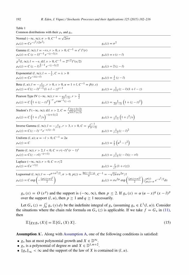
Conversely, given the density ρ∗ of Z , we can compute g∗ using (12). Some examples ofknown distributions with their g∗ are given in Table 1. Recall that g∗(z) = 0 outside the support.
Remark 5. • The necessary conditions in Proposition 4 are actually not new. Stein (LemmaVI.3 [25]) has pointed out that these are necessary for a continuous function g∗, strictlypositive on an interval (l, u), to correspond to a unique probability density function ρ∗ havingmean 0, with g∗ and ρ∗ related by (12) and (13).
• Suppose g∗ (x) = α (x − l)p for some constant α > 0 and the support of Z is (l, ∞). Then∞
0x
g∗(x)dx = ∞ if and only if p ≤ 2, and
0l
xg∗(x)
dx = −∞ if and only if 1 ≤ p.Similarly, if g∗ (x) = α (u − x)q over the support (−∞, u), 1 ≤ q ≤ 2 necessarily. Also, if
2 Nourdin and Viens proved it in the case where Z ∈ D1,2 in [17].
192 R. Eden, J. Vıquez / Stochastic Processes and their Applications 125 (2015) 182–216
Table 1Common distributions with their ρ∗ and g∗.
Normal (−∞, ∞); σ > 0, C−1=
√2πσ
ρ∗(z) = Ce−z2/(2σ2) g∗(z) = σ 2
Gamma (l, ∞); l = −rs, r > 0, s > 0, C−1= srΓ (r)
ρ∗(z) = C (z − l)r−1 e−(z−l)/s g∗(z) = s (z − l)
χ2(l, ∞); l = −v, d.f. v > 0, C−1= 2v/2Γ (v/2)
ρ∗(z) = C (z − l)v2 −1 e−(z−l)/2 g∗(z) = 2 (z − l)
Exponential (l, ∞); l = −1λ
, C = λ > 0ρ∗(z) = Ce−λ(z−l) g∗(z) =
1λ (z − l)
Beta (l, u); l = −r
r+s , r > 0, s > 0, u = 1 + l, C−1= β(r, s)
ρ∗(z) = C(z − l)r−1(1 + l − z)s−1 g∗(z) =1
r+s (z − l)(1 + l − z)
Pearson Type IV (−∞, ∞); t = −s
2(r−1), r > 3
2
ρ∗(z) = C
1 + (z − t)2−r
es tan−1(z−t) g∗(z) =1
2(r−1)
1 + (z − t)2
Student’s T (−∞, ∞); d.f. v > 2, C =
Γ ((v+1)/2)√
vπΓ (v/2)
ρ∗(z) = C
1 + z2/v−(v+1)/2
g∗(z) =v
v−1
1 + z2/v
Inverse Gamma (l, ∞); l = −
sr−1 , r > 3, s > 0, C =
sr−1
Γ (r−1)
ρ∗(z) = C(z − l)−r e−s/(z−l) g∗(z) =1
r−2 (z − l)2
Uniform (l, u); u = −l > 0, C−1= 2u
ρ∗(z) = C g∗(z) =12
u2
− z2
Pareto (l, ∞); r > 2, l < 0, C = r(−l)r (r − 1)r
ρ∗(z) = C(z − rl)−(r+1) g∗(z) =1
r−1 (z − l)(z − rl)
Laplace (−∞, ∞); r > 0, C = r/2ρ∗(z) = Ce−r |z| g∗(z) =
1r2 (1 + r |z|)
Lognormal (l, ∞); l = −eµ+σ2/2, σ > 0, p(z) =ln(z−l)−µ
σ , C−1= −
√2πσe2µ/ l
ρ∗(z) = C exp
−[p(z)+σ ]2
2
g∗(z) = σe2µ exp
[p(z)+σ ]2
2
p(z)p(z)−σ
e−s2/2ds
g∗ (x) = O (x p) and the support is (−∞, ∞), then p ≤ 2. If g∗ (x) = α (u − x)q (x − l)p
over the support (l, u), then p ≥ 1 and q ≥ 1 necessarily.
Let G∗ (z) = z
0 g∗ (y) dy be the indefinite integral of g∗ (assuming g∗ ∈ L1(l, u)). Considerthe situations where the chain rule formula on G∗ (z) is applicable. If we take f = G∗ in (11),then
E [gX g∗ (X)] = E [G∗ (X) X ] . (15)
Assumption A′. Along with Assumption A, one of the following conditions is satisfied:
• g∗ has at most polynomial growth and X ∈ D∞.• g∗ is a polynomial of degree m and X ∈ D1,m+2.• ∥g∗∥∞ < ∞ and the support of the law of X is contained in (l, u).
R. Eden, J. Vıquez / Stochastic Processes and their Applications 125 (2015) 182–216 193
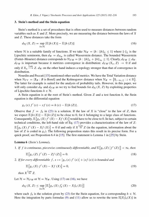
3. Stein’s method and the Stein equation
Stein’s method is a set of procedures that is often used to measure distances between randomvariables such as X and Z . More precisely, we are measuring the distance between the laws of Xand Z . These distances take the form
dH (X, Z) = suph∈H
|E [h (X)] − E [h (Z)]| (16)
where H is a suitable family of functions. If we take HW = h : ∥h∥L ≤ 1 where ∥·∥L is theLipschitz seminorm, then dW = dHW is called Wasserstein distance. The bounded Wasserstein(Fortet–Mourier) distance corresponds to H F M = h : ∥h∥L + ∥h∥∞ ≤ 1. Clearly, dF M ≤ dW .dF M is important because it metrizes convergence in distribution: dF M (Xn, Z) → 0 if and
only if XnLaw−→ Z . dW on the other hand induces a topology stronger than that of convergence in
distribution.Nourdin and Peccati [15] mentioned other useful metrics. We have the Total Variation distance
when HT V = 1B : B is Borel and the Kolmogorov distance when HK =1(−∞,z] : z ∈ R
.
The latter for example is suited for the analysis of probability tails. However, in this paper, wewill only consider dW and dF M as we try to find bounds for dH (X, Z) by exploiting propertiesof Lipschitz functions h ∈ H.
A Stein equation is at the root of Stein’s method. Given Z and a test function h, the Steinequation is the differential equation
g∗ (x) f ′ (x) − x f (x) = h (x) − E [h (Z)] . (17)
Observe that f = fh in (23) is a solution. If the law of X is “close” to the law of Z , thenwe expect E [h (X)] − E [h (Z)] to be close to 0, for h belonging to a large class of functions.Consequently, E
g∗ (X) f ′ (X) − X f (X)
would have to be close to 0. In fact, subject to certain
technical conditions, the left-hand side of Eq. (17) provides a characterization of the law of Z :
Eg∗ (X) f ′ (X) − X f (X)
= 0 if and only if X
Law= Z (in the equation, information about the
law of Z is coded in g∗). The following proposition states this result in its precise form. For aquick proof, see Proposition 6.4 in [15]. The first statement is Lemma 1 in [25] by Stein.
Lemma 6 (Stein’s Lemma).
1. If f is continuous, piecewise continuously differentiable, and Eg∗ (Z)
f ′ (Z) < ∞, then
Eg∗ (Z) f ′ (Z) − Z f (Z)
= 0. (18)
2. If for every differentiable f , x →g∗ (x) f ′ (x)
+ |x f (x)| is bounded and
Eg∗ (X) f ′ (X) − X f (X)
= 0, (19)
then XLaw= Z.
Let H = H F M or H = HW . Using (17) on (16), we have
dH (X, Z) ≤ suph∈H
E g∗ (X) f ′
h (X) − X fh (X) (20)
where each fh is the solution given by (23) for the Stein equation, for a corresponding h ∈ H.Here the integration by parts formulas (9) and (11) allow us to rewrite the term E[X fh(X)] in
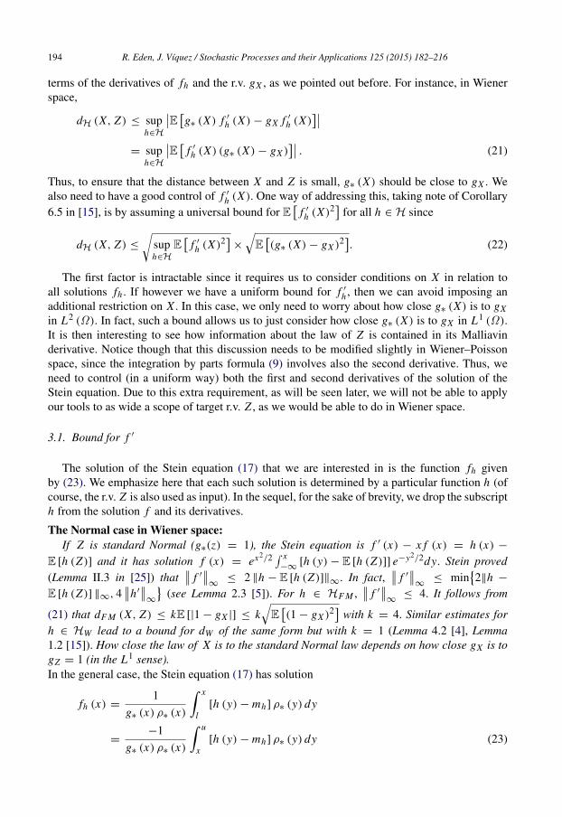
194 R. Eden, J. Vıquez / Stochastic Processes and their Applications 125 (2015) 182–216
terms of the derivatives of fh and the r.v. gX , as we pointed out before. For instance, in Wienerspace,
dH (X, Z) ≤ suph∈H
E g∗ (X) f ′
h (X) − gX f ′
h (X)
= suph∈H
E f ′
h (X) (g∗ (X) − gX ) . (21)
Thus, to ensure that the distance between X and Z is small, g∗ (X) should be close to gX . Wealso need to have a good control of f ′
h (X). One way of addressing this, taking note of Corollary6.5 in [15], is by assuming a universal bound for E
f ′
h (X)2 for all h ∈ H since
dH (X, Z) ≤
suph∈H
E
f ′
h (X)2×
E(g∗ (X) − gX )2. (22)
The first factor is intractable since it requires us to consider conditions on X in relation toall solutions fh . If however we have a uniform bound for f ′
h , then we can avoid imposing anadditional restriction on X . In this case, we only need to worry about how close g∗ (X) is to gXin L2 (Ω). In fact, such a bound allows us to just consider how close g∗ (X) is to gX in L1 (Ω).It is then interesting to see how information about the law of Z is contained in its Malliavinderivative. Notice though that this discussion needs to be modified slightly in Wiener–Poissonspace, since the integration by parts formula (9) involves also the second derivative. Thus, weneed to control (in a uniform way) both the first and second derivatives of the solution of theStein equation. Due to this extra requirement, as will be seen later, we will not be able to applyour tools to as wide a scope of target r.v. Z , as we would be able to do in Wiener space.
3.1. Bound for f ′
The solution of the Stein equation (17) that we are interested in is the function fh givenby (23). We emphasize here that each such solution is determined by a particular function h (ofcourse, the r.v. Z is also used as input). In the sequel, for the sake of brevity, we drop the subscripth from the solution f and its derivatives.
The Normal case in Wiener space:If Z is standard Normal (g∗(z) = 1), the Stein equation is f ′ (x) − x f (x) = h (x) −
E [h (Z)] and it has solution f (x) = ex2/2 x−∞
[h (y) − E [h (Z)]] e−y2/2dy. Stein proved(Lemma II.3 in [25]) that
f ′
∞≤ 2 ∥h − E [h (Z)]∥∞. In fact,
f ′
∞≤ min
2∥h −
E [h (Z)] ∥∞, 4h′
∞
(see Lemma 2.3 [5]). For h ∈ H F M ,
f ′
∞≤ 4. It follows from
(21) that dF M (X, Z) ≤ kE [|1 − gX |] ≤ kE(1 − gX )2 with k = 4. Similar estimates for
h ∈ HW lead to a bound for dW of the same form but with k = 1 (Lemma 4.2 [4], Lemma1.2 [15]). How close the law of X is to the standard Normal law depends on how close gX is togZ = 1 (in the L1 sense).In the general case, the Stein equation (17) has solution
fh (x) =1
g∗ (x) ρ∗ (x)
x
l[h (y) − mh] ρ∗ (y) dy
=−1
g∗ (x) ρ∗ (x)
u
x[h (y) − mh] ρ∗ (y) dy (23)
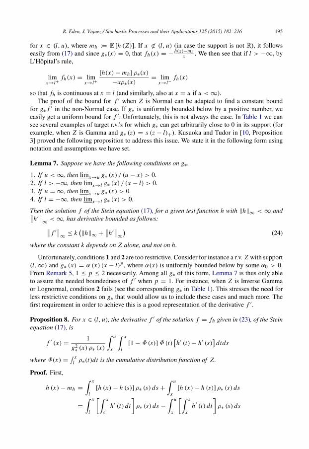
R. Eden, J. Vıquez / Stochastic Processes and their Applications 125 (2015) 182–216 195
for x ∈ (l, u), where mh := E [h (Z)]. If x ∈ (l, u) (in case the support is not R), it followseasily from (17) and since g∗(x) = 0, that fh(x) = −
h(x)−mhx . We then see that if l > −∞, by
L’Hopital’s rule,
limx→l+
fh(x) = limx→l+
[h(x) − mh] ρ∗(x)
−xρ∗(x)= lim
x→l−fh(x)
so that fh is continuous at x = l (and similarly, also at x = u if u < ∞).The proof of the bound for f ′ when Z is Normal can be adapted to find a constant bound
for g∗ f ′ in the non-Normal case. If g∗ is uniformly bounded below by a positive number, weeasily get a uniform bound for f ′. Unfortunately, this is not always the case. In Table 1 we cansee several examples of target r.v.’s for which g∗ can get arbitrarily close to 0 in its support (forexample, when Z is Gamma and g∗ (z) = s (z − l)+). Kusuoka and Tudor in [10, Proposition3] proved the following proposition to address this issue. We state it in the following form usingnotation and assumptions we have set.
Lemma 7. Suppose we have the following conditions on g∗.
1. If u < ∞, then limx→u g∗ (x) / (u − x) > 0.2. If l > −∞, then limx→l g∗ (x) / (x − l) > 0.3. If u = ∞, then limx→u g∗ (x) > 0.4. If l = −∞, then limx→l g∗ (x) > 0.
Then the solution f of the Stein equation (17), for a given test function h with ∥h∥∞ < ∞ andh′
∞< ∞, has derivative bounded as follows: f ′
∞≤ k
∥h∥∞ +
h′
∞
(24)
where the constant k depends on Z alone, and not on h.
Unfortunately, conditions 1 and 2 are too restrictive. Consider for instance a r.v. Z with support(l, ∞) and g∗ (x) = α (x) (x − l)p, where α(x) is uniformly bounded below by some α0 > 0.From Remark 5, 1 ≤ p ≤ 2 necessarily. Among all g∗ of this form, Lemma 7 is thus only ableto assure the needed boundedness of f ′ when p = 1. For instance, when Z is Inverse Gammaor Lognormal, condition 2 fails (see the corresponding g∗ in Table 1). This stresses the need forless restrictive conditions on g∗ that would allow us to include these cases and much more. Thefirst requirement in order to achieve this is a good representation of the derivative f ′.
Proposition 8. For x ∈ (l, u), the derivative f ′ of the solution f = fh given in (23), of the Steinequation (17), is
f ′ (x) =1
g2∗ (x) ρ∗ (x)
u
x
x
l[1 − Φ (s)] Φ (t)
h′ (t) − h′ (s)
dtds
where Φ(x) = x
l ρ∗(t)dt is the cumulative distribution function of Z.
Proof. First,
h (x) − mh =
x
l[h (x) − h (s)] ρ∗ (s) ds +
u
x[h (x) − h (s)] ρ∗ (s) ds
=
x
l
x
sh′ (t) dt
ρ∗ (s) ds −
u
x
s
xh′ (t) dt
ρ∗ (s) ds
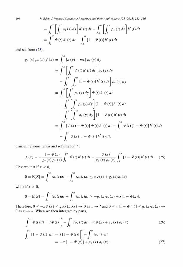
196 R. Eden, J. Vıquez / Stochastic Processes and their Applications 125 (2015) 182–216
=
x
l
t
lρ∗ (s) ds
h′ (t) dt −
u
x
u
tρ∗ (s) ds
h′ (t) dt
=
x
lΦ (t) h′ (t) dt −
u
x[1 − Φ (t)] h′ (t) dt
and so, from (23),
g∗ (x) ρ∗ (x) f (x) =
x
l[h (y) − mh] ρ∗ (y) dy
=
x
l
y
lΦ (t) h′ (t) dt
ρ∗ (y) dy
−
x
l
u
y[1 − Φ (t)] h′ (t) dt
ρ∗ (y) dy
=
x
l
x
tρ∗ (y) dy
Φ (t) h′ (t) dt
−
x
l
t
lρ∗ (y) dy
[1 − Φ (t)] h′ (t) dt
−
u
x
x
lρ∗ (y) dy
[1 − Φ (t)] h′ (t) dt
=
x
l[Φ (x) − Φ (t)] Φ (t) h′ (t) dt −
x
lΦ (t) [1 − Φ (t)] h′ (t) dt
−
u
xΦ (x) [1 − Φ (t)] h′ (t) dt.
Canceling some terms and solving for f ,
f (x) = −1 − Φ (x)
g∗ (x) ρ∗ (x)
x
lΦ (t) h′ (t) dt −
Φ (x)
g∗ (x) ρ∗ (x)
u
x[1 − Φ (t)] h′ (t) dt. (25)
Observe that if x < 0,
0 = E[Z ] =
x
ltρ∗(t)dt +
u
xtρ∗(t)dt ≤ xΦ(x) + g∗(x)ρ∗(x)
while if x > 0,
0 = E[Z ] =
x
ltρ∗(t)dt +
u
xtρ∗(t)dt ≥ −g∗(x)ρ∗(x) + x[1 − Φ(x)].
Therefore, 0 ≤ −xΦ (x) ≤ g∗(x)ρ∗(x) → 0 as x → l and 0 ≤ x [1 − Φ (x)] ≤ g∗(x)ρ∗(x) →
0 as x → u. When we then integrate by parts, x
lΦ (t) dt = tΦ (t)
xl−
x
ltρ∗ (t) dt = xΦ (x) + g∗ (x) ρ∗ (x) (26) u
x[1 − Φ (t)] dt = t [1 − Φ (t)]
ux+
u
xtρ∗ (t) dt
= −x [1 − Φ (x)] + g∗ (x) ρ∗ (x) . (27)
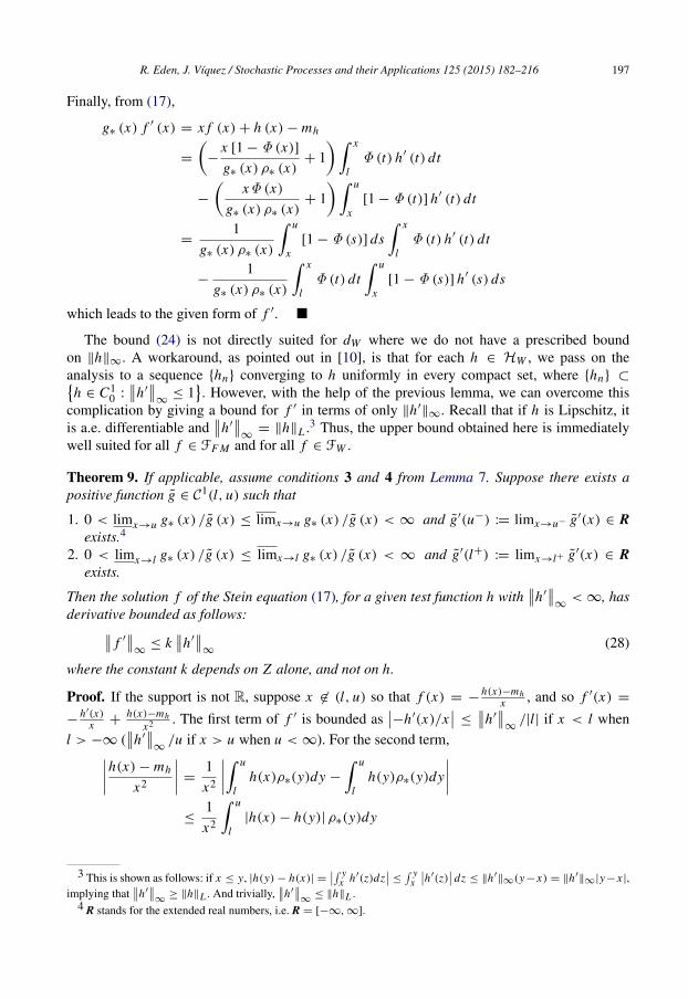
R. Eden, J. Vıquez / Stochastic Processes and their Applications 125 (2015) 182–216 197
Finally, from (17),
g∗ (x) f ′ (x) = x f (x) + h (x) − mh
=
−
x [1 − Φ (x)]g∗ (x) ρ∗ (x)
+ 1 x
lΦ (t) h′ (t) dt
−
xΦ (x)
g∗ (x) ρ∗ (x)+ 1
u
x[1 − Φ (t)] h′ (t) dt
=1
g∗ (x) ρ∗ (x)
u
x[1 − Φ (s)] ds
x
lΦ (t) h′ (t) dt
−1
g∗ (x) ρ∗ (x)
x
lΦ (t) dt
u
x[1 − Φ (s)] h′ (s) ds
which leads to the given form of f ′.
The bound (24) is not directly suited for dW where we do not have a prescribed boundon ∥h∥∞. A workaround, as pointed out in [10], is that for each h ∈ HW , we pass on theanalysis to a sequence hn converging to h uniformly in every compact set, where hn ⊂h ∈ C1
0 :h′
∞≤ 1
. However, with the help of the previous lemma, we can overcome this
complication by giving a bound for f ′ in terms of only ∥h′∥∞. Recall that if h is Lipschitz, it
is a.e. differentiable andh′
∞= ∥h∥L .3 Thus, the upper bound obtained here is immediately
well suited for all f ∈ FF M and for all f ∈ FW .
Theorem 9. If applicable, assume conditions 3 and 4 from Lemma 7. Suppose there exists apositive function g ∈ C 1(l, u) such that
1. 0 < limx→u g∗ (x) /g (x) ≤ limx→u g∗ (x) /g (x) < ∞ and g′(u−) := limx→u− g′(x) ∈ Rexists.4
2. 0 < limx→l g∗ (x) /g (x) ≤ limx→l g∗ (x) /g (x) < ∞ and g′(l+) := limx→l+ g′(x) ∈ Rexists.
Then the solution f of the Stein equation (17), for a given test function h withh′
∞< ∞, has
derivative bounded as follows: f ′
∞≤ k
h′
∞(28)
where the constant k depends on Z alone, and not on h.
Proof. If the support is not R, suppose x ∈ (l, u) so that f (x) = −h(x)−mh
x , and so f ′(x) =
−h′(x)
x +h(x)−mh
x2 . The first term of f ′ is bounded as−h′(x)/x
≤h′
∞/|l| if x < l when
l > −∞ (h′
∞/u if x > u when u < ∞). For the second term,h(x) − mh
x2
=1
x2
u
lh(x)ρ∗(y)dy −
u
lh(y)ρ∗(y)dy
≤
1
x2
u
l|h(x) − h(y)| ρ∗(y)dy
3 This is shown as follows: if x ≤ y, |h(y) − h(x)| = y
x h′(z)dz ≤
yx
h′(z) dz ≤ ∥h′
∥∞(y−x) = ∥h′∥∞|y−x |,
implying thath′∞
≥ ∥h∥L . And trivially,h′∞
≤ ∥h∥L .4 R stands for the extended real numbers, i.e. R = [−∞, ∞].
198 R. Eden, J. Vıquez / Stochastic Processes and their Applications 125 (2015) 182–216
≤∥h∥L
x2
u
l|x − y|ρ∗(y)dy
≤∥h∥L
x2 (|x | + E[|Z |]) = ∥h∥L
1|x |
+E[|Z |]
x2
.
If x < l when l > −∞, the second factor is bounded by 1/|l| + E[|Z |]/ l2 (we have a similarbound when u < ∞).
Assume now that x is in the support of Z . Note that from Proposition 8,
f ′ (x) ≤
2h′
∞
g2∗ (x) ρ∗ (x)
u
x[1 − Φ (s)] ds
x
lΦ (t) dt. (29)
Fix l ′ and u′ s.t. l < l ′ < 0 < u′ < u. Since g∗(x)ρ∗(x) is continuous and strictly positiveon [l ′, u′
], it attains its minimum m := inf[l ′,u′] g∗(x)ρ∗(x) > 0 on this compact set. Also by
continuity of the density M := sup[l ′,u′] ρ∗(x) < ∞, and g∗ (x) =g∗(x)ρ∗(x)
ρ∗(x)≥
mM > 0 on
l ′, u′, so g2
∗(x)ρ∗(x) ≥m2
M . By the continuity and positivity of I1(x) := u
x [1 − Φ (s)] dsand I2(x) :=
xl Φ (t) dt we conclude that K := sup[l ′,u′] (I1(x) ∨ I2(x)) < ∞. By (29),
| f ′(x)| ≤2M K 2
m2
h′
∞onl ′, u′
.
Since l ′ and u′ were arbitrarily chosen, we only need to prove now that limx→l f ′ (x)
≤
k1∥h′∥∞ and limx→u
f ′ (x) ≤ k2∥h′
∥∞ for some finite constants k1 and k2. Due to thesymmetry of the arguments it suffices to prove just one of these limits. Suppose l ′ was chosensmall enough so that g ∈ C 1
l, l ′
, and for some constants 0 < c ≤ C < ∞, cg∗ (x) ≤ g (x) ≤
Cg∗ (x) onl, l ′
.
• Case 1: l > −∞.
We show that the limit of the right-hand side of (29) is finite as x → l. Note that in thiscase,
ux [1 − Φ (s)] ds = g∗ (x) ρ∗ (x) − x [1 − Φ (x)] → |l|. By L’Hopital’s rule,
limx→l
f ′ (x) ≤ 2
h′
∞|l| lim
x→l
C x
l Φ (t) dt
g (x) g∗ (x) ρ∗ (x)
≤ 2h′
∞|l| C lim
x→l
Φ (x)
−x g (x) ρ∗ (x) + g′ (x) g∗ (x) ρ∗ (x)
≤ 2h′
∞|l| C lim
x→l
Φ (x)−cx + g′ (x)
g∗ (x) ρ∗ (x)
≤2h′
∞|l| C
g′l+− cl
limx→l
ρ∗ (x)
−xρ∗ (x)=
2h′
∞C
g′l+− cl
.
Since gl+
:= limz→l+ g(z) = 0 and g ≥ 0, we may assume l ′ is small enough so g′≥ 0 on
l, l ′. Consequently, g′
l+
= cl < 0.
• Case 2: l = −∞.
Since limx→−∞g∗ (x) > 0, we may suppose l ′ is small enough so that for some constant
m0 > 0, g∗ (x) ≥ m0 over−∞, l ′
.
R. Eden, J. Vıquez / Stochastic Processes and their Applications 125 (2015) 182–216 199
limx→−∞
f ′ (x) ≤ 2∥h′
∥∞ limx→−∞
g∗ (x) ρ∗ (x) − x [1 − Φ (x)]
x−∞
Φ (t) dt
g2∗ (x) ρ∗ (x)
≤ 2h′
∞
lim
x→−∞
x−∞
Φ (t) dt
m0+ lim
x→−∞
−x x−∞
Φ (t) dt
g2∗ (x) ρ∗ (x)
= 2
h′
∞lim
x→−∞
|x | x−∞
Φ(t)dt
g2∗(x)ρ∗(x)
.
There are two subcases to consider depending on the behavior of g(x) as x → −∞. Fromthe continuity of g and the existence of g′(l+), L := limx→−∞ g(x) necessarily exists. IfL < ∞, then limx→−∞
g(x)|x |
= 0. If L = ∞, then by L’Hopital’s rule, limx→−∞g(x)|x |
=
− limx→−∞ g′(x) = −g′(l+). In either case, limx→−∞g(x)|x |
exists.
– Subcase 1: limx→−∞g(x)|x |
= ∞
Note that by (26), x−∞
Φ(t)dt = xΦ(x) + g∗(x)ρ∗(x) ≤ g∗(x)ρ∗(x) so
|x | x−∞
Φ(t)dt
g2∗(x)ρ∗(x)
≤ C|x |g∗(x)ρ∗(x)
g(x)g∗(x)ρ∗(x)= C
|x |
g(x).
Therefore
limx→−∞
f ′ (x) ≤ 2
h′
∞C lim
x→−∞
|x |
g(x)= 0 < ∞.
– Subcase 2: limx→−∞g(x)|x |
< ∞
Similarly from (26),
|x | x−∞
Φ(t)dt
g2∗(x)ρ∗(x)
≤
x−∞
|x |
|t | g∗(t)ρ∗(t)dt
m0g∗(x)ρ∗(x)≤
x−∞
g∗(t)ρ∗(t)dt
m0g∗(x)ρ∗(x).
Therefore,
limx→−∞
f ′ (x) ≤
2∥h′∥∞
m0lim
x→−∞
x−∞
g∗(t)ρ∗(t)dt
g∗(x)ρ∗(x)≤
2∥h′∥∞
m0lim
x→−∞
g∗(x)ρ∗(x)
−xρ∗(x)
≤2∥h′
∥∞
m0lim
x→−∞
g(x)
c|x |< ∞.
The proof that limx→u f ′ (x)
≤ k2∥h′∥∞ for some k2 < ∞ is similar.
Note that if g∗ is uniformly bounded below in a neighborhood of l > −∞ (or for u < ∞)then condition 2 (1 in the case of u) from Theorem 9 is not required (see discussion beforeLemma 7). In the statement of the previous theorem, we can take g = g∗ if g∗ is continuouslydifferentiable (at least locally C 1 close to the endpoints of the support), and in this case theconditions are trivially met. In other words, if we can check that g∗ ∈ C 1(l, u) then bound (28) isautomatically true (given the existence of g′(u−) and g′(l+)). These new conditions are met byall r.v.’s in the Exponential family, Pearson family, and practically any other r.v. whose densityis C 1 and is strictly positive in its support. If g∗ is not continuously differentiable, we can stillget the bound but we are required to approximate g∗ by a continuously differentiable function gnear the endpoints of the support. For example, consider the Laplace distribution where g∗(x) =1c2 (1 + c|x |) (see Table 1). In this case g∗ is differentiable everywhere except at 0. Therefore we
200 R. Eden, J. Vıquez / Stochastic Processes and their Applications 125 (2015) 182–216
can choose g(x) = g∗(x) for all x ∈−∞, l ′
∪u′, ∞
(with −∞ < l ′ < 0 < u′ < ∞) and
g(x) = φ(x) on (l ′, u′) where φ is a smooth function such that g is differentiable at l ′ and u′.
Assumption B. We have the following conditions on g∗.
1. For some positive g ∈ C 1 (l, u),(a) 0 < limx→u g∗ (x) /g (x) ≤ limx→u g∗ (x) /g (x) < ∞.(b) 0 < limx→l g∗ (x) /g (x) ≤ limx→l g∗ (x) /g (x) < ∞.(c) g′(l+) and g′(u−) exist.
2. If u = ∞, then limx→u g∗ (x) > 0.3. If l = −∞, then limx→l g∗ (x) > 0.
3.2. Bound for f ′′
We reiterate that when we refer to a solution f of the Stein equation, we mean the solution fhgiven by (23). It is in fact determined by a test function h, but we will drop here the subscript hfor brevity.
For our convergence in distribution results in Wiener–Poisson space, we need a boundednessresult for f ′′. The existence of f ′′ demands more conditions on g∗ such as differentiability, whichis understandable since we are requiring greater regularity in the solution of the Stein equation.In this setting, the existence of f ′′ will also immediately force most conditions of Theorem 9to be satisfied. If we want to work with dW or dF M , we need to consider Lipschitz functions h,and for any such test function, we can only hope for it to be differentiable almost everywhere.Consequently, f ′′ must be understood in the almost everywhere sense, i.e., f ′′ is a version of thesecond derivative of f such that wherever the second derivative does not exist, f ′′ will have avalue of 0.
Before setting out to find a bound, we point out the unfortunate fact that our results here willnot apply to as wide a range of target r.v. Z as what happened for the first derivative. Morespecifically, we will not be able to give a finite bound for
f ′′ (x) when l > −∞ or u < ∞,
as we were able to do for f ′ (x)
in Theorem 9. See the paragraph before Remark 10 for acounterexample: a bounded Lipschitz function h such that if the support of Z is (l, ∞) R,then f ′′(x) does not tend to a finite limit as x → l. A similar counterexample can be constructedfor a r.v. Z with support (−∞, u) R, or with support (l, u) R.
First, we make preliminary computations on f ′′. Differentiating (17) gives us the secondderivative
f ′′ (x) =x − g′
∗ (x)
g∗ (x)f ′ (x) +
1g∗ (x)
f (x) +1
g∗ (x)h′ (x)
which, after considering the form of f in Eq. (25) and of f ′ given in Proposition 8, reduces to
f ′′ (x)
=A (x)
xl Φ (t) h′ (t) dt + B (x)
ux [1 − Φ (s)] h′ (s) ds + g2
∗ (x) ρ∗ (x) h′ (x)
g3∗ (x) ρ∗ (x)
(30)
where, with the help of (26) and (27),
A (x) =x − g′
∗ (x) u
x[1 − Φ (s)] ds − g∗ (x) (1 − Φ (x))
= g∗ (x) ρ∗ (x)x − g′
∗ (x)− Q(x) (1 − Φ (x)) (31)
R. Eden, J. Vıquez / Stochastic Processes and their Applications 125 (2015) 182–216 201
B (x) = −x − g′
∗ (x) x
lΦ (t) dt − g∗ (x)Φ (x)
= g∗ (x) ρ∗ (x)g′∗ (x) − x
− Q(x)Φ (x) . (32)
Here, we defined for our convenience the function Q as
Q(x) = x2− xg′
∗(x) + g∗(x). (33)
Let d (x) = g3∗ (x) ρ∗ (x) and n (x) = f ′′ (x) d (x), the indicated denominator and numerator,
respectively, of f ′′ (x). As x → l, both d (x) and n (x) tend to 0. If h′ happens to bedifferentiable, then by L’Hopital’s rule, limx→l f ′′ (x) = limx→l n′ (x) /d ′ (x). It can be shownthat
A′ (x) =2 − g′′
∗ (x) u
x[1 − Φ (s)] ds (34)
and B ′ (x) = −2 − g′′
∗ (x) x
l Φ (t) dt . Therefore
n′ (x) = A′ (x)
x
lΦ (t) h′ (t) dt + A (x)Φ (x) h′ (x) + B ′ (x)
×
u
x[1 − Φ (s)] h′ (s) ds − B (x) [1 − Φ (x)] h′ (x)
+−xg∗ (x) ρ∗ (x) + g′
∗ (x) g∗ (x) ρ∗ (x)
h′ (x) + g2∗ (x) ρ∗ (x) h′′ (x)
=2 − g′′
∗ (x) u
x[1 − Φ (s)] ds
x
lΦ (t) h′ (t) dt −
2 − g′′
∗ (x)
×
x
lΦ (t) dt
u
x[1 − Φ (s)] h′ (s) ds + [A (x)Φ (x) − B (x) (1 − Φ (x))
−x − g′
∗ (x)
g∗ (x) ρ∗ (x)
h′ (x) + g2∗ (x) ρ∗ (x) h′′ (x)
=2 − g′′
∗ (x)
g2∗ (x) ρ∗ (x) f ′ (x) + 0 · h′ (x) + g2
∗ (x) ρ∗ (x) h′′ (x)
and so
limx→l
f ′′ (x) = limx→l
2 − g′′
∗ (x)
g2∗ (x) ρ∗ (x) f ′ (x) + g2
∗ (x) ρ∗ (x) h′′ (x)2g′
∗ (x) − x
g2∗ (x) ρ∗ (x)
= limx→l
2 − g′′∗ (x)
2g′∗ (x) − x
f ′ (x) + limx→l
h′′ (x)
2g′∗ (x) − x
.
Define the function h (x) =43 (x − l)3/2 on (l, 0), h (x) =
43 |l|3/2 on [0, ∞) and h (x) = 0
on (−∞, l]. This function is clearly Lipschitz. Note that h′′ (x) =1
√x−l
on (l, 0). We now
consider the same assumptions from Theorem 9 and see that limx→l f ′ (x)
≤ kh′
∞and
limx→lh′′(x)
2g′∗(x)−x = ∞. We have thus found a Lipschitz function h for which limx→l
f ′′ (x) =
∞.
Remark 10. From the above discussion we cannot expect to have a universal bound on thesecond derivative of f unless the support of the target r.v. is (−∞, ∞). This is consistent with theknown NP bound in Wiener–Poisson space developed in [29], where Z was Normal and hencehad (−∞, ∞) for support. For the rest of this subsection, we will then assume that l = −∞ andu = ∞.
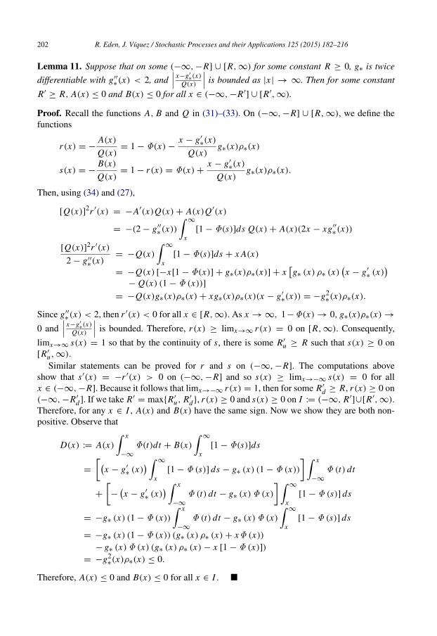
202 R. Eden, J. Vıquez / Stochastic Processes and their Applications 125 (2015) 182–216
Lemma 11. Suppose that on some (−∞, −R] ∪ [R, ∞) for some constant R ≥ 0, g∗ is twice
differentiable with g′′∗(x) < 2, and
x−g′∗(x)
Q(x)
is bounded as |x | → ∞. Then for some constant
R′≥ R, A(x) ≤ 0 and B(x) ≤ 0 for all x ∈ (−∞, −R′
] ∪ [R′, ∞).
Proof. Recall the functions A, B and Q in (31)–(33). On (−∞, −R] ∪ [R, ∞), we define thefunctions
r(x) = −A(x)
Q(x)= 1 − Φ(x) −
x − g′∗(x)
Q(x)g∗(x)ρ∗(x)
s(x) = −B(x)
Q(x)= 1 − r(x) = Φ(x) +
x − g′∗(x)
Q(x)g∗(x)ρ∗(x).
Then, using (34) and (27),
[Q(x)]2r ′(x) = −A′(x)Q(x) + A(x)Q′(x)
= −(2 − g′′∗(x))
∞
x[1 − Φ(s)]ds Q(x) + A(x)(2x − xg′′
∗(x))
[Q(x)]2r ′(x)
2 − g′′∗(x)
= −Q(x)
∞
x[1 − Φ(s)]ds + x A(x)
= −Q(x) [−x[1 − Φ(x)] + g∗(x)ρ∗(x)] + xg∗ (x) ρ∗ (x)
x − g′
∗ (x)
− Q(x) (1 − Φ (x))]= −Q(x)g∗(x)ρ∗(x) + xg∗(x)ρ∗(x)(x − g′
∗(x)) = −g2∗(x)ρ∗(x).
Since g′′∗(x) < 2, then r ′(x) < 0 for all x ∈ [R, ∞). As x → ∞, 1−Φ(x) → 0, g∗(x)ρ∗(x) →
0 and x−g′
∗(x)
Q(x)
is bounded. Therefore, r(x) ≥ limx→∞ r(x) = 0 on [R, ∞). Consequently,
limx→∞ s(x) = 1 so that by the continuity of s, there is some R′u ≥ R such that s(x) ≥ 0 on
[R′u, ∞).Similar statements can be proved for r and s on (−∞, −R]. The computations above
show that s′(x) = −r ′(x) > 0 on (−∞, −R] and so s(x) ≥ limx→−∞ s(x) = 0 for allx ∈ (−∞, −R]. Because it follows that limx→−∞ r(x) = 1, then for some R′
d ≥ R, r(x) ≥ 0 on(−∞, −R′
d ]. If we take R′= maxR′
u, R′
d, r(x) ≥ 0 and s(x) ≥ 0 on I := (−∞, R′]∪[R′, ∞).
Therefore, for any x ∈ I , A(x) and B(x) have the same sign. Now we show they are both non-positive. Observe that
D(x) := A(x)
x
−∞
Φ(t)dt + B(x)
∞
x[1 − Φ(s)]ds
=
x − g′
∗ (x) ∞
x[1 − Φ (s)] ds − g∗ (x) (1 − Φ (x))
x
−∞
Φ (t) dt
+
−x − g′
∗ (x) x
−∞
Φ (t) dt − g∗ (x)Φ (x)
∞
x[1 − Φ (s)] ds
= −g∗ (x) (1 − Φ (x))
x
−∞
Φ (t) dt − g∗ (x)Φ (x)
∞
x[1 − Φ (s)] ds
= −g∗ (x) (1 − Φ (x)) (g∗ (x) ρ∗ (x) + xΦ (x))
− g∗ (x)Φ (x) (g∗ (x) ρ∗ (x) − x [1 − Φ (x)])= −g2
∗(x)ρ∗(x) ≤ 0.
Therefore, A(x) ≤ 0 and B(x) ≤ 0 for all x ∈ I .
R. Eden, J. Vıquez / Stochastic Processes and their Applications 125 (2015) 182–216 203
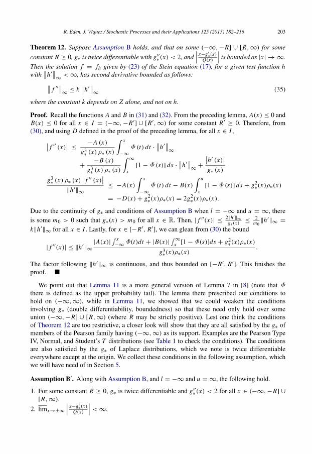
Theorem 12. Suppose Assumption B holds, and that on some (−∞, −R] ∪ [R, ∞) for some
constant R ≥ 0, g∗ is twice differentiable with g′′∗(x) < 2, and
x−g′∗(x)
Q(x)
is bounded as |x | → ∞.
Then the solution f = fh given by (23) of the Stein equation (17), for a given test function hwith
h′
∞< ∞, has second derivative bounded as follows: f ′′
∞≤ k
h′
∞(35)
where the constant k depends on Z alone, and not on h.
Proof. Recall the functions A and B in (31) and (32). From the preceding lemma, A(x) ≤ 0 andB(x) ≤ 0 for all x ∈ I = (−∞, −R′
] ∪ [R′, ∞) for some constant R′≥ 0. Therefore, from
(30), and using D defined in the proof of the preceding lemma, for all x ∈ I , f ′′ (x) ≤
−A (x)
g3∗ (x) ρ∗ (x)
x
−∞
Φ (t) dt ·h′
∞
+−B (x)
g3∗ (x) ρ∗ (x)
∞
x[1 − Φ (s)] ds ·
h′
∞+
h′ (x)
g∗ (x)
g3∗ (x) ρ∗ (x)
f ′′ (x)
∥h′∥∞
≤ −A(x)
x
−∞
Φ (t) dt − B(x)
u
x[1 − Φ (s)] ds + g2
∗(x)ρ∗(x)
= −D(x) + g2∗(x)ρ∗(x) = 2g2
∗(x)ρ∗(x).
Due to the continuity of g∗ and conditions of Assumption B when l = −∞ and u = ∞, thereis some m0 > 0 such that g∗(x) > m0 for all x ∈ R. Then, | f ′′(x)| ≤
2∥h′∥∞
g∗(x)≤
2m0
∥h′∥∞ =
k∥h′∥∞ for all x ∈ I . Lastly, for x ∈ [−R′, R′
], we can glean from (30) the bound
| f ′′(x)| ≤ ∥h′∥∞
|A(x)| x−∞
Φ(t)dt + |B(x)|
∞
x [1 − Φ(s)]ds + g2∗(x)ρ∗(x)
g3∗(x)ρ∗(x)
.
The factor following ∥h′∥∞ is continuous, and thus bounded on [−R′, R′
]. This finishes theproof.
We point out that Lemma 11 is a more general version of Lemma 7 in [8] (note that Φthere is defined as the upper probability tail). The lemma there prescribed our conditions tohold on (−∞, ∞), while in Lemma 11, we showed that we could weaken the conditionsinvolving g∗ (double differentiability, boundedness) so that these need only hold over someunion (−∞, −R] ∪ [R, ∞) (where R may be strictly positive). Lest one think the conditionsof Theorem 12 are too restrictive, a closer look will show that they are all satisfied by the g∗ ofmembers of the Pearson family having (−∞, ∞) as its support. Examples are the Pearson TypeIV, Normal, and Student’s T distributions (see Table 1 to check the conditions). The conditionsare also satisfied by the g∗ of Laplace distributions, which we note is twice differentiableeverywhere except at the origin. We collect these conditions in the following assumption, whichwe will have need of in Section 5.
Assumption B′. Along with Assumption B, and l = −∞ and u = ∞, the following hold.
1. For some constant R ≥ 0, g∗ is twice differentiable and g′′∗(x) < 2 for all x ∈ (−∞, −R] ∪
[R, ∞).
2. limx→±∞
x−g′∗(x)
Q(x)
< ∞.
204 R. Eden, J. Vıquez / Stochastic Processes and their Applications 125 (2015) 182–216
4. NP bound in Wiener space
From the results in Section 3.1 all solutions f = fh given by (23), of the Stein equation,belong to a set FH = f ∈ C 1(l, u) : ∥ f ′
∥∞ ≤ k. While the constant k will not depend on thespecific test function h used, it may still be driven by general characteristics of the members ofH, the family of test functions used. See the beginning of Section 3.1 for different choices of kunder various families H, when Z is standard Normal.
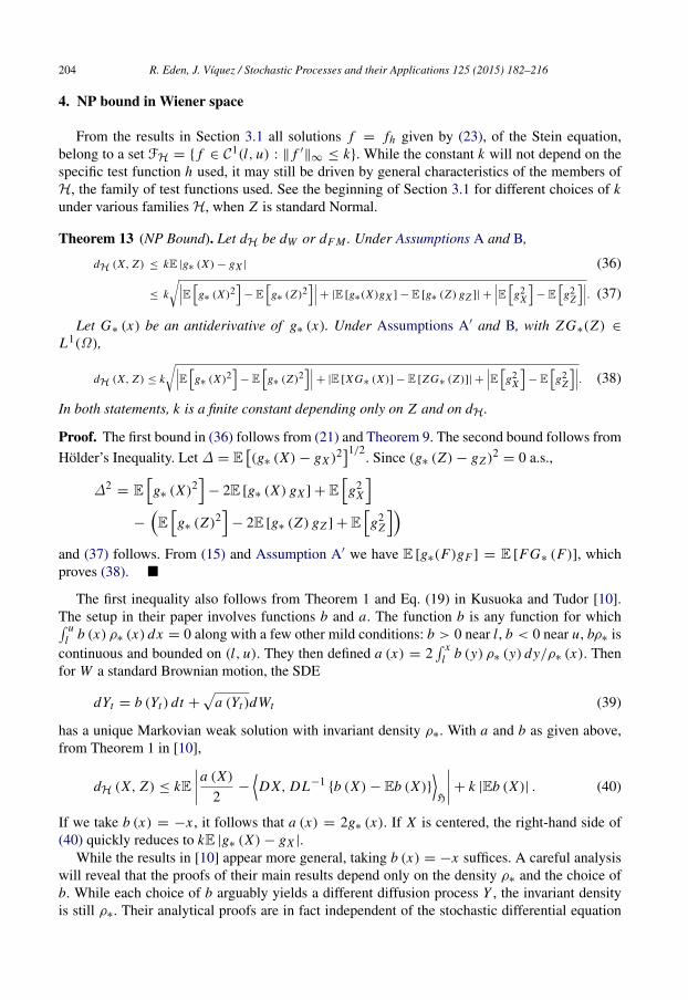
Theorem 13 (NP Bound). Let dH be dW or dF M . Under Assumptions A and B,
dH (X, Z) ≤ kE |g∗ (X) − gX | (36)
≤ k
E g∗ (X)2
− Eg∗ (Z)2
+ |E [g∗(X)gX ] − E [g∗ (Z) gZ ]| +
E g2X
− E
g2
Z
. (37)
Let G∗ (x) be an antiderivative of g∗ (x). Under Assumptions A′ and B, with ZG∗(Z) ∈
L1(Ω),
dH (X, Z) ≤ k
E g∗ (X)2
− Eg∗ (Z)2
+ |E [XG∗ (X)] − E [ZG∗ (Z)]| +
E g2X
− E
g2
Z
. (38)
In both statements, k is a finite constant depending only on Z and on dH.
Proof. The first bound in (36) follows from (21) and Theorem 9. The second bound follows fromHolder’s Inequality. Let ∆ = E
(g∗ (X) − gX )21/2
. Since (g∗ (Z) − gZ )2= 0 a.s.,
∆2= E
g∗ (X)2
− 2E [g∗ (X) gX ] + E
g2
X
−
Eg∗ (Z)2
− 2E [g∗ (Z) gZ ] + E
g2
Z
and (37) follows. From (15) and Assumption A′ we have E [g∗(F)gF ] = E [FG∗ (F)], whichproves (38).
The first inequality also follows from Theorem 1 and Eq. (19) in Kusuoka and Tudor [10].The setup in their paper involves functions b and a. The function b is any function for which u
l b (x) ρ∗ (x) dx = 0 along with a few other mild conditions: b > 0 near l, b < 0 near u, bρ∗ iscontinuous and bounded on (l, u). They then defined a (x) = 2
xl b (y) ρ∗ (y) dy/ρ∗ (x). Then
for W a standard Brownian motion, the SDE
dYt = b (Yt ) dt +
a (Yt )dWt (39)
has a unique Markovian weak solution with invariant density ρ∗. With a and b as given above,from Theorem 1 in [10],
dH (X, Z) ≤ kEa (X)
2−
DX, DL−1
b (X) − Eb (X)H
+ k |Eb (X)| . (40)
If we take b (x) = −x , it follows that a (x) = 2g∗ (x). If X is centered, the right-hand side of(40) quickly reduces to kE |g∗ (X) − gX |.
While the results in [10] appear more general, taking b (x) = −x suffices. A careful analysiswill reveal that the proofs of their main results depend only on the density ρ∗ and the choice ofb. While each choice of b arguably yields a different diffusion process Y , the invariant densityis still ρ∗. Their analytical proofs are in fact independent of the stochastic differential equation
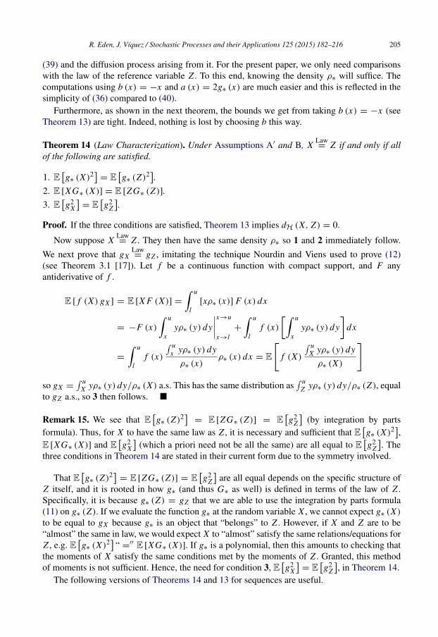
R. Eden, J. Vıquez / Stochastic Processes and their Applications 125 (2015) 182–216 205
(39) and the diffusion process arising from it. For the present paper, we only need comparisonswith the law of the reference variable Z . To this end, knowing the density ρ∗ will suffice. Thecomputations using b (x) = −x and a (x) = 2g∗ (x) are much easier and this is reflected in thesimplicity of (36) compared to (40).
Furthermore, as shown in the next theorem, the bounds we get from taking b (x) = −x (seeTheorem 13) are tight. Indeed, nothing is lost by choosing b this way.
Theorem 14 (Law Characterization). Under Assumptions A′ and B, XLaw= Z if and only if all
of the following are satisfied.
1. Eg∗ (X)2
= Eg∗ (Z)2.
2. E [XG∗ (X)] = E [ZG∗ (Z)].
3. Eg2
X
= E
g2
Z
.
Proof. If the three conditions are satisfied, Theorem 13 implies dH (X, Z) = 0.
Now suppose XLaw= Z . They then have the same density ρ∗ so 1 and 2 immediately follow.
We next prove that gXLaw= gZ , imitating the technique Nourdin and Viens used to prove (12)
(see Theorem 3.1 [17]). Let f be a continuous function with compact support, and F anyantiderivative of f .
E [ f (X) gX ] = E [X F (X)] =
u
l[xρ∗ (x)] F (x) dx
= −F (x)
u
xyρ∗ (y) dy
x→u
x→l+
u
lf (x)
u
xyρ∗ (y) dy
dx
=
u
lf (x)
ux yρ∗ (y) dy
ρ∗ (x)ρ∗ (x) dx = E
f (X)
uX yρ∗ (y) dy
ρ∗ (X)
so gX = u
X yρ∗ (y) dy/ρ∗ (X) a.s. This has the same distribution as u
Z yρ∗ (y) dy/ρ∗ (Z), equalto gZ a.s., so 3 then follows.
Remark 15. We see that Eg∗ (Z)2
= E [ZG∗ (Z)] = Eg2
Z
(by integration by parts
formula). Thus, for X to have the same law as Z , it is necessary and sufficient that Eg∗ (X)2,
E [XG∗ (X)] and Eg2
X
(which a priori need not be all the same) are all equal to E
g2
Z
. The
three conditions in Theorem 14 are stated in their current form due to the symmetry involved.
That Eg∗ (Z)2
= E [ZG∗ (Z)] = Eg2
Z
are all equal depends on the specific structure of
Z itself, and it is rooted in how g∗ (and thus G∗ as well) is defined in terms of the law of Z .Specifically, it is because g∗ (Z) = gZ that we are able to use the integration by parts formula(11) on g∗ (Z). If we evaluate the function g∗ at the random variable X , we cannot expect g∗ (X)
to be equal to gX because g∗ is an object that “belongs” to Z . However, if X and Z are to be“almost” the same in law, we would expect X to “almost” satisfy the same relations/equations forZ , e.g. E
g∗ (X)2 “ =
′′ E [XG∗ (X)]. If g∗ is a polynomial, then this amounts to checking thatthe moments of X satisfy the same conditions met by the moments of Z . Granted, this methodof moments is not sufficient. Hence, the need for condition 3, E
g2
X
= E
g2
Z
, in Theorem 14.
The following versions of Theorems 14 and 13 for sequences are useful.
206 R. Eden, J. Vıquez / Stochastic Processes and their Applications 125 (2015) 182–216
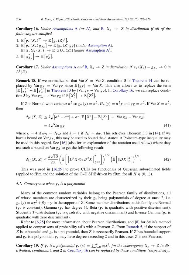
Corollary 16. Under Assumptions A (or A′) and B, Xn → Z in distribution if all of thefollowing are satisfied.
1. Eg∗ (Xn)2
→ Eg∗ (Z)2.
2. Eg∗ (Xn) gXn
→ E [g∗ (Z) gZ ] (under Assumption A).
E [XnG∗ (Xn)] → E [ZG∗ (Z)] (under Assumption A′).
3. Eg2
Xn
→ E
g2
Z
.
Corollary 17. Under Assumptions A and B, Xn → Z in distribution if g∗ (Xn) − gXn → 0 inL1(Ω).
Remark 18. If we normalize so that Var X = Var Z , condition 3 in Theorem 14 can be re-placed by Var gX = Var gZ since E [gX ] = Var X . This also allows us to replace the termE g2
X
− E
g2
Z
in Theorem 13 by |Var gX − Var gZ |. In Corollary 16, we can replace condi-tion 3 by Var gXn → Var gZ if E
X2
n
→ E
Z2.
If Z is Normal with variance σ 2 so g∗ (y) = σ 2, G∗ (y) = σ 2 y and gZ = σ 2. If Var X = σ 2,then
dH (X, Z) ≤ kσ 4 − σ 4
+ σ 2E X2
− E
Z2+ |Var gX − Var gZ |
= k
Var gX (41)
where k = 4 if dH = dF M and k = 1 if dH = dW . This retrieves Theorem 3.3 in [14]. If wehave a bound on Var gX , this may be used to bound the distance. A Poincare-type inequality maybe used in this regard. See [16] (also for an explanation of the notation used below) where theyuse such a bound on Var gX to get the following result:
dH (X, Z) ≤k√
102σ
ED2 X ⊗1 D2 X
2
H⊗2
1/2 E∥DX∥
4H
1/2. (42)
This was used in [16,29] to prove CLTs for functionals of Gaussian subordinated fields(applied to fBm and the solution of the O–U SDE driven by fBm, for all H ∈ (0, 1)).
4.1. Convergence when g∗ is a polynomial
Many of the common random variables belong to the Pearson family of distributions, allof whose members are characterized by their g∗ being polynomials of degree at most 2, i.e.g∗ (y) = αy2
+βy +γ in the support of Z . Some member distributions in this family are Normal(g∗ is constant), Gamma (g∗ has degree 1), Beta (g∗ is quadratic with positive discriminant),Student’s T -distribution (g∗ is quadratic with negative discriminant) and Inverse Gamma (g∗ isquadratic with zero discriminant).
Refer to [6,25] for more information about Pearson distributions, and [8] for Stein’s methodapplied to comparisons of probability tails with a Pearson Z . From Remark 5, if the support ofZ is unbounded and g∗ is a polynomial, then Z is necessarily Pearson. If Z has bounded supportand g∗ is a polynomial, g∗ may have degree exceeding 2 and in this case, Z is not Pearson.
Corollary 19. If g∗ is a polynomial g∗ (x) =m
k=0 ak xk , for the convergence Xn → Z in dis-tribution, conditions 1 and 2 in Corollary 16 can be replaced by these conditions (respectively):
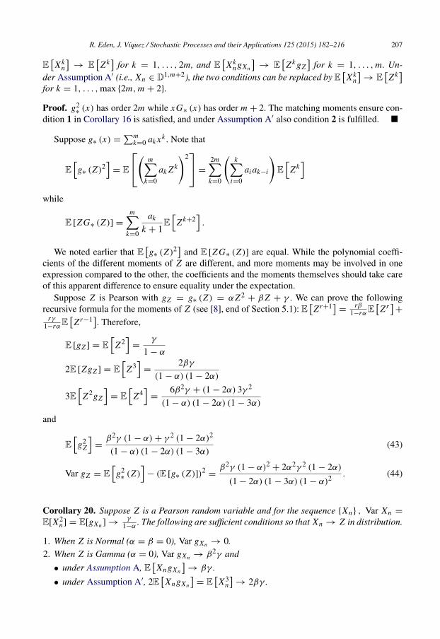
R. Eden, J. Vıquez / Stochastic Processes and their Applications 125 (2015) 182–216 207
EX k
n
→ E
Z k
for k = 1, . . . , 2m, and EX k
ngXn
→ E
Z k gZ
for k = 1, . . . , m. Un-
der Assumption A′ (i.e., Xn ∈ D1,m+2), the two conditions can be replaced by EX k
n
→ E
Z k
for k = 1, . . . , max 2m, m + 2.
Proof. g2∗ (x) has order 2m while xG∗ (x) has order m + 2. The matching moments ensure con-
dition 1 in Corollary 16 is satisfied, and under Assumption A′ also condition 2 is fulfilled.
Suppose g∗ (x) =m
k=0 ak xk . Note that
Eg∗ (Z)2
= E
mk=0
ak Z k
2 =
2mk=0
k
i=0
ai ak−i
E
Z k
while
E [ZG∗ (Z)] =
mk=0
ak
k + 1E
Z k+2.
We noted earlier that Eg∗ (Z)2 and E [ZG∗ (Z)] are equal. While the polynomial coeffi-
cients of the different moments of Z are different, and more moments may be involved in oneexpression compared to the other, the coefficients and the moments themselves should take careof this apparent difference to ensure equality under the expectation.
Suppose Z is Pearson with gZ = g∗ (Z) = αZ2+ βZ + γ . We can prove the following
recursive formula for the moments of Z (see [8], end of Section 5.1): EZr+1
=
rβ1−rα
EZr+
rγ1−rα
EZr−1
. Therefore,
E [gZ ] = E
Z2
=γ
1 − α
2E [ZgZ ] = E
Z3
=2βγ
(1 − α) (1 − 2α)
3E
Z2gZ
= E
Z4
=6β2γ + (1 − 2α) 3γ 2
(1 − α) (1 − 2α) (1 − 3α)
and
Eg2
Z
=
β2γ (1 − α) + γ 2 (1 − 2α)2
(1 − α) (1 − 2α) (1 − 3α)(43)
Var gZ = Eg2∗ (Z)
− (E [g∗ (Z)])2
=β2γ (1 − α)2
+ 2α2γ 2 (1 − 2α)
(1 − 2α) (1 − 3α) (1 − α)2 . (44)
Corollary 20. Suppose Z is a Pearson random variable and for the sequence Xn , Var Xn =
E[X2n] = E[gXn ] →
γ1−α
. The following are sufficient conditions so that Xn → Z in distribution.
1. When Z is Normal (α = β = 0), Var gXn → 0.2. When Z is Gamma (α = 0), Var gXn → β2γ and
• under Assumption A, EXngXn
→ βγ .
• under Assumption A′, 2EXngXn
= E
X3
n
→ 2βγ .
208 R. Eden, J. Vıquez / Stochastic Processes and their Applications 125 (2015) 182–216
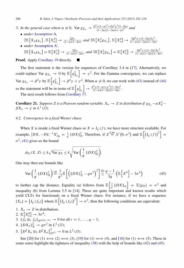
3. In the general case where α = 0, Var gXn →β2γ (1−α)2
+2α2γ 2(1−2α)
(1−2α)(1−3α)(1−α)2 and
• under Assumption A,
2EXngXn
,EX3
n
→
2βγ(1−α)(1−2α)
, and 3EX2
ngXn
,EX4
n
→
6β2γ+(1−2α)3γ 2
(1−α)(1−2α)(1−3α).
• under Assumption A′,
2EXngXn
= E
X3
n
→
2βγ(1−α)(1−2α)
, and 3EX2
ngXn
= E
X4
n
→
6β2γ+(1−2α)3γ 2
(1−α)(1−2α)(1−3α).
Proof. Apply Corollary 19 directly.
The first statement is the version for sequences of Corollary 3.4 in [17]. Alternatively, we
could replace Var gXn → 0 by Eg2
Xn
→ γ 2. For the Gamma convergence, we can replace
Var gXn → β2γ by Eg2
Xn
→ β2γ + γ 2. When α = 0, we can work with (43) instead of (44)
so the statement will be in terms of Eg2
Xn
→
β2γ (1−α)+γ 2(1−2α)2
(1−α)(1−2α)(1−3α).
The next result follows from Corollary 17.
Corollary 21. Suppose Z is a Pearson random variable. Xn → Z in distribution if gXn −αX2n −
β Xn → γ in L1 (Ω).
4.2. Convergence in a fixed Wiener chaos
When X is inside a fixed Wiener chaos so X = Iq ( f ), we have more structure available. For
example,DX, −DL−1 X
H
=1q ∥DX∥
2H. Therefore, if Z
Law= N
0, σ 2
and E
Iq ( f )
2=
σ 2, (41) gives us the bound
dH (X, Z) ≤ k
Var gX ≤ k
Var
1q
∥DX∥2H
.
One may then use bounds like
Var
1q
∥DX∥2H
(a)=
1
q2E
∥DX∥2H − qσ 2
2
(b)≤
q − 13q
E
X4
− 3σ 4
(45)
to further cap the distance. Equality (a) follows from E
1q ∥DX∥H
= E [gX ] = σ 2 and
inequality (b) from Lemma 3.5 in [14]. These are quite important and known results whichyield CLTs for functionals on a fixed Wiener chaos. For instance, if we have a sequence
Xn =
Iq ( fn)
where E
Iq ( fn)2
→ σ 2, then the following conditions are equivalent:
1. Xn → Z in distribution;2. E
X4
n
→ 3σ 4;
3. ∥ fn ⊗r fn∥H⊗(2q−2r) → 0 for all r = 1, . . . , q − 1;4. ∥DXn∥
2H → qσ 2 in L2 (Ω);
5.D2 Xn ⊗1 D2 Xn
2H⊗2 → 0 in L2 (Ω).
See [20] for (1) ⇐⇒ (2) ⇐⇒ (3), [19] for (1) ⇐⇒ (4), and [16] for (1) ⇐⇒ (5). These insome sense highlight the tightness of inequality (38) with the help of bounds like (42) and (45).
R. Eden, J. Vıquez / Stochastic Processes and their Applications 125 (2015) 182–216 209
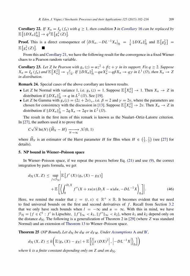
Corollary 22. If Xn = Iq ( fn) with q ≥ 1, then condition 3 in Corollary 16 can be replaced byE∥DXn∥
4H
→ q2E
g2∗ (Z)
.
Proof. This is a direct consequence ofDXn, −DL−1 Xn
H
=1q ∥DXn∥
2H and E
g2
Z
=
Eg2∗ (Z)
.
From this and Corollary 21, we have the following result for the convergence in a fixed Wienerchaos to a Pearson random variable.
Corollary 23. Let Z be Pearson with g∗ (z) = αz2+ βz + γ in its support. Fix q ≥ 2. Suppose
Xn = Iq ( fn) and EX2
n
→
γ1−α
. If ∥DXn∥2H −qαX2
n −qβ Xn → qγ in L1 (Ω), then Xn → Zin distribution.
Remark 24. Special cases of the above corollary are known results.
• Let Z be Normal with variance 1, i.e. g∗ (z) = 1. Suppose EX2
n
→ 1. Then Xn → Z in
distribution if ∥DXn∥2H → q in L2 (Ω). See [19].
• Let Z be Gamma with g∗(z) = (2z + 2v)+, i.e. β = 2 and γ = 2v, where the parameters arechosen for consistency with the discussion in [13]. Suppose E
X2
n
→ 2v. Then Xn → Z in
distribution if ∥DXn∥2H − 2q Xn → 2qv in L2 (Ω).
The result in the first item of this remark is known as the Nualart–Ortiz-Latorre criterion.In [27], the authors used it to prove that
C√
N ln(N ) HN − H
−−−−→N→∞
N (0, 1)
where HN is an estimator of the Hurst parameter H for fBm when H ∈ 1
3 , 12
(see [27] for
details).
5. NP bound in Wiener–Poisson space
In Wiener–Poisson space, if we repeat the process before Eq. (21) and use (9), the correctintegration by parts formula, we get
dH (X, Z) ≤ supf ∈FH
E f ′ (X) (g∗ (X) − gX )
+E Dz X
0f ′′(X + xu)x(Dz X − u)du, −DL−1 X
H
. (46)
Here, we remind the reader that z = (t, x) ∈ R+× R. It becomes evident that we need
to find universal bounds on the first and second derivatives of f . Recall from Section 3.2that we only have such bounds when l = −∞ and u = ∞. With this in mind, we haveFH = f ∈ C 1
: f ′ is Lipschitz, ∥ f ′∥∞ < k1, ∥ f ′′
∥∞ < k2, where k1 and k2 depend only onthe distance dH. The following is a generalization of Theorem 2 in [29] (where Z was standardNormal) and an extension of Theorem 13 to Wiener–Poisson space.
Theorem 25 (NP Bound). Let dH be dW or dF M . Under Assumptions A and B′,
dH (X, Z) ≤ k
E |g∗ (X) − gX | + E
x (DX)2 , −DL−1 X
H
where k is a finite constant depending only on Z and on dH.
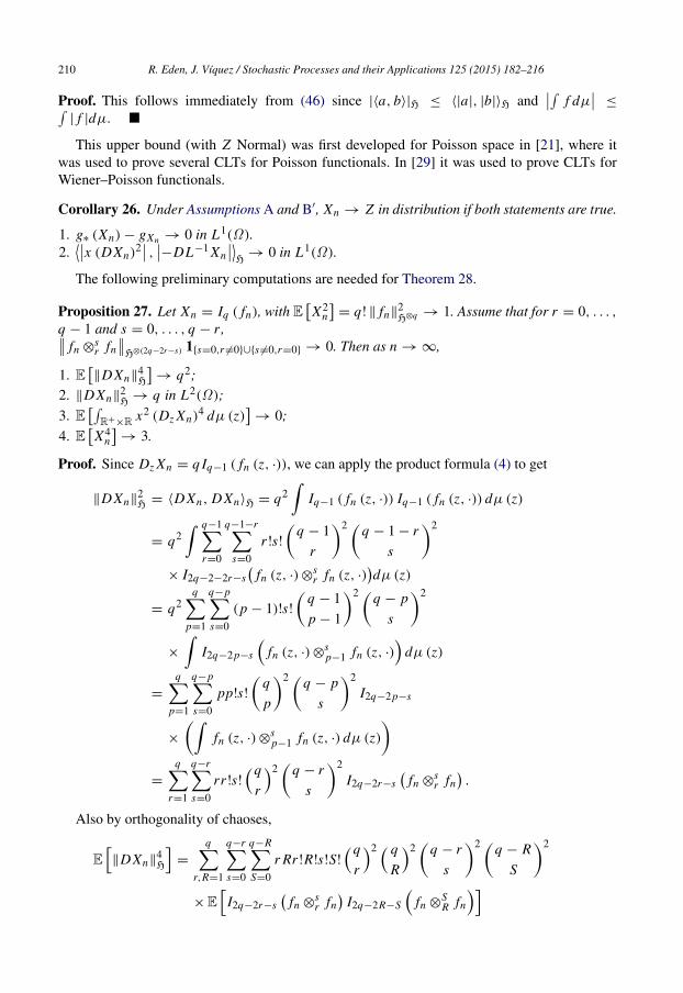
210 R. Eden, J. Vıquez / Stochastic Processes and their Applications 125 (2015) 182–216
Proof. This follows immediately from (46) since |⟨a, b⟩|H ≤ ⟨|a|, |b|⟩H and f dµ
≤| f |dµ.
This upper bound (with Z Normal) was first developed for Poisson space in [21], where itwas used to prove several CLTs for Poisson functionals. In [29] it was used to prove CLTs forWiener–Poisson functionals.
Corollary 26. Under Assumptions A and B′, Xn → Z in distribution if both statements are true.
1. g∗ (Xn) − gXn → 0 in L1(Ω).2.x (DXn)2
, −DL−1 Xn
H→ 0 in L1(Ω).
The following preliminary computations are needed for Theorem 28.
Proposition 27. Let Xn = Iq ( fn), with EX2
n
= q! ∥ fn∥
2H⊗q → 1. Assume that for r = 0, . . . ,
q − 1 and s = 0, . . . , q − r , fn ⊗sr fn
H⊗(2q−2r−s) 1s=0,r=0∪s=0,r=0 → 0. Then as n → ∞,
1. E∥DXn∥
4H
→ q2;
2. ∥DXn∥2H → q in L2(Ω);
3. E
R+×R x2 (Dz Xn)4 dµ (z)
→ 0;
4. EX4
n
→ 3.
Proof. Since Dz Xn = q Iq−1 ( fn (z, ·)), we can apply the product formula (4) to get
∥DXn∥2H = ⟨DXn, DXn⟩H = q2
Iq−1 ( fn (z, ·)) Iq−1 ( fn (z, ·)) dµ (z)
= q2 q−1
r=0
q−1−rs=0
r !s!
q − 1
r
2 q − 1 − r
s
2
× I2q−2−2r−s
fn (z, ·) ⊗sr fn (z, ·)
dµ (z)
= q2q
p=1
q−ps=0
(p − 1)!s!
q − 1p − 1
2 q − p
s
2
×
I2q−2p−s
fn (z, ·) ⊗
sp−1 fn (z, ·)
dµ (z)
=
qp=1
q−ps=0
pp!s!
q
p
2 q − p
s
2
I2q−2p−s
×
fn (z, ·) ⊗
sp−1 fn (z, ·) dµ (z)
=
qr=1
q−rs=0
rr !s!q
r
2
q − r
s
2
I2q−2r−s
fn ⊗sr fn
.
Also by orthogonality of chaoses,
E∥DXn∥
4H
=
qr,R=1
q−rs=0
q−RS=0
r Rr !R!s!S!
q
r
2 q
R
2
q − r
s
2 q − R
S
2
×E
I2q−2r−s
fn ⊗sr fn
I2q−2R−S
fn ⊗
SR fn
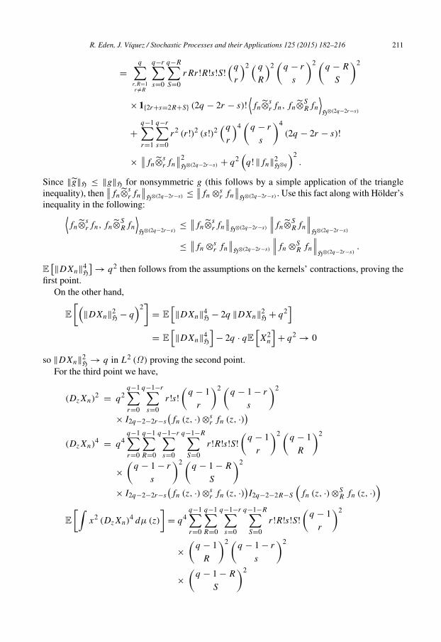
R. Eden, J. Vıquez / Stochastic Processes and their Applications 125 (2015) 182–216 211
=
qr,R=1r=R
q−rs=0
q−RS=0
r Rr !R!s!S!
q
r
2 q
R
2
q − r
s
2 q − R
S
2
× 12r+s=2R+S (2q − 2r − s)!
fn⊗sr fn, fn⊗S
R fn
H⊗(2q−2r−s)
+
q−1r=1
q−rs=0
r2 (r !)2 (s!)2q
r
4
q − r
s
4
(2q − 2r − s)!
× fn⊗s
r fn2
H⊗(2q−2r−s) + q2
q! ∥ fn∥2H⊗q
2.
Since ∥g∥H ≤ ∥g∥H for nonsymmetric g (this follows by a simple application of the triangleinequality), then
fn⊗sr fn
H⊗(2q−2r−s) ≤
fn ⊗sr fn
H⊗(2q−2r−s) . Use this fact along with Holder’s
inequality in the following:fn⊗s
r fn, fn⊗SR fn
H⊗(2q−2r−s)
≤ fn⊗s
r fn
H⊗(2q−2r−s)
fn⊗SR fn
H⊗(2q−2r−s)
≤ fn ⊗
sr fn
H⊗(2q−2r−s)
fn ⊗SR fn
H⊗(2q−2r−s)
.
E∥DXn∥
4H
→ q2 then follows from the assumptions on the kernels’ contractions, proving the
first point.On the other hand,
E
∥DXn∥2H − q
2
= E∥DXn∥
4H − 2q ∥DXn∥
2H + q2
= E
∥DXn∥
4H
− 2q · qE
X2
n
+ q2
→ 0
so ∥DXn∥2H → q in L2 (Ω) proving the second point.
For the third point we have,
(Dz Xn)2= q2
q−1r=0
q−1−rs=0
r !s!
q − 1
r
2 q − 1 − r
s
2
× I2q−2−2r−s
fn (z, ·) ⊗sr fn (z, ·)
(Dz Xn)4
= q4q−1r=0
q−1R=0
q−1−rs=0
q−1−RS=0
r !R!s!S!
q − 1
r
2 q − 1R
2
×
q − 1 − r
s
2 q − 1 − R
S
2
× I2q−2−2r−s
fn (z, ·) ⊗sr fn (z, ·)
I2q−2−2R−S
fn (z, ·) ⊗
SR fn (z, ·)
E
x2 (Dz Xn)4 dµ (z)
= q4
q−1r=0
q−1R=0
q−1−rs=0
q−1−RS=0
r !R!s!S!
q − 1
r
2
×
q − 1
R
2 q − 1 − r
s
2
×
q − 1 − R
S
2
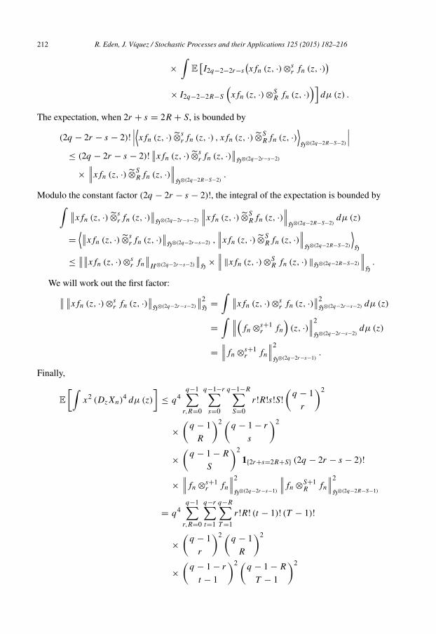
212 R. Eden, J. Vıquez / Stochastic Processes and their Applications 125 (2015) 182–216
×
EI2q−2−2r−s
x fn (z, ·) ⊗
sr fn (z, ·)
× I2q−2−2R−S
x fn (z, ·) ⊗
SR fn (z, ·)
dµ (z) .
The expectation, when 2r + s = 2R + S, is bounded by
(2q − 2r − s − 2)!
x fn (z, ·)⊗sr fn (z, ·) , x fn (z, ·)⊗S
R fn (z, ·)H⊗(2q−2R−S−2)
≤ (2q − 2r − s − 2)!
x fn (z, ·)⊗sr fn (z, ·)
H⊗(2q−2r−s−2)
×
x fn (z, ·)⊗SR fn (z, ·)
H⊗(2q−2R−S−2)
.
Modulo the constant factor (2q − 2r − s − 2)!, the integral of the expectation is bounded by x fn (z, ·)⊗sr fn (z, ·)
H⊗(2q−2r−s−2)
x fn (z, ·)⊗SR fn (z, ·)
H⊗(2q−2R−S−2)
dµ (z)
=
x fn (z, ·)⊗sr fn (z, ·)
H⊗(2q−2r−s−2) ,
x fn (z, ·)⊗SR fn (z, ·)
H⊗(2q−2R−S−2)
H
≤x fn (z, ·) ⊗
sr fn
H⊗(2q−2r−s−2)
H
×
∥x fn (z, ·) ⊗SR fn (z, ·) ∥H⊗(2q−2R−S−2)
H
.
We will work out the first factor: x fn (z, ·) ⊗sr fn (z, ·)
H⊗(2q−2r−s−2)
2H
=
x fn (z, ·) ⊗sr fn (z, ·)
2H⊗(2q−2r−s−2) dµ (z)
=
fn ⊗s+1r fn
(z, ·)
2
H⊗(2q−2r−s−2)dµ (z)
=
fn ⊗s+1r fn
2
H⊗(2q−2r−s−1).
Finally,
E
x2 (Dz Xn)4 dµ (z)
≤ q4
q−1r,R=0
q−1−rs=0
q−1−RS=0
r !R!s!S!
q − 1
r
2
×
q − 1
R
2 q − 1 − r
s
2
×
q − 1 − R
S
2
12r+s=2R+S (2q − 2r − s − 2)!
×
fn ⊗s+1r fn
2
H⊗(2q−2r−s−1)
fn ⊗S+1R fn
2
H⊗(2q−2R−S−1)
= q4q−1
r,R=0
q−rt=1
q−RT =1
r !R! (t − 1)! (T − 1)!
×
q − 1
r
2 q − 1R
2
×
q − 1 − r
t − 1
2 q − 1 − R
T − 1
2
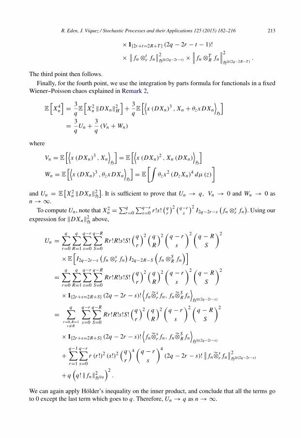
R. Eden, J. Vıquez / Stochastic Processes and their Applications 125 (2015) 182–216 213
× 12r+t=2R+T (2q − 2r − t − 1)!
× fn ⊗
tr fn
2H⊗(2q−2r−t) ×
fn ⊗TR fn
2
H⊗(2q−2R−T ).
The third point then follows.
Finally, for the fourth point, we use the integration by parts formula for functionals in a fixedWiener–Poisson chaos explained in Remark 2,
E
X4n
=
3qE
X2n ∥DXn∥
2H
+
3qE
x (DXn)3 , Xn + θz x DXn
H
=
3q
Un +3q
(Vn + Wn)
where
Vn = E
x (DXn)3 , Xn
H
= E
x (DXn)2 , Xn (DXn)
H
Wn = E
x (DXn)3 , θz x DXn
H
= E
θz x2 (Dz Xn)4 dµ (z)
and Un = E
X2
n ∥DXn∥2H
. It is sufficient to prove that Un → q, Vn → 0 and Wn → 0 as
n → ∞.
To compute Un , note that X2n =
qr=0
q−rs=0 r !s!
qr
2 q−rs
2I2q−2r−s
fn ⊗
sr fn
. Using our
expression for ∥DXn∥2H above,
Un =
qr=0
qR=1
q−rs=0
q−RS=0
Rr !R!s!S!
q
r
2 q
R
2
q − r
s
2 q − R
S
2
×E
I2q−2r−s
fn ⊗sr fn
I2q−2R−S
fn ⊗
SR fn
=
qr=0
qR=1
q−rs=0
q−RS=0
Rr !R!s!S!
q
r
2 q
R
2
q − r
s
2 q − R
S
2
× 12r+s=2R+S (2q − 2r − s)!
fn⊗sr fn, fn⊗S
R fn
H⊗(2q−2r−s)
=
qr=0,R=1
r=R
q−rs=0
q−RS=0
Rr !R!s!S!
q
r
2 q
R
2
q − r
s
2 q − R
S
2
× 12r+s=2R+S (2q − 2r − s)!
fn⊗sr fn, fn⊗S
R fn
H⊗(2q−2r−s)
+
q−1r=1
q−rs=0
r (r !)2 (s!)2q
r
4
q − r
s
4
(2q − 2r − s)! fn⊗s
r fn2
H⊗(2q−2r−s)
+ q
q! ∥ fn∥2H⊗q
2.
We can again apply Holder’s inequality on the inner product, and conclude that all the terms goto 0 except the last term which goes to q . Therefore, Un → q as n → ∞.
214 R. Eden, J. Vıquez / Stochastic Processes and their Applications 125 (2015) 182–216
Observe that
|Vn| ≤ Ex (DXn)2
H
∥Xn (DXn)∥H
≤
Ex (DXn)2
2H
E∥Xn (DXn)∥2
H
=
E
x2 (Dz Xn)4 dµ (z)
E∥Xn (DXn)∥2
H
.
Note that
E∥Xn (DXn)∥2
H
= E
X2
n ∥DXn∥2H
= Un → q.
From the third point, E
R+×R x2 (Dz Xn)4 dµ (z)
→ 0 so Vn → 0 as n → ∞.Finally for Wn ,
|Wn| = E
θz x2 (Dz Xn)4 dµ (z)
≤ E
x2 (Dz Xn)4 dµ (z)
−→ 0.
Putting them together we get the fourth point: E[X4n] → 3 as n → ∞.
In Wiener space, convergence in a fixed Wiener chaos to a standard normal distribution ischaracterized by the convergence of the fourth moments to 3 or of the convergence of the normof certain contractions to 0 (see the list preceding Corollary 22). We would then like to see if thesame situation holds in Wiener–Poisson space. At this point, this appears to be an open question.We then finish with the following theorem which shows convergence in distribution and of thefourth moments to 3 if certain contractions converge to 0.
Theorem 28. Suppose Assumptions A and B′ hold. Let Xn = Iq ( fn), with EX2
n
=
q! ∥ fn∥2H⊗q → 1. Assume that for r = 0, . . . , q − 1 and s = 0, . . . , q −
r, fn ⊗
sr fn
H⊗(2q−2r−s) 1s=0,r=0∪s=0,r=0 → 0. Then as n → ∞,
• E[X4n] → 3.
• Xn → N (0, 1) in distribution.
Proof. The first assertion is the fourth point in Proposition 27. For the second point, we referto Corollary 26 to see that it suffices to prove g∗ (Xn) − gXn → 0 in L2 (Ω) and
|x | (DXn)2 ,
|DXn|H
→ 0 in L1(Ω) as n → ∞. These are immediate when we note that
g∗(Xn) − gXn = 1 −1q
∥DXn∥2H → 0 in L2(Ω) (by point 2 of Proposition 27)
and
E
|x | (DXn)2 , |DXn|
H
≤ E
x (DXn)2
H∥DXn∥H
≤
Ex (DXn)2
2H
E∥DXn∥
2H
=
E
x2 (DXn)4 dµ
qE
X2
n
→ 0
(by point 3 of Proposition 27).
R. Eden, J. Vıquez / Stochastic Processes and their Applications 125 (2015) 182–216 215
Acknowledgments
We are deeply grateful to our respective Ph.D. advisors, Frederi Viens and Fabrice Baudoin,for their very helpful comments in making this paper, and primarily for introducing us toMalliavin calculus. We would also like to thank David Nualart for his valuable insights, andthe anonymous referees for their careful reading and astute observations.
References
[1] D. Applebaum, Levy Processes and Stochastic Calculus, Cambridge University Press, Cambridge, 2004.[2] F. Baudoin, C. Ouyang, S. Tindel, Upper bounds for the density of solutions of stochastic differential equations
driven by fractional Brownian motions, Ann. Inst. H. Poincare 50 (1) (2014) 111–135.[3] S. Bourguin, C. Tudor, Cramer theorem for Gamma random variables, Electron. Comm. Probab. 16 (2011) 365–378.[4] S. Chatterjee, A new method of Normal approximation, Ann. Probab. 36 (4) (2008) 1584–1610.[5] L. Chen, Q.-M. Shao, Stein’s method for normal approximation, in: An Introduction to Stein’s Method, in: Lect.
Notes Ser. Inst. Math. Sci. Natl. Univ. Singap., Singapore Univ. Press, Singapore, 2005, pp. 1–59.[6] P. Diaconis, S. Zabell, Closed form summation for classical distributions: variations on a theme of De Moivre,
Statist. Sci. 14 (3) (1991) 284–302.[7] G. Di Nunno, On orthogonal polynomials and the Malliavin derivative for Levy stochastic measures, Anal. Probab.
Sem. Congr. 16 (2008) 55–69.[8] R. Eden, F. Viens, General upper and lower tail estimates using Malliavin calculus and Stein’s equations, in: Seminar
on Stochastic Analysis, Random Fields and Applications VII—Progress in Probability. Vol. 67, 2013, pp. 55–84.[9] K. Ito, Spectral type of the shift transformation of differential processes with stationary increments, Trans. Amer.
Math. Soc. 81 (2) (1956) 252–263.[10] S. Kusuoka, C. Tudor, Stein method for invariant measures of diffusions via Malliavin calculus, Stochastic Process.
Appl. 122 (4) (2012) 1627–1651.[11] Y. Lee, H. Shih, The product formula of multiple Levy–Ito integrals, Bull. Inst. Math. Acad. Sin. 32 (2) (2004)
71–95.[12] S. Noreddine, I. Nourdin, On the Gaussian approximation of vector-valued multiple integrals, J. Multivariate Anal.
102 (6) (2011) 1008–1017.[13] I. Nourdin, G. Peccati, Noncentral convergence of multiple integrals, Ann. Probab. 37 (4) (2009) 1412–1426.[14] I. Nourdin, G. Peccati, Stein’s method meets Malliavin calculus: a short survey with new estimates, in: J. Duan,
S. Luo, C. Wang (Eds.), Recent Development in Stochastic Dynamics and Stochastic Analysis, World Scientific,2009.
[15] I. Nourdin, G. Peccati, Stein’s method on Wiener chaos, Probab. Theory Related Fields 145 (1) (2009) 75–118.[16] I. Nourdin, G. Peccati, G. Reinert, Second order Poincare inequalities and CLTs on Wiener space, J. Funct. Anal.
257 (2) (2009) 593–609.[17] I. Nourdin, F. Viens, Density formula and concentration inequalities with Malliavin calculus, Electron. J. Probab.
14 (2009) 2287–2309.[18] D. Nualart, The Malliavin Calculus and Related Topics, second ed., Springer Verlag, Berlin, 2006.[19] D. Nualart, S. Ortiz-Latorre, Central limit theorems for multiple stochastic integrals and Malliavin calculus,
Stochastic Process. Appl. 118 (2008) 614–628.[20] D. Nualart, G. Peccati, Central limit theorems for sequences of multiple stochastic integrals, Ann. Probab. 33 (1)
(2005) 177–193.[21] G. Peccati, J.L. Sole, M.S. Taqqu, F. Utzet, Stein’s method and normal approximation of Poisson functionals, Ann.
Probab. 38 (2) (2010) 443–478.[22] K. Sato, Levy Processes and Infinitely Divisible Distributions, Cambridge University Press, Cambridge, 1999.[23] J.L. Sole, F. Utzet, J. Vives, Canonical Levy process and Malliavin calculus, Stochastic Process. Appl. 117 (2)
(2007) 165–187.[24] J.L. Sole, F. Utzet, J. Vives, Chaos expansions and Malliavin calculus for Levy processes, in: Stochastic Analysis
and Applications—Abel Symposia, vol. 2, Springer, 2007, pp. 595–612.[25] C. Stein, Approximate Computation of Expectations, in: Institute of Mathematical Statistics Lecture Notes—
Monograph Series, vol. 7, 1986.[26] C. Tudor, Asymptotic Cramer’s theorem and analysis on Wiener space, in: Seminaire de Probabilite XLIII,
in: Lecture Notes in Mathematics, 2011, pp. 309–325.
216 R. Eden, J. Vıquez / Stochastic Processes and their Applications 125 (2015) 182–216
[27] C. Tudor, F. Viens, Variations and estimators for the selfsimilarity order through Malliavin calculus, Ann. Probab.6 (2009) 2093–2134.
[28] F. Viens, Stein’s lemma, Malliavin Calculus, and tail bounds, with application to polymer fluctuation exponent,Stochastic Process. Appl. 119 (2009) 3671–3698.
[29] J.J. Viquez, On the second order Poincare inequality and CLT on Wiener–Poisson space.Preprint http://arxiv.org/abs/1104.1837.