notes - the department of mathematics at virginia tech · notes for numerical analysis math 5466 b...

1

Notes for Numerical Analysis

Math 5466

by

S. Adjerid

Virginia Polytechnic Institute

and State University

(A Rough Draft)

Contents

1 Polynomial Interpolation 5

1.1 Review . . . . . . . . . . . . . . . . . . . . . . . . . . . . . . . 51.2 Introduction . . . . . . . . . . . . . . . . . . . . . . . . . . . . 61.3 Lagrange Interpolation . . . . . . . . . . . . . . . . . . . . . . 71.4 Interpolation error and convergence . . . . . . . . . . . . . . . 11

1.4.1 Interpolation error . . . . . . . . . . . . . . . . . . . . 121.4.2 Convergence . . . . . . . . . . . . . . . . . . . . . . . . 15

1.5 Interpolation at Chebyshev points . . . . . . . . . . . . . . . . 191.6 Hermite interpolation . . . . . . . . . . . . . . . . . . . . . . . 26

1.6.1 Lagrange form of Hermite interpolation polynomials . . 261.6.2 Newton form of Hermite interpolation polynomial . . . 281.6.3 Hermite interpolation error . . . . . . . . . . . . . . . . 30

1.7 Spline Interpolation . . . . . . . . . . . . . . . . . . . . . . . . 321.7.1 Piecewise Lagrange interpolation . . . . . . . . . . . . 321.7.2 Cubic spline interpolation . . . . . . . . . . . . . . . . 341.7.3 Convergence of cubic splines . . . . . . . . . . . . . . . 461.7.4 B-splines . . . . . . . . . . . . . . . . . . . . . . . . . . 55

1.8 Interpolation in multiple dimensions . . . . . . . . . . . . . . . 581.9 Least-squares Approximations . . . . . . . . . . . . . . . . . . 58

3

4 CONTENTS

Chapter 1

Polynomial Interpolation

1.1 Review

Mean-value theorem: Let f 2 C[a; b] and di�erentiable on (a; b) thenthere exists c 2 (a; b) such that

f 0(c) =f(b)� f(a)

b� a:

Weighted Mean-value theorem: If f 2 C[a; b] and g(x) > 0 on [a; b],then there exists c 2 (a; b) such that

Z b

a

f(x)g(x)dx = f(c)

Z b

a

g(x)dx:

Rolle's theorem: If f 2 C[a; b], di�erentiable on (a; b) and f(a) = f(b),then there exists c 2 (a; b) such that f 0(c) = 0.

Generalized Rolle's theorem: If f 2 C[a; b], n+1 times di�erentiable on(a; b) and admits n + 2 zeros in [a; b], then there exists c 2 (a; b) such thatf (n+1)(c) = 0.

Intermediate value theorem: If f 2 C[a; b] such that f(a) 6= f(b), thenfor each y between f(a) and f(b) there exists c 2 (a; b) such that f(c) = y.

5

6 CHAPTER 1. POLYNOMIAL INTERPOLATION

1.2 Introduction

From the Webster dictionary the de�nition of interpolation reads as follows:\Interpolation is the act of introducing something, especially, spurious andforeign, the act of calculating values of functions between values alreadyknown"

Our goal is approximate a set of data points or a function by a simplerpolynomial function. Given a set of data points xi; i = 0; 1; � � �n; xi 6=xj; if i 6= j we would like to construct a polynomial pm(x) such that

p(k)m (xi) = f (k)(xi); i = 0; 1; � � �m; k = 0; 1; � � �ni; with n =mXi=0

ni � 1:

Lagrange Interpolation: ni = 0, m � 1 , pn(xi) = f(xi); i = 0; 1; � � � ; n

Taylor Interpolation: n0 > 1, m = 0 , p(k)n (x0) = f (k)(x0); k = 0; 1; � � � ; n0.

Hermite Interpolation: ni � 1, m � 1 , p(k)n (xi) = f (k)(xi); i = 0; 1; � � � ; m;

k = 0; 1; � � �ni.

Why Interpolation? For instance interpolation is used to approximateintegrals

bZa

f(x)dx �Z b

a

pm(x)dx

derivatives

f (k)(x) � p(k)m (x)

and plays a major role in approximating di�erential equations.

Taylor interpolation:

We �rst study Taylor polynomials de�ned as

pn(x) = f(x0)+ (x� x0)f0

(x0)+(x� x0)

2

2f (2)(x0)+ � � �+ (x� x0)

n

n!f (n)(x0):

1.3. LAGRANGE INTERPOLATION 7

The interpolation error or remainder formula in Taylor expansions is writtenas

f(x)� pn(x) =(x� x0)

n+1

(n+ 1)!f (n+1)(�)

Example: f(x) = sin(x); x0 = 0

p2n+1(x) =nX

k=0

(�1)k x2k+1

(2k + 1)!

The interpolation error can be written as

jsin(x)� p2n+1(x)j = jxj2n+3

(2n+ 3)!jcos(�)j < jxj2n+3

(2n+ 3)!

On the interval 0 < x < 1=2 the interpolation error is bounded as

jsin(x)� p2n+1(x)j < 1

22n+3(2n+ 3)!:

1.3 Lagrange Interpolation

Lagrange form:

Given a set of points (xi; f(xi)); i = 0; 1; 2; � � �n; xj 6= xi we de�ne theLagrange coeÆcient polynomials li(x); i = 0; 1; � � �n: such as

li(xj) =

(1; if i = j

0; otherwise

and is de�ned as

li(x) =(x� x0)(x� x1) � � � (x� xi�1)(x� xi+1) � � � (x� xn)

(xi � x0)(xi � x1) � � � (xi � xi�1)(xi � xi+1) � � � (xi � xn):

The Lagrange form of the interpolation polynomial is

pn(x) =nXi=0

f(xi)li(x)


Example: Let us consider the data set x = [0; 1; 2]; f = [�2;�1; 2]

l0(x) =(x� 1)(x� 2)

(�1)(�2) = (x2 � 3x+ 2)=2

l1(x) =x(x� 2)

(1)(�1) = �x2 + 2x

l2(x) =x(x� 1)

(2)(1)= (x2 � x)=2

p2(x) = �2l0(x)� l1(x) + 2l2(x) = x2 � 2

Example:

f(x) = cos(x)5 using 8 points x = [0; 1; 2; 3; 4; 5; 6; 7] and 14 points xi =i � 0:5; i = 0; 2; � � �14

A Matlab example

x=[0 1 2 3 4 5 6 7];

y=cos(x).^5;

c = polyfit(x,y,length(x)-1);

xi = 0:0.1:7;

zi = cos(xi).^5;

yi =polyval(c,xi);

subplot(2,1,1)

title('Interpolation')

plot(xi,yi,'-.',xi,zi,x,y,'*');

subplot(2,1,2)

title('Interpolation Error')

plot(xi,zi-yi,x,zeros(1,length(x)),'-*');

Newton form and divided di�erences:

We develop a procedure to compute a0; a1; � � � ; an such that the interpola-tion polynomial has the form

pn(x) = a0 + a1(x� x0) + a2(x� x0)(x� x1) + � � �+ an(x� x0) � � � (x� xn�1)

1.3. LAGRANGE INTERPOLATION 9

where a0 = f(x0), a1 =f(x1)�f(x0)

x1�x0and such that

ak = f [x0; x1; � � � ; xk]

is called the kth divided di�erence. All divided di�erences are generated bythe following recurrence formula

f [xi] = f(xi)

f [xi; xk] =f [xk]� f [xi]

xk � xi

f [x0; x1; � � � ; xk�1; xk] =f [x1; � � � ; xk]� f [x0; � � � ; xk�1]

xk � x0

xi f(xi) 1stDD 2ndDD 3rdDD 4thDDx0 f(x0)

f [x0; x1]x1 f(x1) f [x0; x1; x2]

f [x1; x2] f [x0; x1; x2; x3]x2 f(x2) f [x1; x2; x3] f [x0; x1; x2; x3; x4]

f [x2; x3] f [x1; x2; x3; x4]x3 f(x3) f [x2; x3; x4]

f [x3; x4]x4 f(x4)

The forward Newton polynomial can be written as

p4(x) = f(x0) + f [x0; x1](x� x0) + f [x0; x1; x2](x� x0)(x� x1)+

f [x0; x1; x2; x3](x� x0)(x� x1)(x� x2)

+f [x0; x1; x2; x3; x4](x� x0)(x� x1)(x� x2)(x� x3)

The backward Newton polynomial can be written as

p4(x) = f(x4) + f [x3; x4](x� x4) + f [x2; x3; x4](x� x4)(x� x3)+

f [x1; x2; x3; x4](x� x4)(x� x3)(x� x2)

+f [x0; x1; x2; x3; x4](x� x4)(x� x3)(x� x2)(x� x1)


Example:

xi f(xi) 1stDD 2ndDD 3rdDD 4thDD 5thDD�2 16

�8�1 8 2

�4 �10=30 4 �8 10=3

�20 10 -11/61 �16 22 �35=6

24 �40=32 8 �18

�123 �4

The forward Newton polynomial

p5(x) = 16� 8(x+ 2) + 2(x+ 2)(x + 1)� 10

3(x+ 2)(x+ 1)x

+10

3(x+ 2)(x+ 1)x(x� 1)� 11

6(x + 2)(x+ 1)x(x� 1)(x� 2):

The Backward Newton polynomial is given by

p5(x) = �4� 12(x� 3)18(x� 3)(x� 2)� 40

3(x� 3)(x� 2)(x� 1)

+35

6(x� 3)(x� 2)(x� 1)x� 11

6(x� 3)(x� 2)(x� 1)x(x� 1):

Remarks:

(i) The upper diagonal contains the coeÆcients for the forward Newton poly-nomials.

(ii) The lower diagonal contains the coeÆcients for the backward Newtonpolynomials.

(iii) pk(x) interpolates f at x0; x1; � � � ; xk and is obtained as

1.4. INTERPOLATION ERROR AND CONVERGENCE 11

pk(x) = f(x0) +kX

j=1

f [x0; x1; � � � ; xj]j�1Yi=0

(x� xi):

(iv) p2(x) that interpolates f at x2; x3 and x4 is

p2(x) = f(x2) + f [x2; x3](x� x2) + f [x2; x3; x4](x� x2)(x� x3):

(v) If we decide to add an additional point, it should be added at the bot-tom for forward Newton polynomials and at the top for backward Newtonpolynomials.

(vi) f [x0; x1; � � � ; xk] = f(k)(�)k!

; � 2 [a; b]:

Nested mutliplication

An eÆcient algorithm to evaluate Newton polynomial can be obtained bywriting

pn(x) = a1 + (a2 + � � � (an�2 + (an�1 + (an + an+1(x� xn))

(x� xn�1))(x� xn�2) � � � )(x� x1)):

Matlab program

%input a(i), i=1,2,...,n+1 , x(i),i=1,...,n+1, and x

%

p = a(n+1);

for i=n:-1:1

p = a(i) + p*(x-x(i));

end;

%p = p_n(x)

1.4 Interpolation error and convergence

In this section we study the interpolation error and convergence of interpo-lation polynomials to the interpolated function.


1.4.1 Interpolation error

Theorem 1.4.1. Let f 2 C[a; b] and x0; x1; x2; � � �xn; be n+1 distinct pointsin [a; b]. Then there exists a unique polynomial pn of degree at most n suchthat pn(xi) = f(xi); i = 0; 1; � � �n.

Proof. Existence: we de�ne

Li(x) =

nQj=0;j 6=i

(x� xj)

nQj=0;j 6=i

(xi � xj)

Li(xj) = Æij =

(1; i = j

0; otherwise

and

pn(x) =nXi=0

f(xi)Li(x)

One can verify that

pn(xj) = f(xj):

Uniqueness:

Assume there are two polynomials qn(x) and pn(x) such that

qn(xj) = pn(xj) = f(xj); j = 0; 1; 2; � � � ; nand consider the di�erence

dn(x) = pn(x)� qn(x):

dn(xj) = 0; i = 0; 1; � � � ; n so dn(x) has n + 1 roots. By the fundamentaltheorem of Algebra dn(x) = 0.


Theorem 1.4.2. Let f 2 C[a; b] (n + 1) di�erentiable on (a; b) and letx0; x1; � � � ; xn; be (n + 1) distinct points in [a; b]. If pn(x) is such thatpn(xi) = f(xi); i = 0; 1; � � � ; n, then for each x 2 [a; b] there exists �(x) 2[a; b] such that

f(x)� pn(x) =fn+1(�(x))

(n+ 1)!W (x);

where W (x) =nQi=0

(x� xi).

Proof. Let x 2 [a; b] and x 6= xi; i = 0; 1; � � � ; n and de�ne the function

g(t) = f(t)� pn(t)� f(x)� pn(x)

W (x)W (t):

We note that g has (n+2) roots, i.e., g(xi) = 0; i = 0; 1; � � �n and g(x) = 0.Using the generalized Rolle's Theorem there exits �(x) 2 (a; b) such that

g(n+1)(�(x)) = 0

which leads to

g(n+1)(�(x)) = f (n+1)(�(x))� 0� f(x)� pn(x)

W (x)(n + 1)! = 0; (1.1.1)

We solve (1.1.1) to �nd f(x)� pn(x) =f(n+1)(�(x))

(n+1)!W (x) which completes the

proof.

Corollary 1. Assume that maxx2[a;b]

jf (n+1)(x)j =Mn+1 then

jf(x)� pn(x)j � Mn+1

(n+ 1)!jW (x)j; 8 x 2 [a; b]:

and

maxx2[a;b]


(n+ 1)!maxx2[a;b]

jW (x)j:

Proof. The proof is straight forward.


Examples:

jjf � P1jj1 � M2h2

8; [x0; x0 + h]:

jjf � p2jj1 � M3h3

9p3; [x0; x0 + 2h]:

jjf � p3jj1 � M4h4

24; [x0; x0 + 3h]:

Example: Let us interpolate f(x) = ex3 on [0; 1] at x0; x1; � � � ; xn. The n + 1

derivative is f (n+1)(x) = ex3

3n+1 where

Mn+1 = maxx2[0;1]

jf (n+1)(x)j = e13

3n+1:

The interpolation error can be bounded as

jf(x)� pn(x)j � e1=3jW (x)j3n+1(n+ 1)!

; x 2 [0; 1]:

For instance, for n = 4 and x = [0; 1=4; 1=2; 3=4; 1], W (x) = x(x� 1=4)(x�1=2)(x� 3=4)(x� 1)

The error at x = 0:3 can be bounded as

jf(0:3)� p4(0:3)j � e1=3jW (0:3)j355!

� 0:45210�7:

Example: Let us consider f(x) = cos(x) + x on [0; 2] which satis�esmaxx2[0;2]

jf (k)(x)j � 1.

The interpolation error can be bounded as

Case 1: Two interpolation points with h = 2,

maxx2[0;2]

jf(x)� p1(x)j � h2M2

8� 4=8 = 0:5:


Case 2: Three interpolation points with h = 1,

maxx2[0;2]


9p3� 1=(9

p3 � 0:0641:

Case 3: Four interpolation points with h = 2=3,

maxx2[0;2]


24� (2=3)4=24 � 0:0082:

1.4.2 Convergence

We start by reviewing the convergence of functions and de�ning simple anduniform convergence of sequences of functions.

Let fn(x); n = 0; 1; � � � be a sequence of continuous functions on [a; b].

De�nition 1. (Simple convergence): fn(x) converges simply to f(x) if andonly if at every x 2 [a; b] lim

n!1jfn(x)� f(x)j = 0:

De�nition 2. (Uniform convergence): fn converges uniformly to f if andonly if lim

n!1maxx2[a;b]

jfn(x)� f(x)j = 0.

Example: Let us consider the sequence

fn(x) =1

1 + nx; n = 0; 1; � � � ; x 2 [0; 1]:

(i) The sequence fn converges simply to 0 for all 0 < x � 1 while fn(0) = 1.However, fn does not converge uniformly since jjfnjj1 = 1.

(ii) The sequence fn converges uniformly to 0 on [2; 3] since jjfnjj1 = 1=(1+2n).

Next, we will study the uniform convergence of interpolation polynomialson a �xed interval [a; b] as the number of interpolation points approaches


in�nity. Let h = (b� a)=n and xi = a+ ih; i = 0; 1; 2; � � � ; n; equidistant in-terpolation points. Let pn(x) denote the Lagrange interpolation polynomial,i.e., pn(xi) = f(xi); i = 0; � � � ; n and let us study the limit

limn!1

jjf � pnjj1 = limn!1

maxx2[a;b]

jf(x)� pn(x)j:

For x 2 [a; b], jx � xij � (b � a) which leads to jW (x)j � (b � a)n+1. Thus,the interpolation error is bounded as

jjf � pnjj1 � Mn+1

(n+ 1)!(b� a)n+1:

We have uniform convergence when Mn+1

(n+1)!(b� a)n+1 ! 0 as n!1.

Theorem 1.4.3. Let f be an analytic function on a disk centered at (a+b)=2with a radius r > 3(b � a)=2. Then, the interpolation polynomial pn(x)satisfying pn(xi) = f(xi); i = 0; 1; 2; � � �n; converges to f as n!1, i.e.,

limn!1

jjf � pnjj1 = 0:

Proof. A function is analytic at (b+a)=2 if it admits a power series expansionthat converges on a disk of radius r and centered at (a + b)=2.

Applying Cauchy's formula

f (k)(x) =k!

2�i

ICr

f(z)

(z � x)k+1dz; x 2 [a; b]:

jf (k)(x)j � k!

2�

ICr

jf(z)jj(z � x)jk+1

dz; x 2 [a; b]:


−1.5 −1 −0.5 0 0.5 1 1.5−1.5

−1

−0.5

0

0.5

1

1.5

x

y

*

pole

r

+ + + a b

Cr

+ z

(a+b)/2 x

r

d

Let z be a point on the circle Cr and x 2 [a; b]. From the triangle withvertices z, (a + b)=2 and x the following triangle inequality holds

jz � xj+ d � r:

Noting that d � (b� a)=2 the triangle inequality yields

jz � xj � r � (b� a)=2:

jf (k)(x)j � k!

2�

maxz2Cr

jf(z)jjr � (b� a)=2j(k+1)

2�r:

Assume r > b�a2

([a; b] � Cr) to obtain

Mk � r

r � (b� a)=2maxz2Cr

jf(z)j k!

(r � (b� a)=2)k:

Using k = n+ 1 the interpolation error may be bounded as


(n+ 1)!(b� a)(n+1) �

maxz2Cr

jf(z)j r(b� a)

r � (b�a)2

!�b� a

r � (b� a)=2

�n

:

Finally, we have uniform convergence if b�ar�(b�a)=2

< 1, i.e., r > 32(b�a) which

establishes the theorem.


Examples of analytic functions are sin(z), ez, cos(z2).

Runge phenomenon:

Let f(x) = 14+x2

is C1[�10; 10] but we do not have uniform convergenceon [�10; 10] when using the n + 1 equally spaced interpolation points xi =�10 + ih; i = 0; 1; � � � ; n, h = 20=n.

The function f(z) has two poles z = �2i, thus, can't be analytic on disk Cr

with radius r > 3(b � a)=2 = 30 and center at (a + b)=2. We cannot applythe previous theorem and we should expect convergence problems for x faraway from the origin.

The largest interval [�a; a] satisfying r > 3(b � a)=2 = 3a corresponds toa < 2=3. Actually, it may converge on a larger interval because this is asuÆcient condition.

Interpolation errors and divided di�erences:

The Newton form of pn(x) that interpolates f at xi; i = 0; 1; � � � ; n is

pn(x) = f [x0] + f [x0; x1](x� x0) +nXi=2

f [x0; � � � ; xi]i�1Yj=0

(x� xj):

We proof a theorem relating the interpolation errors and divided di�erences.

Theorem 1.4.4. If f 2 C[a; b] and n+1 times di�erentiable, then for everyx 2 [a; b]

f(x)� pn(x) = f [x0; x1; � � � ; xn; x]nYi=0

(x� xi)

and

f [x0; x1; x2; � � � ; xk] = f (k)(�)

k!; � 2 [ min

i=0;�� ;kxi; max

i=0;�� ;nxi]:

Proof. Let us introduce another point x distinct from xi; i = 0; 1; � � �n andlet pn+1 interpolate f at x0; x1; � � �xn and x, thus

1.5. INTERPOLATION AT CHEBYSHEV POINTS 19

pn+1(x) = pn(x) + f [x0; x1; � � � ; xn; x]nYi=0

(x� xi):

Combining the equation pn+1(x) = f(x) and the interpolation error formulawe write

f(x)� pn(x) = f [x0; x1; � � � ; xn; x]nYi=0

(x� xi) =f (n+1)(�(x))

(n+ 1)!

nYi=0

(x� xi):

This leads to

f [x0; x1; � � � ; xk] = f (k)(�)

k!; � 2 [ min

i=0;�� ;kxi; max

i=0;�� ;kxi];

which completes the proof.

Remark:

limxi!x0; i=1;��k

f [x0; x1; � � � ; xk] = f (k)(x0)

k!

1.5 Interpolation at Chebyshev points

In the previous section we have shown that uniform convergence does notoccur using uniform interpolation points for some functions.

Now, we study the interpolation error on [�1; 1] where the (n + 1) interpo-lation points, x�i ; i = 0; 1; � � � ; n; in [�1; 1] are selected such that

jjW �(:)jj1 = minQ2 ~Pn+1

jjQ(:)jj1

where ~Pn is the set of the monic polynomials

~Pn = [Q 2 PnjQ = xn +n�1Xi=1

cixi];


and W �(x) =nQi

(x� x�i ).

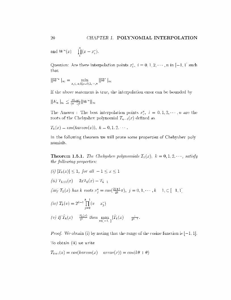
Question: Are there interpolation points x�i ; i = 0; 1; 2; � � � ; n in [�1; 1] suchthat

jjW �jj1 = minxi2[a;b];i=0;1;�� ;n

jjW jj1

If the above statement is true, the interpolation error can be bounded by

jjEnjj1 � Mn+1

(n+1)!jjW �jj1

The Answer : The best interpolation points x�i ; i = 0; 1; 2; � � � ; n are theroots of the Chebyshev polynomial Tn+1(x) de�ned as

Tk(x) = cos(karcos(x)); k = 0; 1; 2; � � � :In the following theorem we will prove some properties of Chebyshev poly-nomials.

Theorem 1.5.1. The Chebyshev polynomials Tk(x); k = 0; 1; 2; � � � , satisfythe following properties:

(i) jTk(x)j � 1; for all � 1 � x � 1

(ii) Tk+1(x) = 2xTk(x)� Tk�1

(iii) Tk(x) has k roots x�j = cos(2j+12k

�); j = 0; 1; � � � ; k � 1;2 [�1; 1]

(iv) Tk(x) = 2k�1k�1Qj=0

(x� x�j)

(v) If ~Tk(x) =Tk(x)2k�1 then max

x2[�1;1]j ~Tk(x)j = 1

2k�1 .

Proof. We obtain (i) by noting that the range of the cosine function is [�1; 1].To obtain (ii) we write

Tk+1(x) = cos(karcos(x) + arcos(x)) = cos(k� + �)


where � = arcos(x) and write

Tk+1 = cos(k� + �)

Tk�1 = cos(k� � �)

Use the trigonometric identity cos(a � b) = cos(a)cos(b) � sin(a)sin(b) toobtain

cos(k� + �) = cos(k�)cos(�)� sin(k�)sin(�)

andcos(k� � �) = cos(k�)cos(�) + sin(k�)sin(�)

Adding the previous equations to obtain

Tk+1(x) + Tk�1(x) = 2cos(k�)cos(�) = 2xTk(x)

This proves (ii).

To obtain the roots we set cos(karcos(x)) = 0 which leads to

karcos(x) =(2j + 1)

2�; j = 0;�1;�2; � � � :

If we solve for x, we obtain

x = cos((2j + 1)

2k�); j = 0;�1;�2; � � � ;

leads to the roots

x�j = cos((2j + 1)

2k�); j = 0; 1; � � � ; k � 1:

Use induction to prove (iv) step 1: T1(x) = 20x, T2(x) = 21x2� 1 (iv) is truefor k = 1; 2.

Step 2: Assume Tk = 2k�1xk +k�1Pi=0

cixi , for k = 1; 2; � � � ; n and use (ii) we

write

Tn+1(x) = 2xTn � Tn�1(x) = 2nxn+1 +nXi=0

aixi


This establishes (iv), i.e., Tk = 2k�1k�1Qj=0

(x� x�j).

Applying (iv) we show that (v) is true.

Corollary 2. If ~Tn(x) is the monic Chebyshev polynomial of degree n, then

max�1�x�1

j ~Qn(x)j � max�1�x�1

j ~Tn(x)j = 1

2n�1; 8 ~Qn 2 ~Pn:

Proof. Assume there is another monic polynomial ~Rn(x) such that

max�1�x�1

j ~Rn(x)j < 1

2n�1

We also note that

~Tn(zk) =(�1)k2n�1

; zk = cos(k�=n); k = 0; 1; 2; � � � ; n:

The (n� 1)-degree polynomial dn�1(x) = ~Tn(x)� ~Rn(x) satis�es

dn�1(z0) > 0, dn�1(z1) < 0, dn�1(z2) > 0, dn�1(z3) < 0 So dn�1(x) changessign between each pair zk and zk+1; k = 0; 1; 2; � � � ; n and thus has n roots.Thus dn�1(x) = 0, identically, i.e., ~T (x) and ~Rn(x) are identical. This leadsto a contradiction with the assumption above.

Below are the �rst �ve Chebyshev polynomials.

T0(x) = 1T1(x) = xT2(x) = 2x2 � 1T3(x) = 4x3 � 3xT4(x) = 8x4 � 8x2 + 1

Example of Chebyshev points:


k x�0 x�1 x�2 x�3

1 0

2p2=2 �p2=2

3p3=2 0 �p3=2

4 cos(�=8) cos(3�=8) cos(5�=8) cos(7�=8)

Application to interpolation:

Let pn(x) 2 Pn interpolate f(x) 2 Cn+1[�1; 1] at the roots of Tn+1(x),x�j ; j = 0; 1; 2; � � � ; n. Thus, we can write the interpolation error formulaas

f(x)� pn(x) =fn+1(�(x))

(n + 1)!~Tn+1(x)

Using (v) from the previous theorem and assuming jjfn+1jj1;[�1;1] � Mn+1

we obtain

maxx2[�1;1]


2n(n + 1)!

Remarks:

1. We note that this choice of interpolation points reduces the error signi�-cantly.

2. With Chebyshev points, pn converges uniformly to f when f 2 C1[�1; 1]only. The function f does not have to be analytic (see Gautschi).

Example 1:

Consider f(x) = ex; x 2 [�1; 1]

Case 1: with three points; n=2:

jjE2jj1 � M3

3!22= e=24 = 0:1136:

Case 2: with 6 points; n=5:


jjE5jj1 � M6

6!25= e=(720� 32) = 0:11710�3:

How many Chebyshev points are needed to have jjEnjj1 < 10�8

jjEnjj1 � Mn+1

2n(n + 1)!=

e

(n+ 1)!2n= 0:13110�9; for n=9:

Thus, 10 Chebyshev points are needed.

Chebyshev points on [a; b]:

Chebyshev points can be used on an arbitrary interval [a; b] using the lineartransformation

x =a+ b

2+b� a

2t; �1 � t � 1: (1.1.2a)

We also need the inverse mapping

t = 2x� a

b� a� 1; a � x � b: (1.1.2b)

First, we order the Chebyshev nodes in [�1; 1] as

t�k = cos(2k + 1

2n+ 2� � �) = �cos(2k + 1

2n+ 2�); k = 0; 1; 2; � � � ; n:

we de�ne the interpolation nodes on an arbitrary interval [a; b] as

x�k =a+ b

2+b� a

2t�k; k = 0; 1; 2; � � � ; n

Remarks:

1. x�0 < x�1 < � � � < x�n

2. x�k are symmetric with respect to the center (a+ b)=2

3. x�k are independent of the interpolated function f


Theorem 1.5.2. Let f 2 Cn+1[a; b] and pn interpolate f at the Chebyshevnodes x�k; k = 0; 1; 2; � � � ; n, in [a,b]. Then

maxx2[a;b]

jf(x)� pn(x)j � 2Mn+1(b� a)n+1

4n+1(n+ 1)!:

Where Mn+1 = maxx2[a;b]

jf (n+1)(x)j .

Proof. It suÆces to rewrite W (x) =nQi=0

(x � xi�) using the mapping (1.1.2)

to �nd that

(x� x�i ) =b� a

2(t� t�i );

and

W (x) =nYi=0

(x� xi�) = (b� a

2)n+1

nYi=0

(t� t�i ) = (b� a

2)n+1 ~Tn+1(t):

Finally, using jj ~Tn+1jj1;[�1;1] =12n

we complete proof.

Example 2:

Consider f(x) = 3x = eln(3)x; x 2 [0; 1] whose derivative is f (n+1)(x) =ln(3)n+1eln(3)x. Noting that f (n+1) is a monotonically increasing function,Mn+1 = f (n+1)(1) = 3ln(3)n+1. Therefore,

jjEnjj1 � 2� 3 ln(3)n+1

4n+1(n+ 1)!=

6 ln(3)n+1

4n+1(n + 1)!:


# of Chebyshev points Error bound2 0.2263 0.02074 0.001425 0.0000786 0.358 10�5

7 0.140 10�6

8 0.48 10�8

9 0.14 10�9

1.6 Hermite interpolation

We restate the general Hermite interpolation by Letting x0 < x1 < x2 � � �xmbe m+ 1 distinct points such that

f (k)(xi) = p(k)n (xi); k = 0; 1; � � �ni � 1; i = 0; 1; � � �m; (1.1.3)

wheremPi=0

ni = n+ 1 and ni � 1. We note that ni =1; i = 0; � � � ; m; leads toLagrange interpolation.

1.6.1 Lagrange form of Hermite interpolation polyno-

mials

Theorem 1.6.1. There exists a unique polynomial pn(x) that satis�es (1.1.3)with ni = 2 and n = 2m + 1.

Proof. Existence:

Next, we study the special case ni = 2; i = 0; 1; 2; � � � ; where

li;1(x) = (x� xi)li(x)2: (1.1.4)

1.6. HERMITE INTERPOLATION 27

and

li;0 = li(x)2 � 2l0i(xi)(x� xi)li(x)

2: (1.1.5)

Now, we can verify that

li;1(xj) = 0; j = 0; 1; 2; � � � ; m

l0i;1(x) = 2(x� xi)l0i(x)li(x) + li(x)

2:

Thus, l0i;1(xj) = Æij.

One can easily check that li;0(xj) = Æij.

For l0i;0(x) we have

l0i;0(x) = (1� 2l0i(xi)(x� xi))2l0i(x)li(x)� 2l0i(xi)li(x)

2:

Thus, l0i;0(xj) = 0; j = 0; 1; � � � ; m:Existence of Hermite interpolation polynomial is established by writing theLagrange form of Hermite polynomial as

pn(x) =mXi=0

f(xi)li;0(x) +mXi=0

f 0(xi)li;1(x): (1.1.6)

Uniqueness:

Assume there are two polynomials pn(x) and qn(x) that satisfy (1.1.3) andconsider the di�erence dn(x) = pn(x)� qn(x) which satis�es

d(s)n (xj) = 0; s = 0; 1; j = 0; 1; � � � ; m:

Thus, dn(x) is a polynomial of degree at most n and has (n+1) roots countingthe multiplicity of each root. The fundamental theorem of Algebra showsthat dn(x) is identically zero. With this we establish the uniqueness of pnand �nish the proof of the theorem.


1.6.2 Newton form of Hermite interpolation polyno-

mial

Using the following relation

f [x0; x0 + h; x0 + 2h; � � � ; x0 + kh] =f (k)(�)

k!; x0 < � < x0 + kh (1.1.7)

and taking the limit when h! 0 we obtain that

f [x0; x0; x0; � � � ; x0] = fk(x0)

k!: (1.1.8)

The divided di�erence table for the data (xk+ ih; f(x0+kh)); i = 0; 1; 2; 3; 4will converge to the table shown below where we recover the Taylor polyno-mial about xk and with nk = 5.

Using this observation we initialize the table for xk and nk = 5 as follows:

(i) every point xi is repeated ni times

(ii) we set zi = xk; zi+1 = xk; � � � ; zi+4 = xk

(iii) we initialize f [zi; zi+1; � � � ; zi+s] =f(s)(xk)

s!as shown in the following table

zi xk f(xk)zi+1 xk f(xk) f 0(xk)zi+2 xk f(xk) f 0(xk) f 00(xk)=2!zi+3 xk f(xk) f 0(xk) f 00(xk)=2! f

000

(xk)=3!zi+4 xk f(xk) f 0(xk) f 00(xk)=2! f

000

(xk)=3! f (4)(xk)=4!

The general formula for divided di�erences with repeated arguments for x0 �x1 � : : : < xn is given by

f [xi; xi+1; : : : ; xi+k] =

(f [xi+1;xi+2;::: ;xi+k]�f [xi;::: ;xk�1]

xi+k�xi; if xi 6= xi+k

f(k)(�)k!

Example: Let f(x) = x4 + 1, f 0(x) = 4x3. We will construct a polynomialp5(x) such that p(xi) = f(xi) and p0(xi) = f 0(xi) with xi = �1; 0; 1. TheHermite divided di�erence table is given as


zi f(zi) 1 DD 2 DD 3 DD 4 DD 5 DDz0 -1 2

z1 -1 2 f 0(�1) = �4z2 0 1 -1 3

z3 0 1 f 0(0) = 0 1 -2

z4 1 2 1 1 0 1

z5 1 2 f 0(1) = 4 3 2 1 0

The forward Hermite polynomial is given as

p5(x) = 2� 4(x + 1) + 3(x + 1)2 � 2(x+ 1)2x + (x+ 1)2x2 = 1 + x4

(1.1.9)

The Hermite polynomial that interpolates f and f 0 at x = �1; 0 is given as

p3(x) = 2� 4(x+ 1) + 3(x+ 1)2 � 2(x + 1)2x: (1.1.10)

The backward Hermite polynomial is given as

p5(x) = 2� 4(x� 1) + 3(x� 1)2 + 2(x� 1)2x + (x� 1)2x2 = 1 + x4

(1.1.11)

The Hermite polynomial that interpolates f and f 0 at x = 0; 1 is given by

p3(x) = 2 + 4(x� 1) + 3(x� 1)2 + 2(x� 1)2x: (1.1.12)

Example:

Consider the data with m = 1; n0 = 1; n1 = 2 given in the following table

xi 0 1f(xi) 1 2f 0(xi) 0 1f 00(xi) NA 2

We write the divided di�erences table as


zI f(zi) 1DD 2DD 3 DD 4DDz0 0 1

z1 0 1 f 0(x0) = 0

z2 1 2 1 1

z3 1 2 f 0(x1) = 1 0 -1

z4 1 2 f 0(x1) = 1 f 00(x1)=2! = 1 1 2

The Hermite polynomial is given as

H4(x) = 1 + 0(x� 0) + (x� 0)2 � (x� 0)2(x� 1) + 2(x� 0)2(x� 1)2

= 1 + 2x2 � x3 + 2x2(x� 1)2: (1.1.13)

1.6.3 Hermite interpolation error

Theorem 1.6.2. Let f(x) 2 C[a; b] be 2m + 2 di�erentiable on (a; b) andconsider x0 < x1 < x2; � � � ; xm in [a; b] with ni = 2; i = 0; 1; � � � ; m. If p2m+1

is the Hermite polynomial such that p(k)2m+1(xi) = f (k)(xi), i = 0; 1; � � � ; m,k = 0; 1, then there exists �(x) 2 [a; b] such that

f(x)� p2m+1(x) =f (2m+2)(�(x))

(2m+ 2)!W (x) (1.1.14a)

where

W (x) =mYi=0

(x� xi)2: (1.1.14b)

Proof. We consider the special case ni = 2; i.e., n = 2m + 1, select anarbitrary point x 2 [a; b]; x 6= xi; i = 0; � � � ; m and de�ne the function

g(t) = f(t)� p2m+1(t)� f(x)� p2m+1(x)

W (x)W (t): (1.1.15)


We note that g has (m+2) roots, i.e., g(xi) = 0; i = 0; 1; � � �m and g(x) = 0.Applying the generalized Rolle's Theorem we show that

g0(�i) = 0; i = 0; 1; � � � ; m where �i 2 [a; b], �i 6= xj, �i 6= x.

Using (1.1.3) with ni = 2 we have g0(xi) = 0; i = 0; 1; � � � ; m. Thus, g0(t)has 2m+ 2 roots in [a; b].

Applying the generalized Rolle's theorem we show that there exists � 2 (a; b)such that

g(2m+2)(�) = 0:

Combining this with (1.1.15) yields

0 = f (2m+2)(�)� f(x)� p2m+1(x)

W (x)(2m + 2)!

Solving for f(x)� p2m+1(x) leads to (1.1.14).

Corollary 3. If f(x) and p2m+1(x) are as in the previous theorem, then

jf(x)� p2m+1(x)j < M2m+2

(2m+ 2)!jW (x)j; x 2 [a; b] (1.1.16)

and

jjf(x)� p2m+1(x)jj1;[a;b] � M2m+2

(2m+ 2)!(b� a)2m+2: (1.1.17)

Proof. The proof is straight forward.

At this point we would like to note that we can prove a uniform convergenceresult under the same conditions as for Lagrange interpolation.

Example: Let f(x) = sin(x); x 2 [0; �=2] and p5(x) interpolate f and f 0 atxi = 0; 0:2; �

2, with ni = 2 and 2m+ 2 = 6


Using the error bound 1.1.16 with M2m+2 = 1, ni = 2 and

W (x) = [(x� 0)(x� 0:2)(x� �

2)]2;

we obtain

jE5(1:1)j � jW (1:1)j6!

� 0:466082

6!� 3:017 10�4: (1.1.18)

1.7 Spline Interpolation

In this section we will study piecewise polynomial interpolation and writethe interpolation errors in terms of the subdivision size and the degree ofpolynomials.

1.7.1 Piecewise Lagrange interpolation

We construct the piecewise linear interpolation for the data (xi; f(xi)); i =0; 1; � � � ; n such that x0 < x1 < � � � < xn as

P1(x) =

8><>:p1;0(x) = f(x0)

(x�x1)x0�x1

+ f(x1)(x�x0)x1�x0

; x 2 [x0; x1];

p1;i(x) = f(xi)(x�xi+1)xi�xi+1

+ f(xi+1)(x�xi)xi+1�xi

; x 2 [xi; xi+1]:

i = 0; 1; � � � ; n� 1:

(1.1.19)

The interpolation error on (xi; xi+1) is bounded as

jjE1;i(x)jj � M2;i

2j(x� xi)(x� xi+1)j; x 2 (xi; xi+1); (1.1.20)

where M2;i = maxxi�x�xi+1

jf (2)(x)j. This can be written as

jjE1;ijj1 � M2;ih2i

8; hi = xi+1 � xi: (1.1.21)

The global error is

1.7. SPLINE INTERPOLATION 33

jjE1jj1 � M2H2

8; H = max

i=0;�� ;n�1hi: (1.1.22)

Theorem 1.7.1. Let f 2 C0[a; b] be twice di�erentiable on (a; b). If P1(x)is the piecewise linear interpolant of f at xi = a + i � h; i = 0; 1; � � � ; n,h = (b� a)=n, then P1 converges uniformly to f as n!1.

Proof. We prove this theorem using the error estimate (1.1.22).

For piecewise quadratic interpolation we select h = (b � a)=n and constructp2;i that interpolates f at xi, (xi + xi+1)=2 and xi+1. In this case the inter-polation error is bounded as

jjE2;ijj1 � M3;i(hi=2)3

9p3

; hi = xi+1 � xi: (1.1.23)

A global bound is

jjE2jj1 � M3(H=2)3

9p3

; H = maxi=0;�� ;2n�1

hi: (1.1.24)

Theorem 1.7.2. Let f 2 C0[a; b] and be m+1 times di�erentiable on (a; b)and x0 < x1 < � � � < xn with hi = xi+1 � xi and H = max

ihi. If Pm(x) is

the piecewise polynomial of degree m on each subinterval [xi; xi+1] and Pm(x)interpolates f on [xi; xi+1] at xi;k = xi + k � ~hi; k = 0; 1; � � � ; m, ~hi = hi=m,then Pm converges uniformly to f as H ! 0.

Proof. Again we prove this theorem using the error bound

jjEmjj1 � Mm+1Hm+1

(m+ 1)!; H = max

i=0;1;�� ;nm�1hi: (1.1.25)

Similarly, we may construct piecewise Hermite interpolation polynomials fol-lowing the same line of reasoning as for Lagrange interpolation.


1.7.2 Cubic spline interpolation

We use piecewise polynomials of degree three that are C2 and interpolate thedata such as S(xk) = f(xk) = yk; k = 0; 1; � � �n.

Algorithm

(i) Order the points xk; x = 0; 1; � � �n such that

a = x0 < x1 < x2 < � � �xn�1 < xn = b:

(ii) Let S(x) be a piecewise spline de�ned by n cubic polynomials such that

S(x) = Sk(x) = ak + bk(x� xk) + ck(x� xk)2 + dk(x� xk)

3; xk � x � xk+1

(iii) �nd ak; bk; ck; dk; k = 0; 1; � � �n� 1 such that

(1) S(xk) = yk; k = 0; 1; � � � ; n(2) Sk(xk+1) = Sk+1(xk+1); k = 0; � � � ; n� 2

(3) S0

k(xk+1) = S0

k+1(xk+1); k = 0; � � � ; n� 2

(4) S00

k (xk+1) = S00

k+1(xk+1); k = 0; � � � ; n� 2

Theorem 1.7.3. If A is an n� n strictly diagonally dominant matrix, i.e.,

jakkj >nP

i=1;i6=k

jak;ij; k = 1; 2; � � �n, then A is nonsingular.

Proof. By contradiction, we assume that A is singular, i.e., there exists anonzero vector x such that Ax = 0 and let xk such that jxkj = maxjxij.This leads to

akkxk = �nX

i=1;i6=k

akixi: (1.1.26)

Taking the absolute value and using the triangle inequality we obtain

jakkjjxkj �nX

i=1;i6=k

jakijjxij: (1.1.27)


Dividing both terms by jxkj we get

jakkj �nX

i=1;i6=k

jakij jxijjxkj �nX

i=1;i6=k

jakij (1.1.28)

This leads to a contradiction since A is strictly diagonally dominant.

Theorem 1.7.4. Let us consider the set of data points (xi; f(xi)); i =0; 1; � � � ; n; such that x0 < x1 < � � � ; xn. If S 00(x0) = S 00(xn) = 0, thenthere exists a unique piecewise cubic polynomial that satis�es the conditions(iii).

Proof. Existence: we assume S"(xk) = mk where hk = xk+1 � xk and usepiecewise linear interpolation of S" to write

S00

k (x) = mkx� xk+1

xk � xk+1

+mk+1x� xk

xk+1 � xk

= �mk

hk(x� xk+1) +

mk+1

hk(x� xk); xk � x � xk+1

With this de�nition of S", condition (4) is automatically satis�ed.

Integrating S00

k (x) we obtain

Sk(x) = �mk

6hk(x� xk+1)

3 +mk+1

6hk(x� xk)

3 + pk(xk+1 � x) + qk(x� xk)

Need to �nd mk; qk and pk; k = 0; 1; 2; � � � ; n� 1:

In order to enforce the conditions (1) and (2) we write

Sk(xk) = yk =mk

6h2k + pkhk

Sk(xk+1) = yk+1 =mk+1

6h2k + qkhk

Solve for pk and qk to solve

pk =ykhk� mkhk

6(1.1.29a)


qk =yk+1

hk� mk+1hk

6: (1.1.29b)

We note that if mk; k = 0; 1; : : : ; n are known, The previous equations maybe used to compute pk and qk.

Now, substitute pk and qk in the equation for Sk to have

Sk(x) = �mk

6hk(x� xk+1)

3 +mk+1

6hk(x� xk)

3 + (ykhk� mkhk

6)(xk+1 � x)+

(yk+1

hk� mk+1hk

6)(x� xk) (1.1.30)

Applying condition (3) to enforce the continuity of S0

(x)

S0

k(xk+1) = S0

k+1(xk+1); k = 0; 1; � � � ; n� 1: (1.1.31)

where

S 0k(x) = �mk

2hk(x� xk+1)

2 +mk+1

2hk(x� xk)

2 �

(ykhk� mkhk

6) + (

yk+1

hk� mk+1hk

6); xk � x � xk+1; (1.1.32)

and

S 0k+1(x) = �mk+1

2hk+1(x� xk+2)

2 +mk+2

2hk+1(x� xk+1)

2 �

(yk+1

hk+1� mk+1hk+1

6) + (

yk+2

hk+1� mk+2hk+1

6); xk+1 � x � xk+2: (1.1.33)

Taking the limit from the left at xk+1 leads to

S0

k(xk+1) =mk+1hk

3+mkhk6

+ dk: (1.1.34)

Taking the limit from the right at xk+1 yields


S0

k+1(xk+1) = �mk+1hk+1

3� mk+2hk+1

6+ dk+1

where

dk =yk+1 � yk

hk; k = 0; 1; � � � ; n� 1

Using (1.1.31) we obtain the following system having n + 1 unknowns andn� 1 equations.

(I)

(mkhk + 2mk+1(hk + hk+1) +mk+2hk+1 = 6(dk+1 � dk);

k = 0; 1; 2; � � � ; n� 2:(1.1.35)

Now we need to close the system by adding two more equations from S 00(x0) =0 and S 00(xn) = 0 which leads to

m0 = 0; mn = 0: (1.1.36)

This is called the natural spline.

The system (1.1.35) and (1.1.36) lead to

(I:NAT )

8><>:(2h0 + 2h1)m1 + h1m2 = u0

mkhk + 2mk+1(hk + hk+1) +mk+1hk+1 = uk; 1 � k � n� 3

hn�2mn�2 + 2(hn�2 + hn�1)mn�1 = un�2

In matrix form we write2666664

2(h0 + h1) h1 0 � � � 0

h1 2(h1 + h2) h2. . . 0

0 h2 2(h2 + h3) � � � 0...

. . . . . . . . . hn�2

0 � � � 0 hn�2 2(hn�2 + hn�1)

3777775

2666664

m1

m2

m3...

mn�1

3777775=

2666664

u0u1u2...

un�2

3777775

The resulting matrix is strictly symmetric positive de�nite and diagonallydominant and yields a unique solution.


Other splines include:

Not-a-Knot Spline:

We add the following two conditions:

S000

0 (x1) = S000

1 (x1) which leads to

m1 �m0

h0=m2 �m1

h1(1.1.37)

and the condition

S000

n�2(xn�1) = S000

n�1(xn�1) which leads to

mn �mn�1

hn�1=mn�1 �mn�2

hn�2(1.1.38)

Solve (1.1.37) and (1.1.38) for m0 and mn to obtain

m0 = (1 + h0=h1)m1 � (h0=h1)m2 (1.1.39)

mn = �hn=hn1mn�2 + (1 + hn=hn�1)mn�1 (1.1.40)

Substitute into the system (1.1.35) to obtain

(I:NK)

8><>:(3h0 + 2h1 + h20=h1)m1 + (h1 � h20=h1)m2 = u0

mkhk + 2mk+1(hk + hk+1) +mk+1hk+1 = uk; k = 1; � � � ; n� 3

(hn�2 � h2n�1=hn�2)mn�2 + (2hn�2 + 3hn�1 + h2n�1=hn�2)mn�1 = un�2

where uk = 6(dk+1 � dk); k = 0; 1; � � � ; n � 2. We solve the system form1; m2; � � �mn�1 and use (1.1.39) and (1.1.40) to �nd m0 and mn.

Use (1.1.29) to �nd pk and qk; k = 0; 1; � � �n� 1. Finally, we use the formula(1.1.30) that de�nes Sk(x).


Clamped Spline:

We close the system (I) using the following conditions

S0

0(x0) = f0

(x0)

S0

n�1(xn) = f0

(xn)

S 00(x) = �m0

2h0(x� x1)

2 +m1

2h0(x� x0)

2 � (y0h0� m0h0

6) + (

y1h0� m1h0

6)

S 00(x0) = �m0h03

� m1h06

+y1 � y0h0

:

The boundary equation S 00(x0) = f 0(x0) leads to

2m0h0 +m1h0 = 6(d0 � f 0(x0)) (1.1.41)

The boundary condition S 0n�1(xn) = f 0(xn) yields the equation

S 0n�1(xn) =mnhn�1

3+mn�1hn�1

6+ dn�1 = f 0(xn);

which leads

2mnhn�1 +mn�1hn�1 = 6(f 0(xn)� dn�1) (1.1.42)

Now, the system (I) is reduced to

(I:CL)

8><>:(3h0

2+ 2h1)m1 + h1m2 = u0 � 3(d0 � f 0(x0))

mkhk + 2mk+1(hk + hk+1) +mk+1hk+1 = uk; k = 1; 2; � � � ; n� 3

hn�2mn�2 + (2hn�2 +3hn�1

2)mn�1 = un�2 � 3(f 0(xn)� dn�1)

Matrix formulation for the not-a-knot spline

AM = U


where

A =

266666664

3h0 + 2h1 +h20h1

h1 � h20h1

0 � � � 0

h1 2(h1 + h2) h2. . . 0

0 h2 2(h2 + h3) � � � 0...

. . . . . . . . . hn�2

0 � � � 0 hn�2 � h2n�1

hn�22hn�2 + 3hn�1 +

h2n�1

hn�2

377777775

M =

2666664

m1

m2

m3...

mn�1

3777775 ; B =

2666664

u0u1u2...

un�2

3777775

The system admits a unique solution since the matrix is strictly diagonallydominant.

Example 1: consider the function f(x) = x=(2 + x) at �1; 1; 2; 3

xi f(xi) 1stDD 6*(2nd Di�)�1 �1

2=31 1=3 �3

1=62 1=2 �2=5

1=103 3=5

h0 = 2, h1 = 1, h2 = 1.

�3h0 + 2h1 + h20=h1 h1 � h20=h1

h1 � h22=h1 2h1 + 3h2 + h22=h1)

� �m1

m2

�=

�u0u1

��12 �30 6

� �m1

m2

�=

� �3�2=5

�

The solution is m1 = �4=15, m2 = �1=15


Matrix formulation for the clamped spline

2666664

(3h02+ 2h1) h1 0 � � � 0

h1 2(h1 + h2) h2. . . 0

0 h2 2(h2 + h3) � � � 0...

. . . . . . . . . hn�2

0 � � � 0 hn�2 (2hn�2 +3hn�1

2)

3777775

2666664

m1

m2

m3...

mn�1

3777775

=

2666664

u0 � 3(d0 � f 0(x0))u1u2...

un�2 � 3(f 0(xn)� dn�1)

3777775

The system admits a unique solution since the matrix is symmetric diagonallydominant and positive de�nite (SPD).

Example 1:

Let us interpolate the function f(x) = x=(2 + x) where f 0(x) = 2=(2 + x)2.Thus S 00(x0) = 2 = f 0(�1) and S 0n�1(x3) = 2=25 = f 0(3).

To compute the ui; i = 0; 1 we use the following table


2=31 1=3 �3

1=62 1=2 �2=5

1=103 3=5

h0 = 2, h1 = 1, h2 = 1.�3h0=2 + 2h1 h1

h1 2h1 + 3h2=2)

� �m1

m2

�=

�u0 � 3(d0 � f 0(x0))u1 � 3(f 0(x3)� d2)

�


�5 11 7=2

� �m1

m2

�=

�1

�17=50�

The solution is m1 = 64=275, m2 = �9=55

m0 = 3f [x0;x1]�f 0(x0)h0

�m1=2 = �582=275

m3 = 3f 0(x3)�f [x2;x3]h2

�m2=2 = 6=275

On [-1,1] :

p0 = y0=h0 � (m0h0)=6 = 113=550, q0 = y1=h0 � (m1h0)=6 = 49=550

S0(x) =582

12� 275(x� 1)3 +

64

12� 275(x + 1)3

+113

550(1� x) +

49

550(x+ 1)

On [1; 2]

p1 = y1=h1 � (m1h1)=6 = 81=275,

q1 = y2=h1 � (m2h1)=6 = 29=55

S1(x) = � 64

6� 275(x� 2)3 � 9

6� 55(x� 1)3

+81(2� x)=275 + 29(x� 1)=55

On [2,3]

p2 = y2=h2 � (m2h2)=6 = 29=55, q2 = y3=h2 � (m3h2)=6 = 164=275

S2(x) =9

6� 55(x� 3)3 � 1

275(x� 2)3

+29(3� x)=55 + 164(x� 2)=275

Examples of natural spline approximations


Example 1: Let f(x) = jxj and construct the cubic spline interpolation atthe points xi = �2 + i; i = 0; 1; 2; 3; 4

xi f(xi) 1stDD 6*(2nd Di�)�2 2

�1�1 1 0

�10 0 12

11 1 0

12 2

We note that hi = h; i = 0; 1; 2; 3, m0 = m4 = 0 which leads to the followingsystem

244 1 01 4 10 1 4

3524m1

m2

m3

35 =

24 0120

35

The solution is m1 = �6=7, m2 = 24=7, m3 = �6=7.

On [�2;�1]

p0 = (y0 � m0h206

)=h0 = (2� 0)=1 = 2 q0 = (y1 � m1h206

)=h0 = (1 + 1=7) = 8=7

S0(x) = �1

7(x+ 2)3 + 2(�1� x) +

8

7(x + 2)

On [�1; 0]

p1 = (y1 � m1h216

)=h1 = (2� 0)=1 = 8=7

q1 = (y2 � m2h216

)=h1 = (1 + 1=7) = �4=7

S1(x) =1

7x3 +

4

7(x+ 1)3 +

8

7(0� x)� 4

7(x+ 1)


On [0; 1]

p2 = (y2 � m2h226

)=h2 = (0� 247�6

) = �4=7

q2 = (y3 � m3h226

)=h2 = (1 + 16�7

) = 8=7

S2(x) = �4

7(x� 1)3 � x3=7� 4

7(1� x) +

8

7x

On [1; 2]

p3 = (y3 � m3h236

)=h3 = 8=7, q3 = (y4 � m4h236

)=h3 = 2

S3(x) = �(2� x)3=7 + 2(x� 1) + 8(2� x)=7

p = (2; 8=7;�4=7; 8=7), q = (8=7;�4=7; 8=7; 2)

Example 2:


2=31 1=3 �3

1=62 1=2 �2=5

1=103 3=5

h0 = 2, h1 = 1, h2 = 1.

Natural cubic spline leads to m0 = m3 = 0. The other coeÆcients satisfy thesystem

�2(h0 + h1) h1

h1 2(h1 + h2)

� �m1

m2

�=

� �3�2=5

��6 11 4

� �m1

m2

�=

� �3�2=5

�


which admits the following solution m1 = � 58115

, m2 =3

115

On [�1; 1]

p0 = (y0 � m0h206

)=h0 = �1=2, q0 = (y1 � m1h206

)=h0 = 77=230

On [1; 2]

p1 = (y1 � m1h216

)=h1 = 48=115, q1 = (y2 � m2h216

)=h1 = 57=115

On [2; 3]

p2 = (y2 � m2h226

)=h2 = 57=115, q2 = (y3 � m3h226

)=h2 = 3=5

p = [�1=2; 48=115; 57=115], q = [77=230; 57=115; 3=5]

Matlab commands for splines

x=0:1:10;

y=sin(x);

xi=0:0.2:10;

yi = sin(xi);

%piecewise linear interpolation

y1 = interp1(x,y,xi)

plot(x,y,'0',xi,yi) %plot the exact function

hold on;

plot(xi,y1);

%

y2 = interp1(x,y,xi,'spline') % spline interpolation

y3 = interp1(x,y,'cubic') % piecewise cubic interpolation

y4 = spline(x,y,xi) %not-a-knot spline

plot(xi,y4);

plot(xi,y2);

plot(xi,y3);


1.7.3 Convergence of cubic splines

We will study the uniform convergence of the clamped cubic spline for f 2C4[a; b].We �rst write the matrix formulation for the clamped cubic spline as

AM = B

where M = [m0; m1; � � � ; mn]t, B = [b0; b1; � � � ; bn]t.

Let us recall that

S 00(x0) =h0m0

3+h0m1

6=

(y1 � y0)

h0� f 0(x0)

and

S 0n�1(xn) =hn�1mn�1

6+hn�1mn

3= f 0(xn)� (yn � yn�1)

hn�1:

We combine (1.1.41), (1.1.42) and (1.1.35) to write the (n + 1) � (n + 1)matrix A as

ai;j =

8>>>>>><>>>>>>:

2; if i = j

1; if (i; j) = (1; 2) or (i; j) = (n; n� 1)hi

hi+hi�1; if j = i+ 1; 1 < i < n

hi�1

hi+hi�1; if j = i� 1; 1 � i < n� 1

0; otherwise;

: (1.1.43)

the n+ 1 by n+ 1 matrix A can be written as

A =

26666664

2 1 0 0 : : : 0. . . . . .

.... . . hi�1

hi+hi�12 hi

hi+hi�1: : : 0

. . . . . ....

0 0 0 : : : 1 2

37777775

(1.1.44)

The right-hand side B is de�ned by

b0 =6

h0(y1 � y0h0

� f 0(x0)); (1.1.45)


bi =6

hi + hi�1

(yi+1 � yi

hi� yi � yi�1

hi�1

); i = 1; 2; � � � ; n� 1; (1.1.46)

bn =6

hn�1(f 0(xn)� yn � yn�1

hn�1): (1.1.47)

Lemma 1.7.1. Let A be de�ned in (1.1.43) such that Az = w. Then,

jjzjj1 � jjwjj1Proof. Let zk be such that jzkj = jjzjj1. The kth equation from Az = w

leads to

ak;k�1zk�1 + 2zk + ak;k+1zk+1 = wk (1.1.48)

Applying the triangle inequality we have

jjwjj1 � jwkj = jak;k�1zk�1 + 2zk + ak;k+1zk+1j (1.1.49)

� 2jzkj � ak;k�1jzk�1j � ak;k+1jzk+1j (1.1.50)

� (2� (ak;k�1 + ak;k+1)jzkj: (1.1.51)

Using the fact that ak;k�1 + ak;k+1 = 1 we complete the proof.

In order to state the following lemma we let F = [f 00(x0); f00(x1); � � � ; f 00(xn)]t,

R = B�AF = A(M� F) and H = maxi=0;��n�1

hi.

Lemma 1.7.2. If f 2 C4[a; b] and jjf (4)jj1 �M4, then

jjM� Fjj1 � jjRjj1 � 3

4M4H

2: (1.1.52)


Proof.

r0 = b0 � 2f 00(x0)� f 00(x1) =6

h0(y1 � y0h0

� f 0(x0))� 2f 00(x0)� f 00(x1):

(1.1.53)

Using Taylor expansion we write

y1 � y0h0

=f(x0 + h0)� f(x0)

h0(1.1.54)

=1

h0(h0f

0(x0) +h20f

00(x0)

2+h30f

000(x0)

6+h40f

(4)(�1)

24) (1.1.55)

f 00(x0 + h0) = f 00(x0) + h0f000(x0) +

h20f(4)(�2)

2(1.1.56)

which leads to

r0 =h20f

(4)(�1)

4� h20f

(4)(�2)

2(1.1.57)

Thus,

jr0j < 3H2M4=4: (1.1.58)

Similarly for

rn = bn � f 00(xn�1)� 2f 00(xn): (1.1.59)

bn =6

hn�1(f 0(xn)� yn � yn�1

hn�1) (1.1.60)

Using Taylor series

f(xn)� f(xn�1)

hn�1

= �f(xn�1)� f(xn)

hn�1

=

�1hn�1

(�hn�1f0(xn) +

h2n�1

2f 00(xn)� h3n�1

6f 000(xn) +

h4n�1

24f (4)(�1)): (1.1.61)


f 00(xn�1) = f 00(xn � hn�1) = f 00(xn)� hn�1

2f 000(xn) +

h2n�1

2f (4)(�2) (1.1.62)

jrnj < 3H2M4=4: (1.1.63)

rj = bj � �jf00(xj�1)� 2f 00(xj)� �jf

00(xj+1); (1.1.64a)

where

�j =hj�1

hj + hj�1

; �j =hj

hj + hj�1

(1.1.64b)

and

bj =6

hj�1 + hj(yj+1 � yj

hj� yj � yj�1

hj�1): (1.1.64c)

Using Taylor expansion we write

yj+1 � yjhj

= [f 0(xj) +hjf

00(xj)

2+h2jf

000(xj)

6+h3jf

(4)(�1)

24]; (1.1.64d)

yj � yj�1

hj�1= [+f 0(xj)� hj�1f

00(xj)

2+h2j�1f

000(xj)

6� h3j�1f

(4)(�2)

24];

(1.1.64e)

f 00(xj�1) = f 00(xj)� hj�1f000(xj) + h2j�1f

(4)(�3)=2; (1.1.64f)

f 00(xj+1) = f 00(xj) + hjf000(xj) + h2jf

(4)(�4)=2: (1.1.64g)

Note that �i 2 (xj�1; xj+1).

Combining (1.1.64) we obtain

rj =1

hj + hj�1[h3jf

(4)(�1)

4+h3j�1f

(4)(�2)

4� h3j�1f

(4)(�3)

2� h3jf

(4)(�4)

2]:

(1.1.65)


This can be bounded as

jrjj � 3

4M4

h3j + h3j�1

hj + hj�1(1.1.66)

Without loss of generality we assume hj � hj�1 and write

h3j + h3j�1

hj + hj�1= h2j

1 + (hj�1

hj)3

1 +hj�1

hj

� h2j � H2: (1.1.67)

Thus,

jrjj < 3

4M4H

2: (1.1.68)

Finally, using Lemma 1.7.1 we have

jjM� Fjj1 � jjRjj1 � 3

4M4H

2; (1.1.69)

which completes the proof.

Theorem 1.7.5. Le f(x) 2 C4[a; b], a � x0 < x1 < � � � < xn � b, hj =xj+1� xj and H = max

i=0;�� ;n�1hj. Assume there exits K > 0 independent of H

such that

H

hj� K; j = 0; 1; � � � ; n� 1: (1.1.70)

If S(x) is the clamped cubic spline approximation of f at xi; i = 0; 1; � � � ; xn,then there exists Ck > 0 independent of H such that

jjf (k) � S(k)jj1;[a;b] � CkM4KH4�k; k = 0; 1; 2; 3; (1.1.71)

where M4 = jjf (4)jj1.Proof. For k = 3 and x 2 [xj�1�xj ] by adding and subtracting few auxiliaryterms the error can be written

e000(x) = f 000(x)� S 000(x) = f 000(x)� mj �mj�1

hj�1


= f 000(x)� mj � f 00(xj)

hj�1+mj�1 � f 00(xj�1)

hj�1

�f00(xj)� f 00(x)

hj�1+f 00(xj�1)� f 00(x)

hj�1: (1.1.72)

Using Lemma 1.7.2 we bound the following terms

jmj � f 00(xj)

hj�1j � 3M4H

2

4hj�1; jmj�1 � f 00(xj�1)

hj�1j � 3M4H

2

4hj�1: (1.1.73)

We use Taylor series to obtain

f 00(xj)� f 00(x) = (xj � x)f 000(x) +(xj � x)2

2f (4)(�1)

and

f 00(xj�1)� f 00(x) = (xj�1 � x)f 000(x) +(xj�1 � x)2

2f (4)(�2)

we bound the error

je000(x)j � 3M4H2

4hj�1+

1

hj�1j(xj � x)f 000(x) + (xj � x)2f (4)(�1) (1.1.74)

�(xj�1 � x)f 000(x)� (xj�1 � x)2

2f (4)(�2)� hj�1f

000(x)j (1.1.75)

The f 000 terms cancel out to give

je000(x)j � 3M4H2

2hj�1+M4

2hj[(xj � x)2 + (xj�1 � x)2]:

Usingjj(xj � x)2 + (xj�1 � x)2jj1;[xj�1;xj ] = h2j�1 � H2;

we write

je000(x)j � 3M4H2

2hj�1+M4H

2

2hj�1: (1.1.76)

Since H=hj � K we have


jf 000(x)� S 000(x)j � 2M4KH; 8x: (1.1.77)

For k = 2, we note that for each x 2 (a; b), there is xj such that jxj � xj �H=2. Now we rewrite e00(x) as

e00(x) = f 00(x)� S 00(x) = f 00(xj)� S 00(xj) +

Z x

xj

(f 000(t)� S 000(t))dt (1.1.78)

Using j R gj < R jgjdx and Lemma 1.7.2 we obtain

je00(x)j � 3M4H2

4+ j(x� xj)j max

x2[a;b]jjf 000 � S 000jj (1.1.79)

� 3M4H2

4+M4KH2 � 7KM4H

2

4; K > 1: (1.1.80)

Thus,

jjf 00(x)� S 00(x)jj1 � 7KM4H2

4: (1.1.81)

For k = 1, we consider e(t) = f(t)�S(t), since e(xj) = 0, by Rolle's theoremthere exist �j; j = 0; 1; � � � ; n�1 such that e0(�i) = 0 and e0(x0) = e0(xn) = 0.For every x 2 [a; b] there exists �i such that jx � �ij � H and e0(x) can bewritten as

f 0(x)� S 0(x) =

Z x

�i

(f 00(t)� S 00(t))dt (1.1.82)

Thus,

je0(x)j � jx� �ijjje00jj1 � 7

4M4KH3: (1.1.83)


For k = 0, for every x 2 [a; b] there is xj such that jx � xjj � H=2 we alsowrite

f(x)� S(x) =

Z x

xj

(f 0(t)� S 0(t))dt (1.1.84)

je(x)j � jx� xjjjje0jj1 � 7

8M4KH4: (1.1.85)

We conclude that S(k) converges uniformly to f (k) for k = 0; 1; 2; 3 and H !0.

Optimal bounds are proved by Birkho� and De Boor (Burden and Faires) as

jjf � Sjj1 <5

384M4H

4: (1.1.86)

We recall the Hermite interpolation error

jf �H3j < 1

24� 16M4H

4 =M4H

4

384; (1.1.87)

Comparing the cubic spline and Hermite interpolation errors, we see that theratio between the spline and the Hermite errors is only 5. We also note thatHermite interpolation requires the derivative at all the interpolation pointswhile the clamped spline needs the derivatives at the end points only.

Optimality of Splines: The optimality is in the sense that cubic splinehas the smallest curvature. For a curve de�ned by y = f(x) the curvature isde�ned as

� =jf 00(x)jj

[1 + (f 0(x))2]3=2:

Here the curvature is approximated by jf 00(x)j and R b

aS 00(x)2dx is minimized.

More precisely we state the following theorem.


Theorem 1.7.6. If f 2 C2[a; b] and S(x) is the natural cubic spline thatinterpolates f at n+ 1 points xi; i = 0; 1; � � � ; n; thenZ b

a

S 00(x)2dx �Z b

a

f 00(x)2dx: (1.1.88)

Proof. We consider the function e(x) = f(x) � S(x) with e(xi) = 0; i =0; 1; � � � ; n; and write the approximate curvature of f = S + e asZ b

a

f 00(x)2dx =

Z b

a

(S 00(x) + e00(x))2dx =

Z b

a

S 00(x)2dx +

Z b

a

e00(x)2dx+ 2

Z b

a

S 00(x)e00(x)dx: (1.1.89)

We complete the proof by showing that the last term in the right-hand sideof (1.1.89) is 0.

Integrating by parts we obtainZ xi+1

xi

e00(x)S 00(x)dx = S 00(x)e0(x)jx=xi+1x=xi

�Z xi+1

xi

S 000(x)e0(x)dx:

Summing over all intervals, using the fact that e 2 C2 and S 00(a) = S 00(b) = 0.Noting that S 000(x) = Ci is a constant on (xi; xi+1) we obtain

n�1Xi=0

Z xi+1

xi

e00(x)S 00(x)dx = �n�1Xi=0

Ci

Z xi+1

xi

e0(x)dx

= �n�1Xi=0

Ci[e(xi+1)� e(xi)] = 0

We used the fact that e(xi) = 0 we establishR b

aS 00(x)e00(x)dx = 0.

Combining this with (1.1.89) leads to (1.1.88).

The same result holds for the clamped cubic spline with S 0(a) = f 0(a) andS 0(b) = f 0(b). We follow the same line of reasoning to prove it.Thus, among all C2 functions interpolating f at x0; : : : ; xn, the natural cubicspline has the smallest curvature. This includes the clamped spline and not-a=knot splines.


1.7.4 B-splines

We describe a system of B-splines (B stands for basis) from which othersplines can be obtained.

We �rst start with B-splines of degree 0, i.e., piecewise constant splinesde�ned as

B0i (x) =

(1 xi � x < xi+1

0 otherwise; i 2 Z (1.1.90)

Properties of B0i (x):

1. B0i (x) � 0; for all x and i

2.1P

i=�1

B0i (x) = 1, for all x

3. The support of B0i (x) is [xi; xi+1)

4. B0i (x) 2 C�1.

We show property (2) by noting that for arbitrary x there exists m such thatx 2 [xm; xm+1) then write

1Xi=�1

B0i (x) = B0

m(x) = 1:

Use the recurrence formula to generate the next basis functions

Bki (x) =

x� xixi+k � xi

Bk�1i (x) +

xi+k+1 � x

xi+k+1 � xi+1Bk�1

i+1 (x); for k > 0: (1.1.91)

Properties of B1i :

1. B1i (x) are the classical piecewise linear hat functions equal to 1 at xi+1

and zero all other nodes.

2. B1i (x) 2 C0

3.1P

i=�1

B1i (x) = 1 for all x


4. The support of B1i (x) is (xi; xi+2)

5. B1i (x) � 0 for all x and i

In general for arbitrary k one can show that:

1. Bki (x) are piecewise polynomials of degree k

2. Bki (x) 2 Ck�1

3.1P

i=�1

Bki (x) = 1 for all x

4. The support of Bki (x) is (xi; xi+k+1)

5. Bki (x) � 0 for all x and i

6. Bki (x), �1 < i <1 are linearly independent, i.e., they form a basis.

See Figure 1.7.4 for plots of the �rst four b-splines.

Interpolation using B-splines:

(i) For k = 0, we construct a piecewise constant spline interpolation bywriting

f(x) � P0(x) =1X

i=�1

ciB0i (x) (1.1.92)

Using the properties of B0i (x) we show that ci = f(xi).

(ii) For k = 1, we construct a piecewise linear spline interpolation by writing

f(x) � P1(x) =1X

i=�1

ciB1i (x) (1.1.93)

Again using B1i (xj+1) = Æij we show that ci = f(xi+1).

(ii) For k = 3, we construct a piecewise cubic spline interpolation by writing

f(x) � P3(x) =1X

i=�1

ciB3i (x) (1.1.94)


0 2 4 6 80

0.2

0.4

0.6

0.8

1

0 2 4 6 80

0.2

0.4

0.6

0.8

1

0 2 4 6 80

0.2

0.4

0.6

0.8

0 2 4 6 80

0.1

0.2

0.3

0.4

0.5

0.6

0.7

B10(x)

x1 x

2

B11(x)

B12(x)

x1 x

3

x1 x

4

x1 x

5

+ +

+ + +

+ +

+ + +

+ + +

+ +

B13(x)

Figure 1.1: B-splines of degree k = 0; 1; 2; 3, upper left to lower right.


We recall that B3i 2 C2 are piecewise cubic polynomials with support in

(xi; xi+3).

In order to interpolate f at xi; i = 0; � � � ; n, we

1. Write S(x) =n�1Pi=�3

ciB3i (x)

(include basis functions whose support intersect [x0; xn]).

2. Set n+ 1 equations

f(xi) = ci�3B3i�3(xi) + ci�2B

3i�2(xi) + ci�1B

3i�1(xi); i = 0; 1; �; n;

(1.1.95a)

where c�3; c�2; c�1; c0; � � � ; cn are the unknowns.

3. Close the system, for natural Spline, by setting

S 00(x0) = 0; S 00(xn) = 0; (1.1.95b)

4. Solve the system (1.1.95).

Remarks:

1. If xi are uniformly distributed we haveB2

i (xj) = 0; j � i or j � i+ 3,B2

i (xi+1) = B2i (xi+2) = 1=2

B3i (xj) = 0; j � i or j � i+ 4,

B3i (xi+1) = B3

i (xi+3) = 1=6, B3i (xi+2) = 2=3

2. The system (1.1.95) has a unique solution

3. B-splines may be used to construct clamped splines

1.8 Interpolation in multiple dimensions

Read section of 6.10 of textbook (Kincaid and Cheney).

1.9 Least-squares Approximations

Read section 6.8 of Textbook (Kincaid and Cheney).

Bibliography

59

notes - the department of mathematics at virginia tech · notes for numerical analysis math 5466 b...

Documents