notes on stochastic finance - ntu.edu.sg · chapter19 stochasticcalculusforjumpprocesses...

Chapter 19Stochastic Calculus for Jump Processes

In this chapter we present the construction of processes with jumps and inde-pendent increments, including the Poisson and compound Poisson processes.We also with stochastic integrals and stochastic calculus with jumps, andwith the Girsanov Theorem for jump processes, which will be used for pric-ing and the determination of risk-neutral probability measures in the nextchapter, in relation with market incompleteness.

19.1 The Poisson Process . . . . . . . . . . . . . . . . . . . . . . . . . . . 62719.2 Compound Poisson Process . . . . . . . . . . . . . . . . . . . . . 63519.3 Stochastic Integrals with Jumps . . . . . . . . . . . . . . . . . 64019.4 Itô Formula with Jumps . . . . . . . . . . . . . . . . . . . . . . . . 64519.5 Stochastic Differential Equations with Jumps . . . . 65219.6 Girsanov Theorem for Jump Processes . . . . . . . . . . 657Exercises . . . . . . . . . . . . . . . . . . . . . . . . . . . . . . . . . . . . . . . . . . . 664

19.1 The Poisson Process

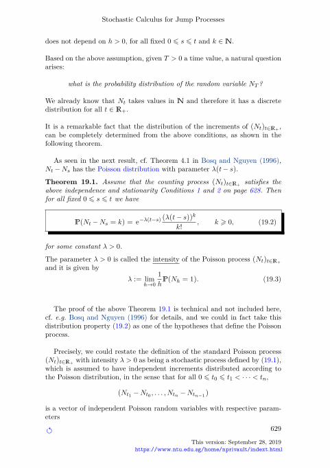
The most elementary and useful jump process is the standard Poisson process(Nt)t∈R+ which is a counting process, i.e. (Nt)t∈R+ has jumps of size +1 only,and its paths are constant in between two jumps.

" 627

This version: September 28, 2019https://www.ntu.edu.sg/home/nprivault/indext.html

https://www.ntu.edu.sg/home/nprivault/indext.html

N. Privault

t

Nt

0

1

2

3

4

5

6

T1 T2 T3 T4 T5 T6

Fig. 19.1: Sample path of a Poisson process (Nt)t∈R+ .

In other words, the value Nt at time t is given by∗

Nt =∑k>1

1[Tk,∞)(t), t ∈ R+, (19.1)

where

1[Tk,∞)(t) =

1 if t > Tk,

0 if 0 6 t < Tk,

k > 1, and (Tk)k>1 is the increasing family of jump times of (Nt)t∈R+ suchthat

limk→∞

Tk = +∞.

In addition, the Poisson process (Nt)t∈R+ is assumed to satisfy the followingconditions:

1. Independence of increments: for all 0 6 t0 < t1 < · · · < tn and n > 1 theincrements

Nt1 −Nt0 , . . . , Ntn −Ntn−1 ,

are mutually independent random variables.

2. Stationarity of increments: Nt+h −Ns+h has the same distribution asNt −Ns for all h > 0 and 0 6 s 6 t.

The meaning of the above stationarity condition is that for all fixed k ∈ N

we haveP(Nt+h −Ns+h = k) = P(Nt −Ns = k),

for all h > 0, i.e., the value of the probability

P(Nt+h −Ns+h = k)

∗ The notation Nt is not to be confused with the same notation used for numéraireprocesses in Chapter 15.

628


"


Stochastic Calculus for Jump Processes

does not depend on h > 0, for all fixed 0 6 s 6 t and k ∈N.

Based on the above assumption, given T > 0 a time value, a natural questionarises:

what is the probability distribution of the random variable NT ?

We already know that Nt takes values in N and therefore it has a discretedistribution for all t ∈ R+.

It is a remarkable fact that the distribution of the increments of (Nt)t∈R+ ,can be completely determined from the above conditions, as shown in thefollowing theorem.

As seen in the next result, cf. Theorem 4.1 in Bosq and Nguyen (1996),Nt −Ns has the Poisson distribution with parameter λ(t− s).

Theorem 19.1. Assume that the counting process (Nt)t∈R+ satisfies theabove independence and stationarity Conditions 1 and 2 on page 628. Thenfor all fixed 0 6 s 6 t we have

P(Nt −Ns = k) = e−λ(t−s) (λ(t− s))k

k!, k > 0, (19.2)

for some constant λ > 0.

The parameter λ > 0 is called the intensity of the Poisson process (Nt)t∈R+

and it is given byλ := lim

h→0

1h

P(Nh = 1). (19.3)

The proof of the above Theorem 19.1 is technical and not included here,cf. e.g. Bosq and Nguyen (1996) for details, and we could in fact take thisdistribution property (19.2) as one of the hypotheses that define the Poissonprocess.

Precisely, we could restate the definition of the standard Poisson process(Nt)t∈R+ with intensity λ > 0 as being a stochastic process defined by (19.1),which is assumed to have independent increments distributed according tothe Poisson distribution, in the sense that for all 0 6 t0 6 t1 < · · · < tn,

(Nt1 −Nt0 , . . . ,Ntn −Ntn−1)

is a vector of independent Poisson random variables with respective param-eters

" 629


https://en.wikipedia.org/wiki/Poisson_distribution

https://en.wikipedia.org/wiki/Simeon_Denis_Poisson


N. Privault

(λ(t1 − t0), . . . ,λ(tn − tn−1)).

In particular, Nt has the Poisson distribution with parameter λt, i.e.,

P(Nt = k) =(λt)k

k!e−λt, t > 0.

The expected value IE[Nt] of Nt can be computed as

IE[Nt] =∑k>0

kP(Nt = k)

= e−λt∑k>0

k(λt)k

k!

= e−λt∑k>1

(λt)k

(k− 1)!

= λt e−λt∑k>0

(λt)k

k!

= λt, (19.4)

cf. Exercise A.1. Similarly, we have

IE[N2t

]=∑k>0

k2P(Nt = k)

= e−λt∑k>1

k2 (λt)k

k!

= e−λt∑k>1

k(λt)k

(k− 1)!

= e−λt∑k>2

(λt)k

(k− 2)! + e−λt∑k>1

(λt)k

(k− 1)!

= (λt)2 e−λt∑k>0

(λt)k

k!+ λt e−λt

∑k>0

(λt)k

k!

= (λt)2 + λt

andVar[Nt] = IE

[N2t

]−(IE[Nt]

)2= λt = IE[Nt].

As a consequence, the dispersion index of the Poisson process is

Var[Nt]IE[Nt]

= 1, t ∈ R+. (19.5)

630


"



Short Time Behaviour

From (19.3) above we deduce the short time asymptotics∗P(Nh = 0) = e−hλ = 1− hλ+ o(h), h→ 0,

P(Nh = 1) = hλ e−hλ ' hλ, h→ 0.

By stationarity of the Poisson process we also find more generally that

P(Nt+h −Nt = 0) = e−hλ = 1− hλ+ o(h), h→ 0,

P(Nt+h −Nt = 1) = hλ e−hλ ' hλ, h→ 0,

P(Nt+h −Nt = 2) ' h2λ2

2 = o(h), h→ 0, t > 0,

for all t > 0. This means that within a “short” interval [t, t+ h] of lengthh, the increment Nt+h −Nt behaves like a Bernoulli random variable withparameter λh. This fact can be used for the random simulation of Poissonprocess paths.

More generally, for k > 1 we have

P(Nt+h −Nt = k) ' hk λk

k!, h→ 0, t > 0.

The intensity of the Poisson process can in fact be made time-dependent (e.g.by a time change), in which case we have

P(Nt −Ns = k) = exp(−

w t

sλ(u)du

) (r ts λ(u)du

)kk!

, k = 0, 1, 2, . . . .

This is a special case of Cox processes. In this case we have in particular

P(Nt+dt −Nt = k) =

e−λ(t)dt = 1− λ(t)dt+ o(h), k = 0,

λ(t) e−λ(t)dtdt ' λ(t)dt, k = 1,

o(dt), k > 2.

∗ The notation f(h) = o(hk) means limh→0 f(h)/hk = 0, and f(h) ' hk meanslimh→0 f(h)/hk = 1.

" 631



N. Privault

The intensity process (λ(t))t∈R+ can also be made random, as in the case ofCox processes.

Poisson Process Jump Times

In order to determine the distribution of the first jump time T1 we note thatwe have the equivalence

T1 > t ⇐⇒ Nt = 0,

which implies

P(T1 > t) = P(Nt = 0) = e−λt, t ∈ R+,

i.e., T1 has an exponential distribution with parameter λ > 0.

In order to prove the next proposition we note that more generally, wehave the equivalence

Tn > t ⇐⇒ Nt 6 n− 1,

for all n > 1. This allows us to compute the distribution of Tn with its density.It coincides with the gamma distribution with integer parameter n > 1, alsoknown as the Erlang distribution in queueing theory.

Proposition 19.2. For all n > 1 the probability distribution of Tn has thegamma probability density function

t 7−→ λn e−λt tn−1

(n− 1)!

on R+, i.e., for all t > 0 the probability P(Tn > t) is given by

P(Tn > t) = λnw∞t

e−λs sn−1

(n− 1)!ds.

Proof. We have

P(T1 > t) = P(Nt = 0) = e−λt, t ∈ R+,

and by induction, assuming that

P(Tn−1 > t) = λw∞t

e−λs (λs)n−2

(n− 2)! ds, n > 2,

we obtain

P(Tn > t) = P(Tn > t > Tn−1) + P(Tn−1 > t)

632


"



= P(Nt = n− 1) + P(Tn−1 > t)

= e−λt (λt)n−1

(n− 1)! + λw∞t

e−λs (λs)n−2

(n− 2)! ds

= λw∞t

e−λs (λs)n−1

(n− 1)! ds, t ∈ R+,

where we applied an integration by parts to derive the last line.

In particular, for all n ∈ Z and t ∈ R+, we have

P(Nt = n) = pn(t) = e−λt (λt)n

n!,

i.e., pn−1 : R+ → R+, n > 1, is the density function of Tn.

In addition to Proposition 19.2 we could show the following proposition whichrelies on the strong Markov property, see e.g. Theorem 6.5.4 of Norris (1998).

Proposition 19.3. The (random) interjump times

τk := Tk+1 − Tk

spent at state k ∈ N, with T0 = 0, form a sequence of independent iden-tically distributed random variables having the exponential distribution withparameter λ > 0, i.e.,

P(τ0 > t0, . . . , τn > tn) = e−λ(t0+t1+···+tn), t0, t1, . . . , tn ∈ R+.

As the expectation of the exponentially distributed random variable τk withparameter λ > 0 is given by

IE[τk] = λw∞

0x e−λxdx =

1λ

,

we can check that the higher the intensity λ (i.e., the higher the probabilityof having a jump within a small interval), the smaller is the time spent ineach state k ∈N on average.

In addition, conditionally to NT = n, the n jump times on [0,T ] ofthe Poisson process (Nt)t∈R+ are independent uniformly distributed randomvariables on [0,T ]n, cf. e.g. § 12.1 of Privault (2018). This fact can be usefulfor the random simulation of the Poisson process.

As a consequence of Propositions 19.2 and 19.2, random samples of Pois-son process jump times can be generated using the following R code.

" 633



N. Privault

lambda = 0.6;n = 20for (k in 1:n)tau_k <- rexp(n,rate=lambda)/lambda; Tn <- cumsum(tau_k)Z<-cumsum(c(0,rep(1,n)))plot(stepfun(Tn,Z),xlim = c(0,10),ylim = c(0,8),xlab="t",ylab="Nt",pch=1,cex=0.8,col="blue",lw

=2,main="")

0 2 4 6 8 10

02

46

8

t

Nt

Fig. 19.2: Sample path of the Poisson process (Nt)t∈R+ .

Compensated Poisson Martingale

From (19.4) above we deduce that

IE[Nt − λt] = 0, (19.6)

i.e., the compensated Poisson process (Nt−λt)t∈R+ has centered increments.

N <- function(t) return(stepfun(Tn,Z)(t));t <- seq(0,10,0.01)plot(t,N(t)-lambda*t,xlim = c(0,10),ylim = c(-2,2),xlab="t",ylab="Nt-t",type="l",lwd=2,col="blue",

main="", xaxs = "i", yaxs = "i", xaxs = "i", yaxs = "i")abline(h = 0, col="black", lwd =2)points(Tn,N(Tn)-lambda*Tn,pch=1,cex=0.8,col="blue",lw=2)

0 2 4 6 8 10

−2−1

01

2

t

Nt−t

Fig. 19.3: Sample path of the compensated Poisson process (Nt − λt)t∈R+ .

Since in addition (Nt − λt)t∈R+ also has independent increments, we get thefollowing proposition, cf. e.g. Example 2 page 228. We let

634


"



Ft := σ(Ns : s ∈ [0, t]), t ∈ R+,

denote the filtration generated by the Poisson process (Nt)t∈R+ .

Proposition 19.4. The compensated Poisson process

(Nt − λt)t∈R+

is a martingale with respect (Ft)t∈R+ .

Extensions of the Poisson process include Poisson processes with time-dependent intensity, and with random time-dependent intensity (Cox pro-cesses). Poisson processes belong to the family of renewal processes which arecounting processes of the form

Nt =∑n>1

1[Tn,∞)(t), t ∈ R+,

for which τk := Tk+1 − Tk, k > 0, is a sequence of independent identicallydistributed random variables.

19.2 Compound Poisson Process

The Poisson process itself appears to be too limited to develop realistic pricemodels as its jumps are of constant size. Therefore there is some interest inconsidering jump processes that can have random jump sizes.

Let (Zk)k>1 denote an i.i.d. sequence of square-integrable random vari-ables distributed as the common random variable Z with probability distri-bution ν(dy) on R, independent of the Poisson process (Nt)t∈R+ . We have

P(Z ∈ [a, b]) = ν([a, b]) =w b

aν(dy), −∞ < a 6 b <∞, k > 1.

Definition 19.5. The process (Yt)t∈R+ given by the random sum

Yt := Z1 + Z2 + · · ·+ ZNt =Nt∑k=1

Zk, t ∈ R+, (19.7)

is called a compound Poisson process.∗

Letting Yt− denote the left limit

Yt− := limst

Ys, t > 0,

∗ We use the conventionn∑k=1

Zk = 0 if n = 0, so that Y0 = 0.

" 635



N. Privault

we note that the jump size

∆Yt := Yt − Yt− , t ∈ R+,

of (Yt)t∈R+ at time t is given by the relation

∆Yt = ZNt∆Nt, t ∈ R+, (19.8)

where∆Nt := Nt −Nt− ∈ 0, 1, t ∈ R+,

denotes the jump size of the standard Poisson process (Nt)t∈R+ , and Nt− isthe left limit

Nt− := limst

Ns, t > 0,

For a typical example of a compound Poisson process we can assume thatjump sizes are Gaussian distributed with mean δ and variance η2, in whichcase ν(dy) is given by

ν(dy) =1√

2πη2e−(y−δ)2/(2η2)dy.

The next Figure 19.4 represents a sample path of a compound Poisson pro-cess, with here Z1 = 0.9, Z2 = −0.7, Z3 = 1.4, Z4 = 0.6, Z5 = −2.5,Z6 = 1.5, Z7 = −0.5, with the relation

YTk = YT−k+ Zk, k > 1.

t

Yt

-1

0

1

2

3

T1 T2 T3 T4 T5 T6 T7

Fig. 19.4: Sample path of a compound Poisson process (Yt)t∈R+ .

636


"



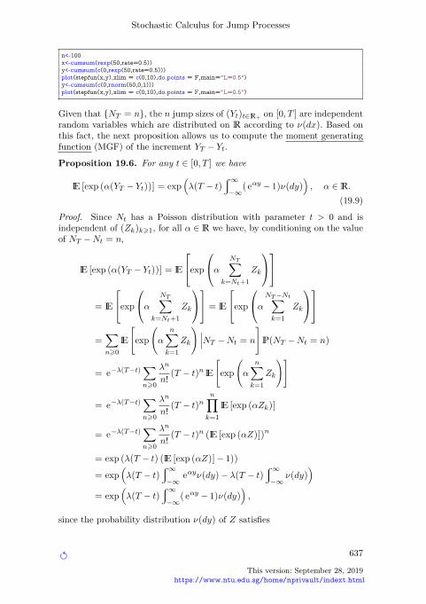
n<-100x<-cumsum(rexp(50,rate=0.5))y<-cumsum(c(0,rexp(50,rate=0.5)))plot(stepfun(x,y),xlim = c(0,10),do.points = F,main="L=0.5")y<-cumsum(c(0,rnorm(50,0,1)))plot(stepfun(x,y),xlim = c(0,10),do.points = F,main="L=0.5")

Given that NT = n, the n jump sizes of (Yt)t∈R+ on [0,T ] are independentrandom variables which are distributed on R according to ν(dx). Based onthis fact, the next proposition allows us to compute the moment generatingfunction (MGF) of the increment YT − Yt.

Proposition 19.6. For any t ∈ [0,T ] we have

IE [exp (α(YT − Yt))] = exp(λ(T − t)

w∞−∞

( eαy − 1)ν(dy))

, α ∈ R.(19.9)

Proof. Since Nt has a Poisson distribution with parameter t > 0 and isindependent of (Zk)k>1, for all α ∈ R we have, by conditioning on the valueof NT −Nt = n,

IE [exp (α(YT − Yt))] = IE

exp

α NT∑k=Nt+1

Zk

= IE

exp

α NT∑k=Nt+1

Zk

= IE

exp

αNT−Nt∑k=1

Zk

=∑n>0

IE[

exp(α

n∑k=1

Zk

)∣∣∣NT −Nt = n

]P(NT −Nt = n)

= e−λ(T−t)∑n>0

λn

n!(T − t)n IE

[exp

(α

n∑k=1

Zk

)]

= e−λ(T−t)∑n>0

λn

n!(T − t)n

n∏k=1

IE [exp (αZk)]

= e−λ(T−t)∑n>0

λn

n!(T − t)n (IE [exp (αZ)])n

= exp (λ(T − t) (IE [exp (αZ)]− 1))

= exp(λ(T − t)

w∞−∞

eαyν(dy)− λ(T − t)w∞−∞

ν(dy))

= exp(λ(T − t)

w∞−∞

( eαy − 1)ν(dy))

,

since the probability distribution ν(dy) of Z satisfies

" 637



N. Privault

IE [exp (αZ)] =w∞−∞

eαyν(dy) andw∞−∞

ν(dy) = 1.

From the moment generating function (19.9) we can compute the expectationof Yt for fixed t as the product of the mean number of jump times IE[Nt] = λtand the mean jump size IE[Z], i.e.,

IE[Yt] =∂

∂αIE[ eαYt ]|α=0 = λt

w∞−∞

yν(dy) = IE[Nt] IE[Z] = λt IE[Z].(19.10)

Note that the above identity requires to exchange the differentiation and ex-pectation operators, which is possible when the moment generating function(19.9) takes finite values for all α in a certain neighborhood (−ε, ε) of 0.

Relation (19.10) states that the mean value of Yt is the mean jump size IE[Z]times the mean number of jumps IE[Nt]. It can also be directly using seriessummations as

IE[Yt] = IE[Nt∑k=1

Zk

]

=∑n>1

IE[

n∑k=1

Zk

∣∣∣Nt = n

]P(Nt = n)

= e−λt∑n>1

λntn

n!IE[

n∑k=1

Zk

∣∣∣Nt = n

]

= e−λt∑n>1

λntn

n!IE[

n∑k=1

Zk

]

= λt e−λt IE[Z]

(λt)n−1(n−1)!∑n>1

= λt IE[Z]= IE[Nt] IE[Z].

Regarding the variance, we have

IE[Y 2t ] =

∂2

∂α2 IE[ eαYt ]|α=0

= λtw∞−∞

y2ν(dy) + (λ(T − t))2(w∞−∞

yν(dy))2

638


"



= λt IE[Z2] + (λt IE[Z])2,

which yields

Var [Yt] = λtw∞−∞

y2ν(dy) = λt IE[|Z|2] = IE[Nt] IE[|Z|2].

As a consequence, the dispersion index of the compound Poisson process

Var [Yt]IE[Yt]

=IE[|Z|2]IE[Z] , t ∈ R+.

is the dispersion index of the random jump size Z. By a multivariate version ofTheorem 22.17, the above identity can be used to show the next proposition.

Proposition 19.7. The compound Poisson process

Yt =Nt∑k=1

Zk, t ∈ R+,

has independent increments, i.e. for any finite sequence of times t0 < t1 <· · · < tn, the increments

Yt1 − Yt0 , Yt2 − Yt1 , . . . , Ytn − Ytn−1

are mutually independent random variables.

Proof. This result relies on the fact that the result of Proposition 19.6 canbe extended to sequences 0 6 t0 6 t1 6 · · · 6 tn and α1,α2, . . . ,αn ∈ R, as

IE[

n∏k=1

eiαk(Ytk−Ytk−1 )

]= IE

[exp

(i

n∑k=1

αk(Ytk − Ytk−1)

)]

= exp(λ

n∑k=1

(tk − tk−1)w∞−∞

( eiαky − 1)ν(dy))

=n∏k=1

exp(λ(tk − tk−1)

w∞−∞

( eiαky − 1)ν(dy))

=n∏k=1

IE[

eiαk(Ytk−Ytk−1 )]

.

Since the compensated compound Poisson process also has independent andcentered increments by (19.6) we have the following counterpart of Proposi-tion 19.4, cf. also Example 2 page 228.

" 639



N. Privault

Proposition 19.8. The compensated compound Poisson process

Mt := Yt − λt IE[Z], t ∈ R+,

is a martingale.

By construction, compound Poisson processes only have a finite number ofjumps on any interval. They belong to the family of Lévy processes whichmay have an infinite number of jumps on any finite time interval, see e.g.§ 4.4.1 of Cont and Tankov (2004).

19.3 Stochastic Integrals with Jumps

Based on the relation∆Yt = ZNt∆Nt,

we can define the stochastic integral of a stochastic process (φt)t∈R+ withrespect to (Yt)t∈R+ by

w T

0φtdYt =

w T

0φtZNtdNt :=

NT∑k=1

φTkZk. (19.11)

As a consequence of Proposition 19.6 we can derive the following version ofthe Lévy-Khintchine formula:

IE[exp

(w T

0f(t)dYt

)]= exp

(λ

w T

0

w∞−∞

( eyf (t) − 1)ν(dy)dt)

for f : [0,T ] −→ R a bounded deterministic function of time.

Note that the expression (19.11) ofw T

0φtdYt has a natural financial interpre-

tation as the value at time T of a portfolio containing a (possibly fractional)quantity φt of a risky asset at time t, whose price evolves according to ran-dom returns Zk, generating profits/losses φTkZk at random times Tk.

In particular the compound Poisson process (Yt)t∈R+ in (19.5) admits thestochastic integral representation

Yt = Y0 +Nt∑k=1

Zk = Y0 +w t

0ZNsdNs.

The next result is also called the smoothing formula, cf. Theorem 9.2.1 inBrémaud (1999).

640


"



Proposition 19.9. Let (φt)t∈R+ be a stochastic process adapted to the fil-tration generated by (Yt)t∈R+ and such that

IE[w T

0|φt|dt

]<∞, T > 0.

The expected value of the compound Poisson compensated stochastic integralcan be expressed as

IE[w T

0φt−dYt

]= IE

[w T

0φt−ZtdNt

]= λ IE[Z] IE

[w T

0φtdt

],

(19.12)

where φt− denotes the left limit

φt− := limst

φs, t > 0.

Proof. By Proposition 19.8 the compensated compound Poisson process (Yt−λt IE[Z])t∈R+ is a martingale, and as a consequence the indefinite stochasticintegral

t 7−→w t

0φs−d(Ys − λ IE[Z]s) =

w t

0φs−(ZNsdNs − λ IE[Z]ds)

is also a martingale, by an argument similar to that in the proof of Propo-sition 7.1 because the adaptedness of (φt)t∈R+ to the filtration generatedby (Yt)t∈R+ , makes (φt−)t>0 predictable, i.e. adapted with respect to thefiltration

Ft− := σ(Ys : s ∈ [0, t)

), t > 0.

It remains to use the fact that the expectation of a martingale remains con-stant over time, which shows that

0 = IE[w T

0φt−(dYt − λ IE[Z]dt)

]= IE

[w T

0φt−dYt

]− λ IE[Z] IE

[w T

0φt−dt

]= IE

[w T

0φt−dYt

]− λ IE[Z] IE

[w T

0φtdt

].

For example, taking φt = Yt := Nt we have

w T

0Nt−dNt =

NT∑k=1

(k− 1) = 12NT (NT − 1),

" 641



N. Privault

henceIE[w T

0Nt−dNt

]=

12(IE[N2T

]− IE[NT ]

)=

(λT )2

2 .

On the other hand, we check that

λ IE[w T

0Nt−dt

]= λ IE

[w T

0Ntdt

]= λ

w T

0IE [Nt] dt

= λ2w T

0tdt

=(λT )2

2 ,

as in (19.12).

Note however that while the identity in expectations (19.12) holds for theleft limit φt− , it need not hold for φt itself. Indeed, taking φt = Yt := Nt wehave

w T

0NtdNt =

NT∑k=1

k =12NT (NT + 1),

hence

IE[w T

0NtdNt

]=

12(IE[N2T

]+ IE[NT ]

)=

12((λT )2 + 2λT

)=

(λT )2

2 + λT

6= λ IE[w T

0Ntdt

].

Under similar conditions, the compound Poisson compensated stochastic in-tegral can be shown to satisfy the Itô isometry (19.13) in the next proposition.

Proposition 19.10. Let (φt)t∈R+ be a stochastic process adapted to thefiltration generated by (Yt)t∈R+ , and such that

IE[w T

0|φt|2dt

]<∞, T > 0.

The expected value of the squared compound Poisson compensated stochasticintegral can be computed as

642


"



IE[(w T


)2]= λ IE[|Z|2] IE

[w T

0|φt|2dt

],

(19.13)

Note that in (19.13), the generic jump size Z is squared but λ is not.

Proof. From the stochastic Fubini-type theorem we have(w T


)2(19.14)

= 2w T

0φt−

w t−

0φs−(dYs − λ IE[Z]ds)(dYt − λ IE[Z]dt) (19.15)

+w T

0|φt− |2|ZNt |

2dNt, (19.16)

where integration over the diagonal s = t has been excluded in (19.15) asthe inner integral has an upper limit t− rather than t. Next, taking expecta-tion on both sides of (19.14)-(19.16) we find

IE[(w T


)2]= IE

[w T

0|φt− |2|ZNt |

2dNt

]= λ IE[|Z|2] IE

[w T

0|φt|2dt

],

where we used the vanishing of the expectation of the double stochastic in-tegral:

IE[w T

0φt−

w t−

0φs−(dYs − λ IE[Z]ds)(dYt − λ IE[Z]dt)

]= 0,

and the martingale property of the compensated compound Poisson process

t 7−→

(Nt∑k=1|Zk|2

)− λt IE[Z2], t ∈ R+,

as in the proof of Proposition 19.9. The isometry relation (19.13) can also beproved using simple predictable processes, similarly to the proof of Proposi-tion 4.16.

Next, take (Bt)t∈R+ a standard Brownian motion independent of (Yt)t∈R+

and (Xt)t∈R+ a jump-diffusion process of the form

Xt :=w t

0usdBs +

w t

0vsds+ Yt, t ∈ R+,

" 643



N. Privault

where (ut)t∈R+ is a stochastic process which is adapted to the filtration(Ft)t∈R+ generated by (Bt)t∈R+ and (Yt)t∈R+ , and such that

IE[w T

0|φt|2|ut|2dt

]<∞ and IE

[w T

0|φtvt|dt

]<∞, T > 0.

We define the stochastic integral of (φt)t∈R+ with respect to (Xt)t∈R+ byw T

0φtdXt :=

w T

0φtutdBt +

w T

0φtvtdt+

w T

0φtdYt

:=w T

0φtutdBt +

w T

0φtvtdt+

NT∑k=1

φTkZk, T > 0.

For the mixed continuous-jump martingale

Xt :=w t

0usdBs + Yt − λt IE[Z], t ∈ R+,

we then have the isometry:

IE[(w T

0φt−dXt

)2]= IE

[w T

0|φt|2|ut|2dt

]+ λ IE[|Z|2] IE

[w T

0|φt|2dt

].

(19.17)

provided that (φs)s∈R+ is adapted to the filtration (Ft)t∈R+ generated by(Bt)t∈R+ and (Yt)t∈R+ . The isometry formula (19.17) will be used in Sec-tion 20.6 for mean-variance hedging in jump-diffusion models.

More generally, when (Xt)t∈R+ contains an additional drift term,

Xt = X0 +w t

0usdBs +

w t

0vsds+

w t

0ηsdYs, t ∈ R+,

the stochastic integral of (φt)t∈R+ with respect to (Xt)t∈R+ is given byw T

0φsdXs :=

w T

0φsusdBs +

w T

0φsvsds+

w T

0ηsφsdYs

=w T

0φsusdBs +

w T

0φsvsds+

NT∑k=1

φTkηTkZk, T > 0.

644


"



19.4 Itô Formula with Jumps

The next proposition gives the simplest instance of the Itô formula withjumps, in the case of a standard Poisson process (Nt)t∈R+ with intensity λ.

Proposition 19.11. Itô formula for the standard Poisson process. We have

f(Nt) = f(0) +w t

0(f(Ns)− f(Ns−))dNs, t ∈ R+,

where Ns− denotes the left limit Ns− = limh0Ns−h.

Proof. We note that

Ns = Ns− + 1 if dNs = 1 and k = NTk = 1 +NT−k

, k > 1.

Hence we have the telescoping sum

f(Nt) = f(0) +Nt∑k=1

(f(k)− f(k− 1))

= f(0) +Nt∑k=1

(f(NTk )− f(NT−k))

= f(0) +Nt∑k=1

(f(1 +NT−k)− f(N

T−k))

= f(0) +w t

0(f(1 +Ns−)− f(Ns−))dNs

= f(0) +w t

0(f(Ns)− f(Ns − 1))dNs

= f(0) +w t

0(f(Ns)− f(Ns−))dNs,

where Ns− denotes the left limit Ns− = limh0Ns−h.

The next result deals with the compound Poisson process (Yt)t∈R+ via asimilar argument.

Proposition 19.12. Itô formula for the compound Poisson process. We havethe pathwise Itô formula

f(Yt) = f(0) +w t

0(f(Ys)− f(Ys−))dNs, t ∈ R+. (19.18)

Proof. We have

f(Yt) = f(0) +Nt∑k=1

(f(YTk )− f(YT−k))

" 645



N. Privault

= f(0) +Nt∑k=1

(f(YT−k+ Zk)− f(YT−

k))

= f(0) +w t

0(f(Ys− + ZNs)− f(Ys−))dNs

= f(0) +w t

0(f(Ys)− f(Ys−))dNs, t ∈ R+.

The formula (19.18) can be decomposed using a compensated Poisson stochas-tic integral as

f(Yt) = f(0) +w t

0(f(Ys)− f(Ys−))(dNs − λds) + λ

w t

0(f(Ys)− f(Ys−))ds.

More generally we have the following result.

Proposition 19.13. For an Itô process of the form

Xt = X0 +w t

0usdBs +

w t

0vsds+

w t

0ηsdYs, t ∈ R+,

we have the Itô formula

f(Xt) = f(X0) +w t

0vsf′(Xs)ds+

w t

0usf′(Xs)dBs +

12

w t

0f ′′(Xs)|us|2ds

+w t

0(f(Xs)− f(Xs−))dNs, t ∈ R+. (19.19)

Proof. By combining the Itô formula for Brownian motion with the aboveargument we find

f(Xt) = f(X0) +w t

0usf′(Xs)dBs +

12

w t

0f ′′(Xs)|us|2ds+

w t

0vsf′(Xs)ds

+

NT∑k=1

(f(XT−k+ ηTkZk

)− f(XT−k

))= f(X0) +

w t

0usf′(Xs)dBs +

12

w t


w t

0vsf′(Xs)ds

+w t

0(f(Xs− + ηsZNs)− f(Xs−))dNs, t ∈ R+,

which yields (19.19).

The integral Itô formula (19.19) can be rewritten in differential notation as

646


"



df(Xt) = vtf′(Xt)dt+utf

′(Xt)dBt+|ut|2

2 f ′′(Xt)dt+(f(Xt)−f(Xt−))dNt,(19.20)

t ∈ R+.

Jump processes with infinite activity

Given an Itô process of the form

Xt := X0 +w t

0usdBs +

w t

0ηsdYt, t ∈ R+,

the Itô formula with jumps (19.19) can be rewritten as

f(Xt) = f(X0) +w t

0vsf′(Xs−)ds+

w t

0usf′(Xs−)dBs

+12

w t


w t

0ηsf′(Xs−)dYs

+w t

0

(f(Xs)− f(Xs−)− ∆Xsf

′(Xs−))dNs, t ∈ R+,

where we used the relation dXs = ηs∆Ys, which impliesw t

0ηsf′(Xs−)dYs =

w t

0∆Xsf

′(Xs−)dNs, t > 0.

The above Poisson stochastic integral can be written asw t

0


′(Xs−))dNs

=w t

0

(f(Xs− + ηs∆Ys)− f(Xs−)− ηs∆Ysf ′(Xs−)

)dNs

=w t

0

(f(Xs− + ηsZNs)− f(Xs−)− ηsZNsf ′(Xs−)

)dNs

=w t

0

(f(Xs− + ηsZ1+Ns− )− f(Xs−)− ηsZNsf ′(Xs−)

)dNs,

and when η(s) is a deterministic function of time, it can be compensated intothe martingalew t

0


′(Xs−))dNs

−w t

0IE[f(x+ η(s)Z)− f(x)− η(s)Zf ′(x)

]x=Xs−

ds

=w t

0

(f(Xs)− f(Xs−)− η(s)Zf ′(Xs−)

)dNs

" 647



N. Privault

−λw t

0

w∞−∞

(f(Xs− + η(s)y)− f(Xs−)− η(s)yf ′(Xs−)

)ν(dy)ds.

This above formulation is at the basis of the extension of Itô’s formula toLévy processes with an infinite number of jumps on any interval, using thebound

|f(x+ y)− f(x)− yf ′(x)| 6 Cy2, y ∈ [−1, 1],

that follows from Taylor’s theorem for f a C2(R) function, cf. e.g. Theo-rem 4.4.7 in Applebaum (2004) in the setting of Poisson random measures.Such processes, also called “infinite activity Lévy processes” are also useful infinancial modeling, Cont and Tankov (2004) and include the gamma process,stable processes, variance gamma processes, inverse Gaussian processes, etc,as in the following illustrations.

1. Gamma process.

0

t

Fig. 19.5: Sample trajectories of a gamma process.

The next R code can be used to generate the gamma process paths ofFigure 19.5.

N=2000; t <- 0:N; dt <- 1.0/N; nsim <- 6; alpha=20.0X = matrix(0, nsim, N)for (i in 1:nsim)X[i,1]=0;X[i,]=rgamma(N,alpha*dt);X <- cbind(rep(0, nsim), t(apply(X, 1, cumsum)))plot(t, X[1, ], xlab = "time", type = "l", ylim = c(0, 2*N*alpha*dt), col = 0)for (i in 1:nsim)points(t, X[i, ], xlab = "time", type = "p", pch=20, cex =0.02, col = i)

648


"



2. Variance gamma process.

0

t

Fig. 19.6: Sample trajectories of a variance gamma process.

3. Inverse Gaussian process.

0

t

Fig. 19.7: Sample trajectories of an inverse Gaussian process.

4. Negative Inverse Gaussian process.

0

t

Fig. 19.8: Sample trajectories of a negative inverse Gaussian process.

" 649



N. Privault

5. Stable process.

0

t

Fig. 19.9: Sample trajectories of a stable process.

The above sample paths of a stable process can be compared to the US-D/CNY exchange rate over the year 2015, according to the date retrievedfrom the following code.

library(quantmod)getSymbols("CNY=X",from="2015-01-01",to="2015-12-6",src="yahoo")rate=Ad(`CNY=X`)chartSeries(rate,up.col="blue",theme="white")

The adjusted close price Ad() is the closing price after adjustments for ap-plicable splits and dividend distributions.

6.20

6.25

6.30

6.35

6.40

rate [2015−01−01/2015−12−04]

Last 6.3875

Jan 012015

Mar 022015

May 012015

Jul 012015

Sep 012015

Nov 022015

Fig. 19.10: USD/CNY Exchange rate data.

Itô multiplication table with jumps

For a stochastic process (Xt)t∈R+ is given by

Xt =w t

0usdBs +

w t

0vsds+

w t

0ηsdNs, t ∈ R+,

the Itô formula with jumps reads

f(Xt) = f(0) +w t

0usf′(Xs)dBs +

12

w t

0|us|2f ′′(Xs)dBs

650


"


https://help.yahoo.com/kb/SLN28256.html


+w t

0vsf′(Xs)ds+

w t

0(f(Xs− + ηs)− f(Xs−))dNs

= f(0) +w t

0usf′(Xs)dBs +

12

w t

0|us|2f ′′(Xs)dBs

+w t

0vsf′(Xs)ds+

w t

0(f(Xs)− f(Xs−))dNs.

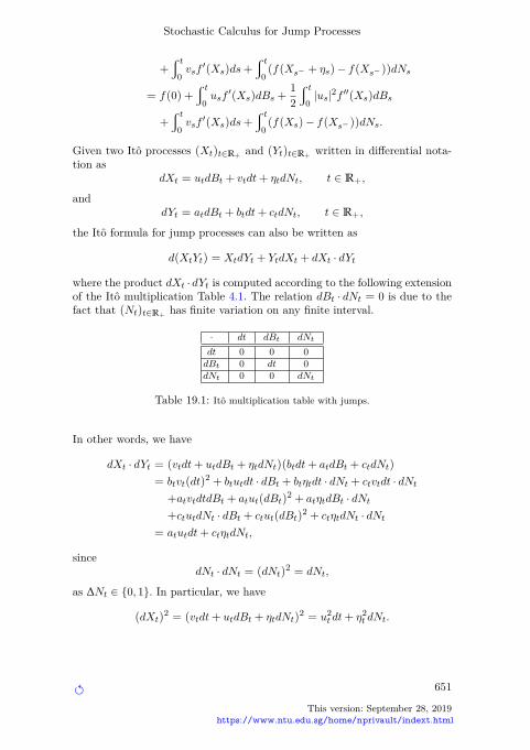
Given two Itô processes (Xt)t∈R+ and (Yt)t∈R+ written in differential nota-tion as

dXt = utdBt + vtdt+ ηtdNt, t ∈ R+,

anddYt = atdBt + btdt+ ctdNt, t ∈ R+,

the Itô formula for jump processes can also be written as

d(XtYt) = XtdYt + YtdXt + dXt · dYt

where the product dXt · dYt is computed according to the following extensionof the Itô multiplication Table 4.1. The relation dBt · dNt = 0 is due to thefact that (Nt)t∈R+ has finite variation on any finite interval.

· dt dBt dNt

dt 0 0 0dBt 0 dt 0dNt 0 0 dNt

Table 19.1: Itô multiplication table with jumps.

In other words, we have

dXt · dYt = (vtdt+ utdBt + ηtdNt)(btdt+ atdBt + ctdNt)

= btvt(dt)2 + btutdt · dBt + btηtdt · dNt + ctvtdt · dNt

+atvtdtdBt + atut(dBt)2 + atηtdBt · dNt

+ctutdNt · dBt + ctut(dBt)2 + ctηtdNt · dNt

= atutdt+ ctηtdNt,

sincedNt · dNt = (dNt)

2 = dNt,

as ∆Nt ∈ 0, 1. In particular, we have

(dXt)2 = (vtdt+ utdBt + ηtdNt)

2 = u2t dt+ η2

t dNt.

" 651



N. Privault

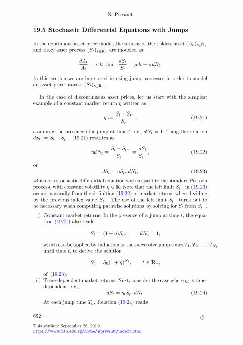
19.5 Stochastic Differential Equations with Jumps

In the continuous asset price model, the returns of the riskless asset (At)t∈R+

and risky asset process (St)t∈R+ are modeled as

dAtAt

= rdt and dStSt

= µdt+ σdBt.

In this section we are interested in using jump processes in order to modelan asset price process (St)t∈R+ .

In the case of discontinuous asset prices, let us start with the simplestexample of a constant market return η written as

η :=St − St−St−

, (19.21)

assuming the presence of a jump at time t, i.e., dNt = 1. Using the relationdSt := St − St− , (19.21) rewrites as

ηdNt =St − St−St−

=dStSt−

, (19.22)

ordSt = ηSt−dNt, (19.23)

which is a stochastic differential equation with respect to the standard Poissonprocess, with constant volatility η ∈ R. Note that the left limit St− in (19.23)occurs naturally from the definition (19.22) of market returns when dividingby the previous index value St− . The use of the left limit St− turns out tobe necessary when computing pathwise solutions by solving for St from St− .

i) Constant market returns. In the presence of a jump at time t, the equa-tion (19.21) also reads

St = (1 + η)St− , dNt = 1,

which can be applied by induction at the successive jump times T1,T2, . . . ,TNtuntil time t, to derive the solution

St = S0(1 + η)Nt , t ∈ R+,

of (19.23).ii) Time-dependent market returns. Next, consider the case where ηt is time-

dependent, i.e.,dSt = ηtSt−dNt. (19.24)

At each jump time Tk, Relation (19.24) reads

652


"



dSTk = STk − ST−k

= ηTkST−k

,

i.e.,STk = (1 + ηTk )ST−

k,

and repeating this argument for all k = 1, 2, . . . ,Nt yields the productsolution

St = S0

Nt∏k=1

(1 + ηTk )

= S0∏

∆Ns=106s6t

(1 + ηs)

= S0∏

06s6t(1 + ηs∆Ns), t ∈ R+.

By a similar argument, we obtain the following proposition.

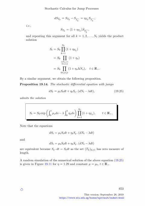
Proposition 19.14. The stochastic differential equation with jumps

dSt = µtStdt+ ηtSt−(dNt − λdt), (19.25)

admits the solution

St = S0 exp(w t

0µsds− λ

w t

0ηsds

) Nt∏k=1

(1 + ηTk ), t ∈ R+.

Note that the equations

dSt = µtStdt+ ηtSt−(dNt − λdt)

anddSt = µtStdt+ ηtSt−(dNt − λdt)

are equivalent because St−dt = Stdt as the set (Tk)k>1 has zero measure oflength.

A random simulation of the numerical solution of the above equation (19.25)is given in Figure 19.11 for η = 1.29 and constant µ = µt, t ∈ R+.

" 653



N. Privault

Fig. 19.11: Geometric Poisson process.∗

The above simulation can be compared to the real sales ranking data ofFigure 19.12.

Fig. 19.12: Ranking data.

Next, consider the equation

dSt = µtStdt+ ηtSt−(dYt − λ IE[Z]dt)

driven by the compensated compound Poisson process (Yt − λ IE[Z]t)t∈R+ ,also written as

dSt = µtStdt+ ηtSt−(ZNtdNt − λ IE[Z]dt),

with solution∗ The animation works in Acrobat Reader on the entire pdf file.

654


"



St = S0 exp(w t

0µsds− λ IE[Z]

w t

0ηsds

) Nt∏k=1

(1 + ηTkZk) t ∈ R+.

(19.26)A random simulation of the geometric compound Poisson process (19.26) isgiven in Figure 19.13.

Fig. 19.13: Geometric compound Poisson process.∗

In the case of a jump-diffusion stochastic differential equation of the form

dSt = µtStdt+ ηtSt−(dYt − λ IE[Z]dt) + σtStdBt,

we get

St = S0 exp(w t

0µsds− λ IE[Z]

w t

0ηsds+

w t

0σsdBs −

12

w t

0|σs|2ds

)×

Nt∏k=1

(1 + ηTkZk), t ∈ R+.

A random simulation of the geometric Brownian motion with compound Pois-son jumps is given in Figure 19.14.∗ The animation works in Acrobat Reader on the entire pdf file.

" 655



N. Privault

Fig. 19.14: Geometric Brownian motion with compound Poisson jumps.∗

By rewriting St as

St = S0 exp(w t

0µsds+

w t

0ηs(dYs − λ IE[Z]ds) +

w t

0σsdBs −

12

w t

0|σs|2ds

)×

Nt∏k=1

((1 + ηTkZk) e−ηTkZk

),

t ∈ R+, one can extend this jump model to processes with an infinite numberof jumps on any finite time interval, cf. Cont and Tankov (2004). The nextFigure 19.15 shows a number of downward and upward jumps occuring inthe SMRT historical share price data, with a typical geometric Brownianbehavior in between jumps.

Fig. 19.15: SMRT Share price.

∗ The animation works in Acrobat Reader on the entire pdf file.

656


"



19.6 Girsanov Theorem for Jump Processes

Recall that in its simplest form, cf. Section 7.2, the Girsanov Theorem forBrownian motion states the following.

Under the probability measure P−µ defined by

dP−µ := e−µBT−µ2T/2dP,

the random variable BT +µT has the centered Gaussian distributionN (0,T ).

This fact follows from the calculation

IE−µ[f(BT + µT )] = IE[f(BT + µT ) e−µBT−µ2T/2]

=1√2πT

w∞−∞

f(x+ µT ) e−µx−µ2T/2 e−x2/(2T )dx

=1√2πT

w∞−∞

f(x+ µT ) e−(x+µT )2/(2T )dx

=1√2πT

w∞−∞

f(y) e−y2/(2T )dy

= IE[f(BT )], (19.27)

for any bounded measurable function f on R, which shows that BT + µT isa centered Gaussian random variable under P−µ.

More generally, the Girsanov Theorem states that (Bt + µt)t∈[0,T ] is a stan-dard Brownian motion under P−µ.

When Brownian motion is replaced with a standard Poisson process (Nt)t∈R+ ,a spatial shift of the type

Bt 7−→ Bt + µt

can no longer be used because Nt + µt cannot be a Poisson process, what-ever the change of probability applied, since by construction, the paths of thestandard Poisson process has jumps of unit size and remain constant betweenjump times.

The correct way to extend the Girsanov Theorem to the Poisson case isto replace the space shift with a shift in the intensity of the Poisson processas in the following statement. Assume that the random variable NT has thePoisson distribution P(λT ) with parameter λT under Pλ.

" 657



N. Privault

Under the probability measure Pλ defined by

dPλ := e−(λ−λ)T(λ

λ

)NTdPλ,

the random variable NT has a Poisson distribution with intensity λT .

This fact follows from the relation

Pλ(NT = k) = e−(λ−λ)T(λ

λ

)kPλ(NT = k) = e−λT λ

k

k!, k ∈N.

Assume now that (Nt)t∈R+ is a standard Poisson process with intensity λunder a probability measure Pλ. In order to extend (19.27) to the Poissoncase we can replace the space shift with a time contraction (or dilation)

Nt 7−→ Nt/(1+c) or Nt 7−→ N(1+c)t,

by a factor 1 + c, where

c := −1 + λ

λ> −1,

or λ = (1 + c)λ. We note that

Pλ

(N(1+c)T = k

)=

(λ(1 + c)T )k

k!e−λ(1+c)T

= (1 + c)k e−λcTPλ(NT = k)

= Pλ(NT = k), k ∈N,

and by analogy with (19.27) we have

IEλ[f(N(1+c)T )

]=∑k>0

f(k)Pλ

(N(1+c)T = k

)(19.28)

= e−λcT∑k>0

f(k)(1 + c)kPλ(NT = k)

= e−λcT IE[f(NT )(1 + c)NT

]= e−λcT

wΩ(1 + c)NT f(NT )dPλ

=w

Ωf(NT )dPλ

= IEλ[f(NT )],

for any bounded function f on N. In other words, taking f(x) := 1x6n wehave658


"



Pλ

(N(1+c)T 6 n

)= Pλ(NT 6 n), n ∈N,

orPλ(NT/(1+c) 6 n) = Pλ

(NT 6 n

), n ∈N.

As a consequence, we have the following proposition.

Proposition 19.15. Let λ, λ > 0, and set

c := −1 + λ

λ> −1.

The process (Nt/(1+c))t∈R+ is a standard Poisson process with intensity λunder Pλ. In particular, the compensated Poisson process

Nt/(1+c) − λt, t ∈ R+,

is a martingale under Pλ.

Proof. As in (19.28) we have

IE[f(NT )] = IEλ[f(NT/(1+c))

],

i.e., under Pλ the distribution of NT/(1+c) is that of a standard Poissonrandom variable with parameter λT . As a consequence, (Nt/(1+c))t∈R+ is astandard Poisson process with intensity λ under Pλ, and since (Nt/(1+c))t∈R+

has independent increments, the compensated process (Nt/(1+c)−λt)t∈R+ isa martingale under Pλ by (7.2).

Similarly, since

(Nt − (1 + c)λt)t∈R+ = (Nt − λt)t∈R+

has independent increments, the compensated Poisson process

Nt − (1 + c)λt = Nt − λt

is a martingale under Pλ. We also have

Nt/(1+c) =∑n>1

1[Tn,∞)(t/(1 + c)) =∑n>1

1[(1+c)Tn,∞)(t), t ∈ R+,

which shows that the jump times ((1+ c)Tn)n>1 of (Nt/(1+c))t∈[0,T ] are dis-tributed under Pλ as the jump times of a Poisson process with intensity λ.

When µ 6= r, the discounted price process (St)t∈R+ = ( e−rtSt)t∈R+ writ-ten as

" 659



N. Privault

dSt

St−= (µ− r)dt+ σ(dNt − λdt) (19.29)

is not a martingale under Pλ. However, we can rewrite (19.29) as

dSt

St−= σ

(dNt −

(λ− µ− r

σ

)dt

)and letting

λ := λ− µ− rσ

= (1 + c)λ

withc := −µ− r

σλ,

we havedSt

St−= σ

(dNt − λdt

)hence the discounted price process (St)t∈R+ is martingale under the proba-bility measure Pλ defined as

dPλ := e−λcT (1 + c)NT dPλ = e(µ−r)/σ(

1− µ− rσλ

)NTdPλ.

We note that ifµ− r < σλ

then the risk-neutral probability measure Pλ exists and is unique, thereforeby Theorems 5.7 and 5.11 the market is without arbitrage and complete.

Girsanov Theorem for compound Poisson processes

In the case of compound Poisson processes, the Girsanov Theorem can beextended to variations in jump sizes in addition to time variations, and wehave the following more general result.

Theorem 19.16. Let (Yt)t>0 be a compound Poisson process with intensityλ > 0 and jump size distribution ν(dx). Consider another intensity parameterλ > 0 and jump size distribution ν(dx), and let

ψ(x) :=λ

λ

ν(dx)

ν(dx)− 1, x ∈ R. (19.30)

Then,

660


"



under the probability measure

dPλ,ν := e−(λ−λ)TNT∏k=1

(1 + ψ(Zk))dPλ,ν ,

the process

Yt :=Nt∑k=1

Zk, t ∈ R+,

is a compound Poisson process with

- modified intensity λ > 0, and

- modified jump size distribution ν(dx).

Proof. For any bounded measurable function f on R, we extend (19.28) tothe following change of variable

IEλ,ν [f(YT )] = e−(λ−λ)T IEλ,ν

f(YT ) NT∏i=1

(1 + ψ(Zi))

= e−(λ−λ)T

∑k>0

IEλ,ν

[f

(k∑i=1

Zi

)k∏i=1

(1 + ψ(Zi))∣∣∣ NT = k

]Pλ(NT = k)

= e−λT∑k>0

(λT )k

k!IEλ,ν

[f

(k∑i=1

Zi

)k∏i=1

(1 + ψ(Zi))

]

= e−λT∑k>0

(λT )k

k!

w∞−∞· · ·

w∞−∞

f(z1 + · · ·+ zk)k∏i=1

(1 + ψ(zi))ν(dz1) · · · ν(dzk)

= e−λT∑k>0

(λT )k

k!

w∞−∞· · ·

w∞−∞

f(z1 + · · ·+ zk)

(k∏i=1

ν(dzi)

ν(dzi)

)ν(dz1) · · · ν(dzk)

= e−λT∑k>0

(λT )k

k!

w∞−∞· · ·

w∞−∞

f(z1 + · · ·+ zk)ν(dz1) · · · ν(dzk).

This shows that under Pλ,ν , YT has the distribution of a compound Poissonprocess with intensity λ and jump size distribution ν. We refer to Propo-sition 9.6 of Cont and Tankov (2004) for the independence of increments of(Yt)t∈R+ under Pλ,ν .

Example. In case ν ' N (α,σ2) and ν ' N (β, η2) we have

" 661



N. Privault

ν(dx) =dx√2πσ2

exp(− 1

2σ2 (x− α)2)

, ν(dx) =dx√2πη2

exp(− 1

2η2 (x− β)2)

,

x ∈ R, hence

ν(dx)

ν(dx)=η

σexp

(1

2η2 (x− β)2 − 1

2σ2 (x− α)2)

, x ∈ R,

and ψ(x) in (19.30) is given by

1 + ψ(x) =λ

λ

ν(dx)

ν(dx)=λη

λσexp

(1

2η2 (x− β)2 − 1

2σ2 (x− α)2)

, x ∈ R.

Note that the compound Poisson process with intensity λ > 0 and jump sizedistribution ν can be built as

Xt :=Nλt/λ∑k=1

h(Zk),

provided that ν is the pushforward measure of ν by the function h : R→ R,i.e.,

P(h(Zk) ∈ A) = P(Zk ∈ h−1(A)) = ν(h−1(A)) = ν(A),

for all (measurable) subsets A of R. As a consequence of Theorem 19.16 wehave the following proposition.

Proposition 19.17. The compensated process

Yt − λt IEν [Z]

is a martingale under the probability measure Pλ,ν defined by

dPλ,ν = e−(λ−λ)TNT∏k=1

(1 + ψ(Zk))dPλ,ν .

Finally, the Girsanov Theorem can be extended to the linear combinationof a standard Brownian motion (Bt)t∈R+ and a compound Poisson process(Yt)t∈R+ independent of (Bt)t∈R+ , as in the following result which is a par-ticular case of Theorem 33.2 of Sato (1999).

Theorem 19.18. Let (Yt)t>0 be a compound Poisson process with intensityλ > 0 and jump size distribution ν(dx). Consider another jump size distri-bution ν(dx) and intensity parameter λ > 0, and let

ψ(x) :=λ

λ

dν

dν(x)− 1, x ∈ R,

662


"



and let (ut)t∈R+ be a bounded adapted process. Then the process(Bt +

w t

0usds+ Yt − λ IEν [Z]t

)t∈R+

is a martingale under the probability measure

dPu,λ,ν = exp(−(λ− λ)T −

w T

0usdBs −

12

w T

0|us|2ds

) NT∏k=1

(1+ψ(Zk))dPλ,ν .

(19.31)

As a consequence of Theorem 19.18, if

Bt +w t

0vsds+ Yt (19.32)

is not a martingale under Pλ,ν , it will become a martingale under Pu,λ,νprovided that u, λ and ν are chosen in such a way that

vs = us − λ IEν [Z], s ∈ R, (19.33)

in which case (19.32) can be rewritten into the martingale decomposition

dBt + utdt+ dYt − λ IEν [Z]dt,

in which both(Bt +

w t

0usds

)t∈R+

and(Yt − λt IEν [Z]

)t∈R+

are martingales

under Pu,λ,ν

When λ = λ = 0, Theorem 19.18 coincides with the usual Girsanov The-orem for Brownian motion, in which case (19.33) admits only one solutiongiven by u = v and there is uniqueness of Pu,0,0. Note that uniqueness occursalso when u = 0 in the absence of Brownian motion with Poisson jumps offixed size a (i.e., ν(dx) = ν(dx) = δa(dx)) since in this case (19.33) alsoadmits only one solution λ = v and there is uniqueness of P0,λ,δa . Theseremarks will be of importance for arbitrage pricing in jump models in Chap-ter 20.

When µ 6= r, the discounted price process (St)t∈R+ = ( e−rtSt)t∈R+ de-fined by

dSt

St−= (µ− r)dt+ σdBt + η(dYt − λt IEν [Z])

is not martingale under Pλ,ν , however we can rewrite the equation as

" 663



N. Privault

dSt

St−= +σ(udt+ dBt) + η

(dYt −

(uσ

η+ λ IEν [Z]−

µ− rη

)dt

)and choosing u, ν, and λ such that

λ IEν [Z] =uσ

η+ λ IEν [Z]−

µ− rη

, (19.34)

we havedSt

St−= σ(udt+ dBt) + η

(dYt − λ IEν [Z]dt

)hence the discounted price process (St)t∈R+ is martingale under the proba-bility measure Pu,λ,ν , and the market is without arbitrage by Theorem 5.7and the existence of a risk-neutral probability measure Pu,λ,ν . However, themarket is not complete due to the non uniqueness of solutions (u, ν, λ) to(19.34), and Theorem 5.11 does not apply in this situation.

Exercises

Exercise 19.1 Consider a standard Poisson process (Nt)t∈R+ with intensityλ > 0, started at N0 = 0.

a) Solve the stochastic differential equation

dSt = ηSt−dNt − ηλStdt = ηSt−(dNt − λdt).

b) Using the first Poisson jump time T1, solve the stochastic differential equa-tion

dSt = −ληStdt+ dNt, t ∈ (0,T2).

Exercise 19.2 Consider a standard Poisson process (Nt)t∈R+ with intensityλ > 0.

a) Solve the stochastic differential equation dXt = αXtdt+ σdNt over thetime intervals [0,T1), [T1,T2), [T2,T3), [T3,T4), where X0 = 1.

b) Write a differential equation for f(t) := IE[Xt], and solve it for t ∈ R+.

Exercise 19.3 Consider a standard Poisson process (Nt)t∈R+ with intensityλ > 0.

a) Solve the stochastic differential equation dXt = σXt−dNt for (Xt)t∈R+ ,where σ > 0 and X0 = 1.

664


"



b) Show that the solution (St)t∈R+ of the stochastic differential equation

dSt = rdt+ σSt−dNt,

is given by St = S0Xt + rXt

w t

0X−1s ds.

c) Compute IE[Xt] and IE[Xt/Xs], 0 6 s 6 t.d) Compute IE[St], t ∈ R+.

Exercise 19.4 Let (Nt)t∈R+ be a standard Poisson process with intensityλ > 0, started at N0 = 0.a) Is the process t 7→ Nt − 2λt a submartingale, a martingale, or a su-

permartingale?b) Let r > 0. Solve the stochastic differential equation

dSt = rStdt+ σSt−(dNt − λdt).

c) Is the process t 7→ St of Question (b) a submartingale, a martingale, or asupermartingale?

d) Compute the price at time 0 of the European call option with strike priceK = S0 e(r−λσ)T , where σ > 0.

Exercise 19.5 Affine stochastic differential equation with jumps. Consider astandard Poisson process (Nt)t∈R+ with intensity λ > 0.a) Solve the stochastic differential equation dXt = adNt + σXt−dNt, where

σ > 0, and a ∈ R.b) Compute IE[Xt] for t ∈ R+.

Exercise 19.6 Consider the compound Poisson process Yt :=Nt∑k=1

Zk, where

(Nt)t∈R+ is a standard Poisson process with intensity λ > 0, and (Zk)k>1 isan i.i.d. sequence of N (0, 1) Gaussian random variables. Solve the stochasticdifferential equation

dSt = rStdt+ ηSt−dYt,

where η, r ∈ R.

Exercise 19.7 Show, by direct computation or using the moment generatingfunction (19.9), that the variance of the compound Poisson process Yt withintensity λ > 0 satisfies

Var [Yt] = λt IE[|Z|2] = λtw∞−∞

x2ν(dx).

" 665



N. Privault

Exercise 19.8 Consider an exponential compound Poisson process of theform

St = S0 eµt+σBt+Yt , t ∈ R+,

where (Yt)t∈R+ is a compound Poisson process of the form (19.7).a) Derive the stochastic differential equation with jumps satisfied by (St)t∈R+ .b) Let r > 0. Find a family (Pu,λ,ν) of probability measures under which the

discounted asset price e−rtSt is a martingale.

Exercise 19.9 Consider (Nt)t∈R+ a standard Poisson process with inten-sity λ > 0 under a probability measure P. Let (St)t∈R+ be defined by thestochastic differential equation

dSt = µStdt+ ZNtSt−dNt, (19.35)

where (Zk)k>1 is an i.i.d. sequence of random variables of the form

Zk = eXk − 1, where Xk ' N (0,σ2), k > 1.

a) Solve the equation (19.35).b) We assume that µ and the risk-free interest rate r > 0 are chosen such

that the discounted process ( e−rtSt)t∈R+ is a martingale under P. Whatrelation does this impose on µ and r?

c) Under the relation of Question (b), compute the price at time t of aEuropean call option on ST with strike price κ and maturity T , using aseries expansion of Black-Scholes functions.

Exercise 19.10 Consider a standard Poisson process (Nt)t∈R+ with intensityλ > 0 under a probability measure P. Let (St)t∈R+ be the mean-revertingprocess defined by the stochastic differential equation

dSt = −αStdt+ σ(dNt − βdt), (19.36)

where S0 > 0 and α,β > 0.a) Solve the equation (19.36) for St.b) Compute f(t) := IE[St] for all t ∈ R+.c) Under which condition on α, β, σ and λ does the process St become a

submartingale?d) Propose a method for the calculation of expectations of the form IE[φ(ST )]

where φ is a payoff function.

Exercise 19.11 Let (Nt)t∈[0,T ] be a standard Poisson process started atN0 = 0, with intensity λ > 0 under the probability measure Pλ, and considerthe compound Poisson process (Yt)t∈[0,T ] with i.i.d. jump sizes (Zk)k>1 ofdistribution ν(dx).666


"



a) Under the probability measure Pλ, the process t 7→ Yt − λt(t+ IE[Z]) isa:

submartingale| martingale| supermartingale|

b) Consider the process (St)t∈[0,T ] given by

dSt = µStdt+ σSt−dYt.

Find λ such that the discounted process (St)t∈[0,T ] := (e−rtSt)t∈[0,T ] is amartingale under the probability measure Pλ defined by its density

dPλ

dPλ:= e−(λ−λ)T

(λ

λ

)NT.

with respect to Pλ.c) Price the forward contract with payoff ST − κ.

Exercise 19.12 Consider (Yt)t∈R+ a compound Poisson process written as

Yt =Nt∑k=1

Zk, t ∈ R+,

where (Nt)t∈R+ a standard Poisson process with intensity λ > 0 and (Zk)k>1is an i.i.d family of random variables with probability distribution ν(dx) onR, under a probability measure P. Let (St)t∈R+ be defined by the stochasticdifferential equation

dSt = µStdt+ St−dYt. (19.37)

a) Solve the equation (19.37).b) We assume that µ, ν(dx) and the risk-free interest rate r > 0 are chosen

such that the discounted process ( e−rtSt)t∈R+ is a martingale under P.What relation does this impose on µ, ν(dx) and r?

c) Under the relation of Question (b), compute the price at time t of aEuropean call option on ST with strike price κ and maturity T , using aseries expansion of integrals.

Exercise 19.13 Consider a standard Poisson process (Nt)t∈[0,T ] with intensityλ > 0 and a standard Brownian motion (Bt)t∈[0,T ] independent of (Nt)t∈[0,T ]under the probability measure Pλ. Let also (Yt)t∈[0,T ] be a compound Poissonprocess with i.i.d. jump sizes (Zk)k>1 of distribution ν(dx) under Pλ, andconsider the jump process (St)t∈[0,T ] solution of

dSt = rStdt+ σStdBt + ηSt−(dYt − λt IE[Z1]).

" 667



N. Privault

with r,σ, η,λ, λ > 0.

a) Assume that λ = λ. Under the probability measure Pλ, the discountedprice process ( e−rtSt)t∈[0,T ] is a:


b) Assume λ > λ. Under the probability measure Pλ, the discounted priceprocess ( e−rtSt)t∈[0,T ] is a:


c) Assume λ < λ. Under the probability measure Pλ, the discounted priceprocess ( e−rtSt)t∈[0,T ] is a:


d) Consider the probability measure Pλ defined by its density

dPλ

dPλ:= e−(λ−λ)T

(λ

λ

)NT.

with respect to Pλ. Under the probability measure Pλ, the discountedprice process ( e−rtSt)t∈[0,T ] is a:


668


"


notes on stochastic finance - ntu.edu.sg · chapter19 stochasticcalculusforjumpprocesses...

Documents