Notes on Decomposition Methods

Stephen Boyd, Lin Xiao, Almir Mutapcic, and Jacob MattingleyNotes for EE364B, Stanford University, Winter 2006-07

April 13, 2008

Contents

1 Primal decomposition 3

1.1 Simple example . . . . . . . . . . . . . . . . . . . . . . . . . . . . . . . . . . 5

2 Dual decomposition 7

2.1 Simple example . . . . . . . . . . . . . . . . . . . . . . . . . . . . . . . . . . 9

3 Decomposition with constraints 11

3.1 Primal decomposition . . . . . . . . . . . . . . . . . . . . . . . . . . . . . . . 113.2 Dual decomposition . . . . . . . . . . . . . . . . . . . . . . . . . . . . . . . . 123.3 Simple example . . . . . . . . . . . . . . . . . . . . . . . . . . . . . . . . . . 133.4 Coupling constraints and coupling variables . . . . . . . . . . . . . . . . . . 15

4 More general decomposition structures 17

4.1 General examples . . . . . . . . . . . . . . . . . . . . . . . . . . . . . . . . . 184.2 Framework for decomposition structures . . . . . . . . . . . . . . . . . . . . 194.3 Primal decomposition . . . . . . . . . . . . . . . . . . . . . . . . . . . . . . . 204.4 Dual decomposition . . . . . . . . . . . . . . . . . . . . . . . . . . . . . . . . 214.5 Example . . . . . . . . . . . . . . . . . . . . . . . . . . . . . . . . . . . . . . 22

5 Rate control 24

5.1 Dual decomposition . . . . . . . . . . . . . . . . . . . . . . . . . . . . . . . . 245.2 Example . . . . . . . . . . . . . . . . . . . . . . . . . . . . . . . . . . . . . . 26

6 Single commodity network flow 28

6.1 Dual decomposition . . . . . . . . . . . . . . . . . . . . . . . . . . . . . . . . 296.2 Analogy with electrical networks . . . . . . . . . . . . . . . . . . . . . . . . . 306.3 Example . . . . . . . . . . . . . . . . . . . . . . . . . . . . . . . . . . . . . . 31

1

Decomposition is a general approach to solving a problem by breaking it up into smallerones and solving each of the smaller ones separately, either in parallel or sequentially. (Whenit is done sequentially, the advantage comes from the fact that problem complexity growsmore than linearly.)

Problems for which decomposition works in one step are called (block) separable, ortrivially parallelizable. As a general example of such a problem, suppose the variable x canbe partitioned into subvectors x1, . . . , xk, the objective is a sum of functions of xi, and eachconstraint involves only variables from one of the subvectors xi. Then evidently we can solveeach problem involving xi separately (and in parallel), and then re-assemble the solution x.Of course this is a trivial, and not too interesting, case.

A more interesting situation occurs when there is some coupling or interaction betweenthe subvectors, so the problems cannot be solved independently. For these cases thereare techniques that solve the overall problem by iteratively solving a sequence of smallerproblems. There are many ways to do this; in this note we consider some simple examplesthat illustrate the ideas.

Decomposition in optimization is an old idea, and appears in early work on large-scaleLPs from the 1960s [DW60]. A good reference on decomposition methods is chapter 6 ofBertsekas [Ber99]. Some recent reference on decomposition applied to networking problemsare Kelly et al [KMT97] and Chiang et al [CLCD07].

The idea of decomposition comes up in the context of solving linear equations, but goesby other names such as block elimination, Schur complement methods, or (for special cases)matrix inversion lemma (see [BV04, App. C]). The core idea, i.e., using efficient methods tosolve subproblems, and combining the results in such a way as to solve the larger problem,is the same, but the techniques are a bit different.

The original primary motivation for decomposition methods was to solve very large prob-lems that were beyond the reach of standard techniques, possibly using multiple processors.This remains a good reason to use decomposition methods for some problems. But otherreasons are emerging as equally (or more) important. In many cases decomposition methodsyield decentralized solution methods. Even if the resulting algorithms are slower (in somecases, much slower) than centralized methods, decentralized solutions might be prefered forother reasons. For example, decentralized solution methods can often be translated into,or interpreted as, simple protocols that allow a collection of subsystems to coordinate theiractions to achieve global optimality.

In §1, we describe the simplest decomposition method, which is called primal decompo-sition since the subsystems coordinate to choose the values of some primal variables. In §2we describe dual decomposition, in which dual variables (prices) are manipulated to solvethe global problem. We explore general decomposition structures, and the associated de-composition methods, in §4. In §5 and §6 we consider two more specific examples in moredetail.

2

1 Primal decomposition

We’ll consider the simplest possible case, an unconstrained optimization problem that splitsinto two subproblems. (But note that the most impressive applications of decompositionoccur when the problem is split into many subproblems.) In our first example, we consideran unconstrained minimization problem, of the form

minimize f(x) = f1(x1, y) + f2(x2, y) (1)

where the variable is x = (x1, x2, y). Although the dimensions don’t matter here, it’s usefulto think of x1 and x2 as having relatively high dimension, and y having relatively smalldimension. The objective is almost block separable in x1 and x2; indeed, if we fix thesubvector y, the problem becomes separable in x1 and x2, and therefore can be solved bysolving the two subproblems independently. For this reason, y is called the complicatingvariable, because when it is fixed, the problem splits or decomposes. In other words, thevariable y complicates the problem. It is the variable that couples the two subproblems. Wecan think of x1 (x2) as the private variable or local variable associated with the first (second)subproblem, and y as the public variable or interface variable or boundary variable betweenthe two subproblems.

The observation that the problem becomes separable when y is fixed suggests a methodfor solving the problem (1). Let φ1(y) denote the optimal value of the problem

minimizex1f1(x1, y), (2)

and similarly, let φ2(y) denote the optimal value of the problem

minimizex2f2(x2, y). (3)

(Note that if f1 and f2 are convex, so are φ1 and φ2.) We refer to (2) as subproblem 1, and(3) as subproblem 2.

Then the original problem (1) is equivalent to the problem

minimizey φ1(y) + φ2(y). (4)

This problem is called the master problem. If the original problem is convex, so is the masterproblem. The variables of the master problem are the complicating or coupling variables ofthe original problem. The objective of the master problem is the sum of the optimal valuesof the subproblems.

A decomposition method solves the problem (1) by solving the master problem, using aniterative method such as the subgradient method. Each iteration requires solving the twosubproblems in order to evaluate φ1(y) and φ2(y) and their gradients or subgradients. Thiscan be done in parallel, but even if it is done sequentially, there will be substantial savings ifthe computational complexity of the problems grows more than linearly with problem size.

Let’s see how to evaluate a subgradient of φ1 at y, assuming the problem is convex. Wefirst solve the associated subproblem, i.e., we find x1(y) that minimizes f1(x1, y). Thus,

3

there is a subgradient of f1 of the form (0, g1), and not surprisingly, g1 is a subgradient of φ1

at y. We can carry out the same procedure to find a subgradient g2 ∈ ∂φ2(y) Then g1 + g2

is a subgradient of φ1 + φ2 at y.We can solve the master problem by a variety of methods, including bisection (if the di-

mension of y is one), gradient or quasi-Newton methods (if the functions are differentiable),or subgradient, cutting-plane, or ellipsoid methods (if the functions are nondifferentiable).This basic decomposition method is called primal decomposition because the master algo-rithm manipulates (some of the) primal variables.

When we use a subgradient method to solve the master problem, we get a very simpleprimal decomposition algorithm.

repeat

Solve the subproblems (possibly in parallel).Find x1 that minimizes f1(x1, y), and a subgradient g1 ∈ ∂φ1(y).Find x2 that minimizes f2(x2, y), and a subgradient g2 ∈ ∂φ2(y).

Update complicating variable.y := y − αk(g1 + g2).

Here αk is a step length that can be chosen in any of the standard ways.We can interpret this decomposition method as follows. We have two subproblems, with

private variables or local variables x1 and x2, respectively. We also have the complicatingvariable y which appears in both subproblems. At each step of the master algorithm thecomplicating variable is fixed, which allows the two subproblems to be solved independently.From the two local solutions, we construct a subgradient for the master problem, and usingthis, we update the complicating variable. Then we repeat the process.

When a subgradient method is used for the master problem, and φ1 and φ2 are differen-tiable, the update has a very simple interpretation. We interpret g1 and g2 as the gradientsof the optimal value of the subproblems, with respect to the complicating variable y. Theupdate simply moves the complicating variable in a direction of improvement of the overallobjective.

The primal decomposition method works well when there are few complicating variables,and we have some good or fast methods for solving the subproblems. For example, if one ofthe subproblems is quadratic, we can solve it analytically; in this case the optimal value isalso quadratic, and given by a Schur complement of the local quadratic cost function. (Butthis trick is so simple that most people would not call it decomposition.)

The basic primal decomposition method described above can be extended in several ways.We can add separable constraints, i.e., constraints of the form x1 ∈ C1, x2 ∈ C2. In this case(and also, in the case when dom fi is not all vectors) we have the possibility that φi(y) = ∞(i.e., y 6∈ dom φ) for some choices of y. In this case we find a cutting-plane that separatesy from domφ, to use in the master algorithm.

4

−1 −0.5 0 0.5 10.5

1

1.5

2

2.5

3

3.5

y

φ1(y)φ2(y)φ1(y) + φ2(y)

Figure 1: Objective function of master problem (i.e., φ1 + φ2) and decomposedcomponents (φ1 and φ2) as a function of y.

1.1 Simple example

We illustrate primal decomposition with a simple example, with a single (scalar) complicatingvariable. The problem has the form (1), where f1 and f2 are piecewise-linear convex functionsof x1 and y, and x2 and y, respectively. For the particular problem instance we consider,x1 ∈ R20, x2 ∈ R20, and f1 and f2 are each the maximum of 100 affine functions. Since thecomplicating variable y is scalar, we can optimize over y using a bisection algorithm.

Figure 1 shows φ1, φ2, and φ1 + φ2 as a function of y. The optimal value of the problemis p⋆ ≈ 1.71, achieved for y⋆ ≈ 0.14. Figure 2 shows the progress of a bisection method forminimizing φ1(y) + φ2(y), with initial interval [−1, 1]. At each step, the two subproblemsare solved separately, using the current value of y.

5

1 2 3 4 5 6 7 810

−4

10−3

10−2

10−1

100

k

f(x

(k) )−

p⋆

Figure 2: Suboptimality versus iteration number k for primal decomposition, withmaster problem solved by bisection.

6

2 Dual decomposition

We can apply decomposition to the problem (1) after introducing some new variables, andworking with the dual problem. We first express the problem as

minimize f(x) = f1(x1, y1) + f2(x2, y2)subject to y1 = y2,

(5)

by introducing a new variable and equality constraint. We have introduced a local version ofthe complicating variable y, along with a consistency constraint that requires the two localversions to be equal. Note that the objective is now separable, with the variable partition(x1, y1) and (x2, y2).

Now we form the dual problem. The Lagrangian is

L(x1, y1, x2, y2, ν) = f1(x1, y1) + f2(x2, y2) + νT y1 − νT y2,

which is separable. The dual function is

g(ν) = g1(ν) + g2(ν),

whereg1(ν) = inf

x1,y1

(

f1(x1, y1) + νT y1

)

, g2(ν) = infx2,y2

(

f2(x2, y2) − νT y2

)

.

Note that g1 and g2 can be evaluated completely independently, e.g., in parallel. Also notethat g1 and g2 can be expressed in terms of the conjugates of f1 and f2:

g1(ν) = −f ∗1 (0,−ν), g2(ν) = −f ∗

2 (0, ν).

The dual problem is

maximize g1(ν) + g2(ν) = −f ∗1 (0,−ν) − f ∗

2 (0, ν), (6)

with variable ν. This is the master problem in dual decomposition. The master algorithmsolves this problem using a subgradient, cutting-plane, or other method.

To evaluate a subgradient of −g1 (or −g2) is easy. We find x1 and y1 that minimizef1(x1, y1) + νT y1 over x1 and y1. Then a subgradient of −g1 at ν is given by −y1. Similarly,if x2 and y2 minimize f2(x2, y2) − νT y2 over x2 and y2, then a subgradient of −g2 at ν isgiven by y2. Thus, a subgradient of the negative dual function −g is given by y2 − y1, whichis nothing more than the consistency constraint residual.

If we use a subgradient method to solve the master problem, the dual decompositionalgorithm has a very simple form.

repeat

Solve the subproblems (possibly in parallel).Find x1 and y1 that minimize f1(x1, y1) + νT y1.Find x2 and y2 that minimize f2(x2, y2) − νT y2.

Update dual variables (prices).ν := ν − αk(y2 − y1).

7

Here αk is a step size which can be chosen several ways. If the dual function g isdifferentiable, then we can choose a constant step size, provided it is small enough. Anotherchoice in this case is to carry out a line search on the dual objective. If the dual function isnondifferentiable, we can use a diminishing nonsummable step size, such as αk = α/k.

At each step of the dual decomposition algorithm, we have a lower bound on p⋆, theoptimal value of the original problem, given by

p∗ ≥ g(ν) = f1(x1, y1) + νT y1 + f2(x2, y2) − νT y2.

where x1, y1, x2, y2 are the iterates. Generally, the iterates are not feasible for the originalproblem, i.e., we have y2−y1 6= 0. (If they are feasible, we have maximized g.) A reasonableguess of a feasible point can be constructed from this iterate as

(x1, y), (x2, y),

where y = (y1 + y2)/2. In other words, we replace y1 and y2 (which are different) with theiraverage value. (The average is the projection of (y1, y2) onto the feasible set y1 = y2.) Thisgives an upper bound on p⋆, given by

p⋆ ≤ f1(x1, y) + f2(x2, y).

A better feasible point can be found by replacing y1 and y2 with their average, and then solv-ing the two subproblems (2) and (3) encountered in primal decomposition, i.e., by evaluatingφ1(y) + φ2(y). This gives the bound

p⋆ ≤ φ1(y) + φ2(y).

Dual decomposition has an interesting economic interpretation. We imagine two sepa-rate economic units, each with its own private variables and cost function, but also withsome coupled variables. We can think of y1 as the amounts of some resources consumedby the first unit, and y2 as the amounts of some resources generated by the second unit.Then, the consistency condition y1 = y2 means that supply is equal to demand. In primaldecomposition, the master algorithm simply fixes the amount of resources to be transferedfrom one unit to the other, and updates these fixed transfer amounts until the total cost isminimized. In dual decomposition, we interpret ν as a set of prices for the resources. Themaster algorithm sets the prices, not the actual amount of the transfer from one unit to theother. Then, each unit independently operates in such a way that its cost, including thecost of the resource transfer (or profit generated from it), is minimized. The dual decompo-sition master algorithm adjusts the prices in order to bring the supply into consistency withthe demand. In economics, the master algorithm is called a price adjustment algorithm, ortatonnement procedure.

There is one subtlety in dual decomposition. Even if we do find the optimal prices ν⋆,there is the question of finding the optimal values of x1, x2, and y. When f1 and f2 are strictlyconvex, the points found in evaluating g1 and g2 are guaranteed to converge to optimal, butin general the situation can be more difficult. (For more on finding the primal solution

8

−1 −0.5 0 0.5 10

0.5

1

1.5

2

2.5

ν

g1(ν)g2(ν)g1(ν) + g2(ν)

Figure 3: Dual functions versus ν.

from the dual, see [BV04, §5.5.5].) There are also some standard tricks for regularizing thesubproblems that work very well in practice.

As in the primal decomposition method, we can encounter infinite values for the sub-problems. In dual decomposition, we can have gi(ν) = −∞. This can occur for some valuesof ν, if the functions fi grow only linearly in yi. In this case we generate a cutting-planethat separates the current price vector from dom gi, and use this cutting-plane to updatethe price vector.

2.1 Simple example

We illustrate dual decomposition with the same simple example used earlier. Figure 3 showsg1, g2, and g1 + g2 as functions of ν. The optimal value of ν is ν⋆ ≈ −0.27. Figure 4 showsthe progress of a bisection method for maximizing g1(ν)+g2(ν), starting from initial interval[−1, 1]. At each step, the two subproblems are solved separately, using the current price ν.We also show two upper bounds on p⋆. The larger (worse) one is f1(x1, y) + f2(x2, y); thesmaller (better) one is φ1(y) + φ2(y) (obtained by solving the subproblems (2) and (3)).

9

0 5 10 151.6

1.7

1.8

1.9

2

2.1

2.2

2.3

2.4

2.5

2.6

k

better boundworse boundg(ν)

Figure 4: Convergence of dual function (lower bound), and simple and better upperbounds.

10

3 Decomposition with constraints

So far, we’ve considered the case where two problems would be separable, except for somecomplicating variables that appear in both subproblems. We can also consider the casewhere the two subproblems are coupled via constraints that involve both sets of variables.As a simple example, suppose our problem has the form

minimize f1(x1) + f2(x2)subject to x1 ∈ C1, x2 ∈ C2

h1(x1) + h2(x2) � 0.(7)

Here C1 and C2 are the feasible sets of the subproblems, presumably described by linearequalities and convex inequalities. The functions h1 : Rn → Rp and h2 : Rn → Rp havecomponents that are convex. The subproblems are coupled via the p constraints that involveboth x1 and x2. We refer to these as complicating constraints (since without them, theproblems involving x1 and x2 can be solved separately).

3.1 Primal decomposition

To use primal decomposition, we can introduce a variable t ∈ Rp that represents the amountof the resources allocated to the first subproblem. As a result, −t is allocated to the secondsubproblem. The first subproblem becomes

minimize f1(x1)subject to x1 ∈ C1, h1(x1) � t,

(8)

and the second subproblem becomes

minimize f2(x2)subject to x2 ∈ C2, h2(x2) � −t.

(9)

Let φ1(t) and φ2(t) denote the optimal values of the subproblems (8) and (8), respectively.Evidently the original problem (7) is equivalent to the master problem of minimizing φ(t) =φ1(t)+φ2(t) over the allocation vector t. These subproblems can be solved separately, whent is fixed.

Not surprisingly, we can find a subgradient for the optimal value of each subproblem froman optimal dual variable associated with the coupling constraint. Let p(z) be the optimalvalue of the convex optimization problem

minimize f(x)subject to x ∈ X, h(x) � z,

and suppose z ∈ dom p. Let λ(z) be an optimal dual variable associated with the constrainth(x) � z. Then, −λ(z) is a subgradient of p at z. To see this, we consider the value of p at

11

another point z:

p(z) = supλ�0

infx∈X

(

f(x) + λT (h(x) − z))

≥ infx∈X

(

f(x) + λ(z)T (h(x) − z))

= infx∈X

(

f(x) + λ(z)T (h(x) − z + z − z))

= infx∈X

(

f(x) + λ(z)T (h(x) − z))

+ λ(z)T (z − z)

= φ(z) + (−λ(z))T (z − z).

This holds for all points z ∈ dom p, so −λ(z) is a subgradient of p at z. (See [BV04, §5.6].)Thus, to find a subgradient of φ, we solve the two subproblems, to find optimal x1 and

x2, as well as optimal dual variables λ1 and λ2 associated with the constraints h1(x1) � t andh2(x2) � −t, respectively. Then we have λ2 −λ1 ∈ ∂φ(t). It is also possible that t 6∈ domφ.In this case we can generate a cutting plane that separates t from domφ, for use in themaster algorithm.

Primal decomposition, using a subgradient master algorithm, has the following simpleform.

repeat

Solve the subproblems (possibly in parallel).Solve (8), to find an optimal x1 and λ1.Solve (9), to find an optimal x2 and λ2.

Update resource allocation.t := t − αk(λ2 − λ1).

Here αk is an appropriate step size. At every step of this algorithm we have points that arefeasible for the original problem.

3.2 Dual decomposition

Dual decomposition for this example is straightforward. We form the partial Lagrangian,

L(x1, x2, λ) = f1(x1) + f2(x2) + λT (h1(x1) + h2(x2))

=(

f1(x1) + λT h1(x1))

+(

f2(x2) + λT h2(x2))

which is separable, so we can minimize over x1 and x2 separately, given the dual variable λ,to find g(λ) = g1(λ) + g2(λ). For example, to find g1(λ), we solve the subproblem

minimize f1(x1) + λT h1(x1)subject to x1 ∈ C1,

(10)

and to find g2(λ), we solve the subproblem

minimize f2(x2) + λT h2(x2)subject to x2 ∈ C2.

(11)

12

A subgradient of −g1 at λ is, naturally, h1(x1), where x1 is any solution of subproblem (10).To find a subgradient of g, the master problem objective, we solve both subproblems,

to get solutions x1 and x2, respectively. A subgradient of −g is then h1(x1) + h2(x2). Themaster algorithm updates (the price vector) λ based on this subgradient.

If we use a projected subgradient method to update λ we get a very simple algorithm.

repeat

Solve the subproblems (possibly in parallel).Solve (10) to find an optimal x1.Solve (11) to find an optimal x2.

Update dual variables (prices).λ := (λ + αk(h1(x1) + h2(x2)))+.

At each step we have a lower bound on p⋆, given by

g(λ) = g1(λ) + g2(λ) = f1(x1) + λT h1(x1) + f2(x2) + λT h2(x2).

The iterates in the dual decomposition method need not be feasible, i.e., we can have h1(x1)+h2(x2) 6� 0. At the cost of solving two additional subproblems, however, we can (often)construct a feasible set of variables, which will give us an upper bound on p⋆. When h1(x1)+h2(x2) 6� 0, we define

t = (h1(x1) − h2(x2))/2, (12)

and solve the primal subproblems (8) and (9). This is nothing more than projecting thecurrent (infeasible) resources used, h1(x1) and h2(x2), onto the set of feasible resource allo-cations, which must sum to no more than 0. As in primal decomposition, it can happen thatt 6∈ domφ. But when t ∈ dom φ, this method gives a feasible point, and an upper boundon p⋆.

3.3 Simple example

We look at a simple example to illustrate decomposition with constraints. The problem isa (strictly convex) QP with a pair of coupling resource constraints. It can be split into twosubproblems, with x1 ∈ R20, x2 ∈ R20. Each subproblem has 100 linear inequalities, and thetwo subproblems share 2 complicating linear inequalities. The optimal value of the problemis p⋆ ≈ −1.33.

Figure 5 shows the progress of primal decomposition for the problem, using a subgradientmethod with step size αk = 0.1. Figure 6 shows the resources consumed by the first of thetwo subproblems.

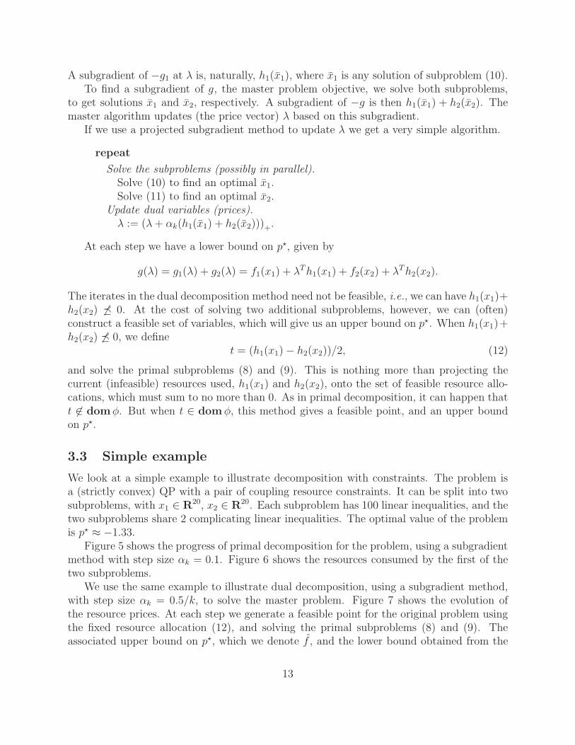
We use the same example to illustrate dual decomposition, using a subgradient method,with step size αk = 0.5/k, to solve the master problem. Figure 7 shows the evolution ofthe resource prices. At each step we generate a feasible point for the original problem usingthe fixed resource allocation (12), and solving the primal subproblems (8) and (9). Theassociated upper bound on p⋆, which we denote f , and the lower bound obtained from the

13

0 20 40 60 80 10010

−4

10−3

10−2

10−1

100

k

f(k

)−

p⋆

Figure 5: Suboptimality versus iteration number k for primal decomposition.

0 20 40 60 80 100−0.2

−0.1

0

0.1

0.2

0.3

0.4

0.5

0.6

0.7

0.8

k

Figure 6: First subsystem resource allocation versus iteration number k for primaldecomposition.

14

0 5 10 15 20 25 300

0.05

0.1

0.15

0.2

0.25

0.3

0.35

0.4

0.45

0.5

k

Figure 7: Resource prices versus iteration number k.

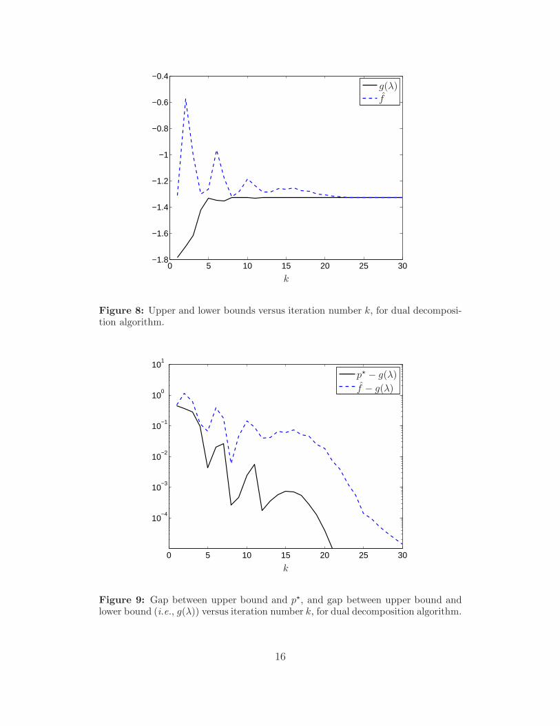
dual function g(λ), are plotted in figure 8. The gap between the best upper and lower boundsis seen to be very small after just 5 iterations or so. Figure 9 shows the actual suboptimalityof f , and the gap between the upper and lower bounds.

3.4 Coupling constraints and coupling variables

Except for the details of computing the relevant subgradients, primal and dual decompositionfor problems with coupling variables and coupling constraints seem quite similar. In fact, wecan readily transform each into the other. For example, we can start with the problem withcoupling constraints (7), and introduce new variables y1 and y2, that bound the subsystemcoupling constraint functions, to obtain

minimize f1(x1) + f2(x2)subject to x1 ∈ C1, h1(x1) � y1

x2 ∈ C2, h2(x2) � −y2

y1 = y2.

(13)

We now have a problem of the form (5), i.e., a problem that is separable, except for aconsistency constraint, that requires two (vector) variables of the subproblems to be equal.

Any problem that can be decomposed into two subproblems that are coupled by somecommon variables, or equality or inequality constraints, can be put in this standard form, i.e.,two subproblems that are independent except for one consistency constraint, that requires asubvariable of one to be equal to a subvariable of the other. Primal or dual decomposition isthen readily applied; only the details of computing the needed subgradients for the masterproblem vary from problem to problem.

15

0 5 10 15 20 25 30−1.8

−1.6

−1.4

−1.2

−1

−0.8

−0.6

−0.4

k

g(λ)

f

Figure 8: Upper and lower bounds versus iteration number k, for dual decomposi-tion algorithm.

0 5 10 15 20 25 30

10−4

10−3

10−2

10−1

100

101

k

p⋆ − g(λ)

f − g(λ)

Figure 9: Gap between upper bound and p⋆, and gap between upper bound andlower bound (i.e., g(λ)) versus iteration number k, for dual decomposition algorithm.

16

1 2

Figure 10: Simplest decomposition structure.

1 2 3

Figure 11: Chain structure, with three subsystems and two coupling constraints.

4 More general decomposition structures

So far we have studied the case where there are two subsystems that are coupled by sharedvariables, or coupling constraints. Clearly we can have more than one subproblem, withvarious subsets of them coupled in various ways. For example, the variables might be par-titioned into subvectors, some of which are local (i.e., appear in one subproblem only) andsome of which are complicating (i.e., appear in more than one subproblem). This decom-position structure can be represented by a hypergraph. The nodes are associated with thesubproblems, which involve local variables, objective terms, and local constraints. The hy-peredges or nets are associated with complicating variables or constraints. If a hyperedgeis adjacent to only two nodes, we call it a link. A link corresponds to a shared variable orconstraint between the two subproblems represented by the nodes. The simplest possibledecomposition structure consists of two subsystems and some coupling between them, asshown in figure 10. In this figure the subsystems are shown as the boxes labeled 1 and 2;the coupling between them is shown as the link connecting the boxes.

Figure 11 shows another simple decomposition structure with three subsystems, labeled1, 2, and 3. This problem consists of three subproblems, with some coupling between sub-problems 1 and 2, and some coupling between subproblems 2 and 3. Adopting the canonicalform for coupling, i.e., as consistency constraints, we can write the associated problem as

minimize f1(x1, y1) + f2(x2, y2, y3) + f3(x3, y4)subject to (x1, y1) ∈ C1, (x2, y2, y3) ∈ C2, (x3, y4) ∈ C3

y1 = y2, y3 = y4.

Subsystem 1 has private or local variable x1, and public or interface variable y1. Subsystem 2has local variable x2, and interface variables y2 and y3. Subsystem 3 has local variable x3, andinterface variable y4. This decomposition structure has two edges: the first edge correspondsto the consistency constraint y1 = y2, and the second edge corresponds to the consistencyconstraint y3 = y4.

17

1 2

3 4 5

c1

c2

c3 c4

Figure 12: A more complex decomposition structure with 5 subsystems and 4coupling constraints.

A more complex decomposition structure is shown in figure 12. This consists of 5 sub-systems and 4 coupling constraints. Coupling constraint c1, for example, requires that threepublic variables of subsystem 1, 2, and 3 should all be equal.

We will give the details later, but we describe, roughly, how primal and dual decompo-sition works in the more general setting with complex decomposition structure. In primaldecomposition, each hyperedge or net has a single variable associated with it. Each subsys-tem is optimized separately, using the public variable values (asserted) on the nets. Eachsubsystem produces a subgradient associated with each net it is adjacent to. These arecombined to update the variable value on the net, hopefully in such a way that convergenceto (global) optimality occurs.

In dual decomposition, each subsystem has its own private copy of the public variableson the nets it is adjacent to, as well as an associated price vector. The subsystems use theseprices to optimize their local variables, including the local copies of public variables. Thepublic variables on each net are then compared, and the prices are updated, hopefully ina way that brings the local copies of public variables into consistency (and therefore alsooptimality).

4.1 General examples

Before introducing some formal notation for decomposition structures, we informally describea few general examples.

In an optimal control problem, the state at time t is the complicating variable between thepast (i.e., variables associated with time before t) and the future (variables associated withtime after t). In other words, if you fix the state in a dynamical system, the past and futurehave nothing to do with each other. (That’s exactly what it means to be a state.) In termsof a decomposition graph, we have nodes associated with the system at times t = 1, . . . , T ;

18

each node is coupled to the node before and after, by the state equations. Thus, the optimalcontrol problem decomposition structure is represented by a simple linear chain.

Decomposition structure arises in many applications in network optimization. For exam-ple, we can partition a network into subnetworks, that interact only via common flows, ortheir boundary connections. We can partition a multi-commodity flow problem into a set ofsingle-commodity flow problems coupled by shared resources. the capacities of the links. Ina flow control problem, we can view each flow in a network as a subsystem; these flows arecoupled by sharing the capacities of the links.

In some image processing problems, variables associated with pixels are only coupled tothe variables associated with some of their neighbors. In this case, any strip with a widthexceeding the interaction distance between pixels, and which disconnects the image planecan be taken as a set of complicating variables. You can solve an image restoration problem,then, by fixing a strip (say, down the middle), and then (in parallel) solving the left andright image problems. (This can clearly be done recursively as well.)

Decomposition structure arises in hierarchical design. Suppose we are designing (viaconvex optimization) a large circuit (say) that consists of some subcircuits. Each subcircuithas many private variables, and a few variables that interact with other subcircuits. Forexample, the device dimensions inside each subcircuit might be local or private variables;the shared variables correspond to electrical connections between the subcircuits (e.g., theload presented to one subcircuit from another) or objectives or constraint that couple them(e.g., a total power or area limit). At each step of algorithm in primal decomposition, wefix the coupling variables, and then design the subcircuits (separately) to meet these fixedspecifications on their boundaries. We then update the coupling variables in such a way thatthe total cost (say, power) eventually is minimized. In dual decomposition, we allow eachsubcircuit to choose its own values for its boundary variables, but add an extra cost, basedon prices, to account for its effects on the overall circuit. These prices are updated to bringthe design into consistency.

4.2 Framework for decomposition structures

In this section we describe decomposition with a general structure in more detail. We have Ksubsystems. Subsystem i has private variables xi ∈ Rni , public variables yi ∈ Rpi, objectivefunction fi : Rni × Rpi, and local constraint set Ci ⊆ Rni × Rpi. The overall objective is∑K

i=1 fi(xi, yi), and the local constraints are (xi, yi) ∈ Ci.These subsystems are coupled through constraints that require various subsets of the

components of the public variables to be equal. (Each of these subsets corresponds to ahyperedge or net in the decomposition structure.) To describe this we collect all the publicvariables together into one vector variable y = (y1, . . . , yK) ∈ Rp, where p = p1 + · · · + pK

is the total number of (scalar) public variables. We use the notation (y)i to denote the ith(scalar) component of y, for i = 1, . . . , p (in order to distinguish it from yi, which refers tothe portion of y associated with subsystem i).

We suppose there are N nets, and we introduce a vector z ∈ RN that gives the commonvalues of the public variables on the nets. We can express the coupling constraints as y = Ez,

19

where E ∈ Rp×N is the matrix with

Eij =

{

1 (y)i is in net j0 otherwise.

The matrix E specifies the netlist, or set of hyperedges, for the decomposition structure. Wewill let Ei ∈ Rpi×N denote the partitioning of the rows of E into blocks associated with thedifferent subsystems, so that yi = Eiz. The matrix Ei is a 0-1 matrix that maps the vectorof net variables into the public variables of subsystem i.

Our problem then has the form

minimize∑K

i=1 fi(xi, yi)subject to (xi, yi) ∈ Ci, i = 1, . . . , K

yi = Eiz, i = 1, . . . , K,(14)

with variables xi, yi, and z. We refer to z as the vector of (primal) net variables.

4.3 Primal decomposition

In primal decomposition, at each iteration we fix the vector z of net variables, and we fix thepublic variables as yi = Eiz. The problem is now separable; each subsystem can (separately)find optimal values for its local variables xi. Let φi(yi) denote the optimal value of thesubproblem

minimize fi(xi, yi)subject to (xi, yi) ∈ Ci,

(15)

with variable xi, as a function of yi. The original problem (14) is equivalent to the primalmaster problem

minimize φ(z) =∑K

i=1 φi(Eiz),

with variable z. To find a subgradient of φ, we find gi ∈ ∂φi(yi) (which can be doneseparately). We then have

g =K

∑

i=1

ETi gi ∈ ∂φ(z).

This formula has a simple interpretation: To find a subgradient for the net variable zi, wecollect and sum the subgradients over all components of the public variables adjacent tonet i.

If the master problem is solved using a subgradient method, we have the following algo-rithm.

repeat

Distribute net variables to subsystems.yi := Eiz, i = 1, . . . , K.

Optimize subsystems (separately).Solve subproblems (15) to find optimal xi, and gi ∈ ∂φi(yi), i = 1, . . . , K.

20

Collect and sum subgradients for each net.g :=

∑Ki=1 ET

i gi.Update net variables.

z := z − αkg.

Here αk is an appropriate step size. This algorithm is decentralized: at each step, the actionstaken involve only the subsystems, which act independently of each other, or the nets, whichact independently of each other. The only communication is between subsystems and thenets they are adjacent to. There is no communication between (or, to anthropomorphize abit, any awareness of) different subsystems, or different nets.

4.4 Dual decomposition

We form the partial Lagrangian of problem (14),

L(x, y, z, ν) =K

∑

i=1

fi(xi, yi) + νT (y − Ez)

=K

∑

i=1

(

fi(xi, yi) + νTi yi

)

− νT Ez,

where ν ∈ Rp is the Lagrange multiplier associated with y = Ez, and νi is the subvectorof ν associated with the ith subsystem. To find the dual function we first minimize over z,which results in the condition ET ν = 0 for g(ν) > −∞. This condition states that for eachnet, the sum of the Lagrange multipliers over the net is zero. We define gi(νi) as the optimalvalue of the subproblem

minimize fi(xi, yi) + νTi yi

subject to (xi, yi) ∈ Ci,(16)

as a function of νi. A subgradient of −gi at νi is just −yi, an optimal value of yi in thesubproblem (16).

The dual of the original problem (14) is

maximize g(ν) =∑K

i=1 gi(νi)subject to ET ν = 0,

with variable ν.We can solve this dual decomposition master problem using a projected subgradient

method. Projection onto the feasible set {ν | ET ν = 0}, which consists of vectors whosesum over each net is zero, is easy to work out. The projection is given by multiplication byI − E(ET E)−1ET , which has a particularly simple form, since

ET E = diag(d1, . . . , dN),

where di is the degree of net i, i.e., the number of subsystems adjacent to net i. For u ∈ Rp,(ET E)−1Eu gives the average, over each net, of the entries in the vector u. The vector

21

(ET E)−1Eu is the vector obtained by replacing each entry of u with its average over itsassociated net. Finally, projection of u onto the feasible set is obtained by subtracting fromeach entry the average of other values in the associated net.

Dual decomposition, with a subgradient method for the master problem, gives the fol-lowing algorithm.

given initial price vector ν that satisfies ET ν = 0 (e.g., ν = 0).

repeat

Optimize subsystems (separately).Solve subproblems (16) to obtain xi, yi.

Compute average value of public variables over each net.z := (ET E)−1ET y.

Update prices on public variables.ν := ν + αk(y − Ez).

Here αk is an appropriate step size. This algorithm, like the primal decomposition algo-rithm, is decentralized: At each step, the actions taken involve only the subsystems, actingindependently of each other, or the nets, acting independently of each other.

We note that z, computed in the second step, gives a reasonable guess for z⋆, the optimalnet variables. If we solve the primal subproblems (15), using yi = Eiz, we obtain a feasiblepoint, and an associated upper bound on the optimal value.

The vector y − Ez = (I − E(ET E)−1ET )y, computed in the last step, is the projectionof the current values of the public variables onto the set of feasible, or consistent values ofpublic variables, i.e., those that are the same over each net. The norm of this vector givesa measure of the inconsistency of the current values of the public variables.

4.5 Example

Our example has the structure shown in figure 12. Each of the local variables has dimension10, and all 9 public variables are scalar, so all together there are 50 private variables, 9 publicvariables, and 5 linear equality constraints. (The hyperedge labeled c1 requires that threepublic variables be equal, so we count it as two linear equality constraints.) Each subsystemhas an objective term that is a convex quadratic function plus a piecewise-linear function.There are no local constraints. The optimal value of the problem is p⋆ ≈ 11.1.

We use dual decomposition with fixed step size α = 0.5. At each step, we compute twofeasible points. The simple one is (x, y), with y = Ez. The more costly, but better, point is(x, y) where x is found by solving the primal decomposition subproblems using y. Figure 13shows g(ν), and the objectove for the two feasible points, f(x, y) and f(x, y), versus iterationnumber. Figure 14 shows ‖y − Ez‖, the norm of the consistency constraint residual, versusiteration number.

22

0 2 4 6 8 10 129

10

11

12

13

14

15

16

17

18

k

g(ν)

f(x, y)f(x, y)

Figure 13: Upper and lower bounds versus iteration number k, for dual decompo-sition algorithm.

0 2 4 6 8 10 1210

−2

10−1

100

101

k

‖y−

Ez‖

Figure 14: Norm of the consistency constraint residual, ‖y −Ez‖, versus iterationnumber k, for dual decomposition algorithm.

23

5 Rate control

There are n flows in a network, each of which passes over a fixed route, i.e., some subset ofm links. Each flow has a nonnegative flow rate or rate, which we denote f1, . . . , fn. Withflow j we associate a utility function Uj : R → R, which is strictly concave and increasing,with domUj ⊆ R+. The utility derived by a flow rate fj is given by Uj(fj). The total utilityassociated with all the flows is then U(f) = U1(f1) + · · ·+ Un(fn).

The total traffic on a link in the network, denoted t1, . . . , tm, is the sum of the rates of allflows that pass over that link. We can express the link traffic compactly using the routingor link-route matrix R ∈ Rm×n, defined as

Rij =

{

1 flow j passes over link i0 otherwise,

as t = Rf . Each link in the network has a (positive) capacity c1, . . . , cm. The traffic on alink cannot exceed its capacity, i.e., we have Rf � c.

The flow rate control problem is to choose the rates to maximize total utility, subject tothe link capacity constraints:

maximize U(f)subject to Rf � c,

(17)

with variable f ∈ Rn. This is evidently a convex optimization problem.We can decompose the rate control problem in several ways. For example, we can view

each flow as a separate subsystem, and each link capacity constraint as a complicatingconstraint that involves the flows that pass over it.

5.1 Dual decomposition

The Lagrangian (for the problem of minimizing −U) is

L(f, λ) = −n

∑

j=1

Uj(fj) + λT (Rf − c),

and the dual function is given by

g(λ) = inff

n∑

j=1

−Uj(fj) + λT (Rf − c)

= −λT c +n

∑

j=1

inffj

(−Uj(fj) + (rTj λ)fj)

= −λT c −n

∑

j=1

(−Uj)∗(rT

j λ),

where rj is the jth column of R. The number rTj λ is the sum of the Lagrange multipliers

associated with the links along route j.

24

The dual problem is

maximize −λT c − ∑nj=1(−Uj)

∗(−rTj λ)

subject to λ � 0.(18)

A subgradient of −g is given by Rf − c, where fj is a solution of the subproblem

minimize −Uj(fj) + (rTj λ)fj,

with variable fj . (The constraint fj ≥ 0 is implicit here.)Using a projected subgradient method to solve the dual problem, we obtain the following

algorithm.

given initial link price vector λ ≻ 0 (e.g., λ = 1).

repeat

Sum link prices along each route.Calculate Λj = rT

j λ.Optimize flows (separately) using flow prices.

fj := argmax (Uj(fj) − Λjfj).Calculate link capacity margins.

s := c − Rf .Update link prices.

λ := (λ − αks)+.

Here αk is an appropriate stepsize.This algorithm is completely decentralized: Each flow is updated based on information

obtained from the links it passes over, and each link price is updated based only on the flowsthat pass over it. The algorithm is also completely natural. We can imagine that a flow ischarged a price λl (per unit of flow) for passing over link i. The total charge for the flow isthen Λjfj . This charge is subtracted from its utility, and the maximum net utility flow ratechosen. The links update their prices depending on their capacity margin s = c − t, wheret = Rf is the link traffic. If the margin is positive, the link price is decreased (but not belowzero). If the margin is negative, which means the link capacity constraint is violated, thelink price is increased.

The flows at each step of the algorithm can violate the capacity constraints. We cangenerate a set of feasible flows by fixing an allocation of each link capacity to each flow thatpasses through it, and then optimizing the flows. Let η ∈ Rm be the factors by which thelink traffic exceeds link capacity, i.e., ηi = ti/ci, where t = Rf is the traffic. If ηi ≤ 1, link iis operating under capacity; if ηi > 1, link i is operating over capacity. Define f feas as

f feasj =

fj

max{ηi | flow j passes over link i} , j = 1, . . . , n. (19)

This flow vector will be feasible. Roughly speaking, each flow is backed off by the maximumover capacity factor over its route. (If all links on a route are under-utilized, this schemewill actually increase the flow.)

25

0 20 40 60 80 100−22

−21

−20

−19

−18

−17

−16

k

U(f feas)−g(λ)

Figure 15: Upper bound −g(λ) and lower bound U(f feas) on optimal utility, versusiteration k.

5.2 Example

We consider an example with n = 10 flows and m = 12 links. The number of links perflow is either 3 or 4, and the number of flows per link is around 3. The link capacitiesare chosen randomly, uniformly distributed on [0.1, 1]. We use a log utility function, i.e.,Uj(fj) = log fj . (This can be argued to achieve fairness among the flows.) The optimal flow,as a function of price, is

argmax (Uj(fj) − Λjfj) = 1/Λj.

We initialize the link prices at λ = 1, and use a constant stepsize αk = 3. (The dual functiong is differentiable, so a small enough constant step size with result in convergence.)

Figure 15 shows the evolution of the dual decomposition method. The upper plot showsthe bound −g(λ) on the optimal utility. The bottom plot shows the utility achieved bythe feasible flow found from (19). Figure 16 shows the evolution of the maximum capacityviolation, i.e., maxi(Rf − c)i.

26

0 20 40 60 80 10010

−2

10−1

100

max

i(R

f−

c)i

k

Figure 16: Maximum capacity violation versus iteration k.

27

6 Single commodity network flow

We consider a connected directed graph or network with n edges and p nodes. We let xj

denote the flow or traffic on arc j, with xj > 0 meaning flow in the direction of the arc, andxj < 0 meaning flow in the direction opposite the arc. There is also a given external source(or sink) flow si that enters (if si > 0) or leaves (if si < 0) node i. The flow must satisfya conservation equation, which states that at each node, the total flow entering and leavingthe node, including the external sources and sinks, is zero. This conservation equation canbe expressed as Ax + s = 0 where A ∈ Rp×n is the node incidence matrix of the graph,

Aij =

1 arc j enters i−1 arc j leaves node i

0 otherwise.

Thus, each column of A describes a link; it has exactly two nonzero entries (one equal to 1and the other equal to −1) indicating the end and start nodes of the link respectively. Eachrow of A describes all links incident to a node: the +1 entries indicate incoming links andthe −1 entries indicate outgoing links.

The flow conservation equation Ax + s = 0 is inconsistent unless 1T s = 0, which weassume is the case. (In other words, the total of the source flows must equal the totalof the sink flows.) The flow conservation equations Ax + s = 0 are also redundant, since1T A = 0. To obtain an independent set of equations we can delete any one equation, toobtain Ax + s = 0, where A ∈ R(p−1)×n is the reduced node incidence matrix of the graph(i.e., the node incidence matrix with one row removed) and s ∈ Rp−1 is reduced sourcevector (i.e., s with the associated entry removed).

We will take traffic flows x as the variables, and the sources and network topology asgiven. We introduce the separable objective function

φ(x) =n

∑

j=1

φj(xj),

where φj : R → R is the flow cost function for arc j. We assume that the flow cost functionsare strictly convex. We can impose other limits on the flow variables, e.g., the conditionxj ≥ 0 that flows must be in the direction of the arcs, by restricting the domain of the arccost functions.

The problem of choosing the minimum cost flow that satisfies the flow conservationrequirement is formulated as

minimize∑n

j=1 φj(xj)subject to Ax + s = 0.

(20)

This problem is also called the single commodity network flow problem.The single commodity network flow problem is convex, and readily solved by standard

methods, such as Newton’s method (when φj are twice differentiable). Using dual decompo-sition, however, we obtain a decentralized method for solving the problem.

28

6.1 Dual decomposition

The Lagrangian is

L(x, ν) = φ(x) + νT (Ax + s)

= νT s +n

∑

j=1

(

φj(xj) + (aTj ν)xj

)

,

where aj is the jth column of A. We use the notation ∆νj to denote aTj ν, since it is the

difference of the dual variable between the ending node and starting node of arc j. We willsee that the dual variables νi can be interpreted as potentials on the network; ∆νj is thepotential difference appearing across arc j.

The dual function is

g(ν) = infx

L(x, ν)

= νT s +n

∑

j=1

infxj

(φj(xj) + (∆νj)xj)

= νT s −n

∑

j=1

φ∗j(−∆νj),

where φ∗j is the conjugate function of φj , i.e.,

φ∗j(y) = sup

x(yxj − φj(xj)) .

The dual problem is the unconstrained convex problem

maximize g(ν),

with variable ν ∈ Rp. It is easy to show that only differences in the potentials matter; wehave g(ν) = g(ν + c1) for any c ∈ R. We can, without loss of generality, fix one of the dualvariables to be zero.

There is no duality gap; the optimal values of the primal and dual problems are the same.Moreover, we can recover the primal solution from the dual solution. Since we assume the flowcost functions φj are strictly convex, for each y there is a unique maximizer of yxj − φj(xj).We will denote this maximizer as x∗

j (y). If φj is differentiable, then x∗j (y) = (φ′

j)−1(y), the

inverse of the derivative function. We can solve the network flow problem via the dual, asfollows. We first solve the dual by maximizing g(ν) over ν to obtain the optimal dual variable(or potentials) ν⋆. Then the optimal solution of the network flow problem is given by

x⋆j = x∗

j (−∆ν⋆j ).

Thus, the optimal flow on link j is a function of the optimal potential difference across it.In particular, the optimal flow can be determined locally; we only need to know the optimalpotential values at the two adjacent nodes to find the optimal flow on the arc.

29

A subgradient for the negative dual function −g is

−(Ax∗(∆ν) + s) ∈ ∂(−g)(ν).

This is exactly the negative of the flow conservation residual. The ith component of theresidual,

aTi x∗(∆ν) + si,

is sometimes called the flow surplus at node i, since it is the difference between the totalincoming and total outgoing flow at node i. Using a subgradient method to solve the dual,we obtain the following algorithm.

given initial potential vector ν.

repeat

Determine link flows from potential differences.xj := x∗

j (−∆νj), j = 1, . . . , n.Compute flow surplus at each node.

Si := aTi x + si, i = 1, . . . , p.

Update node potentials.νi := νi + αkSi, i = 1, . . . , p.

Here αk > 0 is an appropriate step length.The method proceeds as follows. Given the current value of the potentials, a flow is

calculated. This is local; to find xj we only need to know the two potential values at theends of arc j. We then compute the flow surplus at each node. Again, this is local; to findthe flow surplus at node i, we only need to know the flows on the arcs that enter or leavenode i. Finally, we update the potentials based on the current flow surpluses. The updateis very simple: we increase the potential at a node with a positive flow surplus (recall thatflow surplus is −gi at node i), which (we hope) will result in reduced flow into the node.Provided the step length αk can be computed locally, the algorithm is distributed; the arcsand nodes only need information relating to their adjacent flows and potentials. There is noneed to know the global topology of the network, or any other nonlocal information, such aswhat the flow cost functions are.

At each step of the dual subgradient method, g(ν) is a lower bound on p⋆, the optimalvalue of the single-commodity network flow problem. (Note, however, that computing thislower bound requires collecting information from all arcs in the network.) The iterates aregenerally infeasible, i.e., we have Ax + s 6= 0. The flow convervation constraint Ax + s = 0is satisfied only in the limit as the algorithm converges.

There are methods to construct a feasible flow from x, an infeasible iterate of the dualsubgradient method. Projecting onto the feasible set, defined by Ax + s = 0, can be doneefficiently but is not decentralized.

6.2 Analogy with electrical networks

There is a nice analogy between the single commodity network flow problem and electricalnetworks. We consider an electrical network with topology determined by A. The variable

30

xj is the current flow in branch j (with positive indicating flow in the reference direction,negative indicating current flow in the opposite direction). The source si is an externalcurrent injected at node i. Naturally, the sum of the external currents must be zero. Theflow conservation equation Ax + s = 0 is Khirchhoff’s current law (KCL).

The dual variables correspond to the node potentials in the circuit. We can arbitrarilychoose one node as the ground or datum node, and measure potentials with respect to thatnode. The potential difference ∆νj is precisely the voltage appearing across the jth branchof the circuit. Each branch in the circuit contains a nonlinear resistor, with current-voltagecharacteristic Ij = x∗

j (−Vj).It follows that the optimal flow is given by the current in the branches, with the topology

determined by A, external current s, and current-voltage characteristics related to the flowcost functions. The node potentials correspond to the optimal dual variables. (It has beensuggested to solve optimal flow equations using analog circuits.)

The subgradient algorithm gives us an iterative way to find the currents and voltages insuch a circuit. The method updates the node potentials in the circuit. For a given set of nodepotentials we calculate the branch currents from the branch current-voltage characteristics.Then we calculate the KCL residual, i.e., the excess current at each node, and update thepotentials based on these mismatches. In particular, we increase the node potential at eachnode which has too much current flowing into it, and decrease the potential at each nodewhich has too little current flowing into it. (For constant step size, the subgradient methodcorresponds roughly to putting a capacitor to ground at each node.)

6.3 Example

We now consider a more specific example, with flow cost function

φj(xj) =xj

cj − xj

, domφj = [0, cj),

where cj > 0 are given link capacities. The domain restrictions mean that each flow isnonnegative, and must be less than the capacity of the link. This function gives the ex-pected queuing delay in an M/M/1 queue, with exponential arrival times with rate xj andexponential service time with rate cj .

The conjugate of this function is

φ∗j(y) =

{

(√

cjy − 1)2 y > 1/cj

0 y ≤ 1/cj.

The function and its conjugate are plotted in figure 17, for c = 1.From the conjugate we can work out the function x∗

j (−∆νj):

x∗j = argmin

0≤z<cj

(φj(z) + ∆νjz) =

{

cj −√

cj/∆νj ∆νj > 1/cj

0 ∆νj ≤ 1/cj.(21)

31

0 0.5 10

2

4

6

8

x

φ(x

)

−2 0 2 4 6

0

0.5

1

1.5

2

y

φ∗(y

)Figure 17: The queueing delay cost function φ(x) (left) and its conjugate func-tion φ∗(y) (right), for capacity c = 1.

−5 0 5 10−0.5

0

0.5

1

∆νj

x∗ j

Figure 18: The function x∗j(−∆νj), for cj = 1. This can be interpreted as the

current-voltage characteristic of a nonlinear resistor with diode-like characteristic.

32

1

2

3

4

51

2

3

4

5

6

7

Figure 19: A network with 5 nodes and 7 arcs.

This function (which corresponds to the current-voltage characteristic of a nonlinear resistorin the analogous electrical network) is shown in figure 18. Note that it has a diode-likecharacteristic: current flows only in the reference direction.

Our problem instance has the network shown in figure 19, with p = 5 nodes and n = 7arcs. Its incidence matrix is

A =

−1 −1 0 0 0 0 01 0 −1 −1 0 0 00 1 1 0 −1 −1 00 0 0 1 1 0 −10 0 0 0 0 1 1

.

Each link has capacity cj = 1, and the source vector is

s = (0.2, 0.6, 0, 0,−0.8).

The optimal flows are plotted in figure 20.We use the subgradient method to solve the dual problem, with initial dual variables

νi = 0 for i = 1, . . . , p. At each step of the subgradient method, we fix the value of νp andonly update the dual variables at the remaining p − 1 nodes. We use a constant step sizerule since the dual function is differentiable. The algorithm is guaranteed to converge forsmall enough step sizes.

Figure 21 shows the value of the dual function at each iteration, for three different fixedstep sizes, and figure 22 shows the corresponding primal residual ‖Ax+s‖2 (which is preciselythe norm of the subgradient). The plots suggests that for α = 3, the algorithm does notconverge to the optimal point. For α = 1, the algorithm converges rather well; for example,the primal residual reduces to 4.6×10−3 after 100 iterations. Figure 23 shows the convergenceof the dual variables for α = 1.

33

4.74

4.90

3.18

2.45

0−0.16

1.56

1.72

2.45

0.72

3.18

2.45

Figure 20: Optimal flows plotted as width of the arrows, and optimal dual variables(potentials). The potential difference ∆νj is shown next to each link.

0 20 40 60 80 1000

0.5

1

1.5

2

2.5

3

k

g(ν

(k) )

α = 0.3α = 1α = 3

Figure 21: Dual function value versus iteration number k, for the subgradientmethod with the fixed step size rule.

34

0 20 40 60 80 1000

0.2

0.4

0.6

0.8

1

1.2

1.4

k

‖Ax

(k)+

s‖2

α = 0.3α = 1α = 3

Figure 22: The primal residual ‖Ax + s‖2 versus iteration number k, in the sub-gradient method with the fixed step size.

0 20 40 60 80 1000

1

2

3

4

5

k

ν(k

)

ν1

ν2

ν3

ν4

Figure 23: Dual variables ν(k) versus iteration number k, with fixed step size ruleα = 1. Note that ν5 is fixed to zero.

35

References

[Ber99] D. P. Bertsekas. Nonlinear Programming. Athena Scientific, second edition, 1999.

[BV04] S. Boyd and L. Vandenberghe. Convex Optimization. Cambridge UniversityPress, 2004.

[CLCD07] M. Chiang, S. H. Low, A. R. Calderbank, and J. C. Doyle. Layering as optimiza-tion decomposition: A mathematical theory of network architectures. Proceedingsof the IEEE, January 2007. To appear.

[DW60] G. B. Dantzig and P. Wolfe. Decomposition principle for linear programs. Oper-ations Research, 8:101–111, 1960.

[KMT97] F. Kelly, A. Maulloo, and D. Tan. Rate control for communication networks:Shadow prices, proportional fairness and stability. Journal of the OperationalResearch Society, 49:237–252, 1997.

36