Notes for Economic Environment of Business

BALANCE OF PAYMENTS

DEFINITION OF BALANCE OF PAYMENTS

Balance of payments (BOP) of a country is a systematic summary statement of a country’s

international economic transactions during a given period of time, usually a year. The

study of balance of payments represents macroeconomic aspect of international economics. “A systematic record of all economic transactions between the residents of the reporting

country and the residents of the rest of the world for a given period of time usually a year.”

Thus, it comprises all types of transactions of a country like – exports and imports of goods

and services, purchase and sale of foreign assets, foreign direct investment and portfolio

investment as well as borrowing from and lending to the rest of the world.

Importance of Balance of Payments

A study of BOP is important because –

It serves as an indicator of the changing international economic or financial position

of a country.

It helps in formulation of a country’s monetary, fiscal and trade policies.

It helps in determining the influence of foreign trade & transactions on the level of

national income of a country.

It is useful to banks, firms, financial institutions and individuals which are or

indirectly involved in international trade and finance.

It is an economic barometer of nation’s progress vis-à-vis rest of the world.

BALANCE OF PAYMENTS ACCOUNTING

The BOP accounts of a country is constructed on the basis of an accounting procedure

known as double entry book - keeping. Double entry book keeping means that each

international transaction is recorded twice, once as a credit entry and once as a debit entry

of equal amount. The reason for this is that in general every transaction has two sides that

is credit and debit. When a payment is received from a foreign country, it is a credit

transaction or credit entry, while payment to a foreign country is a debit transaction or debit

entry. In a country’s BOP, credit transactions or entries are entered with a positive sign (+),

and debit transactions or entries are entered with a negative sign (-).

In general, the credit transactions would include - exports of goods and services, unilateral

receipts such as gifts, grants etc. from foreigners, borrowings from abroad, investments by

foreigners in the country,(capital inflows) and official sale of reserve assets including gold

to foreign countries and international agencies. While, the debit transactions would include

- import of goods and services, unilateral payments such as gifts, grants, etc. to foreigners,

lending to foreign countries, investments by residents in foreign countries, (capital

outflows) and official purchase of reserve assets or gold from foreign countries and

international agencies. These credit and debit transactions are shown vertically in the

balance of payments account of a country. Horizontally they are divided into three

categories: - the current account, the capital account and the official settlements account or

the official reserves account.

STRUCTURE OF BALANCE OF PAYMENTS

The Balance of Payments of a country is mainly divided into two types of accounts –

(1) Current Account (2) Capital Account.

(1) Current Account – The current account of a country’s balance of payments consists

of all transactions related to trade in goods, services, income and unilateral transfers. The

current account includes following items -

(a) Merchandise Exports & Imports – Merchandise exports and imports are the most

important items in the current account. In general, it covers a significant portion of total

transactions recorded in the BOP of a country. Generally, exports are calculated on free on

board (f.o.b.) basis which means that the costs of transportation, insurance, etc. are

excluded. Generally, imports are calculated on carriage, insurance and freight (c.i.f.) basis

which means that costs of transportation, insurance and freight are included.

(b) Invisible Exports & Imports- Invisible exports & imports also known as service exports

& imports are another important component of current account. Important invisible items

would include – travel, insurance, transportation, investment income in the form of profits,

dividends, etc. and Government not included elsewhere. (g.n.i.e)

(c)Unilateral Transfers– Unilateral transfers or transfer payments are the third important

component of current account. Unilateral transfers include gifts, grants, etc. either received

from abroad (credits) or given abroad. (Debits). They are one sided transactions, without a

quid pro quo that has a measurable value. The unilateral transfers could be official or

private.

(2) Capital Account- The capital account of a country consists of its transactions in

financial assets in the form of short term and long term lending and borrowing and private

and official investments. In other words, the capital account shows international flow of

loans and investments, and represents a change in the country’s foreign assets and

liabilities. The capital account mainly consists of –

a) Borrowing from & Lending to Foreign Countries– Borrowing from foreign countries are

credit entries because they are receipts from foreign countries. Lending to foreign countries

are debit entries because they are payments to foreign countries. This borrowing or lending

could be of short term i.e. up to one year or long term i.e. more than one year. Borrowing

from & lending to foreign countries could be also called as net sale of assets to foreigners

and net purchases of assets from foreigners.

b) Direct Investment & Portfolio Investment– Direct investment is investment in

enterprises located in one country but effectively controlled by residents of another

country. As a rule, direct investment takes the form of investment in branches and

subsidiaries by parent companies located in another country. Portfolio investment refers to

purchases of foreign securities that do not carry any claim on control or ownership of

foreign enterprises. In brief, borrowing from foreign countries and direct & portfolio

investment by foreign countries represent capital inflows. On the other hand, lending to

foreign countries and direct & portfolio investment in foreign countries represent capital

outflows.

(3) Other Components- Apart from the above two main accounts, BOP of a country also

includes some other entries like – (a) Transactions with IMF, (b) SDR allocations, (c)Errors

& Omissions and (d) Official settlements / Reserve account.

Causes and Measures of Disequilibrium!

Overall account of BOP is always in equilibrium. This balance or equilibrium is only in

accounting sense because deficit or surplus is restored with the help of capital account.

In fact, when we talk of disequilibrium, it refers to current account of balance of payment.

If autonomous receipts are less than autonomous payments, the balance of payment is in

deficit reflecting disequilibrium in balance of payment.

1. Causes of disequilibrium in BOP:

There are several factors which cause disequilibrium in the BOP indicating either surplus

or deficit.

Such causes for disequilibrium in BOP are listed below:

(i) Economic Factors:

(a) Imbalance between exports and imports. (It is the main cause of disequilibrium in

BOR), (b) Large scale development expenditure which causes large imports, (c) High

domestic prices which lead to imports, (d) Cyclical fluctuations (like recession or

depression) in general business activity, (e) New sources of supply and new substitutes.

(ii) Political Factors:

Experience shows that political instability and disturbances cause large capital outflows

and hinder Inflows of foreign capital.

(iii) Social Factors:

(a) Changes in fashions, tastes and preferences of the people bring disequilibrium in BOP

by influencing imports and exports; (b) High population growth in poor countries adversely

affects their BOP because it increases the needs of the countries for imports and decreases

their capacity to export.

Methods of Correcting Adverse Balance of Payments:

The balance of payments becomes adverse when the value of imports (visible and invisible)

exceeds the value of exports (visible and invisible). One of the basic problems of

international economic policy is that of restoring balance, in case there is persistent balance

of payments surplus or deficit, since both are bad for normal international economic or

trade relations, especially a deficit.

There are monetary measures and non-monetary measures which can be adopted to correct

an adverse balance of trade. Monetary measures like deflation, depreciation, devaluation,

exchange control, etc., not only boost export but also curtail imports. Non-monetary

measures like tariffs—import duties, import quotas, export promotion policies and

programmes are directly effective.

The different methods by which an adverse balance of payments can be corrected or

balanced are:

1. Discouraging Imports and Encouraging Exports:

Efforts should be made to curtail imports by levying duties, tariffs and by fixing import

quotas. At the same time, the government may follow policies designed to promote exports

such as the reduction of exports duties, use of export bounties and subsidies, quality

controls, etc. These measures of checking imports and promoting exports will help in

correcting and balancing an adverse balance of payments.

2. Deflation:

In order to bring down the prices in the country, the volume of currency is to be reduced.

The central bank, by raising the bank rate, by selling the securities in the open market and

by other methods can reduce the volume of credit and demand for imports. This is called

the method of deflation—which means contraction of home currency through dear money

and credit policy resulting in a fall of domestic costs and prices, giving a stimulus to exports

and discouragement to imports. It also restricts home consumption through reduction in

incomes. As a result the propensity to import will also decline.

Thus, imports are checked and exports are stimulated and adverse balance is corrected. But

deflation is not a very desirable method to correct an adverse balance of payments, because

of its adverse effects and tendency to reduce employment. Its efficiency, however, depends

on the degree of elasticity of demand for imports and exports of the countries for each

other. It is disliked because it reduces money income and increases unemployment.

3. Depreciation:

Depreciation of currency means the decline in the rate of exchange of one currency in terms

of another. Imports will become costly as we shall have to pay more, so we import less.

Our exports, on the other hand, will become cheap and the demand for exports will

increase. Thus, imports will be checked and exports stimulated and balance may become

favourable. This method assumes that country has adopted flexible exchange rate policy.

Suppose Re. 1 = 30 cents (USA).

If India has an adverse balance of payments with regard to USA, the Indian demand for

American currency (dollar, cents) will rise and as such the rupee will depreciate in

exchange for American currency. It may change from Re. 1 = 30 cents to Re. 1 = 20 cents.

Such a change in the external value of the rupee is called exchange depreciation.

The effects are the same, that is, imports will become costly and discouraged and exports

will increase. But if all countries start depreciating their currencies simultaneously, the

techniques may not work as it happened during the depreciation war in the 1930s.

Moreover, it may result in unfavourable terms of trade besides, causing inflation.

Moreover, it does not work under fixed exchange rate.

4. Devaluation:

It means arbitrary lowering of the value of a currency in terms of other currencies. The

difference between devaluation and depreciation is that while devaluation is the reduction

of the value of a currency by the government, depreciation stands for automatic reduction

in the value of currency by market forces. But, both mean the same thing—lower value for

the local currency in terms of foreign currencies. The effect is also similar under both

depreciation and devaluation. Imports are checked, exports are promoted and a trend

towards a favourable balance of payments is created.

A country will resort to this extreme measure of devaluation of its currency to correct a

chronic and fundamental disequilibrium in the balance of payments. However, its

successful functioning will depend upon certain factors like fairly elastic demand for

imports and exports, structure of imports and exports, domestic price stability, international

co-operation, co-ordination with other measures, etc. Mere adoption of devaluation

measure will not ensure anything till it is properly timed and coordinated.

5. Exchange Control:

It may be defined as government action to regulate exchange rates and to restrict the use of

the means of international payment. Under this system of exchange control, which is

enforced by the central bank of the country, local currency is not freely convertible into

foreign currency. Individuals and firms get license for imports.

Exporters and others surrender foreign exchanges they earn, to the central bank and get in

return, local currency. It is a more dependable method to set right a disequilibrium in the

balance of payments. Exchange control deals with the deficit only and not its causes. It

may prevent a complete breakdown but it cannot eliminate the condition of disequilibrium

altogether.

6. Tariff:

The measures consist in checking imports by imposing restriction of various types among

which imposition of protective duties is most important. Imposition of high tariff duties

would reduce imports to turn the balance of payments in favour of the country.

7. Quota Restrictions:

A country may, instead of or in addition to, imposing heavy duties on goods coming from

abroad fix the quantity or ‘quota’ of goods that may be permitted to be imported in a given

period. This would automatically limit the imports to the desired level. Thus, imports are

restricted, the quotas are fixed, licenses are issued in order to regulate the imports and to

correct unfavourable balance of payments.

So many countries adopted the method during the war and in the post-war period. Import

quotas are more effective than import duties because they have immediate effect of

restricting imports and the marginal propensity to import becomes zero, once the quota

limit is reached. Again, the effects of import duties on balance of payments are not certain.

BUSINESS CYCLE

The business cycle is the fluctuation in economic activity that an economy experiences

over a period of time. A business cycle is basically defined in terms of periods of expansion

or recession. During expansions, the economy is growing in real terms (i.e. excluding

inflation), as evidenced by increases in indicators like employment, industrial production,

sales and personal incomes. During recessions, the economy is contracting, as measured

by decreases in the above indicators. Expansion is measured from the trough (or bottom)

of the previous business cycle to the peak of the current cycle, while recession is measured

from the peak to the trough.

Generally, the following phases of business cycles have been distinguished:

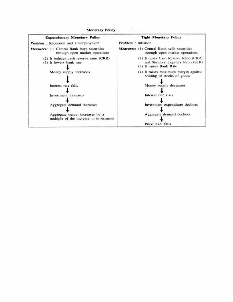
1. Expansion (Boom, Upswing or Prosperity)

2. Peak (upper turning point)

3. Contraction (Downswing, Recession or Depression)

4. Trough (lower turning point)

The four phases of business cycles have been shown in Fig. 27.1 where we start from trough

or depression when the level of economic activity i.e., level of production and employment

is at the lowest level. With the revival of economic activity the economy moves into the

expansion phase, but due to the causes explained below, the expansion cannot continue

indefinitely, and after reaching peak, contraction or downswing starts. When the

contraction gathers momentum, we have a depression.

The downswing continues till the lowest turning point which is also called trough is

reached. In this way cycle is complete. However, after remaining at the trough for some

time the economy revives and again the new cycle starts.

Four phases of business cycles:

(1) Upswing,

(2) Upper turning point,

(3) Downswing, and

(4) Lower turning point.

There are two types of patterns of cyclic changes. One pattern is shown in Fig. 27.1 where

fluctuations occur around a stable equilibrium position as shown by the horizontal line. It

is a case of dynamic stability which depicts change but without growth or trend.

The second pattern of cyclical fluctuations is shown in Fig. 27.2 where cyclical changes in

economic activity take place around a growth path (i.e., rising trend). J.R. Hicks in his

model of business cycles explains such a pattern of fluctuations with long-run rising trend

in economic activity by imposing factors such as autonomous investment due to population

growth and technological progress causing economic growth on the otherwise stationary

state. We briefly explain below various phases of business cycles.

Expansion and Prosperity:

In its expansion phase, both output and employment increase till we have full-employment

of resources and production is at the highest possible level with the given productive

resources. There is no involuntary unemployment and whatever unemployment prevails is

only of frictional and structural types.

Thus, when expansion gathers momentum and we have prosperity, the gap between

potential GNP and actual GNP is zero, that is, the level of production is at the maximum

production level. A good amount of net investment is occurring and demand for durable

consumer goods is also high. Prices also generally rise during the expansion phase but due

to high level of economic activity people enjoy a high standard of living.

Then something may occur, whether banks start reducing credit or profit expectations

change adversely and businessmen become pessimistic about future state of the economy

that bring an end to the expansion or prosperity phase.

As shall be explained below, economists differ regarding the possible causes of the end of

prosperity and start of downswing in economic activity. Monetarists have argued that

contraction in bank credit may cause downswing.

Keynes have argued that sudden collapse of expected rate of profit (which he calls marginal

efficiency of capital, MEC) caused by adverse changes in expectations of entrepreneurs

lowers investment in the economy. This fall in investment, according to him, causes

downswing in economic activity.

Contraction and Depression:

As stated above, expansion or prosperity is followed by contraction or depression. During

contraction, not only there is a fall in GNP but also level of employment is reduced. As a

result, involuntary unemployment appears on a large scale. Investment also decreases

causing further fall in consumption of goods and services.

At times of contraction or depression prices also generally fall due to fall in aggregate

demand. A significant feature of depression phase is the fall in rate of interest. With lower

rate of interest people’s demand for money holdings increases.

There is a lot of excess capacity as industries producing capital goods and consumer goods

work much below their capacity due to lack of demand. Capital goods and durable

consumer goods industries are especially hit hard during depression. Depression, it may be

noted, occurs when there is a severe contraction or recession of economic activities. The

depression of 1929-33 is still remembered because of its great intensity which caused a lot

of human suffering.

Trough and Revival:

There is a limit to which level of economic activity can fall. The lowest level of economic

activity, generally called trough, lasts for some time. Capital stock is allowed to depreciate

without replacement. The progress in technology makes the existing capital stock obsolete.

If the banking system starts expanding credit or there is a spurt in investment activity due

to the emergence of scarcity of capital as a result of non-replacement of depreciated capital

and also because of new technology coming into existence requiring new types of marines

and other capital goods. The stimulation of investment brings about the revival or recovery

of the economy.

The recovery is the turning point from depression into expansion. As investment rises, this

causes induced increase in consumption. As a result industries start producing more and

excess capacity is now put into full use due to the revival of aggregate demand.

Employment of labour increases and rate of unemployment falls. With this the cycle is

complete.

Features of Business Cycles:

Though different business cycles differ in duration and intensity they have some

common features which we explain below:

1. Business cycles occur periodically. Though they do not show same regularity, they have

.some distinct phases such as expansion, peak, contraction or depression and trough.

Further the duration of cycles varies a good deal from minimum of two years to a maximum

of ten to twelve years.

2. Secondly, business cycles are Synchronic. That is, they do not cause changes in any

single industry or sector but are of all embracing character. For example, depression or

contraction occurs simultaneously in all industries or sectors of the economy. Recession

passes from one industry to another and chain reaction continues till the whole economy is

in the grip of recession. Similar process is at work in the expansion phase, prosperity

spreads through various linkages of input-output relations or demand relations between

various industries, and sectors.

3. Thirdly, it has been observed that fluctuations occur not only in level of production but

also simultaneously in other variables such as employment, investment, consumption, rate

of interest and price level.

4. Another important feature of business cycles is that investment and consumption of

durable consumer goods such as cars, houses, refrigerators are affected most by the cyclical

fluctuations. As stressed by J.M. Keynes, investment is greatly volatile and unstable as it

depends on profit expectations of private entrepreneurs. These expectations of

entrepreneurs change quite often making investment quite unstable. Since consumption of

durable consumer goods can be deferred, it also fluctuates greatly during the course of

business cycles.

5. An important feature of business cycles is that consumption of non-durable goods and

services does not vary much during different phases of business cycles. Past data of

business cycles reveal that households maintain a great stability in consumption of non-

durable goods.

6. The immediate impact of depression and expansion is on the inventories of goods. When

depression sets in, the inventories start accumulating beyond the desired level. This leads

to cut in production of goods. On the contrary, when recovery starts, the inventories go

below the desired level. This encourages businessmen to place more orders for goods

whose production picks up and stimulates investment in capital goods.

7. Another important feature of business cycles is profits fluctuate more than any other type

of income. The occurrence of business cycles causes a lot of uncertainty for businessmen

and makes it difficult to forecast the economic conditions. During the depression period

profits may even become negative and many businesses go bankrupt. In a free market

economy profits are justified on the ground that they are necessary payments if the

entrepreneurs are to be induced to bear uncertainty.

8. Lastly, business cycles are international in character. That is, once started in one country

they spread to other countries through trade relations between them. For example, if there

is a recession in the USA, which is a large importer of goods from other countries, will

cause a fall in demand for imports from other countries whose exports would be adversely

affected causing recession in them too. Depression of 1930s in USA and Great Britain

engulfed the entire capital world.

Theories of Business Cycles

Some of the most important theories of business cycles are as follows:

1. Pure Monetary Theory 2. Monetary Over-Investment Theory 3. Schumpeter’s Theory of

Innovation 4. Keynes Theory 5. Samuelson’s Model of Multiplier Accelerator Interaction

6. Hicks’s Theory.

A number of theories have been developed by different economists from time to time to

understand the concept of business cycles. In the first half of twentieth century, various

new and important concepts related to business cycles come into existence.

However, in nineteenth century, many of the classical economists, such as Adam Smith,

Miller, and Ricardo, have conducted a study on business cycles. They linked economic

activities with the Say’s law, which states that supply creates its own demand. They

believed that stability of an economy depends on market forces. After that, many other

economists, such as Keynes and Hick, had provided a framework to understand business

cycles.

1. Pure Monetary Theory:

The traditional business cycle theorists take into consideration the monetary and credit

system of an economy to analyze business cycles. Therefore, theories developed by these

traditional theorists are called monetary theory of business cycle. The monetary theory

states that the business cycle is a result of changes in monetary and credit market

conditions. Hawtrey, the main supporter of this theory, advocated that business cycles are

the continuous phases of inflation and deflation. According to him, changes in an economy

take place due to changes in the flow of money. For example, when there is increase in

money supply, there would be increase in prices, profits, and total output. This results in

the growth of an economy. On the other hand, a fall in money supply would result in

decrease in prices, profit, and total output, which would lead to decline of an economy.

Apart from this, Hawtrey also advocated that the main factor that influences the flow of

money is credit mechanism. In economy, the banking system plays an important role in

increasing money flow by providing credit.

An economy shows growth when the volume of bank credit increases. This increase in the

growth continues till the volume of bank credit increases. Banks offer credit facilities to

individuals or organizations due to the fact that banks find it profitable to provide credit on

easy terms.

The easy availability of funds from banks helps organizations to perform various business

activities. This leads to increase in various investment opportunities, which further results

in deepening and widening of capital. Apart from this, credit provided by banks on easy

terms helps organizations to expand their production.

When an organization increases its production, the supply of its products also increases to

a certain limit. After that, the rate of increase in demand of products in market is higher

than the rate of increase in supply. Consequently, the prices of products increases.

Therefore, credit expansion helps in expansion of economy. On the contrary, the economic

condition is reversed when the bank starts withdrawing credit from market or stop lending

money.

This is because of the reason that the cash reserves of bank are washed-out due to the

following reasons:

a. Increase in loans and advance provided by banks

b. Reduction in inflow of deposits

c. Withdrawal of deposits for better investment opportunities

When banks stop providing credit, it reduces investment by businessmen. This leads to the

decrease in the demand for consumer and capital goods, prices, and consumption. This

marks the symptoms of recession.

Some of the points on which the pure monetary theory is criticized are as follows:

a. Regards business cycle as monetary phenomenon that is not true. Apart from monetary

factors, several non-monetary factors, such as new investment demands, cost structure, and

expectations of businessmen, can also produce changes in economic activities.

b. Describes only expansion and recession phases and fails to explain the intermediary

phases of business cycles.

c. Assumes that businessmen are more sensitive to the interest rates that is not true rather

they are more concerned about the future opportunities.

2. Monetary Over-Investment Theory:

Monetary over-investment theory focuses mainly on the imbalance between actual and

desired investments. According to this theory, the actual investment is much higher than

the desired investment. This theory was given by Hayek.

According to him, the investment and consumption patterns of an economy should match

with each other to bring the economy in equilibrium. For stabilizing this equilibrium, the

voluntary savings should be equal to actual investment in an economy.

In an economy, generally, the total investment is distributed among industries in such a

way that each industry produces products to a limit, so that its demand and supply are

equal. This implies that the investment at every level and for every product in the whole

economy is equal. As a result, there would be no expansion and contraction and the

economy would always be in equilibrium.

According to this theory, changes in economic conditions would occur only when the

money supply and investment-saving relations show fluctuations. The investment-saving

relations are affected when there is an increase in investment opportunities and voluntary

savings are constant.

Investment opportunities increase due to several reasons, such as low interest rates,

increased marginal efficiency of capital, and increase in expectations of businessmen.

Apart from this, when banks start supporting industries for investment by lending money

at lower rates, it results in an increase in investment.

This may result in the condition of overinvestment mainly in capital good industries. In

such a case, investment and savings increase, but the consumption remains unaffected as

there is no change in consumer goods industries.

Consequently, profit increases with increase in investment opportunities, which further

results in an increase in the demand for various products and services. The demand for

products and services exceeds the supply of products and services.

This leads to inflation in the economy, which reduces the purchasing power of individuals.

Therefore, with decrease in the purchasing power of individuals, the real demand for

products does not increase at the same rate at which the investment increases. The real

investment is done at the cost of real consumption.

The balance between the investment and consumer demand is disturbed. As a result, it is

difficult to maintain the current rate of investment. The demand of consumer goods would

be dependent on the income of individuals.

An increase in the income level would result in the increase of consumer goods. However,

the increase in consumer goods is more than the increase in capital goods. Therefore,

people would invest in consumer goods rather than in capital goods. Consequently, the

demand for bank credit also increases.

However, the bankers are not ready to lend money because of the demand for funds from

consumer and capital goods industry both. This leads to recession in the economy. As a

result, economic activities, such as employment, investment, savings, consumption, and

prices of goods and services, start declining.

Some of the limitations of monetary over-investment theory are as follows:

a. Assumes that when the market rate of interest is lower than the natural market rate of

interest, the bank credit flows to the capital goods industry. This is applicable only in the

situation of full employment. However, business cycles are the part of an economy and can

take place under improper utilization of resources.

b. Considers interest rate as the most important factor that affects investment. However,

there are several factors, such as capital goods cost and businessmen expectations, which

can influence investment.

c. Focuses on balance between consumer goods and investment, which is not much

required.

3. Schumpeter’s Theory of Innovation:

The other theories of business cycles lay emphasis on investment and monetary expansion.

The Schumpeter’s theory of innovation advocates that business innovations are responsible

for rapid changes in investment and business fluctuations.

According to Schumpeter said, “Business cycles are almost exclusively the result of

innovations in the industrial and commercial organization. Innovations are such changes

of the combination of the factors of production as cannot be effected by infinitesimal steps

or variations on the margin. [Innovation] consists primarily in changes in methods of

production and transportation, or changes in industrial organization, or in the production

of a new article, or opening of a new market or of new sources of material.”

According to Schumpeter, innovation refers to an application of a new technique of

production or new machinery or a new concept to reduce cost and increase profit. In

addition, he propounded that innovations are responsible for the occurrence of business

cycles. He also designed a model having two stages, namely, first approximation and

second approximation.

The two stages of the model are discussed as follows:

(a) First Approximation:

Deals with the effect of innovatory ideas on an economy in the beginning. First

approximation is the startup stage of innovation in which the economy is in equilibrium.

This implies when Marginal Cost (MC) is equal to Marginal Revenue (MR) and Average

Cost (AC) is equal to price. In addition, at this stage, there is no involuntary unemployment.

In equilibrium, organizations lack idle funds or surplus funds to invest. In such a case,

banks are the only source of funds for innovators. When the innovators get the desired fund

from banks, they purchase inputs for production at a higher price to make these inputs

available only for innovation purposes.

Increase in prices of inputs result in the rise of prices. Over time, competitors also start

copying innovation and acquire funds from bank. As a result, the output and profit of

organizations start increasing.

However, after a certain point of time, profit shows decline with a decrease in output prices.

Simultaneously, debtors need to repay their debts to bank. This leads to decrease in the

flow of money, which finally results in recession.

(b) Second Approximation:

Deals with the subsequent effects of first approximation. It is related to the speculation of

future economic conditions. In first approximation, it is assumed by investors that the

expansion phase would not be affected in future, especially in capital goods industries. On

the basis of this belief, investors take large amounts of money from banks.

In addition, in this stage, customers perceive an increase in the durable goods in future and

therefore, start purchasing goods at present by borrowing funds. When the prices start

falling, debtors are in the worst situation because they are not able to repay loan and meet

their basic needs. This leads to depression in the economy.

4. Keynes Theory:

Keynes theory was developed in 1930s, which was the period when whole world was going

through great depression. This theory is the reply of Keynes to classical economists.

According to classical economists, if there is high unemployment condition in an economy,

then economic forces, such as demand and supply, would act in a manner to bring back full

employment condition.

In his theory of business cycles, Keynes advocated that the total demand helps in the

determination of various economic factors, such as income, employment, and output. The

total demand refers to the demand of consumer and capital goods.

In such a case, total investment and expenditure on products and services is more, the level

of production would increase. When the level of production increases, it results in the

increase of employment opportunities and income level. However, if the total demand is

low, the level of production would also be less.

Consequently, the income, output and investment would also be low. Therefore, changes

in income and output level are produced by changes in total demand. The total demand is

further affected by changes in the demand of investment, which depends on the rate of

interest and expected rate of profit.

Keynes referred expected rate of profit as the marginal efficiency of capital. Expected rate

of profit is the difference between the expected revenue generated by the capital employed

and the cost incurred to employ that capital.

In case, the expected rate of profit is greater than the current rate of interest, then the

investors would invest more. On the other hand, the marginal efficiency of capital is

determined by expected return from capital goods and cost involved in the replacement of

capital goods.

Marginal efficiency of a capital increases due to new inventions or innovations in economic

factors, such as product, production technique, investment option, assuming that prices

would rise in future. On the other hand, it decreases due to various reasons, such as decrease

in prices, increase in costs, and inefficiency of the production process.

According to Keynes theory, in the expansion phase of business cycle, investors are

positive about economic conditions, thus, they overestimate the rate of return from an

investment. The rate of return increases until the full employment condition is not achieved.

When the economy is on the path of achieving full employment, this phase is termed as

boom phase. In the boom phase, investors are not able to diagnose the fall in marginal

efficiency of capital and even do not consider the rate of interest. As a result, the profit

from investments starts Calling due to the increase in the cost of investment and production

of goods and services. This situation results in the contraction or recession in economy.

This is because the rate of decrease in the marginal efficiency of capital is more than that

of current rate of interest. In addition, in this situation, investment opportunities shrink.

Banks are not also able to provide credit because of the lack of funds.

Current rate of interest is higher that encourages people to save rather than invest. As a

result, the demand for consumer and capital goods decreases. Further, the income and

employment level decreases and economy reaches to the phase of depression.

Keynes has proposed three types of propensities to understand business cycles. These are

propensity to save, propensity to consume, and propensity of marginal efficiency of capital.

He has also developed a concept of multiplier that represents changes in income level

produced by the changes in investment.

Keynes also advocated that the expansion of business cycle occurs due to increase in

marginal efficiency of capital. This encourages investors (including individuals and

organizations) to invest. Organizations replace their capital goods and start production.

As a result, the income of individuals increases, which further increases the rate of

consumption. This increases the profit of organizations, which finally lead to an increase

in the total income and investment level of an economy. This marks the recovery phase of

an economy.

Some points of criticism of Keynes theory are as follows:

a. Fails to explain the recurrence of business cycles.

b. Ignores the accelerator’s role to describe business cycles. However, a business cycle can

be explained property with the help of multiplier acceleration interaction.

c. Offers only a systematic framework for business cycles, not the whole concept.

5. Samuelson’s Model of Multiplier Accelerator Interaction:

The economists of post-Keynesian period emphasized the need of both multiplier and

accelerator concepts to explain business cycles. Samuelson’s model of multiplier

accelerator interaction was the first model that represents interaction between these two

concepts.

In his model, Samuelson has described the way the multiplier and accelerator interact with

each other for generating income and increasing consumption and demand of investment.

He also describes how these two factors are responsible for creating economic fluctuations.

Samuelson used two concepts, namely, autonomous and derived investment, to explain his

model. Autonomous investment refers to the investment due to exogenous factors, such as

new product, production technique, and market.

On the other hand, derived investment refers to the increase in the investment of capital

goods produced due to increase in the demand of consumer goods. When autonomous

investment occurs in an economy, the income level also increases.

This brought the role of multiplier into account. The income level helps in determining the

marginal propensity to consume. If the income level increases, then the demand for

consumer goods also increases.

The supply of consumer goods should satisfy the demand for consumer goods. This is

possible when the production technique is capable to produce a large quantity of products

and services. This encourages organizations to invest more to develop advanced production

techniques and increase production for meeting consumer demand.

Therefore, the consumption affects the demand of investment. This is referred as derived

investment. This marks the starting of the acceleration process, which results in further

increase in income level.

An increase in the income level would increase the demand of consumer goods. In this

manner, the multiplier and accelerator interact with each other and make the income grow

at a much higher rate than expected.

Autonomous investment leads to multiplier effect that result in derived investment. This is

called acceleration of investment. Derived investment would make the accelerator to come

into action. This is termed as multiplier-acceleration interaction.

Samuelson made certain assumptions for the explanation of business cycles. Some of the

assumptions are that the production capacity is limited and consumption takes place after

a gap of one year.

Another assumption made by him is that there would be a gap of one year between the

increase in consumption and increase in the demand of investment. In addition, he assumed

that there would be no government activity and foreign trade in the economy.

According to the assumption given by Samuelson that there would be no government

activity and foreign trade, the equilibrium would be achieved when

Yt = Ct + It

Where, Yt = National income

Ct = Total consumption expenditure

It = Investment expenditure

t = Time period

According to the assumption that consumption takes place after a gap of one year,

the consumption function would be represented as follows:

Ct = α Yt-1

Where, Yt-1 = Income for t-1 time period

α = ∆C/∆Y (multiplier propensity to consume)

Investment and consumption has a time lag of one year; therefore, the investment

function can be expressed a follows:

It = b (Ct –Ct-1)

Where, b = capital/output ratio (helps in determination of acceleration)

By putting the value of Ct and It in the first equation of national income, we get

Yt = α Yt-1 + b (Ct – Ct-1)

If Ct = α Yt-1, then Ct-1 = α Yt-2. Putting the value of Ct-1 in the preceding equation, we get

Yt = α Yt-1 + b (α Yt-1 -α Yt-2)

Yt = α (1 + b) Yt-1 – abYt-2 (equation for equilibrium)

With the help of preceding equation, the income level for past and future can be determined

if the values of a, b and income of two preceding years are given. It can be depicted from

the preceding equation that the changes in income level can be affected by the values of α

and b.

The different combinations of α and b give rise to fluctuations in business cycles as

shown in Figure-4:

In Figure-4, the areas A, B, C, and D represents the different phases of business cycles.

The types of different cycles represented by A, B, C, and D are described in detail with the

help of the following points:

A: Refers to the area at which the income level increases or decreases at the decreasing

rate and arrive at a new equilibrium point. The change in the income level would be in one-

direction only.

It results in damped non-oscillation, as shown in Figure-5:

B: Refers to the area in which points, a and b, together makes amplitude cycles that

gradually become smaller. This process continues till the cycles get dissolve and economy

reaches to equilibrium.

This represents damped oscillations, as shown in Figure-6:

C: Refers to the area in which points, a and b, together makes amplitude cycles that become

larger.

This forms explosive cycles, as shown in Figure-7:

D: Refers to the area at which the income level is increasing or decreasing at the

exponential rate. This process continues till cycles reach at the bottom.

It represents one-way explosion and results in explosive oscillations, as shown in

Figure-8:

E: Refers to the point at which the oscillations are of equal amplitude.

Some of the drawbacks of Samuelson’s model are as follows:

a. Represents a simpler model that is not able to explain business cycles completely

b. Ignores other factors that influence business cycles, such as expectations of businessmen

and taste and preferences of customers

c. Assumes that the capital/output ratio remains constant, which is not true.

6. Hicks’s Theory:

Hicks has associated business cycles to the growth theory of Harrod-Domar. According to

him, business cycles take place simultaneously with economic growth; therefore, business

cycles should be explained in association with the growth theory.

In his theory, he has used the following concepts to explain business cycles:

a. Saving-investment relation and multiplier concepts given by Keynes

b. Acceleration concept given by Clark

c. Multiplier-acceleration interaction concepts given by Samuelson

d. Growth model of Harrod-Domar

Hicks has also framed certain assumptions for describing business cycle concept.

The important assumptions of Hicks’s theory are as follows:

(a) Assumes an equilibrium rate of growth in a model economy where realized growth rate

(Gr) and natural growth rate (Gn) are equal. As a result, the increase in autonomous

investment is constant and is equal to the increase in voluntary savings. The equilibrium

growth rate can be obtained with the help of rate of autonomous investment and voluntary

savings.

(b) Assumes the consumption function given by Samuelson, which is Ct = α Yt-1. As

discussed earlier, according to Samuelson theory consumption takes place after a lag of

one year. The time lag in consumption occurs due to the gap between income and

expenditure and gap between Gross National Product (GNP) and non-wage income.

The gap between income and expenditure produces when income is ahead of expenditure.

The gap between GNP and non-wage income produces when fluctuations in GNP occur

more frequently than the fluctuations in non-wage income.

The saving function becomes the function of past year’s income. With the time lag between

income and investment-saving, the multiplier process has a diminishing impact on business

cycles.

(c) Assumes that autonomous investment is a function of output at present. In addition,

autonomous investment is used for replacing capital goods. However, induced investment

is regarded as the function of changes in output.

The change in output produces induced investment, which marks the beginning of the

acceleration process. The acceleration process interrelates with the multiplier effect on

income and consumption.

(d) Makes use of the words ceiling and bottom for explaining the upward and downward

flow of business cycles. The ceiling on upward flow is a result of scarcity of resources

required. On the other hand, the bottom on downward flow does not have a direct limit on

contraction. However, an indirect limit is the effect of accelerator on depression.

Hicks’s theory can be explained with the help of Figure-9:

In Figure-9, the y-axis represents the logarithms of output and employment while x-axis

represents the semi-logarithm of time AA line represents the autonomous investment that

is rising at the same rate.

EE line shows the equilibrium line that is a multiple of autonomous investment. FF line

expresses the full employment or the peak phase of economy, while LL line expresses the

trough phase of an economy.

Hicks explains business cycles by assuming that the economy has reached to Po point of

equilibrium path and autonomous investment is the result of innovation. The autonomous

investment results in the increase of output.

Consequently, the economy moves upward from the equilibrium path. After a certain point

of time, the autonomous investment brings the multiplier process at work, which further

increases output and employment. The increased output makes the induced investment to

work that further results in accelerator process to work.

The multiplier-accelerator interaction results in the growth of the economy. Consequently,

the economy enters in the phase of expansion. The economy moves on the expansion path

of P0P1. At point P1, the economy is in full employment condition. Now, the economy

cannot grow further, it can only move on the FF line.

However, it cannot remain at FF line because autonomous investment becomes constant;

therefore, now at FF, only the normal autonomous investment would be produced. This

infers that the expansion of the economy is governed by induced investment only.

When the economy reaches to point P1, the increase in induced investment becomes stable

and the growth of economy starts declining. This is because of the reason that the output

produced at FF line is not sufficient for induced investment.

As a result the induced investment stops. The decline of the economy can be postponed, if

the time lag between output and investment is of three to four years. However, the decline

in output cannot be ceased. When the decline in output occurs at point P then the decline

in output would continue till the economy reaches back to EE line.

After arriving at EE line, it would continue to fall further. The rate of decline in economy

is very slow because disinvestment depends on the rate of depreciation. The decrease in

output leads to the decline in the rate of depreciation.

The effect of reverse accelerator on the depression is not as frequent as in the case of

expansion. During the path Q1Q2, the induced investment is nil while autonomous

investment is less than normal. In addition, the indefinite decline of economy is represented

by Q1q. However, Q1q is a very rare case that does not occur normally.

When the economy reaches to trough, it moves along the LL line, which is associated with

AA line that represents autonomous investment. Therefore, output starts increasing again

with the increase in autonomous investment.

Increase in output makes the accelerator to work again. This phase is termed as recovery

phase. Along with accelerator, multiplier also comes into action and their interaction makes

economy run on the growth path and reaches to equilibrium EE line again.

There are certain limitations of Hicks’s theory, which are as follows:

a. Fails to explain the reasons for linear consumption function and constant multiplier.

When the economy is going through different phases of business cycles, the income is

redistributed that affects the marginal propensity to consume, which further affects the

multiplier process.

b. Suspects the constancy of multiplier in changing economic conditions. Without practical

evidence, the accelerator and multiplier cannot be assumed to be constant.

c. Takes into consideration the abstract theory, which cannot be applied in the real world.

Theories of Demand for Money

1 Fisher’s Transactions Approach to Demand for Money

In his theory of demand for money Fisher and other classical economists laid stress on the medium

of exchange function of money, that is, money as a means of buying goods and services. All

transactions involving purchase of goods, services, raw materials, assets require payment of money

as value of the transaction made.

If accounting identity, namely value paid must equal value received is to occur, value of goods,

services and assets sold must be equal to the value of money paid for them. Thus, in any given

period, the value of all goods, services or assets sold must equal to the number of transactions

made multiplied by the average price of these transactions. Thus, the total value of transactions

made is equal to PT.

On the other hand, because value paid is identically equal to the value of money flow used for

buying goods, services and assets, the value of money flow is equal to the nominal quantity of

money supply M multiplied by the average number of times the quantity of money in circulation

is used or exchanged for transaction purposes. The average number of times a unit of money is

used for transactions of goods, services and assets is called transactions velocity of circulation and

is denoted by V.

Symbolically, Fisher’s equation of exchange is written as under:

MV = PT …(1)

Where, M = the quantity of money in circulation

V = transactions velocity of circulation

P = Average price

T = the total number of transactions.

The above equation (1) is an identity that is true by definition. However by taking some

assumptions about the variables V and T, Fisher transformed the above identity into a theory of

demand for money.

According to Fisher, the nominal quantity of money M is fixed by the Central Bank of a country

(note that Reserve Bank of India is the Central Bank of India) and is therefore treated as an

exogenous variable which is assumed to be a given quantity in a particular period of time.

Further, the number of transactions in a period is a function of national income; the greater the

national income, the larger the number of transactions required to be made. Further, since Fisher

assumed that full employment of resources prevailed in the economy, the level of national income

is determined by the amount of the fully employed resources.

Thus, with the assumption of full employment of resources, the volume of transactions T is fixed

in the short run. But most important assumption which makes Fisher’s equation of exchange as a

theory of demand for money is that velocity of circulation (V) remains constant and is independent

of M, P and T.

This is because he thought that velocity of circulation of money (V) is determined by institutional

and technological factors involved in the transactions process. Since these institutional and

technological factors do not vary much in the short run, the transactions velocity of circulation of

money (V) was assumed to be constant.

As we know that for money market to be in equilibrium, nominal quantity of money supply must

be equal to the nominal quantity of money demand.

In other words, for money market to be in equilibrium:

Ms = Md

where Ms is fixed by the Central Bank of a country.

With the above assumptions, Fisher’s equation of exchange in (1) above can be rewritten as

Md = PT/V

or Md = 1/V. PT …(2)

Thus, according to Fisher’s transactions approach, demand for money depends on the

following three factors:

(1) The number of transactions (T)

(2) The average price of transactions (P)

(3) The transaction velocity of circulation of money

It has been pointed out that Fisher’s transactions approach represents some kind of a mechanical

relation between demand for money (Md) and the total value of transactions (PT). Thus in Fisher’s

approach the relation between demand for money Md and the value of transactions (PT) “portrays

some kind of a mechanical relation between it (i.e. PT) and Md as PT represents the total amount

of work to be done by money as a medium of exchange. This makes demand for money (Md) a

technical requirement and not a behavioural function”.

In Fisher’s transactions approach to demand for money some serious problems are faced when it

is used for empirical research. First, in Fisher’s transactions approach, not only transactions

involving current production of goods and services are included but also those which arise in sales

and purchase of capital assets such as securities, shares, land etc. Due to frequent changes in the

values of these capital assets, it is not appropriate to assume that T will remain constant even if Y

is taken to be constant due to full-employment assumption.

The second problem which is faced in Fisher’s approach is that it is difficult to define and

determine a general price level that covers not only goods and services currently produced but also

capital assets just mentioned above.

2 The Cambridge Cash Balance Theory of Demand for Money

Cambridge Cash Balance theory of demand for money was put forward by Cambridge economists,

Marshall and Pigou. This Cash Balance theory of demand for money differs from Fisher’s

transactions approach in that it places emphasis on the function of money as a store of value or

wealth instead of Fisher’s emphasis on the use of money as a medium of exchange.

It is worth noting that the exchange function of money eliminates the need to barter and solves the

problem of double coincidence of wants faced in the barter system. On the other hand, the function

of money as a store of value lays stress on holding money as a general purchasing power by

individuals over a period of time between the sale of a goods or service and subsequent purchase

of a good or service at a later date.

Marshall and Pigou focused their analysis on the factors that determine individual demand for

holding cash balances. Although they recognized that current interest rate, wealth owned by the

individuals, expectations of future prices and future rate of interest determine the demand for

money, they however believed that changes in these factors remain constant or they are

proportional to changes in individuals’ income.

Thus, they put forward a view that individual’s demand for cash balances (i.e. nominal money

balances) is proportional to the nominal income (i.e. money income).

Thus, according to their approach, aggregate demand for money can be expressed as:

Md = kPY

Where, Y = real national income

P = average price level of currently produced goods and services

PY = nominal income

k = proportion of nominal income (PY) that people want to hold as cash balances

Cambridge Cash balance approach to demand for money is illustrated in Fig. 15.1 where on the

X-axis we measure nominal national income (PY) and on the F-axis the demand for money (Md).

It will be seen from Fig. 15.1 that demand for money (Md) in this Cambridge Cash Balance

Approach is a linear function of nominal income. The slope of the function is equal to k, that is,

k = Md/Py .Thus important feature of Cash balance approach is that it makes the demand for money

as function of money income alone.

A merit of this formulation is that it makes the relation between demand for money and income as

behavioral in sharp contrast to Fisher’s approach in which demand for money was related to total

transactions in a mechanical manner.

Although, Cambridge economists recognized the role of other factors such as rate of interest,

wealth as the factors which play a part in the determination of demand for money but these factors

were not systematically and formally incorporated into their analysis of demand for money.

In their approach, these other factors determine the proportionality factor k, that is, the proportion

of money income that people want to hold in the form of money, i.e. cash balances. It was J.M.

Keynes who later emphasized the role of these other factors such as rate of interest, expectations

regarding future interest rate and prices and formally incorporated them explicitly in his analysis

of demand for money.

“Cambridge approach is conceptually richer than the transactions approach, the former is

incomplete because it does not formally incorporate the influence of economic variables just

mentioned on the demand for cash balances… John Maynard Keynes first attempted to eliminate

this shortcoming.”

Another important feature of Cambridge demand for money function is that the demand for money

is proportional function of nominal income (Md= kPY). Thus, it is proportional function of both

price level (P) and real income (Y). This implies two things. First, income elasticity of demand for

money is unity and, secondly, price elasticity of demand for money is also equal to unity so that

any change in the price level causes equal proportionate change in the demand for money.

Criticism:

It has been pointed out by critics that other influences such as rate of interest, wealth, expectations

regarding future prices have not been formally introduced into the Cambridge theory of the

demand for cash balances. These other influences remain in the background of the theory. “It was

left to Keynes, another Cambridge economist, to highlight the influence of the rate of interest on

the demand for money and change the course of monetary theory.”

Another criticism leveled against this theory is that income elasticity of demand for money may

well be different from unity. Cambridge economists did not provide any theoretical reason for its

being equal to unity. Nor is there any empirical evidence supporting unitary income elasticity of

demand for money.

Besides, price elasticity of demand is also not necessarily equal to unity. In fact, changes in the

price level may cause non-proportional changes in the demand for money. However, these

criticisms are against the mathematical formulation of cash balance approach, namely, Md = kPY.

They do not deny the important relation between demand for money and the level of income.

Empirical studies conducted so far point to a strong evidence that there is a significant and firm

relation between demand for money and level of income.

3 Keynes’ Theory of Demand for Money

In his well-known book, Keynes propounded a theory of demand for money which occupies an

important place in his monetary theory. It is also worth noting that for demand for money to hold

Keynes used the term what he called liquidity preference. How much of his income or resources

will a person hold in the form of ready money (cash or non-interest-paying bank deposits) and how

much will he part with or lend depends upon what Keynes calls his “liquidity preference.”

Liquidity preference means the demand for money to hold or the desire of the public to hold cash.

Demand for Money or Motives for Liquidity Preference: Keynes’ Theory:

Liquidity preference of a particular individual depends upon several considerations. The question

is: Why should the people hold their resources liquid or in the form of ready money when they can

get interest by lending money or buying bonds?

The desire for liquidity arises because of three motives:

(i) The transactions motive,

(ii) The precautionary motive, and

(iii) The speculative motive.

1. The Transactions Demand for Money:

The transactions motive relates to the demand for money or the need for money balances for the

current transactions of individuals and business firms. Individuals hold cash in order “to bridge

the interval between the receipt of income and its expenditure”. In other words, people hold money

or cash balances for transaction purposes, because receipt of money and payments do not coincide.

Most of the people receive their incomes weekly or monthly while the expenditure goes on day by

day. A certain amount of ready money, therefore, is kept in hand to make current payments. This

amount will depend upon the size of the individual’s income, the interval at which the income is

received and the methods of payments prevailing in the society.

The businessmen and the entrepreneurs also have to keep a proportion of their resources in money

form in order to meet daily needs of various kinds. They need money all the time in order to pay

for raw materials and transport, to pay wages and salaries and to meet all other current expenses

incurred by any business firm.

It is clear that the amount of money held under this business motive will depend to a very large

extent on the turnover (i.e., the volume of trade of the firm in question). The larger the turnover,

the larger, in general, will be the amount of money needed to cover current expenses. It is worth

noting that money demand for transactions motive arises primarily because of the use of money as

a medium of exchange (i.e. means of payment).

Since the transactions demand for money arises because individuals have to incur expenditure on

goods and services during the receipt of income and its use of payment for goods and services,

money held for this motive depends upon the level of income of an individual.

A poor man will hold less money for transactions motive as he spends less because of his small

income. On the other hand, a rich man will tend to hold more money for transactions motive as his

expenditure will be relatively greater

The demand for money is a demand for real cash balances because people hold money for the

purpose of buying goods and services. The higher the price level, the more money balances a

person has to hold in order to purchase a given quantity of goods. If the price level doubles, then

the individual has to keep twice the amount of money balances in order to be able to buy the same

quantity of goods. Thus the demand for money balances is demand for real rather than nominal

balances.

According to Keynes, the transactions demand for money depends only on the real income and is

not influenced by the rate of interest. However, in recent years, it has been observed empirically

and also according to the theories of Tobin and Baumol transactions demand for money also

depends on the rate of interest.

This can be explained in terms of opportunity cost of money holdings. Holding one’s asset in the

form of money balances has an opportunity cost. The cost of holding money balances is the interest

that is foregone by holding money balances rather than other assets. The higher the interest rate,

the greater the opportunity cost of holding money rather than non-money assets.

Individuals and business firms economies on their holding of money balances by carefully

managing their money balances through transfer of money into bonds or short-term income

yielding non-money assets. Thus, at higher interest rates, individuals and business firms will keep

less money holdings at each level of income.

2. Precautionary Demand for Money:

Precautionary motive for holding money refers to the desire of the people to hold cash balances

for unforeseen contingencies. People hold a certain amount of money to provide for the danger of

unemployment, sickness, accidents, and the other uncertain perils. The amount of money

demanded for this motive will depend on the psychology of the individual and the conditions in

which he lives.

3. Speculative Demand for Money:

The speculative motive of the people relates to the desire to hold one’s resources in liquid form in

order to take advantage of market movements regarding the future changes in the rate of interest

(or bond prices). The notion of holding money for speculative motive was a new and revolutionary

Keynesian idea. Money held under the speculative motive serves as a store of value as money held

under the precautionary motive does. But it is a store of money meant for a different purpose.

The cash held under this motive is used to make speculative gains by dealing in bonds whose prices

fluctuate. If bond prices are expected to rise which, in other words, means that the rate of interest

is expected to fall, businessmen will buy bonds to sell when their prices actually rise. If, however,

bond prices are expected to fall, i.e., the rate of interest is expected to rise, businessmen will sell

bonds to avoid capital losses.

Nothing is certain in the dynamic world, where guesses about the future course of events are made

on precarious basis, businessmen keep cash to speculate on the probable future changes in bond

prices (or the rate of interest) with a view to making profits.

Given the expectations about the changes in the rate of interest in future, less money will be held

under the speculative motive at a higher current rate of interest and more money will be held under

this motive at a lower current rate of interest.

The reason for this inverse correlation between money held for speculative motive and the

prevailing rate of interest is that at a lower rate of interest less is lost by not lending money or

investing it, that is, by holding on to money, while at a higher current rate of interest holders of

cash balance would lose more by not lending or investing.

Thus the demand for money under speculative motive is a function of the current rate of interest,

increasing as the interest rate falls and decreasing as the interest rate rises. Thus, demand for money

under this motive is a decreasing function of the rate of interest. This is shown in Fig. 15.2. Along

X-axis we represent the speculative demand for money and along the y-axis the current rate of

interest.

The liquidity preference curve LP is downward sloping towards the right signifying that the higher

the rate of interest, the lower the demand for money for speculative

motive, and vice versa. Thus at the high current rate of interest Or, a very small amount OM is

held for speculative motive.

This is because at a high current rate of interest more money would have been lent out or used for

buying bonds and therefore less money would be kept as inactive balances. If the rate of interest

falls to Or’, then a greater amount of money OM is held under speculative motive. With the further

fall in the rate -of interest to Or’, money held under speculative motive increases to OM.

Liquidity Trap

It can be seen from Fig. that the liquidity preference curve LP becomes quite flat i.e., perfectly

elastic at a very low rate of interest; it is horizontal line beyond point E” towards the right. This

perfectly elastic portion of liquidity preference curve indicates the position of absolute liquidity

preference of the people. That is, at a very low rate of interest people will hold with them as inactive

balances any amount of money they come to have.

This portion of liquidity preference curve with absolute liquidity preference is called liquidity trap

by the economists because expansion in money supply gets trapped in the sphere of liquidity trap

and therefore cannot affect rate of interest and therefore the level of investment. According to

Keynes, it is because of the existence of liquidity trap that monetary policy becomes ineffective to

tide over economic depression.

But the demand for money to satisfy the speculative motive does not depend so much upon what

the current rate of interest is, as on expectations about changes in the rate of interest. If there is a

change in the expectations regarding the future rate of interest, the whole curve of demand for

money or liquidity preference for speculative motive will change accordingly.

Thus, if the public on balance expect the rate of interest to be higher (i.e., bond prices to be lower)

in the future than had been previously supposed, the speculative demand for money will increase

and the whole liquidity preference curve for speculative motive will shift upward.

Aggregate Demand for Money: Keynes’ View

If the total demand of money is represented by Md we may refer to that part of M held for

transactions and precautionary motive as M1 and to that part held for the speculative motive as M2.

Thus Md= M1 + M2. According to Keynes, the money held under the transactions and precautionary

motives, i.e., M1, is completely interest-inelastic unless the interest rate is very high.

The amount of money held as M1, that is, for transactions and precautionary motives, is mainly a

function of the size of income and business transactions together with the contingencies growing

out of the conduct of personal and business affairs.

We can write this in a functional form as follows:

M1 = L1(Y) …(i)

where Y stands for income, L1 for demand function, and M1 for money demanded or held under

the transactions and precautionary motives. The above function implies that money held under the

transactions and precautionary motives is a function of income.

On the other hand, according to Keynes, money demanded for speculative motive, i.e., M2 as

explained above, is primarily a function of the rate of interest.

This can be written as:

M2 = L2(r) …(ii)

Where r stands for the rate of interest, L2 for demand function for speculative motive.

Since total demand of money Md = M1 + M2, we get from (i) and (ii) above

Md = L1(Y) + L2(r)

Thus, according to Keynes’ theory of total demand for money is an additive demand function with

two separate components. The one component, L1(Y) represents the transactions demand for

money arising out of transactions and precautionary motives is an increasing function of the level

of money income. The second component of the demand for money, that is, L2(r) represents the

speculative demand for money, which depends upon rate of interest, is a decreasing function of

the rate of interest.

Critique of Keynes’ Theory

By introducing speculative demand for money, Keynes made a significant departure from the

classical theory of money demand which emphasized only the transactions demand for money.

However, as seen above, Keynes’ theory of speculative demand for money has been challenged.

The main drawback of Keynes’ speculative demand for money is that it visualizes that people hold

their assets in either all money or all bonds. This seems quite unrealistic as individuals hold their

financial wealth in some combination of both money and bonds. This gave rise to portfolio

approach to demand for money put forward by Tobin, Baumol and Friedman.

The portfolio of wealth consists of money, interest-bearing bonds, shares, physical assets etc.

Further, while according to Keynes’ theory, demand for money for transaction purposes is

insensitive to interest rate, the modern theories of money demand put forward by Baumol and

Tobin show that money held for transaction purposes is interest elastic.

Further, Keynes’ additive form of demand for money function, namely, Md= LX(Y) + L2 (r) has

now been rejected by the modem economists. It has been pointed out that money represents a

single asset, and not the several ones. There may be more than one motive to hold money but the

same units of money can serve several motives. Therefore, the demand for money cannot be

divided into two or more different departments independent of each other.

Further, as has been argued by Tobin and Baumol, the transactions demand for money also depends

upon the rate of interest. Others have explained that speculative demand for money is an increasing

function of the total assets or wealth. If income is taken as a proxy for total wealth then even

speculative demand for money will depend upon the size of income, apart from the rate of interest.

In view of all these arguments, the Keynesian total demand for money function is written in

the following modified form:

Md = L(Y,r)

where it is conceived that demand for money function (Md) is increasing function of the level of

income, it is a decreasing function of the rate of interest. The presentation of the demand for money

function in the above revised and modified form, Md = L (Y, r) has been a highly significant

development in monetary theory.

5 Friedman’s Theory of Demand for Money

A noted monetarist economist Friedman put forward demand for money function which plays an

important role in his restatement of the quantity theory of money and prices. Friedman believes

that money demand function is most important stable function of macroeconomics.

He treats money as one type of asset in which wealth holders can keep a part of their wealth.

Business firms view money as a capital good or a factor of production which they combine with

the services of other productive assets or labour to produce goods and services. Thus, according to

Friedman, individuals hold money for the services it provides to them.

It may be noted that the service rendered by money is that it serves as a general purchasing power

so that it can be conveniently used for buying goods and services. His approach to demand for

money does not consider any motives for holding money, nor does it distinguish between

speculative and transactions demand for money. Friedman considers the demand for money merely

as an application of a general theory of demand for capital assets.

Like other capital assets, money also yields return and provides services. He analyses the various

factors that determine the demand for money and from this analysis derives demand for money

function. Note that the value of goods and services which money can buy represents the real yield

on money.

Obviously, this real yield of money in terms of goods and services which it can purchase will

depend on the price level of goods and services. Besides money, bonds are another type of asset

in which people can hold their wealth. Bonds are securities which yield a stream of interest income,

fixed in nominal terms. Yield on bond is the coupon rate of interest and also anticipated capital

gain or loss due to expected changes in the market rate of interest.

Equities or Shares are another form of asset in which wealth can be held. The yield from equity is

determined by the dividend rate, expected capital gain or loss and expected changes in the price

level. The fourth form in which people can hold their wealth is the stock of producer and durable

consumer commodities.

These commodities also yield a stream of income but in kind rather than in money. Thus, the basic

yield from commodities is implicit one. However, Friedman also considers an explicit yield from

commodities in the form of expected rate of change in their price per unit of time.

Friedman’s nominal demand function (Md) for money can be written as:

Md = f(W, h, rm, rb, re, P, ∆P/P, U)

As demand for real money balances is nominal demand for money divided by the price level,

demand for real money balances can be written as:

Md/P = f(W, h, rm, rb, re, P, ∆P/P, U)

where Md stands for nominal demand for money and Md/P for demand for real money balances,

W stands for wealth of the individuals, h for the proportion of human wealth to the total wealth

held by the individuals, rm for rate of return or interest on money, rb for rate of interest on bonds,

re for rate of return on equities, P for the price level, ∆P/P for the change in price level (i.e. rate of

inflation), and U for the institutional factors.

1. Wealth (W):

The major factor determining the demand for money is the wealth of the individual (W). In wealth

Friedman includes not only non-human wealth such as bonds, shares, money which yield various

rates of return but also human wealth or human capital. By human wealth Friedman means the

value of an individual’s present and future earnings. Whereas non-human wealth can be easily

converted into money, that is, can be made liquid.

Such substitution of human wealth is not easily possible. Thus human wealth represents illiquid

component of wealth and, therefore, the proportion of human wealth to the non-human wealth has

been included in the demand for money function as an independent variable.

Individual’s demand for money directly depends on his total wealth. Indeed, the total wealth of an

individual represents an upper limit of holding money by an individual and is similar to the budget

constraint of the consumer in the theory of demand. The greater the wealth of an individual, the

more money he will demand for transactions and other purposes.

As a country becomes richer, its demand for money for transaction and other purposes will

increase. Since as compared to non- human wealth, human wealth is much less liquid, Friedman

has argued that as the proportion of human wealth in the total wealth increases, there will be a

greater demand for money to make up for the illiquidity of human wealth.

2. Rates of Interest or Return (rm, rb, re):

Friedman considers three rates of interest, namely, rm, rb and re which determine the demand for

money. rm is the own rate of interest on money. Note that money kept in the form of currency and

demand deposits does not earn any interest.

But money held as saving deposits and fixed deposits earns certain rates of interest and it is this

rate of interest which is designated by rm in the money demand function. Given the other rates of

interest or return, the higher the own rate of interest, the greater the demand for money.

In deciding how large a part of his wealth to hold in the form of money the individual will compare

the rate of interest on money with rates of interest (or return) on bonds and other assets. The

opportunity cost of holding money is the interest or return given up by not holding these other

forms of assets.

As rates of return on bond (rb) and equities (re) rise, the opportunity cost of holding money will

increase which will reduce the demand for money holdings. Thus, the demand for money is

negatively related to the rate of interest (or return) on bonds, equities and other such non-money

assets.

3. Price Level (P):

Price level also determines the demand for money balances. A higher price level means people

will require a larger nominal money balance in order to do the same amount of transactions, that

is, to purchase the same amount of goods and services.

If income (Y) is used as proxy for wealth (W) which, as stated above, is the most important

determinant of demand for money, then nominal income is given by Y.P which becomes a crucial

determinant of demand for money. Here Y stands for real income (i. e. in terms of goods and

services) and P for price level.

As the price level goes up, the demand for money will rise and, on the other hand, if price level

falls, the demand for money will decline. As a matter of fact, people adjust the nominal money

balances (M) to achieve their desired level of real money balance (M/P).

4. The Expected Rate of Inflation (∆P/P):

If people expect a higher rate of inflation, they will reduce their demand for money holdings. This

is because inflation reduces the value of their money balances in terms of its power to purchase

goods and services.

If the rate of inflation exceeds the nominal rate of interest, there will be negative rate of return on

money. Therefore, when people expect a higher rate of inflation they will tend to convert their

money holdings into goods or other assets which are not affected by inflation.

On the other hand, if people expect a fall in the price level, their demand for money holdings will

increase.

5. Institutional Factors (U):

Institutional factors such as mode of wage payments and bill payments also affect the demand for

money. Several other factors which influence the overall economic environment affect the demand

for money. For example, if recession or war is anticipated, the demand for money balances will

increase.

Besides, instability in capital markets, which erodes the confidence of the people in making profits

from investment in bonds and equity shares, will also raise the demand for money. Even political

instability in the country influences the demand for money. To account for these institutional

factors Friedman includes the variable U in his demand for money function.

Simplifying Friedman’s Demand for Money Function:

A major problem faced in using Friedman’s demand for money function has been that due to the

non-existence of reliable data about the value of wealth (W), it is difficult to estimate the demand

for money. To overcome this difficulty Friedman suggested that since the present value of wealth

or W= Yp/r (where Yp is the permanent income and r is the rate of interest on money.), permanent

income Yp can be used as a proxy variable for wealth.

Incorporating this in Friedman’s demand for money function we have:

Md = (Yp, h, rm, rb, re, P, ∆P/P, U)

If we assume that no price change is anticipated and institutional factors such as h and U remain

fixed in the short run and also all the three rates of interest return are clubbed into one, Friedman’s

demand for money function is simplified to

Md = f(Ypr)

Supply of money & its determents

The supply of money is a stock at a particular point of time, though it conveys the idea of a flow

over time. The term ‘the supply of money’ is synonymous with such terms as ‘money stock’, ‘stock

of money’, ‘money supply’ and ‘quantity of money’.

The supply of money at any moment is the total amount of money in the economy. There are three

alternative views regarding the definition or measures of money supply. The most common view

is associated with the traditional and Keynesian thinking which stresses the medium of exchange

function of money.

According to this view, money supply is defined as currency with the public and demand deposits

with commercial banks. Demand deposits are sayings and current accounts of depositors in a

commercial bank. They are the liquid form of money because depositors can draw cheques for any

amount lying in their accounts and the bank has to make immediate payment on demand. Demand

deposits with commercial banks plus currency with the public are together denoted as M1, the

money supply. This is regarded as a narrower definition of the money supply.

he second definition is broader and is associated with the modern quantity theorists headed by

Friedman. Professor Friedman defines the money supply at any moment of time as “literally the

number of dollars people are carrying around in their pockets, the number of dollars they have to

their credit at banks or dollars they have to their credit at banks in the form of demand deposits,

and also commercial bank time deposits.”

Time deposits are fixed deposits of customers in a commercial bank. Such deposits earn a fixed

rate of interest varying with the time period for which the amount is deposited. Money can be

withdrawn before the expiry of that period by paying a penal rate of interest to the bank. So time

deposits possess liquidity and are included in the money supply by Friedman. Thus this definition

includes M1 plus time deposits of commercial banks in the supply of money. This wider definition

is characterised as M2 in America and M3 in Britain and India. It stresses the store of value function

of money or what Friedman says, ‘a temporary abode of purchasing power’.

The third definition is the broadest and is associated with Gurley and Shaw. They include in the

supply of money, M2 plus deposits of savings banks, building societies, loan associations, and

deposits of other credit and financial institutions.

The choice between these alternative definitions of the money supply depends on two

considerations: One “a particular choice of definition may facilitate or blur the analysis of the

various motives for holding cash and two from the point of view of monetary policy an appropriate

definition should include the area over which the monetary authorities can have direct influence.

If these two criteria are applied, none of the three definitions is wholly satisfactory.

The first definition of money supply may be analytically better because M1 is a sure medium of

exchange. But M1 is an inferior store of value because it earns no rate of interest, as is earned by

time deposits. Further, the central bank can have control over a narrower area if only demand

deposits are included in the money supply.

The second definition that includes time deposits (M2) in the supply of money is less satisfactory

analytically because “in a highly developed financial structure, it is important to consider

separately the motives for holding means of payment and time deposits.” Unlike demand deposits,

time deposits are not a perfect liquid form of money. This is because the amount lying in them can

be withdrawn immediately by cheques.

Normally, it cannot be withdrawn before the due date of expiry of deposit. In case a depositor

wants his money earlier, he has to give a notice to the bank which allows the withdrawal after

charging a penal interest rate from the depositor. Thus time deposits lack perfect liquidity and

cannot be included in the money supply. But this definition is more appropriate from the point of

view of monetary policy because the central bank can exercise control over a wider area that

includes both demand and time deposits held by commercial banks.

The third definition of money supply that includes M, plus deposits of non-bank financial

institutions is unsatisfactory on both the criteria. Firstly, they do not serve the medium of exchange

function of money. Secondly, they almost remain outside the area of control of the central bank.

The only advantage they possess is that they are highly liquid store of value. Despite this merit,

deposits of non-bank financial institutions are not included in the definition of money supply.

Determinants of Money Supply:

There are two theories of the determination of the money supply. According to the first view, the

money supply is determined exogenously by the central bank. The second view holds that the

money supply is determined endogenously by changes in the economic activity which affects

people’s desire to hold currency relative to deposits, the rate of interest, etc.

Thus the determinants of money supply are both exogenous and endogenous which can be

described broadly as: the minimum cash reserve ratio, the level of bank reserves, and the desire of

the people to hold currency relative to deposits. The last two determinants together are called the

monetary base or the high powered money.

1. The Required Reserve Ratio:

The required reserve ratio (or the minimum cash reserve ratio or the reserve deposit ratio) is an

important determinant of the money supply. An increase in the required reserve ratio reduces the

supply of money with commercial banks and a decrease in required reserve ratio increases the

money supply.

The RR1 is the ratio of cash to current and time deposit liabilities which is determined by law.

Every commercial bank is required to keep a certain percentage of these liabilities in the form of

deposits with the central bank of the country. But notes or cash held by commercial banks in their

tills are not included in the minimum required reserve ratio.

But the short-term assets along with the cash are regarded as the liquid assets of a commercial

bank. In India the statutory liquidity ratio (SLR) has been fixed by law as an additional measure

to determine the money supply. The SLR is called secondary reserve ratio in other countries while

the required reserve ratio is referred to as the primary ratio. The raising of the SLR has the effect

of reducing the money supply with commercial banks for lending purposes, and the lowering of

the SLR tends in increase the money supply with banks for advances.

2. The Level of Bank Reserves:

The level of bank reserves is another determinant of the money supply. Commercial bank reserves

consist of reserves on deposits with the central bank and currency in their tills or vaults. It is the

central bank of the country that influences the reserves of commercial banks in order to determine

the supply of money. The central bank requires all commercial banks to hold reserves equal to a

fixed percentage of both time and demand deposits. These are legal minimum or required reserves.

Required reserves (RR) are determined by the required reserve ratio (RRr) and the level of deposits

(D) of a commercial bank: RR-RRr’ D. If deposits amount of Rs 80 lakhs and required reserve

ratio is 20 percent, then the required reserves will be 20% x 80=Rs 16 lakhs. If the reserve ratio is

reduced to 10 per cent, the required reserves will also be reduced to Rs 8 lakhs.

Thus the higher the reserve ratio, the higher the required reserves to be kept by a bank, and vice

versa. But it is the excess reserves (ER) which are important for the determination of the money

supply. Excess reserves are the difference between total reserves (TR) and required reserves (RR):

ER=TR-RR. If total reserves are Rs 80 lakhs and required reserves are Rs 16 lakhs, then the excess

reserves are Rs 64 lakhs (Rs 80-16 lakhs).

When required reserves are reduced to Rs 8 lakhs, the excess reserves increase to Rs 72 lakhs. It

is the excess reserves of a commercial bank which influence the size of its deposit liabilities. A

commercial bank advances loans equal to its excess reserves which are an important component

of the money supply. To determine the supply of money with a commercial bank, the central bank

influences its reserves by adopting open market operations and discount rate policy.

Open market operations refer to the purchase and sale of government securities and other types of

assets like bills, securities, bonds, etc., both government and private in the open market. When the

central bank buys or sells securities in the open market, the level of bank reserves expands or

contracts.

The purchase of securities by the central bank is paid for with cheques to the holders of securities

who, in turn, deposit them in commercial banks thereby increasing the level of bank reserves. The

opposite is the case when the central bank sells securities to the public and banks who make

payments to the central bank through cash and cheques thereby reducing the level of bank reserves.

The discount rate policy affects the money supply by influencing the cost and supply of bank credit

to commercial banks. The discount rate, known as the bank rate in India, is the interest rate at

which commercial banks borrow from the central bank. A high discount rate means that

commercial banks get less amount by selling securities to the central bank. The commercial banks,

in turn, raise their lending rates to the public thereby making advances dearer for them. Thus there

will be contraction of credit and the level of commercial bank reserves. Opposite is the case when

the bank rate is lowered. It tends to expand credit and the consequent bank reserves.

It should be noted that commercial bank reserves are affected significantly only when open market

operations and discount rate policy supplement each other. Otherwise, their effectiveness as

determinants of bank reserves and consequently of money supply is limited.

3. Public’s Desire to Hold Currency and Deposits:

People’s desire to hold currency (or cash) relative to deposits in commercial banks also determines

the money supply. If people are in the habit of keeping less in cash and more in deposits with the

commercial banks, the money supply will be large. This is because banks can create more money

with larger deposits. On the contrary, if people do not have banking habits and prefers to keep their

money holdings in cash, credit creation by banks will be less and the money supply will be at a

low level.

High Powered Money and the Money Multiplier:

The current practice is to explain the determinants of the money supply in terms of the monetary

base or high-powered money. High-powered money is the sum of commercial bank reserves and

currency (notes and coins) held by the public. High-powered money is the base for the expansion

of bank deposits and creation of the money supply. The supply of money varies directly with

changes in the monetary base, and inversely with the currency and reserve ratios.

The Supply of Money

The supply curve of money shows the relationship between the quantity of money supplied and

the market interest rate, all other determinants of supply unchanged. We have learned that the Fed,

through its open-market operations, determines the total quantity of reserves in the banking system.

We shall assume that banks increase the money supply in fixed proportion to their reserves.

Because the quantity of reserves is determined by Federal Reserve policy, we draw the supply

curve of money in Figure 10.9 "The Supply Curve of Money" as a vertical line, determined by the

Fed’s monetary policies. In drawing the supply curve of money as a vertical line, we are assuming

the money supply does not depend on the interest rate. Changing the quantity of reserves and hence

the money supply is an example of monetary policy.

Figure 10.9 The Supply Curve of Money

We assume that the quantity of money supplied in the economy is determined as a fixed multiple

of the quantity of bank reserves, which is determined by the Fed. The supply curve of money is a

vertical line at that quantity.

Equilibrium in the Market for Money

The money market is the interaction among institutions through which money is supplied to

individuals, firms, and other institutions that demand money. Money market equilibrium occurs at

the interest rate at which the quantity of money demanded is equal to the quantity of money

supplied. Figure 10.10 "Money Market Equilibrium" combines demand and supply curves for money

to illustrate equilibrium in the market for money. With a stock of money (M), the equilibrium

interest rate is r.

Figure 10.10 Money Market Equilibrium

The market for money is in equilibrium if the quantity of money demanded is equal to the quantity

of money supplied. Here, equilibrium occurs at interest rate r.

Effects of Changes in the Money Market

A shift in money demand or supply will lead to a change in the equilibrium interest rate. Let’s look

at the effects of such changes on the economy.

Changes in Money Demand

Suppose that the money market is initially in equilibrium at r1 with supply curve S and a demand

curve D1 as shown in Panel (a) of Figure 10.11 "A Decrease in the Demand for Money". Now suppose

that there is a decrease in money demand, all other things unchanged. A decrease in money demand

could result from a decrease in the cost of transferring between money and nonmoney deposits,

from a change in expectations, or from a change in preferences.In this chapter we are looking only

at changes that originate in financial markets to see their impact on aggregate demand and

aggregate supply. Changes in the price level and in real GDP also shift the money demand curve,

but these changes are the result of changes in aggregate demand or aggregate supply and are

considered in more advanced courses in macroeconomics. Panel (a) shows that the money demand

curve shifts to the left to D2. We can see that the interest rate will fall to r2. To see why the interest

rate falls, we recall that if people want to hold less money, then they will want to hold more bonds.

Thus, Panel (b) shows that the demand for bonds increases. The higher price of bonds means lower

interest rates; lower interest rates restore equilibrium in the money market.

Figure 10.11 A Decrease in the Demand for Money

A decrease in the demand for money due to a change in transactions costs, preferences, or

expectations, as shown in Panel (a), will be accompanied by an increase in the demand for bonds

as shown in Panel (b), and a fall in the interest rate. The fall in the interest rate will cause a

rightward shift in the aggregate demand curve from AD1 to AD2, as shown in Panel (c). As a result,

real GDP and the price level rise.

Lower interest rates in turn increase the quantity of investment. They also stimulate net exports,

as lower interest rates lead to a lower exchange rate. The aggregate demand curve shifts to the

right as shown in Panel (c) from AD1 to AD2. Given the short-run aggregate supply curve SRAS,

the economy moves to a higher real GDP and a higher price level.

An increase in money demand due to a change in expectations, preferences, or transactions costs

that make people want to hold more money at each interest rate will have the opposite effect. The

money demand curve will shift to the right and the demand for bonds will shift to the left. The

resulting higher interest rate will lead to a lower quantity of investment. Also, higher interest rates

will lead to a higher exchange rate and depress net exports. Thus, the aggregate demand curve will

shift to the left. All other things unchanged, real GDP and the price level will fall.

Changes in the Money Supply

Now suppose the market for money is in equilibrium and the Fed changes the money supply. All

other things unchanged, how will this change in the money supply affect the equilibrium interest

rate and aggregate demand, real GDP, and the price level?

Suppose the Fed conducts open-market operations in which it buys bonds. This is an example of

expansionary monetary policy. The impact of Fed bond purchases is illustrated in Panel (a) of

Figure 10.12 "An Increase in the Money Supply". The Fed’s purchase of bonds shifts the demand

curve for bonds to the right, raising bond prices to Pb2. As we learned, when the Fed buys bonds,

the supply of money increases. Panel (b) of Figure 10.12 "An Increase in the Money Supply"

shows an economy with a money supply of M, which is in equilibrium at an interest rate of r1.

Now suppose the bond purchases by the Fed as shown in Panel (a) result in an increase in the

money supply to M′; that policy change shifts the supply curve for money to the right to S2. At the

original interest rate r1, people do not wish to hold the newly supplied money; they would prefer

to hold nonmoney assets. To reestablish equilibrium in the money market, the interest rate must

fall to increase the quantity of money demanded. In the economy shown, the interest rate must fall

to r2 to increase the quantity of money demanded to M′.

Figure 10.12 An Increase in the Money Supply

The Fed increases the money supply by buying bonds, increasing the demand for bonds in Panel

(a) from D1 to D2 and the price of bonds to Pb2. This corresponds to an increase in the money

supply to M′ in Panel (b). The interest rate must fall to r2 to achieve equilibrium. The lower interest

rate leads to an increase in investment and net exports, which shifts the aggregate demand curve

from AD1 to AD2 in Panel (c). Real GDP and the price level rise.

The reduction in interest rates required to restore equilibrium to the market for money after an

increase in the money supply is achieved in the bond market. The increase in bond prices lowers

interest rates, which will increase the quantity of money people demand. Lower interest rates will

stimulate investment and net exports, via changes in the foreign exchange market, and cause the

aggregate demand curve to shift to the right, as shown in Panel (c), from AD1 to AD2. Given the

short-run aggregate supply curve SRAS, the economy moves to a higher real GDP and a higher

price level.

Open-market operations in which the Fed sells bonds—that is, a contractionary monetary policy—

will have the opposite effect. When the Fed sells bonds, the supply curve of bonds shifts to the

right and the price of bonds falls. The bond sales lead to a reduction in the money supply, causing

the money supply curve to shift to the left and raising the equilibrium interest rate. Higher interest

rates lead to a shift in the aggregate demand curve to the left.

As we have seen in looking at both changes in demand for and in supply of money, the process of

achieving equilibrium in the money market works in tandem with the achievement of equilibrium

in the bond market. The interest rate determined by money market equilibrium is consistent with

the interest rate achieved in the bond market.

Monetary Policy Instruments

The Reserve Bank of India (RBI) uses the monetary policy to manage liquidity or money supply

in a manner that balances inflation and at the same time aids growth.

REPO AND REVERSE REPO RATE

Repo is a transaction wherein securities are sold by the RBI and simultaneously repurchased at a

fixed price. This fixed price is determined in context to an interest rate called the repo rate. The

transaction is relevant for banks; when they need funds from the RBI, the central bank repurchases

the securities. The higher the repo rate, more costly are the funds for banks and hence, higher will

be the rate that banks pass on to customers. A high rate signals that access to money is expensive

for banks; lesser credit will flow into the system and that helps bring down liquidity in the

economy. The reverse is the reverse repo rate, which banks use to park excess money with RBI.

CASH RESERVE RATIO (CRR)

This is the percentage of a bank’s total deposit that need to be kept as cash with the RBI. The

central bank can change the ratio to a limit. A high percentage means banks have less to lend,

which curbs liquidity; a low CRR does the opposite. The RBI can reduce or raise CRR to tighten

or ease liquidity as the situation demands.

OPEN MARKET OPERATIONS

This refers to buying and selling of government securities by RBI to regulate short-term money

supply. If RBI wants to induce liquidity or more funds into the system, it will buy government

securities and inject funds, and if it wants to curb the amount of money out there, it will sell these

to banks, thereby reducing the amount of cash that banks have. RBI uses this tool actively even

outside of its monetary policy review to manage liquidity on a regular basis.

STATUTORY LIQUIDITY RATIO

This is the percentage of banks’ total deposits that they are needed to invest in government

approved securities. The lesser the amount of SLR, the more banks have to lend outside.

BANK RATE

This is the re-discounting rate that RBI extends to banks against securities such as bills of

exchange, commercial papers and any other approved securities.

Monetary Policy for Stabilization

Monetary policy is another important instrument with which objectives of macroeconomic policy

can be achieved. It is worth noting that it is the Central Bank of a country which formulates and

implements the monetary policy in a country. In some countries such as India the Central Bank

(the Reserve Bank is the Central Bank of India) works on behalf of the Government and acts

according to its directions and broad guidelines.

However, in some countries such as the USA the Central Bank (i.e., Federal Reserve Bank System)

enjoys an independent status and pursues its independent policy. Like the fiscal policy the broad

objectives of monetary policy are to establish equilibrium at full-employment level of output, to

ensure price stability and to promote economic growth of the economy.

Monetary policy is concerned with changing the supply of money stock and rate of interest for the

purpose of stabilising the economy at full-employment or potential output level by influencing the

level of aggregate demand.

More specifically, at times of recession monetary policy involves the adoption of some monetary

tools which tend the increase the money supply and lower interest rates so as to stimulate aggregate

demand in the economy, on the other hand, at times of inflation, monetary policy seeks to contract

the aggregate spending by tightening the money supply or raising the rate of interest.

It may however be noted that in a developing country such as India, in addition to achieving

equilibrium at full employment or potential output level, monetary policy has also to promote and

encourage economic growth both in the industrial and agricultural sectors of the economy.

Thus, in the context of developing countries the following three are the important goals or

objectives of monetary policy:

(1) To ensure economic stability at full-employment or potential level of output;

2) To achieve price stability by controlling inflation and deflation; and

(3) To promote and encourage economic growth in the economy.

In line with the above goals of monetary policy it has often been asserted by Governors of Reserve

Bank of India that growth with price stability is the goal of monetary policy of the Reserve Bank

of India. The role of monetary policy in achieving economic stability at a higher level of output

and employment will be discussed below and its role in promoting economic growth in a

developing country with special reference to India will be explained.

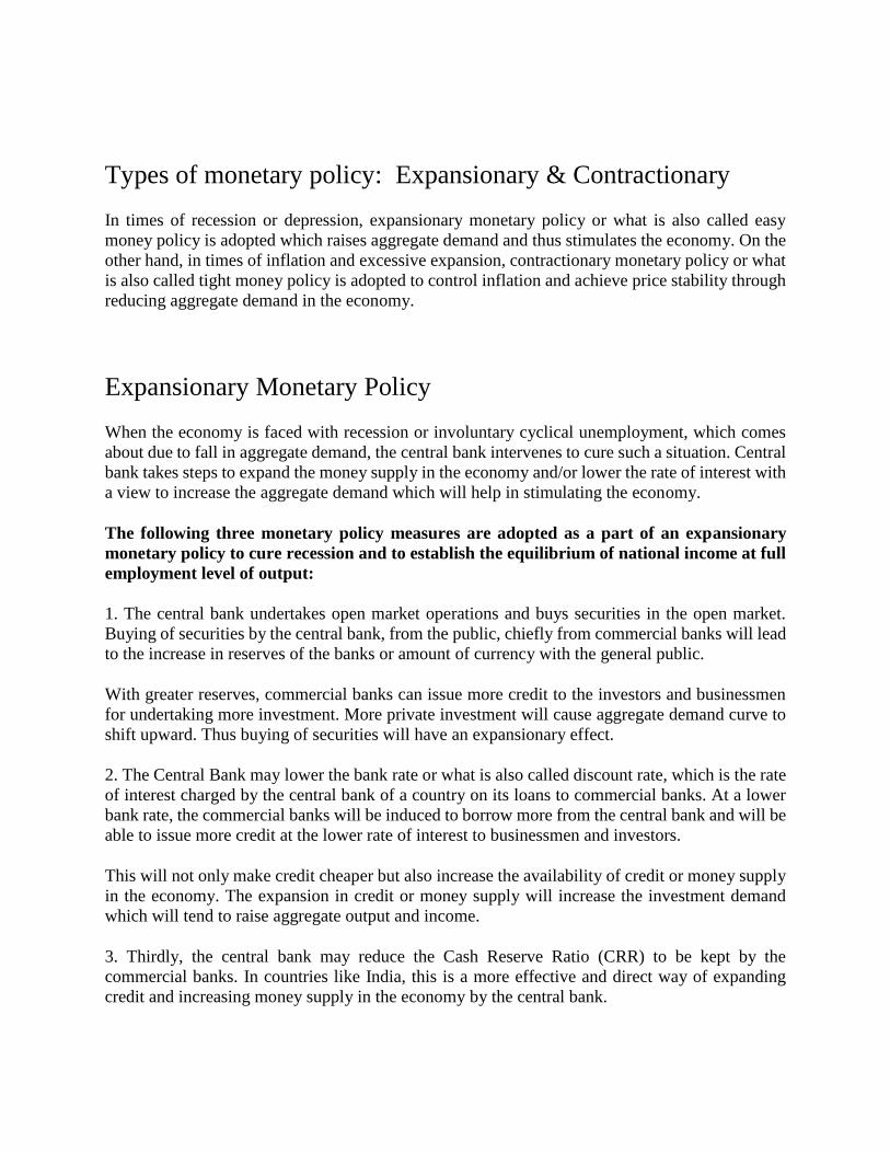
Types of monetary policy: Expansionary & Contractionary

In times of recession or depression, expansionary monetary policy or what is also called easy

money policy is adopted which raises aggregate demand and thus stimulates the economy. On the

other hand, in times of inflation and excessive expansion, contractionary monetary policy or what

is also called tight money policy is adopted to control inflation and achieve price stability through

reducing aggregate demand in the economy.

Expansionary Monetary Policy

When the economy is faced with recession or involuntary cyclical unemployment, which comes

about due to fall in aggregate demand, the central bank intervenes to cure such a situation. Central

bank takes steps to expand the money supply in the economy and/or lower the rate of interest with

a view to increase the aggregate demand which will help in stimulating the economy.

The following three monetary policy measures are adopted as a part of an expansionary

monetary policy to cure recession and to establish the equilibrium of national income at full

employment level of output:

1. The central bank undertakes open market operations and buys securities in the open market.

Buying of securities by the central bank, from the public, chiefly from commercial banks will lead

to the increase in reserves of the banks or amount of currency with the general public.

With greater reserves, commercial banks can issue more credit to the investors and businessmen

for undertaking more investment. More private investment will cause aggregate demand curve to

shift upward. Thus buying of securities will have an expansionary effect.

2. The Central Bank may lower the bank rate or what is also called discount rate, which is the rate

of interest charged by the central bank of a country on its loans to commercial banks. At a lower

bank rate, the commercial banks will be induced to borrow more from the central bank and will be

able to issue more credit at the lower rate of interest to businessmen and investors.

This will not only make credit cheaper but also increase the availability of credit or money supply

in the economy. The expansion in credit or money supply will increase the investment demand

which will tend to raise aggregate output and income.

3. Thirdly, the central bank may reduce the Cash Reserve Ratio (CRR) to be kept by the

commercial banks. In countries like India, this is a more effective and direct way of expanding

credit and increasing money supply in the economy by the central bank.

With lower reserve requirements, a large amount of funds is released for providing loans to

businessmen and investors. As a result, credit expands and investment increases in the economy

which has an expansionary effect on output and employment.

Similar to the Cash Reserve Ratio (CRR), in India there is another monetary instrument, namely,

Statutory Liquidity Ratio (SLR) used by the Reserve Bank to change the lending capacity and

therefore credit availability in the economy.

According to Statutory Liquidity Ratio, in addition to the Cash Reserve Ratio (CRR) banks have

to keep a certain minimum proportion of their deposits in the form of some specified liquid assets

such as Government securities.

To increase the lendable resources of the banks, Reserve Bank can lower this Statutory Liquidity

Ratio (SLR). Thus, when Reserve Bank of India lowers statutory liquidity Ratio (SLR), the, credit

availability for the private sector will increase.

It may be noted that the use of all the above tools of monetary policy leads to an increase in reserves

or liquid resources with the banks. Since reserves are the basis on which banks expand their credit

by lending, the increase in reserves raises the money supply in the economy. Thus, appropriate

monetary policy at times of recession or depression can increase the availability of credit and also

lower the cost of credit. This leads to more private investment spending which has an expansionary

effect on the economy.

How Expansionary Monetary Policy Works

Now, it is important to understand how expansionary monetary policy works to cause increase in

output and employment and thus help the economy to recover from recession. Rate of interest is

determined by the demand for and supply of money.

Expansion in money supply causes the rate of interest to fall. And this fall in the rate of interest

will encourage businessmen to borrow more for investment spending. As is well known, rate of

interest is the opportunity cost of funds invested for purchasing capital goods.

As rate of interest falls, it becomes profitable to invest more in producing or buying capital goods.

Thus, fall in the rate of interest raises the investment expenditure which is an important component

of aggregate demand. The increase in aggregate demand causes expansion in aggregate output,

national income and employment.

How expansion in money supply can help to cure recession is illustrated in Fig. 29.1. In panel (a)

of Fig. 29.1 it will be seen that when as a result of some measures taken by the central bank, the

money supply increases from M1 to M2, the rate of interest falls from r1 to r2.

It will be seen from panel (b) that with this fall in rate of interest, investment increases from I1 to

I2. Now, in panel (c), it is shown how the increase in investment expenditure from I1, to I2 shifts

the aggregate demand curve (C + I1 + G) upward so that the new aggregate demand curve C + I2

+ G intersects the 45° line at point E2 and thus establishes equilibrium at full-employment output

level YF.

It may be noted that with the given increase in investment how much aggregate output or

national income will increase depends on the size of income multiplier which is determined

by marginal propensity to consume. The greater the size of multiplier, the greater the impact of

increment in investment on expansion of output and income.

From above, it is clear that monetary policy can play an important role in stimulating the economy

and ensuring stability at full employment level.

Contractionary Monetary Policy

When aggregate demand rises sharply due to large consumption and investment expenditure or,

more importantly, due to the large increase in Government expenditure relative to its revenue

resulting in huge budget deficits, a demand-pull inflation occurs in the economy.

Besides, when there is too much creation of money for one reason or the other, it generates infla-

tionary pressures in the economy. To check the demand-pull inflation which has been a major

problem in India and several other countries in recent years the adoption of contractionary

monetary policy which is popularly called tight monetary policy is called for. Note that tight or

restrictive money policy is one which reduces the availability of credit and also raises its cost.

The following monetary measures which constitute tight money policy are generally adopted

to control inflation:

1. The Central Bank sells the Government securities to the banks, other depository institutions and

the general public through open market operations. This action will reduce the reserves with the

banks and liquid funds with the general public. With less reserve with the banks, their lending

capacity will be reduced. Therefore, they will have to reduce their demand deposits by refraining

from giving new loans as old loans are paid back. As a result, money supply in the economy will

shrink.

2. The bank rate may also be raised which will discourage the banks to take loans from the central

bank. This will tend to reduce their liquidity and also induce them to raise their own lending rates.

Thus this will reduce the availability of credit and also raise its cost. This will lead to the reduction

in investment spending and help in reducing inflationary pressures.

3. The most important anti-inflationary measure is the raising of statutory Cash Reserve Ratio

(CRR). To meet the new higher reserve requirements, banks will reduce their lendings. This will

have a direct effect on the contraction of money supply in the economy and help in controlling

demand-pull inflation. Besides Cash Reserve Ratio (CRR), the Statutory Liquidity Ratio (SLR)

can also be increased through which excess reserves of the banks are mopped up resulting in

contraction in credit.

4. Fourthly, an important anti-inflationary measure is the use of qualitative credit control, namely,

raising of minimum margins for obtaining loans from banks against the stocks of sensitive

commodities such as food-grains, oilseeds, cotton, sugar, vegetable oil. As a result of this measure,

businessmen themselves will have to finance to a greater extent the holding of inventories of goods

and will be able to get less credit from banks. This selective credit control has been extensively

used in India to control inflationary pressures.

How the contractionary Monetary Policy Works

It is important to understand how tight monetary policy works to check inflation. As explained

above, tight monetary policy seeks to reduce the money supply through contraction of credit in the

economy and also raising the cost of credit, that is, lending rates of interest. The reduction in

money supply itself raises the rate of interest.

The higher interest rate reduces investment spending which results in lowering of aggregate

demand curve (C + I + G). The decrease in aggregate demand tends to restrain demand-pull

inflation. How tight money policy helps in checking inflation is graphically shown in Fig. 29.2.

Let us assume that full-employment level of national income is YF as depicted in panel (c) of fig.

29.2. Now,

if due to a large budget deficit and excessive creation of money supply, aggregate demand curve

shifts to C + I2 + G2; inflationary gap of E1H comes to exist at full-employment level. That is, the

sum of consumption expenditure, private investment spending and Government expenditure

exceeds the full-employment level of output by E1H.

This creates a demand-pull inflation causing rise in prices. Though with aggregate demand curve

C + I2 + G2 equilibrium reaches at point E2 and as a result national income increases but only in

money terms; real income or output level remaining constant at OYF.

Now, it will be seen from panel (a) that if tight money policy succeeds in reducing money supply

from M2 to M1 the rate of interest will rise from r1 to r2. Panel (b) of Fig. 29.2 shows that at a

higher interest rate r2, private investment falls from I2 to This reduction in investment expenditure

shifts aggregate demand curve C + I2 + G2 downward to C + I1+ G2 and in this way inflationary

gap is closed and equilibrium at full-employment output level YF is once again established.

In our figure it has been assumed that contraction of money supply from M2 to M1 and as a result

rise in rate of interest from r1 to r2 is sufficient to reduce investment expenditure equal to I2 – I1

which is equal to inflationary gap and in this way macroeconomic equilibrium without any

inflationary pressure is established at output level YF.

It should be further remembered that in our analysis of the successful working of the tight monetary

policy it is assumed that demand for money curve (i.e., liquidity preference curve) is fairly steep

so as to push up the rate of interest from r1 to r2 and further that investment demand curve II in

panel (b) of Fig. 29.2 is fairly elastic so that rise in rate of interest from r1 to r2 is sufficient to

reduce investment by I2 – I1 or ∆I.

If these conditions regarding the shapes of the money demand curve and investment demand curve

represent the real world situation, then tight monetary policy will succeed in controlling inflation

and ensuring price stability.