notes 7 – modern lubrication theory - tribgroup …rotorlab.tamu.edu/me626/notes_pdf/notes07...
TRANSCRIPT

1
Luis San AndresMast-Childs ProfessorSept 2009
Notes 7 – Modern Lubrication Theory
Thermal analysis of finite length journal bearings including fluid inertia

Notes 7. THERMAL ANALYSIS OF FINITE LENGTH JOURNAL BEARINGS. Dr. Luis San Andrés © 2009 1
NOTES 7 THERMAL ANALYSIS OF FINITE LENGTH JOURNAL BEARINGS
INCLUDING FLUID INERTIA EFFECTS Notes 4 and 5 presented the derivation of the pressure field, load capacity and dynamic force
coefficients in a short length cylindrical journal bearing. Notes 7 present an analysis for the
prediction, using numerical methods, of the static load capacity and dynamic force coefficients in
finite-length journal bearings. Practical bearing geometries include lubricant feeding
arrangements (grooves and holes), multiple pads with mechanical preloads to enhance their load
capacity and stability. The analysis includes the evaluation of the film mean temperature field
from an energy transport equation. The film temperature affects the viscosity of the lubricant
within the fluid flow region. In addition, the analysis includes temporal fluid inertia effects
modifying the classical Reynolds equation; and hence, the model predicts not only stiffness and
damping force coefficients but also added mass coefficients. As recent test data shows, fluid
inertia effects cannot longer be ignored in journal bearing forced performance, static or dynamic.
Introduction
Analysis of the dynamic performance of rotors supported on fluid film bearings relies not just
on the rotor structural (mass and elastic) properties but also on the acurate evaluation of the static
and dynamic forced performance characteristics of the bearing supports. A rotordynamic analysis
delivers synchronous response to imbalance and stability results in accordance with API
requirements, to demonstrate certain performance characteristics ; and on occasion, to reproduce
peculiar field phenomena and to troubleshoot malfunctions or limitations of the operating
system.
Mineral-oil lubricated bearings support most commercial machinery that operate at low to
moderately high rotational shaft speeds. The bearings carry heavy static loads, mainly a fraction
of the rotor weight. The lubricant, supplied from an external reservoir, fills the small clearance
separating the shaft (journal) from the bearing. Shaft rotation drags the lubricant through the
bearing film lands to form the hydrodynamic wedge that generates the hydrodynamic fluid film
pressure that, acting on the journal, is able to support or carry the applied static load. The mineral
oil lubricant, generally of large viscosity, increases its temperature as it carries away the

Notes 7. THERMAL ANALYSIS OF FINITE LENGTH JOURNAL BEARINGS. Dr. Luis San Andrés © 2009 2
mechanical energy dissipated into heat. Hence, the material visosity of the lubricant, a strong
function of temperature, does not remain constant within the film flow region in the bearing.
Importantly enough, the conditions of low speed (Ω), small clarance (c), and large viscosity
(μ/ρ) determine a laminar flow condition in the bearing, i.e. operation with small Reynolds
numbers Re < 1,000 (Re=ρΩRc/μ). Hence, Reynolds equation of Classical Lubrication is valid
for prediction of the equilibrium hydrodynamic film pressure in the bearing. The prediction of
the thermal energy transport in a thin film bearing is more difficult since there is a significant
temperature along and accross the film, i.e. a three-dimensional phenomenon. Most importantly,
the thermal energy exchange does not just involve the mechanical energy generated by shear and
its advection by the lubricant flow but also must account for the heat conduction into or from the
shaft and bearing cartridge.
A comprehensive 3-D thermohydrodynamic analysis for prediction of performance in finite
length journal bearings is out of the scope of these lecture notes. The interested reader should
refer to relevant work in the archival literature [1,2] for further details. However, note that most
fluid film bearing designers and bearing manufacturers rarely rely on cumbersome and
computationally expensive analysis tools; in particular when these require of boundary
conditions that are operating system dependent (not general). More than often, engineers prefer
to obtain model results that are in agreement with published test data and go along with their vast
practical experience.
Notes 7. THERMAL ANALYSIS OF FINITE LENGTH JOURNAL BEARINGS. Dr. Luis San Andrés © 2009 3
Analysis
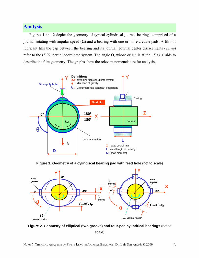
Figures 1 and 2 depict the geometry of typical cylindrical journal bearings comprised of a
journal rotating with angular speed (Ω) and a bearing with one or more arcuate pads. A film of
lubricant fills the gap between the bearing and its journal. Journal center dislacements (eX, eY)
refer to the (X,Y) inertial coordinate system. The angle Θ, whose origin is at the –X axis, aids to
describe the film geometry. The graphs show the relevant nomenclature for analysis.
X
gjournal rotation
0º -180º180º
Definitions:X,Y: fixed (inertial) coordinate systemg : direction of gravity
Circumferential (angular) coordinateOil supply hole
Z : axial coordinate L : axial length of bearingD: shaft diameter
D
Y
Z
L
Journal
Casing
Y
Fluid film
Figure 1. Geometry of a cylindrical bearing pad with feed hole (not to scale)
journal rotation
X
Axial groove
0º
-90º
-180º
Y
rP, preload
Cmin=C-rP
0º
Journal rotation
X
-180º
Y
rP, preload
Cmin=C-rP
Axial groove
journal rotation
X
Axial groove
0º
-90º
-180º
Y
rP, preload
Cmin=C-rP
0º
Journal rotation
X
-180º
Y
rP, preload
Cmin=C-rP
Axial groove
Figure 2. Geometry of elliptical (two groove) and four-pad cylindrical bearings (not to
scale)

Notes 7. THERMAL ANALYSIS OF FINITE LENGTH JOURNAL BEARINGS. Dr. Luis San Andrés © 2009 4
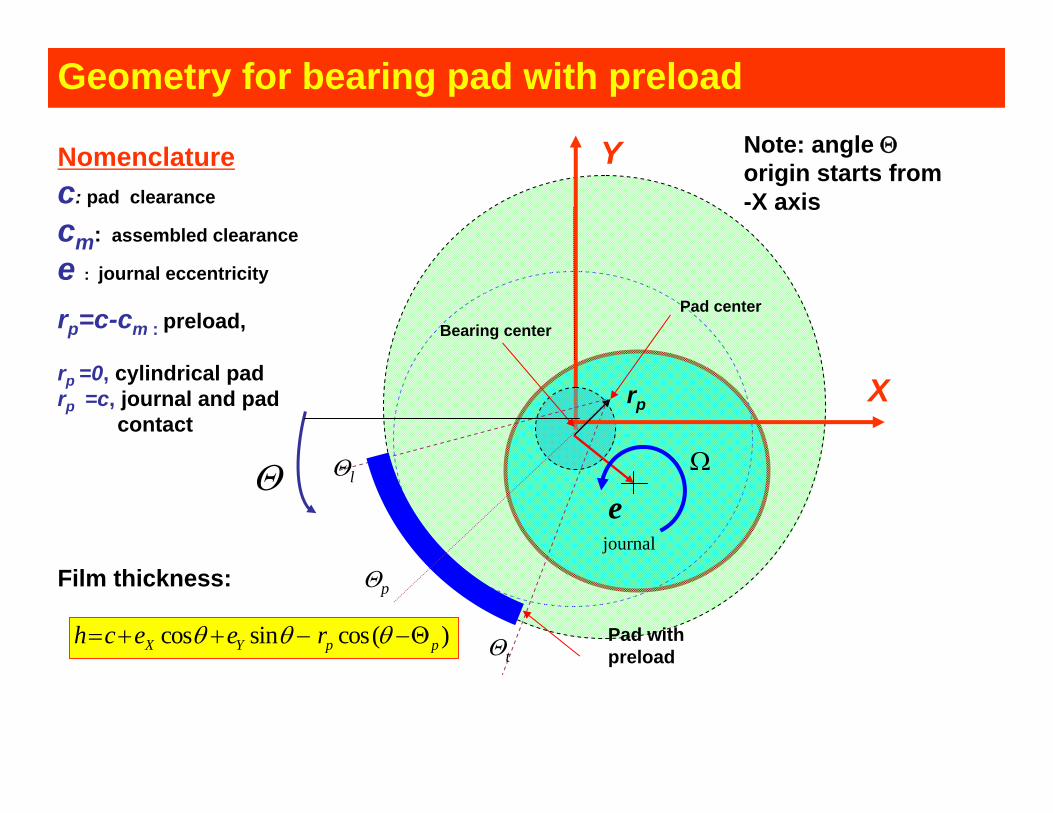
Figure 3 shows a typical bearing pad with radial clearance (c) and preload (rp) at angle ΘP. Θl
and Θt denote the leading edge and trailing edges of the pad, respectively. Within the flow region
, 0l t z L , the film thickness (h) is
cos( ) cos sinp p X Yt th c r e e (1)
where ,X Y te e are the journal center eccentricity components along the (X, Y) directions.
rp=c-cm : preload,
rp =0, cylindrical pad rp =c, journal and pad
contact
Nomenclaturec: pad clearance
cm: assembled clearance
e : journal eccentricity
Film thickness:
l
p
t
X
Y
journal
e
Pad centerBearing center
Pad with preload
rp
cos sin cos( )X Y p ph c e e r
rp=c-cm : preload,
rp =0, cylindrical pad rp =c, journal and pad
contact
Nomenclaturec: pad clearance
cm: assembled clearance
e : journal eccentricity
Film thickness:
l
p
t
X
Y
journal
e
Pad centerBearing center
Pad with preload
rp
cos sin cos( )X Y p ph c e e r
Figure 3. Geometry of a bearing pad with preload and description of film thickness (not to scale)
Governing equations for pressure generation and temperature transport The modified [3,4,5] laminar flow Reynolds equation describing the generation of
hydrodynamic pressure (P) in the thin film region , 0l t z L of a bearing pad is
3 3 2 2
2 2( ) ( ) ( )
1
12 12 2 12T T T
h P h P h h h h
R z z t t
(2)
rp=c-cm : preload,
rp =0, cylindrical pad rp =c, journal and pad
contact
Nomenclaturec: pad clearance
cm: assembled clearance
e : journal eccentricity
Film thickness:
Geometry for bearing pad with preload
l
p
t
X
Y
journal
e
Pad centerBearing center
Pad with preload
rp
cos sin cos( )X Y p ph c e e r
Note: angle origin starts from -X axis

Ask about:
What is a pad preload?
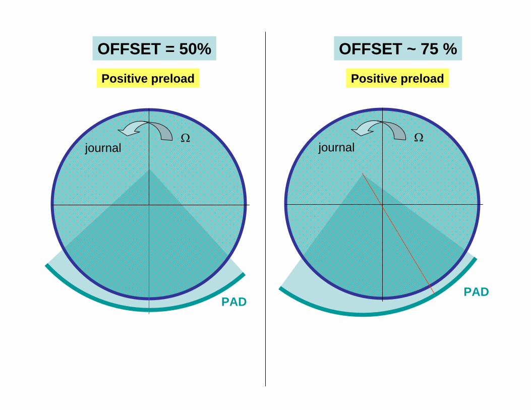
What is the pad offset?

journal
PAD

Positive preload
journal
Zero preload
journal
PAD
PAD
OFFSET = 50%

Positive preload
journal
negative preload
journal
PAD
PAD
OFFSET = 50%
Positive preload
journal
Positive preload
journal
PADPAD
OFFSET = 50% OFFSET ~ 75 %

Positive preload
journal
Positive preload
journal
PAD
PAD
OFFSET = 50% OFFSET ~ 25 %

Notes 7. THERMAL ANALYSIS OF FINITE LENGTH JOURNAL BEARINGS. Dr. Luis San Andrés © 2009 5
where (ρ, μ) denote the lubricant density and viscosity, both temperature (T) dependent material
properties. For example, v ST TS e , with subindex S denoting supply conditions. The
modified Reynolds equation includes temporal fluid inertia effects ; hence, the flow model is
strictly applicable to lubricant thin film flows induced by small amplitude journal motions about
an equilibrium position.
For the laminar flow of an incompressible fluid and regarding the temperature as uniform
along the axial direction, the energy transport equation under steady-state conditions is [6]
22 2
212
12 2v s
R RC hU T hW T Q S W U
R z h
(3)
where T is the lubricant bulk-temperature1 and s B B J JQ h T T h T T is the heat flow
into the bearing and journal surfaces. Above, Cv is the lubricant specific heat, and (W, U)
represent the axial and circumferential mean flow velocities given by
2 2
;12 12 2
h P h P RW U
z R
(4)
Eq. (3) is representative of a bulk-flow model that balances the mechanical shear dissipation
energy (S) to the thermal energy transport due to advection by the fluid flow and convection (Qs)
into the bearing surfaces. The heat convection coefficients ,B Jh h depend on the Prandtl
number (r vP C
) and the flow condition defined by the local Reynolds number e
U hR
relative to the bearing and journal surfaces[7]. For laminar flow, 1e
cR
R , Colburn’s analogy
renders the convection coefficients 1
33 rh Ph
. See Ref. [8] for details2.
1 The bulk temperature represents an average across the film thickness, i.e. , ,0
1 h
z yT T dyh
2 The THD model implements a number of heat transfer models, including those for fixed or developing wall temperatures and heat flows.
Notes 7. THERMAL ANALYSIS OF FINITE LENGTH JOURNAL BEARINGS. Dr. Luis San Andrés © 2009 6
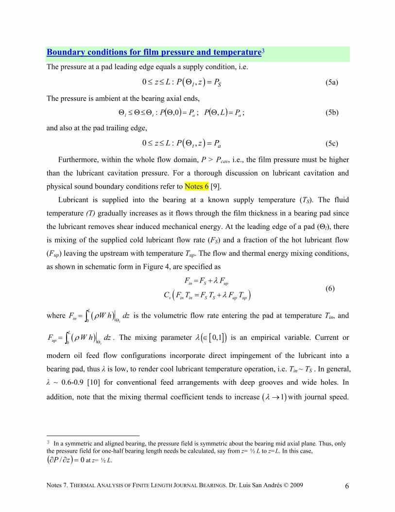
Boundary conditions for film pressure and temperature3
The pressure at a pad leading edge equals a supply condition, i.e.
0 : , l Sz L P z P (5a)
The pressure is ambient at the bearing axial ends,
;, ; 0,: aatl PLPPP (5b)
and also at the pad trailing edge,
0 : , t az L P z P (5c)
Furthermore, within the whole flow domain, P > Pcav, i.e., the film pressure must be higher
than the lubricant cavitation pressure. For a thorough discussion on lubricant cavitation and
physical sound boundary conditions refer to Notes 6 [9].
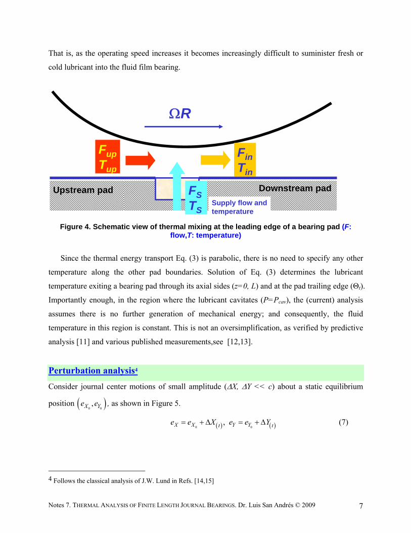
Lubricant is supplied into the bearing at a known supply temperature (TS). The fluid
temperature (T) gradually increases as it flows through the film thickness in a bearing pad since
the lubricant removes shear induced mechanical energy. At the leading edge of a pad (Θl), there
is mixing of the supplied cold lubricant flow rate (FS) and a fraction of the hot lubricant flow
(Fup) leaving the upstream with temperature Tup. The flow and thermal energy mixing conditions,
as shown in schematic form in Figure 4, are specified as
in S up
v in in S S up up
F F F
C F T F T F T
(6)
where 0 l
L
inF W h dz
is the volumetric flow rate entering the pad at temperature Tin, and
0 t
L
upF W h dz
. The mixing parameter 0,1 is an empirical variable. Current or
modern oil feed flow configurations incorporate direct impingement of the lubricant into a
bearing pad, thus λ is low, to render cool lubricant temperature operation, i.e. Tin ~ TS . In general,
λ ~ 0.6-0.9 [10] for conventional feed arrangements with deep grooves and wide holes. In
addition, note that the mixing thermal coefficient tends to increase 1 with journal speed.
3 In a symmetric and aligned bearing, the pressure field is symmetric about the bearing mid axial plane. Thus, only the pressure field for one-half bearing length needs be calculated, say from z= ½ L to z=L. In this case,
0/ zP at z= ½ L.
Notes 7. THERMAL ANALYSIS OF FINITE LENGTH JOURNAL BEARINGS. Dr. Luis San Andrés © 2009 7
That is, as the operating speed increases it becomes increasingly difficult to suminister fresh or
cold lubricant into the fluid film bearing.
Upstream pad Downstream pad
R
FupTup
FinTin
FSTS
Supply flow and temperature
Figure 4. Schematic view of thermal mixing at the leading edge of a bearing pad (F: flow,T: temperature)
Since the thermal energy transport Eq. (3) is parabolic, there is no need to specify any other
temperature along the other pad boundaries. Solution of Eq. (3) determines the lubricant
temperature exiting a bearing pad through its axial sides (z=0, L) and at the pad trailing edge (Θt).
Importantly enough, in the region where the lubricant cavitates (P=Pcav), the (current) analysis
assumes there is no further generation of mechanical energy; and consequently, the fluid
temperature in this region is constant. This is not an oversimplification, as verified by predictive
analysis [11] and various published measurements,see [12,13].
Perturbation analysis4
Consider journal center motions of small amplitude (X, Y << c) about a static equilibrium
position 0 0,X Ye e , as shown in Figure 5.
0 0,X X Y Yt te e X e e Y (7)
4 Follows the classical analysis of J.W. Lund in Refs. [14,15]

Notes 7. THERMAL ANALYSIS OF FINITE LENGTH JOURNAL BEARINGS. Dr. Luis San Andrés © 2009 8
Wo X
Y
eXo
eY
eo
X
clearancecircle
YStatic load
Journal center
Wo X
Y
eXo
eY
eo
X
clearancecircle
YStatic load
Journal center
Figure 5. Depiction of small amplitude journal motions about an equilibrium position (Not to scale).
The film thickness is expressed as the superposition of an equilibrium (zeroth-order)
thickness (h0) and a first-order thickness (h1), i.e.
0 1 th h h ,
0 00 cos( ) cos sinp p X Yh c r e e , (8)
sincos1 tt YXh ,
with
0 0
0 1( ) ( )sin( ) sin cos ; sin cosp p X Y t t
h hr e e X Y
2
2cos sin , cos sin
h hX Y X Y
t t
(9)
The perturbation in film thickness leads naturally to a perturbation in film pressure, i.e.

Notes 7. THERMAL ANALYSIS OF FINITE LENGTH JOURNAL BEARINGS. Dr. Luis San Andrés © 2009 9
0 1
1
( , , ) ( , ) ( , , ),
X Y X Y X Y
P z t P z P z t
P P X P Y P X P Y P X P Y
(10)
where P0 is the zeroth-order or equilibrium pressure field defined by 0 0,X Ye e at steady
operating conditions, and ΔP1 is the perturbed dynamic pressure field5.
Define the linear operator
3 30 0
() ()1()
12 12
h h
R R z z
L (11)
Substitution of the pressure (P) and film thickness (h) into the modified Reynolds Eq. (2)
gives the following equations for determination of the equilibrium and first order pressure fields
3 30 0 0 0 0
0 2
1( )
12 12 2
h P h P hRP
R z z R
L (12a)
2 20 0 0 0
2 20 0 0 0
3 3cos cos
2 12 12
3 3sin sin
2 12 12
X
Y
h P h PRP
R R z z
h P h PRP
R R z z
L
L
(12b)
cos ; sinX YP P L L (12c)
2 20 0cos ; sin
12 12X Y
h hP P
L L (12d)
where 0 00 cos( ) cos sinp p X Yh c r e e .
The boundary conditions for the solution of the zeroth- and first-order pressure fields
follow. Note that in those boundaries where the pressure is fixed, say at ambient condition, the
perturbed pressures must vanish, i.e. a homogeneous boundary condition. Hence,
P0(l ,0<z<L) = PS ; P0 (t , 0<z<L) = Pa
0 0: ,0 ; , ;l t a aP P P L P (13a)
, , , , ,0 , , ,0
l tX Y X Y X Y z z L
P P P P P P
(13b)
5 The physical units of each perturbed pressure differ. For example,
2, , , , ,X Y X Y X YPa Pa PaP P P P P Pm m s m s

Notes 7. THERMAL ANALYSIS OF FINITE LENGTH JOURNAL BEARINGS. Dr. Luis San Andrés © 2009 10
At the inception of the film rupture or cavitation zone (c), P0=Pcav, and 0 0P . At
this location, the first-order pressure fields also vanish, i.e. 0.X Y X Y X YP P P P P P
Other physical conditions may also apply6.
The current analysis does not consider a perturbation in the temperature field or the lubricant
material properties (density and viscosity). Recall the journal motions are small in amplitude
affecting little the steady-state temperature field. However, in bearings and seals operating in the
turbulent flow regime, the journal motion does affect the flow condition and hence, there is the
need to account for temporal variations in the fluid material viscosity and density, see Notes 10
[6]
Bearing reaction forces and force coefficients
The hydrodynamic pressure field generated in each pad acts on the journal to generate a fluid
film reaction force with components ,X YF F . Integration of the pressure fields gives
( , , )1 1 0
cos
sin
tpads padk
k
k l
N N LXX
z t kY Yk k k
FFP R d dz
F F
(14)
Substitution of Eq. (10) gives for the kth pad
1
0
0
cos
sin
tL
XX Y X Y X Y k
Y k
FP P X P Y P X P Y P X P Y R d dz
F
(15)
The components of a pad reaction force are expressed in terms of stiffness, damping and
inertia force coefficients (K, C, M)αβ=X,Y
0
0
( )
( )
XX t XX XY XX XY XX XY
YX YY YX YY YX YYY t Y k k kk k
FF K K C C M MX X X
K K C C M MF F Y Y Y
(16)
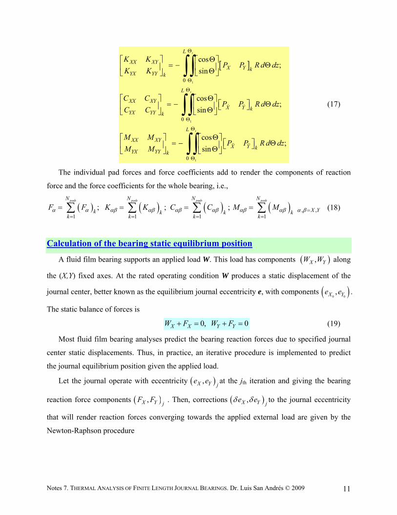
The bearing pad force coefficients follow from
6 See for example, Zhang, Y., 1990, “Starting Pressure Boundary Conditions for Perturbed Reynolds Equation,” ASME Journal of Lubrication Technology, Vol. 112, pp. 551-556.
Notes 7. THERMAL ANALYSIS OF FINITE LENGTH JOURNAL BEARINGS. Dr. Luis San Andrés © 2009 11
1
1
1
0
0
0
cos;
sin
cos;
sin
cos;
sin
t
t
t
L
XX XYX Y k
YX YY k
L
XX XYX Y k
YX YY k
L
XX XYX Y k
YX YY k
K KP P R d dz
K K
C CP P R d dz
C C
M MP P R d dz
M M
(17)
The individual pad forces and force coefficients add to render the components of reaction
force and the force coefficients for the whole bearing, i.e.,
, ,1 1 1 1
; ; ;pads pads pads padsN N N N
X Yk k k kk k k k
F F K K C C M M
(18)
Calculation of the bearing static equilibrium position
A fluid film bearing supports an applied load W. This load has components ,X YW W along
the (X,Y) fixed axes. At the rated operating condition W produces a static displacement of the
journal center, better known as the equilibrium journal eccentricity e, with components 0 0,X Ye e .
The static balance of forces is
0, 0X X Y YW F W F (19)
Most fluid film bearing analyses predict the bearing reaction forces due to specified journal
center static displacements. Thus, in practice, an iterative procedure is implemented to predict
the journal equilibrium position given the applied load.
Let the journal operate with eccentricity ,X Y je e at the jth iteration and giving the bearing
reaction force components ,X Y jF F . Then, corrections ,X Y j
e e to the journal eccentricity
that will render reaction forces converging towards the applied external load are given by the
Newton-Raphson procedure

Notes 7. THERMAL ANALYSIS OF FINITE LENGTH JOURNAL BEARINGS. Dr. Luis San Andrés © 2009 12
j
jj
YY
XX
jYYYX
XYXX
jY
X
FW
FW
KK
KK
e
e 1
(20a)
and
jY
X
jY
X
jY
X
e
e
e
e
e
ejjj
1
1 (20b)
Aboce, the bearing pseudo or temporal stiffness coefficients (Kαβ=X,Y) are evaluated at ,X Y je e .
Upon convergence, the differences in forces in Eq. (19) become negligible, i.e. (W+F)X,Y 0;
and the stiffness coefficients are those of the bearing at its equilibrium position.
Note that the bearing reaction forces are highly nonlinear functions of the journal position or
eccentricity function; thus, convergence of the Newton-Raphson algorithm relies heavily on the
closeness of the initial journal eccentricity components to the actual equilibrium eccentricity. Of
course, the fact noted is common in the solution of any nonlienar system of equations.
Generalization of the perturbation method
Consider small amplitude harmonic journal motions ,X Ye e with whirl frequency
about the equilibrium position 0 0,X Ye e . The film thickness (h) is the real part of the following
expression
0 0 ,cos sin ; ; 1t tX Y X Yh h e e e h e h e
i i i (21)
with h0 as the equilibrium film thickness at 0 0,X Ye e , and cos , sinX Yh h . Note that,
2
0 22
,
tt t
h e h eh he h e e h e
t t t
ii ii (22)
The pressure field is written as the superposition of zeroth and first order fields,
0 , ; tX YP P e P e
i. (23)
The zeroth-order (P0) is the equilibrium pressure field satisfying
3 30 0 0 0 0
0 2
1( )
12 12 2
h P h P hRP
R z z R
L (24=12a)
Notes 7. THERMAL ANALYSIS OF FINITE LENGTH JOURNAL BEARINGS. Dr. Luis San Andrés © 2009 13
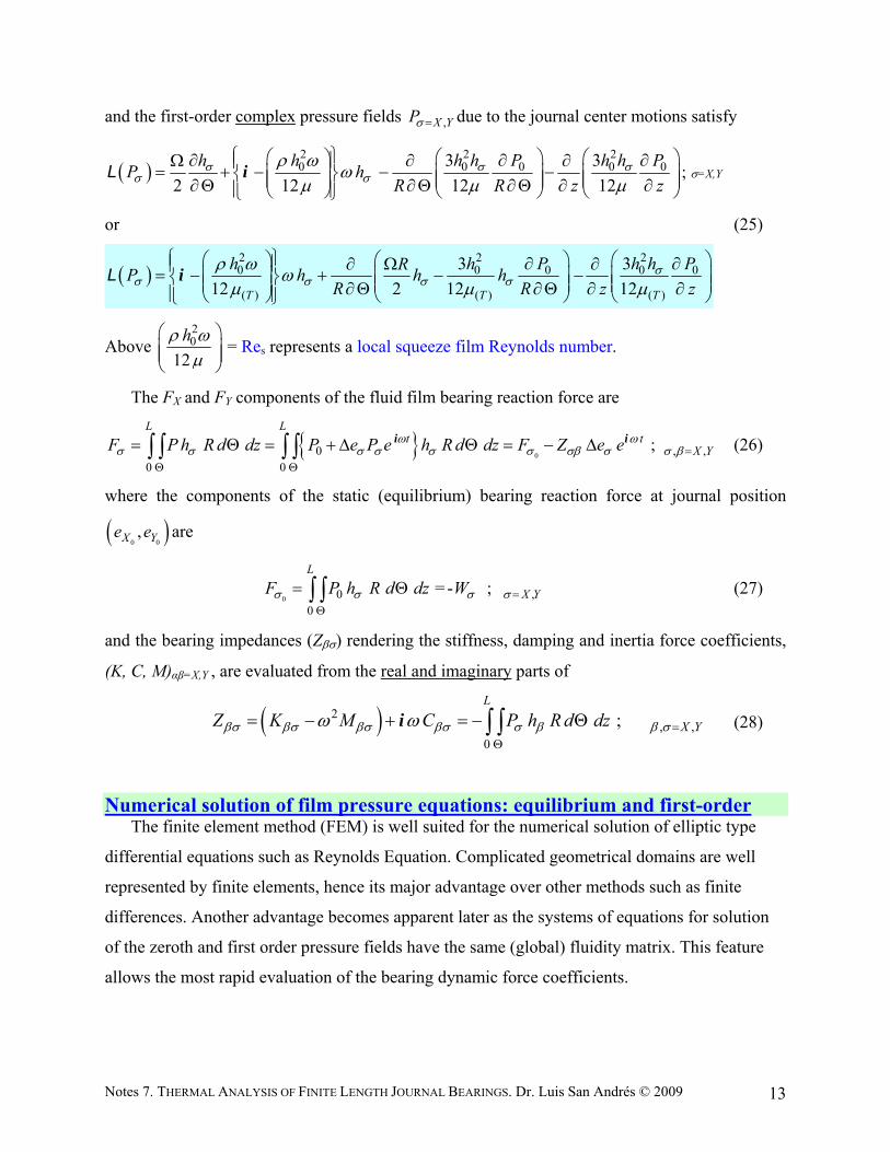
and the first-order complex pressure fields ,X YP due to the journal center motions satisfy
2 2 20 0 0 0 03 3
2 12 12 12
h h h h P h h PP h
R R z z
L i ; =X,Y
or (25)
2 2 20 0 0 0 0
( ) ( ) ( )
3 3
12 2 12 12T T T
h h P h h PRP h h h
R R z z
L i
Above 20
12
h
= Res represents a local squeeze film Reynolds number.
The FX and FY components of the fluid film bearing reaction force are
00 , ,
0 0
; L L
t tX YF P h R d dz P e P e h R d dz F Z e e
i i (26)
where the components of the static (equilibrium) bearing reaction force at journal position
0 0,X Ye e are
0 0 ,0
= - ; L
X YF P h R d dz W
(27)
and the bearing impedances (Z) rendering the stiffness, damping and inertia force coefficients,
(K, C, M)αβ=X,Y , are evaluated from the real and imaginary parts of
2, ,
0
; L
X YZ K M C P h R d dz
i (28)
Numerical solution of film pressure equations: equilibrium and first-order The finite element method (FEM) is well suited for the numerical solution of elliptic type
differential equations such as Reynolds Equation. Complicated geometrical domains are well
represented by finite elements, hence its major advantage over other methods such as finite
differences. Another advantage becomes apparent later as the systems of equations for solution
of the zeroth and first order pressure fields have the same (global) fluidity matrix. This feature
allows the most rapid evaluation of the bearing dynamic force coefficients.
Notes 7. THERMAL ANALYSIS OF FINITE LENGTH JOURNAL BEARINGS. Dr. Luis San Andrés © 2009 14
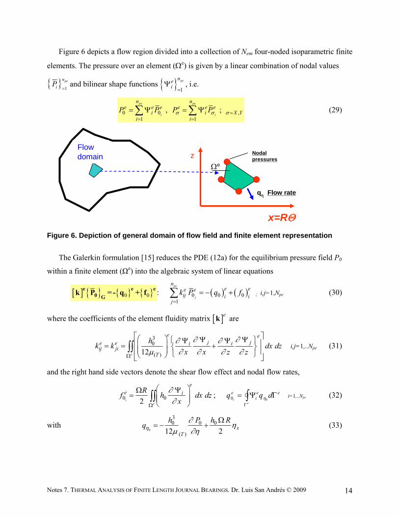
Figure 6 depicts a flow region divided into a collection of Nem four-noded isoparametric finite
elements. The pressure over an element (e) is given by a linear combination of nodal values
Pi
npe
1and bilinear shape functions
1
penei
, i.e.
0 0 ,1 1
, ; pe pe
i i
n ne e e e e e
i i X Yi i
P P P P
(29)
e
x=R
z Nodal pressures
q Flow rate
Flowdomain
Figure 6. Depiction of general domain of flow field and finite element representation
The Galerkin formulation [15] reduces the PDE (12a) for the equilibrium pressure field P0
within a finite element (Ωe) into the algebraic system of linear equations
0 0e e e
0 Gk P = - q + f : 0 0 0
1
pe
j
ne ee e
ij i ij
k P q f
; i,j=1,Npe (30)
where the coefficients of the element fluidity matrix ek are
30
( )12e
e ej je e i i
ij jiT
hk k dx dz
x x z z
i,j=1,..Npe (31)
and the right hand side vectors denote the shear flow effect and nodal flow rates,
0 0 2i
e
e
e iRf h dx dz
x
; q q d
ie
eie e
0 0
i=1,..Npe (32)
with 0
30 0 0
( )12 2 xT
h P h Rq
(33)
Notes 7. THERMAL ANALYSIS OF FINITE LENGTH JOURNAL BEARINGS. Dr. Luis San Andrés © 2009 15
as the flow through the element boundary (e). Note above that the fluid viscosity is a function
of the temperature, v ST TS e ; thys, varying over the flow domain.
The integrals in Eqns. (31, 32) are evaluated numerically over a master isoparametric
element ( ) with normalized coordinates. Reddy and Gartling [16] explain the coordinate
transformation and numerical integration procedure using Gauss-Legendre quadrature formulas.
Eqns. (30) are assembled over the whole flow domain and then condensed by enforcing the
corresponding boundary conditions. The resultant global set of equations is
0G G GGk P = Q + F (34)
where 1 1 1
, ,Nem Nem Nem
e
e e e
e e
G G Gk k Q q F f . The global fluidity matrix Gk is
symmetric, easily decomposed into its upper and lower triangular form (Cholesky algorithm), i.e.
TG G G G Gk = L U = L L (35)
A process of back- and forward-substitutions then renders the discrete zeroth order pressure
field 0 GP :
T0G G G GG
L L P = Q + F (36)
Note that G
Q 0 denotes the addition of flow rates at a node. Hence the components of
this vector are nil at each internal node of the finite element domain.
A similar procedure follows for solution of the perturbed (dynamic) pressure fields, PX and
PY, due to journal harmonic displacements ,X Ye e with whirl frequency ω. PDEs (25)
become
0 , 1 1
; pe pe
j j
n ne e ee e e
ij X Yi ij ij j
k P f S P q
i,j=1,..Npe (37)
with cos , sinX Yh h , 1 i . Defining , ,andi ii x i zx z
. Above, for
perturbations along the X-direction,
X X X X e e e e0G G
k P = f S P q (37a)
for example.

Notes 7. THERMAL ANALYSIS OF FINITE LENGTH JOURNAL BEARINGS. Dr. Luis San Andrés © 2009 16
In Equations (37)
e e e
2 20
,( )
2 12
e
e e e ei x i ii
T
hRf h dx dz h dx dz h dx dz
i
20
, , , ,( )
3
12e
eee
i x j x i z j zijT
h hS dx dz
, i,j=1,..Npe (38)
e
e e eii
q q d
; 3 20 0 0
( ) ( )
3
12 12 2 xT T
h P h h P Rq h
The assembly process of the first order FE equations renders a fluidity matrix identical to
that for the equilibrium pressure field. Thus, the perturbed pressure fields can be calculated
rapidly since the global fluidity matrix Gk is originally obtained and decomposed in the
procedure to find the equilibrium pressure field 0 GP , see Eq. (36).
In practice, the process does not require specification of a whirl frequency (ω) nor
conducting several calculations to discern the stiffnesses from the mass coefficients.
For ,X YP P from Eqs. (12b):
0 , 1 1
; pe pe
j j
n ne e ee e e
ij X Yi ij ij j
k P f S P q
i=1,..Npe (39a)
e
, 2
e ei xi
Rf h dx dz
;
20
, , , ,( )
3
12e
eee
i x j x i z j zijT
h hS dx dz
(39b)
To make the global system of equations
Tσ σ σ 0G G GG G GG
L L P = Q + F S P (39c)
For ,X YP P from Eqs. (12c):
, 1
; pe
j
ne ee e
ij X Yi ij
k P f q
i=1,..Npe (40a)
e
e e
iif h dx dz
i=1,..Npe (40b)
Giving the global system of equations
Notes 7. THERMAL ANALYSIS OF FINITE LENGTH JOURNAL BEARINGS. Dr. Luis San Andrés © 2009 17
Tσ σ GG G GG
L L P = Q + F (40c)
For ,X YP P from Eqs. (12c):
, 1
; pe
j
ne ee e
ij X Yi ij
k P f q
i=1,..Npe (41a)
e
20
( )
12
e
e eii
T
hf h dx dz
i=1,..Npe (41b)
Giving the system of equations
Tσ σ GG G GG
L L P = Q + F (41c)
Solution of the system of equations for the first order fields is performed quickly with the
procedure
find
find
T
G G G G
G G G G
T
G G G G
L L X = Y
L Z = Y Z
L X Z X
(42)
which does not require inversion of matrices but only 2-N forward and backward substitutions.
Numerical solution of the traport equation for fluid film mean temperature
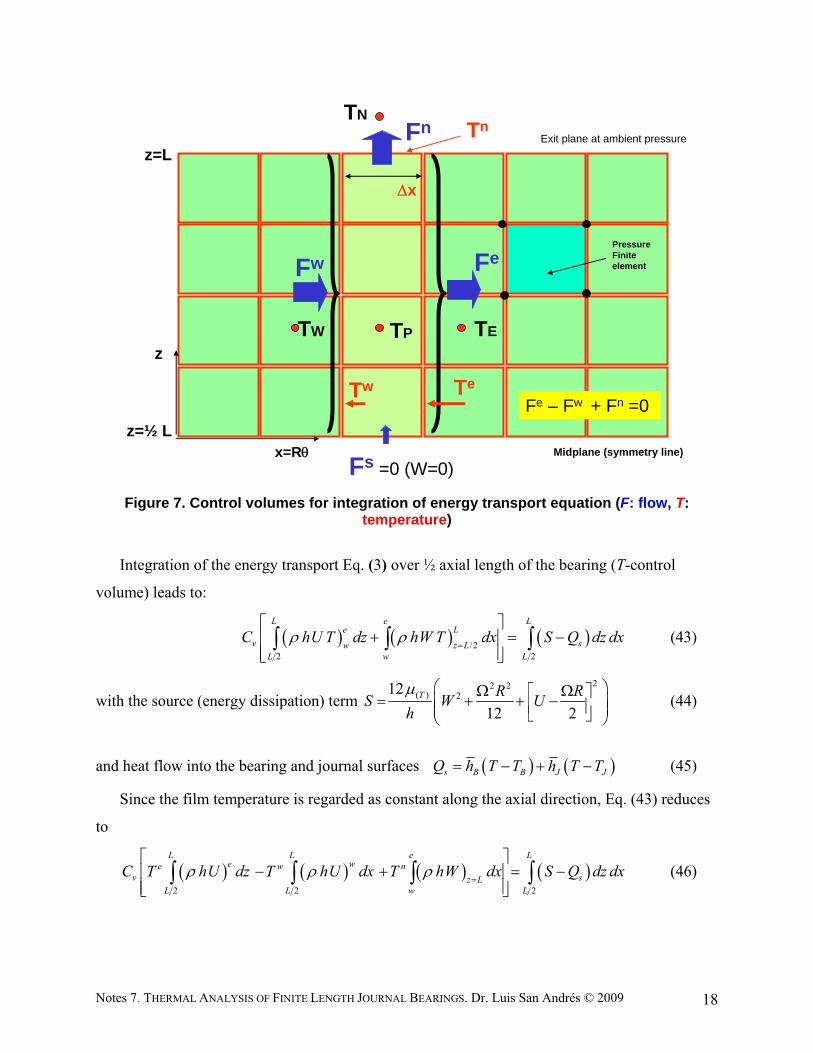
The transport of energy equation (3) is of parabolic type. Hence, a control volume method
with upwinding [17 ] is chosen to solve for the temperature field. Figure 7 depicts the control
volume for integration of the thermal energy transport Eq. (3). Note that, in accordance with
practice and measurements, the fluid bulk-temperature (T) does not vary along the bearing axial
length. In the figure, Te, Tw and Tn are temperatures at the east, west and north faces of the P-
control volume; while TE, TW, TP are nodal temperatures at the center of the control-volumes.
Notes 7. THERMAL ANALYSIS OF FINITE LENGTH JOURNAL BEARINGS. Dr. Luis San Andrés © 2009 18
z=½ L
z=L
Fs =0 (W=0) Midplane (symmetry line)
Fw Fe
Fn
Fe – Fw + Fn =0
TPTW
x
x=R
zTE
Tn
Tw Te
Exit plane at ambient pressure
PressureFinite element
TN
Figure 7. Control volumes for integration of energy transport equation (F: flow, T: temperature)
Integration of the energy transport Eq. (3) over ½ axial length of the bearing (T-control
volume) leads to:
/22 2
L e Le L
v sw z LL w L
C hU T dz hW T dx S Q dz dx
(43)
with the source (energy dissipation) term 22 2
( ) 212
12 2T R R
S W Uh
(44)
and heat flow into the bearing and journal surfaces s B B J JQ h T T h T T (45)
Since the film temperature is regarded as constant along the axial direction, Eq. (43) reduces
to
2 2 2
L L e Le we w n
v sz LL L w L
C T hU dz T hU dx T hW dx S Q dz dx
(46)
Notes 7. THERMAL ANALYSIS OF FINITE LENGTH JOURNAL BEARINGS. Dr. Luis San Andrés © 2009 19
Recall that the axial flow velocity is null7 at the midplane of a bearing pad, i.e., W=0 at z=0.
Define mass flow rates (F) through the control volume faces as
2
2
/2 0
,
,
; 0
z
z
L Nee ee
JJL
L New ww
JJL
e en s
z L zw w
F hU dz hU z
F hU dz hU z
F hW dx F hW dx
(47)
where Nez is the number of P-finite elements along the axial direction. The source term from
shear drag power is
22 2
( ) 2
2
12,
12 2
z
PL Ne
TP
JL J
R RS S dz dx W U z x
h
(48a)
From mass flow continuity 0e w nF F F =0. Assume for simplicity that the bearing
(TB) and journal (TJ) temperatures are constant along the axial direction. An identical statement is
made for the heat convection coefficients ,B Jh h . Then,
2 2 2
LP
s P B J B B J J
L
L LQ Q dz dx T h h x h T h T x (48b)
With the definitions above, the discretized algebraic form of the energy transport equation
is:
e e w w n n P P
vC F T F T F T S Q (49)
Implementation of the upwind scheme [17] for the thermal flux transport terms gives:
,0 ,0e e e eP EF T F T F T
,0 ,0w w w wW PF T F T F T (50)
,0 ,0n n nP n NF T F T F T
with 1 1,0 ; ,0 ; ,0 ,0
2 2a a a a a a a a a ;
7 This is because the pressure field is symmetric along the axial direction. That is, the peak pressure occurs at the axial mid-plane of the bearing
Notes 7. THERMAL ANALYSIS OF FINITE LENGTH JOURNAL BEARINGS. Dr. Luis San Andrés © 2009 20
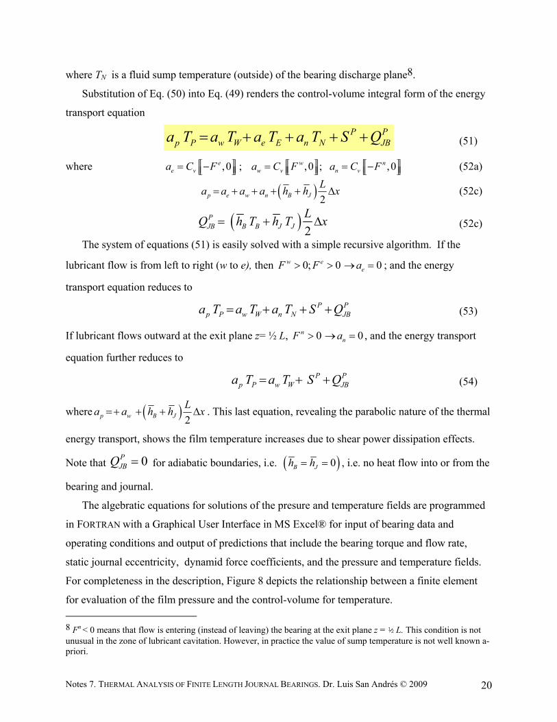
where TN is a fluid sump temperature (outside) of the bearing discharge plane8.
Substitution of Eq. (50) into Eq. (49) renders the control-volume integral form of the energy
transport equation
P P
p P w W e E n N JBa T a T a T a T S Q (51)
where ,0 ; ,0 ; ,0e w ne v w v n va C F a C F a C F (52a)
2p e w n B J
La a a a h h x (52c)
2
PJB B B J J
LQ h T h T x (52c)
The system of equations (51) is easily solved with a simple recursive algorithm. If the
lubricant flow is from left to right (w to e), then 0; 0 0w eeF F a ; and the energy
transport equation reduces to
P Pp P w W n N JBa T a T a T S Q (53)
If lubricant flows outward at the exit plane z= ½ L, 0 0nnF a , and the energy transport
equation further reduces to
P Pp P w W JBa T a T S Q (54)
where 2p w B J
La a h h x . This last equation, revealing the parabolic nature of the thermal
energy transport, shows the film temperature increases due to shear power dissipation effects.
Note that 0PJBQ for adiabatic boundaries, i.e. 0B Jh h , i.e. no heat flow into or from the
bearing and journal.
The algebratic equations for solutions of the presure and temperature fields are programmed
in FORTRAN with a Graphical User Interface in MS Excel® for input of bearing data and
operating conditions and output of predictions that include the bearing torque and flow rate,
static journal eccentricity, dynamid force coefficients, and the pressure and temperature fields.
For completeness in the description, Figure 8 depicts the relationship between a finite element
for evaluation of the film pressure and the control-volume for temperature.
8 Fn < 0 means that flow is entering (instead of leaving) the bearing at the exit plane z = ½ L. This condition is not unusual in the zone of lubricant cavitation. However, in practice the value of sump temperature is not well known a-priori.

Notes 7. THERMAL ANALYSIS OF FINITE LENGTH JOURNAL BEARINGS. Dr. Luis San Andrés © 2009 21
TPTW TE
z=L
x=R
z
West face East face
Pressure node
hU)w|e hU)w|e+1
zPressureFinite element
Fe – Fw + Fn =0
Fn
hU)e|e
z= ½ L
Figure 8. Flow fluxes through faces of temperature-CV and relation to pressure finite elements
Examples
Model predictions for test bearings reported in the literature were obtained. The benchmark
cases included one and two grooved journal bearings 9 , see refs. [12,13]. In general, the
predictions for static load performance conditions, including lubricant temperature rise, load
capacity and journal eccentricity are in good agreement with the test data. Note that in the
references listed, one or more parameters of importance are ommitted or not published. Hence,
the model implemented best practices to obtain accurate results.
Presently, model predictions for the static and dynamic load performance of a pressure dam
journal bearing are compared against exhaustive test data acquired in the laboratory, Jughaiman
and Childs [18]. Figure 9 shows a schematic view of the bearing configuration and coordinate
9 A set of slides follows this lecture notes – The slides show details and comparisons of (current) model predictions and test data in Refs. [12,13,18]
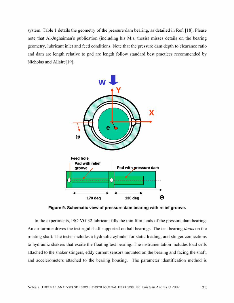
Notes 7. THERMAL ANALYSIS OF FINITE LENGTH JOURNAL BEARINGS. Dr. Luis San Andrés © 2009 22
system. Table 1 details the geometry of the pressure dam bearing, as detailed in Ref. [18]. Please
note that Al-Jughaiman’s publication (including his M.s. thesis) misses details on the bearing
geometry, lubricant inlet and feed conditions. Note that the pressure dam depth to clearance ratio
and dam arc length relative to pad arc length follow standard best practices recommended by
Nicholas and Allaire[19].
X
YW
e
Pad with relief groove Pad with pressure dam
Feed hole
170 deg 130 deg
X
YW
e
Pad with relief groove Pad with pressure dam
Feed hole
170 deg 130 deg
Figure 9. Schematic view of pressure dam bearing with relief groove.
In the experiments, ISO VG 32 lubricant fills the thin film lands of the pressure dam bearing.
An air turbine drives the test rigid shaft supported on ball bearings. The test bearing floats on the
rotating shaft. The tester includes a hydraulic cylinder for static loading, and stinger connections
to hydraulic shakers that excite the floating test bearing. The instrumentation includes load cells
attached to the shaker stingers, eddy current sensors mounted on the bearing and facing the shaft,
and accelerometers attached to the bearing housing. The parameter identification method is

Notes 7. THERMAL ANALYSIS OF FINITE LENGTH JOURNAL BEARINGS. Dr. Luis San Andrés © 2009 23
based on frequency domain measurements and extracts the force coefficients from curve fits of
the real and imaginary parts of the test system impedances.
The maximum load (W) applied equals 12 kN (2,700 lb) which gives a specific pressure
(W/LD) = 13.45 bar (~ 200 psi).
Table 1. Dimensions and operating conditions of pressure dam bearing with relief groove tested by Jughaiman and Childs [18]
Journal diameter D 117.1 mmBearing Length L 76.2 mmRadial clearance c 0.142 mm
pad arc 170 degDam arc length D 130 degwidth (0.75 L) L D 57.1 mm
depth 0.4 mmReilef groove width L R 19.05 mm
depth 0.1 mmLubricant ISO VG 32
Density 860 kg/m3Specific Heat Cp 2000 J/kg-C
Thermal conductivity 0.13 W/m-CViscosity at 45 C 0.028 Pa.s
Visc-temp coefficient 0.034 1/CInlet oil temperature 40-55 ? C
Inlet oil pressure N/A barLoad range 0.1-12 kNSpeed range 4,6,8,10,12 krpm
Closure
Sept 2009: Lecture notes not yet complete. See slide presentation attached.
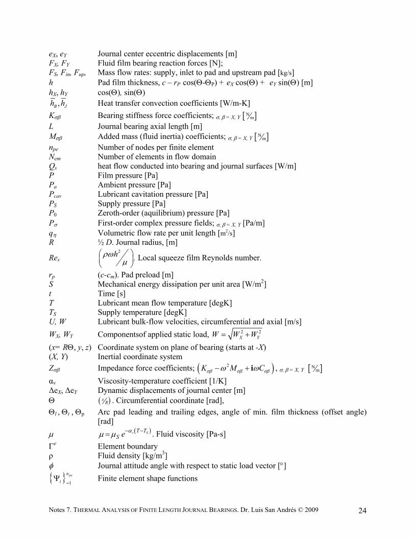
Nomenclature
c Nominal film (pad) clearance [m] cm bearing assembled clearance [m] Cv Lubricant specific heat [J/kg-K] C Bearing damping force coefficients; , = X, Y N s
m
D Journal diameter [m]
Notes 7. THERMAL ANALYSIS OF FINITE LENGTH JOURNAL BEARINGS. Dr. Luis San Andrés © 2009 24
eX, eY Journal center eccentric displacements [m] FX, FY Fluid film bearing reaction forces [N]; FS, Fin, Fup, Mass flow rates: supply, inlet to pad and upstream pad [kg/s]
h Pad film thickness, c – rP cos(-P) + eX cos() + eY sin() [m] hX, hY cos(), sin()
,B Jh h Heat transfer convection coefficients [W/m-K]
K Bearing stiffness force coefficients; , = X, Y Nm
L Journal bearing axial length [m] M Added mass (fluid inertia) coefficients; , = X, Y N
m npe Number of nodes per finite element Nem Number of elements in flow domain Qs heat flow conducted into bearing and journal surfaces [W/m] P Film pressure [Pa] Pa Ambient pressure [Pa] Pcav Lubricant cavitation pressure [Pa] PS Supply pressure [Pa] P0 Zeroth-order (aquilibrium) pressure [Pa] P First-order complex pressure fields; , = X, Y [Pa/m] q Volumetric flow rate per unit length [m2/s] R ½ D. Journal radius, [m]
Res 2h
. Local squeeze film Reynolds number.
rp (c-cm). Pad preload [m] S Mechanical energy dissipation per unit area [W/m2] t Time [s] T Lubricant mean flow temperature [degK] TS Supply temperature [degK] U, W Lubricant bulk-flow velocities, circumferential and axial [m/s]
WX, WY Componentsof applied static load, 2 2X YW W W
(x= R, y, z) Coordinate system on plane of bearing (starts at -X) (X, Y) Inertial coordinate system
Z Impedance force coefficients; 2K M C i , , = X, Y Nm
αv Viscosity-temperature coefficient [1/K] ΔeX, ΔeY Dynamic displacements of journal center [m] x
R . Circumferential coordinate [rad],
l , t , p Arc pad leading and trailing edges, angle of min. film thickness (offset angle) [rad]
v ST TS e . Fluid viscosity [Pa-s]
e Element boundary ρ Fluid density [kg/m3] Journal attitude angle with respect to static load vector []
i
npe
1 Finite element shape functions
Notes 7. THERMAL ANALYSIS OF FINITE LENGTH JOURNAL BEARINGS. Dr. Luis San Andrés © 2009 25
Rotor rotating speed, whirl frequency rad
s
e Finite element sub-domain Subscripts S Supply condition in Inlet to pad n,e,w,s north, east, west and south of control volume N,W,E,S North, east, west and south nodes Superscripts e element
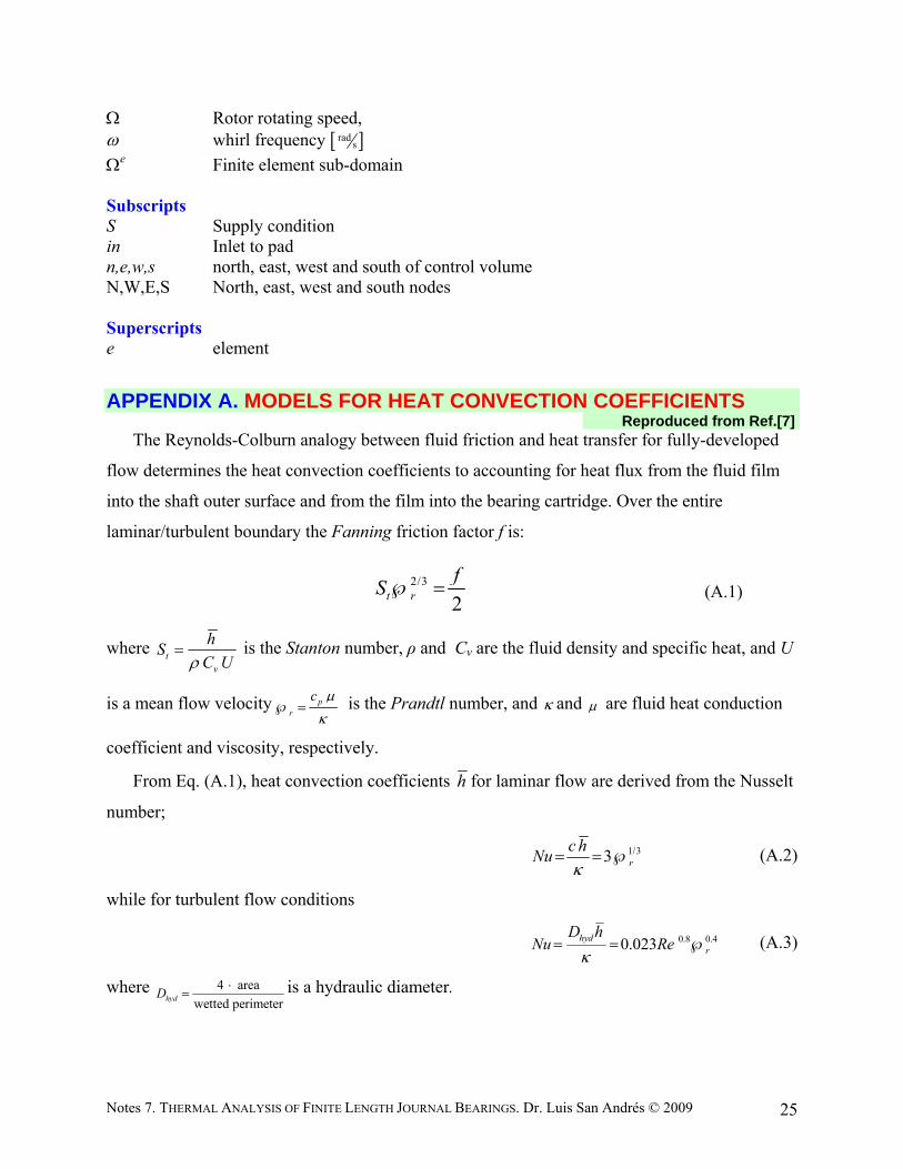
APPENDIX A. MODELS FOR HEAT CONVECTION COEFFICIENTS Reproduced from Ref.[7]
The Reynolds-Colburn analogy between fluid friction and heat transfer for fully-developed
flow determines the heat convection coefficients to accounting for heat flux from the fluid film
into the shaft outer surface and from the film into the bearing cartridge. Over the entire
laminar/turbulent boundary the Fanning friction factor f is:
2/3
2t r
fS (A.1)
where t
v
hS
C U is the Stanton number, ρ and Cv are the fluid density and specific heat, and U
is a mean flow velocity pr
c
is the Prandtl number, and and are fluid heat conduction
coefficient and viscosity, respectively.
From Eq. (A.1), heat convection coefficients h for laminar flow are derived from the Nusselt
number;
1/33 r
c hNu
(A.2)
while for turbulent flow conditions
0.8 0.40.023hydr
D hNu Re
(A.3)
where 4 area
wetted perimeterhydD
is a hydraulic diameter.
Notes 7. THERMAL ANALYSIS OF FINITE LENGTH JOURNAL BEARINGS. Dr. Luis San Andrés © 2009 26
References [1] Boncompain, R., Fillon M., and Frene, J., 1986, "Analysis of Thermal Effects in
Hydrodynamic Bearings", ASME Journal of Tribology, 108 (2), pp. 219-224.
[2] Kucinschi, B., ., Fillon M., Pascovici, M., and Frene, J., 2000, “A Transient Thermoelastohydrodynamic Study of Steadily Loaded Plain Journal Bearings using Finite Element Method Analysis", ASME Journal of Tribology, 122, (1), pp. 219-226, 2000.
[3] Reinhart, F., and Lund, J. W., 1975, "The Influence of Fluid Inertia on the Dynamic Properties of Journal Bearings." ASME J. Lubrication Technology, 97, pp 154-167.
[4] Smith, D. L., 1975, “Journal Bearing Dynamic Characteristics-Effect of Inertia of Lubricant, Proc. Inst. Mech. Engrs., Paper No. 21, 179, Pt.3J, pp 37-44.
[5] San Andrés, L., and Vance, J., 1987, "Effect of Fluid Inertia on Squeeze Film Damper Forces for Small Amplitude Circular Centered Motions," ASLE Transactions, 30, No. 1, pp. 69-76.
[6] San Andrés, L., 2009, Modern Hydrodynamic Lubrication Theory, Notes 10: Thermohydrodynamic Bulk-Flow Model in Thin Film Lubrication, Texas A&M University, http://phn.tamu.edu/me626 [Accessed April 2009]
[7] San Andrés, L., Yang, Z. and Childs, D., 1993, "Thermal Effects in Cryogenic Liquid Annular Seals, I: Theory and Approximate Solutions", ASME Journal of Tribology, 115, 2, pp. 267-276.
[8] San Andrés, L., and Kerth, J., 2004, “Thermal Effects on the Performance of Floating Ring Bearings for Turbochargers”, Journal of Engineering Tribology, Special Issue on Thermal Effects on Fluid Film Lubrication, IMechE Proceedings Part J, 218, pp. 437-450.
[9] San Andrés, L., 2009, Modern Hydrodynamic Lubrication Theory, Notes 6: Cavitation in Liquid Film Bearings, Texas A&M University, http://phn.tamu.edu/me626 [Accessed September 2009]
[10] Pinkus, O., 1990, “Thermal Aspects of Fluid Film Tribology,” ASME Press, N.Y.
[11] Lund, J. W., and E.B. Arwas, 1964, “A Simultaneous Solution of the Lubrication and the Energy Equations for Turbulent Journal Bearing Films,” MTI Report No 64-TR-31, MTI, Inc., N.Y.
[12] Ferron, J., Frene, J., and R. Boncompain, 1983, “A Study of the Thermohydrodynamic Performance of a Plain Journal Bearing Comparison between Theory and Experiments”, ASME Journal of Tribology, Vol. 105, pp. 422-428,
[13] Brito, F.P., Miranda, A.S., Bouter, J., and Fillon, M., Frene, J., and R. Boncompain, 2007, “Experimental investigation on the influence of Supply temperature and Supply Pressure on the Performance of a Two-Axial Groove Hydrodynamic Journal Bearing”, ASME Journal of Tribology, Vol. 129, pp. 98-105.
[14] Lund, J., 1987, “Review of the Concept of Dynamic Coefficients for Fluid Film Journal Bearings,” ASME Journal of Tribology, Vol. 109, pp. 37- 41.
[15] Klit, P. and Lund, J. W., 1988, “Calculation of the Dynamic Coefficients of a Journal Bearing Using a Variational Approach,” ASME Journal of Tribology, Vol. 108, pp. 421 - 425.
Notes 7. THERMAL ANALYSIS OF FINITE LENGTH JOURNAL BEARINGS. Dr. Luis San Andrés © 2009 27
[16] Reddy J. N., Gartling, D. K., 2001, The Finite Element Method in Heat transfer and Fluid Dynamics, CRC Press, Florida, Chap. 2.
[17] Patankar, S.V., 1980, Numerical Heat Transfer and Fluid Flow, Hemisphere Pubs, N.Y.
[18] Al-Jughaiman, and Childs, D., 2007, “Static and Dynamic Characteristics for a Pressure-Dam Bearing”, ASME Paper GT2007-25577.
[19] Nicholas, J., and Allaire, P., 1980, “Analysis of Step Journal Bearings-Finite Length and Stability,” ASLE Transactions, 22, pp. 197-207.
Additional (numerical analyses) references The references below detail numerical analyses for hydrodynamic and hydrostatic liquid and gas bearings, rigid pads and tilting pads. Note that tilting pad bearings show frequency dependent force coefficients. The same holds true for gas bearings Tilting Pad (liquid) bearings San Andrés, L., "Turbulent Flow, Flexure-Pivot Hybrid Bearings for Cryogenic Applications,"
ASME Journal of Tribology, Vol. 118, 1, pp. 190-200, 1996 Gas bearings San Andrés, L., 2006, “Hybrid Flexure Pivot-Tilting Pad Gas Bearings: Analysis and
Experimental Validation,” ASME Journal of Tribology, 128, pp. 551-558.
Delgado, A., L., San Andrés, and J. Justak, 2004, “Analysis of Performance and Rotordynamic Force Coefficients of Brush Seals with Reverse Rotation Ability”, ASME Paper GT 2004-53614
San Andrés, L., and D. Wilde, 2001, “Finite Element Analysis of Gas Bearings for Oil-Free Turbomachinery,” Revue Européenne des Eléments Finis, 10 (6/7), pp. 769-790.
Zirkelback, N., and L. San Andrés, 1999, "Effect of Frequency Excitation on the Force Coefficients of Spiral Groove Thrust Bearings and Face Gas Seals,” ASME Journal of Tribology, 121(4), pp. 853-863.
Foil Gas bearings San Andrés, L., and Kim, T.H., “Thermohydrodynamic Analysis of Bump Type gas Foil
Bearings: A Model Anchored to Test Data” GT2009-59919
San Andrés, L., and Kim, T.H., 2009, “Analysis of Gas Foil Bearings Integrating FE Top Foil Models,” Tribology International, 42(2009), pp. 111-120.
Kim, T.H., and L. San Andrés, 2008, “Heavily Loaded Gas Foil Bearings: a Model Anchored to Test Data,” ASME Journal of Engineering for Gas Turbines and Power, Vol. 130(1), pp. 012504-1-8. (ASME Paper GT 2005-68486).
Kim, T.H., and L. San Andrés, 2006, “Limits for High Speed Operation of Gas Foil Bearings,” ASME Journal of Tribology, 128, pp. 670-673
San Andrés, L., 1995, "Turbulent Flow Foil Bearings for Cryogenic Applications," ASME Journal of Tribology, 117(1), pp. 185-195.

Notes 7. THERMAL ANALYSIS OF FINITE LENGTH JOURNAL BEARINGS. Dr. Luis San Andrés © 2009 28
Hydrostatic/hydrodynamic liquid bearings and seals San Andrés, L., "Thermohydrodynamic Analysis of Fluid Film Bearings for Cryogenic
Applications," AIAA Journal of Propulsion and Power, Vol. 11, 5, pp. 964-972, 1995.
Yang, Z., San Andrés, L. and Childs, D., "Thermal Effects in Cryogenic Liquid Annular Seals, II: Numerical Solution and Results", ASME Journal of Tribology, Vol. 115, 2, pp. 277-284, 1993 (ASME Paper 92-TRIB-5).
San Andrés, L., Yang, Z. and Childs, D., "Thermal Effects in Cryogenic Liquid Annular Seals, I: Theory and Approximate Solutions", ASME Journal of Tribology, Vol. 115, 2, pp. 267-276, 1993 (ASME Paper 92-TRIB-4).
San Andrés, L., "Analysis of Turbulent Hydrostatic Bearings with a Barotropic Fluid," ASME Journal of Tribology, Vol. 114, 4,pp. 755-765,1992.
San Andrés, L., "Fluid Compressibility Effects on the Dynamic Response of Hydrostatic Journal Bearings," WEAR, Vol. 146, pp. 269-283, 1991
San Andrés, L., "Turbulent Hybrid Bearings with Fluid Inertia Effects", ASME Journal of
Tribology, Vol. 112, pp. 699-707,

19
Fortran code : complete – including prediction of inertia force coefficients
GUI (Excel interface) – complete
Examples for calibration:(pressure and temperature fields)oil 360 deg journal bearing
Dowson et al. (1966) Ferron, Frene, Boncompain (1983)Costa, Fillon (2000 2003)
oil two groove journal bearingCosta, Fillon (2000 2003)Brito, Fillon (2006, 2007)
Pressure dam bearingChilds et al (2007, 2008)Load capacity & force
coefficients
Computational code
20
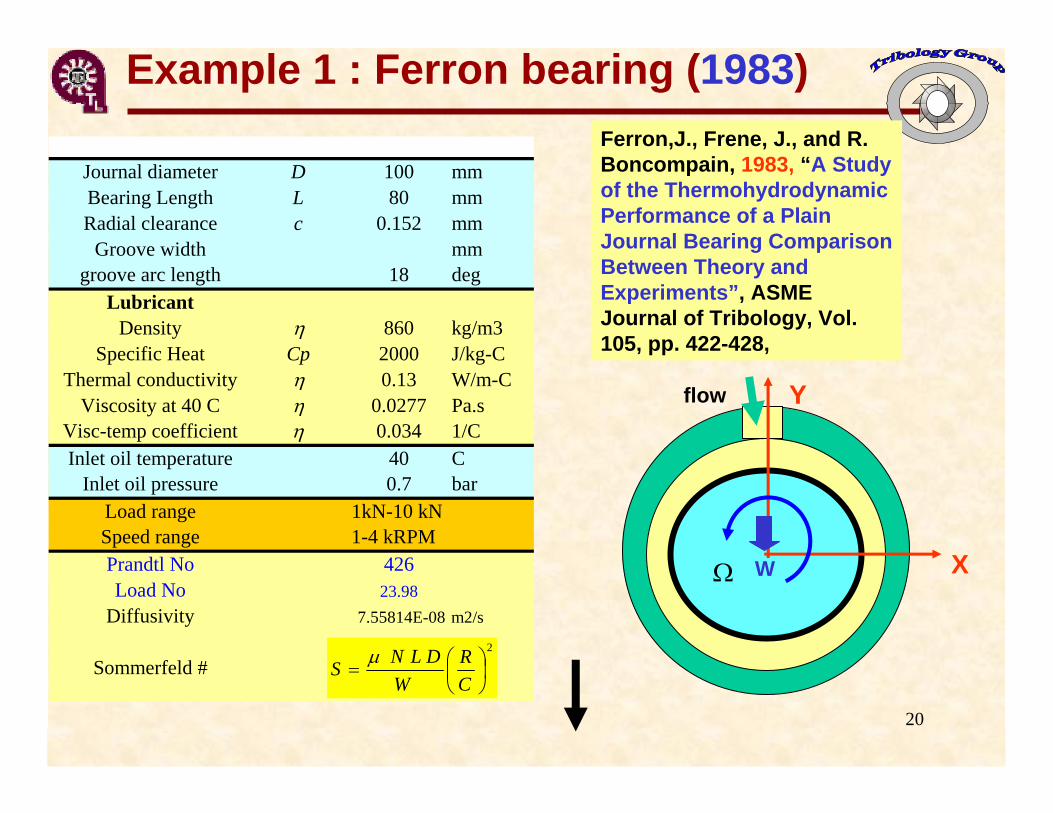
Example 1 : Ferron bearing (1983)
Journal diameter D 100 mmBearing Length L 80 mmRadial clearance c 0.152 mm
Groove width mmgroove arc length 18 deg
LubricantDensity 860 kg/m3
Specific Heat Cp 2000 J/kg-CThermal conductivity 0.13 W/m-C
Viscosity at 40 C 0.0277 Pa.sVisc-temp coefficient 0.034 1/CInlet oil temperature 40 C
Inlet oil pressure 0.7 barLoad range 1kN-10 kNSpeed range 1-4 kRPMPrandtl No 426Load No 23.98
Diffusivity 7.55814E-08 m2/s
Sommerfeld #2
CR
WDLNS
Ferron,J., Frene, J., and R. Boncompain, 1983, “A Study of the Thermohydrodynamic Performance of a Plain Journal Bearing Comparison Between Theory and Experiments”, ASME Journal of Tribology, Vol. 105, pp. 422-428,
X
Yflow
W

21
Ferron et al. bearing (1983)
Pressure and temperature fields – 4 kRPM, 6 kN
Load
Test data
0 30 60 90 120 150 180 210 240 270 300 330 3600
0.5
1
1.5
2pressure
angle (deg)
Pres
sure
(MPa
)
*
0 30 60 90 120 150 180 210 240 270 300 330 36040
42
44
46
48
50temperature
angle (deg)
Tem
pera
ture
(de
g C
)
*
p *
Midplane pressure
Film temperature

22
Ferron et al. bearing (1983)
Eccentricity ratio (e/c) vs Sommerfeld #
Load
Test data
0.0
0.1
0.2
0.3
0.4
0.5
0.6
0.7
0.8
0.9
0.0 0.1 0.2 0.3 0.4 0.5 0.6 0.7 0.8 0.9
Sommerfeld #
ecce
ntric
ity ra
tio
200030004000
RPM
2
CR
WDLNS 2N L D RSW C
23
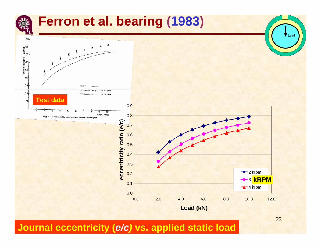
Ferron et al. bearing (1983)
0.0
0.1
0.2
0.3
0.4
0.5
0.6
0.7
0.8
0.9
0.0 2.0 4.0 6.0 8.0 10.0 12.0
Load (kN)
ecce
ntric
ity ra
tio (e
/c)
2 krpm
3 krpm
4 krpmkRPM
Journal eccentricity (e/c) vs. applied static load
Load
Test data
24
Ferron et al. bearing (1983)
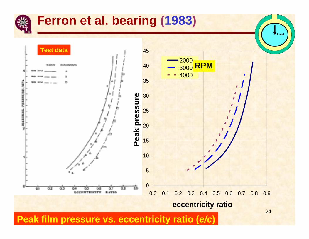
Peak film pressure vs. eccentricity ratio (e/c)
Load
0
5
10
15
20
25
30
35
40
45
0.0 0.1 0.2 0.3 0.4 0.5 0.6 0.7 0.8 0.9
eccentricity ratio
Peak
pre
ssur
e
200030004000
RPM
Test data
25
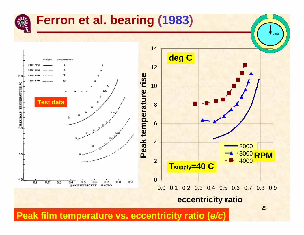
Ferron et al. bearing (1983)
Peak film temperature vs. eccentricity ratio (e/c)
Load
Test data
0
2
4
6
8
10
12
14
0.0 0.1 0.2 0.3 0.4 0.5 0.6 0.7 0.8 0.9
eccentricity ratio
Peak
tem
pera
ture
rise
200030004000
RPM
deg C
Tsupply=40 C
26
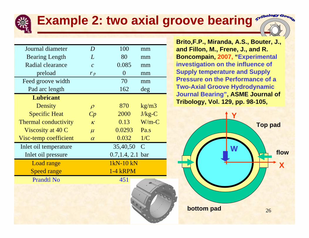
Example 2: two axial groove bearing Brito,F.P., Miranda, A.S., Bouter, J., and Fillon, M., Frene, J., and R. Boncompain, 2007, “Experimental investigation on the influence of Supply temperature and Supply Pressure on the Performance of a Two-Axial Groove Hydrodynamic Journal Bearing”, ASME Journal of Tribology, Vol. 129, pp. 98-105,
Journal diameter D 100 mmBearing Length L 80 mmRadial clearance c 0.085 mm
preload r p 0 mmFeed groove width 70 mm
Pad arc length 162 degLubricant
Density 870 kg/m3Specific Heat Cp 2000 J/kg-C
Thermal conductivity 0.13 W/m-CViscosity at 40 C 0.0293 Pa.s
Visc-temp coefficient 0.032 1/CInlet oil temperature 35,40,50 C
Inlet oil pressure 0.7,1.4, 2.1 barLoad range 1kN-10 kNSpeed range 1-4 kRPMPrandtl No 451
X
Y
W
Top pad
flow
bottom pad
27
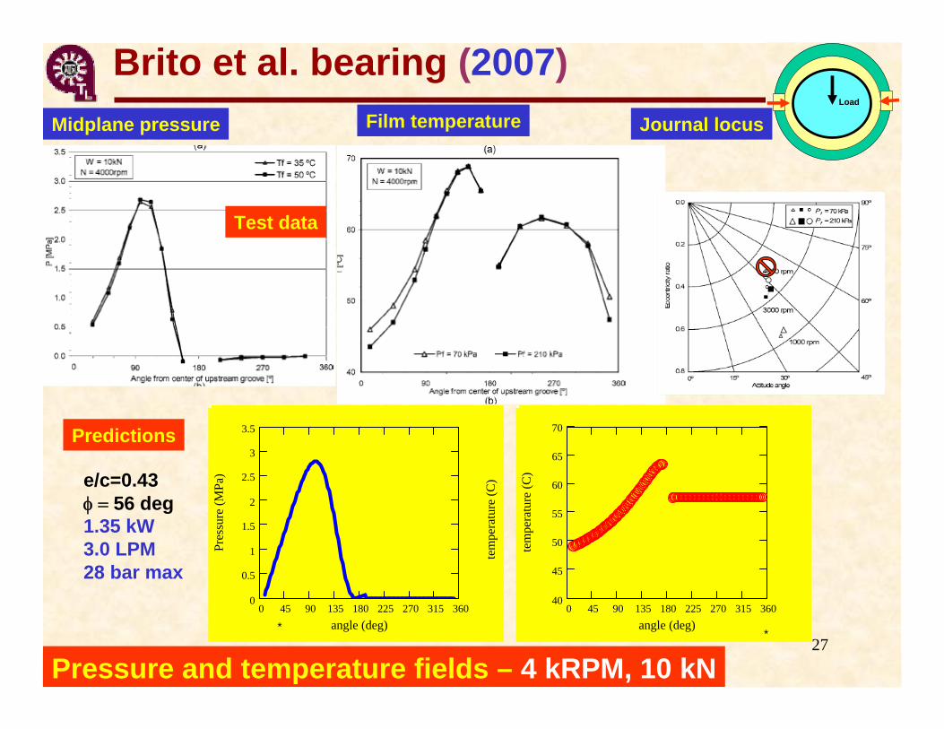
Brito et al. bearing (2007)
Pressure and temperature fields – 4 kRPM, 10 kN
Test data
Midplane pressure Film temperatureLoad
0 45 90 135 180 225 270 315 36040
45
50
55
60
65
70
angle (deg)
tem
pera
ture
(C)
*
Predictions
0 45 90 135 180 225 270 315 3600
0.5
1
1.5
2
2.5
3
3.5
angle (deg)
Pres
sure
(MPa
)
tem
pera
ture
(C)
*
e/c=0.4356 deg1.35 kW3.0 LPM28 bar max
Journal locus

28
Example 3 – Pressure dam bearingAl-Jughaiman, and Childs, D., 2007,“Static and Dynamic Characteristics for a Pressure-Dam Bearing”, ASME Paper GT2007-25577
X
YW
e
Journal diameter D 117.1 mmBearing Length L 76.2 mmRadial clearance c 0.142 mm
pad arc 170 degDam arc length D 130 degwidth (0.75 L) L D 57.1 mm
depth 0.4 mmReilef groove width L R 19.05 mm
depth 0.1 mmLubricant ISO VG 32
Density 860 kg/m3Specific Heat Cp 2000 J/kg-C
Thermal conductivity 0.13 W/m-CViscosity at 45 C 0.028 Pa.s
Visc-temp coefficient 0.034 1/CInlet oil temperature 40-55 ? C
Inlet oil pressure N/A barLoad range 0.1-12 kNSpeed range 4,6,8,10,12 krpm
Missing details on bearing geometry, lubricant and feed conditions. Even with test data at hand, not able to reproduce test results in paper. VERY PECULIAR THERMAL EFFECTS
29
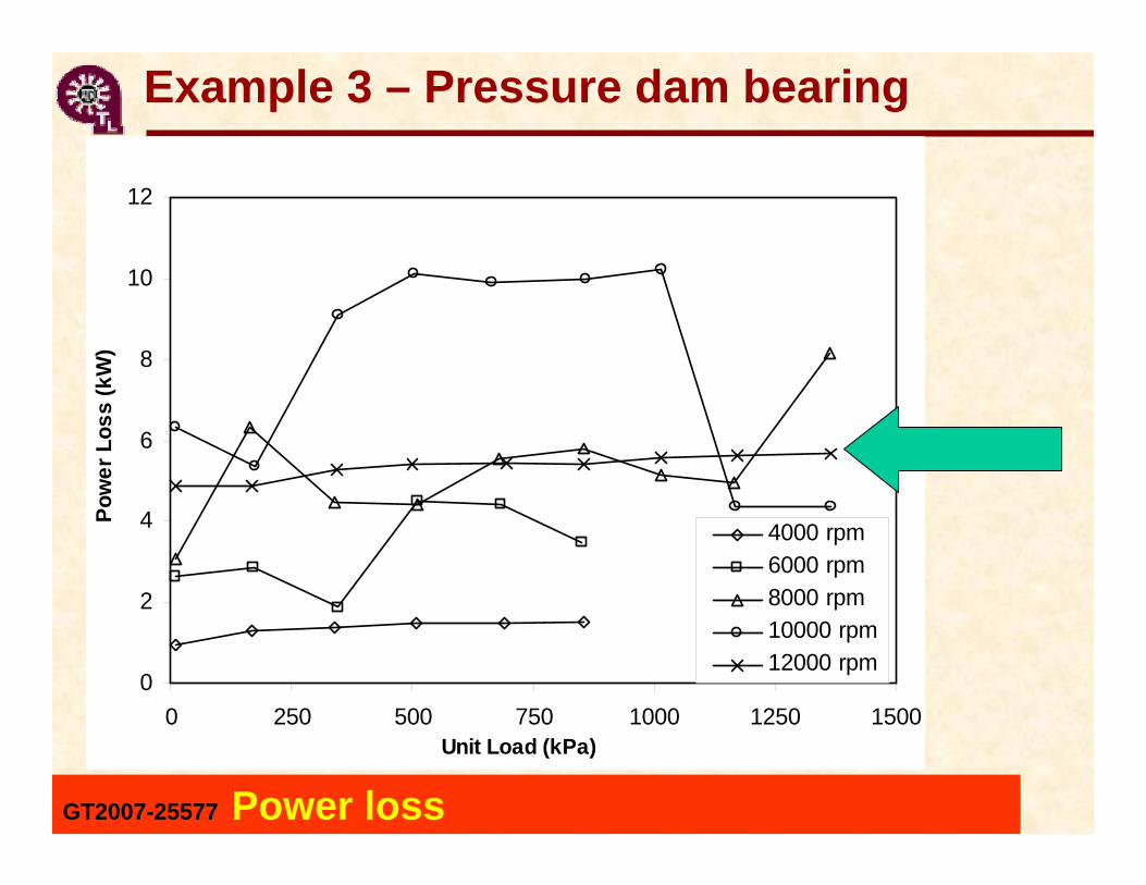
Example 3 – Pressure dam bearing
GT2007-25577 Power loss
0
2
4
6
8
10
12
0 250 500 750 1000 1250 1500Unit Load (kPa)
Pow
er L
oss
(kW
)
4000 rpm6000 rpm8000 rpm10000 rpm12000 rpm

30
0.0
0.1
0.2
0.3
0.4
0.5
0.6
0.7
0.8
0.9
1.0
0 200 400 600 800 1000 1200 1400
Unit Load (W/LD) [kPa]
ecce
ntric
ity ra
tio (e
/c)
4 krpm (pred)10 krpm (pred)4 krpm (test data)10 krpm (test data)12 krpm (pred)test data 12 krpm
TAMU Pressure Dam Bearing with relief track
X
YW
e
Example 3 – Pressure dam bearing
Journal eccentricity vs specific pressure
145 psi
31
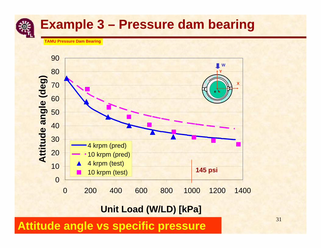
0
10
20
30
40
50
60
70
80
90
0 200 400 600 800 1000 1200 1400
Unit Load (W/LD) [kPa]
Atti
tude
ang
le (d
eg)
4 krpm (pred)10 krpm (pred)4 krpm (test)10 krpm (test)
TAMU Pressure Dam Bearing
X
YW
e
Example 3 – Pressure dam bearing
Attitude angle vs specific pressure
145 psi
32
0
200
400
600
800
1000
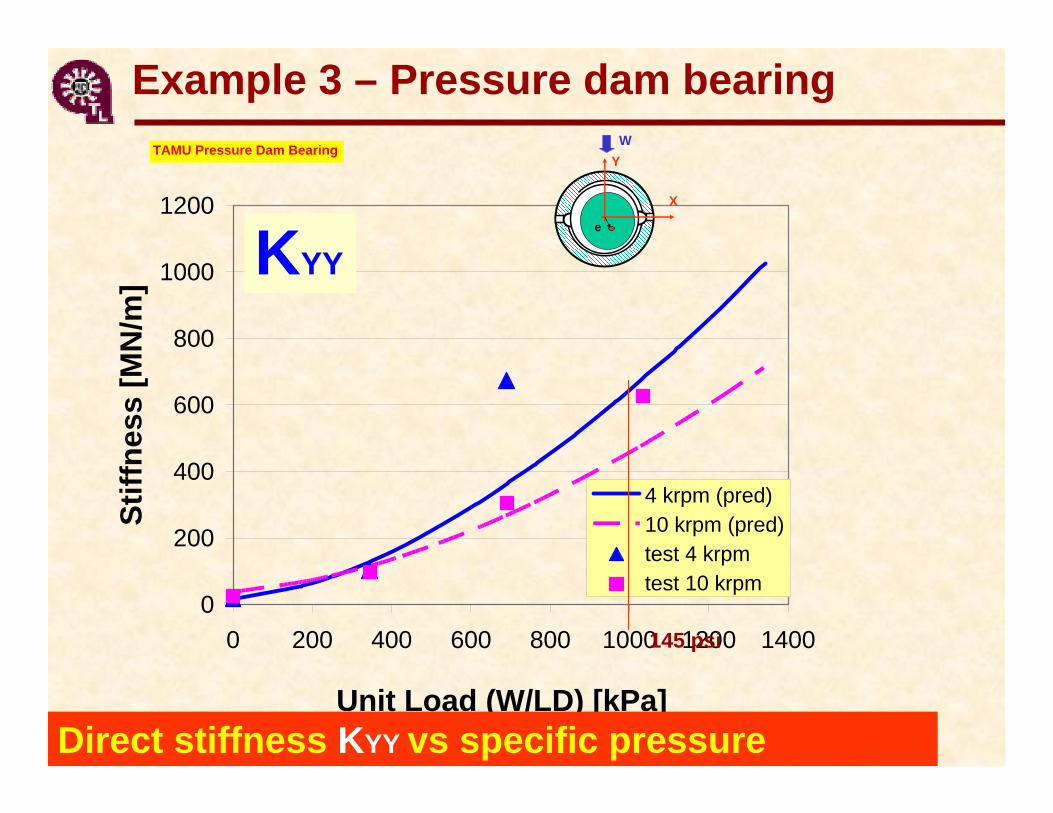
1200
0 200 400 600 800 1000 1200 1400
Unit Load (W/LD) [kPa]
Stiff
ness
[MN
/m]
4 krpm (pred)10 krpm (pred)test 4 krpmtest 10 krpm
TAMU Pressure Dam Bearing
KYY
X
YW
e
Example 3 – Pressure dam bearing
Direct stiffness KYY vs specific pressure
145 psi

33
0
50
100
150
200
250
0 200 400 600 800 1000 1200 1400
Unit Load (W/LD) [kPa]
Stiff
ness
[MN
/m]
4 krpm (pred)10 krpm (pred)4 krpm (test)10 krpm (test)
TAMU Pressure Dam Bearing
KXXX
YW
e
Example 3 – Pressure dam bearing
Direct stiffness KXX vs specific pressure
145 psi

34
-200
20406080
100120140160180
0 200 400 600 800 1000 1200 1400
Unit Load (W/LD) [kPa]
Stiff
ness
[MN
/m]
4 krpm (pred)10 krpm (pred)test 4 krpmtest 10 krpm
TAMU Pressure Dam Bearing with relief track
KXY
X
YW
e
Example 3 – Pressure dam bearing
Cross stiffness KXY vs specific pressure
145 psi

35
0
100
200
300
400
500
600
0 200 400 600 800 1000 1200 1400
Unit Load (W/LD) [kPa]
Stiff
ness
[MN
/m]
4 krpm (pred)10 krpm (pred)test 4 krpmtest 10 krpm
TAMU Pressure Dam Bearing
KYX
X
YW
e
Note: prediction changed sign
Example 3 – Pressure dam bearing
Cross stiffness KYX vs specific pressure
145 psi

36
0
200
400
600
800
1000
1200
1400
1600
1800
2000
0 200 400 600 800 1000 1200 1400
Unit Load (W/LD) [kPa]
Dam
ping
[kN
.s/m
]
4 krpm (pred)10 krpm (pred)test 4 krpmtest 10 krpm
TAMU Pressure Dam Bearing
CYYX
YW
e
Example 3 – Pressure dam bearing
Direct DAMPING CYY vs specific pressure
145 psi
37
0
50
100
150
200
250
300
0 200 400 600 800 1000 1200 1400
Unit Load (W/LD) [kPa]
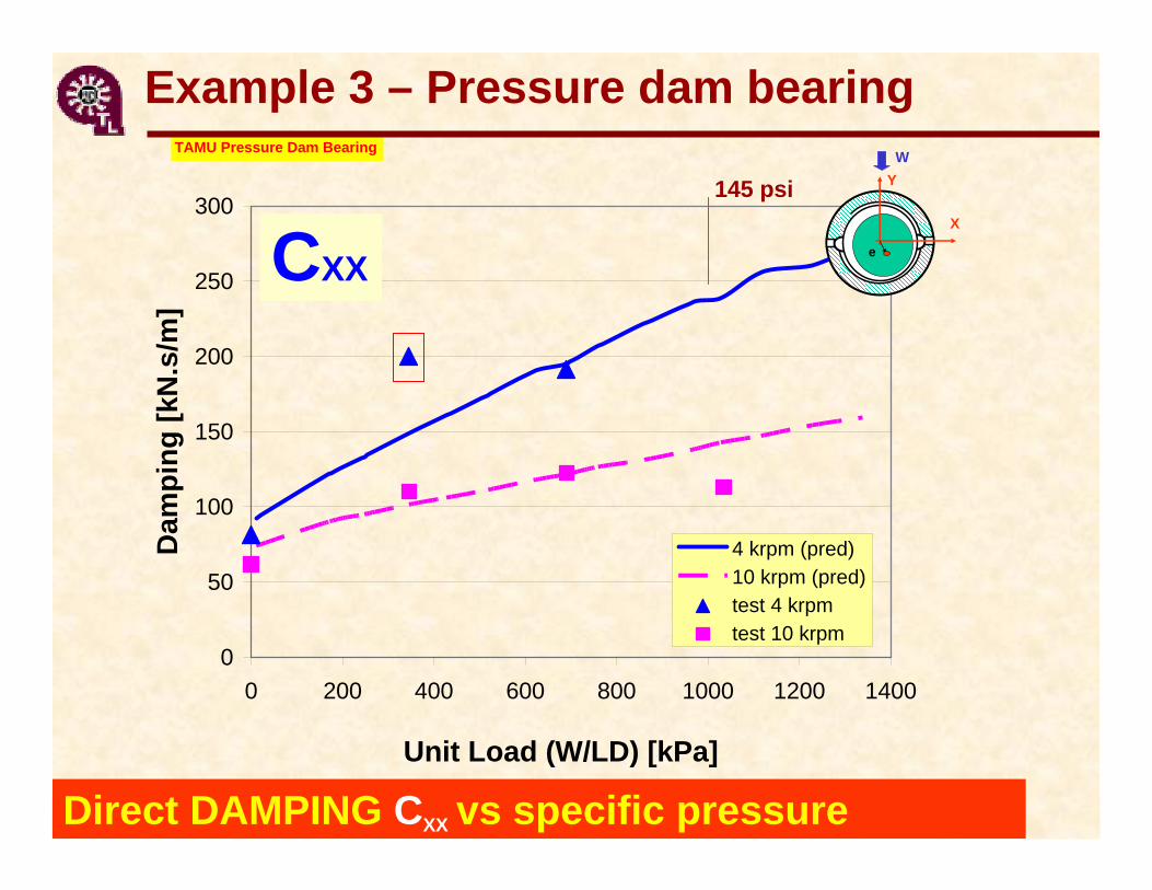
Dam
ping
[kN
.s/m
]
4 krpm (pred)10 krpm (pred)test 4 krpmtest 10 krpm
TAMU Pressure Dam Bearing
CXXX
YW
e
Example 3 – Pressure dam bearing
Direct DAMPING CXX vs specific pressure
145 psi

38
0
100
200
300
400
500
600
0 200 400 600 800 1000 1200 1400
Unit Load (W/LD) [kPa]
Dam
ping
[kN
.s/m
]4 krpm (pred)10 krpm (pred)test 4 krpmtest 10 krpm
TAMU Pressure Dam Bearing
CXYX
YW
e
Example 3 – Pressure dam bearing
Cross DAMPING CXY vs specific pressure
145 psi
39
0
100
200
300
400
500
600
700
0 200 400 600 800 1000 1200 1400
Unit Load (W/LD) [kPa]
Dam
ping
[kN
.s/m
]
4 krpm (pred)10 krpm (pred)test 4 krpmtest 10 krpm
TAMU Pressure Dam Bearing
CYXX
YW
e
Note: prediction changed sign
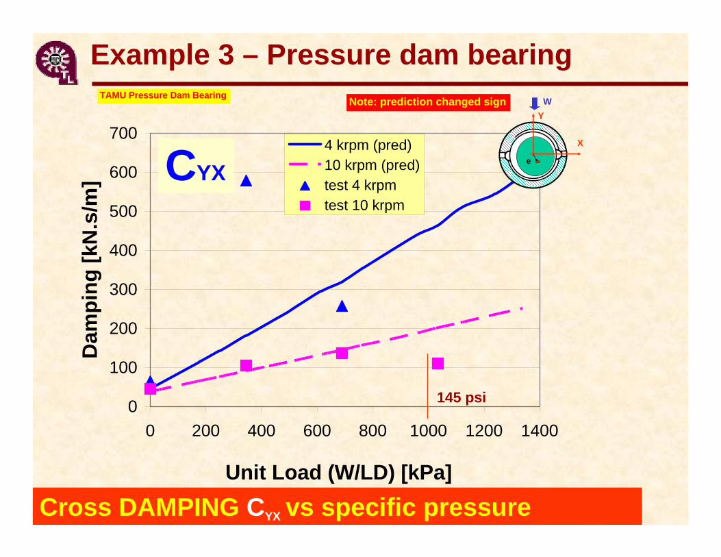
Example 3 – Pressure dam bearing
Cross DAMPING CYX vs specific pressure
145 psi

40
0.00
0.05
0.10
0.15
0.20
0.25
0.30
0.35
0.40
0.45
0.50
0 200 400 600 800 1000 1200 1400
Unit Load (W/LD) [kPa]
Whi
rl fr
eque
ncy
ratio
4 krpm (pred)10 krpm (pred)
TAMU Pressure Dam Bearing
WFR X
YW
e
Example 3 – Pressure dam bearing
Whirl frequency ratio WFR vs specific pressure
41
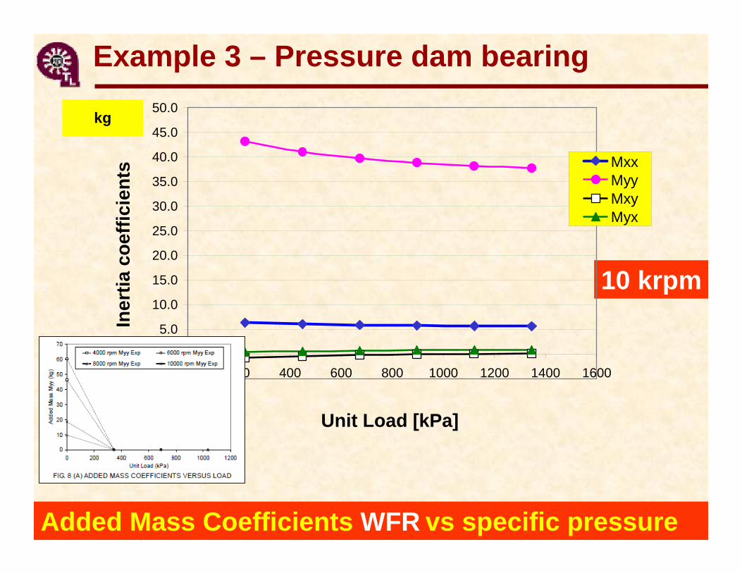
Example 3 – Pressure dam bearing
Added Mass Coefficients WFR vs specific pressure
10 krpm
-5.0
0.0
5.0
10.0
15.0
20.0
25.0
30.0
35.0
40.0
45.0
50.0
0 200 400 600 800 1000 1200 1400 1600
Iner
tia c
oeffi
cien
ts MxxMyyMxyMyx
Unit Load [kPa]
kg