note to users - mcgill universitydigitool.library.mcgill.ca/thesisfile82460.pdf · par...
TRANSCRIPT

NOTE TO USERS
This reproduction is the best copy available.
®
UMI


Modeling and real-time control of sheet reheat phase in
thermoforming
Mark Aj ersch
Department ofElectrical and Computer Engineering Centre for Intelligent Machines - Systems and Control Group
Industrial Automation Lab McGill University, Montreal, Canada
August 2004
A thesis submitted to McGill University in partial fulfillment of the requirements of a Masters degree in Electrical and Computer Engineering
© Mark Ajersch 2004

1+1 Library and Archives Canada
Bibliothèque et Archives Canada
Published Heritage Branch
Direction du Patrimoine de l'édition
395 Wellington Street Ottawa ON K1A ON4 Canada
395, rue Wellington Ottawa ON K1A ON4 Canada
NOTICE: The author has granted a nonexclusive license allowing Library and Archives Canada to reproduce, publish, archive, preserve, conserve, communicate to the public by telecommunication or on the Internet, loan, distribute and sell th es es worldwide, for commercial or noncommercial purposes, in microform, paper, electronic and/or any other formats.
The author retains copyright ownership and moral rights in this thesis. Neither the thesis nor substantial extracts from it may be printed or otherwise reproduced without the author's permission.
ln compliance with the Canadian Privacy Act some supporting forms may have been removed from this thesis.
While these forms may be included in the document page count, their removal does not represent any loss of content from the thesis.
• •• Canada
AVIS:
Your file Votre référence ISBN: 0-494-12575-6 Our file Notre référence ISBN: 0-494-12575-6
L'auteur a accordé une licence non exclusive permettant à la Bibliothèque et Archives Canada de reproduire, publier, archiver, sauvegarder, conserver, transmettre au public par télécommunication ou par l'Internet, prêter, distribuer et vendre des thèses partout dans le monde, à des fins commerciales ou autres, sur support microforme, papier, électronique et/ou autres formats.
L'auteur conserve la propriété du droit d'auteur et des droits moraux qui protège cette thèse. Ni la thèse ni des extraits substantiels de celle-ci ne doivent être imprimés ou autrement reproduits sans son autorisation.
Conformément à la loi canadienne sur la protection de la vie privée, quelques formulaires secondaires ont été enlevés de cette thèse.
Bien que ces formulaires aient inclus dans la pagination, il n'y aura aucun contenu manquant.

Abstract
The heating, or sheet reheat, phase in thennofonning is the focus of this work. The first
objective is to develop a reliable state-space model ofthis process for simulation analysis.
The second objective is to develop a simple linear real-time in-cycle controller for the
sheet reheat phase. This controller will improve part quality, decrease energy
expenditures and machine wear, and optimize heating time by assuring a desired sheet
temperature distribution. The final result is a reduction in production cost per part for the
thennofonning industry.
A sheet model is developed from first princip les, and improved through the addition of
energy absorption tenns. The sheet model is tested against experimental results, giving
errors of less than 5°C over the entire transient temperature curve at different depths after
tuning.
A linearization assumption is made, and a two-Ioop control algorithm is designed for the
sheet surface temperatures. These temperatures are monitored using infrared sensors at
different locations on the sheet. Simple PI controllers are used in real-time to monitor and
maintain these IR sensors about a given step or ramp input, with great precision (less than
1°C error).
11

Résumé
Ce travail traite de la commande automatique en temps réel du procédé de chauffage
d'une feuille de polymère pour le thermoformage. Le système de commande améliorera
la qualité de la pièce formée, diminuera les coûts d'énergie et de maintien d'équipement,
et optimisera le temps de chauffage en assurant une distribution de température désirée
sur la feuille. Les coûts de production par pièce thermoformée seront réduits.
Un modèle de la feuille est developpé à partir des lois physiques, et est amélioré par
l'inclusion de l'absorption d'énergie radiante à l'intérieur de la feuille. Ce modèle est
validé par des résultats expérimentaux, donnant des erreurs de simulation d'environ 5°C
sur les courbes transitoires de température à plusieurs profondeurs différentes.
À partir d'une hypothèse de linéarisation, l'algorithme de commande est défini en deux
boucles. Des capteurs infrarouges mesurent les températures de surface de la feuille à des
endroits différents. En temps réel, un compensateur PI maintient chacune de ces mesures
de température avec une excellente précision (moins de lOC d'erreur), que la sortie
désirée soit une rampe ou un échelon.
111
Acknowledgements
l would primarily like to thank Prof essor Benoit Boulet for his guidance and thought
provoking analysis, throughout the duration of my work at Mc Gill. l greatly appreciate
his technical and financial help.
l have also benefited from the expenence and attitude of Arnmar Haurani and Guy
Gauthier. Many interesting ideas and experiments were conceived during our group
discussions, and carried out with their help.
l must also acknowledge the immense contributions from CNRC-NRC IMI. All
experimental material, from the therrnoforrning oven and plastic sheets to the FEM
forrning and real-time software programs, was provided by IMI, and enabled me to
complete this thesis. The guidance and experience of Robert Di Raddo was especially
appreciated. Benoit Lanctot and Linda Pecora were excellent tutors in the usage of the
FORMSIM software. Christian de Grandpré and Marc-André Rainville were also
extremely helpful with experimental setups and were always available to answer
questions.
Finally, l would like to thank my family and friends for their continued support.
IV

Table of Contents
ABSTRACT .......................................................................................................... Il RÉSUMÉ ............................................................................................................. 111 ACKNOWLEDGEMENTS .................................................................................... 1V TABLE OF CONTENTS ....................................................................................... V LIST OF FIGURES ............................................................................................ Vlll LIST OF TABLES ................................................................................................ IX
CHAPTER 1 INTRODUCTION ......................................................................... - 1 -
1.1 Thesis Objective ................................................................................................................................... - 1 -
1.1.1 Benefits to Industry ...................................................................................................................... - 2 -
1.2 Literature review .................................................................................................................................. - 3 -
1.2.1 Thermoforrning models ................................................................................................................ - 3 -1.2.2 IR sensors ..................................................................................................................................... - 5 -1.2.3 Industrial applications of real-time controL ................................................................................ - 5 -
CHAPTER 2 THERMOFORMING .................................................................... - 7 -
2.1 History .................................................................................................................................................. - 7 -2.2 Markets ................................................................................................................................................. - 9 -2.3 Sheet gage .......................................................................................................................................... - Il -2.4 Process Description ............................................................................................................................ - Il -
2.4.1 Clamping .................................................................................................................................... - Il -2.4.2 Heating ....................................................................................................................................... - 12 -
2.4.2.1 Heat Sources ....................................................................................................................... - 13 -
2.4.3 Forrning ...................................................................................................................................... - 13 -2.4.4 Trimming .................................................................................................................................... - 15 -
2.5 SheetReheatphase ............................................................................................................................. - 15-
2.5.1 Zoned Heating ............................................................................................................................ - 17 -
CHAPTER 3 MODELING THE SHEET-HEATER SYSTEM ........................... - 18-
3.1 Heat Transfer Basics .......................................................................................................................... - 18 -
3.1.1 Conduction ................................................................................................................................. - 18 -3 .1.2 Convection .................................................................................................................................. - 21 -3.1.3 Radiation .................................................................................................................................... - 23 -
3.1.3.1 Emissivity ..................................... : ..................................................................................... - 23 -
3.1.3 .1.1 Heating Element Emissivity CaIculations ................................................................... - 26 -
3.1.3.2 View Factors ....................................................................................................................... - 30 -
3.2 Plastic Sheet Modeling - Energy Absorption within the Sheet... ....................................................... - 31 -
3.2.1 Moore Model of Plastic Sheet .................................................................................................... - 32 -3.2.2 Energy Absorption within the sheet ........................................................................................... - 35 -
v

3.3 Complete Heater-Sheet State-Space Model ....................................................................................... - 38 -
3.3.1 Definitions .................................................................................................................................. - 38 -3.3.2 State equations ............................................................................................................................ - 39 -3.3.3 Model Validation ........................................................................................................................ - 42-
3.3.3.1 Testsetup ............................................................................................................................ -42-3.3.3.2 Experimental results ........................................................................................................... - 44 -3.3.3.3 Reasons for errOL ................................................................................................................ - 52 -
CHAPTER 4 REAL-TIME CONTROL OF AAA THERMOFORMING OVEN .. - 56 -
4.1 AAA Machine Overview .................................................................................................................... - 57 -
4.1.1 System Actuators and Layout.. ................................................................................................... - 58 -4.1.2 Existing Control Structure .......................................................................................................... - 60 -
4.1.2.1 Modeling the actuators ........................................................................................................ - 62 -
4.1.2.1.1 Test setup .................................................................................................................... - 63-4.1.2.1.2 Experimental results .................................................................................................... - 64 -
4.1.2.2 Actuator Heating/Cooling Rate ........................................................................................... - 67 -
4.1.3 Infrared Sensors .......................................................................................................................... - 68 -
4.1.3.1 Distance to Spot Ratio ........................................................................................................ - 70 -4.1.3.2 IR Sensor Locations ............................................................................................................ - 71 -
4.1.4 OPAL-RT RT -LAB Operating System ...................................................................................... - 72 -
4.1.4.1 RT -LAB system structure ................................................................................................... - 72 -
4.1.4.1.1 System Inputs .............................................................................................................. - 74 -4.1.4.1.2 System Outputs ........................................................................................................... - 76 -
4.2 Real-Time Control of Sheet Temperatures ......................................................................................... - 76-
4.2.1 Linearizing the sheet reheat system ............................................................................................ - 77 -4.2.2 Control algorithm: multilayer controL ...................................................................................... - 81 -4.2.3 Inner loop Control: Embedded Heating Element Temperatures ................................................. - 83 -
4.2.3.1 Hybrid Feedforward-PID controller ................................................................................... - 84 -4.2.3.2 On-off or Bang-Bang ControL ........................................................................................... - 93 -
4.2.4 Outer loop Control: Sheet Surface Temperatures using IR ........................................................ - 95 -
4.2.4.1 IR sensor output conditioning ............................................................................................. - 95 -4.2.4.2 Steady-state relationship between heaters and sheet.. ......................................................... - 96 -
4.2.4.2.1 Insulator sheet ............................................................................................................. - 96 -4.2.4.2.2 Test Setup .................................................................................................................... - 97 -4.2.4.2.3 Experimental Results " ................................................................................................ - 98 -4.2.4.2.4 Pseudo-inverse .......................................................................................................... - 100 -
4.2.4.3 Steady-State Control of Sheet Temperatures .................................................................... - 100 -
4.2.4.3.1 Transient Sheet Surface Temperature Responses ..................................................... - 101 -4.2.4.3.2 Model and Controller ................................................................................................ - 103 -4.2.4.3.3 Real-Time implementation ........................................................................................ - 104-
4.2.4.4 Ramp Input Control .......................................................................................................... - 107 -
CHAPTER 5 CONCLUSION ........................................................................ - 111 -
5.1 Summary .......................................................................................................................................... - 111 -
VI
5.2 Recommendations and Future Work ................................................................................................ - 112 -
CHAPTER 6 REFERENCES ........................................................................ - 114-APPENDIX A: LIST OF POL yMERS ............................................................ - 118 -APPENDIX B: D-M-E INSUlATOR SHEET SPECIFICATIONS .................. - 119-APPENDIX C: NON-L1NEAR MODEl MATlAB CODE ............................... - 120-
Vll

List of Figures
Figure 2-1: Drape forrning (before and after) ........................................................................................... - 13 -Figure 2-2: Vacuum or Pressure forming ................................................................................................. - 14 -Figure 2-3: Temperature forrning window for material X [17] ................................................................ - 16 -Figure 2-4: Temperature distribution across sheet thickness ................................................................... - 16 -Figure 3-1: Closed Oven used in heating element emissivity calculations .............................................. - 27 -Figure 3-2: Steady-State Temperature Curves at 350C Setpoint .............................................................. - 30 -Figure 3-3: Radiation ray tracing between finite paraUe1 plate elements [10] ......................................... - 30 -Figure 3-4: Plastic Sheet Discretization ................................................................................................... - 32 -Figure 3-5: Start of Heating Curves for 12mm sheet at 280C .................................................................. - 34-Figure 3-6: Test Setup for Thick Sheet Experiments ............................................................................... - 43 -Figure 3-7: 280C Experimental Temperature Curves .............................................................................. - 45 -Figure 3-8: 280C Simulation Model Temperature Curves ....................................................................... - 46 -Figure 3-9: 280C Simulation Error (vs. Experimental Data) ................................................................... - 46 -Figure 3-10: 320C Experimental Temperature Curves ............................................................................ - 47 -Figure 3-11: 320C Simulated Model Temperature Curves ...................................................................... - 48 -Figure 3-12: 320C Simulation Error (vs. Experimental Data) ................................................................. - 48-Figure 3-13: 420C Experimental Temperature Curves ............................................................................ - 49 -Figure 3-14: 420C Simulated Model Temperature Curves ...................................................................... - 50 -Figure 3-15: 420C Simulation Error (vs. Experimental Data) ................................................................. - 50 -Figure 3-16: IR temperature measurement ofHeating Element Surfaee (setpoint 300C) ........................ - 54-Figure 3-17: LlOI data line from IR Camera picture above (setpoint 300C) ........................................... - 54 -Figure 3-18: Histogram showing temperature distribution along line LlOl ............................................. - 55 -Figure 4-1: AAA Thermoforming machine (front view) ......................................................................... - 58-Figure 4-2: Tempco 650W Heating element.. .......................................................................................... - 59-Figure 4-3: Lower Heating tray ................................................................................................................ - 59 -Figure 4-4: Top view of AAA Oven ........................................................................................................ - 60 -Figure 4-5: PID control panel (for a1l12 heater zones) ............................................................................ - 61 -Figure 4-6: PID Control Loop .................................................................................................................. - 62 -Figure 4-7: B2 Embedded Thermocouple Temperature - 10% Dut Y Cycle ............................................ - 64 -Figure 4-8: Closed-Loop PID model vs. Actual data ............................................................................... - 66-Figure 4-9: B2 Heating (100%) and Cooling (free) Curves ..................................................................... - 67 -Figure 4-10: Raytek Thermalert® MIC™ IR sensor with coolingjacket.. .............................................. - 70-Figure 4-11: Examples of different D : S ratios ...................................................................................... - 70 -Figure 4-12: Top view of AAA oyen with IR sensors ............................................................................. - 71 -Figure 4-13: RT-LAB Hardware Package ................................................................................................ - 73 -Figure 4-14: Thermocouple signal conditioners from Analog Devices (3B37, 3B47) ............................. - 75 -Figure 4-15: Linearization function about 160°C setpoint (for HDPE) ................................................... - 79 -Figure 4-16: Percent error for Linearization over entire HDPE forrning range (140-180°C) .................. - 79-Figure 4-17: Linearization function for 350C setpoint ............................................................................. - 80-Figure 4-18: Percent Error for linearization over heating element active range (300-400°C) ................. - 81 -Figure 4-19: Inner Loop Heating Element Control Schematic ................................................................. - 82 -Figure 4-20: Outer Loop ControUer Block Diagram ................................................................................ - 82 -Figure 4-21: Signal input from Analog Deviees 3B37 Signal Conditioner .............................................. - 84 -Figure 4-22: Signal input from Analog Devices 3B47 Signal Conditioner. ............................................. - 84 -Figure 4-23: Filtered and Unfiltered embedded thermocouple signaL .................................................... - 86 -Figure 4-24: Signal delay due to low pass filter ....................................................................................... - 87 -Figure 4-25: Hybrid Feedforward PID controUer. .................................................................................... - 88 -Figure 4-26: Square Wave Function ........................................................................................................ - 89 -Figure 4-27: Embedded Thermocouple reaction to various PID setpoints (zone B1) .............................. - 90-Figure 4-28: Cross section of eeramic heating element... ......................................................................... - 91 -Figure 4-29: Ceramic Heating element Conduction Delay (Heating Zone B2) ....................................... - 92 -
Vlll

Figure 4-30: Block Diagram of Bang-Bang Inner Loop ControIler ......................................................... - 93 -Figure 4-31: Conduction Delay Oscillations for Bang-Bang ControUer (zone BI) ................................. - 94 -Figure 4-32: Signal conditioning of the IR output signal ......................................................................... - 96 -Figure 4-33: Transient Sheet Surface Temperature Responses .............................................................. - 101 -Figure 4-34: First-Order fit ofIR sensor responses to 150°C step on aIl zones ..................................... - 102 -Figure 4-35: Simulink Model of SheetlHeater system ........................................................................... - 103 -Figure 4-36: Simulated PI Control response to step IIP of[175 150125 100] ...................................... - 104-Figure 4-37: Open-Ioop Control ofIR Measurements (nominal setpoint) ............................................. - 105 -Figure 4-38: Closed-Loop Control ofIR Measurements (nominal setpoint) ......................................... - 106-Figure 4-39: Embedded Thermocouple Heater Temperatures (aIl zones) .............................................. - 107 -Figure 4-40: Velocity Feedforward PI controIler for Ramp input .......................................................... - 108 -Figure 4-41: IRTl Sens or Response to Ramp input ............................................................................... - 109 -Figure 4-42: IRTl Sensor Error for Ramp Input .................................................................................... - 109 -Figure 4-43: Heating Element Response to Ramp Input.. ...................................................................... - 110-
List of Tables
Table 2-1: US Polymers Converted via Thermoforrning ........................................................................... - 9 -Table 2-2: Major Thermoforrning Industries and their products [1 0] ...................................................... - 10-Table 3-1: Material Thermal Conductivity Ranges .................................................................................. - 20 -Table 3-2: Range in Values for Convection Heat Transfer Coefficient [10] ............................................ - 22-Table 3-3: Emissivity of certain materials [18] ........................................................................................ - 25 -Table 3-4: Experimental Heating Element Emissivity Results ................................................................ - 29 -Table 3-5: Tuned Simulation Parameters for 280C, 320C and 420C tests ............................................... - 51 -Table 4-1: B2 parameters for several dut y cycles .................................................................................... - 65 -Table 4-2: Heating and Cooling Rates for zone B2 .................................................................................. - 68 -Table 4-3: Open-Loop Insulator Sheet Step testing results ...................................................................... - 98 -
IX

Chapter 1 Introduction
1. 1 Thesis Objective
Thermoforming is an industrial process in which plastic sheets are heated and then
formed into useful parts. It can be divided into three distinct phases: heating, forming and
cooling. The sheet is heated in an oyen until it becomes pliable. The softened sheet is
then formed over the mold and cooled until it hardens. A more detailed description of the
thermoforming process is found in the following chapter.
The heating, or sheet reheat, phase is the focus of this work. The first objective is to
develop a reliable state-space model of this process for simulation analysis. The second
objective is to develop a simple linear real-time in-cycle controller for the sheet reheat
phase. There are two different control strategies for this type of system, in-cycle and
cycle-to-cycle. A cycle-to-cycle controller by definition only takes an action after the
whole cycle has been completed, i.e., the part has been formed, in order to improve the
next part. The in-cycle controller, however, reacts while the part is being heated, so that a
desired sheet temperature profile can be attained in an optimal heating time.
Bach of these objectives has separate benefits. The non-linear state-space mode1 can be
used off-line in order to determine the optimal system parameters. Once the system
parameters have been found, the desired forming time and temperature distribution
profile for a typical part can be quickly estimated from the model output. The
temperature distribution can then be achieved using the simple real-time in-cycle
controller, ensuring a satisfactorily formed part at the machine output.
- 1 -

At present, the industry standard is an open-Ioop control system, where the machine
operator "tweaks" the oven temperatures until a satisfactory part is made. At this point
these settings are maintained until machine drift or other factors cause the final parts to
become unsatisfactory, whereupon the operator will readjust the settings. Using the
model, the operator can first determine the machine parameters, and obtain a temperature
distribution, either across the sheet surface, or even within the sheet. Then the operator
will only have to input this desired temperature profile for the final part. The in-cycle
controller will then determine the oven temperature settings that will reach this profile in
the shortest possible time.
1.1.1 Benefits ta Industry
The development of such a controller will benefit the thermoforming industry in several
different ways.
The quality of the part will improve, on average, due to the better energy distribution
within the sheet. AIso, this even temperature distribution can lead to less rejected parts, a
major benefit to the thermoforming industries that make the larger, higher-end, more
expensive parts (gas tanks, for instance).The material cost per part will then decrease.
Similarly, the time needed to produce a sheet with the desired temperature distribution
will be optimized. Using the sheet reheat model, the optimal heating trajectories can be
determined, shortening the heating time, and increasing the number of parts that can be
produced per shift and, consequently, the machine throughput as weIl.
Other benefits to industry derived from this controller include the minimization of the
energy input to the thermoforming oven. By controlling the energy entering the sheet, an
- 2 -

optimal oven temperature setting can be determined in order to lower the heating costs.
The machine itself may also require less maintenance and repair work. Heating elements
become less efficient as they age, and the controller will compensate for this loss of
efficiency by directing the adjoining elements to heat more.
The end result of all of these benefits is a decrease in production cost per part, an
important savings for the thermoforming industry.
1.2 Literature review
Interesting technological advances have been put forward in most polymer processes,
especially extrusion blow molding and injection molding. Less work has been done in the
thermoforming industry, but a large number of interesting articles have been published in
the last five years. Most of these are re1ated to the development of sheet models during
the reheat phase, but sorne work has also been done modeling the heating elements as
well. Only one paper was found that discussed cycle-to-cycle control in thermoforming.
Michaeli and van Marwick [19] proposed a two-level controller to monitor the
distribution of the wall thickness in thermoformed parts, and suggested two methods of
measuring this property on-line, either using ultrasound sensors, or by triangulation laser.
1.2.1 Thermoforming models
Smaller sheet models can be used on-line to determine the time-varying temperatures
within the sheet as it is being heated. The initial work in mode1ing the sheet reheat phase
of thermoforming for thick sheets was done by Moore et al. [16,17], who proposed a
discretization of the sheet across its thickness. Moore developed simulated H-infinity and
- 3 -

model-predictive in-cycle controllers for this sheet model as weIl. Duarte and Covas [4,5]
investigated the inverse heating problem for a roll-fed (or thin sheet) thermoforming
machine. They developed another model determining ideal heating element temperatures
to give a uniform sheet surface temperature. This model included energy absorption
within the sheet according to the Beer-Lambert law. Two differing solutions were
proposed, and a sensitivity analysis involving parameter perturbation was performed.
Monteix et al. [6] also developed a control-volume method for determining radiant heat
transfer within the plastic sheet. Their model also included one-dimensional energy
absorption due to Beer-Lambert Law.
Larger finite-element models (FEM) of the thermoforming process are used in simulation
in order to pre-determine optimal operating conditions for precise sheet thickness
distribution during thermoforming. The first such computer-aided model was developed
by Throne [1], who investigated the effects of zoned heating and changes in heater-sheet
distance on the sheet surface temperatures. Y ousefi et al. [3] improved FEM modeling of
reheat phase in thermoforming due to uncertainty treatment of several machine
parameters. DiRaddo et al. [23] examined the effects of machine drift by comparing
experimental results to the FEM model. Other FEM models include those developed by
Sala et al. [20], a numerical solution based on physical testing of polymer parameters and
tested experimentally against the forming of a low-temperature refrigerator cell.
The sheet itself is not the only aspect of the thermoforming oyen that has been modeled.
Much work has been done discussing the heating elements that provide energy to the
sheet. Schmidt et al. [8] characterized the spectral responses of several different types of
heating elements, discovering that halogen heating elements were more efficient than
- 4 -

their ceramic or quartz counterparts. Petterson and Stenstrom [22] developed a steady
state and transient model of an electric IR heater, as applied to a paper dryer (for the pulp
and paper industry).
1.2.2 IR sensors
Several researchers investigated the measurement validity and accuracy of infrared
temperature sensors, similar to those used to measure sheet surface temperatures inside a
thermoforming oyen. Lappin and Martin [2] first discussed the implementation of these
sensors on a thermoforming machine, as weIl as potential calibration and noise issues.
Bugbee et al. [7] characterized three different types of IR sensors, according to
calibration and sensor body temperature errors. A new approach to the calibration of IR
thermometers was proposed and prototyped by Baker et al. [9]
1.2.3 Industrial applications of real-time control
Real-time process control has not yet been applied in thermoforming. However, in other
industries, much work has been done to develop models that will achieve this objective.
Safarty et al. [21] applied advanced process control to the semi-conductor industry,
developing a method of wafer-to-wafer testing to improve throughput and flexibility of
the manufacturing process. Using trained neural networks and machine vision algorithms,
Peng et al. [25] developed an intelligent approach for optimizing robot arc welding in
real-time. Finally, Hossain and Suyut [24] successfully integrated a dynamic statistical
process control model with a real-time industrial process.
- 5 -

In Chapter 2, thermoforming is described in more detail. The sheet model is developed
from first princip les and then tested against experimental results in Chapter 3. Chapter 4
includes a description of the experimental real-time setup, as well as the first real-time in
cycle sheet surface temperature controllers developed for sheet reheat. The final chapter
contains a brief summary, and offers potential model-based real-time control solutions
combining the twin objectives ofthis work: the absorption model from Chapter 3 and the
real-time controllers from Chapter 4.
- 6-

Chapter 2 Thermoforming
Thennofonning is a generic tenn describing the many techniques for producing useful
plastic parts from a fiat sheet. In its simplest fonn, thennofonning is the draping of a
heated (and softened) plastic sheet over a mold.
This chapter first gives a brief history of thennofonning, before listing examples of
thennofonned parts. AIl phases of the process are then described in small detail, with
special emphasis on the sheet reheat phase and zoned heating as they relate to the
development of an in-cycle controller.
2.1 History
Thennofonning, in one fonn or another, has been around for many centuries. The earliest
civilizations in Egypt and Micronesia heated tortoise shells in hot oil. The keratin within
the shell was then cooled and shaped to fonn food containers and bowls. In the Americas,
the natural cellulose in tree bark was heated in hot water, to produce boats and canoes
[10].
J.W. Hyatt developed the first commercially viable plastic material, called "celluloid" in
the mid-19th century. Most products in this age were made by drape-fonning softened
plastic sheets. Sharps piano keys for example were drape fonned over small wooden
blocks.
The modem age of thennofonning began approximately at the time of the Second W orld
War. Two major developments occurred concurrently. The first was material-based: new
resins (PVe - polyvinyl chloride, PMMA - polymethyl methacrylate to name but two)
- 7 -

were developed for commercialization. The second was technology-based: the invention
of the screw extruder and the roll-fed thermoformer enabled continuous forming. After
the war, thermoforming became the primary process for the packaging industry to the
extent that the thermoformed package was the significant packaging development of the
1950s[10].
As time progressed, larger thermoformed pieces became more commonplace. Shower
stal1s and refrigerator do or liners, as wel1 as large plastic signs for interstate fast food
franchises were al1 thermoformed products developed in the 1970s. Even automobile
bodies were being made using the thermoforming process. The packaging industry
continued to grow as wel1, with food containers now made offoam PS (polystyrene).
Today, thermoforming is regarded as the area of polymer processing with the greatest
growth potential, due to its high degree of craftsmanship and experience. Process control
and material advances will allow more complex parts to be made. Twin-sheet
thermoforming, for instance, is the process used to make automobile gas tanks that meet
the strict PZEV (Partial Zero Emissions Vehic1e) mandates adopted in California [17].
The next developments wil1 be to attempt to curb heating costs, and reduce the amount of
waste material.
- 8 -

2.2 Markets
Table 2-1 below glVes an idea of the amount of thermoformable material that lS
consumed in the United States, as well as the annual growth rate [10].
Table 2-1: US Polymers Converted via Thermoforming
Amount Thermoformed (Mkg) Annual Growth
Polymer 1977 1983-4 1992 1995 1984-1992 (%)
ABS 70 127 202 240 6
PMMA 36 38 42 50 2
HOPE 10 26 59 87 11
PP 8 22 72 115 16
PS 392 480 640 720 4
Total 544 782 1181 1450 5
The li st of polymer names can be found in Appendix A: List of Polymers .
Thermoforming is then still a growing industry, its volume of production increasing at a
rate of approximately 5% per year. The newer polymers such as pp (polypropylene) and
PET (polyethylene terephthalate) are experiencing faster annual growth than the
established polymers like PS and PMMA.
Table 2-2 on the following page lists the major thermoforming industries and their
products.
- 9 -

Table 2-2: Major Thermoforming Industries and their products [10J
Industry Product
Packaging • Blister packs, bubble packs
• Electronics (AN cassette holders)
• Foams (meat, poultry trays)
• Egg cartons
• Portion (medical unit dose)
• Form fill seal Uelly, crackers, nuts, bolts)
• Convenience (carry-out)
Vehicular • Automotive door innerliners
• Automotive instrument panel skins
• Aircraft cabin wall panels, overhead compartment doors
• Snowmobile, ATV shrouds, windshields
• Tractor shrouds
• Truck cab door fascia, instrument cluster fascia
• RV interior components
Industrial • Tote bins
• Pallets, single or double deck
• Parts or transport trays
• Equipment cases
Building • Shutters, window fascia
• Skylights
• Exterior lighting shrouds
• Storage modules
• Bath and shower surrounds
Other • Exterior and interior advertising signs
• Swimming and wading pools
• Luggage
• Golf club cases
• Boat hulls, surfboards
- 10-

2.3 Sheet gage
AIl the products listed above are clearly not the same size. The individual peanut butter
package is not made from the same sheet thickness as the refrigerator door liner. The
sheet gage, or thickness, splits the thermoforming process into two broad categories: thin
gage and heavy-gage.
Thin-gage thermoforming implies a sheet thickness of less than 1.5mm. This can be
further subdivided into film forming, with sheet thicknesses less than O.25mm, and thin
sheet forming, where the thicknesses are between O.25mm and 1.5mm.
Heavy-gage thermoforming implies a sheet thickness greater than 3mm. Heavy sheet
forming is classified by sheet thicknesses between 3 and 10mm, and plate forming by
sheet thicknesses greater than 10mm.
2.4 Process Description
The thermoforming process can be split into 5 parts: clamping, heating, forming, cooling
and trimming. A brief description of each phase will be given, with respect to the gage of
the sheet.
2.4.1 Clamping
Clamping is the method used to hold the sheet in place during the other 4 phases. It varies
depending on the sheet thickness. For thin-gage thermoforming, the sheets are supplied to
the machine in the form of rolls. These roll-fed machines are primarily used in the
packaging industry. The clamping is done by parallel continuous loop pin-chains that
- 11 -

pierce the sheet at 25mm intervals approximately 25mm from the sheet edge.
For heavy-gage thermoforming, the clamping mechanism is a clamp frame. Since he avy
gage machines only form one sheet at a time, this mechanism is much simpler than the
thin-gage transport chain. The sheet is placed between two identical frames, one
stationary, and one hinged, and then anchored in place for heating, forming and
trimming.
2.4.2 Heating
The sheet heating phase is the focus of this thesis. As stated above, the objective is to
control the heating phase such that the sheet temperature distribution meets the desired
specifications in the smallest amount of time possible. Section 2.5 will treat this in more
detail.
In general, there are three heat transfer modes used to increase the sheet temperature:
conduction, convection and radiation. Conduction is heating by contact, meaning the
sheet is in direct contact with the heating medium. Convection is heating by hot air, and
radiation is heating by infrared heat from a heat source. These are all explained in detail
in Chapter 3.
Thin-gage roll-fed sheets are primarily heated by passing the sheet between banks of
infrared radiant heaters. However, there are two primary heat mechanisms for heavy-gage
sheet: internaI conduction and radiation. The exterior of the thick sheet is heated by
radiation, but not excessively, as this could damage the sheet surface. The sheet heating
time is partly determined by the conduction of heat from the surface to the interior, and
- 12 -

by the absorption of radiant energy inside the sheet.
2.4.2.1 Heat Sources
There are several different types of heat sources within the thermoforming oyen. They
range from simple nickel-chrome heating wires to calrods, from ceramic bricks or tiles to
quartz plates or halogen bulbs. Each of these has its advantages and disadvantages.
Quartz can be tumed on and off like lightbulbs, but are quite fragile and break often,
whereas cerarnics do not break as often but take a long time to reach their temperature
setpoints.
2.4.3 Forming
The forming mechanisms for thin and heavy-gage sheets are very similar. There are two
major types: drape forming, and vacuum forming [Throne].
In drape forming, the heated plastic sheet is stretched over a positive or male mold as in
Figure 2-1 below.
Before During After
_________ Sheet
__ ... Q,..S.h.ee.t + Vacuum
----JI \ __ Q t t t t
F ormed Sheet
Figure 2-1: Drape forming (before and after)
Either the mold is raised to the sheet, or the sheet is draped over the mold. The air
- 13 -

between the mold and sheet is evacuated via the vacuum. The resulting formed part has a
thick rim, gradually thinning sidewalls and is thinnest along the edges.
Another type of forming occurs when the heated sheet is sealed against the female mold
or cavity by vacuum or air pressure as in Figure 2-2 below. Miniature holes in the cavity
ensure a solid seal while the part is forming. Contrary to forming with male molds, the
final part has thicker edges and is thinnest in the bottom corners and along the rim.
Before During After
~ ~ ~ ~ Sheet
Sheet
\ 1 ~ ~ Formed Sheet
Vacuum
Figure 2-2: Vacuum or Pressure forming
These are the simplest methods of sheet forming, but there are more complicated types.
Certain heavy-gage parts require a second step in the forming phase in order to get the
right thickness distribution. These second steps inc1ude billow prestretching, where air is
blown underneath the heated sheet to create a large bubble. This bubble will ensure that
the sheet is properly stretched before the vacuum is applied. Another method of
prestretching the sheet is to use a plug assist. The plug is the smaller male counterpart to
the vacuum forming female mold, used to stretch the heated sheet to every section of the
female mold.
- 14 -
2.4.4 Trimming
Trimming eliminates aIl plastic pieces not needed for the final part. These pieces are then
re-ground and re-forrned into new sheets, to make more parts. Certain products can
specify a maximum amount of regrind material within their sheets.
The thin-gage sheet is trimmed while still on the production line, generally by a
hydromechanical trimming device, like a camelback or humpback trimmer.
The heavy-gage sheet is generally trimmed on a trirnrning fixture, not on the forrning
machine. The trimming can be done manually with a hook-knife, router, or band-saw, or
automatically with a water jet or laser, or with a multi-axis trimming fixture. [10]
2.5 Sheet Reheat phase
The sheet reheat, or heating, phase affects aIl subsequent steps in the forrning process.
The two factors that affect sheet reheat are the heating element temperatures and the sheet
heating time. Every material has a temperature window in which forrning is possible.
Below the minimum temperature, the material is not fully molten and cracks will occur
during forrning. Above the maximum temperature, the material will scorch or bum on the
surface, resulting in a rejected part. The objective of sheet reheat control is to heat the
centerline temperature within the sheet to the minimum forrning temperature as fast as
possible, while ensuring that the surface temperature remains below the maximum
forrning temperature. Figure 2-3 below will clarify this statement.
- 15 -

optmal .lime .heating!ine
Figure 2-3: Temperature forming window for material X [17J
The forming window in Figure 2-3 occurs between ~ower and I:pper' The optimal heating
time is the shortest amount of time the system will take to heat the centerline temperature
of the sheet to ~ower .
The temperatures will of course vary across the thickness of the sheet. The smaller these
temperature gradients are, the easier the part will be to mold. Figure 2-4 shows the
variations oftemperature within the sheet, as the heating time increases.
Thickness
Figure 2-4: Temperature distribution across sheet thickness
- 16 -

2.5.1 Zoned Heating
If the oyen was uniformly held at a given temperature, "hot" spots would occur. Certain
sheet zones would be receive more energy or heat from the heating elements, and
therefore their temperatures would increase much faster than their neighbors, due to a
phenomenon called the "view factor" (see section 3.1.3.2). For this reason, modem
thermoforming ovens are divided into several zones. The purpose of this zoning is to
ensure sorne control over the temperatures at certain locations on the sheet surface. Sorne
parts require temperature uniformity across the surface, while others might require hotter
spots at certain locations to ensure that the final part thickness at that spot is as desired.
However, finding the correct heating element temperatures that pro duce the correct sheet
temperature distribution is quite difficult. Aiso variances in material properties (even
within the same batch of material) can cause temperature variations on the sheet surface,
since the sheets might not all receive energy at the same rate.
For these reasons, in-cycle control is needed. It will maintain the desired temperature
distribution ("hot spots" or uniform), while minimizing the heating time, and
consequently will increase the throughput of the machine and eliminate rejected parts.
The purpose of this section was to provide the reader with sorne background information
about thermoforming in general, before moving on to the modeling and real-time control
sections. A special focus was placed upon the sheet reheat phase, as any in-cycle control
effort will originate there. If desired, further information can be obtained from [10].
- 17 -

Chapter 3 Modeling the Sheet-Heater System
The first task to be completed in controlling any system is to build a proper model. In this
particular case, a model of the physical interactions between the heating element and the
plastic sheet inside the oyen must be developed. The sheet reheat phase of the
thermoforming process can be modeled by a combination of the three mechanisms of
heat transfer: conduction, convection, and radiation, which are described below in detail.
Secondly, the sheet model will be developed using previous work done by Moore
[16,17], who proposed the discretization of the plastic sheet across its thickness.
However, this model will incorporate the absorption of energy within the sheet as it is
heated.
Thirdly, a state-space description of the heating element-plastic sheet system will be
developed, and tested against experimental results.
3.1 Heat Transfer Basics
The first section of this chapter presents the basic modes of heat transfer: conduction,
convection and radiation, as they relate individually to thermoforming.
3.1.1 Conduction
Conduction is defined as the mode ofheat transfer through direct physical contact. Due to
the translational and vibrational motion of the molecules in a material, energy is
transmitted through the material. If there is a temperature gradient in the material, then
energy will be transferred from the area at higher temperature to the area at lower
- 18 -

temperature. This net transfer of energy can aiso be Iabeled diffusion of energy. An
example of conduction is the graduaI warming of the end of a metai spoon placed in cup
ofhot coffee.
Conduction is govemed by Fourier's Law [15].
(3.1)
Here the heat flux q x (W lm 2 ) is the heat transfer rate in the x direction per unit area
perpendicular to the direction of heat transfer. The heat flux is proportionai to the
temperature gradient, 8T / 8x, in this direction. The thermal conductivity constant
k (W / m . K) is a characteristic of the materiai and does not depend on temperature. The
minus sign maintains the convention of energy being transferred from higher temperature
to Iower temperature.
- 19 -

Table 3-1 gives typical values for thermal conductivity in different materials:
Table 3-1: Material Thermal Conductivity Ranges
Material Conductivity
Aluminum alloy 190
Stainless Steel 12-27
Iron 13-40
Nickel 60
HOPE 0.3-2.5
Nylon 0.2-1.15
Polystyrene 0.1-0.2
Polypropylene 0.1-0.3
Ceramic/metallic 13-21
Pottinq/castinq ceramic 5-36
Machinable ceramic 0.41-31
Glass 0.06-2
Carbon 24
Wood 0.05-0.17
Oiamond 2000
Using Fourier's law above, the general three-dimensional heat conduction equation can
be derived [15]:
(3.2)
For constant thermal conductivity k, the equation becomes:
- 20-

(3.3)
Here, p represents the density of the material ( kg / m3 ) , and C, the heat
capacity ( J / ( kg . K) ). The thermal diffusivity, a = k / pC , indicates the rate at which the
heat will diffuse through the material. qint represents the internaI energy generated within
the body.
An initial assumption was made in modeling the sheet reheat process: due to the
relatively small thickness (gage) of the plastic sheet as compared to the distance from the
heating element, the conduction of energy through the sheet would only occur in one
direction, in the direction of heat transfer. In other words, there would be no lateral
conduction of energy within the sheet. In this case, the one dimensional Fourier's Law
can be applied as above and integrated into the model.
3.1.2 Convection
Convection heat transfer occurs between a surface and a moving or stationary fluid when
they are at different temperatures. More specifically, convection heat transfer is due to
cumulative motion of the fluid molecules that are moving in large numbers across the
surface of the solid. There are two forms of convection heat transfer, c1assified according
to the nature of the flow. The first is forced convection, when the fluid is caused by an
external source, like a fan or a blower. The second is free or natural convection, which is
simply due to the differences in fluid density, causing buoyancy forces to act upon the
fluid.
- 21 -
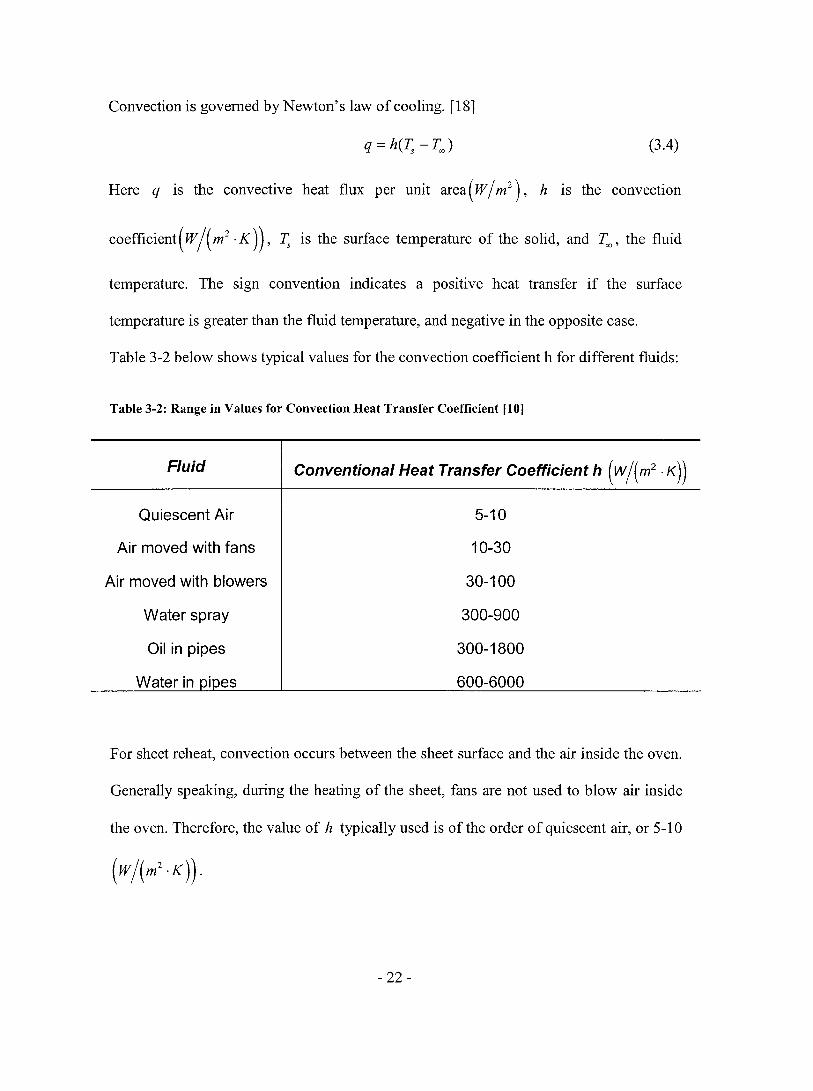
Convection is govemed by Newton's law of cooling. [18]
(3.4)
Here q is the convective heat flux per unit area ( W / m2 ), h lS the convection
coefficient ( W / ( m2 • K ) ), T, is the surface temperature of the solid, and Too ' the fluid
temperature. The sign convention indicates a positive heat transfer if the surface
temperature is greater than the fluid temperature, and negative in the opposite case.
Table 3-2 below shows typical values for the convection coefficient h for different fluids:
Table 3-2: Range in Values for Convection Heat Transfer Coefficient [10]
Fluid
Quiescent Air
Air moved with fans
Air moved with blowers
Water spray
Oil in pipes
Water in i es
Conventional Heat Transfer Coefficient h (wj{m2 .K))
5-10
10-30
30-100
300-900
300-1800
600-6000
For sheet reheat, convection occurs between the sheet surface and the air inside the oven.
Generally speaking, during the heating of the sheet, fans are not used to blow air inside
the oven. Therefore, the value of h typically used is of the order of quiescent air, or 5-10
- 22-

3.1.3 Radiation
Thennal radiation is the third mode of heat transfer. Energy is radiated from a body due
to its surface temperature along the intennediate portion of the electromagnetic spectrum.
Thennal radiation occurs between 0.1 and 100JLm, encompassing aIl ofthe visible and IR
regions, as weIl as a portion of the UV range [18]. Note that certain properties examined
in this section (emissivity, transmittivity, etc.) are wavelength-dependent. To get the total
emissivity, for instance, the wavelength dependent value for the emissivity needs to be
integrated over the entire wavelength range (from 0.1-100JLm). For the remainder ofthis
thesis, only total values will be considered.
An ideal radiator, or blackbody, emits thennal energy at the following rate, according to
the Stefan-Boltzmann law [18]:
q = crT4 b s (3.5)
Here, qb is the energy flux emitted per unit area by the blackbody( W / m2), cr is the
Stefan-Boltzmann constant ( cr = 5.669x10·8 W /( m2 • K 4
)), and ~ IS the surface
temperature ofthe blackbody.
3.1.3.1 Emissivity
A blackbody is so named because materials that obey the Stefan-Boltzmann law do not
reflect any radiation. In other words, aIl radiation that strikes the surface of the
blackbody is absorbed. However, most bodies occurring in nature obey the following
relation [15]:
- 23 -

(3.6)
If, in Equation (3.6) above, the total energy incident onto the surface of a body is 1, then
the reflectivity 11 is the fraction that is reflected, the absorptivity a is the fraction
absorbed, and the transmittivity "[ is the fraction transmitted. For most solid materials, "[
is considered to be zero, as thermal radiation is not transmitted through the body [15].
This type ofbody is called a gray body.
To define total emissivity (since emissivity alone depends on wavelength) of a body,
assume two bodies of exactly the same size, one black and one gray, are at thermal
equilibrium, meaning each is receiving exactly as much energy as it is emitting. For the
gray body, the equilibrium equation is:
(3.7)
q. is the heat flux striking the surface area, A , of the body, and a is its absorptivity. q ais 1 b
the power emitted by the gray body. For the black body, the equilibrium equation
becomes:
(3.8)
Here, qbrepresents the power emitted by the black body. The ratio of the emissive power
of the gray body to that of a black body, at the same temperature is defined as the
emissivity of the body [15]:
(3.9)
Then the total emissive power emitted by a gray body, using the Stefan-Boltzmann law,
lS:
- 24-

(3.10)
Emissivity values vary from 0 to 1, depending on the smoothness and regularity of the
body surface. In Table 3-3 below, it can be noted that a more polished surface has a lower
emissivity than an oxidized, rough surface, especially for metals.
Table 3-3: Emissivity of certain materials [18]
Material Emissivity
Polished metals 0.03-0.13
Metals, as received 0.1-0.4
Oxidized Metals 0.3-0.7
Oxides, Ceramics 0.4-0.8
Carbon, Graphites 0.75-0.9
Minerais, Glasses 0.8-0.95
Plastics 0.9-0.95
aints, Anodized finishes 0.9-0.97
The net radiative heat flux between an emitter (heating element) and a receiver (plastic
sheet) is given by the following equation [10]:
(3.11)
qrad is the net radiative heat flux per unit area, cr is the Stefan-Boltzmann constant, 1;, is
the surface temperature of the heating element, and 1'. is the surface temperature of the
sheet. Eefj is called the gray body correction factor and is defined below [10]:
- 25 -

(3.12)
Eh is the emissivity of the heating element, and Es is the emissivity of the plastic sheet.
From equation (3.12) above, it can be assumed that the emissivity of the plastic sheet is
0.95. However to find the emissivity of the ceramic heating element used in the
thermoforming oyen, sorne experimentation was needed. The section below describes the
methodology used to determine an experimental emissivity value for the heating element.
3.1.3.1.1 Heating Element Emissivity Calculations
Test setup
Using a c10sed oyen, temperature measurements (both surface and embedded) of a black
body and the heating element in question will be taken. The c10sed oyen is chosen so that
each of the bodies in question can receive an equal amount of energy; in other words,
there are no energy losses due to convection. The oyen used in the experiment is shown
in Figure 3-1.
- 26-

Figure 3-1: Closed Oven used in heating element emissivity calculations
At steady-state within the closed oyen, any body will receive as much energy as it emits.
Therefore, the portion of energy qrad emitted by the oyen and received by the body is
equivalent ta the energy emitted by that same body, whether the body is black or grey.
The radiative heat rate equation can then be used to determine the emissivity of the
heating element:
(3.13)
Here cr is the Stefan-Boltzmann constant, Eb is the emissivity of the body, ~ is the view
factor (see Section 3.1.3.2 for a description ofview factors), and 1;, is the temperature of
the body.
The "black body" in this case is a small rectangular block of polished and sanded
aluminum (87mm x 73mm x 12mm) that has been painted black with thermal paint. A
small hale has been drilled I8mm into the black in order to insert the thermocouple
which will be measuring the embedded "black body" temperature. The importance of
using the black body is to ensure an emissivity of 1, since aIl energy should be absorbed
- 27 -

by the black body.
Assuming that the radiant energy received by both the black body and the heating
element is the same, the following simplifications to equation (3.13) above can be made:
qrad (BB) = qrad (heater)
crf.BBFBBTB~ = crf.hFh~4 (3.14)
As both bodies are very close together, and are small when compared to the oyen, then
the ratio of their view factors becomes the ratio of their surface areas.
(3.15)
The emissivity of the black body is 1 by definition. AIso, cr can be eliminated from both
sides. Finally, the equation for the emissivity of the heater can be obtained:
(3.16)
So there are four factors that affect the emissivity of the heating element: the respective
surface are as of the black body and the heating element, as well as their respective
temperatures, measured in Kelvins.
The surface area of the rectangular black body was measured to be 16542 mm2. AIso, the
surface area of the heating element was estimated to be 34800mm2, assuming that the
heater was rectangular, with the following dimensions: 240mm long, 60mm wide and
1 Omm thick.
Experimental results
Tests were performed at 150°C, 250°C, 350°C, and 450°C in order to determine whether
the emissivity of the heating element depends on the ambient temperature. If so, then this
- 28 -
would have to be incorporated into the mode!.
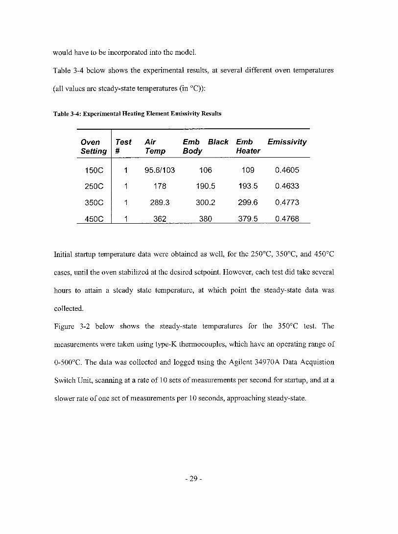
Table 3-4 below shows the experimental results, at several different oven temperatures
(all values are steady-state temperatures (in 0C)):
Table 3-4: Experimental Heating Element Emissivity Results
Oven Test Air Emb Black Emb Emissivity Setting # Temp Body Heater
150C 1 95.6/103 106 109 0.4605
250C 1 178 190.5 193.5 0.4633
350C 1 289.3 300.2 299.6 0.4773
450C 1 362 380 379.5 0.4768
Initial startup temperature data were obtained as welI, for the 250°C, 350°C, and 450°C
cases, until the oven stabilized at the desired setpoint. However, each test did take several
hours to atlain a steady state temperature, at which point the steady-state data was
collected.
Figure 3-2 below shows the steady-state temperatures for the 350°C test. The
measurements were taken using type-K thermocouples, which have an operating range of
0-500°C. The data was collected and logged using the Agilent 34970A Data Acquistion
Switch Unit, scanning at a rate of 10 sets of measurements per second for startup, and at a
slower rate of one set of measurements per 10 seconds, approaching steady-state.
- 29-

Emissivity Testing (Startup Temperatures at 350C) 302 •••• •
··,· .. •• ...... 4~ : .'t ........ ,.Jt ... ~
300 - - - - - - - - - - - - -1- -------------~~_.:_'-'~ ~::~~~._. -+-'-'~ ~~~~.-~._.~! ~ ~._,_._._~ ~~~.-'-~ ~i ~ ~ ~ ~~~ .. ~~~~~~~_.!: ------- --1 1 l , 1 1
~._~ __ ~ __ ~-~ _______ ~ ___ ~. __ ~ __ .~~._:4-' ... -~-..... --: l : : i 1
1 1 " , '" l , l , 1
------------ ... --------------+-------------- .... --------------0-------------- .. -------------l , l , , 298 1 1 l , , 1 1 l , , , 1 l , , , , 1 1 1 l , l , 1 1 1 1 l , , , , , 1
Ô : : : : : : g 296 -------------i--------------i--------------t--------------f--------------:--------------l-------------
~ : : • . - O-.en Air :::J •• _ _ Embedded Black Body 1§ :: •••• Embedded Heater Q) • • E 294 ~ ~~~ ~ ~ ~ ~ ~ ~ ~ ~ ~:~ ~ ~~ ~ ~ ~~ ~ ~~ ~ ~; ~ ~ ~~ ~ ~ ~ ~~ ~~ ~~ ~: ~ ~ ~~ ~ ~ ~~ ~~ ~ ~ ~ ~f ~ ~ ~ ~ ~ ~ ~~ ~~ ~ ~ ~ c~~ ~ ~ ~~ ~ ~ ~ ~~ ~ ~ ~ ~ ~ ~ ~ ~ ~ ~ ~ ~ ~~ ~ ~ ~
~ : i i : i , l , 1 1 1 l , 1 1 , l , 1 1 1 l , l , , l , 1 1 1 l , l ,
292 ~~~~~~~~~~~~~:~~~~~~~~~~~~~~~~~~~ ~~+~~+~~~~~~~~ ~~+ 1 l , , , t
1 l , , , l , 1 · .. · .. · .. · .. · .. · . ____ J ______________ l ______________ '- ______________ , ______________ J ____________ _ 1 1 1 l , 1 1 1 1 .. .
1000 2000 3000 4000 5000 6000 7000 Time (in sec)
Figure 3-2: Steady-State Temperature Curves at 350C Setpoint
3.1.3.2 View Factors
The final component of the radiative heat transfer equation is called the Vlew factor.
Simply put, it corresponds to the fraction of energy emitted by surface Al that is received
by surface A2 .
Figure 3-3: Radiation ray tracing between finite parallel plate elements [lOI
- 30-

The intensity of radiation emitted by a surface element dA] is constant in a hemisphere of
radius r from the surface. Any surface, dA.z for instance, collecting radiation from another
receives an amount that is proportional to its projection onto the surface area of the
hemisphere [10]. The radiative heat flux equation then becomes:
(3.17)
The view factor Fis represented by the double-integral term. cos~; are the direction
cosines, and r is the solid angle radius between elements.
The reciprocity relation for view factors was derived for black bodies, but can apply to
diffuse (meaning reflected energy is equally transferred in aU directions) gray bodies as
well. It states:
(3.18)
The reciprocity relation states that the fraction of energy leaving surface land striking
surface j ( Fi)) is proportional to the fraction of energy leaving surface j and striking
surface i (Fj;) by the ratio of their respective areas. This equation is useful for
determining one view factor from another.
Incorporating an these elements, the final net radiative heat transfer equation becomes:
(3.19)
3.2 Plastic Sheet Modeling - Energy Absorption within the Sheet
Moore [16,17] developed a comprehensive model of the plastic sheet, using the basic
heat transfer equations above. The sheet itself was discretized into several layers, each
- 31 -

defined by anode upon which boundary conditions were applied. This section explains
Moore's sheet model in more detail, with sorne improvements regarding the absorption of
energy within the plastic sheet.
3.2.1 Moore Model of Plastic Sheet
Moore divided the plastic sheet into N nodes, each a distance &' from the next. Node 1
represented the upper surface of the sheet and no de N the lower. Convention dictates that
the node be located in the centre of each isothermallayer [15].
-.. 1
• 2
• 3
• • • • N-2
• N-1
-.. N
/::,.zl2
/::,.z
/::,.z
/::,.z
/::,.z
/::"z/2
Figure 3-4: Plastic Sheet Discretization
Moore hypothesized that the primary mode of heat transfer occurring at the sheet surface
was due to radiative heat transfer, proven later by Boulet et al., [26] with sorne
- 32 -

cooling effects due to natural convection and conduction. The energy balance equation
for the surface nodes, 1 and N, is given below:
(3.20)
This equation states that the rate of change of energy for the outennost layers is equal to
the energy flow rate into the layer minus the energy flow rate out of the layer. Dividing
this equation into contributions from each heat transfer mode gives:
---- + -- T. -T. dT; 1 [ kA ] dt - pVCp qrad qconv & (\,N 2,N-\)
(3.21)
Note that, using the convention described above, the volume V in this case is equal to the
area A of the surface multiplied by &/2, as the height of this layers is haif the size of the
others.
The conduction heat transfer from nodes 1 to 2 (or N to N-I) is given by kA (~ N - T2 N-\)' &' ,
The tenns q rad and q conv are given below:
qconv = h(Too - T;,N) (3.22a)
qm' ~ œ"A, [t,( T,:",~ - 7;:")F, 1 (3.22b)
Here M denotes the number of independent heater banks in the thennofonning oven.
Within the sheet, conduction was presumed to be the sole mode of heat transfer, as the
sheet sIowly increased in temperature. The one-dimensionai conduction equation is then
used for the interior nodes of the sheet:
(3.23)
- 33 -

Using a simple approximation for the second order term, the equation becomes:
(3.24)
However, the assumption that the energy within the sheet would be solely transferred
through conduction was shown to be false. Sorne of the radiative energy striking the sheet
surface actually penetrates into the surface before being absorbed by the plastic. This was
demonstrated by Boulet et al. [26] in experimental research with thick sheets (12mm) at
CNRC-NRC IMI.
Star! ofTemperature Heating CUI\eS for 12mm Sheet at 280C 29,------,------,------,------,------,------,------,
û §. il!
28 -------------,----------
27
26
.2 25 ------------ΠQ) Cl. E Q)
t- 24
23 ------------+-------------~----
11mm
----..,-------------
." ;'1mm
9mm
, ,-.': __ : _______ ... ~ ___ i-5rnm----
: ,. ~ . ..;.
----.,.--------
21~ ____ ~ ______ ~ ____ _L ______ L_ ____ _L ______ ~ ____ ~
o 5 10 15 20 25 30 35 Time (in sec)
Figure 3-5: Start of Heating Curves for 12mm sheet at 280C
Since aU thermocouples used in this experiment indicate an increase in temperature at
- 34-

approximately the same time (8 seconds), the internaI temperatures must be affected by a
heat transfer mode other than conduction. If conduction were the sole mode of heat
transfer for these depths, then a staggered start to the heating process would be seen
above. Therefore, a secondary mode of energy transfer must be happening as weIl. This
can only be due to radiation, which means that a certain portion of the energy enters into
the sheet directly from the start of heating. Therefore the transmittivity of the plastic is
not zero. The material then must absorb sorne of this transmitted energy as it passes
through the sheet. This absorption of energy is described in detail in the section below.
3.2.2 Energy Absorption within the sheet
In a thermoforming oyen, the heating element radiates energy towards the plastic sheet
surface. The largest part of the energy is absorbed by the sheet (95% for a typical plastic -
Table 3-3) and a small portion is reflected. Of that 95%, sorne is absorbed by the sheet
itself, and sorne is transmitted through the sheet. In this case, the transmittivity 7 is Dot
zero. Therefore the energy balance equation for the interior nodes becomes [4]:
(3.25)
According to the Beer-Lambert Law [26], the transmittivity of a material depends on two
main parameters: the spectral absorption coefficient of the material, as weIl as the
material thickness. The law is stated below:
(3.26)
Note how both the transmittivity and absorptivity properties are wavelength-dependent.
- 35 -

Let A be the average absorptivity of the material across its spectrum. AlI that remains is
to discretize the continuous transmittivity function, so that the amount of energy
dissipated in each layer can be easily found.
Looking at the discretized sheet from Figure 3-4, it is noted that the exterior thicknesses
are equal to &/2, and the interior ones equal to &. When the net radiative heat flux of
intensity qrad strikes the sheet surface, a portion of qrad is absorbed inside the first zone
and another portion is transmitted through the zone. By definition, the absorbed fraction
of q rad is ~ ( z ), where z is the depth within the sheet. The calculation of ~ ( z ) is done
using the Beer-Lambert law. Then, when the thickness of the zone is&, the total
absorbed energy becomes equal to the integral sum of all energies absorbed over that
distance:
&
~(&)= fAe-AZdz o
~(&) = [1- e(-A&) ] = ~in (3.27)
Here A is the absorption coefficient with units of m -1 • With the thickness of the zone
equal to &/2, the absorbed energy becomes:
&/2
~(&~) = f Ae-Az dz o
~(&~) = [1- e(-A&h) ] = ~ex (3.28)
Assuming a radiant source located on the top of the sheet shown in Figure 3-4, the
following calculations can be made using the definitions above:
The absorbed energy in zone 1 is equal to:
- 36 -

(3.29)
The radiant energy transmitted through zone 1 is simp1y equal to the remainder:
Q = Qt1 +Qal
Qt1 =(l-~ex)Q (3.30)
The absorbed energy in zone 2 is:
Qa2 = ~inQtI
Qa2 = ~in (1- ~ex)Q (3.31)
The radiant energy transmitted through zone 2 is:
QtI = Qt2 + Qa2
Qt2 = (1- ~in )QtI = (1- ~in )(1- ~eJQ (3.32)
Similarly for zone 3, the absorbed energy becomes:
(3.33)
The transmitted energy through zone 3:
For zone n, the following equations for the absorbed and transmitted energy can be
derived:
Qan = ~in (1- ~in r-2
(1- ~ex)Q
Qtn = (1- ~in r- I (1- ~eJQ
For the bottommost zone (zone N), the equations become:
QaN = ~ex (1- ~in t-2 (1- ~ex)Q
QtN = (1- ~in t-I (1- ~ex)2 Q
(3.35)
(3.36)
The 1ast equation corresponds to the radiant energy transmitted through the entire
- 37 -

thickness of the plastic sheet. So the absorbed energy inside the plastic sheet is the
difference between the energy entering in the plastic sheet and the energy transmitted:
(3.37)
The remaining section of this chapter will serve to put together the complete model for
the heating element-plastic sheet system.
3.3 Complete Heater-Sheet State-Space Model
The state-space model of the heating element-plastic sheet system is discussed in this
section. Using the derivations above, along with parts of the Moore model, a detailed
representation of the CNRC-NRC Il\1I thermoforming machine (AAA) is obtained. It will
then be tested against experimental data. Sorne tuning of the model parameters
(conduction, convection, absorption coefficients, etc.) will be needed to correlate the
results of the simulation to the experimental data.
3.3.1 Definitions
Many state-space systems can be defined from first princip les and initial conditions. The
differential equations that describe the system can then be tumed into equations of the
following form [12]:
i = Ax+Bu
y =Cx+Du (3.38)
Here, x represents the state of the system, u represents the inputs, and y the outputs.
A , B , C, and D (often D = 0 ) are the matrices that relate each of them to the other.
The sheet is divided into 6 equal zones, each with 5 layers, making a total of 30
- 38 -

different locations at which the temperature will be calculated. Each of these is defined as
a state of the system. There are 12 sets of heating elements, each with its own PID
controller. Each of these is considered an input to the system. The outputs can be selected
as desired, by choosing the entries of matrix C . Then, the temperature at any point within
the sheet, or on the sheet surface, can be examined during the entire heating cycle.
3.3.2 State equations
The state equations for this system are derived from the energy balance equations seen
above. Let the plastic sheet be divided into M zones. For a given sheet zone i, the energy
balances at the sheet surface are similar to those seen in the Moore model, but the
absorption terms have been included:
(3.39)
Note that the temperature at node 1 for zone is given by 7;1' and the temperature at
no de 5 is given by 7;5 .
Within the large brackets, the first term represents the conduction heat transfer, the
second convection heat transfer, and the final term represents a combination of radiation
heat transfer, energy absorption and energy transmission. Energy is absorbed both from
the top and the bottom of the sheet, as the system has radiant energy sources (heating
elements) acting on both sides of the sheet. Therefore, there are both upper and lower
absorption terms. The indices correspond to the node number in each case. Here the first
- 39-

term in the large bracket represents conduction as above, but the second term represents
energy transmission and absorption only.
The energy balance equations for the interior layers also resemble the Moore equations.
But with absorption inc1uded, they become:
(3.40)
The absorption terms are described in greater detail here, for the upper and lower heat
sources respectively:
Q1jl = PlQR1j
Q1j2 = P2 (1- Pl ) QR1j
Q1j3 = P2 (1- P2 )(1- Pl )QR1j
Q1j4 = P2 (1- pJ2 (1- Pl )QR1j
Q1js = P2 (1- P2 f (1 - Pl ) QR1j
QB;S = P2 (1- P2)3 (1- Pl )QRB;
QB;4 = P2 (1-P2)2 (l-Pl)QRB;
QB;2 = P2 (1- Pl ) QRB;
QBil = PlQRB;
The total radiant energy (both top and bottom) hitting the sheet is shown below:
- 40-
(3.41)
(3.42)
(3.43)

Here, PT and PB represent the number of heating element zones on the top and bottom of
the oven respectively. Similarly, Ts and Ts are the surface temperatures of each heating Ti Bj
zone. In order to fit these equations into state-space form, sorne simplifications must be
made. The following variables can be defined:
1 a=---
pep LU
b=~ LU
CI = (n:eff~1
c2 = m:eff~1 (1- ~2)
c3 = (JEeff~2 (1- ~I )(1- ~2)
C4 = (JEeff~2 (1- ~I )(1- ~2)2
Cs = (JEeff~2 (1- ~I )(1- ~2 t Finally, the state-space matrix equations for zone i become:
·i -2a(h+b) 2ab 0 0 0 XI
·i X2 ab -2ab ab 0 0 . i x3
0 ab -2ab ab 0 ·i x4 0 0 ab -2ab ab ·i 0 0 0 2ab -2a(h + b) Xs
2ah 0 2cI 2cs 0 0
[T ] Cz C4
[Q~T 1 + 0 0 c()top a
+-- c3 c3 T (JE QRB 0 0 "'bol/am eff
C4 Cz
0 2ah 2cS 2cI
(3.44)
i XI
i x2 i x3
i x4 i
Xs
(3.45)
The superscript i denotes the sheet zone. The state variables are the temperatures at each
of the sheet layers. For instance, if the number of sheet zones M is equal to 6, each zone
having 5 layers, there is a total of 30 state variables.
- 41 -

One final simplification gives:
Q;, ~ crE<ff t F,. (Ts:, -7;;) ~ crE<ff {[ t Vs:, ] - FT, (x:)' }
Q", ~ crE <ff ~ FB, (Ts:, - 7;:) ~ crE <ff {[ ~ FB, Ts:, ] - FB, ( x; )' }
The final version of the matrix equations for zone i can then be written as follows:
2c] 2cs PT 2c]Fr 2csFB
c2 c4 IFrls: c2 Fr c4 FB l(~)'j Xi = Axi + BooToo + a j=] )
c3 Fr c3 FB c3 c3 -a PB
(x~ r c4 c2 IFB,Ts:. c4 Fr c2 FB 2cs 2c]
j=] J
2csFr 2c]FB
(3.46)
(3.47)
The problem with building a controller for this system becomes apparent when the final
term of the above equation is observed. The radiation heat transfer portion of the energy
balance depends on the temperature at the sheet surface to the 4th power, which is non-
linear. For this reason, complex robust linear controllers, like H-infinity and model
predictive control, may prove difficult to use to control the system.
3.3.3 Model Validation
In order to be able to use the model to design a controller for the system, the model must
first be validated. In other words, experiments must be performed so that the model can
be tuned to the parameters of the actual sheet-heater system. Then this tuned model can
be used to simulate the actual plant of the system.
3.3.3.1 Test setup
Testing was done in the AAA thermoforming oven at CNRC-NRC lML In order to
- 42-

properly determine the conduction and absorption properties of HDPE, a sheet thick
enough to accommodate several thermocouples was needed. For this reason, a 12mm
thick sheet was used. The dimensions of the sheet were 205mm by 230mm. The test
setup is shown in Figure 3-6 below:
heo,tlng K)(),nCl~~ sensor l therMoCo~Ple ~
::::~====~=======:: r-t -, ,---'~~--------'116
1
1
~~_~_~~IL'~' ~~~Ô~ __ ~ILI ___ ~o_~~1 heo,ting bo,nd
Figure 3-6: Test Setup for Thick Sheet Experiments
The 5 thermocouples were inserted into small holes that were drilled in the sheet at an
angle of 30 degrees. The holes were drilled in such a way that the end of each
thermocouple was precisely located on the centre plane of the sheet. Thermocouples were
placed at depths of 1, 3, 5, 9, and 11 mm. The upper and lower surface temperatures of
the sheet were measured using Raytek Non-Contact Compact Series MID IR sensors. The
simulated 12rnm sheet was divided into 5 nodes, each separated by a depth of 3 mm.
Therefore, the only nodes that correspond to physical thermocouple locations are at 3 and
- 43 -

9mm. The IR measurements taken at the sheet surfaces were difficult to correlate to the
simulation mode l, and therefore were not used in the comparisons. Aiso these IR
measurements will be used directly for control, whereas the internaI temperatures will
have to be inferred from the model results, as no thermocouples can be inserted into the
sheet during the heating cycle.
3.3.3.2 Experimental results
Three tests were performed, each with only the lower heater bank active. The upper bank
was turned off in order to minimize the sag effect on the sheet. Heating from both sides
decreases the length of the test, which can cause degradation of the sheet. For the first
test, the lower zones were held at 280°C. The second test saw a slightly higher setpoint
for the lower zones, 320°C. Finally, for the third test, the setpoint was at 420°C.
The first in each set of graphs below show the experimental temperature curves at Imm,
3mm, 9mm, and Ilmm, as measured from the lower surface of the sheet. The second
represents the tuned simulation data, in the centre zone of the sheet, at each of the 5
nodes (0, 3, 6, 9 and 12mm), also from the lower surface. The third graph is simply the
difference between the simulation and experimental data at 3mm and 9mm, or the
simulation error.
The model parameters that can be tuned are the following: upper and lower ambient air
temperatures, convection coefficient, heat capacity, density, conduction coefficient, and
absorption coefficient. The latter four are strictly material dependent, and only the
conduction coefficient k is not temperature dependent. However, to keep the model as
simple as possible, these temperature dependencies were not taken into account. These
- 44-

will be investigated as part of the larger McGill University-CNRC-NRC lMI research
program.
For the 280°C case, the results are shown in Figure 3-7, Figure 3-8, and Figure 3-9.
Experimental Temperature CUMlS at 280C for 12mm sheet 140,-----r-----,-----,------,-----r-----,----~----_,----_,
: : : : : : ' .. -.. -.. ~.-_. : : : 1mm -:---..... .!-_--l"'-p-~""1.~ ..... ,,~"'H" .... l : : _-- ... -+-::::-::~~~F~~jPH.,~~$<P~u~",;o: ~3mm : : .... ,.....:::4.':.T"·,.-;q.<~~~~r;·~ : _.J...-.-.~ .. - ........... -_ ... : :;"":~$l"'-fl": ... _.,.. .... __ .;-.....: : ~
120 ----- ___ ~--------/l';."------;;.;;;_~------:-----------:--------- _" ___________ c __________ ~--9rnm--: ,'. ... : .. .,.,,:, '- ::
: ,; . .t." "-: l: /: : 11r!nm : N.' , :
100 1_- ----1// --+---------i-----------i-----------i---------+- -----+--------+----lI .. ': : :::
1-:1 ' , ,~ :
!/., : : -----f!- -~-------- --,------- ---j----- -----:---------- -- ---------:-----------f----------,----------
II: : : : : f : : : : 1: : ::
1: : "
0-c: '=-~ => 80 "§
'" c-E
'" 1-
60 t _____ • ___________ ( _______ : __________ -:- __________ : _____ ----r------i--------, , , ,
40 --------------------:-----------j-----------'-----------f-----------:-------------------- -,------" " " 1 1
" " " " , , , ,
20L-----l-----~----~----~-----L----~----~----~----~
a 500 1000 1500 2000 2500 3000 3500 4000 4500 lime (in sec)
Figure 3-7: 280C Experimental Temperature Curves
- 45 -

E !" ::J
~ (1) "'-E (1) f-
Simulated Model Temperature CUf\eS at 280C for 12mm Sheet 15O;-----,------,-----,------r-----,------,-----,------,-----'1------,
i Bottori, Surfac6 1 l , 1
100
50
: : ,,,..,. .. _.~ .. -,,,,.·-i·.,..·_·-~-,,-~-*i-· .... ·-~+·""'·~ 3mm : .... · .... : .. _---+----t----"'!'----"!'----:---~ /'~:;:~;~f.::::::::r-:::::::~::::::.:-~:::.::::F::::::·li-:·::·~: 6mm
: l~:" : : : : : : " • .Ji: : : : :: : --- ----~P#:--L-------l---------j--------L---------l--------j--------- ---------)---------
.l/: ' : i : i i i i9mm
/" : i i i : : 1 :
.. ! ': : : : : ' : Top Surface: ni: ': ' ::: : r. :: : : : : il :: :: : i" : :: : ii! : :: '~/: , :: 111' , " i!;'-----~ ----- ----~-- -------~ ---------i ---------~---- --- --r ---- -----r -- -------~- --------+ --------
fi, ':: i ' l , 1 ,,: : : ' : .. 1 '" ~I : : il : :
OL-____ ~ ____ _L ____ ~ ______ L_ ____ ~ ____ -L ____ ~ ______ L_ ____ ~ ____ ~
o 500 1000 1500 2000 2500 Time (sec)
3000 3500 4000 4500
Figure 3-8: 280C Simulation Model Temperature Curves
Simulation Error (vs. Experimental Data) at 280C for 12mm Sheet
5000
3r------,------,------,------,-------,-----~------,_----_,------,
, 1 l , , 1 1 1 -------,-----------r----------T-----------,-----------T----------,--- -------r----------,-----, "'" , " l , , , " l , ,
, "'" , '" , 1 l ,
, '" 1 1 l , , 1 -- ----,-----------r-----------,------------,-----------.----------.,-- --------r---, , , , , , , , , , , , , , , , , , , , , , 1 , , , , 1 , , , , t , , t , 1
1 l , , F , , , -,------------r-----------r-----------,-----------.-----------,-----------r-----------,--o -.-----l , , , , , , 1 , , , , , ,
, , , , j
1: •• ~\.j ••• ···· •• f··········I~E~"t9m~ ••.•••.. i.7( •• 1 .••••••••.
'\ : : : ,/ :
:·········:~I··········i··········I········· Time (sec)
Figure 3-9: 280C Simulation Error (vs. Experimental Data)
- 46-

For this test, the model parameters were tuned such that the resulting temperature error
curves remain within 6°C of their corresponding experimental data. The parameter values
are listed in Table 3-5 below.Figure 3-10, Figure 3-11, and Figure 3-12 show the curves
for the 320°C tests:
Experimental Temperature CUMlS at 320C for 12mm sheet 160~------~-------.--------,--------.--------== __ -----,
: ...... ----, ' .... .,. : 1mm ,,- .... .,r :
, ~.,. 1 1
140 ---------- --'- _________ )~< _______ ;,J~,~::··~~~:·~~::-1~-~~:~3~-~--1 ,.;.,;""'-: ,~""..1~-;{f'c: : l '...' ,yJ»'~" ~ 1 1 : """"~.",.",, ,..~"~~~,, .. ,.ii~~t ~ ...... _.-.-...... ~ ....... 9mm
120 --------------;--;...;;;~-~;~j:::.:: ... :~-.-~--.-~.~:~:- :----------------l----------------:, ~"'~ ",.-': : if" " , ,
// / : 11rtJm Ü 1.-\/ : : : ' §. 100 ----/:'-j- --------------j----------------~-----------------:-------------------
!':' /: /,: : .g ,t· :: : ~ li 1 :
0. 80 _____ ./~.- ______ c ________________ ; ________________ L __ _ ~ pi: l
,: : ,: , :
60': : , , : --1;' ----------;---- -----------~----------------~------- --~--------------- -,------------I~ : ' , : t;
, , _____ 1_ _ _ _ _ _ _ _ _ _ _ _ _ __ ~ __________________________________ : _________________ , _______________ _
, , , , , , , , , , , ,
20L--------L------~--------~------~--------~------~ o 500 1000 1500 2000 2500 3000
lime (in sec)
Figure 3-10: 320C Experimental Temperature Curves
- 47-

Simulated Model Temperature CUMS at 320C for 12mm Sheet 160r----------,---------,----------.----------.----------,---------~
: / Bo~om Surface 3mm
f : : ",L _" ...... _~_ .. -i,,_./ 140 ---------------t------------- :---------~:.:;;.;;~<--, .. ,..,!~-~;::.:;:,;;:,;~~~.:.;::::.::.::.:-6rÏÎm--
: : .". ........ .".. ~ ....... ------, : : ;,,~'" ",.--.",.,--:~ ........ -' .......... r ... -.-.-.-.:._··\
120 ----------- --i---~;. .. :2~;:~~:::7:·::j::::~·:::::::::·r-·-·:-·-·-·-·-·-~~~·):r::-·-·---- -----: ,,:"''iJ'' : i i i 9mm
f '"' ···· ... tY··· ··'·Trp~<>fa~1 ! 80 }<~/-;-------------~------------- : ----~ --------------:------
.' ! il : : :' ! ti':, : • l ',,' ,
60 f- ;-/t-------;- ---- ------- ---;----- ------ -"-----------~--------------:---- ----ii l : :
HI i i 40 }jL ________ -f---- -------i --,---------------:-------- : ---------------
Il' : : il : : il : : ~ :
20L----------k--------~----------~---------L----------L---------~
o 500 1000 1500 2000 2500 3000 TIme (sec)
Figure 3-11: 320C Simulated Model Temperature Curves
Simulation Error (vs. Experimental Data) at 320C for 12mm sheet 6,---------,---------,---------,----------,---------r---------,
4
-4
-6
, , f , ___________ .1 ________________ -.1 ________________ ..) _________________ , _______________ _
l , 1 , , , , , , , , , , , , : '~t.:
-----~----------------~---------- -----f---\---------------" l ,.#
.. 1 : '. \
\ ________________ - -1-------
.~
, Errorat9mm ,; i "-
'7+·······1/··1········ -+-------\---j--- --I----
: Îi ~'. ' , l : ,
-------t-------------\,-i---------------i---, .' ,
~ ,
;\ '. ---'-------------- -p\--- --------',- ---/----- ----:-- --:-------,.\. '.J l ,
500
:" V -------:- Error at 3mm : ,-,", : : " , " ,
1000 1500 TIme (sec)
2000 2500
Figure 3-12: 320C Simulation Error (vs. Experimental Data)
- 48 -
3000
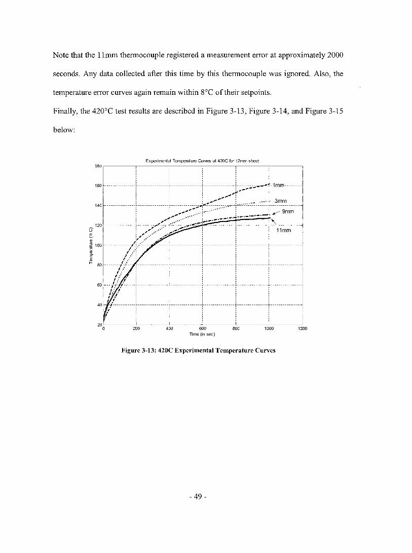
Note that the 11mm thennocouple registered a measurement error at approximately 2000
seconds. Any data collected after this time by this thennocouple was ignored. Also, the
temperature error curves again remain within 8°C of their setpoints.
Finally, the 420°C test results are described in Figure 3-13, Figure 3-14, and Figure 3-15
below:
Experimental Temperature CUM'lS al 420C lbr 12mm sheet 180,-------,--------,--------.--------,--------,--------,
---------,----------- ----~--- --- _~""':' 1mm----.. --i ,4I'r'-'~ : : ".,..",..~"'! _~H~"~"'!' 3mm
140 --- -- ---- -~~.:;-~-----;,,-;~-~,,-..-'-"-'~-"-~y.!'_~!-~~~-------+--------
1 1 .".-.,.". ~,,~+~,,~~"~"~: : / 9mm
160 ----------- ---,-----------
, ;,"-' ",,,,,,,,,,.~~~~! _ .... - .. f//II.~ .... -.-.-."""""",. 1 : ,;" :~t""''''' .-,:--·--:--.. -----------~-----------------i-\-------------0 120 1---- :------;;;;"-,~;,.:----:,;;.;. .... ' .... - : , , 11 mm
c'! ;' 4 ..... ~... ...~,..... ! : : ~ ~ ;,.1 ~",/,,,, .. .;..~"-: ! '-! " ~ , 1 .a 100 --------------,.-t:'----- ------+---------------:-----------------:-----------------:----------------
~ 1 /.": : ':
El":' : : : ~ // ' ::
80 -------t-,'--- --,- ------------ -,-----------------:-----------------:----------------1 .. : :
,'/ : : 1","" 'J'. 1 l ,
60 ---li 'I-----;------;---------------~-------I~' 1 :
1.' ,. : 1 • ' l ( : j----------;-------
:.' :
200 400 600 TIme (in sec)
800 1000
Figure 3-13: 420C Experimental Temperature Curves
- 49-
1200

Simulaled Model Temperature CUMS at 420C for 12mm Sheet 160,---------~--------,_--------,,----------r, ---------r---------,
, ,
~: Botlom ~urface , ' , 3mm
" ""'--140 -- ____________ 1-- _______________ 1___________ : - -.-.:..-.-_-.. ---.. -~.,,~'I.'""'~:_~--- -- -- -----, 6""'~-~~ ". ... ,....,-.,. .. --- : ~ : .. ;"0> "*' ....... r,.._.-· ..... :: .. ".~ .. _ .. , ........ ··r 6mm , ...... '..., -_ .. -'-':"'-''''-'-'A
··;>7~;"'r.'f·············T·······l··· ........ . 120
~ '00 VPi";L+j9mm ;:< .,;': l ' , : T~p Surface ~ .... :, : : :
~ 80 --- ----.... /I------------)-----------)--------------~-- -----------,---------f-- ./// i : : i
:' .1.11 : : : : "." ,,# ~' 1 : : : 60 :-/iF------:---------------+------------~---- ----------------
! ~ Il : : : !il : ' • J/!: :
40 -.~"f_------i------------;------{JI ' , ii l : ' ,1 ~I "
200 400
- -- ------------:----- ---- ---
600 lime (sec)
800 1000
Figure 3-14: 420C Simulated Model Temperature Curves
Simulation Errar (vs. Experimental Data) at 420C for 12mm sheet
1200
4.---------,----------,----------,----------,---------,,---------,
: '1 " .. """"\,\ ............... ,:----------------', ............... 'lA ....... . 2 : l :
--------------:-~~-------------:----------------1------ ---------T;l--------T---------------~ l '. 1
\ ,;:; ----T-- -,- {--- ------------l------------~}--i-----------------i----------------
': /: Error at 3mnjl / : ~.: : l :
, "'.: : / ,
~ 1 -
------- ---- f --- --- -~~ -------:- ---- ------ -----~- ------!-------~------
" , .,/ :" : : ...' : t
-1 ---- ---------~----------\---;----------------J--l : \ i :!
, , ..,-----------------,----------------, ,
\i / ~, " :
-2
~L---------~--------~----------~---------L--------~----------~ o 200 400 600
lime (sec) 800 1000
Figure 3-15: 420C Simulation Error (vs. Experimental Data)
- 50-
1200

For this last test, the error seems to be the closest to the setpoint, as the margin is only
approximately 3°C.
A closer look at Table 3-5 reveals the tuned simulation parameters for each case:
Table 3-5: Tuned Simulation Parameters for 280C, 320C and 420C tests
Parameter 280C 320C 420C
Air Temp Bottom ( C) 145C 155C 155C
Air Temp Top (C) 115C 120C 120C
k (Wj(m.K)) 38.4 38.4 38.4
h (W / ( m2 . K) ) 30 30 20
p (kg/m 3) 850 850 550
C (Jj(kg.K)) p 1700 1700 1000
A (m-1) 30 30 30
% error at 3mm 0.33% 0.35% 2.28%
% error at 9mm 0.22% -0.77% -0.94%
The percent error formula used is glVen below, where Experimental is the final
experimental temperature and Simulated is the final temperature from the simulation:
Percent error = Experimental - Simulated xl 00% Experimental
(3.48)
It quickly becomes clear that the 420°C test parameters are not logical. To make the
simulated temperatures resemble the experimental ones, certain parameters, namely
- 51 -

density (p) and heat capacity (Cp) were chosen well outside of their acceptable range
for HDPE. AIso, the ambient air temperatures cannot be the same for the 320°C test and
the 420°C test. Simple measurements have been performed indicating that the air
temperature should be at least 175°C above the sheet and close to 200°C below it for a
heater setpoint of 420°C.
For the other two cases, the material parameters obtained via simulation are close to the
nominal values for HDPE. Similarly, the physical parameters of the system approach
those measured during other testing (ambient air temperatures). The only parameter not
within nominal range is the convection coefficient, h . Because of the large openings at
either end of the oven, there may be unseen air currents causing major conduction effects
at the sheet surfaces, such that the upper sheet surface temperature is higher than the
lower sheet surface temperature, contrary to a more typical oven, where the lower surface
is hotter.
Other potential reasons for error are enunciated more clearly below:
3.3.3.3 Reasons for error
The simulation model remains a work in progress, for several reasons. Each of the
temperature dependent parameters must be adjusted as the temperature of the sheet
increases. So, for instance, the constant heat capacity can be replaced with a temperature
dependent version, thereby improving the response of the model. For instance, increasing
the heat capacity will have an effect on the transient response of the sheet model. This
increase will create a larger thermal inertia. Therefore, it will take more energy to heat
the same amount of plastic, which essentially means a slowing down of the transient
- 52 -

response of the sheet model. A similar temperature-dependent function can be
implemented for the density as well. These functions are being investigated by other
students and researchers at McGill and CNRC-NRC lMI.
There are also a couple of important points regarding the heating elements themselves.
The model views each oyen zone as a large heater block, of size 30cm by 30cm
approximate1y. However, the actua1 oyen is composed of 3 heating e1ements each of size
6cm by 25cm, with a small4cm gap between each heater (see Chapter 4 - Figure 4-4 for
the oyen dimensions). These small gaps do not represent much surface area by
themse1ves, but when added up, they total 40% of the oyen surface. Therefore, the mode1
overestimates the amount of actua1 heating surface area when the oyen is heating the
sheet. However, this prob1em may be counterba1anced by another physica1 phenomenon.
The heating e1ement does not uniform1y heat to the temperature setpoint of the PID.
Figure 3-16 be10w shows an actua1 representation of the surface temperature of a heating
e1ement at a setpoint of300C, taken with the AGEMA Infrared camera.
- 53 -

Figure 3-16: IR temperature measurement of Heating Element Surface (setpoint 300C)
The temperatures along the line LlO 1, as well as a histogram showing the temperature
distribution over the whole line are given below:
::)45 :305 264 224 :184 144 1..0,4
64 *' 24
' .... ....
l
Figure 3-17: Ll01 data li ne from IR Camera picture above (setpoint 300C)
- 54 -

345 3:13 281 240 2:16 184 :l52 120
98 5&
0.,0 &9.9 :1.3_5
6_4 3_2 0_6 0 ... 6 0",,6 2",,6 2.6· 0.0.
Figure 3-18: Histogram showing temperature distribution along line LIOI
The embedded thermocouple measuring the temperature that is compared to the PID
setpoint appears to be in a "co Id" spot when compared to the rest of the surface area of
the heating element. This shows that the model is underestimating the surface
temperature of the whole heating element by taking the lower setpoint value instead of
the actual value. These two effects combined need to be studied in greater detail so that
the simulation model developed in this chapter can be completed.
Finally, the model tuning performed above is done with one large assumption: that the
sheet exhibits only one-dimensional conduction heat transfer (i.e. through the depth of
the sheet). It assumes that the sheet is thin enough that each sheet zone does not lose (or
gain) any conduction energy from its adjacent zones. This assumption may not hold true
for these sample tests, as the sheet used was 12mm thick. This is another area where the
model can be improved.
- 55 -

Chapter 4 Real-time control of AAA Thermoforming oven
Real-time control of any process is a complicated and difficult task to accomplish. Often,
for industrial processes like thermoforming, any control effort is done in open-Ioop. This
means the machine operator checks the final result (i.e., a thermoformed sheet), and
adjusts the settings on the machine if the results are not satisfactory. The operator will
then "tweak" the machine settings until he/she gets a part that is deemed acceptable. The
settings are then left alone until shutdown or until machine drift has caused part eITors,
whereupon the entire "tweaking" pro cess will have to be repeated. However, using the
OPAL-RT RT-LAB real-time operating software, real-time control becomes much easier
to implement. Infrared sensors are placed in positions such that specific sheet surface
temperatures are measured with 0.1°C accuracy. The sheet temperatures can then be
controlled as desired during the heating cycle.
First, an overview of the AAA thermoforming machine at CNRC-NRC lMI will be
given. The existing control structure of the system will be examined, a PlO feedback
control loop connected to Solid-State Relays. These relays act as switches, allowing
CUITent to flow through the heating elements when the PlO output is high, and blocking
the CUITent when it is low. AIso, the actuators of the system (the heating elements
themselves) will be studied, more specifically their heating and cooling rates (which are
not the same). Then the IR sensors will be investigated as wel1: a brief explanation of
how they work, how they are calibrated, and where they are located within the AAA
oyen. Finally, a description of the OPAL-RT RT-LAB hardware and software used to
develop and operate the real-time model and controller will be shown as weIl.
- 56-

The next section of this chapter will focus on the control algorithm proposed and
implemented for the AAA thermoforming machine. The multilayer algorithm will be
broken down into its inner and outer loops. The inner loop will focus on the replacing of
the hardware PID control with a software version within the RT-LAB model. The outer
loop will focus first on developing the steady-state relationship between the heating
elements and the temperatures measured by the IR sensors in different locations. Using
this steady-state gain matrix, a basic PI controller is then implemented for each of the IR
sensors for both step and ramp inputs.
4.1 AAA Machine Overview
First, the AAA thermoforming oven used at CNRC-NRC lMI will be examined. The
zones ofheating elements, the PID blocks used to monitor and control the temperature of
each zone, and the oven layout will all be discussed. Then, the hardware added to the
AAA machine for the purposes of real-time process control will be described. The
infrared sensors and the OPAL-RT RT-LAB operating software will be discussed one at
a time.
- 57 -

4.1.1 System Actuators and Layout
The AAA therrnoforrning machine at CNRC-NRC Th11 is shown in Figure 4-1 below. By
therrnoforrning machine standards, it is small, used to forrn small sheets of 69 cm x 99
cm maximum. Note that the sheet enters into the oyen between the trays of heating
elements, which are situated above and below the sheet entry plane.
Figure 4-1: AAA Thermoforming machine (front view)
Inside the oyen, the heating elements are arranged in the following manner: 36 heating
elements are split equally between top and bottom, divided in such a way that there are
12 heating zones. Each zone contains 3 heating elements connected in parallel, one of
which is shown in Figure 4-2. Each Tempco-made heating element supplies up to 650W
of 3-phase power. The basic ceramic infrared heater design consists of a high
temperature nickel-chromium alloy resistance coil evenly distributed and embedded into
the ceramic during the casting process. The coil is located as close as possible to the
element surface in order to deliver maximum efficiency. The range of infrared
wavelengths is from 2-1 OJlm [27].
- 58 -

Figure 4-2: Tempco 650W Heating element
The heating elements are laid out in a similar manner, top and bottom. A view of the
lower tray can be seen in Figure 4-3 below:
Figure 4-3: Lower Heating tray
The exact dimensions of the heating tray are given in Figure 4-4.
- 59 -

1· 78 cm ~I
~ t 4.1 cm
57.1 cm ~ 26.5 cm 4.1 cm
1
6.1 cm
1· ~I 4r- 1 24.6 cm 2.1 cm
Figure 4-4: Top view of AAA Oven
4.1.2 Existing Control Structure
The central heating element in each zone has an embedded thermocouple. This
thermocouple sends a signal to a PID controller, which maintains all three of the heating
elements (including the two without thermocouples) in that zone at the given setpoint
temperature. Figure 4-5 below shows the LED displays of the PID controllers.
- 60-
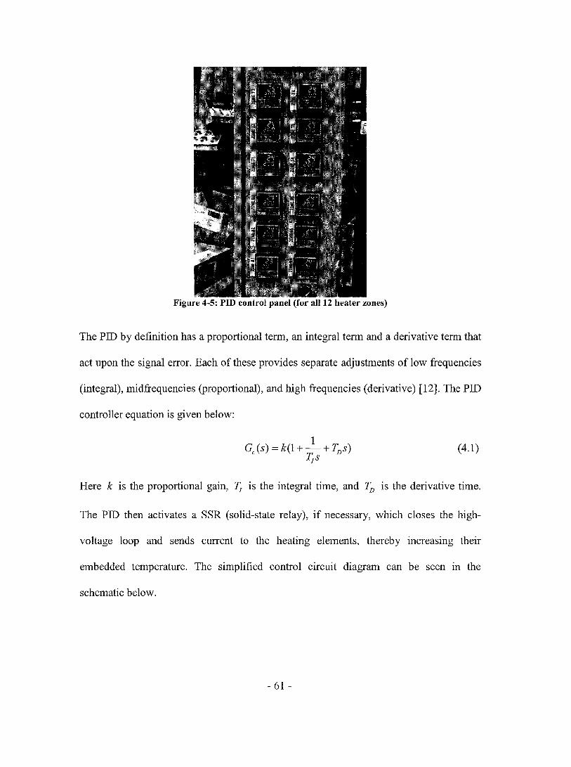
Figure 4-5: PID control panel (for ail 12 heater zones)
The PID by definition has a proportional tenn, an integral tenn and a derivative tenn that
act upon the signal error. Each of these provides separate adjustments of low frequencies
(integral), midfrequencies (proportional), and high frequencies (derivative) [12]. The PID
controller equation is given below:
(4.1)
Here k is the proportional gain, ~ is the integral time, and TD is the derivative time.
The PID then activates a SSR (solid-state relay), if necessary, which closes the high-
voltage loop and sends current to the heating elements, thereby increasing their
embedded temperature. The simplified control circuit diagram can be seen in the
schematic below.
- 61 -

,/
12VDC SSR 208VAC /'
PID Heating Element
11\
Thennocouple data
Figure 4-6: PID Control Loop
The PID was set to a 3 second dut y cycle. When the pulsed output of the PID was high,
or 12V, the SSR allowed 60Hz AC CUITent to pass to the heating element, increasing its
temperature. When the pulsed output was low, the SSR remained open, preventing the
passage of CUITent to the heating element. The magnitude of the CUITent passing through
the heating elements was approximately 8 Amperes. This magnitude did not depend on
the length of dut y cycle.
4.1.2.1 Modeling the actuators
After developing the sheet model in the previous chapter, the next step was to develop a
relationship between the input power and the heating element temperatures. This
relationship would pro vide the final piece to the global transfer function relating the input
power to the sheet surface temperature.
- 62-

The heating element transfer function was determined by open-loop testing. The PID was
placed in manual mode, and the input was changed from a temperature setpoint to a
percentage of dut y cycle. The magnitude of the step input corresponding to the length of
the dut y cycle can be determined from the following relation:
mag ( Step ) = mag (pulse) * duty 100
(4.2)
Given that the pulsed current magnitude was ~8A, the magnitude of the step was simply
calculated according to the equation above. From there it is easy to transform the step
input into an input power, simply by multiplying the step current magnitude by the input
voltage of 208V AC. Zones B2, B5, T2 and T5 were tested in manual mode, for several
different dut y cycles. The objective of these tests was to determine the reaction of the
heating element to differences in input power, at different locations (interior and surface).
4.1.2.1.1 Test setup
Two measurements were taken, one from the embedded thermocouple located inside the
heating element (the same one the PID used as input), and the other from a Raytek
Thermalert ™ SX Infrared sens or, capable of measuring temperature without contacting
the sheet. Using a smooth, polished mirror (with no losses due to reflectivity as measured
by another Raytek instrument - the Raytek MX2 portable non-contact IR thermometer),
the Raytek Thermalert ™ sensor was pointed directly at the centre of the heating element
in order to measure its surface temperature. The data was collected using the OPAL-RT
real-time system (see section 4.1.4).
- 63 -

4.1.2.1.2 Experimental results
Figure 4-7 shows the evolution of the embedded and surface temperatures for zone B2
with a 10% dut y cycle.
E ~ ::::
T§
'" c. E '" f-
Embedded and Surface Temperature Measurements for Zone B2 at 10% Dut y Cycle
, , 100 ------- ____ c ________ --- - -- --------"-- ---- ------~------ ---
80 ~ - -- - -- -- - -r - - - - - -- - - - - --
60
o~----~----~----~----~------~----~----~----~ o 200 400 600 800
1ime (sec) 1000 1200 1400 1600
Figure 4-7: B2 Embedded Thermocouple Temperature -10% Dut Y Cycle
Each curve displays the characteristics of a first-order transfer function. Any first order
system can be described completely using two parameters [12]: the steady-state gainK,
and the time constant T. The equation is shown below, in relation to this system:
Temperature K
Duty Cycle TS + 1 (4.3)
- 64-

Table 4-1lists the parameters for B2 for several different dut y cycles.
Table 4-1: B2 parameters for sever al dut Y cycles
Surface Embedded
Step 't K 't K
0-10% 415.43 8.75 498.68 8.58
0-20% 380.53 7.40 450.91 7.36
0-40% 297.79 5.84 361.76 5.9
0-60% 277.09 5.02 336.68 5.2
0-100% 244.04 3.93 293.5 4.17
Note that the time constants in each case were very long, over 400 seconds in sorne cases.
This is a known property of ceramic heating elements, and there are other types that react
more quickly (quartz, halogen) [8]. It was beyond the scope of this project to integrate
different heating elements than those that were already installed in the AAA machine.
However, it is to be noted that the heating element would never be operated in open-loop
conditions for it would take far too long to heat a sheet to the forming temperature.
Therefore, it makes more sense to look at the final entry of the table, where the dut y cycle
is 100%. Essentially, this means that the CUITent is always passing through the element,
which mimics the initial heating much more closely. Also, the steady-state gain values
for each case were not the same, as the embedded thermocouple is not the same distance
from the wire inside the ceramic as the surface measurement.
It is apparent in all cases that the steady-state gain K and time constant 7 depend on the
- 65 -
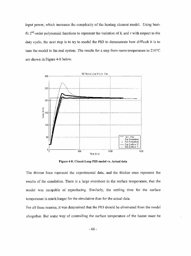
input power, which increases the complexity of the heating element model. Using best-
fit 2nd -arder polynomial functions ta represent the variation of K and 7 with respect ta the
dut y cycle, the next step is ta try ta model the PID ta demonstrate how difficult it is ta
tune the model ta the real system. The results for a step from room temperature ta 2100 e
are shawn in Figure 4-8 below.
82 Clased Laap Sim vs. Exp 300 r-------------------------------:--------------------------------:--------------------------------;
, , , , , , , , , , , , , , , r ' , , \: : : \: : :
250 --------I-----\.:----------r--------------------------------r--------------------------------j 1 -.. "- ; ; ;
1 '''' "-- : : : '-.' : : 200 ----of rl-----------------i--------------------------------i--------------------------------]
i 1ffih--l
e 100 __ ~ __________________________ • ________________________________ • ________________________________ ! , i i i
, , 50 - -----------------------------;--------------------------------;-------- - Input Step
: : - Exp Embedded : :. Sim Embedded : : - Exp Surface IR : :. Sim Surface IR
oL-------------~-------------L--~========~ o 500 1000 1500 Time (in s)
Figure 4-8: Closed-Loop PID model vs. Actual data
The thinner lines represent the experimental data, and the thicker ones represent the
results of the simulation. There is a large overshoot in the surface temperature, that the
model was incapable of reproducing. Similarly, the settling time for the surface
temperature is much longer for the simulation than for the actual data.
For all these reasons, it was determined that the PID should be eliminated from the model
altogether. But sorne way of controlling the surface temperature of the heater must be
- 66-
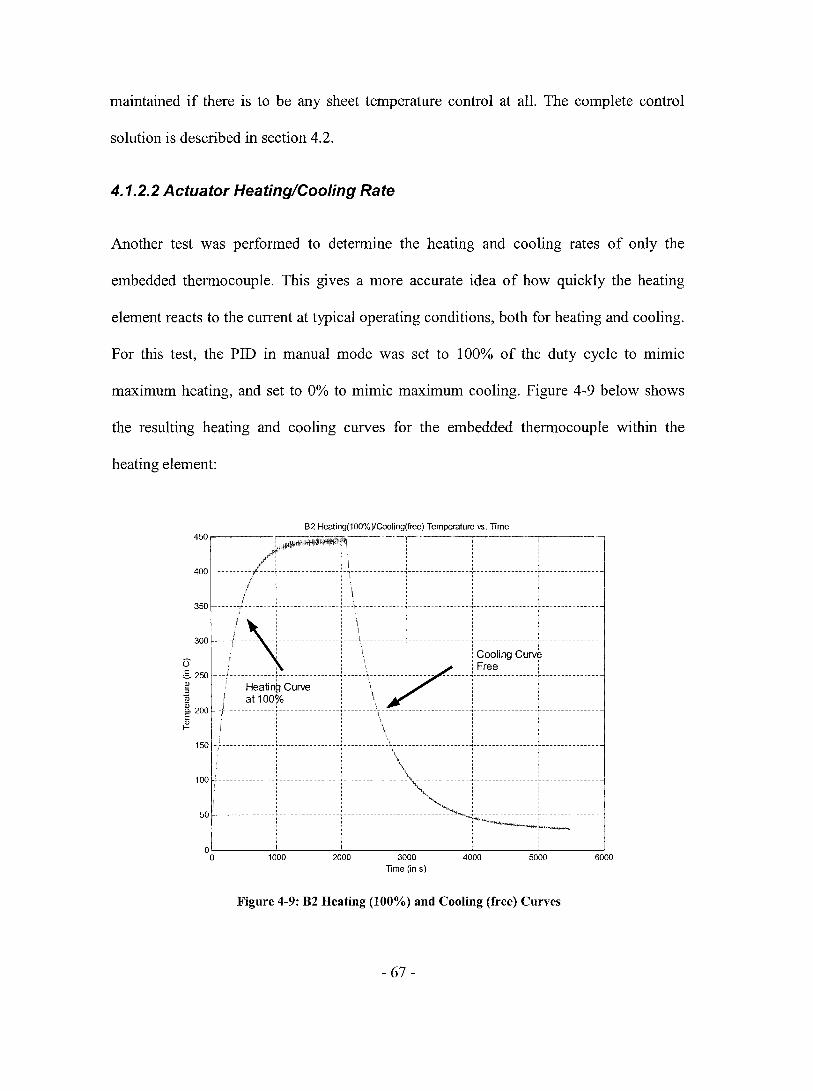
maintained if there is to be any sheet temperature control at aIl. The complete control
solution is described in section 4.2.
4.1.2.2 Actuator Heating/Cooling Rate
Another test was performed to determine the heating and cooling rates of only the
embedded thermocouple. This gives a more accurate idea of how quickly the heating
element reacts to the CUITent at typical operating conditions, both for heating and cooling.
For this test, the PID in manual mode was set to 100% of the dut y cycle to mimic
maximum heating, and set to 0% to mimic maximum cooling. Figure 4-9 below shows
the resulting heating and cooling curves for the embedded thermocouple within the
heating element:
82 Heating(100%)lCooling(free) Temperature vs. Time 450~----~r-~~~~----~'-~-----r-------r------~
400 ---------/j~~~~~=::T~----------- -~----------------~-----------------~--------------;f : ~ : ' : ! 1 : t " ; , "
: •• IqIITIT i'~J:';i;F~~i\7i~::'9C"1 ......... . ! 200 -;-------------1----------------:--------\-----+---------------+----------------~---------------
\ : 1 ~ -- - - - -- -\ --- ... - - - - - - - - - - - - - - - - .... -- -- - - - - -- - - - - -->--- ---, ' ,
\ : ' , \ l ,
150 ; !
100 .' ---- - - - - - - -- -- - ~ - - -- - - - - - - - - -- - - ~ - - - - -- -- - - --- - -~~~ - - - - - - - - - - -- - -~-- -- - - - - - -- - - -- --~ -- -- -- - - - - - - - --
! i i ~~',- i : : : : ~: ,
---------------r----------------i----------------i----------'i~~:.::~l=-------
1000
, l , ,
, "
2000 3000 Time (in s)
, ,
4000 5000
Figure 4-9: B2 Heating (100%) and Cooling (Cree) Curves
- 67-
6000

These curves are broken down further in the following table.
Table 4-2: Heating and Cooling Rates for zone B2
HEATING (100%) COOLING (Free)
Temperature CC) Heating Rate (OC/s) Temperature (oC) Cooling Rate CC/s)
27.9 1.36 445 0.96
50 1.17 400 0.67
100 0.95 350 0.55
150 0.82 300 0.44
200 0.71 250 0.35
250 0.55 200 0.25
300 0.40 150 0.16
350 0.23 100 0.06
400 NIA 50 NIA
The heating rates are greater than the cooling rates as expected. Cooling is done by free
convection, which is a natural process, and therefore much slower than the heating, which
is an active process. This phenomenon will have important effects on the controller
designs.
4.1.3 Infrared Sensors
In order to control the plastic sheet surface temperature, a non-contact method of
measuring the surface temperature must be used. If a contact method of measuring
- 68 -

temperature, like a thermocouple, were used, there could be sheet degradation at the point
of contact due to conduction. Infrared sensors are also capable of measuring higher
temperatures than contact thermocouples, at a faster rate as weIl.
The infrared thermometer can be compared to a human eye. The lens of the eye can be
seen as the optics through which the radiation from the object reaches the retina, or
detector, through the atmosphere [29]. Every object radiates infrared energy along a
given wavelength due to its temperature. The wavelength-dependent emissivity affects
the amount of energy seen by the IR detector, as discussed in the previous chapter.
Therefore, an emissivity value needs to be input into the IR sensor before accurate
measurements can be taken. In this case, the IR sensors will be evaluating the surface
temperatures of a plastic sheet. The emissivity of plastic is given as approximately 0.95
(see Table 3-3).
The Raytek Thermalert® MIC ™ Miniature Infrared Sensors must be operated within a
certain ambient temperature range. If they are used outside of this range (25-85°C)
without sorne form of cooling, they may become damaged and their measurement
precision may suffer. Observing Figure 4-10 below, the sm aIl cylindrical shaped sensor
can be seen at one end, and the square electronics housing at the other. The two pieces
are connected by an insulating tube, which protects the sensor from overheating. Cool air
is pumped into the tube to maintain the operating temperature of the sensors within the
desired range.
- 69-

4.1.3.1 Distance ta Spot Ratio
The optical detector receives the focused infrared energy of a circular measurement spot
on the object whose temperature is being measured. The optical resolution of the sens or
is defined as the ratio of the distance D of the object to the sensor with respect to the size
S of the optical spot [27]. Figure 4-11 gives an idea of two different D : S ratios:
~ ::::::=----____ --t~D:S ~lO:l
40mm T D:S =2:1
200mm
Figure 4-11: Examples of different D : S ratios
- 70-

The Raytek Thennalert® MIC™ Miniature Infrared Sensors used in the AAA
thennofonning oven at CNRC-NRC IMI have aD: S ratio of 10. This means that since
they are aU approximately placed 15-18cm away from the plastic sheet, each sensor
measures a cireular area on the sheet surface with diameter 1.5-1.8em.
4.1.3.2/R Sens or Locations
If each IR sensor measures an area of 1.76-2.54em2 (from above section), then it would
require more than 350 sensors to measure one side of a 30cm by 30cm sheet. Obviously,
this is not practical. Therefore, the foUowing sensor arrangement was chosen. In Figure
4-12 below, the star shapes represent the locations of the IR sensors with respect to the
heating elements. There are 7 IR sensors per tray, and 14 in aU.
,. 78 cm .,
\<';/,,;11-,---,--,-" ~-,------ill)'··· ,........ . 1 ~ IRT6,1~~6 ~ '. ~ IRT5. IR85
IL.' --,--"_2_" O-,-ne_T_' 1_.S'--l.1.:....· .• , •. _ .• ·'--l.·-J:I ['.' . ,'. ZOQe T3;f33 . Ii
4,1 cm
,----1 ~-----,iil '-------'r-~ ,-----l _-----'1 ~ 26.5 cm IRT7.IR8~_. __ 2_6_,7_cm ___ .+ IRT1.IR81 +IRT4.IR84 4,1 cm
57.1 cm L--l ---,--~'il ,---l ---,------,II 1 T 1 Zone T4,84 .' "",:1" Zone T5,85 Il'. : .".Zone T6,86 ,
IRT2 IR82 ~.--______ -,~IRT3 IR83 ! ----'.--1'----_---'" l ,---1 _-----"-6,1 cm
,. ., ~~ T 24.6 cm 2.1 cm
Figure 4-12: Top view of AAA oven with IR sensors
- 71 -

For the upper heater bank, the centre IR sensor is labeled Tl, and the front right one T2.
The others are labeled in a counter-c1ockwise manner up to T7. Similar notation is used
for the lower bank, starting with Blin the centre. Note that for aIl of the development
done in this thesis only Tl, BI, T2 and T3 were present.
4.1.4 OPAL-RT RT -LAB Operating System
The OPAL-RT RT-LAB software package makes real-time control of the thermoforming
process possible. The main purpose of this software is to allow the user to design a high
level controller using MATLAB Simulink or sorne other design tool, and incorporating
this controller directly to the hardware without having to code by hand. In this way, the
key to developing real-time simulation success becomes the advanced simulation and
modeling algorithms. Consequently, it becomes feasible to use the control system model
as an embedded controller for the industrial real-time process.
4.1.4.1 RT-LAB system structure
The RT-LAB software runs on a hardware package of the following items: Command
Station, Compilation node, Target nodes, the communication links (real-time FireWire
and Ethemet), and the IIO boards.
-72 -

~ D Command Station (Master)
Ethemet
VO Boards VO Boards VO Boards
Figure 4-13: RT-LAB Hardware Package
Figure 4-13 glVes an example of a typical system representation. This system is
comprised of one Command Station, and three target nodes (one of which is designated
the compilation node).
The Command Station is a PC workstation that uses Windows 2000 as its operating
system, and serves as the user interface. It permits the user to do the following tasks: edit
and modify models, ron original software simulations of the model, generate and separate
code, and control the parameters of the RT-LAB simulation [30].
The target nodes use QNX as their preferred operating system for real-time simulation.
Ethemet cables are used to conne ct the target nodes to the Command Station. The target
nodes are communication and real-time processing computers dedicated to the following
tasks: real-time execution of the simulation, real-time communication with the VO
devices, initialization and synchronization of the VO devices, data acquisition from VO
- 73 -

devices, and data recording. The FireWire link pennits communication with the IIO
devices.
One of the target nodes must double as the compilation node; in other words, it must first
debug the user's source code, then compile the C code, and finally load it onto the target
node before operation.
The IIO boards are used to send and receive data from the model to the hardware in the
system, namely the system inputs (the sensors) and the system outputs (the actuators).
At CNRC-NRC lMI, the system is simple; there is only one target node, which doubles
as the compilation node, and one Command Station.
4.1.4.1.1 System Inputs
The inputs to the target node, then, are the sensor outputs. Bach sensor output is
connected to a differential channel of an Acromag IP320 I2-bit Analog/Digital Converter
(AID). Bach card has 20 differential, or 40 single-ended channels. Bach channel is
capable of converting an input of 0-10VDC into a I2-bit digital signal. In other words,
the signal has a resolution of 0.0025V per bit.
The input signaIs to the RT-LAB system are IR sensor sheet temperature measurements,
the ambient temperatures of the IR sensors themselves, the signal indicating sheet entry
into the oyen and finally, the embedded thennocouple temperature measurements from
the heating elements. Sorne of these inputs do not however have an output voltage that
corresponds to the 0-10VDC range required by the AlD. The embedded thennocouples
output a voltage that is of the order of milliVolts, which require sorne signal conditioning
(i.e., amplification) before they are input to the AlD. The signal conditioners from
-74 -

Analog Devices are shown in Figure 4-14:
Figure 4-14: Thermocouple signal conditioners from Analog Deviees (3B37, 3B47)
The 3B47 takes the thennocouple input signal, which has a range of 0-500°C, and
converts it into a 0-10V signal. The 3B37 converts a thennocouple input range of -100-
1350°C into a 0-10V signal. Consequently, each of these will have a different gain and
offset that will need to be incorporated into the R T -LAB model.
The outputs of the Thennalert MID IR sensors are in the 0-5VDC range. The IR sensor
has a temperature range of 0-500°C as weIl. The gain in this case is 10mV/oC. It was
detennined that conditioning was not necessary for these sensors, as the sensors do not
need to measure the sheet surface temperature more accurately than O.l°C, which
corresponds to a range of 1mV (or less than 1 bit). Any greater measurement precision is
superfluous for thennofonning. Similar logic can be applied to the ambient temperature
measurements of the IR sensors, since only approximate (within 1°C) temperatures are
required to monitor these inputs in order to avoid overheating.
- 75 -

4.1.4.1.2 System Outputs
The system outputs will be the signaIs replacing the outputs of the PID. These signaIs are
input to the solid-state relays (SSRs) for each heating zone. The SSRs switch on and off
according to their DC input voltage. This voltage is of the range of 4-32VDC. The system
outputs its signaIs through an Acromag IP220 12-bit High-Density Analog Output board
(DIA), which takes the signal produced by the RT-LAB software, and converts it into an
analog signal recognizable by the SSR. The output range of the DIA is -10 to 10VDC,
which is within the input range of the SSR, meaning no additional signal conditioning is
necessary.
Note that each ofthe AID and DI A cards is connected to the Acromag APC8621 PCI Bus
Carrier Board, whose role is to ensure communication between the lIO cards and the R T
LAB software.
4.2 Real-Time Control of Sheet Temperatures
Using the IR sensors installed at different locations within the bank of heating elements,
the objective of this section is to demonstrate that simple control algorithms can be used
to maintain the plastic sheet (or a reasonable alternative) surface temperatures at a
constant level, or even make these temperatures follow a ramp function.
First, the control algorithm will be proposed. The non-linear system (due to the radiative
heat transfer term) described above can be simplified to a linear system by directly
controlling the temperature instead of the energy.
Second, the multilayer control algorithm will be explained in detail. The system requires
- 76-

two separate levels of controllers; the inner loop will act directly on the heating elements
(performing the same role as the hardware PID, but this time using RT -LAB), and the
outer loop on the sheet surface temperatures.
The different types of controllers proposed for controlling the heating elements will be
discussed here. The hardware PID from section 4.1.2.1 was replaced with a software
version, but due to the slower heating curve, a simple on-off (or "bang-bang") controller
was chosen.
Finally, the control of the sheet surface temperature was achieved with simple PI
controllers for each of the sensors. A sensitivity matrix was determined to show the
relationship between each heating zone and each IR sensor. Using this matrix, it was
determined that the 1 st order model for the heating element was not needed, as the sheet
temperature reacted 10 times more slowly than the heating element. Consequently,
simple 1 st order models were obtained for the sheet temperature functions. Simple PI
controllers were then designed using these models and tested in real-time on the AAA
thermoforming machine. Finally, in order to simulate a more realistic sheet reheat
function, temperature ramps were input to the system, and a feed-forward controller with
PI was implemented and tested.
4.2.1 Linearizing the sheet reheat system
Since the state-space system representing the energy inside the sheet is non-linear, the
controller options bec orne more complicated. Non-linear controllers often must be
designed specifically for the system, and cannot be ported over to similar systems very
easily. A controller designed for the AAA thermoforming machine at IMI might not
- 77 -

achieve the same results on another thermoforrning machine, if these non-1inearities are
not taken into account. Another source of non-1inearity is the heating e1ements
themse1ves (see Table 4-1 for non-linear gain and time constant functions), but the inner
feedback contro1100p eliminates these potentia1 prob1ems.
For this reason, it makes sense to investigate the error caused by 1inearizing this system
about a given operating point to verify that the approximation does not stray too far from
rea1ity. From ca1cu1us [11], the 1inear approximation of a function is given as:
(4.3)
Let the operating point in this case beI;e!' and the functionf(T) = T 4 • Then, using the
equation ab ove, the linear approximation becomes:
T4 ~ I;~t + 4 I;!t x (T - I;et )
T 4 ~ T 4 + 4T3 T - 4T4 """-' set set set
T 4 ~ 4T3 T - 3T4 set set (4.4)
Noting that the typica1 forrning temperature for an HDPE sheet is within the range of
140-180°C, the operating point is chosen as 160°C. The first figure be10w represents the
radiant energy function (T4) and its 1inear approximation, whi1e the second shows the
percent error over the entire temperature range (less than 2%).
- 78-

X 10'0
4.4 ---- --Linearization ofT' about 160C setpoint (for plastic sheet)
- i-- 1-
4.2 --- ----- -+-----------~-------------: ------~------------;------------;---- -- ------ -----------, : : : :: ~ ..
: : : : : ~t ..........
4 ~------- ---r------------r------- ----~-- --- -------~----- -------t- ------ --.~4~r~: , , IlL .... 1
: : : : : ,.",":
,>
"L"·"I L.......]·.... ......... . , '"
1- 3.6 -----------'---------'----------i------------'v/---i------------i------------i-----------, , , ",. , , ,
3.4 -----------:-------------i------------J./~-:------------;------------;--- -------~----------, '" , '" , " , , , , , , , , , ,
3.2 - - - - - -- - -- -, - - -- - -- -- - - . - - --- -- -- - -+ ------ -----~----------- -: --- ---------; ------------:- ----------: i i i - T'
:: : .... Linearization " ,
~" , , 1 l ,
.. * ... ;"4-T------------r-------- --~------------r-----------r-----------1 -__________ t- __________ _
.'" , " 1 ~4<" : ::: , , , , , ,
2.8L-____ ~ ______ _i ______ _L ______ _L ______ i_ ______ ~ ______ L_ ____ ~
1~ 1~ 1W 1~ 160 Temperature (in C)
Figure 4-15: Linearization function about 160°C setpoint (for HDPE)
Percent Error for Linearization
, , , , , " ------- ---,..------------,-------------,------------,------------, -----, " 1
" , " , " , " , " , " , , , , ,
0.5 , " ----,------------ ----------- .... ----------- ... ------------ .... --, , , , , , , , , , , ,
180 Temperature (in C)
Figure 4-16: Percent error for Linearization over entire HDPE forming range (140-180°C)
- 79-

The radiant heat transfer function takes the temperature in degrees Kelvin. Logically, the
percent error decreases as the operating point is raised. Consequently, the linearization
function gives even better results when looking at the surface temperature of the heating
elements. The linearizing range was chosen as 300-400°C, with a setpoint of 350°,
because the heating element will most likely be operating in this temperature range
during the sheet reheat phase. In other words, between sheets, the heating elements will
be he Id at a setpoint somewhere in this range, and will not be permitted to cool down
(because oftheir long heating and cooling times - see Table 4-2).
X 10" Linearization 0114 about 350C setpoint (for heating elements) 2.2 ""'-~-T'---~-~--C---~-"---'~----'~~~~~---'r~~O-OC,-~--~--~-----"'T-------'--'-
, , , , , , 2 --------;---------i---------~---------;---------i----- ----~---------f---------i---------!
" ,
, , , , , , , , , , 1 1 1 l , --------...,----------r---------T----------,----------r-1.8 " , , , , , , ,
,- ,
l- 1.6 _ ___ + ______ J ________________ L _________________ , ______ _
: /": I.,*' ,
./"1· !
________ 1. ______ _ --,
, , , ,
1.4 --------.---------~------ -------~------T-------i--------T-------!
, "l'
l" 1.2 _,<1."_: __ -------,--- ------+----------1----------:----------~-------
." " l , ~ __ ~-----"
!?" ~.+"~ : ::
~> ,,<0: : :: " , "-~ 1
~.J :
Temperature (in C)
Figure 4-17: Linearization function for 350C setpoint
- 80 -

Percent Errer fur Linearization 6,----,----,----,---,,---,----,----,----,----,----,
5 ~~~ ~ ~~ ~ ~ ~~ ~ ~~ ~ ~~ ~ -:- ~~ ~~ ~ ~ ~ ~ ~~~ ~ ~ ~ ~ ~~ ~ ~; ~ ~ ~~ ~~ ~ ~~;~ ~~ ~~ ~ ~ ~ ~ ~ ~ ~- ------ -;-- -- - -- -- -:- - -- - - ~ - - -~ - - - - - - --l " 1 l , , 1 " 1 l , 1
, , 1 l , 1 , 1 1 l , 1 , , , , L 1
1 1 l ,
" , , , , , , , , , 4 --- ---- ---------+---- ----,---------~-- ---~----------~---------f----------r---------~
, " , l " , , " , , " , l " , 1 " ,
l " 1 " , i' 'i ···+èTT+ ..',+
a. ::: ::: 1 1 1 l '"
2 -------+-- ~-- --+ ~-~----+-~~~~~-- i~ ----~--+~~--~-+- -----~- i---- ~----+~-~~--- ~-: -- ~-- ~--, , , l , , , , , , 1 l , ,
l " " 1 " 1 1 1 1 l " 1
" " " " " " " 'f " " " " 1 - ------T------ ---, ---l----- -- ---1----------:- ------- --~-- -------t , , , , , , , , , ,
Temperature (in C)
Figure 4-18: Percent Error for Iinearization over heating element active range (300-400°C)
4.2.2 Control algorithm: multilayer control
The typical thermoforming oven knows only two states: empty (no sheet), or full (sheet).
The controller must take this duality into account. When there is a sheet in the oven, the
controller acts as it normally would, measuring the sheet surface temperature with the IR
sensors, and taking the appropriate action based on the measurement. However, when the
sheet is Dot in the oven, the heating elements must be maintained at their predetermined
operating points. So the second function of the controller must be to monitor the heating
element temperatures, and adjust accordingly as the measurements change.
The controller then must have two layers, or loops. The inner loop maintains the
operating point of the heating elements when there is no sheet present in the oven. This
loop is shown in Figure 4-19:
- 81 -

-------------------------------------------1
RT-LAB : 1 1 1 + 1
Embedded Temperature Setpoint
Error in Temperature
K
1 1 1
1
u:
-----------------ï
Plant
Heater
1 1 1 1 1 1 1 1 1 1
1 1 ------------------
Figure 4-19: Inner Loop Heating Element Control Schematic
Embedded Temperature
For the inner loop control, the controller K (designed in Simulink and running in real-
time with RT-LAB) receives the embedded temperatures from each of the 12 heating
zones in the plant, compares them to the desired setpoint and reacts accordingly by
sending a signal to each zone. Based on the type of controller (bang-bang or PID), the
signal has to be of a certain shape. This will be explained further in section 4.2.3.
The outer loop controller is more complicated, as can be noted in the block diagram of
Figure 4-20:
1------------------------------------------------------- 1-----------------------
: RT-LAB !Sheet Surface IR
1
Plant :Embedded 1
:Temperature 1
:Setpoint
:HeaterTem ,.-_--, 1 r-------,
1
+ K Heater Sheet
Error 1 _______________________________________________________ L------ ________________ _
Figure 4-20: Outer Loop Controller Block Diagram
Sheet Surface IR Temperature
For this loop, the infrared temperature measurements on the plastic are being monitored
and compared to their setpoints. The error signal is then sent into the sheet surface
- 82 -

temperature controller KIR above. The design of this controller is covered in sections
4.2.4.3 and 4.2.4.4 below. The M 1NV block represents the inverted steady-state gain
matrix between the heating elements and the sheet temperatures (see section 4.2.4.2).
TheM1Nv block is a decoupler, separating each of the IR temperature signaIs into 12
distinct embedded heating element temperatures. The M 1NV block receives the output
of KIR' which is the new desired infrared setpoint, which is then converted by M 1NV into
the new heating element setpoints. These new setpoints are input to the inner loop
controller K, which control the individual heating elements. Eventually, the sheet
temperatures are adjusted, and the cycle then repeats. The RT-LAB system is running at a
sampling rate of 0.1 s; in other words, there are 10 sets of measurements and calculations
per second.
4.2.3 Inner loop Control: Embedded Heating Element Temperatures
In the mode1ing section above, several reasons were given for replacing the hardware
PID. The three gain parameters increase the order of the system by two, and create more
state equations. To limit the number of states within the model, the decision was made to
replace the heating element PID controllers with a software version.
Two types of controllers were implemented and tested for the heating elements: a
combination feed forward-PI controller, and a simple on-off or bang-bang controller. The
simpler controller was selected, because it reacted more quickly to the heating element
dynamics (namely the different heating and cooling rates), as will be demonstrated.
- 83 -

4.2.3.1 Hybrid Feedforward-PID controller
The first controller designed to monitor the embedded heating element temperature was
essentially a software version of the existing hardware one. The thermocouple outputs
were sent to signal conditioners, so that the AID card could digitize their values as
described above. Consequently, these signaIs were then reconverted into oC, with small
offset and calibration gains. The signal output block diagrams for the Analog Deviees
3B37 and 3B47 are seen in Figure 4-21 and Figure 4-22:
OplP 320 Analogl" Addr: 0 510t C Range 0 to +10V
OI.IP32OAnalogln1 Offset 81.ff$.t
Figure 4-21: Signal input from Analog Deviees 3B37 Signal Conditioner
OplPAnalogln Addr: 0 Siot C Range: 0 to +10V
OplP320An,llogln1
-32.61-----'
Offset Extra Offset
Figure 4-22: Signal input from Analog Deviees 3B47 Signal Conditioner
}---+{Z 8loul
The calibration offset and gain for the 3B37 are much smaller than their counterparts for
the 3B47. The input temperature range for the 3B37 is 0-500°C, whereas for the 3B47,
the range is much larger (from -lOO°C to 1350°C). Calibration was performed using an
Omega Model CL23 Type J-K-T thermocouple calibrator at a setpoint of 300°C. The
adjusted gain K for the 3B37 was 300/302.6, or close to 1, whereas the adjusted gain K
- 84-

for the 3B47 was 3001106.5. The DIA output however was highly prone to nOlse,
especially once the amplifications from m V to V to oc had been done. In each case, a
gain of at least 10 was applied to the signal plus its noisy counterpart. With a sampling
time of 0.1 seconds, a low pass filter was needed to eliminate the noise problem. The
transfer function for this filter in the frequency domain is given below [13]:
Va 1 =---
V; l+sRC
The cutoff frequency for the lowpass filter is f = _1_ Hz 2nRC
(4.5)
This filter was first attempted in hardware, with large capacitors and resistances, but did
not have a major effect other than to slow down the system response. Therefore a
software version was implemented in Simulink, with a cutoff frequency of 0.25Hz. The
effect ofthis filter can be seen in Figure 4-23:
- 85 -

Embedded Thennocouple Temperature (filtered and unfiltered)
- Signal
155 •••• Signal + Filter
154
__________ _ __________ t-__________ _ _____ _ , , 153 f-------~-----------~-
, , , , 1 l , 1 ________ J ____________ , ____________ J. ___________ J ______ _
, , 1 1 l , , ,
Û 152 f-------,,-------cl,. , 1 1 1
" , "--" , " , ~
::J " , , , - -- --,-- -- - - - - ~-"ê 151 ~------;---,j_ •• -----;Q) C>-
E Q)
f-- 150
149 , ,
------------:- ---~ ------- --- -t- --------- --:
, , -------- .... ------- ----1------------+-------, ,
147 ~------j-----------i------------i-----------j----------i----------- ,----------i ' , , i
1140 1145 1150 1155 1160 1165 Time (sec)
-----------'--
, , .1.. ___________ ..1 _____ _ , , , , , , , ,
1170 1175
Figure 4-23: Filtered and Unfiltered embedded thermocouple signal
The signal nOIse IS dirninished by 2-3°C in sorne cases, which greatly irnproves the
reaction of the controller, as it will be less prone to act on erroneous signaIs. The delay
caused by the filter is approxirnately 2 seconds. The delay only affects the start of the
heating curve (shown in Figure 4-24). Therefore, the effect of the delay on the heater
response is rninirnized after startup.
- 86 -

Signal Delay due la LawPass filler 25r-----r-----,-----,-----,-----,------,-----,-----,
r.,.,..--i---7'--"'-~: : ~ : .~ ....... : ... ~.
,,:~ ........ ::+., .... ·····,...·········;···········r···········1 .......... . , .... :: i ••••• i
E 15r---------:.;·r---------~---- ______ J __________ ~ ----------;-----------;-----------i----------~ :: : : 1 :
1 :/ i ! :
! 10 -.:/------r----------:------ ---,-- ---------, ----------+---------11~·-.. ·-~-,--:~~~-:: -+ -Fil-le-'r J : :: :: .. " " .. " " .. , 1 1 . , , . , ,
, , , , , ,
5 ----------+------- ---~--------, ,
- ___ - ___ - __ ~ __________ - _.. - ___ - - _ - __ - t- ______ - ___ _
, , , ,
O~----~I' _____ ~'i _____ ~i' ____ ~i ____ ~i ______ i~ ____ ~i' ____ ~ o 0.5 1.5 2 2.5 3 3.5 4
Time (sec)
Figure 4-24: Signal delay due to low pass filter
The final offset block is simply added so that the display outputs on the PID bank an
corresponded to the desired test setpoint of 150°C.
The feedforward control is a direct control of the reference signal. It can even be viewed
as open-loop control. The feedforward path is used in this mode! simply to push the
controller in the right direction at startup. Similarly, the velo city and acceleration terrns
are also feedforward or open-loop terrns. These terrns are there to test whether the
controller can make the heating e1ement follow a ramp or sinusoidal input.
The PI controller, however, works on the error signal, which is created by comparing the
actual temperature measurement with the desired setpoint. The proportional gain simply
acts upon this error signal, whereas the integral gain takes the sum of the error signal over
time, and then corrects the steady-state or offset errors. The derivative terrn is not used, as
- 87 -

its primary use is to speed up the step response of the system. Since the dynamics of the
heating element limit the speed of the response, the effect of increasing the derivative
gain will be minimal.
The block diagram describing this controller is seen in Figure 4-25:
Setpt
2
Actual
acceleration
Derillatille1
Derillatille "elocit)'
FF
+-----~·K·
PlO Controller
Figure 4-25: Hybrid Feedforward PIn controller
The output of the hardware PID was a simple square wave signal with a period of 3
seconds. The hardware PID controlled the length of the dut y cycle of the square wave
which was then input to the SSR. Therefore the output u, if the hardware PID was to be
completely replaced, needed to be a dut y cycle percentage. Using Simulink, a square
wave output was created (see Figure 4-26 below) from the percentage input. Since the
sampling rate of 0.1 seconds was much higher than the 3 second PID period, the
outputu was changing much more quickly than the PID could react. In this way, only
every 30th calculation of u was sent to the SSR. The saturation block is there to limit the
input percentage to no more than 100% of the dut y cycle (full heating) and no less than
- 88 -

0% (free cooling).
Figure 4-26: Square Wave Function
This controller was first used nonnally, acting on both positive and negative errors. The
positive error case indicates that the actual temperature is less than the desired
temperature. So the action that should be taken is to increase the energy going to the
system, and to increase the actual temperature to reach the setpoint. For the negative case,
the actual temperature is greater than the desired temperature. The controller reaction is
to decrease the heating element temperature. Free convection is the only way for the
heating element to cool down. As seen above in Table 4-2, the cooling rates for the
heating element are smaller than the heating rates. However, the PID in this case is not
shut off, and begins to accumulate negative error in the integral term because of the
overshoot. Therefore, when the temperature drops down below the setpoint again due to
cooling, it continues to drop, instead of increasing as expected. The PID now needs to
accumulate positive error to eliminate all the negative error accumulated when the
temperature was too high, before it can push the heating element in the right direction.
For this reason, the sign block and product block at the bottom of Figure 4-25 are present
to shut off the PID when the temperature is too high (i.e., when the error is negative).
Like the signum function, the sign block outputs 1 if its input is positive, -1 if its input is
negative, and 0 ifits input is O. The combined output of the feedforward and PID tenns is
- 89 -

equal to the new heating element setpoint, which is always positive. Therefore, the
produd block in Figure 4-25 will always output a negative value if the heating element is
above its setpoint. This negative value is cut off by the saturator block in Figure 4-26,
since there can be no negative dut y cycle.
So, in effect the feedforward-PID controller acts in a one-sided manner, controlling only
the heating, and letting the system cool via convection. Figure 4-27 below shows the
reaction ofthe heater embedded temperature as the PID reaches various setpoints.
B 1 Embedded temperature
l
B 1 unfiltered 1 - B1 filtered
B1 filter + ZOH oL-____ ~l ______ ~ ______ ~ ______ ~ ____ ===r======~ o 200 400 600 800 1000
lime 1200
Figure 4-27: Embedded Thermocouple reaction to various PID setpoints (zone BI)
Note that aIl curves are on top of one another in this figure. The first setpoint is 150°C,
which is reached after approximately 100 seconds. Note that the heating element
oscillates about the setpoint because the heating and cooling rates are not the same. Once
the error becomes positive (setpoint greater than actual), the SSR is closed and allows the
- 90-

CUITent to pass instantaneous1y, increasing the actua1 temperature almost as quickly. But,
it must wait the full 3 seconds before obtaining the next input, in which time the heating
element temperature can increase 2.5°C (from Table 4-2). After which, it will take at
least 15 seconds to drop by that much afterwards.
Another cause of these oscillations is the proximity of the embedded thermocouple to the
resistance coi1 within the heating element. A cross section of the heating e1ement can be
seen in the figure below:
Figure 4-28: Cross section of ceramic heating element
The distance between the embedded thermocouple and the resistance coil is large enough
to cause a delay between the closing of the SSR and the first measured increase in
embedded temperature, due to the slow conduction heat transfer within the ceramic. The
magnitude of the delay is between 4-10 seconds depending on the heating element. An
example of the delay is shown in Figure 4-29:
- 91 -

Ceramic Heating Element Ccnduction Delay (Heating Zone 62)
, , , , , , , , 1 •.• ,
23.5 : ----------~--------j .. " .. Embedded Thermocouple Temperature f:-----------;----------J---/~---: 1 - Amplified SSR Input Voltage 1: : .-f" ....
i ' i ' : : ...... i-/ .... : 23 -- -- -- - - -~ - - -- -- -- -~ - --- - - - -- -~- -- - - - -- - - -; - -- -- - -- -- ~- - -- - - -- - --~- - -:.,.- ,- - -; -- - -- -- -- - ~- -- - - - - - --
, , " l ,,' , ,
22.5
21.5
21 ---------:-----
o 2
: :: ,-,~, .. ':: " .'.' 1 1 1
---~"----------j, -- -----~--/ ~.~:.:-.:~:.--.--- --------L-- ---L-------•. f'.e
; •• 0<0'
." .. " ...... :
, ,
~ .. , ... , .
-- - -1 -- - - -- -- - --, - ~ - - - - - - - r- -- -- - - - - -.- - - - -- - - - - - - -- - -- --.,. -- --, , , , , , , , , , , , , ,
, , ---..,-----------! , ,
---.,-----------0 , , , , , , , ,
4 6 8
~ - -- - - -- - --
----.-----------
10 12 Time (sec)
---------.,.----
14 16 18
Figure 4-29: Ceramic Heating element Conduction Delay (Heating Zone B2)
Note that the amplified SSR voltage input (solid line) starts at Os. This voltage is applied
for 0.3 seconds, or 10% of the 3-second dut y cycle. Approximately 4 seconds pass before
the embedded thermocouple temperature (dotted line) begins to increase. So the
approximate conduction delay is 4 seconds at startup. This delay is characteristic of the
ceramic heating element, and there is no way to eliminate or improve it, short of
changing to quartz or halogen heating elements.
The oscillation of the heater temperature about the setpoint does not have a great effect
on the sheet temperature, however. The sheet surface temperatures at steady-state are
very stable.
- 92-

4.2.3.2 On-off or Bang-Bang Control
The next controller implemented and tested is much simpler than the one-sided
feedforward PID. Since the cooling phase is not controllable, a bang-bang or on-off
controller is the easiest way to regulate the embedded heating element temperature. The
block diagram is shown in Figure 4-30:
Setpt
2
Actual
Sign
Gain Saturation1
Figure 4-30: Block Diagram of Bang-Bang Inner Loop Controller
When the error is positive, the sign block outputs a 1 which is multiplied by the gain
block, and then saturated. The output u is directly connected to the SSR, without the need
for the three second dut y cycle. In this way, the system can respond much faster to a
change in actual temperature. When the error is negative (i.e. heater is cooling down), the
sign block outputs -1. This signal is then multiplied and saturated to 0, indicating that the
SSR should remain open and prevent current from flowing to the heating element. The
conduction delay is still present, causing the oscillations seen in Figure 4-31:
- 93-

Conduction Delay Oscillations for Bang-Bang Controller (Heating zone B1)
155 + ------:4~( -- -- ----i ---- -----i- ------ --+------ ---t ---------~-- -- -----+ ---------~ ---------~ --: !: \, : : : ' : : : :
1545+---I---f--\:(--,---------o----------r--------T---/\:~-------l----------r---------~-----(~
'" ,f!\.,lTT;\'! 'II· i ",',: ,:.I\TTItTtT<[ ~ , J : f'~,: : : i : : \: '{
~ 152.5 : !-------:- --------L----ti----------1--------LL-----L-------i---\--l-------;L------
152J.----~--------1-------J\------r--------;L-----o----------:------\+L------J------:i : : : l, : il : : l~\ ";
151.5~---------~-------~--------L~"\----~--------r-------~--------+---------~\,----)---------: : ' ~: 1 : : 1 : f \
151 ~ ---------~ ---------~ ---------~------~!\~,v'"p>t; ---------~----------1- ---------~ ---\ -;. _J --- --- ---, i i i il, i i i i v i o 10 20 30 40 50 60 70 80 90
TIme (in sec)
Figure 4-31: Conduction Delay Oscillations for Bang-Bang Controller (zone BI)
The bang-bang controller was selected for use in the inner control loop because of its
simplicity and speed of response. The one-sided PID did not react as quickly after the
heating element entered its first cooling phase, because of the building of negative error
in the integral term. The bang-bang controller minimizes the effect of the conduction
delay within the ceramic. After implementing one bang-bang controller per heating zone
for a total of 12, the IR control is now ready to be studied.
- 94-

4.2.4 Outer loop Control: Sheet Surface Temperatures using IR
The outer loop control algorithrn was shown in Figure 4-20 above. First, the outputs of
the infrared sensors must be conditioned. In order to control the sheet surface
temperatures, the steady-state relationship between the heating element temperatures and
the surface temperatures at different locations on the sheet must be determined. Then,
using this gain matrix, a first-order model of the sheet surface temperatures can be
obtained. Individual controllers for each location may then be designed, provided there
are no coupling effects. These controllers are then tested in real-time, for either step or
ramp inputs.
4.2.4.1 IR sensor output conditioning
Unlike the thermocouple outputs for the embedded heating element temperatures, the IR
sensor outputs have many possible options. The temperature measurement range for the
Raytek Thermalert® MIC™ Miniature Infrared Sensor is 0-500°C, and the output
selected was 0-5VDC. This output was within the 0-10VDC range of the A/D, so no
additional conditioning was required. The sensor is not capable of measuring more
accurately than 0.1°C, so the loss of resolution was not a major factor. The signal
conditioning of the IR output signal is shown in Figure 4-32:
OplP320Analogin Addr: 0 Slot: C Range: 0 to +10V
OplP320Analogln1
Voltsto degC Noise Filter
- 95 -
IR aclual

Figure 4-32: Signal conditioning of the IR output signal
The gain converts the output voltage back into a temperature, with the same lowpass
noise filter that was designed for the embedded thermocouple outputs. The second output
of the IR sensor is the ambient temperature of the sensor itself. This measurement is
extremely important as the ambient temperature can begin to affect the sensor reading
when it is above 85°C [27). Above this temperature, air cooling must be applied to keep
the sensors operating normally. The air flow to each sensor should be at least 0.65 litres
per second. The maximum ambient temperature is 200°C, even with a high air flow.
In the AAA oyen, the sensors are placed between the heating elements, and will reach
temperatures above 85°C, especially when the heaters are at typical thermoforming
operating conditions (above 300°C).
4.2.4.2 Steady-state relationship between heaters and sheet
In order to be able to control the sheet surface temperatures with the heating elements, the
steady-state relationship between these two parameters must be determined. The steady
state experiment methodology and results are explained below.
4.2.4.2.1 Insulator sheet
Determining the steady-state relationship between the heating element temperatures and
the plastic sheet surface temperatures is quite difficult. The sheet takes an extremely long
time to heat, and will begin to melt and sag long before a steady-state temperature is
reached. Therefore another material, with an emissivity similar to that of plastic, must to
be used for the steady-state experimentation. The emissivity needs to be close so that the
- 96-

new material surface receives as much energy as the plastic sheet of comparable size and
thickness would, and so that their respective temperatures are the same.
The material selected was a high temperature insulator sheet from D-M -E made from
glass-reinforced polymer composite. The insulator sheet is primarily used in large
industrial-scale plastic molds and die cast dies (see Appendix B for specifications). The
primary role of the sheet is to inhibit heat transfer from the mold to the platen during
forming. This conserves energy and will ultimately prolong the lifespan of the machine.
The size of the sheet was approximately 61 cm by 91 cm, or large enough to cover the
entire heater tray. The major advantages of using this insulator sheet were its maximum
heating temperature of 288°C, and its rigidity. The insulator sheet was also designed to
remain at high temperatures for long periods of time. A plastic sheet at that high a
temperature would become molten extremely quickly and no longer hold its shape. This
high tolerance temperature enabled the steady-state testing that was needed to determine
the relationship between the sheet surface and heater temperatures.
4.2.4.2.2 Test Setup
Using the inner loop controllers, each of the 12 zones was set to 150°C. The IR surface
temperatures were measured at points !RB 1 (bottom centre), IRTI (top centre), IRT2 (top
front right - between heater zones T4 and TS), and IRT3 (top front left - between heater
zones TS and T6). Figure 4-12 above shows their approximate locations on the insulator
sheet.
The first test was to establish the steady-state temperatures at each IR sensor location.
Then, one zone at a time was raised by 50°C to 200°C and the resulting steady-state
- 97-

temperature measurements were taken.
4.2.4.2.3 Experimental Results
The results can be seen in Table 4-3 below. The heater zone that has been raised to 200°C
is in the left column.
Table 4-3: Open-Loop Insulator Sheet Step testing results
IRT1 IRB1 IRT2 IRT3
Steady-State 116.5 110.6 98.9 99.4
81 118.1 113.1 99.8 99.7
82 121.1 120.9 99.4 100.1
83 117.1 113.0 99.0 99.5
84 118.6 113.3 104.2 100.1
85 126.2 120.1 104.5 107.2
86 119.1 113.5 100.0 103.5
T1 118.0 112.0 99.5 100.9
T2 122.5 116.9 100.6 102.6
T3 117.0 112.1 99.0 99.7
T4 118.0 110.6 108.9 1103.6
T5 126.6 113.3 108.8 112.0
T6 118.7 111.2 100.8 110.9
IRT2 and IRT3 are most affected when zones T4, T5 and T6 are increased, simply due to
the larger view factors for these heating zones. It is also important to note that there are
- 98 -

only minor coupling effects between heating zones. For instance, if zones BI and B2
were both raised 50°C, the effects on all IR sensors would be the same as summing the
effects from each of the individual tests. This is a consequence of the linearization of the
radiant heat transfer equation about the 150°C setpoint. Within a small heater operating
range, aU IR temperature changes become linear.
Using the data above, the steady-state gain m can be found from the following equation:
T -T 1Rnew 1Rss m = -~------'=---
IR,zone T - T zonenew zoness
(4.6)
Here, mIR ,zone represents the individual entries of the gam matrix M below. The
subscript IR is the row index representing each of the IR sensors, and the subscript
zonethe column index representing each of the heating zones. For a given heating zone,
the denominator lS simply the di fference between the new heating zone
temperature I:onenew
' or 200°C, and the steady-state heating zone temperature I:one" , or
150°C, and is therefore always equal to 50°C. For a given IR sensor, the numerator is
given by the difference between the new IR temperature measurement, ~Rnew' and its
corresponding steady-state measurement, ~R" ' as stated in Table 4-3.
In this manner a 4 x 12 matrix Mis defined:
32 92 12 42 194 52 30 120 10 30 202 44
M = 10-3 X
50 206 48 54 190 58 28 126 30 0 54 12 (4.7)
18 10 2 106 112 22 12 34 2 200 198 38
6 14 2 14 156 82 30 64 6 84 252 230
Note that linear superposition applies for this system. For instance, if the heating
- 99-

elements in zone BI suddenly failed, the first column of the matrix M could be eliminated
and the IR setpoints could still be reached using the inputs from the other Il zones.
The next step is to invert the matrix M, so that from given IR setpoints, the new
embedded setpoints can be calculated. But M is not square, and therefore, the pseudo
inverse must be calculated.
4.2.4.2.4 Pseudo-inverse
Given the m x n matrixM, the Moore-Pemose pseudo-inverse is M+ of sizen x m given
in equation (4.8):
(4.8)
Such that equation (4.9) is solved:
(4.9)
Here y is the 4x1 vector of IR sensor temperatures, and uois the corresponding 12x1
vector ofheating element embedded temperatures.
4.2.4.3 Steady-State Control of Sheet Temperatures
This section will demonstrate the effectiveness of the steady-state PI controller versus a
simple open-loop control system. First, the transient sheet surface temperature responses
will be studied for the purpose of building a model for each sensor. Then simple
controllers will be designed to test these models. Finally these will be implemented on
the real-time system and compared to the open-loop case.
- 100 -

4.2.4.3.1 Transient Sheet Surface Temperature Responses
The sheet surface temperatures at IRT1, IRB1, IRT2, and IRT3 are shown in Figure 4-33
for a nominal setpoint of 150°C on an heating elements.
IR sens or responses 10 nominal selpoinl (150C ail zones) 120~------~------~------~------~------~-------,
-: IRT1 , , , , 1 l ,
110 r--- -- - - -- - - - - -: - - - - :.:_-,-,:.;.:.:,;;.-.:.L:: ::;:.-.::::.::.o::.i:. :.:.: :.:.:.:.-'.:.:;;;:;;.: ~:.- -- -:.:_:;_:_:.:;.:.:.;;~:.: ------- --- -- --_.·i'-' .: : : IRT3 : IRB 1
100r--- -/~-------;----,."',,_.,.,..,~~,~':i'~'1;~';;~~k=~~-------i r'~': : : :\ ---0" l , , 1
90 -:-;~-- -- f --- -- -- -- -- -- -- -j -- -- -- -- -- -- ---+--- -- ---------+ -- -- -------- -- -i-- -- - -- --- -- ---
~ 80 j~_:--- ----:----------------~----------------L----------: IRT2
~ ! ~; : t 1 : 1 E 70 ,- - - - - - - - - - - -- - ~ - -- - - - - - - -- - --- -.- - - - -- - - - -- ---- - ~ - - - - - -- - -- - - - - - - ~- - -- - -- - - - -- -- -- -:- - - - - - - - - - -- -- --Q) , l , , ,
f- : : : : : " , " , " , l , , , ,
60 ,-- - -- - - -- - - - - --: - -- - - - - - - -- - - - - -: - - -- -- - -- -- - -- --.- - - - - - -- - - - - - - --T --- ------------T- --------------i : : , : : 1 : : : : :
50 t- ---- -- --- -----: --- ---- ------- --i ------ ----- -----i- -- -- -----------+ ----------------:---------- ------1 : : : : :
, l , l ,
, 1 t 1 1
t l " , " " " 40 - - - - - - - - - - - - - - -~ - - - - -- - - - - - - -- - -: - - -- - - - - - - - - - - - - - - - -- --- -~- - - ---- ---- -- - - --:- - -- - -- - - - -- ----" " " " 1 1 " 1 1 " 1 l "
" " 30L-______ L-______ ~ ______ i_ ______ -L ______ -L ______ ~
o 1000 2000 3000 4000 5000 6000 1ime (sec)
Figure 4-33: Transient Sheet Surface Temperature Responses
Note that each IR measurement takes at least 1000 seconds to reach a value close to its
steady-state (IRT2 and IRT3 are much slower). By comparison, the heating elements
reach their steady-state values 10 times faster (Figure 4-27). For this reason, the
dynamics of the heating element were assumed to have very little effect on the sheet
temperature. The heating elements are then presumed to reach their new setpoints
instantaneously.
From these curves, simple first-order transfer functions can be determined. The
- 101 -

parameters K (gain) and"C (time constant) for each IR sensor are calculated from the
actual data. Simple trial and error tuning of the first-order simulation was performed to
obtain the correct time constants. The tuned first-order transfer functions for each sheet
location are shown in Figure 4-34.
Firsl-Order Fils of IR sensor responses to a slep of 150C on ail 12 healers
80 ------" --;-----------,-----------i----, , , , , , ,
2: 60 _ -------f---- __; 82"61 ~----~ : 200s+1 :J
~ 40 ----------~------------~-----c.. l , 1
2: ~ 40 __ _________ , ____________ J._7_1._89 __ L "§ , : 215s+1 : Q) " Cl. "
E : : 1 Q) , , ~ 20 ------------r------ -----~-------------;-
1- 20 -----------~-- --------;------------c-----
1
HHH IRTl simulaled 1 :
- IRTl aclual : o --------- --- - - - - -------, ----
1- ::
IRBl simulaled
o ---------1000 2000 3000 o 1000 2000 3000
1ime (sec) 1ime (sec)
60 , , 60 --- --~-.;;;.;.----~"~"~-............ ~,--.. , , , , , , , , ,
50 - -- -- ~- - - - - - - -- -- - - ~ - - - - - - -- -- -- - ~ 50 -- ----------~--------------~-------------
P :": : 59.68 ~ 40 --- "'--------~-------------c- -- - ---, ~ ; : : 320s+1
130 " -----t-------------t-------------t ~ 20 :----------+-----------+------ ' 1- : :
p : : 60.74 ~ 40 - ----------+------------~---";" : : 320s+1 ~ 30-----------.;.-----------+------------
E' : : ID 20 ------------~--------------~-------------1- : :
10 -------- ..... " IRT2 simulaled --------~ 10 .... IRT3 simulaled - IRT2 aclual : - IRT3 aclual
o ------------------------------------ ----- o~--~~=======---~ o 1000 2000 3000 o 2000 4000 6000 1ime (sec) 1ime (sec)
Figure 4-34: First-Order fit of IR sens or responses to 150°C step on ail zones
From the data, it can be noted that certain sheet locations heat faster than others. For
instance, the time constants in the centre of the sheet (i.e., for IRT1 and !RB 1) are smaller
than those on the periphery. This makes sense because the centre of the sheet has a larger
view factor than the outer edges: it "sees" more heating elements and therefore receives
more energy. Once all 14 sensors are installed, more comprehensive testing will be done
to determine the geometrical effects on the time constants.
- 102 -

4.2.4.3.2 Model and Controller
The first-order responses can be modeled by a steady-state gain K and time constant l' , as
was noted above. Using these values, a plant model can be built incorporating aU the IR
sensors. A set of controUers can then be designed to push the plant model to any desired
setpoint. These controllers are decoupled, due to the linearization about the 150°C
setpoint and the subsequent development of the gain matrix M . The block diagram is
seen in Figure 4-35:
St.p2
Controller
PlO Controller7
PlO Controll.r8
PlO Conl"l1.19
- -- - - - - - - -- - - -- - - - - - - - - - - - - - -- -- Dnitorm Random
Numberl
.6.
1
1
: Transferfcn2 C 1 c _____________________________ , onstant2 ~
Uniiorm Random Number
Figure 4-35: Simulink Model of Sheet/Heater system
The stable plant can then be perturbed with noise on both the input and output, as weIl as
uncertainty on the gain matrixM . The magnitude of the uncertainty onM was 10 times
the magnitude of M , i.e., each of the entries was increased by 1000%. Still, as can be
seen in the figure, the sensor outputs converged to their setpoint values (IRTI = 175°C,
IRB1 = 150°C, IRT2 = 125°C and IRT3
- 103 -

PI Controller Resulls 10 slep input of[175150 125 100) 180,---~---,,----,---~,----,,----,----,----,----,,----,
:: •• ;tE-••• T •••••• l •••••• E •• I~~ •••• ! •• ,:J: i/' : : : : : : : : 1: : : : : : : : :
120 r~~ i ----~- ----~~~-~-+-------~~-~~--~.~.= -- ~ ----=~~~-~ -'- ------~---- -----~------'~'~'~--~ ~~--------~i~ --------Ô ;1 :// : : : : : : IRT2 :
'; if ;/: i: i i , i : ~ 100 (/---- ,------ ---, ---------,------------- -----,- ,-------'--------"-------,-----
~ il)- -----~- i-- -- i ' i IRT3 i ~ li' / :: :::
801-"-------i--------- ----------:----------i---------,----------:------- --,-------- --------------------
fi': : : , , ,
60 ... --- -- ---f ---------+--------+ --------f -- -------~- --------+ ---- -----~------- --,----------, , , , , t , l , , , , , , , , , , , , , , , , , 1 l , , - -- - - - -,... - - - __ - -- + - - -- ___ -- -i - - - - - _____ 0--_ - __ -- ___ ~ __ - - - - __ -1_ _ _ _ _ _ - - _, ________ _
1 1 l , 40 -
1 1 l , 1 1 l , , , , , , , , , l , , ,
i i i i i i i i i 20~--~--~~--~--~----~---J----~--~----~--~
o 500 1000 1500 2000 2500 3000 3500 4000 4500 5000
lime (sec)
Figure 4-36: Simulated PI Control response to step I1P of [175 150 125 100]
The controller used in this case was a simple PI controller, as above_ The proportional
gain P was 2.1, and the integral gain l 0_0047. Again the individual PI controllers were
tuned with a simple trial and error method. The results are satisfactory, with all IR
sensors reaching their desired setpoints with no overshoot. This is primarily due to the
stability of the plant (a slow first-order system).
4.2.4.3.3 Real-Time implementation
These PI controllers were then implemented and added to the existing RT-LAB model.
The first figure below shows the results of open-Ioop control (the simple inversion of the
gain matrix). In theory, this should reproduce the setpoints exactly, as the steady-state
identification tests are essentially being duplicated here.
- 104-

4
-2
-4 --500 1000
Open-Loop Control Error (nominal 150C setpoint)
ErrorT1 ErrorB1 Error T2
1500 2000 2500 3000 3500 4000 4500 5000 5500 1ime (sec)
Figure 4-37: Open-loop Control of IR Measurements (nominal setpoint)
In practice, however, only IRT1 is within 1°C of its nominal measurement. The other IR
sensors are even drifting away from their setpoints. As soon as the PI control is applied,
though, the integral gain eliminates the steady-state error (see Figure 4-38).
- 105 -

Closed-Loop Control Error (nominall50C setpoint) 3~---'--~~~~~~~-r--~~~~~~~c===~
Q: 0 ~ ;3 œ Q) Cl.
E ~ -1
5200 5400 5600 5800 6000
1ime (sec) 6200 6400
ErrorT1 Errer B1 ErrorT2
6600 6800
Figure 4-38: Closed-Loop Control of IR Measurements (nominal setpoint)
The PI control was tumed on by manual switch at approximately 5500 seconds,
according to the data. Within approximately 500 seconds, the errors on each IR
measurement have dropped below 1°C. Figure 4-39 below shows the reactions of the
heating elements before and after this moment. Before, the heating elements are
oscillating around 150°C, and afterwards, are being controlled by the PI, and are
therefore constantly being adjusted to maintain the outputs at their desired setpoints.
- 106-

Embedded Thermocouple Heater Temperatures (ail zones)
160 ------- ---------
r=-==~--------'---------·----------c-------
120 83 84 85
~ 86 ~ -~ T1 ~ 100 T2
~ T3 ~ T4
1- 80 T5 T6
60 ;----- --- - ---------
20~--~----~--~--~----~--~----~--~----~--~
o 1000 2000 3000 4000 5000 6000 7000 8000 9000 10000 Ttme (in sec)
Figure 4-39: Embedded Thermocouple Heater Temperatures (ail zones)
4.2.4.4 Ramp Input Control
In thennofonning, the plastic sheet is not heated to steady-state. Therefore, instead of a
step input, a more typical input for a thermoforming oven is a ramp input, where the
controller tries to follow a predetennined input slope over a given length of time. The
limiting conditions in this case were to not to heat the insulated sheet over 2000 e and not
to exceed the fastest heating rate of the heating element. These tests are much shorter,
since steady-state does not have to be attained.
The only addition to the controUer is the velocity feedforward term that was discussed in
a previous section. The velo city gains are different for each IR sensor because of the
different ramp slopes. The block diagram of the velocity feedforward PI controller is in
- 107 -

Figure 4-40:
PID switch
2
IR Aclual
3
IR setpoint Producl2 PID Controller3
Constant4
PID Controller4
Constar,t3
Derivative1 inverse m2
Figure 4-40: Velocity Feedforward PI controller for Ramp input
After sorne tuning, it was determined that the velocity gain K at the bottorn of the figure
is [90 120 140 140]. The resulting rarnp output and error curves for IRT1 are shown in
Figure 4-41 and Figure 4-42:
- 108 -
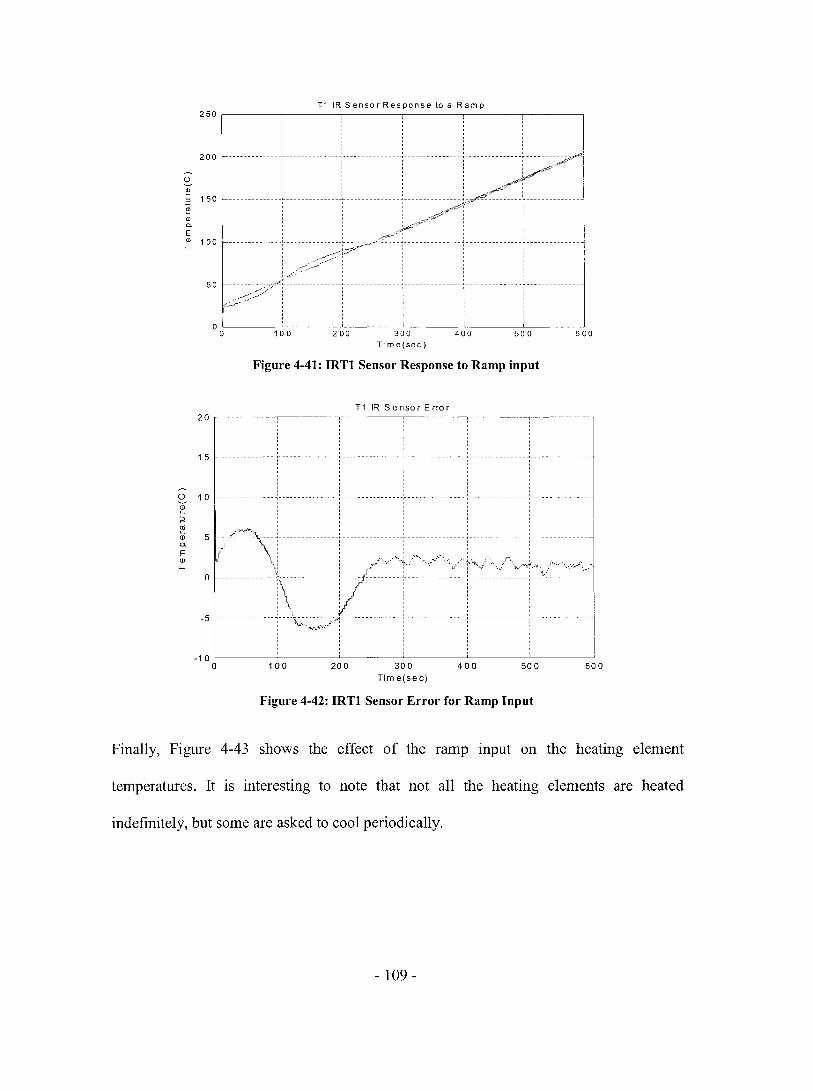
T11RSensorResponsetoa Ramp 250 ,-------~------~------~------~------~------_,
1 l , 1
l ':: ~ ••••••• • ••••• I •••••••••••••• [=~"1~~/E=Ji:~=/· : /~ : : : 1 p;::::;/" i i i
50/::~;:;;"";T--------------:---------------(-------------(-----------
~- :: ;
; ; ; ,
°0-L-----~1LOO~----~2~OO~----~3~0~0------4~OLO------5~OLO~----~600
20
15
Ü 10
~ .2 ~ Q) 5 "-E Q)
f-0
-5
Tim e(sec)
Figure 4-41: IRT1 Sensor Response to Ramp input
100 200
T1 IR Se nso r E rrO r
300 Time(sec)
400 500
Figure 4-42: IRT1 Sensor Error for Ramp Input
600
FinaIly, Figure 4-43 shows the effect of the rarnp input on the heating elernent
ternperatures. It is interesting to note that not aIl the heating elernents are heated
indefinitely, but sorne are asked to cool periodicaIly.
- 109 -

Heating element response to Ramp input 350~----~------~----~------~----~----~
300
250 f----------
100
50
O~----~------~----~------~----~----~
o 100 200 300 Time(sec)
400 500
Figure 4-43: Heating Element Response to Ramp Input
600
Through aIl this discussion, the objective of controlling the temperature at different
locations on the surface of a plastic sheet in real-time has been achieved. The IR sensor
sheet temperature measurements can be controlled to within IOC of a final steady-state
value, or within 2°C of a ramp value. The ramp input is more typical of the
thermoforming process, as each sheet will only be in the oven for a short length of time,
and will not typically attain a steady-state value. With more precise desired input
functions, the simple linear control methods devised in this chapter could be proven to be
very useful in eliminating rejected parts, as weIl as decreasing the heating time. Both of
these would increase throughput on a typical forming machine, a major benefit to
industry.
- 110-

Chapter 5 Conclusion
5.1 Summary
The objective of this thesis is twofold: to develop a reliable state-space model of sheet
reheat for simulation analysis, and to develop and test an in-cycle real-time temperature
controller for the sheet reheat stage of the thermoforming process. The primary reasons
for this are to decrease the formed part rejection rate, and optimize the heating time.
These will then lead to increased machine throughput, and even potentially decrease
machine-related energy costs. A brief review of the literature foIlowed, investigating the
prospects of other real-time control algorithms implemented in industrial settings as weIl
as the advantages and disadvantages ofworking with infrared technology.
In the next chapter, a model ofthe sheet heating phase was developed. Basic heat transfer
theory was explained and then applied to the thermoforming sheet-heater system. The
existing discretized sheet model was then improved by using the Beer-Lambert law to
explain energy absorption within the sheet. The new state-space model was tuned to
experimental results with great success, as most tuned model parameters were within
their nominal range.
Finally, the real-time aspect was investigated. The dimensions of the existing oyen were
given, as well as the characteristics of both the actuators and the sensors. Infrared
thermometry was briefly explained. The existing control structure was examined, and the
real-time operating software was also described.
The real-time control algorithm was proposed in the final section. A linearization of the
- 111 -

non-linear state-space system was perfonned about a typical operating point. Inner-Ioop
heating element controllers were designed and tested. The steady-state gain matrix
between heating elements and sheet surface temperatures was detennined next, enabling
the modeling of the sheet surface temperature transfer functions. From these transfer
functions, outer-Ioop PI controllers were designed. Finally, these were tested in real-time
using both steady-state inputs and ramp inputs (to simulate a typical thennofonning mn).
The ramp results were satisfactory, maintaining the sheet surface temperatures within 5°C
of the increasing ramp value.
To the author's knowledge, this was the first successful implementation of a real-time
sheet temperature controller for thennofonning.
5.2 Recommendations and Future Work
The development of the real-time sheet reheat controller in thennofonning is far from
complete. The work demonstrated in this thesis is but a small fraction of what remains to
be done, before a commercially viable sheet reheat controller can be finalized.
The remaining IR sensors must first be installed into the oven, and the new gain matrix
for all sensors must be calculated, using the D-M-E insulator sheet. This will give a more
complete sheet surface temperature distribution, for both the top and bottom of the sheet.
The sheet temperature transfer functions must then be identified for each IR sensor
location, after which new PI controllers can be tuned and implemented. These new
controllers will then be tested in real-time using the RT-LAB modeling software, both for
step and ramp inputs. The ramp testing will then be repeated using HDPE sheets of
different thicknesses, to demonstrate the effectiveness of the controllers in maintaining a
- 112 -

desired surface temperature distribution.
However, this only solves half the sheet reheat problem posed in the thesis introduction.
The sheet heating time is not optimized in any way using these real-time PI controllers.
But a tool has been developed to determine the sheet centerline temperature, namely the
discretized sheet mode!. It has been established that there is no way to produce a
formable part while measuring internaI sheet temperatures using contact thermocouples.
These would cause damage to the sheet, and most likely cause a rejected part. The
discretized sheet model could then be used in real-time, in conjunction with the IR
surface temperature measurements, in order to calculate the temperature at any depth
within the sheet. Similar to the way Kalman filters are used for estimating position in
aircraft control, the sheet model can be used to estimate the internaI temperatures of the
sheet. The IR sensor measurements are then used as time-varying boundary conditions,
and as inputs to the Kalman filter. In this way, controllers can then be designed to
optimize the heating time, by finding the correct parameters to increase the temperature at
the sheet centre to the minimum forming temperature.
To fully demonstrate the effectiveness of this type of real-time model-based control
system, the system would have to be tested against the existing open-Ioop "tweaking"
type control on an industrial scale. A typical batch should first be run for a given part
under normal open-loop conditions, and repeated using the new model-based real-time
in-cycle controller. The controller should decrease the part rejection rate, even while
decreasing the heating time per part.
- 113 -

Chapter 6 References
[1] Throne, James L. Radiant Heat Transfer in Thermoforming, ANTEC conference
1995, pp.810-821.
[2] Lappin, J.F, Martin, P.J., Sheet Temperature Measurement in Thermoforming,
ANTEC conference 1996, pp.878-882.
[3] Yousefi, A., Bendada, A., DiRaddo, R., Improved Modeling for the Reheat Phase in
Thermoforming Through an Uncertainty Treatment of the Key Parameters, Polymer
Engineering and Science, May 2002, Vol. 42, No. 5, pp.1115-1129.
[4] Duarte, F.M., Covas, J.A., IR Sheet Heating in roll-Jed Thermoforming Part 1 -
Solving direct and inverse heating problems, Plastics, Rubber and Composites 2002, Vol.
37, No. 7, pp.307-317.
[5] Duarte, F.M., Covas, J.A, IR Sheet Heating in roll-Jed Thermoforming Part II -
Factors Influencing Reverse Heating Solution, Plastics, Rubber and Composites 1 Jan
2003, Vol. 32, No. 1, pp.32-39.
[6] Monteix, S. et al., Experimental study and numerical simulation of prefonn or sheet
exposed to infrared radiative heating, Journal of Materials Processing Technology 119
(2001), pp.90-97.
[7] Bugbee, B., Droter, M., Monje, O., Tanner, B., Evaluation and Modification of
commerical infrared transducers for leaf temperature measurement, Advanced Space
Research, Vol. 22, No. 10, pp.1425-1434, 1998.
[8] Schmidt, F.M., Le Maoult, Y., Monteix, S., Modelling of infrated heating pro cess of
thermoplastic sheet used in thermoforming process, Journal of Materials Processing
- 114-
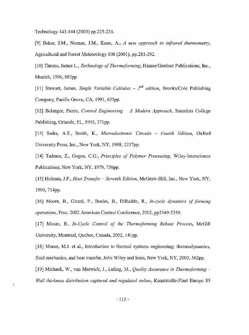
Technology 143-144 (2003) pp.225-231.
[9] Baker, J.M., Noman, J.M., Kano, A., A new approach to infrared thermometry,
AgricuItural and Forest Meteorology 108 (2001), pp.281-292.
[10] Throne, James L., Technology ofThermoforming, Hanser/Gardner Publications, Ine.,
Munich, 1996, 882pp.
[11] Stewart, James, Single Variable Calculus - 2nd edition, Brooks/Cole Publishing
Company, Pacific Grove, CA, 1991, 635pp.
[12] Belanger, Pierre, Control Engineering - A Modern Approach, Saunders College
Publishing, Orlando, FL, 1995, 271pp.
[13] Sedra, A.S., Smith, K., Microelectronic Circuits - Fourth Edition, Oxford
University Press, Inc., New York, NY, 1998, 1237pp.
[14] Tadmor, Z., Gogos, c.G., Principles of Polymer Processing, Wiley-Interscience
Publications, New York, NY, 1979, 736pp.
[15] Holman, J.P., Heat Transfer - Seventh Edition, McGraw-Hill, Ine., New York, NY,
1990, 714pp.
[16] Moore, B., Girard, P., Boulet, B., DiRaddo, R., In-cycle dynamics of forming
operations, Proc. 2002 American Control Conference, 2002, pp3349-3350.
[17] Moore, B., In-Cycle Control of the Thermoforming Reheat Process, McGill
University, Montreal, Quebee, Canada, 2002, 141pp.
[18] Moran, M.J. et al., Introduction to thermal systems engineering: thermodynamies,
fluid mechanics, and heat transfer, John Wiley and Sons, New York, NY, 2003, 562pp.
[19] Michaeli, W., van Marwick, J., Luling, M., Quality Assurance in Thermoforming
Wall thickness distribution captured and regulated online, Kunststoffe-Plast Europe 85
- 115 -

(9), pp.1316-1320.
[20] Sala, G., Di Landro, L., Cassago, D., A numerical and experimental approach to
optimize sheet stamping technologies: polymers thermoforming, Materials and Design 23
(2002), pp.21-39.
[21] Safarty, M. et al., Advance Pro cess Control Solutions for Semiconductor
Manufacturing, IEEE/SEMI Advanced Semiconductor Manufacturing Conference, 2002,
pp.l 02-1 06.
[22] Petterson, M., Stenstrom, S., Modelling of an electric IR heater at transient and
steady state conditions - Part II: modelling a paper dryer, International Journal of Heat
and Mass Transfer 43 (2000), pp.1223-1232.
[23] DiRaddo, R., Girard, P., Chang, S., Process drift and model-based control of
forming operations, Proc. 2002 American Control Conference, 2002, pp.3588-3593
[24] Hossain, A., Choudhury, Z.A., Suyut, S., Statistical Pro cess Control of an Industrial
Pro cess in Real Time, IEEE Transactions on Industry Applications, Vol. 32, No.2, 1996,
pp.243-249.
[25] Peng, J, et al., Real Time Optimization of Robotic Arc Welding Based on Machine
Vision and Neural Networks, Proceedings of the 24th Annual Conference of the IEEE,
vol.3, 1998, pp.1279-1283.
[26] Boulet, B. et al., Control of the Thermoforming Process, 16èmes Entretiens Jacques
Cartier Colloquium on Polymer Reaction Engineering: Modelling, Optimisation and
Control, Dec 2-4, 2003.
[27] Thermalert® MID™ MIC™ Miniature IR Sensor Operator 's Guide, Raytek
Corporation, Rev.C, 01102, http://www.raytek-
- 116-

northarnerica.com/adrnin!file handler12ae6092f570efabge577 de9b6820919cll 051816133
/MID eng RevC Print.pdf
[28] Visionary Solution™ Ca ta log: Section 7 Radiant Pro cess Heaters, TEMPCO
Electric Heater Corporation, 2002, 46pp., http://www.ternpco.com/Catalog/Section%207-
pdf/Section%2007.pdf
[29] Gruner, K-D., Principles oiNon-Contact Temperature Measurement, Raytek
Corporation, Rev. B, 2003, 32pp., http://www.raytek-
northarnerica.com/adrnin!file handler/2ae6092f570efabge577 de9b6820919c/1 017776674
/IR Theory RevB LR.pdf
[30] RT-LAB v6.2 User's Manual, Opal-RT Technologies, Inc., Rev. A, January 2003,
Il Opp., http://support.opal-rt.com/cornrnon! docs/pdf/rt-Iab usersrnanual. pdf
- 117 -

Appendix A: List of Polymers
Abbreviation
ABS
CPET
PET or APET
HOPE
LOPE
HIPS
PC
PMMA
PS or PA
PP
PS
PUR
PVC
Po/ymer Definition
Poly (acrylonitrile-butadiene-styrene)
Crystalline polyester (polyethylene terephthalate)
Amorphous Polyester (polyethylene terephthalate)
High-density polyethylene
Low-density polyethylene
High-impact polystyrene
Polycarbonate
Acrylic (polymethyl methacrylate)
Nylon
Polypropylene
Polystyrene
Polyurethane
Polyvinyl chloride
- 118 -

Appendix B: D-M-E Insulator Sheet Specifications
• ASBESTOS-FREE MATERIAL • HIGH COMPRESSION STRENGTH • MACHINABLE WITH HIGH SPEEO
CUTTING TOOLS
GENERAL DATA
ModuIus cl Elœti<ily in Comp'eusiion
Tnermal Concb.lcttvtl:y
f~~~~tnl ~F)
,AS1M D,:22'?)
("STill D-229)
(ASTMCl77)
49.400 psi '" '15F 27,200 psi '" 3OO'F 'U3!})OO ""î Af; J,OO'F 17.100 p-$i at:SOO'F 15,000 ps. '" 55O'F tAt • 10' psi al 75'" ;U);I[ 10"psi.:.t42S'F
1.9 et 75 F ::1,1 at425'F
D-M-E Standard
High Temperature Insulator Sh •• ts
FOR PLASTICS MOLeS AND DIE CAST DIES Q-M-E High Temperature Insulator Sheets are USEi>d on motds and dies between the top clamping plate and the stationary platen. and between the boUom of the ejectar housing and the movabla platen. The thermal insuJating properties of this unique asbestos- free. glass-relnforced pOlymer composite Înhibit heal transfer from Ihe mold to the platen. or trom the platen to the mold (dependîl19 on the al;>pli(,.l"Ilion). whioh helps conserve energy and pralong machine hte. Ttlese sheets have excellent non-deformation characteristlcs and a compressive strength- which is higher than asbestos and mica materlals. Compression molded for high Impact strength. IhAy arA Supplie<l mlcro-flnlshed top and botte,". parallel wilhin '" .002.
ENERGY SAVIN OS
'l, THICt<-Zl.M18BTU/br '1. THICK = 31.1104 BTUlhr
HIGH TEMPERATURE INSULATOR SHEETS
Special sizes .available on special oroer: Mat<. Jength %II: 96d Max, thickn9SS - 1 ft Max. width 48~ Min. Ihlckness ~ "l'.
- 119 -
aTlS-1 2 ItTIS·2436,2
HTI&36311-4
Installation; U .... v. ·20 fiat h .... d ~ Drill &. Tap base ta suit

Appendix C: Non-Linear Model MATLAB code
% function Thermal light() % % (c) Guy Gauthier ing. and Mark Ajersch % % 12 juillet 2004 % % This function determines the state-space model of the plastic sheet temperatures. % It also compares the model output to an input test vector, for tuning purposes. % % Inputs: - Experimental test name % - Bottom Heat flag, Top heat flag % - Input Heater Settings % % Outputs: - Nodal sheet temperature distributions % - Error fcn between model and test
test name = input('\nPlease enter Test Name here: '); H_bottom = input('Heating from bottom (1 for Yes, 0 for No) '); H_top = input('Heating from top (1 for Yes, 0 for No): '); Heater_temp = input('Enter heater setpt temperatures (in C) ');
h 0.5; %delta time N 10000; %number of points t (O:h:N*h); %time vector
Zt = 0.141; %distance in m from sheet to upper aven Zb = 0.171; %distance in m from sheet to lower aven Vft AAA_view_factors-patrick(Zt); %view Factor top Vfb AAA_view_factors_patrick(Zb); %view Factor bottom
sbc 5.66ge-8; %boltzmann constant emis = 0.45; %effective emissivity
l = 0.012/4; % delta thickness Tambt = 115+273; %ambient air temperature top Tambb = 145+273; %ambient air temperature bottom hh 30; % Convection coefficient kk = (0.128/1)*.9; % Conduction coefficient
rho = 850; %density Cp 1700; %heat capacity
sx 76.67e-3; %sheet zone width sy 102.5e-3; %sheet zone height 10 304.8e-3; %oven zone size
sevt = sbc*emis*Vft*(10A 2 / sx*sy); %finding upper and lower multiplying factors sevb = sbc*emis*Vfb*(10A 2/ sx*sy);
- 120-

%ct = l/(rho*Cp*I);
x(:,l) (22+273)*ones(S*6,1); %initial sheet temps
%H_top 1; % If 0, heaters off # If l, heaters work %H bottom 0;
B coef 30; %absorption coefficient Beer 1 exp(-B_coef*I/2); %Beer-Lambert output for external layer Beer 2 exp (-B_coef*l) ; %Beer-Lambert output for internaI layer
u ([ones(6,1)*(Heater_temp+273)*H_top;ones(6,1)*(Heater_temp+273)*H_botto
ml) .A4; %input vector
BBI []; BB2 []; SEVt [0; 0 ; 0; 0 ; 0 ; 0] ; 8EVb [0;0;0;0;0;0] ; RADl=[]; RADS=[]; %initializations for k=1:6;
SEVt = 8EVt + sevt(:,k); SEVb = SEVb + sevb ( : , k) ; BBI = [BBl;2*sevt(k, :)*(l-Beer_l);
sevt(k, :) *Beer_l* (1-Beer_2) ; ... sevt(k, :)*Beer l*Beer 2*(1-Beer 2) ; .. . sevt(k, :)*Beer=1*Beer=2 A2*(1-Be;r_2); .. . 2*sevt(k, :)*Beer_l*Beer_2 A3*(1-Beer_l)]; %coefficients
for transmitted energy top BB2 = [BB2;2*sevb(k, :)*Beer l*Beer 2 A3*(1-Beer 1); .. .
sevb(k, :)*Beer_l~Beer_2A2*(1-Beer_2); .. . sevb(k, :) *Beer_l*Beer_2* (1-Beer_2) ; .. . sevb(k, :)*Beer_l*(1-Beer_2); 2*sevb(k, :)*(l-Beer_l)]; %coefficients for transmitted
energy bot tom RADI = [RADI i2*(1-Beer_l); ...
Beer_l*(1-Beer_2); ... Beer l*Beer 2*(1-Beer 2); .. . Beer-l*Beer-2 A2*(1-Be;r 2) i .. .
absorbed RADS
2*Be;r_l*Be;r_2 A3*(1-Be;r_l)] ; energy top = [RADS ;2*Beer l*Beer 2 A3*(1-Beer 1); .. .
bot tom end BB = [BBI BB2];
for k = l:N
Beer_l~Beer_2A2*(1-Beer_2); .. . Beer_l*Beer_2*(1-Beer_2); .. . Beer_l*(I-Beer_2); ... 2*(1-Beer_l)]; %coefficients
if mod(k,lOO)==O fprintf('*'); end if mod (k, 1000) ==0 fprintf (' l '); end if mod(k,4000)==0 fprintf('\n'); end %rho = diag(I./(lOOO*Rho-poly_HDPE(x(:,k)))); %Cp = diag(l./Cv-poly_HDPE(x(:,k))); ct = l/(l*Cp*rho); B = ct*h*BB; 8Sl = []; S8S= [];
- 121 -
%coefficients for
for absorbed energy

for kl = 1:6 for k2 = 1:5
SSl [SSl SEVt (kl) *x (1+ (kl-l) *5, k) A 4 *H_top] ; top surface
%radiant energy striking
SS5 [SS5 SEVb (kl) *x (kl*5, k) A 4 *H_bottom]; %radiant energy striking bottom surface
end end Sh = ct*h* (diag(SSl) *RAD1+diag(SS5) *RAD5) ; %radiant energy absorbed
by sheet Qrad B*[u(1:6)*H_top;u(7:l2)*H_bottom] - Shi %net radiant energy
dx ct*h*deltaTemp_six_zones(x(:,k),Tambt,Tambb,hh,kk); %conduction and convection energies
x(:,k+l) = x(:,k) + dx + Qrad; %total energy distribution end
% Plotting Simulated vs. Experimental results
data = load(test _name) ; time = data (: , 1) ; Tl data (:,2) ; %exp temperature T3 = data ( : ,4) ; %exp temperature T9 = data(:,8); %exp tempe rature Tll = data(:,lO); %exp temperature
% plotting experimental curves figure (3)
at lmm at 3mm at 9mm at llmm
P3= plot (time, Tl, 'r',time, T3, 'g' ,time, T9, 'b',time, Tl1, 'k'); set(P3(1), 'LineWidth' ,2.5, 'LineStyle', '--'); set(P3(2), 'LineWidth',2.5, 'LineStyle',': '); set(P3(3), 'Linewidth',2.5, 'LineStyle', ,-. '); set(P3 (4), 'LineWidth' ,2.5); xlabel('Time (in sec) ') ylabel('Temperature (in C) ,) title('Experimental Temperature Curves at 420C for l2mm sheet') grid; legend ( 'lmm' , '3mm' , , 9mm' , , llmm' ,0)
total = max (time) ; if total > N
fprintf('Simulation shorter than file length, please increase to at least %f seconds', max(time)); else
end
%concatenate simulation to data file length index max(time)-mod(max(time) ,1); x7 sh x(7,1:index*2)-273; x9 sh x(9,1:index*2)-273; T3 sh T3(2:length(T3)-1); T9 sh T9(2:length(T9)-1);
%calculating errors error T3 T3 sh - x9 sh'; error T9 T9 sh - x7 ShI;
- 122 -

% plotting errors at 3mm and 9mm depths figure (4) P4 =plot(time(2:length(time)-1), error_T3, lb' ,time(2:length(time)-1), error_T9, 'r'); grid; set(P4(1), 'LineStyle', ,--, o 0]);
'Color', [0 1 1]); set (P4 (2), 'Color', [0
xlabel ( 'Time (sec)' ); ylabel ( 'Temperature (OC)' ) ; title ( 'Simulation Error (vs. Experimental Data) at 280C for 12mm Sheet'); legend('Error at 3mm', 'Error at 9mm',O)
% calculating steady-state errors ss_error3 error_T3(length(error_T3»/max(T3_sh)*100; ss_error9 = error_T9(length(error_T9»/max(T9 sh)*100;
fprintf ( , \nThe percent error at steady-state ss error3); -fprintf ( 'The percent error at steady-state ss error9) ;
% plotting centre zone temperatures
figure (2) P2=plot(t(1:index*2) ,x(6:10,l:index*2)-273); grid
for 3mm
for 9mm
is %5.2f%% \n' ,
is %5.2f%% \n' ,
set(P2(1),'LineWidth',2.5, 'LineStyle',':', 'Color', [0 0 0]); set(P2(2), 'LineWidth',2.5, 'LineStyle', ,-. '); set(P2(3), 'Linewidth',2.5, 'LineStyle', '--Il; set(P2(4), 'LineWidth' ,2.5, 'LineStyle', '-. '); set (P2 (5) , 'LineWidth' ,2.5) ; xlabel('Time (sec) '); ylabel('Temperature (OC) '); title('Simulated Model Temperature Curves at 280C for 12mm Sheet'); legend('Top Surface', '9mm', '6mm', '3mm', 'Bottom Surface',O)
function dx deltaTemp_six_zones(x,Tambt,Tambb,h,k)
% deltaTemp_6_zones at any no de % %
calculates the incremental change in temperature
due to conduction and convection only
% Synopsys: dx %
deltaTemp_six_zones(x,SEV,Tamb,h,k)
% Entrées: x % Tambt % Tambb % h % k nodes) % % Sorties: dx %
actual temperatures (in oK) top air temperature (in oK) top air temperature (in oK) convection coefficient = conduction coefficient (divided by distance b/w 2
Temperaure increments (in OK)
% (c) Guy Gauthier ing. and Mark Ajersch % % 12 juillet 2004
- 123 -

dx = [2*(h*(Tambt-x(1» + k*(x(2)-x(1»)i ... k*(x(l) -2*x(2)+x(3» i k* (x(2) -2*x(3)+x(4» i k* (x(3)-
2*x(4) +x(5» i ...
2* (h* (Tambb-x(5» + k* (x(4) -x(5») i .. .
2* (h* (Tambt-x(6» + k* (x(7) -x(6») i .. .
k* (x(6) -2*x(7)+x(8» i k* (x(7) -2*x(8) +x(9» i k*(x(8)-
2*x(9)+x(10»; ... 2*(h*(Tambb-x(10» + k*(x(9)-x(10»)i .. . 2*(h*(Tambt-x(11» + k*(x(12)-x(11»); .. . k* (x(l1) -2*x(12) +x(13» i k* (x(12) -2*x(13) +x(14»; k* (x (13) -
2*x (14l+x (15» ; ... 2* (h* (Tambb-x(15» + k* (x(14) -x(15»); .. . 2* (h* (Tambt-x(16» + k* (x(17) -x(16»); .. . k* (x (16) -2*x (17) +x (18» ; k* (x (17) -2*x (18) +x (19) ) i k*(x(18)-
2*x(19l+x(20» i ..•
2* (h* (Tambb-x(20» + k* (x(19) -x(20»); ... 2* (h* (Tambt-x (21» + k* (x (22) -x (21») i . .•
k*(x(21)-2*x(22)+x(23»i k*(x(22)-2*x(23)+x(24»i k*(x(23)-
2*x(24)+x(25» i ...
2* (h* (Tambb-x(25» + k* (x(24) -x(25»); .. . 2* (h* (Tambt-x(26» + k* (x(27) -x(26») i .. .
k* (x (26) -2*x (27) +x (28» ; k* (x (27) -2*x (28) +x (29» ; k*(x(28)-
2*x(29) +x(30»; ... 2* (h* (Tambb-x(30» + k* (x(29) -x(30»)] i
- 124-